tdot design division drainage manual - tn.gov · pdf filetdot design division drainage manual...
TRANSCRIPT

TDOT DESIGN DIVISION
DRAINAGE MANUAL
CHAPTER IV HYDROLOGY
TDOT DESIGN DIVISION DRAINAGE MANUAL January 1, 2010
i
TDO
T - RO
AD
WA
Y DESIG
N G
UID
ELINES
English
Revised:
01/01/99
CHAPTER 4 – HYDROLOGY
SECTION 4.01 – INTRODUCTION
4.01 INTRODUCTION ...........................................................................................4-1
SECTION 4.02 – DOCUMENTATION PROCEDURES
4.02 DOCUMENTATION PROCEDURES .............................................................4-2
SECTION 4.03 – DESIGN CRITERIA
4.03 DESIGN CRITERIA........................................................................................4-3
SECTION 4.04 – APPLICABLE METHODS
4.04 APPLICABLE METHODS ..............................................................................4-5 4.04.1 RATIONAL METHOD .....................................................................................4-7 4.04.1.1 Runoff Coefficient ........................................................................................4-7 4.04.1.2 Intensity ......................................................................................................4-8 4.04.1.3 Time of Concentration .................................................................................4-9 4.04.1.3.1 Travel Time - Overland Flow .......................................................................4-9 4.04.1.3.1.1 Travel Time - Sheet Flow .......................................................................... 4-10 4.04.1.3.1.2 Travel Time - Shallow Concentrated Flow ................................................. 4-12 4.04.1.3.2 Travel Time - Pipe, Gutter, and Channel Flow ........................................... 4-13 4.04.1.4 Drainage Area ........................................................................................... 4-14 4.04.1.5 Procedures ................................................................................................ 4-15 4.04.2 USGS REGRESSION EQUATIONS FOR RURAL AREAS .......................... 4-15 4.04.2.1 Background ............................................................................................... 4-15 4.04.2.2 Procedures ................................................................................................ 4-20 4.04.2.2.1 Single Variable Regression Equations ...................................................... 4-20 4.04.2.2.2 Flood Frequency Computer Application .................................................... 4-20 4.04.3 USGS REGRESSION EQUATIONS FOR URBAN AREAS .......................... 4-21 4.04.3.1 Background ............................................................................................... 4-21 4.04.3.2 Procedures ................................................................................................ 4-22 4.04.4 USGS REGRESSION EQUATIONS FOR THE CITY OF MEMPHIS AND SHELBY COUNTY URBAN AREAS ................................................... 4-22 4.04.4.1 Background ............................................................................................... 4-22 4.04.5 OTHER HYDROLOGIC METHODS ............................................................. 4-23 4.04.5.1 Introduction ............................................................................................... 4-23 4.04.5.2 Sources of Existing Flow Data ................................................................... 4-23 4.04.5.3 Hydrologic Models Involving Detention (HEC-1, HEC-HMS, AND TR-55) ....................................................................................................... 4-23 4.04.5.3.1 Hydrologic Model Loss Rate and Unit Hydrograph Methodology .......................................................................... 4-23
TDOT DESIGN DIVISION DRAINAGE MANUAL January 1, 2010
ii
TDO
T - RO
AD
WA
Y DESIG
N G
UID
ELINES
English
Revised:
01/01/99
4.04.5.3.2 Rainfall Distributions ................................................................................. 4-25
SECTION 4.05 – ACCEPTABLE SOFTWARE
4.05 ACCEPTABLE SOFTWARE ........................................................................ 4-27
SECTION 4.06 – APPENDIX
4.06 APPENDIX .................................................................................................. 4A-1 4.06.1 FIGURES AND TABLES ............................................................................. 4A-1 4.06.2 EXAMPLE PROBLEMS ............................................................................ 4A-35 4.06.2.1 Rational Method Example Problems ...................................................... 4A-35 4.06.2.1.1 Simple Drainage Area Design Discharge Example ................................. 4A-35 4.06.2.1.2 Complex Drainage Area Design Discharge Example ............................. 4A-41 4.06.2.1.3 Computer Application ............................................................................. 4A-47 4.06.2.2 Regression Equation Examples ............................................................. 4A-48 4.06.2.2.1 Rural Regression Example ..................................................................... 4A-48 4.06.2.2.2 Statewide Urban Regression Example ................................................... 4A-52 4.06.3 GLOSSARY .............................................................................................. 4A-56 4.06.4 REFERENCES ......................................................................................... 4A-59 4.06.5 ABBREVIATIONS ..................................................................................... 4A-61

TDOT DESIGN DIVISION DRAINAGE MANUAL January 1, 2010
4-1
TDO
T - RO
AD
WA
Y DESIG
N G
UID
ELINES
English
Revised: 01/01/99
SECTION 4.01 - INTRODUCTION
This chapter presents the Tennessee Department of Transportation (TDOT) procedures and accepted methodologies for hydrologic analyses for roadway design. The procedures and methodologies presented in this chapter assume that the designer has a basic understanding of the science of hydrology and its principles. Additionally, the designer should also be familiar with regulations and requirements of various State and Federal agencies that regulate water-related construction as they may affect TDOT projects.
Hydrology is generally defined as the science dealing with the interrelationship between
water on and under the earth and in the atmosphere. For this manual, hydrology will consist of estimating storm water runoff discharge rates and/or volumes from precipitation for the design of the highway drainage system and any required cross drainage structures. In general, only computed peak flow rates will be required from the hydrologic analyses. Runoff hydrographs and volumes will be required only under special circumstances such as when designing a permanent detention basin or temporary sediment basin.
In urban or urbanizing areas, the designer should consider the impact changing land use
conditions would have on the size and capacity of the roadway drainage system and cross drainage structures.
The sections of this chapter of the Manual will present the hydrologic design criteria for
the components of the roadway drainage system and cross drainage structures, recommended methods, and approved software. The Appendix of this chapter contains example computations and procedures of the various topics presented within this chapter. Additionally the Appendix contains a glossary or terms, list of references, and a list of abbreviations used in the text of this chapter. All of these are included to assist the designer during the design process.
TDOT DESIGN DIVISION DRAINAGE MANUAL January 1, 2010
4-2
TDO
T - RO
AD
WA
Y DESIG
N G
UID
ELINES
English
Revised: 01/01/99
SECTION 4.02 - DOCUMENTATION PROCEDURES
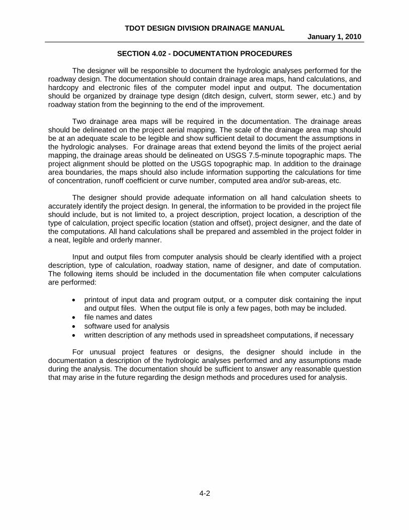
The designer will be responsible to document the hydrologic analyses performed for the roadway design. The documentation should contain drainage area maps, hand calculations, and hardcopy and electronic files of the computer model input and output. The documentation should be organized by drainage type design (ditch design, culvert, storm sewer, etc.) and by roadway station from the beginning to the end of the improvement.
Two drainage area maps will be required in the documentation. The drainage areas
should be delineated on the project aerial mapping. The scale of the drainage area map should be at an adequate scale to be legible and show sufficient detail to document the assumptions in the hydrologic analyses. For drainage areas that extend beyond the limits of the project aerial mapping, the drainage areas should be delineated on USGS 7.5-minute topographic maps. The project alignment should be plotted on the USGS topographic map. In addition to the drainage area boundaries, the maps should also include information supporting the calculations for time of concentration, runoff coefficient or curve number, computed area and/or sub-areas, etc.
The designer should provide adequate information on all hand calculation sheets to
accurately identify the project design. In general, the information to be provided in the project file should include, but is not limited to, a project description, project location, a description of the type of calculation, project specific location (station and offset), project designer, and the date of the computations. All hand calculations shall be prepared and assembled in the project folder in a neat, legible and orderly manner.
Input and output files from computer analysis should be clearly identified with a project
description, type of calculation, roadway station, name of designer, and date of computation. The following items should be included in the documentation file when computer calculations are performed:
• printout of input data and program output, or a computer disk containing the input
and output files. When the output file is only a few pages, both may be included. • file names and dates • software used for analysis • written description of any methods used in spreadsheet computations, if necessary
For unusual project features or designs, the designer should include in the
documentation a description of the hydrologic analyses performed and any assumptions made during the analysis. The documentation should be sufficient to answer any reasonable question that may arise in the future regarding the design methods and procedures used for analysis.

TDOT DESIGN DIVISION DRAINAGE MANUAL January 1, 2010
4-3
TDO
T - RO
AD
WA
Y DESIG
N G
UID
ELINES
English
Revised: 01/01/99
SECTION 4.03 - DESIGN CRITERIA
Design frequency for roadway drainage facilities is based on achieving a balance between construction cost, maintenance needs, amount of traffic, potential flood hazard to adjacent property, and expected level of service. The design frequencies presented in Table 4-1 are the minimum that will achieve this balance for the various road classifications and types of drainage facility.
Cross structures should be designed based on the design frequencies in Table 4-1 such
that they:
1. Shall not significantly increase the flood hazard for adjacent property and 2. Shall permit maintenance of traffic on roads and streets under design flood conditions.
Storm drainage structures should be designed based on the design frequencies in Table
4-1 such that they:
a. Shall not significantly increase the flood hazard for adjacent property and b. Shall limit the encroachment onto the traveled lanes which could cause a hazard to
traffic.
The design frequency for a given flood is the reciprocal of the probability that a flood will be equaled or exceeded in a given year. If a flood event has a 10 percent chance of being equaled or exceeded in a year, the flood event will be equaled or exceeded on average every 10 years. The designer should note that the 10-year flood event will not be equaled or exceeded once every 10 years, but has a 10 percent chance of being equaled or exceeded in any given year. Therefore, the 10-year flood event could conceivably occur in consecutive years, or possibly even more frequently.

TDOT DESIGN DIVISION DRAINAGE MANUAL January 1, 2010
4-4
TDO
T - RO
AD
WA
Y DESIG
N G
UID
ELINES
English
Revised: 01/01/99
Interstate System and Arterial With Full Access
Control
Arterial Without Full
Access Control
Collector Local Road
Inlet Design Frequency 50-yr 10-yr 1 10-yr 1 10-yr
Sewer Design Frequency
50-yr 10-yr 1 10-yr 1 10-yr
Culvert Design Frequency
50-yr Check for
100-yr
50-yr Check for
100-yr
50-yr Check for
100-yr
50-yr Check for
100-yr
Roadway Freeboard 2 50-yr 50-yr 50-yr 50-yr
Ditch Design Frequency 50-yr 10-yr 1 10-yr 1 10-yr
1 50-year in Roadway Sag Sections 2 The design high water elevation should be at or below the bottom of the roadway subgrade.
Table 4-1
Hydrologic Design Criteria

TDOT DESIGN DIVISION DRAINAGE MANUAL January 1, 2010
4-5
TDO
T - RO
AD
WA
Y DESIG
N G
UID
ELINES
English
Revised: 01/01/99
SECTION 4.04 - APPLICABLE METHODS
This section of the chapter describes the hydrologic methods that are approved for use by the Tennessee Department of Transportation (TDOT). The designer should be familiar with the limitations of each of the methods so that appropriate methods are applied. There will be some projects where the approved methodologies are not applicable. The designer will need to be familiar with a variety of hydrologic methods to ensure the correct methodology is selected and used for these isolated circumstances. Any methodology not described in this section of the Manual must be approved by the TDOT Design Manager or the Hydraulics Section prior to any hydrologic analyses using the methodology.
Other hydrologic methods and software may be considered for use on TDOT projects at
the discretion of the Design Manager at the request of the designer. For other hydrologic methods and software to be considered, the designer will need to demonstrate that the method is appropriate for the intended application.
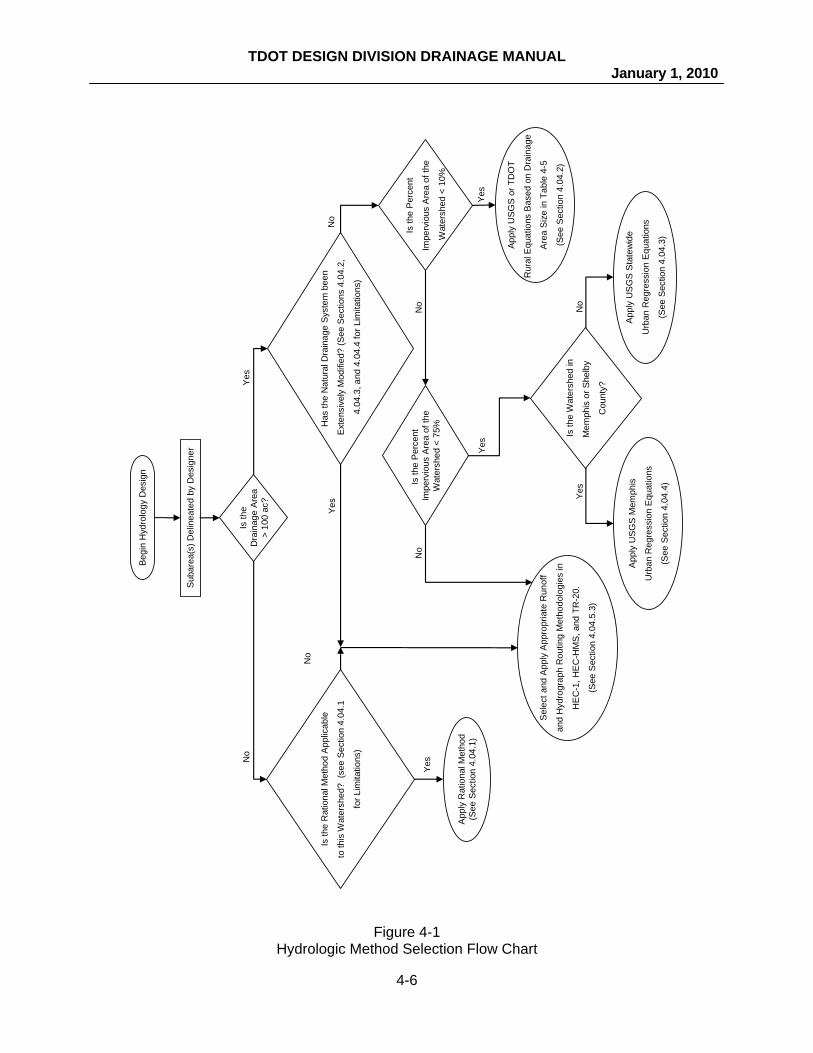
To assist the designer in selecting the appropriate hydrologic method, a flow chart is
shown in Figure 4-1. The first decision point is strictly based on drainage area. The rational method is the preferred method for all drainage areas less than 100 acres. The USGS regression equations for rural and urban areas are the preferred methods for drainage areas larger than 100 acres. These methods should be used for all projects unless they are not applicable due to the watershed conditions or the need for a runoff hydrograph.
The primary reason the preferred methods (Rational and USGS Regression Equations)
would not be applicable is due to man-made modifications in the watershed or to the stormwater conveyance system. A natural lake or man-made reservoir with sufficient storage volume to attenuate the peak flow rate for the design frequency is one example of when the preferred methods would not be applicable. The limitations of each method will be discussed in this chapter.
The software presented in the Appendix of Chapter 8 will be required for any TDOT
drainage design where the project will include a stormwater storage facility (existing or proposed). HEC-1 may be used if there is an existing HEC-1 model available.
If the design peak flow rate computed by the selected analysis method is greater than
500 ft3/s for the 50-year storm, the designer should indicate the location of the structure on the proposed roadway layout drawing. This drawing, along with the related drainage survey and hydrologic calculations, should be forwarded to the Hydraulic Design Section of the Structures Division. The Hydraulic Design Section will then furnish all of the necessary data to be shown on the plans for the particular structure. The designer will be responsible for incorporating this information into the design plans.
Table 4A-11 of the chapter Appendix may be used by the designer for quick reference
as to whether a watershed analysis should be forwarded to the Hydraulic Design Section or not. In general, if the watershed area being analyzed equals or exceeds the values contained in the table, then the 50-year storm discharge will be greater than 500 cubic feet per second; and the designer should forward the appropriate material to the Hydraulic Design Section.
TDOT DESIGN DIVISION DRAINAGE MANUAL January 1, 2010
4-6
Figure 4-1 Hydrologic Method Selection Flow Chart
Sel
ect a
nd A
pply
App
ropr
iate
Run
off
and
Hyd
rogr
aph
Rou
ting
Met
hodo
logi
es in
HE
C-1
, HE
C-H
MS
, and
TR
-20.
(See
Sec
tion
4.04
.5.3
)
App
ly R
atio
nal M
etho
d(S
ee S
ectio
n 4.
04.1
)
App
ly U
SGS
Mem
phis
Urb
an R
egre
ssio
n E
quat
ions
(See
Sec
tion
4.04
.4)
Appl
y U
SG
S S
tate
wid
e
Urb
an R
egre
ssio
n E
quat
ions
(See
Sec
tion
4.04
.3)
Appl
y U
SG
S o
r TD
OT
Rur
al E
quat
ions
Bas
ed o
n D
rain
age
Are
a S
ize
in T
able
4-5
(See
Sec
tion
4.04
.2)
Sub
area
(s) D
elin
eate
d by
Des
igne
r
Is th
e W
ater
shed
in
Mem
phis
or S
helb
y
Cou
nty?
Is th
eD
rain
age
Are
a>
100
ac?
Is th
e R
atio
nal M
etho
d A
pplic
able
to th
is W
ater
shed
? (s
ee S
ectio
n 4.
04.1
for L
imita
tions
)
Has
the
Nat
ural
Dra
inag
e S
yste
m b
een
Ext
ensi
vely
Mod
ified
? (S
ee S
ectio
ns 4
.04.
2,
4.04
.3, a
nd 4
.04.
4 fo
r Lim
itatio
ns)
No
Yes
No
Yes
Is th
e P
erce
nt
Impe
rvio
us A
rea
of th
e
Wat
ersh
ed <
10%
Yes
Is th
e P
erce
nt
Impe
rvio
us A
rea
of th
e W
ater
shed
< 7
5%
No
No
Yes
No
Yes
Begi
n H
ydro
logy
Des
ign
No
Yes

TDOT DESIGN DIVISION DRAINAGE MANUAL January 1, 2010
4-7
TDO
T - RO
AD
WA
Y DESIG
N G
UID
ELINES
English
Revised: 01/01/99
4.04.1 RATIONAL METHOD The Rational method is recommended for estimating the design storm runoff for drainage areas less than 100 acres. The Rational Method is the preferred method to be used when all of the required data is available. The Rational Method for computing peak storm runoff is expressed as Equation 4-1:
CiAQ = (4-1) Where: Q = peak rate of runoff, (ft3/s) C = weighted runoff coefficient representing a ratio of runoff to rainfall, (unitless)
i = average rainfall intensity for a duration equal to the time of concentration, for a selected return period, (in/hr)
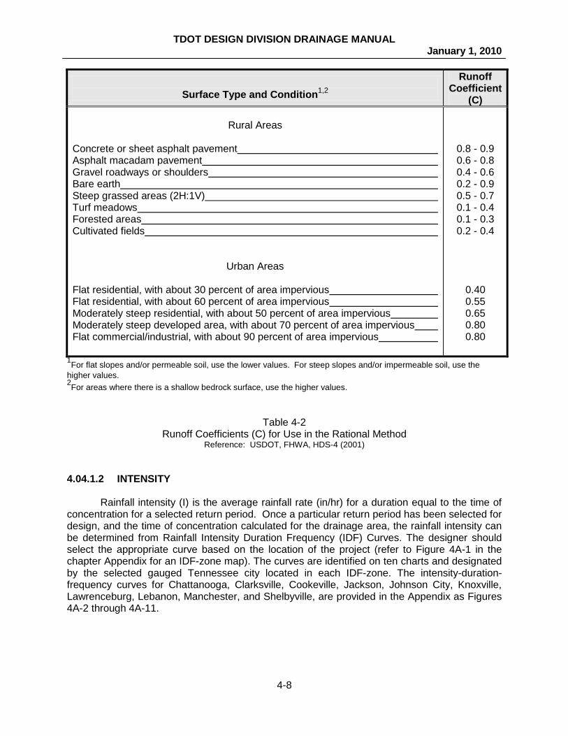
A = drainage area tributary to the point under design, (acres) Although the formula is not dimensionally correct (ft3/s vs. ac*in/hr), the conversion coefficient of 1.008 is ignored as being insignificant. For further technical information and details, refer to the 1965 and 2001 (metric) publications Hydraulic Design Series 4 (HDS-4) by the FHWA. The results obtained using the Rational Method to estimate peak discharge is very sensitive to the parameters selected for use in the equation. Under some conditions, peak runoff occurs before all of the drainage area contributes runoff to the point of analysis. The likelihood of error in the runoff estimate increases as the size and complexity of the drainage area increases. This likelihood of error is why the limit is set at 100 acres for applying the Rational Method by TDOT. The designer should use sound engineering judgment when estimating peak runoff values using the Rational Method. 4.04.1.1 RUNOFF COEFFICIENT The runoff coefficient represents the ratio of the rate of runoff to the rate of rainfall at an average intensity (i) when all the drainage area is contributing. The runoff coefficient is tabulated as a function of land use conditions; however, the coefficient is also a function of slope, rainfall intensity, infiltration, and other abstractions. The amount of water reaching the drainage structure is reduced by evaporation, transpiration, infiltration, and ponding. Two methods are commonly used for calculating the runoff coefficient. The first is to utilize known soil properties, infiltration rates, and land slopes. This method requires information from the Natural Resource Conservation Service (NRCS), formerly the Soil Conservation Service (SCS), and/or other agencies for pervious and impervious surface soil conditions. The second method for calculating the runoff coefficient is to utilize tables developed for various types of surface conditions and land use. Typical runoff coefficients to be used on TDOT projects are shown in Table 4-2.
Complex watersheds with several different types of land use will require that a weighted runoff coefficient be computed. The weighted runoff coefficient is computed by multiplying the runoff coefficient for each land use type by the respective area for each land use; summing these values, and then dividing the sum by the total area. An example of how to compute a weighted runoff coefficient is provided in the chapter Appendix. It should be noted that the Rational Method produces better results when the land use within the watershed being studied is fairly consistent over the entire area.
TDOT DESIGN DIVISION DRAINAGE MANUAL January 1, 2010
4-8
TDO
T - RO
AD
WA
Y DESIG
N G
UID
ELINES
English
Revised: 01/01/99
Surface Type and Condition1,2
Runoff Coefficient
(C)
Rural Areas Concrete or sheet asphalt pavement Asphalt macadam pavement Gravel roadways or shoulders Bare earth Steep grassed areas (2H:1V) Turf meadows Forested areas Cultivated fields
Urban Areas Flat residential, with about 30 percent of area impervious Flat residential, with about 60 percent of area impervious Moderately steep residential, with about 50 percent of area impervious Moderately steep developed area, with about 70 percent of area impervious Flat commercial/industrial, with about 90 percent of area impervious
0.8 - 0.9 0.6 - 0.8 0.4 - 0.6 0.2 - 0.9 0.5 - 0.7 0.1 - 0.4 0.1 - 0.3 0.2 - 0.4
0.40 0.55 0.65 0.80 0.80
1For flat slopes and/or permeable soil, use the lower values. For steep slopes and/or impermeable soil, use the higher values. 2For areas where there is a shallow bedrock surface, use the higher values.
Table 4-2 Runoff Coefficients (C) for Use in the Rational Method
Reference: USDOT, FHWA, HDS-4 (2001) 4.04.1.2 INTENSITY
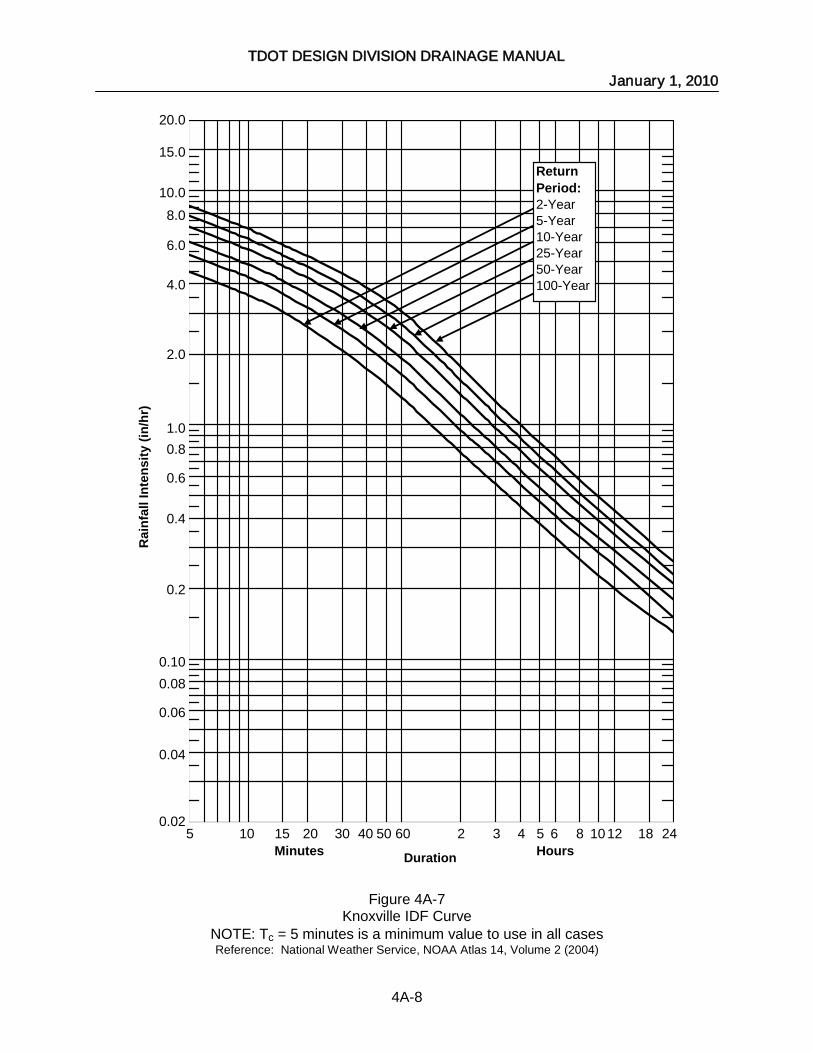
Rainfall intensity (I) is the average rainfall rate (in/hr) for a duration equal to the time of
concentration for a selected return period. Once a particular return period has been selected for design, and the time of concentration calculated for the drainage area, the rainfall intensity can be determined from Rainfall Intensity Duration Frequency (IDF) Curves. The designer should select the appropriate curve based on the location of the project (refer to Figure 4A-1 in the chapter Appendix for an IDF-zone map). The curves are identified on ten charts and designated by the selected gauged Tennessee city located in each IDF-zone. The intensity-duration-frequency curves for Chattanooga, Clarksville, Cookeville, Jackson, Johnson City, Knoxville, Lawrenceburg, Lebanon, Manchester, and Shelbyville, are provided in the Appendix as Figures 4A-2 through 4A-11.

TDOT DESIGN DIVISION DRAINAGE MANUAL January 1, 2010
4-9
TDO
T - RO
AD
WA
Y DESIG
N G
UID
ELINES
English
Revised: 01/01/99
4.04.1.3 TIME OF CONCENTRATION (TC)
Time of Concentration is the total time that it takes water to travel from the hydraulically most distant point in a watershed to the watershed’s outlet or the drainage structure being designed. The time of concentration may consist of overland flow (including sheet flow and shallow concentrated flow), pipe flow, channelized flow or a combination thereof. If there is a combination of flow types in the drainage basin, the time for each portion is identified as an individual travel time (tt). Equation 4-2 shows that summing the travel times for each reach will yield the time of concentration. As a general guideline, if the time of concentration is calculated to be less than 5 minutes, a minimum value of 5 minutes should be used.
tntttc ttttT ++++= 321 (4-2)
Several methods have been studied and proposed to compute the travel time for
overland flow. TDOT has selected several methods acceptable for their projects. The preferred method is the Kinematic Wave equation described in HDS-4. Another acceptable method for TDOT is the NRCS TR-55 methodology (Mannings' Kinematic Solution for overland flow travel time and NRCS Upland Method for shallow concentrated flow). A discussion of these methods is included in this section.
Methods for determining travel time for pipe flow, gutter flow, and channel flow have also been studied. The acceptable methods for TDOT projects include the Manning equation or a modified Manning equation for gutter flow. When the average water velocity is known, travel time can be calculated. Equation 4-3 is used to calculate travel time when an average water velocity is available:
V
Ltt ×=
60 (4-3)
Where: tt = travel time, (min)
L = length of flow, (ft) V = average velocity, (ft/s) (see Figure 4A-12) 60 = conversion factor from seconds to minutes
4.04.1.3.1 TRAVEL TIME – OVERLAND FLOW The overland flow time consists of the time required for runoff to flow over the ground surface to a channel, gutter, inlet, or pipe. The first portion of overland flow is termed sheet flow. After the water concentrates and collects in indentations on the ground such as swales, the flow becomes shallow concentrated flow. The sum of the two is overland flow. Some publications indicate that the Kinematic Wave Equation accounts for both the sheet flow travel time and the shallow concentrated flow travel time. TDOT follows the HDS-4 approach by limiting the equation's use to sheet flow. The components of overland flow are best shown by Equation 4-4 as: )flowedconcentratshallow(t)flowsheet(t)flowoverland(t ttt += (4-4)

TDOT DESIGN DIVISION DRAINAGE MANUAL January 1, 2010
4-10
TDO
T - RO
AD
WA
Y DESIG
N G
UID
ELINES
English
Revised: 01/01/99
4.04.1.3.1.1 TRAVEL TIME – SHEET FLOW
A portion of overland flow may be categorized as sheet flow. Friction in sheet flow is usually comprised of drag over the plane surface which may include obstacles such as litter, vegetation, sediment, and rocks. Sheet flow is normally considered when water flows at a depth of 0.1 feet (1.2 inches) or less. The time of concentration for sheet flow is approximated by utilizing the Kinematic Wave method or the NCRS Runoff method. It is not always apparent when flow changes from sheet flow to shallow concentrated flow. If shallow ridges, swales, or small channels are not evident in the field, it is reasonable to assume the runoff remains in sheet flow for a maximum of 300 feet. After 300 feet, it is assumed that storm runoff will typically find shallow ridges or swales on the ground's surface in which to collect. Once to this point, the water is termed shallow concentrated flow.
Kinematic Wave Theory for Computing Sheet Flow Travel Time
The Kinematic Wave Equation (Regan, 1971) for calculating sheet flow travel time was developed for flow on a plane surface of less than 300 feet in length, and is a derivative of Mannings Equation. Some publications have added assumptions to the equation and have permitted its use for shallow concentrated flow travel time and small channel or pipe travel time. TDOT chooses not to make these same assumptions and limits its use to sheet flow. For sheet flow, the Kinematic Wave method is the most physically correct approach according to HDS-4. The Kinematic Wave equation follows:
3040
6060
..
..
t SiLnCt = (4-5)
Where: tt = sheet flow travel time, (minutes)
C = 0.938 (constant) n = Manning roughness coefficient (see Table 4-3) L = sheet flow length, (ft) (Maximum is 300 feet) i = rainfall intensity, (in/hr) (see Figures 4A-2 through 4A-11) S = slope of the surface, (ft/ft) Solving the Kinematic Wave equation requires the designer to go through an iterative
process since both the travel time and rainfall intensity is unknown. Start by assuming a travel time, determine the rainfall intensity from the charts provided in the Appendix (see Figures 4A-2 through 4A-11), and then insert the rainfall intensity into the equation. When the assumed travel time approaches the travel time generated by the equation, the designer should use this value as the solution for the sheet flow travel time. If the equation is used for sheet flow estimation in a grassy area, the n value should be quite large (e.g., 0.45 for Bluegrass).
As per HDS-4 "This is necessary to account for the large relative roughness resulting
from water running through grass rather than over it as compared to channel flow conditions." A smaller n value should be used for smooth paved conditions (e.g., 0.011 for concrete). The Manning's n-values applicable for overland applications are included in Table 4-3. The designer should use an n-value based on the season of the year when the greatest likelihood of heavy rainfall will occur. This is especially pertinent to agricultural areas and roadside ditches. Farming practices alter the ground throughout the year and often different crops are planted over the years. The designer will need to make a judgment based on knowledge of farming practices in the area or from available aerial photos. In the case of roadside ditches and other maintained

TDOT DESIGN DIVISION DRAINAGE MANUAL January 1, 2010
4-11
TDO
T - RO
AD
WA
Y DESIG
N G
UID
ELINES
English
Revised: 01/01/99
land, the designer will need to use engineering judgment to select an average condition based on mowing practices and channel lining material for when the greatest likelihood of heavy rainfall would occur. For areas that are or will be infrequently mowed, tall grass should be considered.
Surface Type Minimum Normal Maximum Concrete 0.010 0.011 0.013 Asphalt 0.010 0.012 0.015 Bare Soil 0.010 0.011 0.030 Bare Sand 0.010 0.010 0.016 Graveled Surface 0.011 0.012 0.030 Bare Clay-Loam (eroded) 0.012 0.020 0.033 Packed Clay 0.030 Fallow (no residue) 0.006 0.050 0.160 Cultivated (till) (residue < 20%) 0.006 0.060 0.120 Cultivated (till) (residue > 20%) 0.070 0.170 0.470 No Till (no residue) 0.030 0.040 0.100 No Till (20% - 40% residue) 0.010 0.070 0.170 No Till (>60% residue) 0.016 0.300 0.470 Plow (fall) 0.020 0.020 0.100 Range (natural) 0.100 0.130 0.320 Pasture 0.300 0.350 0.400 Pasture (sparse vegetation) 0.053 0.070 0.130 Grass (bluegrass sod) 0.390 0.450 0.630 Grass (Bermuda) 0.300 0.410 0.480 Lawns 0.200 0.250 0.300 Woods and Shrubbery 0.400 0.400 0.800
Table 4-3
Manning’s n Values for Overland Flow Table References:
American Society of Civil Engineers and Water Environment Federation. Design and Construction of Urban Stormwater Management Systems. ASCE Manuals and Reports of Engineering Practice No. 77 and WEF Manual of Practice FD-20. New York, New York and Alexandria, Virginia. 1992. Indiana Department of Transportation. Indiana Design Manual Part IV Volume I. Indianapolis, IN. 1999. Kentucky Transportation Cabinet, Drainage Guidance Manual - Proposed Revisions. Frankfort, KY. September 29, 2000. Metropolitan Government of Nashville and Davidson County Department of Public Works Engineering Division. Stormwater Management Manual. Nashville, Tennessee. Sept. 1999. United States Department of Agriculture. Soil Conservation Service. Engineering Division. Urban Hydrology for Small Watersheds - Technical Release 55. June 1996. Virginia Department of Transportation. Drainage Manual. Richmond, Virginia. February 1989.

TDOT DESIGN DIVISION DRAINAGE MANUAL January 1, 2010
4-12
TDO
T - RO
AD
WA
Y DESIG
N G
UID
ELINES
English
Revised: 01/01/99
NRCS Runoff Method For Sheet Flow
The NRCS Runoff method for calculating sheet flow is applicable to depths of approximately 0.1 foot (1.2 inches) or less. As with the Kinematic Wave Theory, the Manning's n value is taken from Table 4-3 which has been developed for shallow flow depths. Equation 4-6 is used to compute the travel time used in the NRCS runoff method.
4050242
800070..
.
t SP)nL(.t
−
= (4-6)
Where: tt = sheet flow travel time, (hr)
n = Manning sheet flow roughness coefficient (see Table 4-3) L = sheet flow length, (ft) P2-24 = 2-year, 24-hour rainfall, (in) (see Table 4A-5) S = slope of hydraulic grade line, assumed to be the surface, (ft/ft)
Note: P2-24 should be used in this equation even if the design storm under investigation for determining the peak discharge is for a different return period. 4.04.1.3.1.2 TRAVEL TIME – SHALLOW CONCENTRATED FLOW
After sheet flow, the water usually becomes shallow concentrated flow. The shallow
concentrated flow normally has a depth greater than 0.1 feet (1.2 inches). After some distance, the shallow concentrated flow further concentrates to a ditch, gutter, channel, or drainage structure. Once the water has reached a more concentrated flow such as in a gutter, pipe, or channel, the travel time in the channel will be calculated and added to the overland flow travel time. If a shallow concentrated flow time is required, then the nomograph found in the chapter appendix as Figure 4A-12 should be used to approximate this travel time. Alternately, the designer may use the equations represented by this nomograph. Equations 4-7 and 4-8 are based on Manning's equation with assumptions for Manning's roughness coefficient and hydraulic radius which will permit a calculation of an average shallow concentrated flow velocity. The assumptions include, for unpaved areas, a Manning's n-value equal to 0.05 and a hydraulic radius equal to 0.4 feet; and for paved areas, a Manning's n-value equal to 0.025 and hydraulic radius equal to 0.2 feet. Once the velocity is known, travel time can be calculated using Equation 4-3.
( ) 50134516 .unpaved S.V = (4-7)
( ) 50328220 .
paved S.V = (4-8) Where: V = average velocity, (ft/s)
S = slope of hydraulic grade line, assumed to be watercourse slope, (ft/ft)

TDOT DESIGN DIVISION DRAINAGE MANUAL January 1, 2010
4-13
TDO
T - RO
AD
WA
Y DESIG
N G
UID
ELINES
English
Revised: 01/01/99
4.04.1.3.2 TRAVEL TIME - PIPE, GUTTER & CHANNEL FLOW Travel time for pipe, gutter, or channel flow can be estimated from the hydraulic
properties of the conduit or channel. After first determining the average velocity in the pipe or channel, the travel time is obtained by dividing the pipe or channel length by the determined velocity. In watersheds with gutters, storm drains, pipes, or channels, the travel time for these items must be added to the overland flow travel time to find the total time of concentration. Manning's equation can be used to determine water velocity for these types of flow. When calculating the velocity for channels, the designer should presume bank full conditions. For an engineered channel that has been well maintained or is in the process of design, then the designer may assume one foot of freeboard. In special situations, additional design information may be available and a different depth of flow may be used.
5.067.0 **49.1ch SR
nV = (4-9)
Where: V = average Velocity, (ft/s)
Rh= hydraulic radius, (ft) Sc= friction slope (assumed to be average slope), (ft/ft)
n = Manning's roughness coefficient (see Table 5A-1) A detailed discussion of the Manning's equation is included in Chapter 5. The Manning's
roughness coefficient (n-value) used in Equation 4-9 is not the same as those presented in Table 4-3. Table 5A-1 in the Appendix to Chapter 5 should be used to determine the n-value used in Equation 4-9.
Triangular Gutter Section
A modified version of the Manning's equation may be applied to triangular gutter sections. The modified equation describes the flow in wide, shallow, triangular channels. The area of the gutter and the hydraulic radius are a function of the water's spread and the roadway cross slope. This assumes that the gutter cross slope and the roadway cross slope are equal. This would lead to the following assumed channel shape:
Figure 4-2 Triangular Gutter Section

TDOT DESIGN DIVISION DRAINAGE MANUAL January 1, 2010
4-14
TDO
T - RO
AD
WA
Y DESIG
N G
UID
ELINES
English
Revised: 01/01/99
With this assumed gutter section, the velocity of the storm water in the gutter can be calculated using Equation 4-10.
67.15.067.1 ****12.1 TSS
hnV x= (4-10)
Where: V = flow velocity, (ft/s)
n = Manning roughness coefficient, (See Table 5A-1 in Chapter 5 Appendix) Sx = cross slope or roadway, (ft/ft) S = longitudinal slope of roadway, (ft/ft) h = water depth at curb, (ft) T = width (spread) of flow, (ft)
If the gutter cross section is different from the shape shown in Figure 4-2 (especially the
pavement cross slope and gutter cross slope), then the designer should use methods described in Chapter 7 for composite gutter sections. 4.04.1.4 DRAINAGE AREA The drainage area contributing to a point in question can be determined in the field or measured from a topographic map. Data needed to determine the required variables in the rational equation should be noted at the time of the field reconnaissance. Many drainage areas are straight-forward (i.e., in a fill section where only pavement area may be considered for an inlet). For other situations the drainage area may be complex. Example problems are provided in the chapter Appendix for the designer's reference. One is a simple drainage area example and the other is for a more complex drainage area. These example problems are included in the chapter Appendix. According to HDS-4:
“[I]t is possible that the maximum rate of runoff will be reached from the higher intensity rainfall periods less than the time of concentration for the whole area, even though only a part of the drainage area is contributing. This might occur where a part of the drainage area is highly impervious and has a short time of concentration, and another part is pervious and has a much longer time of concentration. Unless the areas or times of concentration are considerably out of balance, the accuracy of the method does not warrant checking the peak flow from only a part of the drainage area. This is particularly true for the relatively small drainage areas associated with highway pavement drainage facilities.”
Often the designer may use USGS 7.5 minute quadrangle (quad) maps to assist in
delineating drainage areas, elevations, and channels. With the availability of electronic quad maps, the proposed project can be represented superimposed over the quad map in a Microstation file. Although not required, this electronic representation is suggested. The designer also develops runoff coefficients, structure locations, and other design information for each area on the map, which develops into a drainage map.

TDOT DESIGN DIVISION DRAINAGE MANUAL January 1, 2010
4-15
TDO
T - RO
AD
WA
Y DESIG
N G
UID
ELINES
English
Revised: 01/01/99
4.04.1.5 PROCEDURES
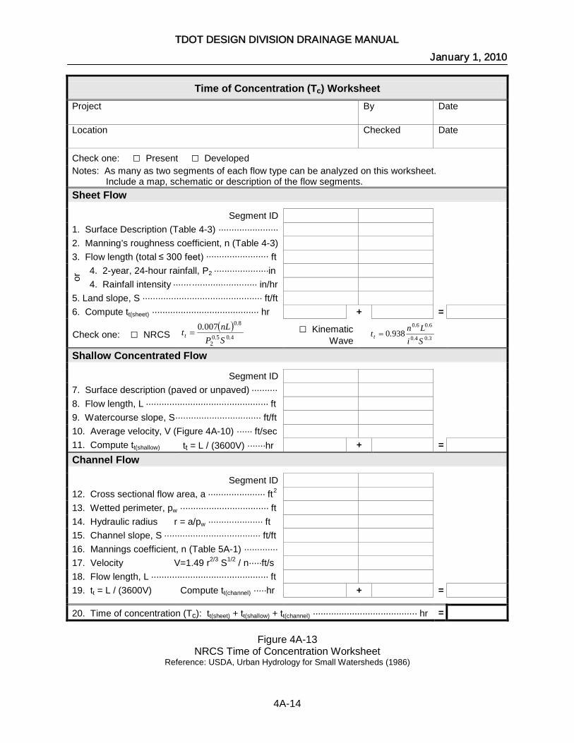
Once the designer has selected the rational method for determining design discharge, the following steps are applicable: Step 1: Determine drainage area. Step 2: Calculate runoff coefficient. Step 3: Find time of concentration. If the designer chooses the NRCS TR-55 Time of Concentration Method, a useful worksheet is included in the Appendix as Figure 4A-13. Step 4: Determine rainfall intensity. Step 5: Calculate storm runoff (design discharge). Step 6: Verify that any sub-area does not provide higher runoff.
Rational Method example problems are presented in the chapter Appendix. 4.04.2 USGS REGRESSION EQUATIONS FOR RURAL AREAS 4.04.2.1 BACKGROUND
The United States Geological Survey (USGS) published regression equations for rural
areas of Tennessee in 2003. The rural regression equation development is described in Water-Resources Investigations Report 03-4176, “Flood-Frequency Prediction Methods for Unregulated Streams of Tennessee, 2000”. The study was based on stream flow data gathered from 453 gauging stations located in rural and lightly developed areas of Tennessee and the adjacent states (except Arkansas). Of these, 297 gauges were located in Tennessee. All of the gauges had a minimum of 10 years of stream flow data. Stream gauges were not included in the analysis where historical discharge records had been significantly impacted by urbanization, dredging, or other man-made watershed changes.
A regional flood frequency analysis was conducted with these gauges and regional-
regression equations were developed based on a single variable, multivariable, and a region-of-influence method. For the single variable regression equations the contributing drainage area is used in predicting peak flow for the range of flood frequencies. The multiple variable regression equations add in the main channel slope and a climate factor in addition to the contributing drainage area in predicting peak flow for the range of flood frequencies. The region-of-influence method calculates multivariable regression equations using basin characteristics from 60 similar sites selected from the study area. The variables that may be used in the region-of-influence regression equations include contributing drainage area, main channel slope, a climate factor, and a physiographic-region factor.
Four hydrologically similar areas were identified during the regional flood frequency
analysis that improved the predictive capability of the regression equations. These four Hydrologic Areas are shown in Figure 4-3 and 4A-16. The single variable and multivariable regression equations for each of the four Hydrologic Areas of the state are shown in Table 4-4. The region-of-influence method is computationally intensive and is not suitable for manual application, however, it along with the other two methods can be easily applied using the

TDOT DESIGN DIVISION DRAINAGE MANUAL January 1, 2010
4-16
TDO
T - RO
AD
WA
Y DESIG
N G
UID
ELINES
English
Revised: 01/01/99
TDOTv203 computer application. In the absence of the flood-frequency computer application the single variable regression equations, shown in Table 4-4 should be used. The resulting flow in cubic feet per second can be obtained by using these equations.
The USGS regression equations should be applied to rural watercourses with drainage
area ranges shown in Table 4-5. The USGS methods were developed using stream-gauge records from unregulated streams draining basins having from 1 percent to about 30 percent total impervious area. These methods, however, should not be used in heavily developed or enclosed drainage system areas with impervious areas greater than 10 percent.
Recurrence Interval
Single Variable Regression Peak Discharge Equations
Multivariable Regression Peak Discharge Equations
(years) (cfs) (cfs) Hydrologic Area 1 (CDA = 128 ac to 9,000 mi2)
2 119(CDA)0.755 1.72(CDA)0.798 (CS)0.112 (CF)4.581
5 197(CDA)0.740 3.41(CDA)0.783 (CS)0.114 (CF)4.330
10 258(CDA)0.731 5.34(CDA)0.775 (CS)0.116 (CF)4.087
25 342(CDA)0.722 9.00(CDA)0.766 (CS)0.117 (CF)3.778
50 411(CDA)0.716 12.8(CDA)0.760 (CS)0.117 (CF)3.560
100 484(CDA)0.710 17.9(CDA)0.754 (CS)0.117 (CF)3.354
500 672(CDA)0.699 36.1(CDA)0.742 (CS)0.114 (CF)2.904 Hydrologic Area 2 (CDA = 300 ac to 2,557 mi2)
2 204(CDA)0.727 106(CDA)0.787 (CS)0.151
5 340(CDA)0.716 170(CDA)0.779 (CS)0.158
10 439(CDA)0.712 218(CDA)0.776 (CS)0.160
25 573(CDA)0.709 285(CDA)0.772 (CS)0.160
50 677(CDA)0.707 340(CDA)0.769 (CS)0.159
100 785(CDA)0.705 397(CDA)0.766 (CS)0.157
500 1,050(CDA)0.702 547(CDA)0.761 (CS)0.151 CDA is Contributing Drainage Area in square miles. CS is Channel Slope in feet per mile. CF is Climate Factor.
Table 4-4 (1 of 2) USGS Rural Regression Equations by Hydrologic Area
Reference: Flood-Frequency Prediction Methods for Unregulated Streams of Tennessee, 2000 Water-Resources Investigations Report 03-4176. USGS (2003)

TDOT DESIGN DIVISION DRAINAGE MANUAL January 1, 2010
4-17
TDO
T - RO
AD
WA
Y DESIG
N G
UID
ELINES
English
Revised: 01/01/99
Recurrence Interval
Single Variable Regression Peak Discharge Equations
Multivariable Regression Peak Discharge Equations
(years) (cfs) (cfs) Hydrologic Area 3 (CDA = 109 ac to 30.2 mi2)
2 280(CDA)0.789 211(CDA)0.815 (CS)0.063
5 452(CDA)0.769 329(CDA)0.798 (CS)0.071
10 574(CDA)0.761 405(CDA)0.793 (CS)0.078
25 733(CDA)0.753 497(CDA)0.789 (CS)0.086
50 853(CDA)0.748 565(CDA)0.786 (CS)0.092
100 972(CDA)0.745 632(CDA)0.785 (CS)0.096
500 1,250(CDA)0.739 789(CDA)0.781 (CS)0.102 Hydrologic Area 3 (CDA = 30.2 mi2 to 2,048 mi2)
2 679(CDA)0.527 409(CDA)0.584 (CS)0.102
5 1040(CDA)0.523 767(CDA)0.558 (CS)0.061
10 1280(CDA)0.523 980(CDA)0.554 (CS)0.054
25 1590(CDA)0.525 1,200(CDA)0.557 (CS)0.056
50 1800(CDA)0.527 1,330(CDA)0.562 (CS)0.061
100 2020(CDA)0.529 1,430(CDA)0.568 (CS)0.068
500 2490(CDA)0.537 1,600(CDA)0.587 (CS)0.090 Hydrologic Area 4 (CDA = 486 ac to 2,308 mi2)
2 436(CDA)0.527
No multivariable regression equations developed for this region.
5 618(CDA)0.545
10 735(CDA)0.554
25 878(CDA)0.564
50 981(CDA)0.570
100 1,080(CDA)0.575
500 1,310(CDA)0.586 CDA is Contributing Drainage Area in square miles. CS is Channel Slope in feet per mile. CF is Climate Factor.
Table 4-4 (2 of 2) USGS Rural Regression Equations by Hydrologic Area
Reference: Flood-Frequency Prediction Methods for Unregulated Streams of Tennessee, 2000 Water-Resources Investigations Report 03-4176. USGS (2003)

TDOT DESIGN DIVISION DRAINAGE MANUAL January 1, 2010
4-18
TDO
T - RO
AD
WA
Y DESIG
N G
UID
ELINES
English
Revised: 01/01/99
TDOT has determined that in most cases the Rational Method should be used for drainage areas less than 100 acres. The TR-55 Method should be used for rural drainage areas between 100 acres and the lower drainage area limit of the USGS rural regression equations for each Hydrologic Area shown in Table 4-5. The Natural Resources Conservation Service (NRCS) has developed a computer application called WinTR-55 for small watershed hydrology that can be used to apply the TR-55 method.
Hydrologic Area USGS Area Limits
1 128 ac to 9000 mi2 2 300 ac to 2557 mi2 3 109 ac to 30.2 mi2 4 486 ac to 2308 mi2
Table 4-5
USGS Rural Regression Equation Drainage Area Range Limitations Reference: Flood-Frequency Prediction Methods for Unregulated Streams of Tennessee, 2000
Water-Resources Investigations Report 03-4176. USGS (2003)

TDOT DESIGN DIVISION DRAINAGE MANUAL January 1, 2010
4-19
TDO
T - RO
AD
WA
Y DESIG
N G
UID
ELINES
English
Revised: 01/01/99
Figure 4-3 Hydrologic Area Map
(Note: Bold lines identify Hydrologic Area boundaries)

TDOT DESIGN DIVISION DRAINAGE MANUAL January 1, 2010
4-20
TDO
T - RO
AD
WA
Y DESIG
N G
UID
ELINES
English
Revised: 01/01/99
4.04.2.2 PROCEDURES 4.04.2.2.1 SINGLE VARIABLE REGRESSION EQUATIONS
The procedures for applying the single variable rural regression equations are described
in the following steps. The designer should follow these steps for all rural watersheds when the flood frequency computer application is not available.
Step 1: The designer determines the drainage area in acres using detailed project
mapping, surveys, and/or the USGS 7.5-minute topographic maps. Step 2: The designer determines in which Hydrologic Area the majority of the
watershed lies. A map of the Hydrologic Area boundaries is shown in Figure 4-3. Step 3: Select the appropriate regression equation based on the hydrologic area,
design frequency, and drainage area. Step 4: Compute the peak discharge using the appropriate regression equation for the
desired design frequency, drainage area, and hydrologic area. An example problem showing computations using the USGS single variable regression
equations for rural areas is included in the Appendix of this chapter.
4.04.2.2.2 FLOOD FREQUENCY COMPUTER APPLICATION The procedures for applying the single variable regression equations, multivariable
regression equations, and region-of-influence method are described in the following steps. The designer should follow these steps for all rural watersheds.
Step 1: Determine the latitude (LAT) and longitude (LNG), in degrees, minutes, and
seconds, of the site of interest. Step 2: Determine the hydrologic area(s) (HA) of the drainage basin upstream from the
site of interest. Step 3: Determine the contributing drainage area (CDA) in square miles, and the main
channel slope (CS), in feet per mile, of the site of interest using the best available information. If there are two HAs, determine the proportion of CDA that lies within each HA.
Step 4: Enter data from Steps 1 thru 3 into the TDOT v203 computer application. The
results will provide estimated discharges for the site of interest calculated based on the single regression equations, multivariable regression equations, and region-of-influence method. Use the estimated discharges from the method with the lowest standard error (SE). 4.04.3 USGS REGRESSION EQUATIONS FOR URBAN AREAS 4.04.3.1 BACKGROUND
The USGS developed regression equations for small urban streams of Tennessee in 1984. The process is described in Water-Resources Investigations Report 84-4182, “Synthesized Flood Frequency for Small Urban Streams in Tennessee”. Twenty-two streams

TDOT DESIGN DIVISION DRAINAGE MANUAL January 1, 2010
4-21
TDO
T - RO
AD
WA
Y DESIG
N G
UID
ELINES
English
Revised: 01/01/99
were studied statewide in urban areas with populations between 5,000 and 100,000. The drainage areas for these twenty-two sites ranged from 0.21 to 24.3 square miles. The impervious percentage in the watersheds for the study, ranged from 4.7 to 74.0 percent.
The stream flow record for the gages ranged from four to eight years. Due to the short record for the gages, rainfall-runoff models were calibrated for each of the watersheds. Flood magnitudes for selected recurrence intervals were then estimated for each of the watersheds using the calibrated models. These flood magnitudes were then used in a regional regression analysis to develop the regression equations. Three basin characteristics were determined to be significant in the regional regression analysis. These characteristics are drainage area, percent impervious, and the 2-year, 24-hour rainfall. The urban regression equations developed from this analysis are as follows: ( ) 013
242480740
2 640761 ..IMP
. PI/A.Q −= (4-11) ( ) 532
242440750
5 640555 ..IMP
. PI/A.Q −= (4-12) ( ) 122
242430750
10 640811 ..IMP
. PI/A.Q −= (4-13) ( ) 891
242390750
25 640921 ..IMP
. PI/A.Q −= (4-14) ( ) 421
242400750
50 640944 ..IMP
. PI/A.Q −= (4-15) ( ) 101
242400750
100 640077 ..IMP
. PI/A.Q −= (4-16) Where: Qr = estimated discharge for the recurrence interval indicated, (ft3/s) A = drainage area of the watershed, (acres) IIMP = percentage of impervious area in watershed, (%) P2-24 = 2-year, 24-hour rainfall, (inches) Note: The 2-year, 24-hour rainfall amounts for Tennessee counties are shown in Table 4A-5 found in the chapter Appendix. The USGS urban stream regression equations should be applied to all urban drainage areas greater than 100 acres. The impervious area for the watershed should be between 10 and 75 percent of the total watershed area. The stream flow should be unregulated. The peak flow magnitude should not be affected by in-channel storage or overbank detention storage. These equations should not be used in the City of Memphis or Shelby County. The USGS has developed regression equations specifically for urban watersheds in the City of Memphis and Shelby County. 4.04.3.2 PROCEDURES
The procedures for applying the urban regression equations are described in the following steps.

TDOT DESIGN DIVISION DRAINAGE MANUAL January 1, 2010
4-22
TDO
T - RO
AD
WA
Y DESIG
N G
UID
ELINES
English
Revised: 01/01/99
Step 1: The designer determines the drainage area in acres using the detailed project mapping and/or the USGS 7.5-minute topographic maps. Step 2: The designer determines the 2-year, 24-hour rainfall amount by from Table 4A-5. Projects located in more than one county shall use an interpolated value from the table. Step 3: Determine the amount of the impervious area in the watershed. The designer then computes the impervious percentage by dividing the impervious area by the total drainage area. Step 4: Compute the peak discharge using the appropriate regression equation for the desired frequency (see Equations 4-11 to 4-16).
USGS regression equation method example problem for urban areas is included in the chapter Appendix. 4.04.4 USGS REGRESSION EQUATIONS FOR THE CITY OF MEMPHIS AND SHELBY
COUNTY URBAN AREAS 4.04.4.1 BACKGROUND
A method for estimating the magnitude and frequency of peak discharges in the urban areas of the City of Memphis and Shelby County was developed by the USGS in 1984. The methodology development is described in Water-Resources Investigations Report 84-4110, “Flood Frequency and Storm Runoff of Urban Areas of Memphis and Shelby County, Tennessee.” The study was based on stream flow and rainfall records from 27 stream gauging stations and 37 rainfall gages. The drainage areas for the 27 gages ranged from 0.043 to 19.4 square miles.
Eight years of stream flow and rainfall records were gathered at the gages. This data
was used to calibrate a rainfall-runoff model for each gage for about 30 storms. The Lichty and Liscum map model procedure (1978) was used to develop peak discharge frequency curves for each of the gages using parameters optimized in the rainfall-runoff model calibration. These peak discharge frequency curves were used in a regional frequency analysis to identify physical basin characteristics that were significant in estimating peak flows. Two physical characteristics were identified in the regional frequency analysis as being significant predictors of peak flow rates. These basin characteristics are drainage area in square miles and channel condition. Channel condition represents how much of the channel at four points in the watershed is paved. 4.04.5 OTHER HYDROLOGIC METHODS 4.04.5.1 INTRODUCTION
This section presents other hydrologic methods that may be used by the designer when the preferred methods discussed previously are not applicable due to watershed conditions or where other hydrologic data is available for the stream crossing location. Examples of other hydrologic data are published peak flow rates from FEMA Flood Insurance Studies or other agencies. Hydrologic models utilizing hydrograph routing techniques may be required for some watersheds due to the presence of existing or proposed storage reservoirs. This section will discuss other sources of existing flow data and hydrologic models.

TDOT DESIGN DIVISION DRAINAGE MANUAL January 1, 2010
4-23
TDO
T - RO
AD
WA
Y DESIG
N G
UID
ELINES
English
Revised: 01/01/99
4.04.5.2 SOURCES OF EXISTING FLOW DATA
The designer should check for existing published flow data for the project site. A typical source of flow data is Federal Emergency Management Agency (FEMA) Flood Insurance Studies (FIS). These studies are generally published by FEMA for each community. As a minimum, the appropriate design storm published FIS flows should be used for the project site for the design of a structure. Other sources of existing flow data are stormwater management or flood control studies conducted by Federal, State, or local government agencies.
4.04.5.3 HYDROLOGIC MODELS INVOLVING DETENTION (HEC-1, HEC-HMS, AND TR-55)
The hydrologic models and methods described in this section are to be used by the designer when detention storage will be included in the highway drainage design or for watersheds where the rational method or regression equations are not applicable. These methods should also be used for watersheds that have significant existing reservoir storage, diversions, and other significant man-made changes that have made TDOT preferred hydrologic methods inapplicable to the watershed. The hydrologic models for this purpose are the U.S. Army Corps of Engineers' HEC-1 and HEC-HMS and the Natural Resource Conservation Service's TR-55. When using one of these models, the designer should be familiar with hydrologic modeling concepts.
HEC-1 and HEC-HMS are more versatile and provide a wider variety of modeling
techniques for watershed features. The user’s manuals for these models should be consulted for the specifics on how to use the models and the data input requirements. Additional information on the routing capabilities of these programs can be found in Chapter 8 of this Manual. 4.04.5.3.1 HYDROLOGIC MODEL LOSS RATE AND UNIT HYDROGRAPH METHODOLOGY
The SCS curve number loss rate and unit hydrograph methodology are the preferred methods to be used by the designer in computing runoff hydrographs in HEC-1, HEC-HMS, and TR-55. The SCS TR-55 time of concentration methodology described in Section 4.04.1.3 should be used by the designer. The following paragraphs describe the methodology for determining the SCS curve number for a watershed.
The principle factors that determine the Runoff Curve Number (CN) are the hydrologic soil group, ground cover type, treatment, hydrologic condition, antecedent runoff condition, and how the flow enters the drainage system. This design methodology assumes that the runoff potential before a storm event is at "average" conditions. This pre-storm runoff potential is also described as the Antecedent Runoff Condition. Tables 4A-1 to 4A-3 found in the Appendix list runoff curve numbers for various land uses and hydrologic soil groups. A worksheet for determining the composite runoff curve number and runoff is included in the Appendix as Figure 4A-14.
In determining the curve number, soils are classified into four hydrologic soil groups (A, B, C, and D). The classifications are based on bare soil infiltration rates after prolonged wetting. The infiltration rates are affected by subsurface permeability and surface intake rates. The soils in the project or study area can be identified from a soil survey report which can be obtained from a soil and water conservation district office or local National Resource Conservation Service office. A summary of common Hydrologic Soil Groups found in Tennessee are included

TDOT DESIGN DIVISION DRAINAGE MANUAL January 1, 2010
4-24
TDO
T - RO
AD
WA
Y DESIG
N G
UID
ELINES
English
Revised: 01/01/99
in Table 4A-4 found in the chapter appendix. If the soil group is not included in Table 4A-4, then the designer should refer to the TR-55 document referenced in Table 4A-1.
Even though urban areas have more impervious areas (i.e., buildings, roadways, and,
sidewalks) than rural areas, soil remains an important factor in estimating the amount of runoff. According to TR-55, "Urbanization has a greater effect on runoff in watersheds with soils having high infiltration rates (sands and gravels) than in watersheds predominantly of silts and clays, which generally have low infiltration rates." The designer should be aware that natural soils may have been disturbed by prior projects. Native soils may be mixed with soils introduced from other areas (fill material) or may be removed (excavation). Hydrologic Soil Groups for disturbed soils can be characterized by the soil texture as identified in Table 4-7.
Hydrologic Soil
Group (HSG) Soil Textures
A Sand, loamy sand, or sandy loam
B Silt loam or loam
C Sandy clay loam
D Clay loam, silty clay loam, sandy clay, silty clay, or clay
Table 4-6 Hydrologic Soil Groups for Disturbed Soils Reference: NRCS, TR-55, Second Edition (1986)
Tables 4A-1 to 4A-3 address the most common ground cover types. The preferred
method for determining the type of ground cover is from field reconnaissance. Aerial photography and land use maps are also useful sources.
Ground Treatment describes a modification to the ground cover made by management practices on agricultural land. The treatments are bare soil, crop residue cover, straight row, contoured, and contoured & terraced. These are each identified in Table 4A-2.
The hydrologic condition indicates the effects of the ground cover and any given ground treatment on runoff and water infiltration. The hydrologic condition is generally classified as either "good" or "poor." "Good" hydrologic conditions indicate that the soil would have low runoff potential. According to the NRCS, the designer should consider five factors when estimating the effect of the cover on infiltration and runoff:
• Density of lawns, crops, or other vegetative areas • Amount of year-round cover • Amount of grass or close-seeded legumes in rotations • Percent of residue cover • Degree of surface roughness
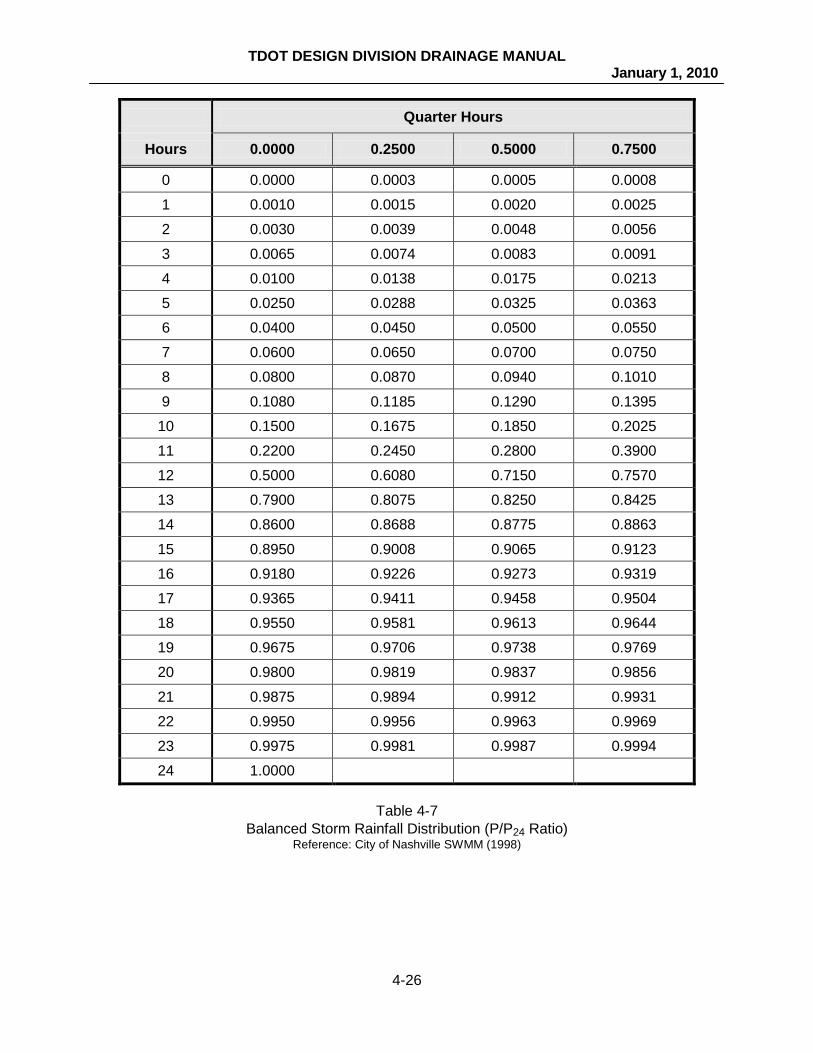
4.04.5.3.2 RAINFALL DISTRIBUTIONS
The 24-hour rainfall amounts (in inches) for the desired design frequency are available in the NWS Rainfall Atlas 14, Volume 2 and are included in the chapter appendix as Tables 4A-5 to 4A-10. A balanced rainfall distribution should be used by the designer. A balanced rainfall

TDOT DESIGN DIVISION DRAINAGE MANUAL January 1, 2010
4-25
TDO
T - RO
AD
WA
Y DESIG
N G
UID
ELINES
English
Revised: 01/01/99
distribution is where the greatest rainfall intensity occurs during the central portion of the storm. The tabulated balanced storm distribution is shown in Table 4-10 and plotted graphically as Figure 4A-15 in the Appendix. For analysis with TR-55 or HEC-HMS, the NRCS Type II rainfall distribution, which is pre-coded into both programs, may be used.
TDOT DESIGN DIVISION DRAINAGE MANUAL January 1, 2010
4-26
TDO
T - RO
AD
WA
Y DESIG
N G
UID
ELINES
English
Revised: 01/01/99
Quarter Hours
Hours 0.0000 0.2500 0.5000 0.7500
0 0.0000 0.0003 0.0005 0.0008
1 0.0010 0.0015 0.0020 0.0025
2 0.0030 0.0039 0.0048 0.0056
3 0.0065 0.0074 0.0083 0.0091
4 0.0100 0.0138 0.0175 0.0213
5 0.0250 0.0288 0.0325 0.0363
6 0.0400 0.0450 0.0500 0.0550
7 0.0600 0.0650 0.0700 0.0750
8 0.0800 0.0870 0.0940 0.1010
9 0.1080 0.1185 0.1290 0.1395
10 0.1500 0.1675 0.1850 0.2025
11 0.2200 0.2450 0.2800 0.3900
12 0.5000 0.6080 0.7150 0.7570
13 0.7900 0.8075 0.8250 0.8425
14 0.8600 0.8688 0.8775 0.8863
15 0.8950 0.9008 0.9065 0.9123
16 0.9180 0.9226 0.9273 0.9319
17 0.9365 0.9411 0.9458 0.9504
18 0.9550 0.9581 0.9613 0.9644
19 0.9675 0.9706 0.9738 0.9769
20 0.9800 0.9819 0.9837 0.9856
21 0.9875 0.9894 0.9912 0.9931
22 0.9950 0.9956 0.9963 0.9969
23 0.9975 0.9981 0.9987 0.9994
24 1.0000
Table 4-7 Balanced Storm Rainfall Distribution (P/P24 Ratio)
Reference: City of Nashville SWMM (1998)

TDOT DESIGN DIVISION DRAINAGE MANUAL January 1, 2010
4-27
TDO
T - RO
AD
WA
Y DESIG
N G
UID
ELINES
English
Revised: 01/01/99
SECTION 4.05 - ACCEPTABLE SOFTWARE
The hydrology software listed in this section is acceptable for use on all TDOT projects. This software should be used unless special circumstances on the project or watershed require other software. The TDOT design manager should approve the use of any other software for these special circumstances. The acceptable software is listed in Table 4-11.
Under special circumstances, the designer will need to compute peak flow rates from mostly impervious areas or generate runoff hydrographs for the design of detention facilities, or determining peak flow rates from upstream reservoirs. When a runoff hydrograph is required, the designer should use either the Corps of Engineers HEC-HMS, or NRCS TR-55 hydrologic models. The Corps of Engineers HEC-1 model may be used only if there is an existing HEC-1 model.
The National Flood Frequency program is published by the United States Geological
Survey and is available on the internet. The results of this program should be consistent with the current USGS regression equations for both rural and urban areas. The user should verify that results obtained from this program are consistent with the regression equations presented in this manual.
Approved Software Uses
GeoPak Computes Peak Discharge
Rational Method NRCS Curve Number Method
National Flood Frequency Program, USGS StreamStats,
TDOTv2.0.3
Computes Peak Discharge USGS Rural Regression Equation USGS Urban Regression Equation
USGS Memphis Regression Equation
HEC-HMS, HEC-1 *
Develops Hydrographs using NRCS Curve Number and Unit Hydrograph Methods
Channel Routings Reservoir Routings (existing and proposed)
Diversions
TR-55
Develops Hydrographs using NRCS Curve Number and Unit Hydrograph Methods
Channel Routings Reservoir Routings (existing and proposed)
Diversions * HEC-1 may be used only if there is an existing HEC-1 model
Table 4-8 Acceptable Computer Software
TDOT DESIGN DIVISION
DRAINAGE MANUAL
CHAPTER IV APPENDIX 4A

TDOT DESIGN DIVISION DRAINAGE MANUAL January 1, 2010
4A-1
SECTION 4.06 - APPENDIX
4.06.1 FIGURES AND TABLES

TDOT DESIGN DIVISION DRAINAGE MANUAL January 1, 2010
4A-2
Figu
re 4
A-1
IDF
Zone
Loc
atio
n M
ap

TDOT DESIGN DIVISION DRAINAGE MANUAL January 1, 2010
4A-3
Duration
Rai
nfal
l Int
ensi
ty (i
n/hr
)
5 10 15 30 60 2 3 6 12 24
0.10
1.0
10.0
15.0
20 40 450 5Minutes Hours
8 10 18
20.0
8.0
6.0
4.0
2.0
0.8
0.6
0.4
0.2
0.08
0.06
0.04
0.02
Return Period:2-Year5-Year10-Year25-Year50-Year100-Year
Figure 4A-2 Chattanooga IDF Curve
NOTE: Tc = 5 minutes is a minimum value to use in all cases Reference: National Weather Service, NOAA Atlas 14, Volume 2 (2004)

TDOT DESIGN DIVISION DRAINAGE MANUAL January 1, 2010
4A-4
Duration
Rai
nfal
l Int
ensi
ty (i
n/hr
)
5 10 15 30 60 2 3 6 12 24
0.10
1.0
10.0
15.0
20 40 450 5Minutes Hours
8 10 18
20.0
8.0
6.0
4.0
2.0
0.8
0.6
0.4
0.2
0.08
0.06
0.04
0.02
Return Period:2-Year5-Year10-Year25-Year50-Year100-Year
Figure 4A-3 Clarksville IDF Curve
NOTE: Tc = 5 minutes is a minimum value to use in all cases Reference: National Weather Service, NOAA Atlas 14, Volume 2 (2004)

TDOT DESIGN DIVISION DRAINAGE MANUAL January 1, 2010
4A-5
Duration
Rai
nfal
l Int
ensi
ty (i
n/hr
)
5 10 15 30 60 2 3 6 12 24
0.10
1.0
10.0
15.0
20 40 450 5Minutes Hours
8 10 18
20.0
8.0
6.0
4.0
2.0
0.8
0.6
0.4
0.2
0.08
0.06
0.04
0.02
Return Period:2-Year5-Year10-Year25-Year50-Year100-Year
Figure 4A-4 Cookeville IDF Curve
NOTE: Tc = 5 minutes is a minimum value to use in all cases Reference: National Weather Service, NOAA Atlas 14, Volume 2 (2004)

TDOT DESIGN DIVISION DRAINAGE MANUAL January 1, 2010
4A-6
Duration
Rai
nfal
l Int
ensi
ty (i
n/hr
)
5 10 15 30 60 2 3 6 12 24
0.10
1.0
10.0
15.0
20 40 450 5Minutes Hours
8 10 18
20.0
8.0
6.0
4.0
2.0
0.8
0.6
0.4
0.2
0.08
0.06
0.04
0.02
Return Period:2-Year5-Year10-Year25-Year50-Year100-Year
Figure 4A-5 Jackson IDF Curve
NOTE: Tc = 5 minutes is a minimum value to use in all cases Reference: National Weather Service, NOAA Atlas 14, Volume 2 (2004)

TDOT DESIGN DIVISION DRAINAGE MANUAL January 1, 2010
4A-7
Duration
Rai
nfal
l Int
ensi
ty (i
n/hr
)
5 10 15 30 60 2 3 6 12 24
0.10
1.0
10.0
15.0
20 40 450 5Minutes Hours
8 10 18
20.0
8.0
6.0
4.0
2.0
0.8
0.6
0.4
0.2
0.08
0.06
0.04
0.02
Return Period:2-Year5-Year10-Year25-Year50-Year100-Year
Figure 4A-6 Johnson City IDF Curve
NOTE: Tc = 5 minutes is a minimum value to use in all cases Reference: National Weather Service, NOAA Atlas 14, Volume 2 (2004)
TDOT DESIGN DIVISION DRAINAGE MANUAL January 1, 2010
4A-8
Duration
Rai
nfal
l Int
ensi
ty (i
n/hr
)
5 10 15 30 60 2 3 6 12 24
0.10
1.0
10.0
15.0
20 40 450 5Minutes Hours
8 10 18
20.0
8.0
6.0
4.0
2.0
0.8
0.6
0.4
0.2
0.08
0.06
0.04
0.02
Return Period:2-Year5-Year10-Year25-Year50-Year100-Year
Figure 4A-7 Knoxville IDF Curve
NOTE: Tc = 5 minutes is a minimum value to use in all cases Reference: National Weather Service, NOAA Atlas 14, Volume 2 (2004)

TDOT DESIGN DIVISION DRAINAGE MANUAL January 1, 2010
4A-9
Duration
Rai
nfal
l Int
ensi
ty (i
n/hr
)
5 10 15 30 60 2 3 6 12 24
0.10
1.0
10.0
15.0
20 40 450 5Minutes Hours
8 10 18
20.0
8.0
6.0
4.0
2.0
0.8
0.6
0.4
0.2
0.08
0.06
0.04
0.02
Return Period:2-Year5-Year10-Year25-Year50-Year100-Year
Figure 4A-8 Lawrenceburg IDF Curve
NOTE: Tc = 5 minutes is a minimum value to use in all cases Reference: National Weather Service, NOAA Atlas 14, Volume 2 (2004)

TDOT DESIGN DIVISION DRAINAGE MANUAL January 1, 2010
4A-10
Duration
Rai
nfal
l Int
ensi
ty (i
n/hr
)
5 10 15 30 60 2 3 6 12 24
0.10
1.0
10.0
15.0
20 40 450 5Minutes Hours
8 10 18
20.0
8.0
6.0
4.0
2.0
0.8
0.6
0.4
0.2
0.08
0.06
0.04
0.02
Return Period:2-Year5-Year10-Year25-Year50-Year100-Year
Figure 4A-9 Lebanon IDF Curve
NOTE: Tc = 5 minutes is a minimum value to use in all cases Reference: National Weather Service, NOAA Atlas 14, Volume 2 (2004)

TDOT DESIGN DIVISION DRAINAGE MANUAL January 1, 2010
4A-11
Duration
Rai
nfal
l Int
ensi
ty (i
n/hr
)
5 10 15 30 60 2 3 6 12 24
0.10
1.0
10.0
15.0
20 40 450 5Minutes Hours
8 10 18
20.0
8.0
6.0
4.0
2.0
0.8
0.6
0.4
0.2
0.08
0.06
0.04
0.02
Return Period:2-Year5-Year10-Year25-Year50-Year100-Year
Figure 4A-10 Manchester IDF Curve
NOTE: Tc = 5 minutes is a minimum value to use in all cases Reference: National Weather Service, NOAA Atlas 14, Volume 2 (2004)

TDOT DESIGN DIVISION DRAINAGE MANUAL January 1, 2010
4A-12
Duration
Rai
nfal
l Int
ensi
ty (i
n/hr
)
5 10 15 30 60 2 3 6 12 24
0.10
1.0
10.0
15.0
20 40 450 5Minutes Hours
8 10 18
20.0
8.0
6.0
4.0
2.0
0.8
0.6
0.4
0.2
0.08
0.06
0.04
0.02
Return Period:2-Year5-Year10-Year25-Year50-Year100-Year
Figure 4A-11 Shelbyville IDF Curve
NOTE: Tc = 5 minutes is a minimum value to use in all cases Reference: National Weather Service, NOAA Atlas 14, Volume 2 (2004)

TDOT DESIGN DIVISION DRAINAGE MANUAL January 1, 2010
4A-13
Figure 4A-12 Shallow Concentrated Flow Average Velocities
Reference: USDA, Urban Hydrology for Small Watersheds (1986)
TDOT DESIGN DIVISION DRAINAGE MANUAL January 1, 2010
4A-14
Time of Concentration (Tc) Worksheet Project By Date
Location Checked Date
Check one: □ Present □ Developed Notes: As many as two segments of each flow type can be analyzed on this worksheet. Include a map, schematic or description of the flow segments. Sheet Flow
Segment ID
1. Surface Description (Table 4-3) ······················· 2. Manning’s roughness coefficient, n (Table 4-3) 3. Flow length (total ≤ 300 feet) ∙∙∙∙∙∙∙∙∙∙∙∙∙∙∙∙∙∙∙∙∙∙∙∙ ft
or 4. 2-year, 24-hour rainfall, P2 ·····················in
4. Rainfall intensity ······· ························· in/hr 5. Land slope, S ·············································· ft/ft 6. Compute tt(sheet) ········································· hr + =
Check one: □ NRCS ( )
40502
800070..
.
t SPnL.t = □ Kinematic
Wave 3040
60609380
..
..
t SiLn.t =
Shallow Concentrated Flow
Segment ID 7. Surface description (paved or unpaved) ·········· 8. Flow length, L ··············································· ft 9. Watercourse slope, S································· ft/ft 10. Average velocity, V (Figure 4A-10) ······ ft/sec 11. Compute tt(shallow) tt = L / (3600V) ·······hr + =
Channel Flow Segment ID
12. Cross sectional flow area, a ······················ ft2 13. Wetted perimeter, pw ·································· ft 14. Hydraulic radius r = a/pw ····················· ft 15. Channel slope, S ····································· ft/ft 16. Mannings coefficient, n (Table 5A-1) ············· 17. Velocity V=1.49 r2/3 S1/2 / n·····ft/s 18. Flow length, L ············································· ft 19. tt = L / (3600V) Compute tt(channel) ·····hr + =
20. Time of concentration (Tc): tt(sheet) + tt(shallow) + tt(channel) ········································ hr =
Figure 4A-13
NRCS Time of Concentration Worksheet Reference: USDA, Urban Hydrology for Small Watersheds (1986)

TDOT DESIGN DIVISION DRAINAGE MANUAL January 1, 2010
4A-15
Curve Number Computation Worksheet Project By Date
Location Checked Date
Check one: □ Present □ Developed
Soil Name and Hydrologic Group (see Table 4A-4)
Cover Description: Curve Number1 Area
(cover type, treatment and hydrologic condition; % impervious; unconnected or
connected impervious area ratio)
Tabl
e 4A
-1
Tabl
e 4A
-2
Tabl
e 4A
-3
□ ac. □ mi2
□ %
Product of CN x
Area
1 Use only one CN source per line TOTALS:
USE CN =
Figure 4A-14 Curve Number Worksheet
Reference: USDA, Urban Hydrology for Small Watersheds (1986)
( ) _______areatotal
producttotalweightedCN ===

TDOT DESIGN DIVISION DRAINAGE MANUAL January 1, 2010
4A-16
Rainfall Ratio
0 0.1 0.2 0.3 0.4 0.5 0.6 0.7 0.8 0.9 1 0
2
4
6
8
10
12
14
16
18
20
22
24
TIM
E (h
ours
)
Figu
re 4
A-15
Ba
lanc
ed S
torm
Rai
nfal
l Dis
tribu
tion
(P/P
24 R
atio
)

TDOT DESIGN DIVISION DRAINAGE MANUAL January 1, 2010
4A-17
Figure 4A-16 Tennessee Physiographic Regions
Reference: Adapted from USGS, 2003
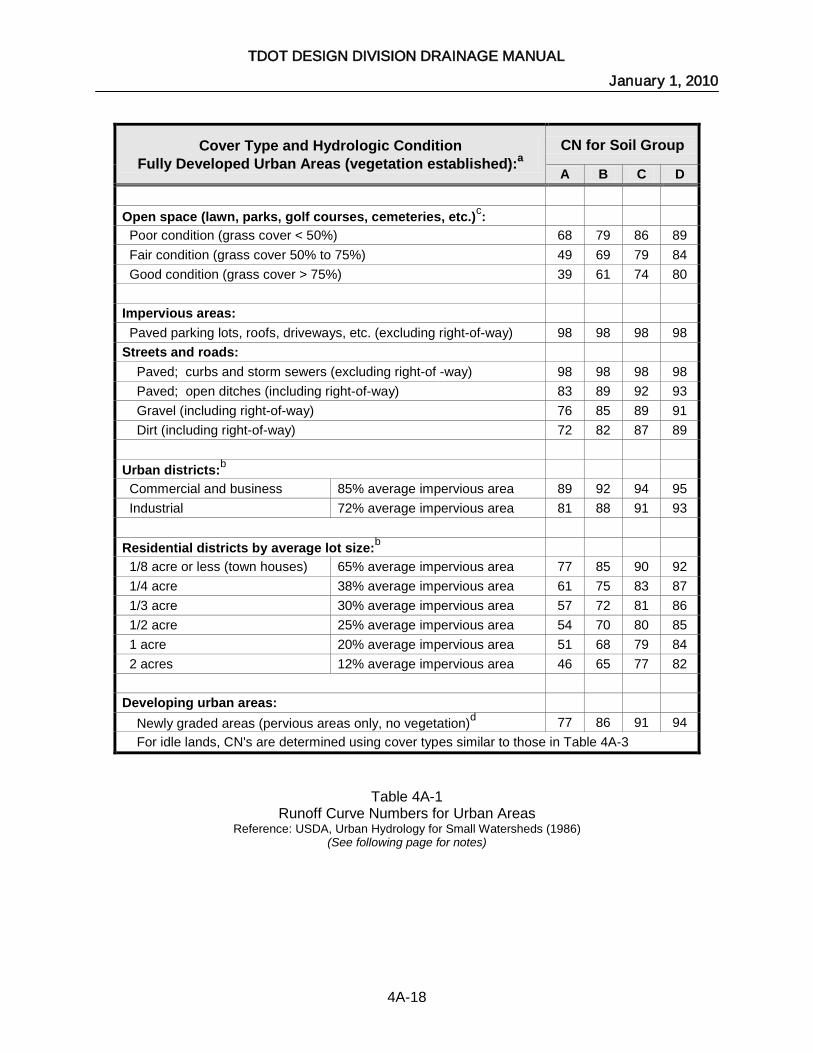
TDOT DESIGN DIVISION DRAINAGE MANUAL January 1, 2010
4A-18
Cover Type and Hydrologic Condition Fully Developed Urban Areas (vegetation established):a
CN for Soil Group
A B C D Open space (lawn, parks, golf courses, cemeteries, etc.)c: Poor condition (grass cover < 50%) 68 79 86 89 Fair condition (grass cover 50% to 75%) 49 69 79 84 Good condition (grass cover > 75%) 39 61 74 80 Impervious areas: Paved parking lots, roofs, driveways, etc. (excluding right-of-way) 98 98 98 98 Streets and roads: Paved; curbs and storm sewers (excluding right-of -way) 98 98 98 98 Paved; open ditches (including right-of-way) 83 89 92 93 Gravel (including right-of-way) 76 85 89 91 Dirt (including right-of-way) 72 82 87 89 Urban districts:b Commercial and business 85% average impervious area 89 92 94 95 Industrial 72% average impervious area 81 88 91 93 Residential districts by average lot size:b 1/8 acre or less (town houses) 65% average impervious area 77 85 90 92 1/4 acre 38% average impervious area 61 75 83 87 1/3 acre 30% average impervious area 57 72 81 86 1/2 acre 25% average impervious area 54 70 80 85 1 acre 20% average impervious area 51 68 79 84 2 acres 12% average impervious area 46 65 77 82 Developing urban areas: Newly graded areas (pervious areas only, no vegetation)d 77 86 91 94 For idle lands, CN's are determined using cover types similar to those in Table 4A-3
Table 4A-1 Runoff Curve Numbers for Urban Areas
Reference: USDA, Urban Hydrology for Small Watersheds (1986) (See following page for notes)

TDOT DESIGN DIVISION DRAINAGE MANUAL January 1, 2010
4A-19
aAverage runoff condition and I = 0.2S bThe average percent impervious area shown was used to develop the composite CN’s. Other assumptions are as follows: impervious areas are directly connected to the drainage system, impervious areas have a CN of 98, and pervious areas are considered equivalent to open space in good hydrologic condition. CN’s for other combinations of conditions may be computed using methods described in TR 55. cCNs shown are equivalent to those of pasture. Composite CN’s may be computed for other combinations of open space cover type. dComposite CN’s to use for the design of temporary measures during grading and construction should be computed based on the degree of development (impervious area percentage) and the CN’s for the newly graded pervious areas. Table References: American Association of State Highway and Transportation Officials. Model Drainage Manual [Metric Edition]. Washington, D.C. 1999. Metropolitan Government of Nashville and Davidson County Department of Public Works Engineering Division. Stormwater Management Manual. Nashville, Tennessee. Sept. 1999. United States Department of Agriculture. Soil Conservation Service. Engineering Division. Urban Hydrology for Small Watersheds - Technical Release 55. June 1986 (available for download at http://www.wcc.nrcs.usda.gov/water/quality/common/tr55/tr55.html).
Table 4A-1 (continued)
Runoff Curve Numbers for Urban Areas Reference: USDA, Urban Hydrology for Small Watersheds (1986)

TDOT DESIGN DIVISION DRAINAGE MANUAL January 1, 2010
4A-20
Cover Descriptiona Hydrologic
Conditionc CN for Soil Group
Cover type Treatmentb A B C D
Fallow Bare soil ----- 77 86 91 94
Crop residue cover (CR) Poor 76 85 90 93 Good 74 83 88 90
Row crops
Straight row (SR) Poor 72 81 88 91 Good 67 78 85 89
SR + CR Poor 71 80 87 90 Good 64 75 82 85
Contoured (C) Poor 70 79 84 88 Good 65 75 82 86
C + CR Poor 69 78 83 87 Good 64 74 81 85
Contoured & terraced (C&T)
Poor 66 74 80 82 Good 62 71 78 81
C&T + CR Poor 65 73 79 81 Good 61 70 77 80
Small grain
SR Poor 65 76 84 88 Good 63 75 83 87
SR + CR Poor 64 75 83 86 Good 60 72 80 84
C Poor 63 74 82 85 Good 61 73 81 84
C +CR Poor 62 73 81 84 Good 60 72 80 83
C&T Poor 61 72 79 82 Good 59 70 78 81
C&T + CR Poor 60 71 78 81 Good 58 69 77 80
Close-seeded or broadcast legumes or rotation meadow
SR Poor 66 77 85 89 Good 58 72 81 85
C Poor 64 75 83 85 Good 55 69 78 83
C&T Poor 63 73 80 83 Good 51 67 76 80
Table 4A-2
Runoff Curve Numbers for Cultivated Agricultural Landsa
Reference: USDA, Urban Hydrology for Small Watersheds (1986) (See following page for notes)

TDOT DESIGN DIVISION DRAINAGE MANUAL January 1, 2010
4A-21
aAverage runoff condition, I = 0.2S bCrop residue cover applies only if residue is on at least 5% of the surface throughout the year cHydraulic condition is based on combination factors that affect infiltration and runoff, including a.) density and canopy of vegetative areas b.) amount of year-round cover c.) amount of grass or close seeded legumes d.) percent of residue cover on the land surface (good > 20%) e.) degree of surface roughness Poor: Factors impair infiltration and tend to increase runoff Good: Factors encourage average and better than average infiltration and tend to decrease runoff Table References: American Association of State Highway and Transportation Officials. Model Drainage Manual [Metric Edition]. Washington, D.C. 1999. Metropolitan Government of Nashville and Davidson County Department of Public Works Engineering Division. Stormwater Management Manual. Nashville, Tennessee. Sept. 1999. United States Department of Agriculture. Soil Conservation Service. Engineering Division. Urban Hydrology for Small Watersheds - Technical Release 55. June 1986 (available for download at http://www.wcc.nrcs.usda.gov/water/quality/common/tr55/tr55.html).
Table 4A-2 (continued) Runoff Curve Numbers for Cultivated Agricultural Lands
Reference: USDA, Urban Hydrology for Small Watersheds (1986)

TDOT DESIGN DIVISION DRAINAGE MANUAL January 1, 2010
4A-22
Cover Type and Description Hydrologic Condition
CN for Soil Group A B C D
Pasture, grassland, or range--continuous forage for grazingb
Poor 68 79 86 89 Fair 49 69 79 84
Good 39 61 74 80 Meadow--continuous grass, protected from grazing and generally mowed for hay ---- 30 58 71 78
Brush--brush-weed-grass mixture with brush the major elementc
Poor 48 67 77 83 Fair 35 56 70 77
Good 30d 48 65 73 Woods--grass combination (orchard or tree farm)e
Poor 57 73 82 86 Fair 43 65 76 82
Good 32 58 72 79
Woodsf Poor 45 66 77 83 Fair 36 60 73 79
Good 30d 55 70 77 Farmsteads--buildings, lanes, driveways, and surrounding lots ---- 59 74 82 86
Table 4A-3 Runoff Curve Numbers For Rural Areas and Other Agricultural Landsa
Reference: USDA, Urban Hydrology for Small Watersheds (1986) (See following page for notes)
aAverage runoff condition, and I = 0.2S. bPoor: <50% ground cover or heavily grazed with no mulch. Fair: 50 to 75% ground cover and not heavily grazed. Good: >75% ground cover and lightly or only occasionally grazed. cPoor: <50% ground cover. Fair: 50 to 75% ground cover. Good: > 75% ground cover. dActual curve number is less than 30; use CN = 30 for runoff computations. eCN’s shown were computed for areas with 50% woods and 50% grass (pasture) cover. Other combinations of conditions may be computed from CN’s for woods and pasture. fPoor: Forest litter, small trees, and brush are destroyed by heavy grazing or regular burning. Fair: Woods are grazed but not burned, and some forest litter covers the soil.

TDOT DESIGN DIVISION DRAINAGE MANUAL January 1, 2010
4A-23
Good: Woods are protected from grazing and litter and brush adequately cover the soil. Table References: American Association of State Highway and Transportation Officials. Model Drainage Manual [Metric Edition]. Washington, D.C. 1999. Metropolitan Government of Nashville and Davidson County Department of Public Works Engineering Division. Stormwater Management Manual. Nashville, Tennessee. Sept. 1999. United States Department of Agriculture. Soil Conservation Service. Engineering Division. Urban Hydrology for Small Watersheds - Technical Release 55. June 1986 (available for download at http://www.wcc.nrcs.usda.gov/water/quality/common/tr55/tr55.html)
Table 4A-3 (continued) Runoff Curve Numbers For Rural Areas and Other Agricultural Lands
Reference: USDA, Urban Hydrology for Small Watersheds (1986)
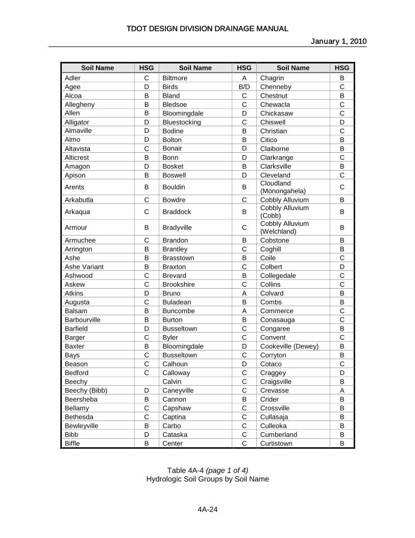
TDOT DESIGN DIVISION DRAINAGE MANUAL January 1, 2010
4A-24
Soil Name HSG Soil Name HSG Soil Name HSG
Adler C Biltmore A Chagrin B Agee D Birds B/D Chenneby C Alcoa B Bland C Chestnut B Allegheny B Bledsoe C Chewacla C Allen B Bloomingdale D Chickasaw C Alligator D Bluestocking C Chiswell D Almaville D Bodine B Christian C Almo D Bolton B Citico B Altavista C Bonair D Claiborne B Alticrest B Bonn D Clarkrange C Amagon D Bosket B Clarksville B Apison B Boswell D Cleveland C
Arents B Bouldin B Cloudland (Monongahela) C
Arkabutla C Bowdre C Cobbly Alluvium B
Arkaqua C Braddock B Cobbly Alluvium (Cobb) B
Armour B Bradyville C Cobbly Alluvium (Welchland) B
Armuchee C Brandon B Cobstone B Arrington B Brantley C Coghill B Ashe B Brasstown B Coile C Ashe Variant B Braxton C Colbert D Ashwood C Brevard B Collegedale C Askew C Brookshire C Collins C Atkins D Bruno A Colvard B Augusta C Buladean B Combs B Balsam B Buncombe A Commerce C Barbourville B Burton B Conasauga C Barfield D Busseltown C Congaree B Barger C Byler C Convent C Baxter B Bloomingdale D Cookeville (Dewey) B Bays C Busseltown C Corryton B Beason C Calhoun D Cotaco C Bedford C Calloway C Craggey D Beechy Calvin C Craigsville B Beechy (Bibb) D Caneyville C Crevasse A Beersheba B Cannon B Crider B Bellamy C Capshaw C Crossville B Bethesda C Captina C Cullasaja B Bewleyville B Carbo C Culleoka B Bibb D Cataska C Cumberland B Biffle B Center C Curtistown B
Table 4A-4 (page 1 of 4) Hydrologic Soil Groups by Soil Name
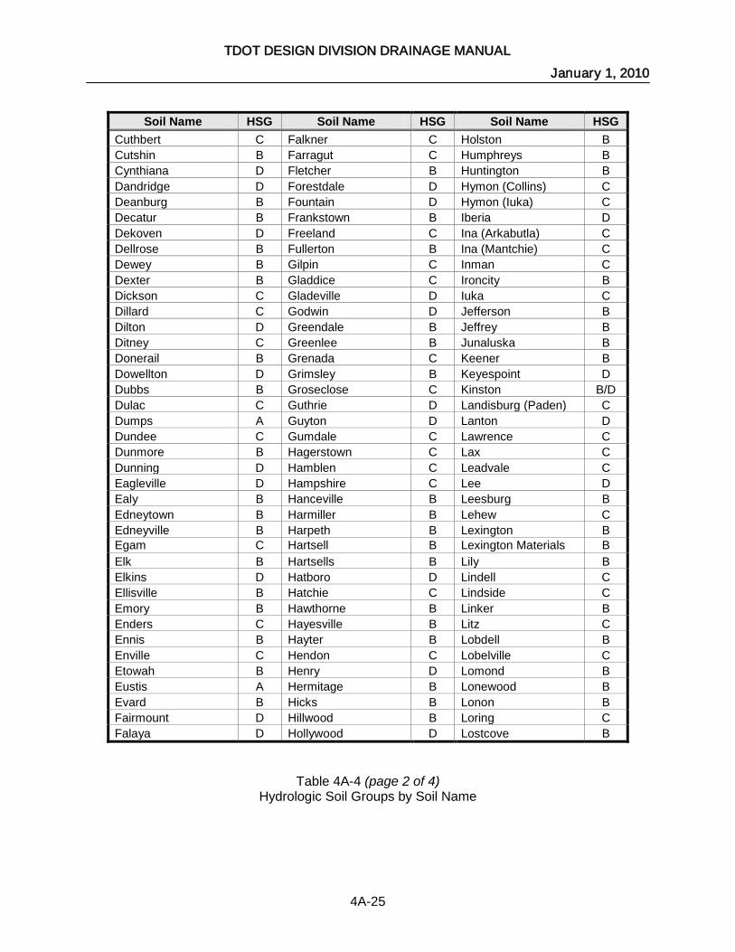
TDOT DESIGN DIVISION DRAINAGE MANUAL January 1, 2010
4A-25
Soil Name HSG Soil Name HSG Soil Name HSG
Cuthbert C Falkner C Holston B Cutshin B Farragut C Humphreys B Cynthiana D Fletcher B Huntington B Dandridge D Forestdale D Hymon (Collins) C Deanburg B Fountain D Hymon (Iuka) C Decatur B Frankstown B Iberia D Dekoven D Freeland C Ina (Arkabutla) C Dellrose B Fullerton B Ina (Mantchie) C Dewey B Gilpin C Inman C Dexter B Gladdice C Ironcity B Dickson C Gladeville D Iuka C Dillard C Godwin D Jefferson B Dilton D Greendale B Jeffrey B Ditney C Greenlee B Junaluska B Donerail B Grenada C Keener B Dowellton D Grimsley B Keyespoint D Dubbs B Groseclose C Kinston B/D Dulac C Guthrie D Landisburg (Paden) C Dumps A Guyton D Lanton D Dundee C Gumdale C Lawrence C Dunmore B Hagerstown C Lax C Dunning D Hamblen C Leadvale C Eagleville D Hampshire C Lee D Ealy B Hanceville B Leesburg B Edneytown B Harmiller B Lehew C Edneyville B Harpeth B Lexington B Egam C Hartsell B Lexington Materials B Elk B Hartsells B Lily B Elkins D Hatboro D Lindell C Ellisville B Hatchie C Lindside C Emory B Hawthorne B Linker B Enders C Hayesville B Litz C Ennis B Hayter B Lobdell B Enville C Hendon C Lobelville C Etowah B Henry D Lomond B Eustis A Hermitage B Lonewood B Evard B Hicks B Lonon B Fairmount D Hillwood B Loring C Falaya D Hollywood D Lostcove B
Table 4A-4 (page 2 of 4) Hydrologic Soil Groups by Soil Name

TDOT DESIGN DIVISION DRAINAGE MANUAL January 1, 2010
4A-26
Soil Name HSG Soil Name HSG Soil Name HSG
Luverne C Norene C Rosebloom D Lynnville C Northcove B Rosman B Magnolia (Smithdale) B Oaklimeter C Routon D Mantachie C Ocana B Ruston B Marsh B Ochlockonee B Saffell B Masada C Oktibbeha D Sandhill B Maury B Ooltewah C Sango C Maymead B Openlake D Saunook B Maymead Variant A Opequon C Savannah C Mccamy B Pace (Minvale) B Sees C Melvin D Paden C Sengtown B Memphis B Pailo B Sensabaugh B Mercer C Pembroke B Sequatchie B Mhoon D Petros D Sequoia C Mimosa C Pettyjon B Sewanee B Minter D Philo B Shack B Minvale B Pickaway (Byler) C Shady B Monogahela C Pickwick B Shannon (Vicksburg) B Monongahela C Pigeonroost C Sharkey D Monteagle B Pikeville B Shelocta B Montevallo D Pineola B Shouns B Morehead C Plott B Shubuta C Morganfield B Pope B Silerton B Mountview B Porters B Skidmore B Mullins D Potomac A Smithdale B Muse C Prader D Soco B Muskingum C Providence C Spivey B Natchez B Purdy D Staser B Needmore C Ramsey D State B Nella B Ranger C Statler B Nelse B Red Hills B Steadman C Nesbitt B Reelfoot C Stecoah B Neubert B Riverby A Steekee C Newark C Roane C Steens C Nixa C Roanoke D Stemley C Noah B Robertsville D Stiversville B Nolichucky B Robinsonville B Suches B Nolin B Rockdell B Sugargrove B Nonaburg D Roellen D Sullivan B
Table 4A-4 (page 3 of 4) Hydrologic Soil Groups by Soil Name

TDOT DESIGN DIVISION DRAINAGE MANUAL January 1, 2010
4A-27
Soil Name HSG Soil Name HSG Soil Name HSG
Sulphura B Tigrett (Elk) B Varilla B Sumter C Tilsit C Vicksburg B Sunlight C Tippah C Wakeland C Susquehanna D Tiptonville B Wallen B Swafford C Toccoa B Waverly B/D Swaim (Talbott) C Tooterville D Wayah B Swaim(Mimosa) C Townley C Waynesboro B Swamp (Rosebloom) D Trace B Weaver C Sweatman C Transylvania B Wehadkee D Sykes B Tsali C Welchland B Sylco C Tunica D Wellston B Sylvatus D Tupelo D Whitesburg C Taft C Tusquitee B Whitwell C Talbott C Tyler C Wolftever C Tarklin C Una D Woodmont C Tasso B Unaka B Woolper C Tate B Unicoi C Worthen B Teas C Unison B Zenith B Tellico B Upshur Variant C Tichnor D Vacherie C
Table 4A-4 (page 4 of 4) Hydrologic Soil Groups by Soil Name

TDOT DESIGN DIVISION DRAINAGE MANUAL January 1, 2010
4A-28
County Depth (inches) County Depth
(inches) County Depth (inches)
Anderson 3.33 Hamilton 3.75 Morgan 3.55 Bedford 3.88 Hancock 3.07 Obion 3.89 Benton 3.75 Hardeman 4.02 Overton 3.50 Bledsoe 3.66 Hardin 3.98 Perry 3.85 Blount 3.31 Hawkins 2.71 Pickett 3.39
Bradley 3.61 Haywood 3.88 Polk 3.61 Campbell 3.23 Henderson 3.68 Putnam 3.63 Cannon 3.80 Henry 3.71 Rhea 3.71 Carroll 3.72 Hickman 3.80 Roane 3.37 Carter 3.15 Houston 3.71 Robertson 3.51
Cheatham 3.59 Humphreys 3.77 Rutherford 3.72 Chester 3.79 Jackson 3.54 Scott 3.33
Clairborne 3.10 Jefferson 2.83 Sequatchie 3.84 Clay 3.42 Johnson 3.41 Sevier 2.87
Cocke 2.86 Knox 3.07 Shelby 3.95 Coffee 3.85 Lake 3.88 Smith 3.59
Crockett 3.85 Lauderdale 3.92 Stewart 3.70 Cumberland 3.63 Lawrence 3.93 Sullivan 2.55
Davidson 3.44 Lewis 3.86 Sumner 3.57 Decatur 3.80 Lincoln 3.86 Tipton 3.87 DeKalb 3.70 Loudon 3.26 Trousdale 3.60 Dickson 3.72 McMinn 3.56 Unicoi 2.85
Dyer 3.88 McNairy 4.02 Union 3.21 Fayette 3.98 Macon 3.61 Van Buren 3.74
Fentress 3.33 Madison 3.87 Warren 3.70 Franklin 3.96 Marion 3.86 Washington 2.67 Gibson 3.84 Marshall 3.88 Wayne 3.97 Giles 3.90 Maury 3.84 Weakley 3.81
Grainger 3.01 Meigs 3.56 White 3.67 Greene 2.77 Monroe 3.58 Williamson 3.68 Grundy 3.85 Montgomery 3.63 Wilson 3.64
Hamblen 2.80 Moore 3.92
Table 4A-5 2-year, 24-hour Rainfall Depths by County
Reference: National Weather Service, NOAA Atlas 14, Volume 2 (2004)

TDOT DESIGN DIVISION DRAINAGE MANUAL January 1, 2010
4A-29
County Depth (inches) County Depth
(inches) County Depth (inches)
Anderson 4.07 Hamilton 4.57 Morgan 4.32 Bedford 4.73 Hancock 3.73 Obion 4.77 Benton 4.65 Hardeman 4.86 Overton 4.27 Bledsoe 4.46 Hardin 4.83 Perry 4.70 Blount 4.04 Hawkins 3.22 Pickett 4.13
Bradley 4.40 Haywood 4.81 Polk 4.42 Campbell 3.96 Henderson 4.57 Putnam 4.43 Cannon 4.63 Henry 4.62 Rhea 4.53 Carroll 4.63 Hickman 4.64 Roane 4.11 Carter 3.72 Houston 4.55 Robertson 4.28
Cheatham 4.38 Humphreys 4.62 Rutherford 4.54 Chester 4.65 Jackson 4.32 Scott 4.06
Clairborne 3.80 Jefferson 3.46 Sequatchie 4.68 Clay 4.18 Johnson 4.33 Sevier 3.53
Cocke 3.50 Knox 3.75 Shelby 4.86 Coffee 4.69 Lake 4.76 Smith 4.38
Crockett 4.75 Lauderdale 4.80 Stewart 4.53 Cumberland 4.42 Lawrence 4.80 Sullivan 3.00
Davidson 4.19 Lewis 4.71 Sumner 4.34 Decatur 4.69 Lincoln 4.71 Tipton 4.80 DeKalb 4.51 Loudon 3.97 Trousdale 4.38 Dickson 4.54 McMinn 4.34 Unicoi 3.37
Dyer 4.74 McNairy 4.87 Union 3.94 Fayette 4.86 Macon 4.41 Van Buren 4.56
Fentress 4.06 Madison 4.71 Warren 4.51 Franklin 4.83 Marion 4.71 Washington 3.15 Gibson 4.75 Marshall 4.73 Wayne 4.83 Giles 4.77 Maury 4.68 Weakley 4.73
Grainger 3.65 Meigs 4.34 White 4.47 Greene 3.40 Monroe 4.38 Williamson 4.48 Grundy 4.70 Montgomery 4.45 Wilson 4.43
Hamblen 3.37 Moore 4.78
Table 4A-6 5-year, 24-hour Rainfall Depths by County
Reference: National Weather Service, NOAA Atlas 14, Volume 2 (2004)

TDOT DESIGN DIVISION DRAINAGE MANUAL January 1, 2010
4A-30
County Depth (inches) County Depth
(inches) County Depth (inches)
Anderson 4.67 Hamilton 5.21 Morgan 4.93 Bedford 5.40 Hancock 4.28 Obion 5.42 Benton 5.40 Hardeman 5.53 Overton 4.89 Bledsoe 5.10 Hardin 5.50 Perry 5.39 Blount 4.63 Hawkins 3.62 Pickett 4.74
Bradley 5.02 Haywood 5.57 Polk 5.08 Campbell 4.55 Henderson 5.30 Putnam 5.07 Cannon 5.29 Henry 5.36 Rhea 5.18 Carroll 5.38 Hickman 5.31 Roane 4.68 Carter 4.16 Houston 5.24 Robertson 4.91
Cheatham 5.02 Humphreys 5.31 Rutherford 5.18 Chester 5.35 Jackson 4.94 Scott 4.64
Clairborne 4.41 Jefferson 3.99 Sequatchie 5.34 Clay 4.79 Johnson 5.08 Sevier 4.08
Cocke 4.03 Knox 4.29 Shelby 5.59 Coffee 5.36 Lake 5.42 Smith 5.03
Crockett 5.45 Lauderdale 5.46 Stewart 5.22 Cumberland 5.05 Lawrence 5.48 Sullivan 3.35
Davidson 4.80 Lewis 5.39 Sumner 4.99 Decatur 5.42 Lincoln 5.38 Tipton 5.55 DeKalb 5.16 Loudon 4.54 Trousdale 5.04 Dickson 5.20 McMinn 4.96 Unicoi 3.77
Dyer 5.38 McNairy 5.54 Union 4.54 Fayette 5.55 Macon 5.07 Van Buren 5.21
Fentress 4.64 Madison 5.38 Warren 5.15 Franklin 5.52 Marion 5.38 Washington 3.52 Gibson 5.47 Marshall 5.41 Wayne 5.53 Giles 5.45 Maury 5.35 Weakley 5.48
Grainger 4.20 Meigs 4.96 White 5.11 Greene 3.90 Monroe 5.02 Williamson 5.13 Grundy 5.37 Montgomery 5.10 Wilson 5.09
Hamblen 3.82 Moore 5.46
Table 4A-7 10-year, 24-hour Rainfall Depths by County
Reference: National Weather Service, NOAA Atlas 14, Volume 2 (2004)

TDOT DESIGN DIVISION DRAINAGE MANUAL January 1, 2010
4A-31
County Depth (inches) County Depth
(inches) County Depth (inches)
Anderson 5.53 Hamilton 6.10 Morgan 5.78 Bedford 6.31 Hancock 5.03 Obion 6.28 Benton 6.45 Hardeman 6.41 Overton 5.75 Bledsoe 5.97 Hardin 6.39 Perry 6.32 Blount 5.45 Hawkins 4.15 Pickett 5.57
Bradley 5.87 Haywood 6.65 Polk 5.98 Campbell 5.41 Henderson 6.33 Putnam 5.94 Cannon 6.19 Henry 6.42 Rhea 6.06 Carroll 6.45 Hickman 6.24 Roane 5.48 Carter 4.75 Houston 6.21 Robertson 5.79
Cheatham 5.92 Humphreys 6.28 Rutherford 6.07 Chester 6.30 Jackson 5.82 Scott 5.44
Clairborne 5.28 Jefferson 4.77 Sequatchie 6.25 Clay 5.65 Johnson 6.17 Sevier 4.88
Cocke 4.75 Knox 5.03 Shelby 6.60 Coffee 6.27 Lake 6.28 Smith 5.91
Crockett 6.42 Lauderdale 6.32 Stewart 6.18 Cumberland 5.90 Lawrence 6.42 Sullivan 3.79
Davidson 5.65 Lewis 6.31 Sumner 5.88 Decatur 6.45 Lincoln 6.29 Tipton 6.60 DeKalb 6.03 Loudon 5.31 Trousdale 5.95 Dickson 6.13 McMinn 5.80 Unicoi 4.29
Dyer 6.21 McNairy 6.42 Union 5.41 Fayette 6.49 Macon 6.00 Van Buren 6.09
Fentress 5.44 Madison 6.26 Warren 6.03 Franklin 6.47 Marion 6.30 Washington 4.00 Gibson 6.46 Marshall 6.32 Wayne 6.46 Giles 6.38 Maury 6.26 Weakley 6.55
Grainger 4.96 Meigs 5.80 White 5.98 Greene 4.59 Monroe 5.89 Williamson 6.04 Grundy 6.28 Montgomery 6.03 Wilson 5.99
Hamblen 4.44 Moore 6.38
Table 4A-8 25-year, 24-hour Rainfall Depths by County
Reference: National Weather Service, NOAA Atlas 14, Volume 2 (2004)
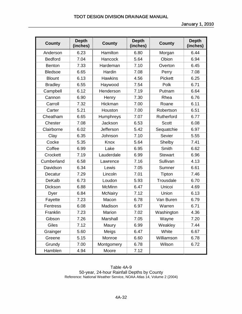
TDOT DESIGN DIVISION DRAINAGE MANUAL January 1, 2010
4A-32
County Depth (inches) County Depth
(inches) County Depth (inches)
Anderson 6.23 Hamilton 6.80 Morgan 6.44 Bedford 7.04 Hancock 5.64 Obion 6.94 Benton 7.33 Hardeman 7.10 Overton 6.45 Bledsoe 6.65 Hardin 7.08 Perry 7.08 Blount 6.13 Hawkins 4.56 Pickett 6.25
Bradley 6.55 Haywood 7.54 Polk 6.71 Campbell 6.12 Henderson 7.19 Putnam 6.64 Cannon 6.90 Henry 7.30 Rhea 6.76 Carroll 7.32 Hickman 7.00 Roane 6.11 Carter 5.21 Houston 7.00 Robertson 6.51
Cheatham 6.65 Humphreys 7.07 Rutherford 6.77 Chester 7.08 Jackson 6.53 Scott 6.08
Clairborne 6.02 Jefferson 5.42 Sequatchie 6.97 Clay 6.35 Johnson 7.10 Sevier 5.55
Cocke 5.35 Knox 5.64 Shelby 7.41 Coffee 6.99 Lake 6.95 Smith 6.62
Crockett 7.19 Lauderdale 6.99 Stewart 6.96 Cumberland 6.58 Lawrence 7.16 Sullivan 4.13
Davidson 6.34 Lewis 7.05 Sumner 6.61 Decatur 7.29 Lincoln 7.01 Tipton 7.46 DeKalb 6.73 Loudon 5.93 Trousdale 6.70 Dickson 6.88 McMinn 6.47 Unicoi 4.69
Dyer 6.84 McNairy 7.12 Union 6.13 Fayette 7.23 Macon 6.78 Van Buren 6.79
Fentress 6.08 Madison 6.97 Warren 6.71 Franklin 7.23 Marion 7.02 Washington 4.36 Gibson 7.26 Marshall 7.05 Wayne 7.20 Giles 7.12 Maury 6.99 Weakley 7.44
Grainger 5.60 Meigs 6.47 White 6.67 Greene 5.15 Monroe 6.60 Williamson 6.78 Grundy 7.00 Montgomery 6.78 Wilson 6.72
Hamblen 4.94 Moore 7.12
Table 4A-9 50-year, 24-hour Rainfall Depths by County
Reference: National Weather Service, NOAA Atlas 14, Volume 2 (2004)

TDOT DESIGN DIVISION DRAINAGE MANUAL January 1, 2010
4A-33
County Depth (inches) County Depth
(inches) County Depth (inches)
Anderson 6.97 Hamilton 7.52 Morgan 7.12 Bedford 7.78 Hancock 6.28 Obion 7.60 Benton 8.26 Hardeman 7.79 Overton 7.16 Bledsoe 7.35 Hardin 7.78 Perry 7.85 Blount 6.82 Hawkins 4.96 Pickett 6.95
Bradley 7.24 Haywood 8.48 Polk 7.46 Campbell 6.88 Henderson 8.11 Putnam 7.35 Cannon 7.63 Henry 8.23 Rhea 7.48 Carroll 8.26 Hickman 7.77 Roane 6.75 Carter 5.67 Houston 7.83 Robertson 7.25
Cheatham 7.42 Humphreys 7.89 Rutherford 7.50 Chester 7.88 Jackson 7.25 Scott 6.74
Clairborne 6.82 Jefferson 6.13 Sequatchie 7.72 Clay 7.07 Johnson 8.09 Sevier 6.28
Cocke 5.96 Knox 6.25 Shelby 8.26 Coffee 7.73 Lake 7.62 Smith 7.37
Crockett 7.99 Lauderdale 7.66 Stewart 7.78 Cumberland 7.27 Lawrence 7.92 Sullivan 4.46
Davidson 7.06 Lewis 7.79 Sumner 7.38 Decatur 8.17 Lincoln 7.74 Tipton 8.37 DeKalb 7.44 Loudon 6.56 Trousdale 7.48 Dickson 7.66 McMinn 7.15 Unicoi 5.09
Dyer 7.46 McNairy 7.81 Union 6.91 Fayette 7.99 Macon 7.59 Van Buren 7.51
Fentress 6.74 Madison 7.68 Warren 7.42 Franklin 8.01 Marion 7.77 Washington 4.72 Gibson 8.10 Marshall 7.79 Wayne 7.97 Giles 7.88 Maury 7.72 Weakley 8.37
Grainger 6.28 Meigs 7.15 White 7.37 Greene 5.72 Monroe 7.32 Williamson 7.54 Grundy 7.74 Montgomery 7.57 Wilson 7.48
Hamblen 5.45 Moore 7.88
Table 4A-10 100-year, 24-hour Rainfall Depths by County
Reference: National Weather Service, NOAA Atlas 14, Volume 2 (2004)

TDOT DESIGN DIVISION DRAINAGE MANUAL January 1, 2010
4A-34
Hydrologic Area
Watershed Area
Acres Square Miles
1 832 1.30 2 326 0.51 3 205 0.32 4 269 0.42
Table 4A-11 Drainage Area Required to Produce a 50-year Discharge
of 500 ft3/s or Greater Reference: TDOT Hydraulic Design Section

TDOT DESIGN DIVISION DRAINAGE MANUAL January 1, 2010
4A-35
4.06.2 EXAMPLE PROBLEMS 4.06.2.1 RATIONAL METHOD EXAMPLE PROBLEMS 4.06.2.1.1 SIMPLE DRAINAGE AREA DESIGN DISCHARGE EXAMPLE GIVEN: A ditch will collect runoff from the proposed roadway and an adjacent watershed. The tributary area has a fairly uniform cross section with 30 feet of bituminous concrete and shoulders, 15 feet of gravel lined ditch (1" stones), and 200 feet of meadow draining to the ditch. The ditch begins at a small summit and drains to a culvert for a length of 1,000 feet. The location of this proposed road is near Franklin, Tennessee.
Figure 4A-17
Simple Drainage Area Example FIND: The 50-year storm discharge to the culvert.

TDOT DESIGN DIVISION DRAINAGE MANUAL January 1, 2010
4A-36
Figure 4A-18 Ditch Cross Section for Simple Drainage Area Example
SOLUTION: Step 1: Determine the drainage area to verify that Rational Method is the proper method for analysis:
AREA = 1,000 ft x (30 ft + 15 ft + 200 ft) = 245,000 square feet = 5.62 acres
Since 5.62 acres is less than 100 acres and no other special conditions are identified, the Rational Method is selected (Q=CiA). Step 2: Determine the Runoff Coefficient:
Type of Surface AREA Runoff
Coefficient (C) (Table 4-2)
C x A Square Feet Acres
(A) Roadway (Bituminous Concrete) 30,000 0.69 0.9 0.62
Ditch (Gravel) 15,000 0.34 0.6 0.20 Meadow 200,000 4.59 0.3 1.38
TOTAL 245,000 5.62 2.20
Table 4A-12 Runoff Coefficient Calculation
Weighted C = 39.062.520.2
=

TDOT DESIGN DIVISION DRAINAGE MANUAL January 1, 2010
4A-37
Step 3: Find the Time of Concentration and Rainfall Intensity. Because the project is located in Franklin County, it falls within the Shelbyville IDF region as shown in Figure 4A-1. Thus, Figure 4A-11 will be used to determine rainfall intensity. The time of concentration for this drainage area includes overland flow travel time and channel travel time. The overland flow component is obtained from the Kinematic Wave equation or the NRCS TR-55 method because the flow is assumed to be sheet flow. Sheet flow is assumed because areas of shallow concentrated flow are not identified and the distance to the ditch is 200 feet, which is less than the 300 feet requirement where shallow concentrated flow would need to be considered.
A: Sheet Flow Travel Time:
Known parameters for Kinematic Wave equation: L = 200 feet n = 0.35 (Table 4-3 - assume "meadow" is similar to "pasture") S = 0.004 ft/ft C = 0.938 (constant for Kinematic Wave equation) Iteration 1
: Assume travel time, tt, for sheet flow = 10 minutes. Thus, from the IDF Curve, i50 = 7.75 in/hr. Then, using Equation (4-5),
3040
6060
..
..
t SiLnCt =
( ) ( )( ) ( )
7270040757
200350938010 3040
6060
...
..min ..
..
=→ min
Iteration 2
: Assume a higher sheet flow travel time, 35minutes. Thus, from the IDF Curve, i50 = 4.67 in./hr.
( ) ( )( ) ( )
0340040674
200350938035 3040
6060
...
..min ..
..
=→ min
Iteration 3
: Assume a lower sheet flow travel time, 33.8 minutes. Thus, from the IDF Curve, i50 = 4.73 in/hr
( ) ( )( ) ( )
8330040734
2003509380833 3040
6060
...
..min. ..
..
=→ min
Therefore, the travel time, tt, for sheet flow = 33.8 minutes.

TDOT DESIGN DIVISION DRAINAGE MANUAL January 1, 2010
4A-38
B. Channel Travel Time:
The channel flow velocity may be found using Equation (4-9). For this computation, a depth of 0.7 feet will be assumed.
Use Equation (4-9): 506704861 .c
.h S*R*
n.V =
Where: n = 0.084 (From Table 5A-10) A = 3.57 ft2 (Area) P = 7.43 ft (Wetted Perimeter) Rh = A/P = 0.48 Sc = 0.045 ft/ft (slope of channel). Thus:
32045048008404861 50670 .....V .. =××= fps
Next, find the channel travel time using Equation (4-3):
V
Lt )channel(t ×=
60= 27
32601000 .
.=
× min
C. Compute the Time of Concentration:
Use Equation (4-2): Tc = tt(sheet flow) + tt(channel) = 33.8 + 7.2 = 41.0 minutes
D. Rainfall Intensity:
From Figure 4A-11 where Tc = 41 minutes, i50 = 4.3 in/hr Step 4: Find the storm runoff rate: Use Equation (4-1): Q50 = CiA = (0.39) (4.3 in/hr) (5.62 acres) = 9.5 cfs Using the procedure provided in Section 5.06 for the design of vegetated ditches, the depth for this flow rate is found to be 0.94 feet which matches well with the depth assumed in the channel flow velocity computations shown above. In addition, this depth should be well below the subgrade of the roadway. Step 5: Check to see if the pavement alone provides higher discharge than the entire area including the meadow.
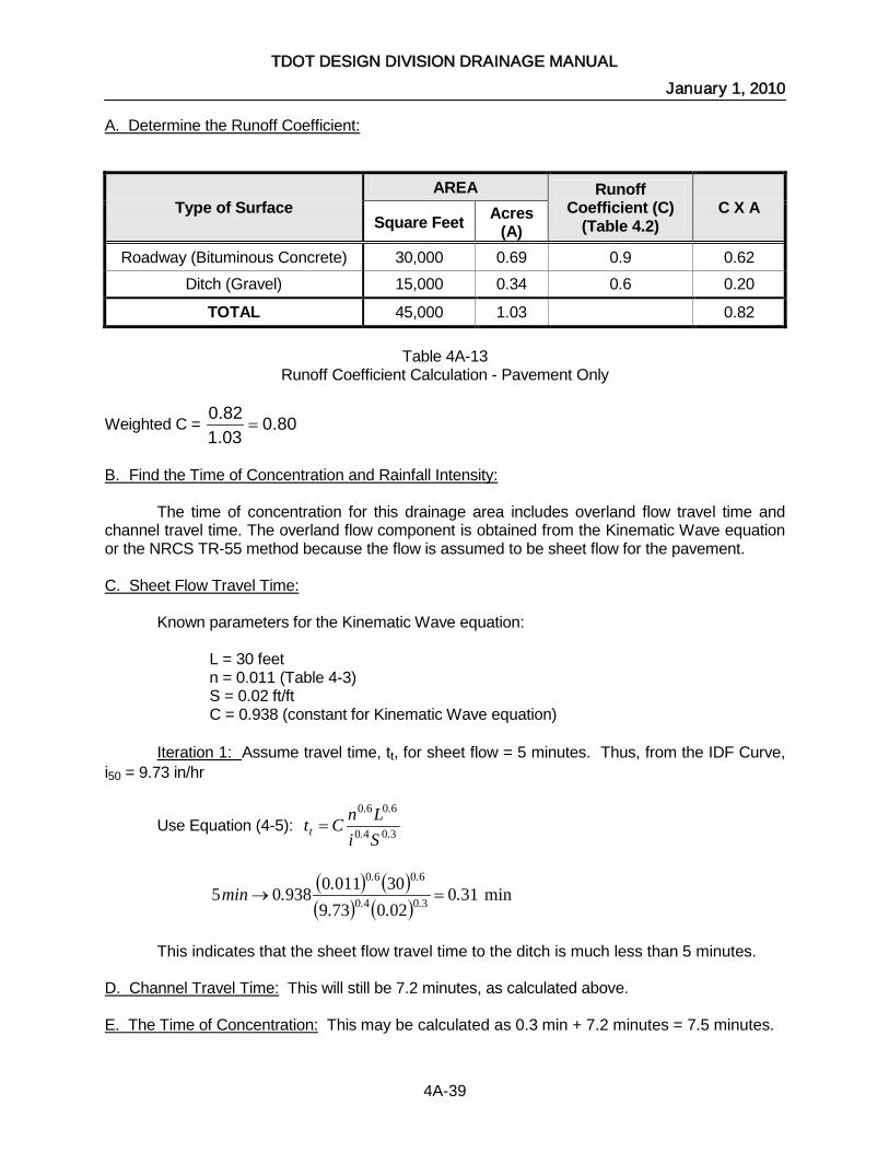
TDOT DESIGN DIVISION DRAINAGE MANUAL January 1, 2010
4A-39
A. Determine the Runoff Coefficient:
Type of Surface AREA Runoff
Coefficient (C) (Table 4.2)
C X A Square Feet Acres
(A) Roadway (Bituminous Concrete) 30,000 0.69 0.9 0.62
Ditch (Gravel) 15,000 0.34 0.6 0.20
TOTAL 45,000 1.03 0.82
Table 4A-13 Runoff Coefficient Calculation - Pavement Only
Weighted C = 80.003.182.0
=
B. Find the Time of Concentration and Rainfall Intensity:
The time of concentration for this drainage area includes overland flow travel time and channel travel time. The overland flow component is obtained from the Kinematic Wave equation or the NRCS TR-55 method because the flow is assumed to be sheet flow for the pavement.
C. Sheet Flow Travel Time:
Known parameters for the Kinematic Wave equation: L = 30 feet n = 0.011 (Table 4-3) S = 0.02 ft/ft C = 0.938 (constant for Kinematic Wave equation) Iteration 1:
Assume travel time, tt, for sheet flow = 5 minutes. Thus, from the IDF Curve, i50 = 9.73 in/hr
Use Equation (4-5): 3040
6060
..
..
t SiLnCt =
( ) ( )( ) ( )
31002073930011093805 3040
6060
...
..min ..
..
=→ min
This indicates that the sheet flow travel time to the ditch is much less than 5 minutes. D. Channel Travel Time:
This will still be 7.2 minutes, as calculated above.
E. The Time of Concentration: This may be calculated as 0.3 min + 7.2 minutes = 7.5 minutes.

TDOT DESIGN DIVISION DRAINAGE MANUAL January 1, 2010
4A-40
F. Rainfall Intensity
From Figure 4A-11 where Tc = 7.5 minutes, i50 = 8.7 in/hr
G. Find the Storm runoff rate:
Using Equation (4-1): Q50 = CiA = (0.80) (8.7 in/hr) (1.03 acres) = 7.2 cfs This indicates that the pavement and ditch provide a somewhat lower discharge than the entire drainage area. Step 6: Determine Design Discharge: The design discharge that should be used is 9.5 cfs because 9.5 cfs > 7.2 cfs.

TDOT DESIGN DIVISION DRAINAGE MANUAL January 1, 2010
4A-41
4.06.2.1.2 COMPLEX DRAINAGE AREA DESIGN DISCHARGE EXAMPLE GIVEN: A ditch will collect runoff from the proposed roadway and an adjacent watershed. The tributary area has a fairly uniform cross section with 30 feet of bituminous concrete and shoulders, 15 feet of grass lined ditch with some small shrubs and cattails, and 550 feet of forested land with light underbrush draining to the ditch. The ditch begins at a small summit and drains to a culvert for a length of 850 feet. The location of this proposed road is outside of Cleveland, Tennessee.
Figure 4A-19 Complex Drainage Area Example
Figure 4A-20 Ditch Cross Section for Complex Drainage Area Example
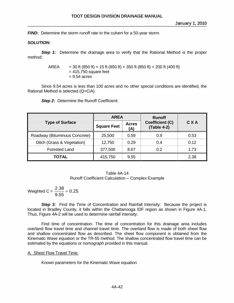
TDOT DESIGN DIVISION DRAINAGE MANUAL January 1, 2010
4A-42
FIND: Determine the storm runoff rate to the culvert for a 50-year storm. SOLUTION: Step 1: Determine the drainage area to verify that the Rational Method is the proper method:
AREA = 30 ft (850 ft) + 15 ft (850 ft) + 350 ft (850 ft) + 200 ft (400 ft) = 415,750 square feet = 9.54 acres
Since 9.54 acres is less than 100 acres and no other special conditions are identified, the Rational Method is selected (Q=CiA). Step 2: Determine the Runoff Coefficient:
Type of Surface AREA Runoff
Coefficient (C) (Table 4-2)
C X A Square Feet Acres
(A) Roadway (Bituminous Concrete) 25,500 0.59 0.9 0.53
Ditch (Grass & Vegetation) 12,750 0.29 0.4 0.12 Forested Land 377,500 8.67 0.2 1.73
TOTAL 415,750 9.55 2.38
Table 4A-14 Runoff Coefficient Calculation – Complex Example
Weighted C = 25.055.938.2
=
Step 3: Find the Time of Concentration and Rainfall Intensity: Because the project is located in Bradley County, it falls within the Chattanooga IDF region as shown in Figure 4A-1. Thus, Figure 4A-2 will be used to determine rainfall intensity. Find time of concentration. The time of concentration for this drainage area includes overland flow travel time and channel travel time. The overland flow is made of both sheet flow and shallow concentrated flow as described. The sheet flow component is obtained from the Kinematic Wave equation or the TR-55 method. The shallow concentrated flow travel time can be estimated by the equations or nomograph provided in this manual.
A. Sheet Flow Travel Time:
Known parameters for the Kinematic Wave equation

TDOT DESIGN DIVISION DRAINAGE MANUAL January 1, 2010
4A-43
L = 22 200400 + = 447 feet. (However, use 300 feet as this is the maximum allowed for sheet flow.) n = 0.400 (Table 4-3) S = 0.003 ft/ft C = 0.938 (constant for Kinematic Wave equation) Iteration 1: A
ssume travel time, tt, for sheet flow = 10 minutes. Thus, from the IDF Curve, i50 = 7.16 in/hr
Use Equation (4-5): 3040
6060
..
..
t SiLnCt =
( ) ( )( ) ( )
1430030167
300400938010 3040
6060
...
..min ..
..
=→ min
Iteration 2:
Assume a higher sheet flow travel time, 45 minutes. Thus, from the IDF Curve, i50 = 3.82 in/hr
( ) ( )( ) ( )
4550030823
300400938045 3040
6060
...
..min ..
..
=→ min
Iteration 3:
Assume a higher sheet flow travel time, 60 minutes. Thus, from the IDF Curve, i50 = 3.09 in/hr
( ) ( )( ) ( )
3600030093
300400938060 3040
6060
...
..min ..
..
=→ min
Iteration 4:
Assume a higher sheet flow travel time, 60.5 minutes. Thus, from the IDF Curve, i50 = 3.08 in/hr
( ) ( )( ) ( )
4600030083
300400938064 3040
6060
...
..min ..
..
=→ min
Therefore tt(sheet flow) = 60.4 minutes.
B. Shallow Concentrated Flow Travel Time:
First, find the Shallow Concentrated Flow velocity, using Equation (4-7): ( ) 50134516 .
unpaved S.V = Where S = 0.01 ft/ft. Thus,
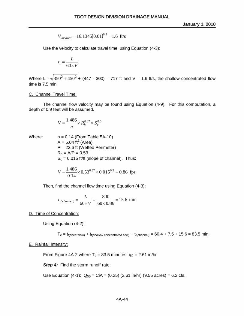
TDOT DESIGN DIVISION DRAINAGE MANUAL January 1, 2010
4A-44
( ) 61010134516 50 ...V .unpaved == ft/s
Use the velocity to calculate travel time, using Equation (4-3):
V
Ltt ×=
60
Where L = 22 450350 + + (447 - 300) = 717 ft and V = 1.6 ft/s, the shallow concentrated flow time is 7.5 min
C. Channel Travel Time:
The channel flow velocity may be found using Equation (4-9). For this computation, a depth of 0.9 feet will be assumed.
506704861 .c
.h SR
n.V ××=
Where: n = 0.14 (From Table 5A-10) A = 5.04 ft2 (Area) P = 22.6 ft (Wetted Perimeter) Rh = A/P = 0.53 Sc = 0.015 ft/ft (slope of channel). Thus:
8600150530140
4861 50670 ....
.V .. =××= fps
Then, find the channel flow time using Equation (4-3):
V
Lt )channel(t ×=
60= 615
86060800 .
.=
× min
D. Time of Concentration:
Using Equation (4-2): Tc = tt(sheet flow) + tt(shallow concentrated flow) + tt(channel) = 60.4 + 7.5 + 15.6 = 83.5 min.
E. Rainfall Intensity:
From Figure 4A-2 where Tc = 83.5 minutes, i50 = 2.61 in/hr Step 4: Find the storm runoff rate: Use Equation (4-1): Q50 = CiA = (0.25) (2.61 in/hr) (9.55 acres) = 6.2 cfs.

TDOT DESIGN DIVISION DRAINAGE MANUAL January 1, 2010
4A-45
Using the procedure provided in Section 5.06 for the design of vegetated ditches, the depth for this flow rate is found to be 0.94 feet which matches well with the depth assumed in the channel flow velocity computations shown above. In addition, this depth should be well below the subgrade of the roadway. Step 5: Check to see if the pavement alone provides higher discharge than forested area.
A. Determine the Runoff Coefficient:
Type of Surface AREA Runoff
Coefficient (C) (Table 4-2)
C X A Square Feet Acres
(A) Roadway (Bituminous Concrete) 25,500 0.59 0.9 0.53
Ditch (Gravel) 12,750 0.29 0.4 0.12
TOTAL 38,250 0.88 0.65
Table 4A-15 Runoff Coefficient Calculation – Complex Example Check
Weighted C = 73.088.065.0
=
B. Find Time of Concentration and Rainfall Intensity:
The time of concentration for this drainage area includes overland flow travel time and channel travel time. The overland flow component is obtained from the Kinematic Wave equation or the TR-55 method because the flow is assumed to be sheet flow for the pavement.
C. Sheet Flow Travel Time:
Known parameters for the Kinematic Wave equation. L = 30 feet n = 0.011 (Table 4-3) S = 0.015 ft/ft C = 0.938 (constant for Kinematic Wave equation) Iteration 1:
Assume that the sheet flow travel time, tt, will be 5 minutes. Thus, from the IDF Curve (Figure 4A-2), i50 = 9.0 in/hr
Use Equation (4-5): 3040
6060
..
..
t SiLnCt =
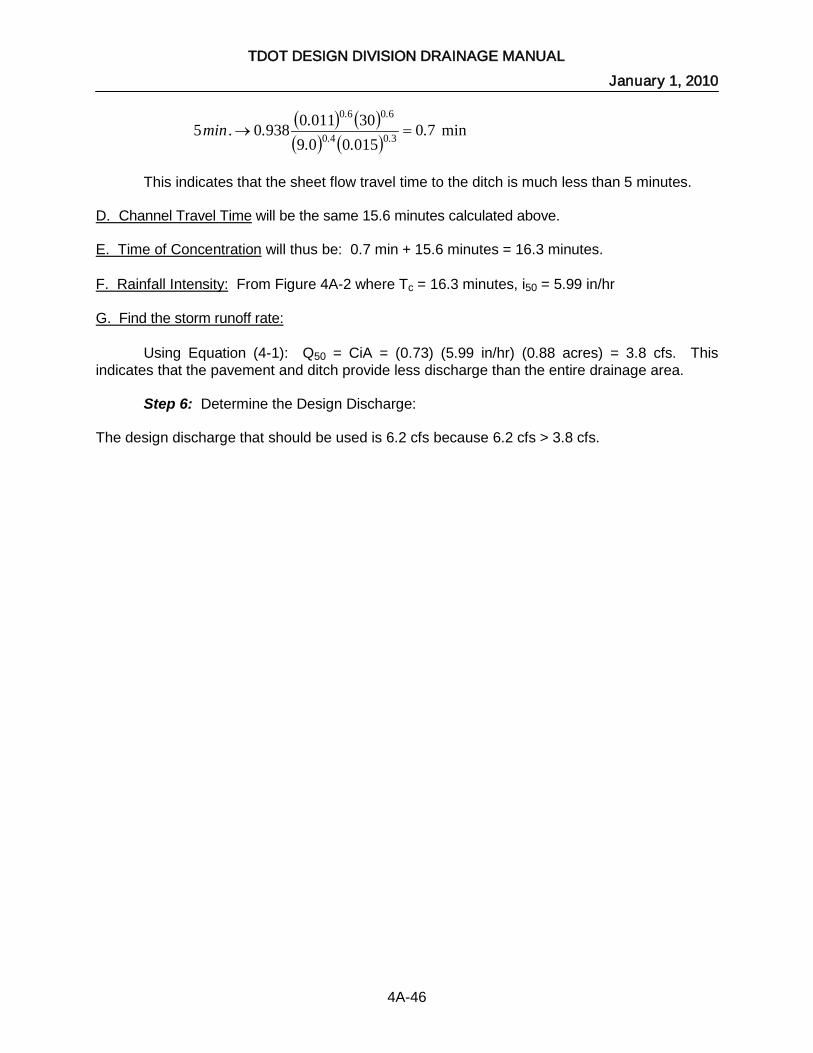
TDOT DESIGN DIVISION DRAINAGE MANUAL January 1, 2010
4A-46
( ) ( )( ) ( )
7001500930011093805 3040
6060
...
...min ..
..
=→ min
This indicates that the sheet flow travel time to the ditch is much less than 5 minutes. D. Channel Travel Time
will be the same 15.6 minutes calculated above.
E. Time of Concentration
will thus be: 0.7 min + 15.6 minutes = 16.3 minutes.
F. Rainfall Intensity:
From Figure 4A-2 where Tc = 16.3 minutes, i50 = 5.99 in/hr
G. Find the storm runoff rate:
Using Equation (4-1): Q50 = CiA = (0.73) (5.99 in/hr) (0.88 acres) = 3.8 cfs. This indicates that the pavement and ditch provide less discharge than the entire drainage area. Step 6: Determine the Design Discharge: The design discharge that should be used is 6.2 cfs because 6.2 cfs > 3.8 cfs.

TDOT DESIGN DIVISION DRAINAGE MANUAL January 1, 2010
4A-47
4.06.2.1.3 COMPUTER APPLICATION
Please refer to the current version of the GEOPAK Drainage program and associated documentation for flow analysis using the rational method.

TDOT DESIGN DIVISION DRAINAGE MANUAL January 1, 2010
4A-48
4.06.2.2 REGRESSION EQUATION EXAMPLES 4.06.2.2.1 RURAL REGRESSION EXAMPLE GIVEN: A drainage culvert located under SR-6 (U.S. 43) over a tributary to Bluewater Creek near Leoma, TN, Lawrence County. There was a USGS stream gaging station near this site from 1955 to 1983. The drainage area at the gage was 0.49 square miles (314 acres). FIND: The design flow for a culvert under this arterial route. SOLUTION: Step 1: Delineate and measure drainage area on USGS topographic quadrangles. Based on Figure 4A-21, the drainage area is 302 acres. Step 2: Determine in which Hydrologic Area the drainage basin is located in. Using Figure 4-3, the drainage area is found to be in Hydrologic Area 2. Step 3: Determine the design frequency and which regression equation to use. Table 4-1 indicates that the design frequency for a culvert under an arterial route is the 50-year storm. The equation to use for drainage areas greater 300 acres in Hydrologic Area 2 is in Table 4-4. Step 4: Compute 50-year recurrence interval design flow using the USGS Rural Regression Equation for Hydrologic Area 2. ( ) 7070
50 677 .CDAQ =
Where: CDA=302 acres. Thus, ( ) 398640302677 7070
50 == .Q ft3/s (Equation from Table 4-4). See Figures 4A-22a, 4A-22b and 4A-23 for the National Flood Frequency Program (NFF) inputs and outputs.

TDOT DESIGN DIVISION DRAINAGE MANUAL January 1, 2010
4A-49
Figure 4A-21
Bluewater Creek Tributary Drainage Area at SR-6

TDOT DESIGN DIVISION DRAINAGE MANUAL January 1, 2010
4A-50
Figure 4A-22a NFF Input Screen for Tennessee Rural Regression Equations
Figure 4A-22b NFF Output Screen for Tennessee Rural Regression Equations

TDOT DESIGN DIVISION DRAINAGE MANUAL January 1, 2010
4A-51
National Flood Frequency Program Version 3.0 Based on Water-Resources Investigations Report 02-4168 Equations from database C:\Download\NFF Install\NFFv3.2_2004-12-14.mdb Updated by kries 9/22/2004 at 4:03:24 PM fixed decimal place in constant Equations for Tennessee developed using English units Site: Bluewater Creek Trib near Leoma, Lawrence Co., Tennessee User: Date: Monday, December 05, 2005 08:28 AM Rural Estimate: Rural 1 Basin Drainage Area: 0.47 mi2 1 Region Region: DAOnly_Area_2 Contributing_Drainage_Area = 0.47 mi2 Flood Peak Discharges, in cubic feet per second Recurrence Peak, Standard Equivalent Estimate Interval, yrs cfs Error, % Years ____________________ _____________ _____ ________ __________ Rural 1 2 118 32 3.1 5 199 30 4.7 10 257 31 5.9 25 336 33 7.2 50 398 36 7.8 100 462 38 8.3 500 620 44 8.7
Figure 4A-23 NFF Output Report for Tennessee Rural Regression Equations

TDOT DESIGN DIVISION DRAINAGE MANUAL January 1, 2010
4A-52
4.06.2.2.2 STATEWIDE URBAN REGRESSION EXAMPLE GIVEN: A drainage culvert on Bybee Branch in McMinnville, TN, in Warren County. FIND: The design flow for the culvert under this collector route. SOLUTION: Step 1: Delineate and measure drainage area on USGS topographic quadrangle. Based on Figure 4A-24, the drainage area is 199 acres. Step 2: Determine the 2-year, 24-hour rainfall amount. Based on Table 4A-5, the 2-year, 24-hour rainfall is 3.71 inches. Step 3: The amount of impervious area in the watershed is estimated to be 30 acres or 15% of the watershed. Step 4: According to Table 4-1, the design frequency for a collector route is 50 years. Step 5: Compute the 50-year recurrence interval design flow rate. Since the project site is in an urban area, Equation 4-15 should be used. ( ) 421
242400750
50 640944 ..IMP
. PIA.Q −= Where: A = 199 acres IIMP = 15 percent P 2-24 = 3.71 inches. Thus, ( ) ( )( ) 35571315640199944 421400750
50 == ... ..Q ft3/s See Figures 4A-25a, 4A-25b and 4A-26 for the NFF inputs and outputs.

TDOT DESIGN DIVISION DRAINAGE MANUAL January 1, 2010
4A-53
Figure 4A-24 Bybee Branch Drainage Area

TDOT DESIGN DIVISION DRAINAGE MANUAL January 1, 2010
4A-54
Figure 4A-25a NFF Input Screen for Tennessee Statewide Urban Regression Equations
Figure 4A-25b NFF Output Screen for Tennessee Statewide Urban Regression Equations
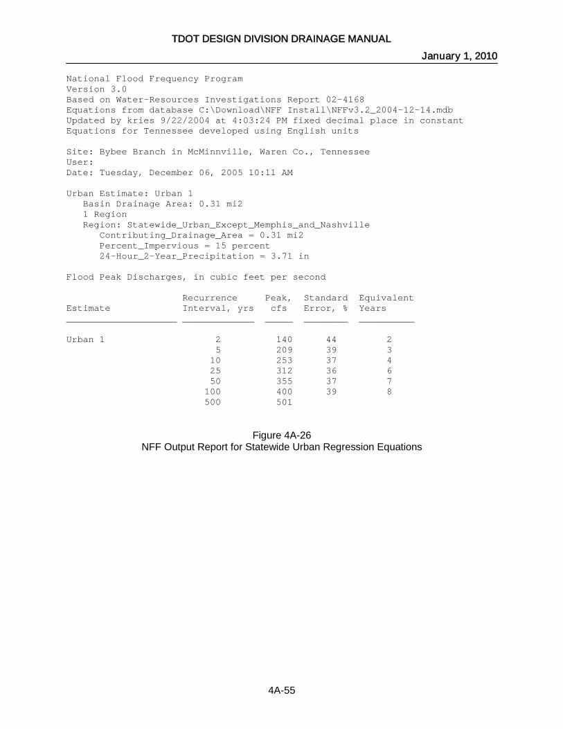
TDOT DESIGN DIVISION DRAINAGE MANUAL January 1, 2010
4A-55
National Flood Frequency Program Version 3.0 Based on Water-Resources Investigations Report 02-4168 Equations from database C:\Download\NFF Install\NFFv3.2_2004-12-14.mdb Updated by kries 9/22/2004 at 4:03:24 PM fixed decimal place in constant Equations for Tennessee developed using English units Site: Bybee Branch in McMinnville, Waren Co., Tennessee User: Date: Tuesday, December 06, 2005 10:11 AM Urban Estimate: Urban 1 Basin Drainage Area: 0.31 mi2 1 Region Region: Statewide_Urban_Except_Memphis_and_Nashville Contributing_Drainage_Area = 0.31 mi2 Percent_Impervious = 15 percent 24-Hour_2-Year_Precipitation = 3.71 in Flood Peak Discharges, in cubic feet per second Recurrence Peak, Standard Equivalent Estimate Interval, yrs cfs Error, % Years ____________________ _____________ _____ ________ __________ Urban 1 2 140 44 2 5 209 39 3 10 253 37 4 25 312 36 6 50 355 37 7 100 400 39 8 500 501
Figure 4A-26
NFF Output Report for Statewide Urban Regression Equations

TDOT DESIGN DIVISION DRAINAGE MANUAL January 1, 2010
4A-56
4.06.3 GLOSSARY The following list of terms is representative of those used in hydrologic analysis for drainage design. All of the terms may not necessarily be used in the chapter text; but rather are commonly used by engineers, scientists, and planners. ANTECEDENT MOISTURE CONIDTION (AMC)
– An index of moisture stored in the soils of a drainage area before a storm event occurs. This index accounts for the variation in curve number at a site due to recent previous rainfall events. Curve numbers presented in this Manual are based on AMC II, which represents average condition.
CHANNEL
– A long narrow depression associated with a waterway which is shaped by the concentrated flow of a stream and conveys the ordinary flows.
CHANNEL FLOW
– The flow of water in a defined conveyance such as a stream, ditch or pipe.
COUNTY SOIL SURVEYS
– Publications, usually produced by the NRCS, which provide detailed information on the properties of the soil types found in each county of the state. These surveys include aerial mapping which may be used to identify the soil types present on a specific site.
CURVE NUMBER
– A numeric parameter used to estimate the portion of the rainfall in a given precipitation event which will become runoff. The value of this parameter is based on a combination of the soil types present in a watershed and the land uses present on those soils (the soil-cover complex).
DESIGN FREQUENCY
– A selected storm event, described in terms of the probability of occurrence once within a given number of years, for which stormwater drainage facilities or other flood control improvements are designed. For example, a 5-year, 24-hour duration storm event has a 20 percent probability of occurring in any given year. The precipitation associated with that storm would be measured over a 24 hour period.
DETENTION
– The collection of stormwater runoff into a surface reservoir so that the water can be released at a reduced rate. Detention will typically be used to reduce the peak discharge from developed area to a rate that is equal to or less than the pre-developed condition (c.f. – Retention, Extended Detention).
DISCHARGE
– The quantity of flow, usually expressed as the number of cubic feet of water passing a given point in one second (ft3/s).
DRAINAGE AREA
– All of the area which will contribute runoff to a given point.
DURATION (of Rainfall)
– The length of time between the start of a given rainfall event and its finish.
EVAPORATION
– The part of the hydrologic cycle in which liquid water on the ground surface is converted to vapor and enters the atmosphere.
FLOOD INSURANCE STUDY – A document, usually published by the Federal Emergency Management Agency, which provides information on flood flow rates, flood elevations and the extent of floodplains within a given town, city or county.

TDOT DESIGN DIVISION DRAINAGE MANUAL January 1, 2010
4A-57
GUTTER
– A narrow channel usually at the edge of a roadway specifically used to collect and convey stormwater runoff. Normally placed with a curb.
HYDROGRAPH
– A graphic representation showing variation in discharge or depth (stage) of a stream of water over a specified period of time. May be defined in terms of discharge from a stormwater basin or runoff from a watershed.
HYDROLOGIC CONDITION
– An indication of the effects of cover type and treatment on infiltration rates. For example, good hydrologic condition indicates that the soil has a low runoff potential for its specific hydrologic soil group, cover type, and treatment.
HYDROLOGIC SOIL GROUP
– A classification of different soil types into groups (A, B, C, and D) according to their minimum infiltration rate, based upon bare soil after prolonged wetting.
HYDROLOGY
– The scientific study of the properties, distribution, and effects of water on the earth's surface, in the soil and underlying rocks, and in the atmosphere. As applied in engineering design, hydrology often refers to the determination of flood flow rates for the design of hydraulic structures such as cross drains or detention ponds.
IMPERVIOUS AREA
– The permanent surfaces in a drainage basin which cannot infiltrate rainfall. Areas typically consist of rooftops, sidewalks, pavements, slabs, driveways, etc.
INFILTRATION
– As applied in Hydrology, the process by which water percolates into soil and becomes a part of the groundwater regime. Water which infiltrates during a rainfall event is removed from the direct runoff and usually does not contribute to the peak flood flow rate a stream.
INITIAL ABSTRACTION
– In the curve number method, this is the quantity of rainfall, usually expressed as inches of depth, which must infiltrate into the soil before direct runoff can begin.
INTENSITY (of Rainfall)
– The rate at which rainfall occurs, usually expressed as inches of rainfall per hour (in/hr).
LOSS RATE
– The rate at which water from a rainfall event will infiltrate into the soil. Usually refers to infiltration which occurs once the initial abstraction has been satisfied.
N-VALUE
– An empirical number assigned to a given material as a gage of its frictional resistance to the flow of water.
OVERLAND FLOW
– Sheet flow beginning from the point at the top of watershed where runoff begins to the point at which flows begin to concentrate.
RATIONAL METHOD
– A means of determining flow rates for the design of drainage structures based upon the drainage area, rainfall intensity and runoff coefficient. (see Runoff Coefficient).
REGULATED STREAM
– A stream or other watercourse on which flows, especially flood flows, are affected by the presence of a man-made structure, usually a reservoir or detention pond.
ROUTING – The determination of the attenuating effect of storage on a storm passing though a stormwater management facility.

TDOT DESIGN DIVISION DRAINAGE MANUAL January 1, 2010
4A-58
RUNOFF
– The portion of the water from a rainfall event which flows across the surface of the ground.
RUNOFF COEFFICIENT
– A ratio, defined for a given soil type or land use, of the rate of direct runoff to the average rate of rainfall in a storm event.
SHALLOW CONCENTRATED FLOW
– An overland flow condition which occurs as sheet flows begin to collect into rills or other small low areas on the surface of the ground. This condition is intermediate between sheet flow and channel flow.
SHEET FLOW
– A flow condition in which water moves across the ground surface in a thin sheet. This is usually the first step in the process of forming runoff and can persist only for a short distance before water is concentrated into ground surface irregularities.
TIME OF CONCENTRATION
-- The time required for a particle of stormwater runoff to flow from the most hydrologically distant point in a drainage area to the point of interest, such as an inlet.
TRANSPIRATION
– The removal of moisture from the soil by terrestrial plants. This moisture is taken up by the roots and then evaporated into the atmosphere from the leaves.
TREATMENT (of Soil)
– A cover type modifier used in the determination of curve numbers for cultivated agricultural lands. It includes mechanical practices, such as contouring and terracing, and management practices, such as crop rotation and reduced or no tillage.
UNIT HYDROGRAPH
– The hydrograph which represents a runoff volume of 1 inch associated with a precipitation event of a specified duration. The unit hydrograph is a theoretical hydrograph which is intended to describe how a river at a particular point will react to one inch of runoff, and which can in turn be used to derive how the river will react to any amount of runoff.

TDOT DESIGN DIVISION DRAINAGE MANUAL January 1, 2010
4A-59
4.06.4 REFERENCES American Association of State Highway and Transportation Officials. Model Drainage Manual [Metric Edition]. Washington, D.C. 1999. American Society of Civil Engineers and Water Environment Federation. Design and Construction of Urban Stormwater Management Systems. ASCE Manuals and Reports of Engineering Practice No. 77 and WEF Manual of Practice FD-20. New York, New York and Alexandria, Virginia. 1992 Bonnin, Geoffrey M., et. al. NOAA Atlas 14, Precipitation-Frequency Atlas of the United States, Volume 2. United States Department of Commerce, National Oceanic and Atmospheric Administration, 2004. "Flood Frequency and Storm Runoff of Urban Areas of Memphis and Shelby County, Tennessee” Water-Resources Investigations Report 84-4110. United States Geological Survey. 1984. "Flood Frequency of Streams in Rural Basins of Tennessee" Water-Resources Investigations Report 92-4165. United States Geological Survey. 1993. “Flood Frequency Prediction Methods for Unregulated Streams of Tennessee” Water-Resources Investigations Report 03-4176. United States Geological Survey. 2003. Hankins, Jr., A.L. Guidelines for Drainage Studies and Hydraulic Design North Carolina Department of Transportation. Raleigh, NC. 1999. Illinois Department of Transportation Bureau of Bridges and Structures. Drainage Manual. August 1, 1989. Indiana Department of Transportation. Indiana Design Manual Part IV Volume I. Indianapolis, IN. 1999. Kentucky Transportation Cabinet, Drainage Guidance Manual - Proposed Revisions. Frankfort, KY. September 29, 2000. Lichty, R.W., and Liscum, F., 1978, A Rainfall-runoff Modeling Procedure for Improving Estimates of T-year (Annual) Floods for Small Drainage Basins. U.S. Geological Survey Water-Resources Investigations Report 78-7. Louisiana Department of Transportation and Development Hydraulics Section. Hydraulics Manual. March 1987. Metropolitan Government of Nashville and Davidson County Department of Public Works Engineering Division. Stormwater Management Manual. Nashville, Tennessee. Sept. 1999. Ragan, R. M., "A Nomograph Based on Kinematic Wave Theory for Determining Time of Concentration for Overland Flow," Report Number 44, Civil Engineering Department, University of Maryland at College Park, 1971.
TDO
T DESIG
N D
IVISION
DR
AIN
AG
E MA
NU
AL
February 1, 2005

TDOT DESIGN DIVISION DRAINAGE MANUAL January 1, 2010
4A-60
Schall, James D. and Richardson Everitt V. Introduction to Highway Hydraulics Hydraulic Design Series Number 4. Federal Highway Administration, April 1997 (available for download at www.fhwa.dot. gov./bridge/hydpub.htm
)
Searcy, James K, Design of Roadside Channels - HDS 4. U.S. Department of Transportation, Federal Highway Administration. May 1965 (available for download at www.fhwa.dot. gov./bridge/hydpub.htm
)
"Synthesized Flood Frequency for Small Urban Streams in Tennessee" Water-Resources Investigations Report 84-4182. United States Geological Survey. 1984. Tennessee Department of Transportation. Design Guidelines - English. Nashville, TN. 2001. United States Department of Agriculture. Soil Conservation Service. Engineering Division. Urban Hydrology for Small Watersheds - Technical Release 55. June 1986. (The software and manual are available at http://www.wcc.nrcs.usda.gov/water/quality/common/tr55/tr55.html). United States Department of Agriculture Soil Conservation Service, 1992, Computer Program for Project Formulation – Hydrology Users Manual. Technical Release No. 20. (The software and manual are available at http://www.wcc.nrcs.usda.gov/water/quality/wst.html). United States Department of Commerce. National Oceanic and Atmospheric Administration. National Weather Service. “Precipitation Frequency Data Server.” November, 21, 2005. http://hdsc.nws.noaa.gov/hdsc/pfds United States Department of Commerce, 1961, Rainfall Frequency Atlas of the United States for Durations from 30 minutes to 24 hours and Return Periods from 1 to 100 years, U.S. Weather Bureau Technical Paper No. 40. United States Department of Commerce, 1977, Five to 60-minutes Precipitation Frequency for Eastern and Central United States, U.S. National Weather Service Technical Memorandum No. 35. United States Army Corps of Engineers, 1998, HEC-1 Flood Hydrograph Package – Users Manual Version 4.1, Hydrologic Engineering Center. (The software and manuals are available at http://www.hec.usace.army.mil/software_distrib/index.html ) United States Army Corps of Engineers, 2001, Hydrologic Modeling System HEC-HMS Users Manual Version 2.1, Hydrologic Engineering Center. (The software and manuals are available at http://www.hec.usace.army.mil/software_distrib/index.html ) United States Geological Survey. “Water Resources Application Software, NFF, Version 3.2” September 9, 2005 http://water.usgs.gov/software/nff.html Virginia Department of Transportation. Drainage Manual. Richmond, Virginia. February 1989.

TDOT DESIGN DIVISION DRAINAGE MANUAL January 1, 2010
4A-61
4.06.5 ABBREVIATIONS AASHTO – American Association of State Highway Transportation Officials BLM – Bureau of Land Management CFR – Code of Federal Regulations CFS – Cubic feet per second COE – U.S. Army Corps of Engineers EOC – Emergency Operation Center EPA – U.S. Environment Protection Agency FBFM – Flood Boundary and Floodway Map FEMA – Federal Emergency Management Agency FHBM – Flood Hazard Boundary Map FHWA – Federal Highway Administration FIRM – Flood Insurance Rate Map FIS – Flood Insurance Studies FWS – United States Fish and Wildlife Service HDS-4 – Introduction to Highway Hydraulics Hydraulic Design Series Number 4 HEC-1 – Hydrologic Engineering Center Flood Hydrograph Package HEC-HMS – Hydrologic Engineering Center Hydrologic Modeling System HSG – Hydrologic Soil Group IDF – Intensity Duration Frequency ISTEA – 1991 Intermodal Surface Transportation Efficiency Act NFF – National Flood Frequency NFIP – National Flood Insurance Program NOAA – National Oceanic and Atmospheric Administration NRCS – Natural Resources Conservation Service (formerly Soil Conservation Service) NWS – National Weather Service SCS – Soil conservation Service TR-20 – The Natural Resources Conservation Service Technical Release 20 TR-55 – Urban Hydrology for Small Watersheds- Technical Release 55 USFS – U.S. Forest Service USGS – United States Department of the Interior, Geological Survey USWB – United States Department of Commerce, Weather Bureau WS – Water Surface