Taxonomic and regional uncertainty in species-arearelationships and the identification ofrichness hotspotsFrancois Guilhaumon*†, Olivier Gimenez‡, Kevin J. Gaston§, and David Mouillot*

*Laboratoire Ecosystemes Lagunaires, Unite Mixte de Recherche 5119, Centre National de la Recherche Scientifique-IFREMER-UM2, Universite Montpellier 2,cc 093, Place Eugene Bataillon, 34095 Montpellier Cedex 5, France; ‡Centre d’Ecologie Fonctionnelle et Evolutive, Unite Mixte de Recherche 5175, CentreNational de la Recherche Scientifique, 1919 Route de Mende, F-34293 Montpellier Cedex 5, France; and §Biodiversity and Macroecology Group, Departmentof Animal and Plant Sciences, University of Sheffield, Sheffield S10 2TN, United Kingdom

Edited by Michael P. H. Stumpf, Imperial College London, London, United Kingdom, and accepted by the Editorial Board August 22, 2008(received for review April 14, 2008)

Species-area relationships (SARs) are fundamental to the study ofkey and high-profile issues in conservation biology and are par-ticularly widely used in establishing the broad patterns of biodi-versity that underpin approaches to determining priority areas forbiological conservation. Classically, the SAR has been argued ingeneral to conform to a power-law relationship, and this form hasbeen widely assumed in most applications in the field of conser-vation biology. Here, using nonlinear regressions within an infor-mation theoretical model selection framework, we included un-certainty regarding both model selection and parameterestimation in SAR modeling and conducted a global-scale analysisof the form of SARs for vascular plants and major vertebrategroups across 792 terrestrial ecoregions representing almost 97%of Earth’s inhabited land. The results revealed a high level ofuncertainty in model selection across biomes and taxa, and that thepower-law model is clearly the most appropriate in only a minorityof cases. Incorporating this uncertainty into a hotspots analysisusing multimodel SARs led to the identification of a dramaticallydifferent set of global richness hotspots than when the power-lawSAR was assumed. Our findings suggest that the results of analysesthat assume a power-law model may be at severe odds with realecological patterns, raising significant concerns for conservationpriority-setting schemes and biogeographical studies.

conservation biology � ecoregions � model selection � vascular plants �vertebrates

Species-area relationships (SARs), the change in speciesnumbers with increasing area, are fundamental to the

present understanding of many key and high-profile issues inconservation biology. They have, for example, variously beenused to predict regional species extinction rates after habitat loss,as a consequence of such pressures as deforestation and climatechange (1–4) and to predict species extinction rates in blocks ofremnant habitat, including protected areas, as a consequence oftheir isolation (5). More fundamentally, the SAR is an essentialtool used to estimate broad patterns and to identify hotspots ofspecies richness when regions differ in area (6–13).

In the main, applications of SARs have assumed that theserelationships take the classical form of a log-linearizable powerfunction, S � cAz, where S is species richness, A is area, and c andz are constants (14). Depending on the objectives and opportu-nities, the parameters of this function (notably the exponent, orrate, z) are derived from theory (15–18), from particular datasetsor from broad collations of datasets (19–22). However, althoughthe power function has been applied extremely widely, in prac-tice there is much variation in the basic form of SARs (23, 24).Attention has focused foremost on how this form changes withspatial scale (25–27) or assemblage properties (28). Other kindsof systematic variation may also exist, but analyses have princi-pally only rather narrowly addressed these by comparing the

parameter values estimated from fitting a power function rela-tionship (e.g., space, refs. 21, 29, 30; environment, ref. 31; andanthropogenic threats, ref. 22).

Given that a single generic form for SARs is widely assumedto pertain, of particular concern for conservation biology wouldbe if the underlying form actually differed markedly betweenmajor taxonomic groups and/or biomes (global-scale biogeo-graphic regions distinguished by unique collections of ecosys-tems and species assemblages; ref. 32). Whether such variationwas systematic, it could have significant implications particularlyfor the fundamental understanding of the distribution of biodi-versity that underlies much of the prioritization of lands forconservation investment and action (33). For example, studieshave variously sought to incorporate the effects of variation inarea on species richness at large spatial scales (often ecoregions)when considering the concordance of spatial variation in richnessof different higher taxa (13, 34), patterns of protected areacoverage (35), the impacts of urbanization on biodiversity (36),and the allocation of conservation resources (37, 38).

In this article, we conduct an analysis of global-scale SARswith two aims. First, we investigate the uncertainty about thebest-fitting SAR model by quantifying the relative probabilitiesthat different models best describe SARs and determine whetherthose probabilities vary systematically for the same higher taxonin different biomes and for different higher taxa in the samebiome. Second, we conduct a global identification of hotspots ofrichness, incorporating the uncertainty about the best-fit SARmodel, and compare these results with those obtained when it isassumed that the power model is the best-fitting SAR model. Weuse data on the species richness of vascular plants and verte-brates across the world’s terrestrial ecoregions (13, 39) [support-ing information (SI) Text and Table S1]. Ecoregions are largeunits of land containing geographically distinct species assem-blages and experiencing geographically distinct environmentalconditions and have proven valuable for addressing a range ofissues in conservation prioritization (13, 40, 41).

ResultsTaxonomic and Regional Uncertainty in Species-Area Relationships.The relative fit of eight different potential forms for SARs(Table S2) was evaluated for each combination of higher taxon

Author contributions: F.G., O.G., K.J.G., and D.M. designed research; F.G., O.G., K.J.G., andD.M. performed research; F.G., O.G., K.J.G., and D.M. analyzed data; and F.G., O.G., K.J.G.,and D.M. wrote the paper.

The authors declare no conflict of interest.

This article is a PNAS Direct Submission. M.P.H.S. is a guest editor invited by the EditorialBoard.

†To whom correspondence should be addressed. E-mail: francois.guilhaumon@univ-montp2.fr.

This article contains supporting information online at www.pnas.org/cgi/content/full/0803610105/DCSupplemental.

© 2008 by The National Academy of Sciences of the USA

15458–15463 � PNAS � October 7, 2008 � vol. 105 � no. 40 www.pnas.org�cgi�doi�10.1073�pnas.0803610105

Dow

nloa

ded

by g

uest

on

Dec

embe

r 23

, 201

9

and biome. These forms encompassed convex, sigmoid, asymp-totic, and nonasymptotic models, with the fit being evaluatedusing nonlinear regressions in the so-called model selectionframework (42). This emerging approach in the context of SARs(43) aims to evaluate, for a given dataset, the strength ofevidence for alternative explanatory models (44). Furthermore,by averaging across statistically valid models, this frameworkallows the construction of robust inferences incorporating un-certainty regarding both model selection and parameter estima-tion (multimodel SARs; see Materials and Methods for details).

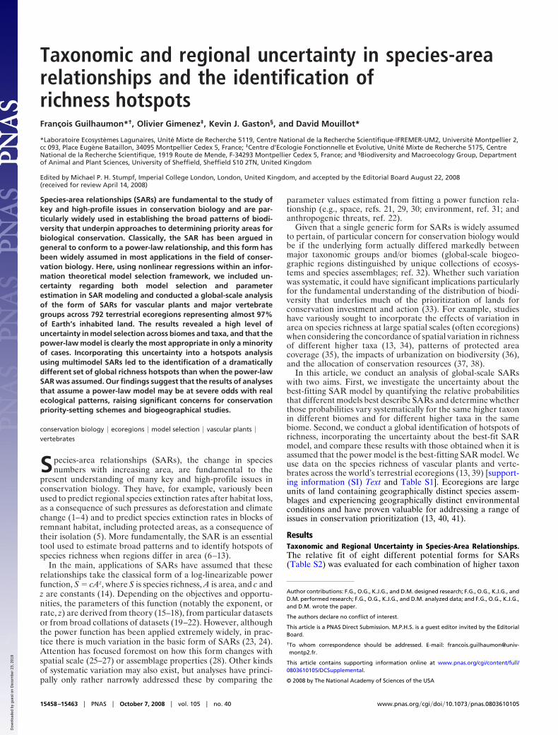
Surprisingly, given the apparent generality of the SAR, theanalysis revealed substantial variation in the strength of theeffect of area on species richness. Although the R2 for multi-model SARs had an overall mean of 0.30, values for differentcombinations of higher taxa and biomes ranged from 0.02 foramphibians in Tropical Dry Forests to 0.69 for total vertebratesin Tropical Grasslands (Table S3). Furthermore, for severaldatasets (21 of 78), the SAR cannot be adequately described byany of the candidate models (Fig. 1, Table S4). This lattertendency was not limited to those datasets with narrower rangesof variation in species richness or area but is more obvious forbiomes than for higher taxa. For example, SARs were statisti-cally validated across temperate forest ecoregions only formammals and vascular plants.

The best-fitting model varied markedly across biomes for allhigher taxa and across higher taxa for each biome (Fig. 1, TableS4). It was the asymptotic negative exponential (convex) and theMonod (convex) models in 18 and 13 cases, respectively, thenonasymptotic power and exponential models in 10 cases each,and the logistic and Lomolino models in five and one case,respectively. The rational function and the cumulative Weibullmodels never provided the best fit. However, with the exceptionof four datasets (amphibians and mammals in Tropical andSubtropical Moist Broadleaf Forests, vascular plants in Temper-ate Conifer Forests, and reptiles in Deserts), there was asubstantial degree of uncertainty about the best-fitting SARmodel (Fig. 1, Table S4). For most of the datasets, no singlemodel was clearly superior.

Furthermore, for almost all higher taxa, model probabilitiesdiffered markedly across biomes (Fig. 1, Table S4). Although foralmost all biomes, model probabilities also differed markedlyacross higher taxa (Fig. 1, Table S4), summing these probabilitiesacross the different models revealed some coarse tendencies.Indeed, for Boreal Forests, except for amphibians, the sum of theprobabilities of nonasymptotic models that best describe theSAR was always �0.5. In contrast, for the Tundra and Medi-terranean Forests, the SAR was likely to be asymptotic for mosthigher taxa (Fig. 1, Table S4).

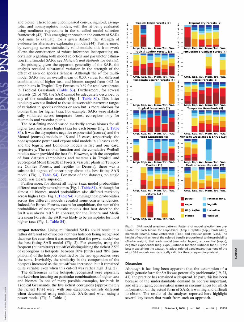
Hotspot Detection. Using multimodel SARs could result in arather different set of species richness hotspots being recognizedthan was the case when it was assumed that the power model wasthe best-fitting SAR model (Fig. 2). For example, using thefrequent (but arbitrary) cut-off of distinguishing the richest 2.5%of ecoregions as hotspots, between 30% (birds) and 78% (am-phibians) of the hotspots identified by the two approaches werethe same. Inevitably, the similarity in the composition of thehotspots increased as the cut-off was increased, but it remainedquite variable even when this cut-off was rather high (Fig. 2).

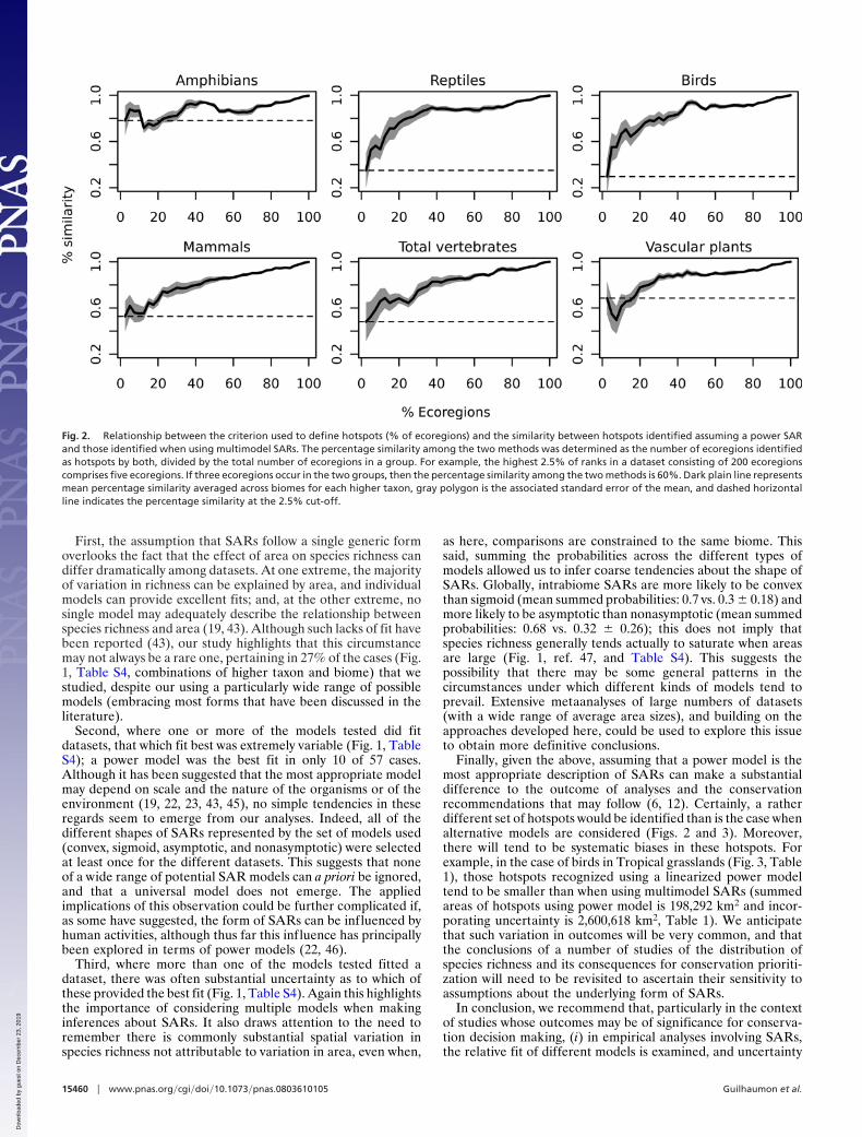
The differences in the hotspots recognized were especiallymarked when focusing on particular combinations of higher taxaand biomes. In one of many possible examples, for birds inTropical Grasslands, the five richest ecoregions (approximatelythe richest 10%) were, with one exception, entirely differentwhen determined using multimodel SARs and when using apower model (Fig. 3, Table 1).

DiscussionAlthough it has long been apparent that the assumption of asingle generic form for SARs was potentially problematic (19, 23,43), the practice has remained widespread. In part, this has beenbecause of the understandable demand to address important,and often urgent, conservation issues in circumstances for whichinformation on the actual form of SARs is wanting and difficultto obtain. The results of the analyses reported here highlightseveral key issues that result from such an approach.

Fig. 1. SAR model selection patterns. Patterns of model selection are pre-sented for each biome for amphibians (Amp.), reptiles (Rep.), birds (Avi.),mammals (Mam.), total vertebrates (Tot.), and vascular plants (Vas.). Theheight of each fraction of the colored band is proportional to the probability(Akaike weight) that each model [see color legend, exponential (expo.),negative exponential (neg. expo.), rational function (rational func.)] is thebest in explaining the dataset. A lack of colored band means that none of theeight SAR models was statistically valid for the corresponding dataset.

Guilhaumon et al. PNAS � October 7, 2008 � vol. 105 � no. 40 � 15459

ECO

LOG

Y

Dow

nloa

ded

by g

uest

on

Dec

embe

r 23

, 201

9

First, the assumption that SARs follow a single generic formoverlooks the fact that the effect of area on species richness candiffer dramatically among datasets. At one extreme, the majorityof variation in richness can be explained by area, and individualmodels can provide excellent fits; and, at the other extreme, nosingle model may adequately describe the relationship betweenspecies richness and area (19, 43). Although such lacks of fit havebeen reported (43), our study highlights that this circumstancemay not always be a rare one, pertaining in 27% of the cases (Fig.1, Table S4, combinations of higher taxon and biome) that westudied, despite our using a particularly wide range of possiblemodels (embracing most forms that have been discussed in theliterature).

Second, where one or more of the models tested did fitdatasets, that which fit best was extremely variable (Fig. 1, TableS4); a power model was the best fit in only 10 of 57 cases.Although it has been suggested that the most appropriate modelmay depend on scale and the nature of the organisms or of theenvironment (19, 22, 23, 43, 45), no simple tendencies in theseregards seem to emerge from our analyses. Indeed, all of thedifferent shapes of SARs represented by the set of models used(convex, sigmoid, asymptotic, and nonasymptotic) were selectedat least once for the different datasets. This suggests that noneof a wide range of potential SAR models can a priori be ignored,and that a universal model does not emerge. The appliedimplications of this observation could be further complicated if,as some have suggested, the form of SARs can be influenced byhuman activities, although thus far this influence has principallybeen explored in terms of power models (22, 46).

Third, where more than one of the models tested fitted adataset, there was often substantial uncertainty as to which ofthese provided the best fit (Fig. 1, Table S4). Again this highlightsthe importance of considering multiple models when makinginferences about SARs. It also draws attention to the need toremember there is commonly substantial spatial variation inspecies richness not attributable to variation in area, even when,

as here, comparisons are constrained to the same biome. Thissaid, summing the probabilities across the different types ofmodels allowed us to infer coarse tendencies about the shape ofSARs. Globally, intrabiome SARs are more likely to be convexthan sigmoid (mean summed probabilities: 0.7 vs. 0.3 � 0.18) andmore likely to be asymptotic than nonasymptotic (mean summedprobabilities: 0.68 vs. 0.32 � 0.26); this does not imply thatspecies richness generally tends actually to saturate when areasare large (Fig. 1, ref. 47, and Table S4). This suggests thepossibility that there may be some general patterns in thecircumstances under which different kinds of models tend toprevail. Extensive metaanalyses of large numbers of datasets(with a wide range of average area sizes), and building on theapproaches developed here, could be used to explore this issueto obtain more definitive conclusions.

Finally, given the above, assuming that a power model is themost appropriate description of SARs can make a substantialdifference to the outcome of analyses and the conservationrecommendations that may follow (6, 12). Certainly, a ratherdifferent set of hotspots would be identified than is the case whenalternative models are considered (Figs. 2 and 3). Moreover,there will tend to be systematic biases in these hotspots. Forexample, in the case of birds in Tropical grasslands (Fig. 3, Table1), those hotspots recognized using a linearized power modeltend to be smaller than when using multimodel SARs (summedareas of hotspots using power model is 198,292 km2 and incor-porating uncertainty is 2,600,618 km2, Table 1). We anticipatethat such variation in outcomes will be very common, and thatthe conclusions of a number of studies of the distribution ofspecies richness and its consequences for conservation prioriti-zation will need to be revisited to ascertain their sensitivity toassumptions about the underlying form of SARs.

In conclusion, we recommend that, particularly in the contextof studies whose outcomes may be of significance for conserva-tion decision making, (i) in empirical analyses involving SARs,the relative fit of different models is examined, and uncertainty

Fig. 2. Relationship between the criterion used to define hotspots (% of ecoregions) and the similarity between hotspots identified assuming a power SARand those identified when using multimodel SARs. The percentage similarity among the two methods was determined as the number of ecoregions identifiedas hotspots by both, divided by the total number of ecoregions in a group. For example, the highest 2.5% of ranks in a dataset consisting of 200 ecoregionscomprises five ecoregions. If three ecoregions occur in the two groups, then the percentage similarity among the two methods is 60%. Dark plain line representsmean percentage similarity averaged across biomes for each higher taxon, gray polygon is the associated standard error of the mean, and dashed horizontalline indicates the percentage similarity at the 2.5% cut-off.

15460 � www.pnas.org�cgi�doi�10.1073�pnas.0803610105 Guilhaumon et al.

Dow

nloa

ded

by g

uest

on

Dec

embe

r 23

, 201

9

in this fit is accounted for; and (ii) in more theoretical studiesinvolving SARs, the consequences of assuming different under-lying forms of these relationships are examined. Failing to do somay well lead to conclusions at odds with real patterns of spatialvariation in species richness, as exemplified in the identificationof hotspots of richness among areas of differing size.

Materials and MethodsData. Analyses were based on the numbers of species of vascular plants,amphibians, reptiles, birds, and mammals in each terrestrial ecoregion of the

world as delimited by Olson et al. (32). Data were obtained on vertebrates byoverlaying range maps of extant species compiled from numerous scientificworks, field guides, or directly from experts (32), and on vascular plants frompublished and unpublished richness data and from a variety of additionalinformation (39). Following Lamoreux et al. (13), we excluded Mangroveecoregions and large uninhabited parts of Greenland and Antarctica becauseof lack of data reliability or availability. The resulting database contains 78datasets (combinations across 13 biomes and 6 taxonomic groups) and covers792 ecoregions that represent 96.3% of Earth’s inhabited land, making ouranalysis a good descriptor of global distribution patterns (Table S1).

Fig. 3. Ecoregions of Tropical grasslands, birds SAR, and richness hotspots maps. SAR for the birds of Tropical grasslands (A and B) and maps of ecoregion ranksaccording to bird species richness in Tropical grasslands (C and D). (A and D) Nonlinear multimodel analysis; dashed lines are the fitted model predictions (brown:power, red: exponential, light-blue: Lomolino, dark-blue: Weibull), and the green solid curve is the result of model averaging, gray shading is the nonparametricbootstrap confidence interval used to rank ecoregions (see Materials and Methods) and the brown solid curve is a log linear fit on the arithmetic scale (B). (Band C) Log-linear power analysis. On all subplots the color of an ecoregion (A, B: points; C, D: regions) represents a rank (see color chart) according to thecorresponding analysis. On subplots A and B, the size of a point is inversely proportional to its rank according to the corresponding analysis. On all subplots, thefive richest ecoregions (corresponding to an �10% cutoff of higher rank hotspot criterion) are presented (A and D: Roman numerals, B and C: Arabic numerals).Ecoregions are Itigi–Sumbu thicket (1), Northwestern Hawaii scrub (2), Serengeti volcanic grasslands (3), Mandara Plateau mosaic (4), Victoria Basin forest-savanna mosaic (5, II), Northern Acacia-Commiphora bushlands and thickets (I), Southern Acacia-Commiphora bushlands and thickets (III), Central ZambezianMiombo woodlands (IV), and Northern Congolian forest-savanna mosaic (V).

Table 1. Five leading bird richness hotspot ecoregions of Tropical grasslands

Rank Ecoregion names Area, km2

Birdspeciesrichness Rank Ecoregion names Area, km2

Birdspeciesrichness

1 Itigi-Sumbu thicket 7,809.2 365 I Northern Acacia-Commiphora bushlandsand thickets

324,481.6 697

2 Northwestern Hawaii scrub 14.7 47 II Victoria Basin forest-savanna mosaic 165,041.8 6363 Serengeti volcanic grasslands 17,947.6 437 III Southern Acacia-Commiphora bushlands

and thickets226,769.7 609

4 Mandara Plateau mosaic 7,478.5 330 IV Central Zambezian Miombo woodlands 1,179,319.1 7125 Victoria Basin forest-savanna

mosaic165,041.8 636 V Northern Congolian forest-savanna

mosaic705,005.8 624

Totals 198,291.8 1,815 Totals 2,600,618 3,278

Guilhaumon et al. PNAS � October 7, 2008 � vol. 105 � no. 40 � 15461

ECO

LOG

Y

Dow

nloa

ded

by g

uest

on

Dec

embe

r 23

, 201

9

Statistical Analyses. All statistical analyses conducted in this study were im-plemented within the R statistical programming environment (R 2.7, ref. 48).

Toward Consensual Inference. We discriminated the different SAR models inthe so-called model selection framework (42, 49), which is now widely usedacross biological fields (44, 50–52). Through the use of information theoreticcriteria such as the Akaike Information Criterion (AIC, ref. 42), it provides arigorous way in which to evaluate and compare the relative support ofnonnested differently parameterized models of a given dataset. In this study,we use Akaike weights derived from the AIC to evaluate the relative likelihoodof each SAR model given the data and the set of models. Akaike weights(normalized by construction across the set of candidate models to sum to one)are directly interpreted in terms of probabilities of a given model being thebest of a defined set of alternative models in explaining the data (42, 50).

In the model selection framework, model selection uncertainty arises whenthe data at hand support several models with a similar strength. In such a case,relying on only the best model is inadequate, and multimodel inference isrecommended as a way to construct a robust final inference (42). As advocatedfor differently parameterized models, we use model averaging and considerthe weighted average of model predictions with respect to model weights.

One of the most important challenges in information theoretic analyses isthe construction of a consistent set of models (42, 52). Here, we propose a set(Table S2), including four convex models (power, exponential, negative ex-ponential, and Monod) and four sigmoidal models (rational function, logistic,Lomolino, and cumulative Weibull). This includes convex, sigmoid, asymp-totic, and nonasymptotic functions, thus encompassing the various shapesattributed to SARs in the literature. The linearized forms (via logarithmictransformations) of the power and exponential models were not included inthe set because of nonequivalence in the study of the variation in a variableand in its transformation (23, 53) and bias of back-transformed results ob-tained on a logarithmic scale (54). Furthermore, the nonlinear form of thepower equation leads to a more realistic detection of biodiversity hotspotsthan does the log-linearized power equation (54).

AIC and other model selection criteria that estimate Kullback–Leibler in-formation (see SI Materials and Methods) are used widely in the ecologicalliterature, but other criteria such as the Bayesian Information Criterion (BIC)are also commonly used to carry out model selection (42, 50). AIC and BIC werenot derived in similar contexts [AIC is based on the Kullback–Leibler informa-tion theory, whereas BIC was derived in a Bayesian context (42, 50)] and havedifferent properties: AIC aims to select the best model approximating realitygiven the sample size and the set of models, whereas BIC was devised to selectthe true model that generates the data independently of sample size andgiven that this true model is one of the candidate models. Although AIC andBIC do not share the same conceptual bases and penalize differently for thedimension of the models (BIC tends to select models with fewer parametersthan AIC), the results of our analyses were robust to the criterion used formodel selection and averaging. Using the BIC, the model ranks were globallymaintained across the datasets, and the substantial uncertainty revealed bythe AIC analysis persists (Fig. S1).

Fitting the Models. Nonlinear regression models were fitted by minimizing theresidual sum of squares (RSS) using the unconstrained Nelder–Mead optimi-zation algorithm (55). Assuming normality of the observations, this approachproduces optimal maximum likelihood estimates of model parameters (56).Regressions were evaluated by statistical examination of normality and ho-moscedasticity of residuals: a model was excluded from final averaging if theLilliefors extension of the Kolmogorov normality test or the Pearson’s productmoment correlation coefficient with areas was significant at the 5% level. Toavoid numerical problems, such as local minima, and speed up the conver-gence process, we paid particular attention to the starting values that wereused to run the optimization algorithm. We obtained initial values for thoseparameters that were directly interpretable (e.g., an asymptote) by takingcorresponding values in the datasets (e.g., the observed maximum of speciesrichness in the case of an asymptote) and calculated initial values for theremaining parameters using the standard procedures of Ratkowsky (57, 58).Although the selection of nonlinear regression models through the use of thecoefficient of determination (R2) is not advocated (53, 57), these indices wereuseful indicators of the proportion of variation in intrabiome species richnessexplained by area.

Confidence Intervals and Ecoregion Ranking. By synthesizing and extendingrecent advances and solving major concerns about the methodology ofhotspot detection (6 –9, 11, 12, 54), ecoregions were ranked with respect totheir positions in the confidence interval of the model-averaged SAR (Fig.3, SI Materials and Methods). To fully incorporate uncertainty in thisprocess, confidence intervals were calculated by using a nonparametricbootstrapping procedure (59, 60). As advocated for regression (59, 61), wegenerated bootstrap resamples from the modified residuals (in the sense ofref. 60), and we applied the model selection and averaging procedure toeach of these resamples. In so doing, we generated robust confidenceintervals explicitly incorporating uncertainty regarding both model selec-tion and parameter estimation.

Comparison of Hotspot Detection Methods. To investigate the effect of ac-counting for uncertainty in richness comparison among places of varying area,we assessed the similarity between the ranking obtained from our approachand that obtained from usual methods (e.g., ref. 13). Classical methods rankregions according to their residuals in a log-linear power regression: thehigher the residual, the higher the region in the ranking. The percentagesimilarity was defined as the number of ecoregions identified as hotspots bythe two methods, divided by the total number of ecoregions in a set ofhotspots (6). For all higher taxa studied and for a varying proportion ofecoregions identified as hotspots, the percentage similarity between the twomethods was averaged across the fitted biomes.

ACKNOWLEDGMENTS. We thank S. Buckland, K. L. Evans, L. Marini, and threeanonymous reviewers for helpful comments and/or discussions. K.J.G. holds aRoyal Society-Wolfson Research Merit Award.

1. Cowlishaw G (1999) Predicting the pattern of decline of African primate diversity, anextinction debt from historical deforestation. Conserv Biol 13:1183–1193.

2. Brooks TM, et al. (2002) Habitat loss and extinction in the hotspots of biodiversity.Conserv Biol 16:909–923.

3. Thomas CD, et al. (2004) Extinction risk from climate change. Nature 427:145–148.4. Malcolm JR, Liu CR, Neilson RP, Hansen L, Hannah L (2006) Global warming and

extinctions of endemic species from biodiversity hotspots. Conserv Biol 20:538–548.5. Baldi A, Voros J (2006) Extinction debt of Hungarian reserves: A historical perspective.

Basic Appl Ecol 7:289–295.6. Veech JA (2000) Choice of species-area function affects identification of hotspots.

Conserv Biol 14:140–147.7. Brummitt N, Lughadha E (2003) Biodiversity: Where’s hot and where’s not. Conserv Biol

17:1448.8. Hobohm C (2003) Characterization and ranking of biodiversity hotspots: Centres of

species richness and endemism. Biodivers Conserv 12:279–287.9. Ovadia O (2003) Ranking hotspots of varying sizes : A lesson from the nonlinearity of

the species-area relationship. Conserv Biol 17:1441.10. Mutke J, Barthlott W (2005) Patterns of vascular plant diversity at continental to global

scales. Biol Skr 55:521–531.11. Werner U, Buszko J (2005) Detecting biodiversity hotspots using species-area and

endemics-area relationships: The case of butterflies. Biodivers Conserv 14:1977–1988.12. Fattorini S (2006) Detecting biodiversity hotspots by species-area relationships: A case

study of Mediterranean beetles. Conserv Biol 20:1169–1180.13. Lamoreux JF, et al. (2006) Global tests of biodiversity concordance and the importance

of endemism. Nature 440:212–214.14. Arhennius O (1921) Species and area. J Ecol 9:95–99.

15. May RM (1975) in Ecology and Evolution of Communities, eds Cody ML, Diamond J(Harvard Univ Press, Cambridge, MA), pp 81–120.

16. Sugihara G (1980) Minimal community structure: An explanation of species abundancepatterns. Am Nat 116:770–787.

17. Martín HG, Goldenfeld N (2006) On the origin and robustness of power-lawspecies�area relationships in ecology. Proc Natl Acad Sci USA 103:10310–10315.

18. Southwood TRE, May RM, Sugihara G (2006) Observations on related ecologicalexponents. Proc Natl Acad Sci USA 103:6931–6933.

19. Connor EF, McCoy ED (1979) The statistics and biology of the species-area relationship.Am Nat 113:791–833.

20. Williamson M (1988) in Analytical Biogeography, eds Myers AA, Giller PS (Chapman &Hall, London), pp 91–115.

21. Drakare S, Lennon JJ, Hillebrand H (2006) The imprint of the geographical, evolution-ary and ecological context on species-area relationships. Ecol Lett 9:215–227.

22. Tittensor DP, Micheli F, Nystrom M, Worm B (2007) Human impacts on the species-arearelationship in reef fish assemblages. Ecol Lett 10:760–772.

23. He F, Legendre P (1996) On species-area relations. Am Nat 148:719–737.24. Tjørve E (2003) Shapes and functions of species-area curves: a review of possible

models. J Biogeogr 30:827–835.25. Palmer MW, White PS (1994) Scale dependence and the species-area relationship. Am

Nat 144:717–740.26. Crawley MJ, Harral JE (2001) Scale dependence in plant biodiversity. Science 291:864–868.27. Rosenzweig ML (1995) Species Diversity in Space and Time (Cambridge Univ Press,

Cambridge, UK).28. He F, Legendre P (2002) Species diversity patterns derived from species-area models.

Ecology 83:1185–1198.

15462 � www.pnas.org�cgi�doi�10.1073�pnas.0803610105 Guilhaumon et al.

Dow

nloa

ded

by g

uest

on

Dec

embe

r 23

, 201

9

29. Lennon JJ, Koleff P, Greenwood JJD, Gaston KJ (2001) The geographical structure ofBritish bird distributions: Diversity, spatial turnover and scale. J Anim Ecol 70:966–979.

30. Lennon JJ, Kunin WE, Hartley S, Gaston KJ (2007) in Scaling Biodiversity, eds Storch D,Marquet PA, Brown JH (Cambridge Univ Press, Cambridge, UK), pp 51–76.

31. Evans KL, Lennon JJ, Gaston KJ (2007) Slopes of avian species-area relationships, humanpopulation density, and environmental factors. Avian Conserv Ecol 2:7.

32. Olson DM, et al. (2001) Terrestrial ecoregions of the world: A new map of life on Earth.Bioscience 51:933–938.

33. Margules CR, Pressey RL (2000) Systematic conservation planning. Nature 405:243–253.34. Qian H, Ricklefs RE (2008) Global concordance in diversity patterns of vascular plants

and terrestrial vertebrates. Ecol Lett 11:547–553.35. Loucks C, Ricketts TH, Naidoo R, Lamoreux JF, Hoekstra J (2008) Explaining the global

pattern of protected area coverage: Relative importance of vertebrate biodiversity,human activities and agricultural suitability. J. Biogeogr 35:1337–1348.

36. McDonald RI, Kareiva P, Forman RTT (2008) The implications of current and futureurbanization for global protected areas and biodiversity conservation. Biol Conserv141:1695–1703.

37. Wilson KA, et al. (2007) Conserving biodiversity efficiently: what to do, where, andwhen. PloS Biol 5:e223.

38. Underwood EC, et al. (2008) Protecting Biodiversity when Money Matters: MaximizingReturn on Investment. PLoS ONE 3:e1515.

39. Kier G, et al. (2005) Global patterns of plant diversity and floristic knowledge. J Bio-geogr 32:1107–1116.

40. Hoekstra JM, Boucher TM, Ricketts TH, Roberts C (2005) Confronting a biome crisis:Global disparities of habitat loss and protection. Ecol Lett 8:23–29.

41. McKnight MW, et al. (2007) Putting beta-diversity on the map: broad-scale congruenceand coincidence in the extremes. PloS Biol 5:e272.

42. Burnham KP, Anderson DR (2002) Model Selection and Multimodel Inference: APractical Information-Theoretic Approach (Springer, New York), 2nd Ed.

43. Stiles A, Scheiner SM (2007) Evaluation of species-area functions using Sonoran Desertplant data: Not all species-area curves are power functions. Oikos 116:1930–1940.

44. Hobbs NT, Hilborn R (2006) Alternatives to statistical testing in ecology: a guide to selfteaching. Ecol Appl 16:5–19.

45. Flather CH (1996) Fitting species�accumulation functions and assessing regional landuse impacts on avian diversity. J Biogeogr 23:155–168.

46. Gaston KJ (2006) Biodiversity and extinction: Macroecological patterns and people.Prog Phys Geogr 30:258–269.

47. Williamson M, Gaston KJ, Lonsdale WM (2001) The species-area relationship does nothave an asymptote! J Biogeogr 28:827–830.

48. R Development Core Team (2008) R: A Language and Environment for StatisticalComputing (R Foundation for Statistical Computing, Vienna).

49. Kadane JB, Lazar NA (2004) Methods and criteria for model selection. J Am Stat Assoc99:279–290.

50. Johnson JB, Omland KS (2004) Model selection in ecology and evolution. Trends EcolEvol 19:101–108.

51. Fidler F, Burgman MA, Cumming G, Buttrose R, Thomason N (2006) Impact of criticismof null-hypothesis significance testing on statistical reporting practices in conservationbiology. Conserv Biol 20:1539–1544.

52. Stephens PA, Buskirk SW, del Rio CM (2007) Inference in ecology and evolution. TrendsEcol Evol 22:192–197.

53. Gitay H, Roxburgh SH, Wilson JB (1991) Species-area relations in a New Zealand tussockgrassland, with implications for nature reserve design and for community structure. JVeg Sci 2:113–118.

54. Fattorini S (2007) To fit or not to fit? A poorly fitting procedure produces inconsistentresults when the species-area relationship is used to locate hotspots. Biodivers Conserv16:2531–2538.

55. Dennis JE, Schnabel RB (1983) Numerical methods for unconstrained optimization annonlinear equations. Classics Appl Math 16 (Prentice–Hall, Englewood Cliffs, NJ).

56. Rao CR (1973) Linear Statistical Inference and Its Applications (Wiley, New York).57. Ratkowsky DA (1983) Nonlinear Regression Modelling. A Unified Practical Approach

(Dekker, New York).58. Ratkowsky DA (1990) Handbook of Nonlinear Regression Models (Dekker, New York).59. Buckland ST, Burnham KP, Augustin NH (1997) Model selection: An integral part of

inference. Biometrics 53:603–618.60. Davison AC, Hinkley DV (1997) Bootstrap Methods and Their Application (Cambridge

Univ Press, Cambridge, UK).61. Efron B (1979) Bootstrap methods: Another look at the jackknife. Ann Stat 7:

1–26.

Guilhaumon et al. PNAS � October 7, 2008 � vol. 105 � no. 40 � 15463

ECO

LOG

Y

Dow

nloa

ded

by g

uest

on

Dec

embe

r 23

, 201

9