Taxation, Credit Spreads and Liquidity Traps∗

William J. Tayler† Roy Zilberman‡

January 2018

Abstract

We argue that optimal state-contingent variations in asset taxation increase welfare,alter the monetary policy transmission mechanism and insure against liquidity traps.These findings are explained by an endogenous relationship between taxation, the ef-fective rate of return on assets, the inflationary output gap and credit spreads. Suchunique link operates via a working-capital cost channel, and affords the policy makeran additional degree of freedom in stabilizing the economy. Optimal policy calls forlowering (increasing) asset taxation following adverse financial (demand) shocks. Se-vere financial contractions, nonetheless, warrant a more limited tax cut to minimizethe occurrence of unintended liquidity traps induced by (otherwise optimal) large fiscalsubsidies.

JEL Classification Numbers: E32, E44, E52, E58, E62, E63

Keywords: Asset Taxation; Optimal Policy; Credit Cost Channel; Finance Premium;Zero Lower Bound.

∗We are grateful to Tom Holden, Stefano Neri, Raffaele Rossi, Bob Rothschild and John Whittaker for helpfulcomments and interesting discussions on an earlier draft of this paper. We also thank seminar and conferenceparticipants at Lancaster University, Norges Bank, Computing in Economics and Finance (CEF, Fordham University,New York 2017) and Money, Macro and Finance (MMF, King’s College, London 2017). An earlier version of thispaper was titled: “Unconventional Taxation Policy, Financial Frictions and Liquidity Traps”. All remaining errorsare our own.†Lancaster University Management School, Department of Economics, United Kingdom, LA14YX. E-Mail:

w.tayler@lancaster.ac.uk. Phone: 0044-1524594235.‡Lancaster University Management School, Department of Economics, United Kingdom, LA14YX. E-Mail:

r.zilberman@lancaster.ac.uk. Phone: 0044-1524594034.

1

1 Introduction

A central question in macroeconomics is how (and whether) taxes should vary according to businessand financial cycles and in response to various shocks? In the context of a standard neoclassicalmodel with complete markets, Chari, Christiano and Kehoe (1994) established that the short-termtax rate on private assets should fluctuate a great deal in order to absorb most shocks inflicted onthe government budget constraint. More recently, during the Great Recession, Barro (2009) andFeldstein (2009) advocated for tax cuts on capital income, with Fernández-Villaverde (2010) showingthat lowering such a tax can indeed yield positive multipliers in a model with financial frictionsà la Bernanke, Gertler and Gilchrist (1999). In contrast, within a simple New Keynesian modelwithout capital accumulation, Eggertsson (2011) demonstrated that asset tax cuts could actuallybe contractionary, especially when the economy is stuck in a liquidity trap. Despite the importanceof these contributions, the literature remains quiet about the welfare implications of optimal state-contingent asset tax policies following financial and demand shocks, and especially about theirpossible interactions with conventional monetary policy and the degree of credit frictions. Ourpaper aims to fill this gap, and to shed new positive and normative insights to the ongoing debatearound the role of unconventional fiscal policy in an economy subject to both financial frictionsand occasional liquidity traps.

Motivated by the topical relevance of financial market imperfections in explaining business cyclefluctuations, and the various unconventional policy stimulus plans undertaken by many governmentsand central banks in advanced economies over the last ten years to spur the economy, this papertackles the following questions: i) what are the macroeconomic and welfare implications of time-varying private asset income taxation in a model with endogenous credit spreads?; ii) how shouldthe tax rate on asset income optimally adjust in the face of financial and demand shocks thatoccasionally constrain the policy rate and credit spreads to their lower bound?; iii) how do financialfrictions and the existence of the lower bound alter the transmission mechanisms of asset incometaxation and monetary policy, as well as their possible interactions?

To answer these questions, we present a Dynamic Stochastic General Equilibrium (DSGE) modelwith nominal price rigidities and a credit cost channel, where firms have to borrow in advance tofinance their working-capital needs, as in Ravenna and Walsh (2006).1 Compared to their model,the loan rate at which firms borrow from the commercial bank not only depends on the nominalpolicy rate set by the central bank, but also on an endogenous finance premium charged by thelender. We prove that credit default risk, the risk premium and consequently the lending rateare positively related to the inflationary marginal production costs proxied by output, which, inturn, is negatively linked to the effective savings rate due to a standard intertemporal substitutionchannel. The effective real savings rate, which also represents the effective real rate of return onhouseholds financial assets (deposits), is a decreasing function of the tax on interest earnings accruedfrom savings.2 Therefore, endogenous credit spreads, that depend directly on output, provide an

1On the importance of the working-capital (credit) cost channel in explaining business cycle fluctuations, andthe ‘missing deflation’phenomenon observed during the Great Recession, see Christiano, Eichenbaum and Trabandt(2015).

2 In this model, deposits serve as the households sole financial asset that is saved at the commercial bank andwhich is then used to provide working-capital loans to intermediate good firms. Therefore, households private assets/ deposits / capital / savings, or (private) asset / deposit / capital / savings taxation, are used interchangeablythroughout the text. In this sense, deposits act as household’s private capital which facilitates the firm’s productionvia the financial intermediary (the bank). See also Eggertsson (2011) and Fernández-Villaverde (2010), who refer tosavings and deposits as capital without explicitly modeling physical capital accumulation by households.

2

additional policy lever through which the policy maker can influence real economic activity byadjusting capital taxation.3

We identify various transmission channels through which capital income taxation can impactthe real economy, as well as modify the optimal nominal policy rate setting behaviour. We firstshow that a capital tax cut acts as a subsidy to the banking system, thereby raising the effectivedeposit rate faced by households. A higher rate of return on private assets alters the intertemporalconsumption-savings decision of the representative household, and triggers a fall in output andin price inflation. Second, we demonstrate that a decline in GDP exerts downward pressure onthe cost of borrowing, which, in turn, offsets to a degree the fall in output, while bringing aboutan additional reduction in the price level via the credit cost channel. The effect of lower capitaltaxation on inflation is therefore negative, whereas the impact of this policy on output is ambiguous,and depends crucially on the optimal interaction between taxation and standard monetary policy.

Specifically, following negative financial shocks that drive output and inflation in opposite di-rections, as was also observed at the start of the financial crisis (see Gilchrist, Schoenle, Sim andZakrajsek (2017)), lowering asset taxation, all else equal, mitigates the spike in credit spreads andcurbs inflationary pressures. This outcome, nonetheless, comes at the expense of a larger fall inoutput associated with higher effective asset returns. Given the tax cut, optimal monetary policywarrants a slash in the nominal policy rate so the contraction in output is considerably dampened,albeit now at the cost of limited deflationary pressures resulting from the cost channel mechanism.Therefore, subsidizing households asset income together with a sharp nominal policy rate cut isoptimal and essential to achieve overall macroeconomic stability when the policy rate is away fromthe zero lower bound (ZLB). Nevertheless, and more importantly, once such an expansionary policycombination is automatically implemented in the face of credit shocks, then a more severe distur-bance can send the policy rate to the ZLB. Such a scenario prevents the policy maker from furtheradjusting the policy rate, leading to potentially large output drops, and requiring a relatively mutedsubsidy to capital income to minimize the risk of entering a liquidity trap. As a result, the size ofthe financial shock and the presence of the lower bound impede upon the merits of an otherwiseoptimal monetary-fiscal policy mix.

Following sizeable adverse demand shocks that push prices and output in the same direction,thereby driving the policy rate and credit spreads directly to their lower bound, we find that anoptimal rise in the capital income tax rate (equivalent to a tax on the banking sector) deliverssignificant welfare gains. In particular, an optimal automatic stabilizer-type tax policy that lowersthe effective savings rate can completely insure against a liquidity trap, and minimize inflationand output volatilities. We argue that the risk premium channel, endogenously driven by output,renders the policy maker an extra degree of freedom to use asset income taxation in order tominimize economic fluctuations, as well as to release the policy rate and credit spreads from thelower bound territory. The recent attempts by the European Central Bank (ECB) to lower depositrates by paying negative rates on bank reserves, are not inconsistent with the implications of ahigher tax on deposits that we advocate for in this model when the ZLB is occasionally binding.Put differently, a tax on households financial wealth serves as a general banking tax tool that isaimed at adjusting the effective return on savings as well as credit spreads against the backdrop ofdeflationary demand shocks.4

3We abstract from the fact that there are typically two different agencies, the government and the central bank,in charge of fiscal and monetary policy, respectively. Instead, we assume that the “central bank”, also referred to asthe “policy maker”, chooses both fiscal and monetary policy instruments.

4Conti, Neri and Nobili (2016) find that adverse aggregate demand shocks have been the most important contrib-

3

It is worth mentioning that in our New Keynesian framework, a positive relationship arisesbetween working-capital loans, output (a proxy for the marginal cost) and credit spreads, all elseequal. Intuitively, periods of high productivity are associated with an increase in marginal costs,higher levels of debt, and consequently inflated borrowing costs (as measured by the finance pre-mium). Nevertheless, as alluded to above, the response of credit spreads is determined by thenature of the shock hitting the economy. For financial shocks, credit spreads are countercyclicalwith respect to GDP, whereas for demand (preference) shocks, they are procyclical.5 A procycli-cal reaction of spreads following certain types of shocks is not inconsistent with the models ofCarlstrom and Fuerst (1997), Gomes, Yaron and Zhang (2003), and De Fiore and Tristani (2013),among others. Moreover, Christensen and Dib (2008) show that a preference shock produces apositive co-movement between output and the finance premium, while De Graeve (2008) finds thathistorically the premium tends to rise prior to a recession, with the movement of the premiumcrucially depending on the source of the shock. That being said, recent evidence suggest an overallnegative relationship between credit spreads and output (see Gilchrist and Zakrajsek (2012)). Ourmodel, however, can easily generate countercyclical spreads for a combination of large financial,demand and technology shocks. Admittedly, the focus of this theoretical paper is on the optimalresponse of state-contingent asset taxation following independent financial and demand shocks asopposed to combined disturbances.

Our model benefits from nesting the three-equation New Keynesian model as a particular case,and from a tractable introduction of asset income taxation, credit risk, an explicit banking sectorand occasionally binding lower bound constraints to an otherwise standard Ravenna and Walsh(2006)-type cost channel setup. This stylized framework enables us to provide analytical solutionsto inflation and output, and to examine the normative and positive properties of unconventionaloptimal taxation policies, as well as their interactions with monetary policy rules. Goodfriendand McCallum (2007) and Cúrdia and Woodford (2016), for example, also develop simple, yetinsightful, New Keynesian models with financial frictions, but posit a reduced-form intermediationtechnology to justify the existence of credit spreads. This modeling choice is in contrast to ourpaper, where borrowing costs are endogenous. More closely related to our paper are those ofDemiral (2009) and De Fiore and Tristani (2013), who also derive a micro-founded risk premium,yet focus solely on optimal monetary policy away from liquidity traps. In our paper, we concentrateon the transmission mechanisms of financial and demand shocks accounting for imperfect creditmarkets and the lower bound, and aim to provide a deeper understanding on how unconventionalfinancial tax policies should react to such disturbances.

Our paper also relates to the literature investigating the effects of various fiscal policies in thepresence of financial frictions and the ZLB. Christiano, Eichenbaum and Rebelo (2011), Eggerts-son (2011) and Woodford (2011) show that increasing government spending yields a high fiscalmultiplier, thus enabling the policy maker to effectively release the economy from a liquidity trap.Carrillo and Poilly (2013) reinforce this point by proving that credit market imperfections consider-ably magnify the government spending multiplier during a spell in a liquidity trap. Away from theZLB and in the context of a financial accelerator-type model, Fernández-Villaverde (2010) showsthat an exogenous rise in government spending or a capital tax cut produces positive effects onoutput. In contrast, Uhlig (2010) and Drautzburg and Uhlig (2015) provide a more pessimisticassessment regarding the values of the public spending and tax cut multipliers relative to the pre-

utors to the dis-inflation and the lower real GDP growth experienced in the Eurozone since 2014.5Although not specifically examined, a supply shock also generates countercyclical credit spreads in our model.

4

vious studies. In comparison to these papers, we take a normative stance on optimal asset taxationpolicies and welfare rather than on the positive aspects of fiscal policy multipliers. We quantify thewelfare gains from state-contingent optimal taxation policies following inflationary (deflationary)financial (demand) shocks, and derive analytically the optimal dynamic tax equation that shouldbe set in response to these disturbances. Similar to Mertens and Ravn (2014), we conclude thatoptimal taxation policies are state-contingent, and depend crucially on the type of shock that drivesthe economy into a recession in the first place. Unlike their paper, however, our focus is placed onthe optimality of asset income taxation in a model with financial frictions and the lower bound,rather than on labour income taxation cut multipliers in a setup featuring expectations drivenliquidity traps.

Another strand of literature related to our work nests the analysis of joint optimal monetaryand taxation policies in New Keynesian models. Correia, Farhi, Nicolini and Teles (2013) showthat distortionary labour and consumption taxes can substitute for adjusting the policy rate, andcan circumvent the zero bound problem. Eggertsson and Woodford (2006) also illustrate howconsumption taxation can be used to partially offset the adverse effects of the policy rate reachingthe ZLB. We also emphasize the need for tax flexibility to neutralize various shocks, although ourmotivation is different. First, our focus is on the short-run cyclical properties of financial assettaxation as opposed to more conventional labour and consumption taxes. Unlike Correia, Farhi,Nicolini and Teles (2013), we establish that one tax instrument can insulate the economy from theZLB, as opposed to two instruments that must be jointly determined in their paper. Second, wehighlight the interconnection between private asset taxation, financial frictions and credit spreads,a relationship absent from the aforementioned papers and which proves to be imperative in ourpaper.6 As private asset taxation in our model can be generalized to any unconventional financialinstrument that either taxes or subsidizes the banking sector depending on the nature of the shock,our paper is thus also affi liated with the literature studying joint optimal plans for monetary andmacroprudential policies (see Collard, Dellas, Diba and Loisel (2017) and De Paoli and Paustian(2017), among others). However, these papers abstract from the lower bound, implying differentstate-contingent policy implications in relation to ours. To the best of our knowledge, the welfareand business cycle implications of time-varying optimal asset tax policies, and their interactionswith monetary policy rules during normal and abnormal times, have not been fully addressed inthe literature; especially regarding the impact of this unconventional fiscal policy instrument onthe banking sector’s multiple interest rates decisions within a simple and tractable three-equationNew Keynesian setup.

The remainder of the paper proceeds as follows. Section 2 describes the model and its equilib-rium properties. Section 3 details the main transmission mechanisms linking asset income taxation,financial frictions and aggregate macro variables in an analytically tractable way. In Section 4 weexplain the parameterization of the model and the solution strategy. Section 5 examines the dy-namics and welfare implications of state-contingent optimal policies following financial and demandshocks. Section 6 concludes.

6Nakata (2016) examines optimal fiscal and monetary policy in a fully non-linear model with uncertainty and thelower bound imposed on the policy rate. However, his paper does not account for financial frictions as we do here,while his focus is on optimal government spending rather than on optimal asset taxation.

5

2 The Model

The model economy is populated by households, a final good (FG) firm, a continuum of intermediategood (IG) firms, a competitive commercial bank (the bank), and a benevolent central bank that isresponsible for both monetary and fiscal policies. At the beginning of the period and following therealization of aggregate shocks, households lend their deposits (private assets / capital / savings)to the bank, and are paid the nominal deposit rate that also represents the risk-free policy rate.The central bank sets a tax on net deposit returns which serves as an additional stabilization policyinstrument in the model. The bank uses households deposits and a central bank cash injection inorder to supply working-capital loans to IG firms, and sets the loan rate as an endogenous financepremium over the policy rate. For the given loan rate, monopolistic IG firms decide on the level ofemployment, prices and the demand for loans. Using a standard Dixit-Stiglitz (1977) technology,the FG firm combines all intermediate goods to produce a homogeneous final good used only forconsumption purposes. We now turn to a more detailed exposition of the economic environmentand equilibrium properties.

2.1 The Real Economy

Households have identical preferences over consumption (Ct) and labour (Ht). The objective of therepresentative household is to maximize,

Ut = Et∞∑t=0

βtϑt

{C1−ςt

1− ς −H1+γt

1 + γ

}, (1)

where Et is the expectations operator, β ∈ (0, 1) is the discount factor, ς is the inverse of theintertemporal elasticity of substitution in consumption, and γ is the inverse of the Frisch elasticityof labour supply. A demand shock (ϑt) is added to capture exogenous changes in the household’sintertemporal preferences and can therefore also be referred to as a taste shock. This demanddisturbance follows an AR(1) process,

ϑt = (ϑ)1−ρϑ (ϑt−1)ρϑ exp(s.d(αϑ) · αϑt

), (2)

where ϑ is the steady state value of the discount factor shock, ρϑ is the degree of persistence, andαϑt is a random shock distributed as standard normal with a constant standard deviation given bys.d(αϑ).7

Households enter period t with real cash holdings of Mt. They receive their wage bill WtHt

paid as cash at the start of the period, with Wt denoting real wages. This cash is then usedto make deposits Dt at the bank. The households remaining cash balances of Mt + WtHt − Dt

become available to purchase consumption goods (Ct), subject to a cash-in-advance constraint,Ct ≤Mt +WtHt−Dt. This constraint represents the implicit cost of holding intra-period depositsthat yield interest but that cannot be used for transaction services. At the end of the period,households receive all real profit income from financial intermediation (JFIt ), the IG firms (

∫ 10 J

IGj,t dj)

and a lump-sum transfer from the central bank (Tt).8 Furthermore, households earn the after-tax

7Steady state values are denoted by dropping the time subscript.8Households also receive profits from the final good firm, but these profits are equal to zero in equilibrium.

6

interest payments on their private assets,(1 +

(RDt − 1

) (1− τDt

))Dt, with RDt representing the

gross deposit (policy) rate, and τDt the tax rate on net capital returns.9 The real value of cashcarried over to period t+ 1 is,

Mt+1Pt+1

Pt= Mt +WtHt −Dt − Ct +

(1 +

(RDt − 1

) (1− τDt

))Dt + JFIt +

∫ 1

0JIGj,t dj + Tt. (3)

With a positive deposit rate, RDt > 1, and taking real wages (Wt), prices (Pt) and taxes (τDt )as given, the first-order conditions of the household’s problem with respect to Ct, Dt and Ht canbe summarized as,

C−ςt = β(1 +

(RDt − 1

) (1− τDt

))Et(C−ςt+1

ϑt+1

ϑt

PtPt+1

), (4)

Hγt C

ςt = Wt. (5)

Equation (4) represents the Euler equation with respect to deposits. Notice that capital incometaxation directly impacts the effective rate of return on financial assets and therefore distorts thehouseholds’intertemporal consumption-savings decision. Moreover, with households deposits usedto facilitate working-capital loans provided by the bank, a tax on net deposit returns can also betreated as a tax / subsidy on bank liquidity. Equation (5) defines the optimal labour supply.

Each IG firm j ∈ (0, 1) faces the following linear production function,

Yj,t = εj,tHj,t, (6)

where Hj,t is employment by firm j in period t, and εj,t represents an idiosyncratic shock with aconstant variance distributed uniformly over the interval (ε, ε).10 The IG firm must borrow fromthe bank in order to pay households wages in advance. Let Lj,t be the amount borrowed by firm j,so the demand for loans is,

Lj,t = WtHt. (7)

In each period, a fraction χt of the IG firm’s expected output value (Yj,t) must be pledged ascollateral in order to secure working-capital loans from the commercial bank. Moreover, we assumethat the IG firm (borrower) has the option to ‘run away’and default on its debt. In the good statesof nature, each IG firm pays back the bank principal plus interest on credit, with the gross lendingrate denoted by RLt . The firm decides to default if its value after non-payment is greater than itsexpected value after repaying back the loan in full. Specifically,

(1− χt)Yj,t > Yj,t −RLt Lj,t, (8)

with (1− χt)Yj,t denoting the expected value of the IG firm after ‘running away’, and χtYj,t repre-senting the share of expected collateralized output the bank is able to retain in case of firm default.

9The qualitative results and policy implications derived in this paper follow through also when the tax rate isapplied to the gross capital returns, i.e.,

(1− τDt

)RDt Dt.

10We use the uniform distribution in order to generate plausible data-consistent steady state credit spreads asexplained in the parameterization section. This simple distribution also enables a closed-form expression for creditrisk. See also Faia and Monacelli (2007) who adopt a similar approach.

7

It is further assumed that χt follows the AR(1) shock process,

χt = (χ)1−ρχ(χt−1

)ρχ exp (s.d (αχ) · αχt ) , (9)

where χ ∈ (0, 1) is the steady state value of this fraction, ρχ is the degree of persistence, and αχt is

a random shock with a normal distribution and a constant standard deviation denoted by s.d (αχ).A shock to the probability of collateral recovery (χt) represents a financial (credit) shock in thismodel, as it directly impacts credit risk at the firm level as well as bank credit spreads, as shownbelow.11 Using (6) and (7), and re-arranging (8) results in the threshold value (εMj,t) below whichthe IG firm defaults,

εMj,t =RLt Wt

χt. (10)

Therefore, the cut-off point is related to aggregate credit shocks, the funding costs and real wages,and is identical across all IG firms (as in Agénor and Aizenman (1998)).12 Given the uniformproperties of εt, the closed-form expression for the probability of default is,

Φt =

∫ εMt

εf(εt)dεt =

εMt − εε− ε . (11)

Finally, the pricing decision during period t takes place in two stages. In the first stage, each IGproducer minimizes the cost of employing labour, taking its effective costs (RLt Wt) as given. Thisminimization problem yields the real marginal cost,13

mct =RLt Wt

εj,t. (12)

In the second stage, each IG producer chooses the optimal price for its good. Here Calvo (1983)-type contracts are employed, where a portion of ω firms keep their prices fixed while a portion of1 − ω firms adjust prices optimally given the going marginal cost and the loan rate. Solving thestandard IG firm’s problem yields the familiar form of the log-linear New Keynesian Phillips Curve(NKPC): πt = βEtπt+1 + kpmct, with kp ≡ (1− ω)(1− ωβ)/ω.14

2.2 Financial Intermediation

The bank raises Dt funds via the households at the gross deposit rate (RDt ) and also receives aliquidity injection (Xt) from the central bank, which is also remunerated at the same risk-free policyrate.15 All funds are used to finance the working-capital needs of IG firms and thus act as liabilities

11Tayler and Zilberman (2016) also motivate a similar type of financial / credit / collateral / risk shock that directlyhits borrowing costs.12As we solve explicitly for the risk of default using a threshold condition, the collateral constraint in this model,

from which we derive the cut-off point, is always binding.13Below we show that the bank sets the loan rate based on the IG firm’s default decision and threshold default

value. Therefore, the risk of default has also a direct effect on the IG firms marginal cost through its endogenousimpact on the cost of borrowing. In other words, firms internalize the possibility of default in their optimal pricingbehaviour once they borrow at the going lending rate.14Log-linear variables are denoted by ‘ ’.15 Introducing a liquidity injection (Xt) is simply to allow the markets to clear (as in Ravenna and Walsh (2006)).

In the model, the bank is indifferent between borrowing deposits from households and receiving a central bank loan

8

to the households and to the central bank. The bank’s balance sheet in real terms reads as,

Lt = Dt +Xt. (13)

The loan rate is set at the beginning of the period, before firms engage in their productionactivity and prior to their labour demand and pricing decisions. The bank breaks-even from itsintermediation activity, such that the expected income from lending to a continuum of IG firms isequal to the total costs of borrowing these funds. The lending bank’s expected intra-period zeroprofit condition from lending to firm j is,∫ ε

εMj,t

RLt Lj,tf(εj,t)dεj,t +

∫ εMj,t

εχtYj,tf(εj,t)dεj,t = (Dt +Xt)R

Dt , (14)

where f(εj,t) is the probability density function of εj,t. The first element on the left hand side is theexpected repayment to the bank in the non-default states, while the second element is the expectedreturn in the default states, measured in terms of collateralized output (χtYj,t). The terms DtR

Dt

and XtRDt are the total costs of deposits and central bank liquidity, respectively. To derive the

lending rate, we use the balance sheet equation (13), constraint (10) for χtεMj,tHj,t = RLt Lj,t, divide

by Lj,t and substitute the production function (6), such that (14) boils down to,

RLt −∫ εMj,t

ε(εMj,t − εj,t)χt

Hj,t

Lj,tf(εj,t)dεj,t = RDt . (15)

To find an explicit expression for the risk premium and the loan rate, we use the uniformdistribution properties of the idiosyncratic shock. Specifically, the probability density of εj,t is1/(ε − ε) and its mean is µε = (ε + ε)/2. Using this information and re-substituting (10) in (15)yields the loan rate equation,16

RLt = νtRDt , (16)

with νt ≡[1−

(ε−ε2εMt

)Φ2t

]−1> 1 defined as the risk premium, and Φt =

∫ εMtε f(εt)dεt =

εMt −εε−ε

representing the probability of default. The loan rate is therefore set as an endogenous premiumover the policy rate due to the possibility of firm default.

2.3 Monetary Policy and Asset Income Taxation

The central bank sets the nominal interest rate on deposits according to the following Taylor (1993)rule,

RDt = max(RD,NOTt , 1), (17)

with RD,NOTt denoting the desired (or notional) gross policy rate,

RD,NOTt =(RD,NOT

)(1−φ)(RD,NOTt−1

)φ (πtπ

)(1−φ)φπ. (18)

such that the loan rate pricing decision is unaffected.16The cut-off value εMj,t depends on the state of the economy and hence it is identical across all IG firms. Similarly,

real wages and labour employed by each IG firm are identical such that the volume of loans supplied by the lendingbank is also the same. Thus, the subscript j is dropped in what follows.

9

The term φ ∈ (0, 1) is the degree of interest rate smoothing, φπ > 0 is the policy coeffi cientmeasuring the relative weight on inflation from its steady state, and RD,NOT = β−1 is the long-runvalue of the nominal gross policy rate.17 The central bank sets RDt = RD,NOTt if and only if thepolicy rate reaction implies a non-zero nominal net interest rate.

Delegating financial stability considerations to the policy maker may require additional policytools beyond conventional Taylor rules that target price stability, especially when the nominalpolicy rate strikes the ZLB and becomes largely ineffective. In this model, we consider capitalincome taxation (τDt ) as an extra policy instrument available to the benevolent central bank,and which is chosen optimally to minimize households welfare losses following various shocks. Inparticular, we explore the stabilization roles and welfare implications of this policy instrumentwithin our framework, which also allows for various financial frictions such as the credit costchannel, endogenous credit spreads and the lower bound for the nominal policy rate and creditspreads.

2.4 Equilibrium

We assume that the size of the liquidity injection from the central bank is Xt = Mt+1Pt+1Pt−Mt.

Following the financial intermediation process, the central bank receives RDt Xt = JFIt , while taxrevenues are given by Tt = τDt

(RDt − 1

)Dt. Both the financial intermediation profits and tax

revenues are paid back to households as a lump-sum.18 In a symmetric equilibrium, we substitutethe IG firms profits, total profits from the financial intermediation process, the equilibrium conditionin the market for loans (WtHt = Dt + Xt), lump-sum taxes and the size of the liquidity injectionin identity (3) to obtain the goods market clearing condition, Yt = Ct.

To solve the model, we log-linearize the behavioral equations and the resource constraint aroundthe non-stochastic, zero inflation (π = 1) steady state. Using the log-linear versions of (5), (12)and Yt = Ct allows us to write the NKPC as,

πt = βEtπt+1 + kp (ς + γ) Yt + kpRLt , (19)

with kp ≡ (1− ω)(1− ωβ)/ω.The Euler equation (4) in log-linear form is,

Yt = EtYt+1 − ς−1

[ (1− τD

)RD

1 + (RD − 1) (1− τD)RDt −

τD(RD − 1

)1 + (RD − 1) (1− τD)

τDt − Etπt+1 − ret

], (20)

where ret ≡ Et(ϑt − ϑt+1

)is a function of the taste shock. The aggregate level of lending is

procured from the log-linear versions of (5), (6), (7) and Yt = Ct, and is given by,

Lt = (1 + ς + γ) Yt. (21)

Turning now to derive the loan rate, we first log-linearize equations (6), (10), (11) and (12) to

17We ignore a response to output in the Taylor rule as we find that reacting to this variable adds only negligiblewelfare gains. This allows us also to clearly establish the relationship between inflation targeting monetary policyrules and optimal state-contingent asset income taxation policies.18The bank is perfectly competitive and therefore earns zero profits.

10

obtain the log-linearized risk of default,

Φt =εM

εM − ε

[RLt + (ς + γ) Yt − χt

]. (22)

By log-linearizing (16) and using (22), the equation determining credit spreads can be written as,

RLt − RDt =

(Ψ

1−Ψ

)[RDt + (ς + γ) Yt − χt

], (23)

with Ψ ≡ (εM+ε)(εM−ε)[2εM (ε−ε)−(εM−ε)2]

∈ (0, 1) . The term εM = (pm)−1 (χ)−1 µε is the steady state reduced-

form threshold value below which the IG firm defaults, where pm ≡ λ/ (λ− 1) denotes the pricemark-up resulting from monopolistic competition in the goods market, and λ captures the constantelasticity of substitution between intermediate goods. The steady state risk of default is therefore

Φ =[(pm)−1µε/χ]−ε

ε−ε while the long-run loan rate is RL = νRD, with ν ≡[1−

( ε−ε2εM

)Φ2]−1

and

RD = β−1−1(1−τD)

+ 1. Therefore, in the long-run, a positive τD > 0 acts as a banking sector tax

incurring a higher lending rate (RL) passed on to IG firms. The steady state level of output is

given by Y =(

(pm)−1µεRL

) 1γ+ς

so a higher τD in the long-run lowers the steady state level of aggregate

demand. This outcome is a manifestation of the Chamley (1986) and Judd (1985) results, who showthat assets should not be taxed in the long-run.

Notice that from (23) and (21), credit spreads can be directly and positively related to thelevel of outstanding working-capital debt. Contributing to Cúrdia and Woodford (2010, 2016)and Woodford (2011), who employ a reduced-form credit spread function, the positive relationshipbetween loans and credit spreads in our setup is micro-founded, and does not hamper upon theanalytical tractability of the model. In fact, substituting (23) in (19), and re-writing the policy raterule (18) in a log-linearized form, the model can be expressed in terms of three equations involvinginflation (the AS curve), output (the AD curve), and the policy rate. Specifically,

πt = βEtπt+1 + kp

(1

1−Ψ

)[RDt + (ς + γ) Yt −Ψχt

], (24)

Yt = EtYt+1 − ς−1

[ (1− τD

)RD

1 + (RD − 1) (1− τD)RDt −

τD(RD − 1

)1 + (RD − 1) (1− τD)

τDt − Etπt+1 − ret

], (25)

RDt = max(φRDt−1 + (1− φ)φππt, 0). (26)

The stochastic process for τDt and the AR(1) processes for the financial and demand shocks closethe model.

The competitive approximate equilibrium can now be defined as a collection of real allocations{Yt

}∞t=0

, prices {πt}∞t=0, interest rates{RDt

}∞t=0

and private asset income tax policies{τDt}∞t=0

such that for a given sequence of exogenous shock processes{ϑt, χt

}∞t=0

, equations (24), (25) and

(26) are satisfied.A novel aspect of our model is that the finance premium and consequently the loan rate are

driven primarily by the elements of the marginal cost (see equations (22) and (23)). Therefore,output or debt, both of which are proxies for the marginal cost, largely determine credit spreads,

11

and provide an additional channel through which monetary policy as well as state-contingent capitalincome tax policies alter borrowing costs and the economic activity. To fix ideas, we will refer tothis mechanism as the risk premium channel that operates through the wider credit cost channellinking the loan rate to inflation and output. The term that measures the degree of financial marketimperfections and that quantifies the risk-adjusted credit cost channel is given by Ψ or (1−Ψ)−1 ,which are negatively correlated to the fraction of collateralized output received in case of default(χ). Indeed, note that our model nests the standard cost channel framework of Ravenna and Walsh(2006) by setting Ψ = 0 and τD = 0, as well as the standard textbook New Keynesian setup byignoring the term kp (1−Ψ)−1 RDt in equation (24) and setting again Ψ = 0 and τD = 0.

3 The Transmission Channels of Asset Income Taxation

Before turning to optimal state-contingent taxation policy, in this section we provide an analyticalsolution to the model, and examine the role of financial frictions in explaining the effectiveness oftaxation on asset returns in normal times and in a liquidity trap. We closely follow the solutionstrategy of Eggertsson (2011), albeit with a focus on the impact of the credit cost channel andfinancial risk on the capital taxation transmission mechanism.

To facilitate the derivation of the analytical results with a positive nominal policy rate, themodel is simplified by setting φ = 0, ς = 1 and by ignoring the taste shock (ret = 0). Hence, we firstfocus on the inflationary adverse financial shock to credit spreads (χt) such that the ZLB initiallydoes not bind (see equations (23), (24) and (26)).

In particular, consider a temporary negative credit shock, χt < χ, that persists with probabilityp and returns back to its long-run level (χ) with a probability of 1 − p every period. We setp = ρχ so the persistence of the shock is comparable with the probability of the disturbance beingaway from its steady state value. It is also assumed that the central bank activates the tax policyinstrument (τDt 6= 0) when the economy is hit by a financial shock, and sets τDt = 0 otherwise. Inthe steady state, deviations in inflation and output are zero (πt = Yt = 0) and τD = 0.32. The termp therefore also denotes the probability of the tax rate differing from its long-run rate, associatedwith output and inflation deviating from their steady state values. Under this shock specification,and with RD = β−1−1

(1−τD)+ 1 and RDt > 0, the AS and AD curves (equations (24) and (25)) can be

respectively written as,

πt =kp

(1

1−Ψ

)[(1− βp)− kp

(1

1−Ψ

)φπ

] [(1 + γ) Yt −Ψχt

], (27)

and,

Yt =(1− β)

(1− p)

{−[(

1− βτD)φπ − p

](1− β)

πt +τD

(1− τD)τDt

}. (28)

Solving (27) and (28) results in the following solutions for inflation and output as functions of themodel parameters, the tax rate on net private asset returns and the financial shock,

πt =kp

(1

1−Ψ

)(1− p)

Υ

[−Ψχt +

(1 + γ) (1− β)

(1− p)τD

(1− τD)τDt

], (29)

12

and,

Yt =kp

(1

1−Ψ

) [(1− βτD

)φπ − p

]Υ

Ψχt +(1− β)

((1− βp)− kp

(1

1−Ψ

)φπ

)kp

(1

1−Ψ

)[(1− βτD)φπ − p]

τD

(1− τD)τDt

,(30)

where the denominator Υ is defined as,

Υ ≡ (1− p) (1− βp) + (1 + γ) kp

(1

1−Ψ

)[(γ + p

1 + γ− βτD

)φπ − p

]> 0. (31)

Following a negative financial shock, credit spreads increase, which through the credit costchannel, induce a rise in the marginal cost and price inflation. With φπ > 1, the central bank raisesthe policy rate, thereby generating a fall in output and hence giving rise to a trade-off betweeninflation and output stabilization following financial shocks (see also Gilchrist, Schoenle, Sim andZakrajsek (2017)). The presence of financial frictions, as captured by Ψ and (1−Ψ)−1 > 1,amplifies the surge in inflation and the drop in output. Intuitively, a higher degree of financialmarket imperfections (as also measured by a lower steady state collateral recovery rate, χ) intensifiesthe hike in the risk premium and borrowing costs. This upshot leads to a more pronounced increasein inflation, and therefore to a stronger policy rate reaction that accelerates the contraction in GDP.At the same time, the decline in output dampens the rise in credit spreads and inflation via boththe standard demand channel of monetary policy as well as the credit cost channel. This mitigationeffect is captured by the second term on the right hand side of (31), but does not reverse the directinflationary impact of a spike in borrowing costs that stems from the exogenous deterioration incollateral recovery.

Suppose the policy maker decides to cut capital income taxation in reaction to the negativecollateral shock with the aim to facilitate liquidity to the banking sector. Cutting this tax rate, allelse equal, raises the effective savings rate faced by households, thereby increasing the incentivesto save with the bank, and lowering current demand through an intertemporal substitution effect(see also Eggertsson (2011)).19 A reduction in capital taxation may therefore further depress theeconomic activity in the short-run, but also translate to dis-inflationary pressures through theNKPC. The degree of financial market imperfections, (1−Ψ)−1 > 1, contributes to an additionalfall in inflation following the tax cut. Intuitively, the lower output and dis-inflation stemmingfrom the liquidity tax stimulus place downward pressure on credit risk and borrowing costs, bothof which intensify the drop in prices and prompt the central bank to lower the policy rate moreaggressively. The more substantial policy rate cut that follows the capital tax reduction may, onthe one hand, magnify the descend in inflation through the credit cost channel, but on the other,may cushion the drop in output and inflation expectations via an intertemporal substitution effect.Hence, away from the ZLB and with an active credit cost channel, cutting the tax on capital incomemay conflict with standard monetary policy. It is therefore imperative to study how such policytools interact with one another. This analysis requires simulation methods that are performed in

19The effective deposit rate that accounts for changes in deposit income taxation is equal to,(1− τD

)RD

1 + (RD − 1) (1− τD)RDt −

τD(RD − 1

)1 + (RD − 1) (1− τD)

τDt .

13

the next sections.How do imperfect financial markets affect the transmission of capital income taxation when the

economy enters a liquidity trap? Consider a large temporary demand shock, ret < re, that persistswith probability p and returns back to its steady state (re) with a probability of 1−p every period.We assume that the central bank sets τD,Zt 6= 0 in the lower bound, and τDt = 0 in the absence ofthe negative demand shock and/or in the long-run.

Denoting πZt and YZt as the values of inflation and output in a liquidity trap, and using the

above characteristics of the preference shock while setting χt = 0, then solving equations (24) and(25) for inflation and output in the ZLB yields,

πZt =kp

(1

1−Ψ

)(1 + γ) (1− β)[

(1− βp) (1− p)− (1 + γ) kp

(1

1−Ψ

)p] [ 1

(1− β)ret +

τD

(1− τD)τD,Zt

], (32)

and,

Y Zt =

(1− βp) (1− β)[(1− βp) (1− p)− (1 + γ) kp

(1

1−Ψ

)p] [ 1

(1− β)ret +

τD

(1− τD)τD,Zt

]. (33)

Compared to the existing New Keynesian literature that largely abstracts from the role of creditfrictions in explaining the effectiveness of various taxation policies in a liquidity trap, the term(1−Ψ)−1 > 1 exacerbates the decline in inflation and output following a negative shock to ret , andalso has a meaningful impact on the effi cacy of asset income taxation in stimulating the economy.

To start with, following a large adverse demand shock, output, the marginal cost and pricesplummet. Beyond this direct effect, the dip in the marginal cost places downward pressure oncredit risk, which, in turn, lowers the lending rate via the risk premium channel. Through thecredit cost channel, the fall in credit spreads magnifies the deflationary impact of the shock anddeepens the economic recession. Similar to De Fiore and Tristani (2013), without credit or supplyside shocks that lead to a rise in borrowing costs, demand shocks generate a procyclical lendingrate. In our model, this relationship can be detrimental to the economic activity when the policyrate is constrained to the ZLB. In other words, by amplifying the slump in prices, falling creditspreads keep the real policy rate elevated such that the economic activity remains depressed.

Given the positive relationship between output, inflation and the tax on private asset returns,then a rise in the latter can be an effective tool in stimulating the economy and in restoring thetarget levels of output and inflation. This banking tax policy is particularly useful following adversedisturbances moving output and inflation in the same negative direction (such as preference shocks).Furthermore, we find that a lower fraction of output received in case of default (χ) increases Ψ,raises (1−Ψ)−1 > 1, inflates the steady state values of default risk and credit spreads, and henceaccentuates the relative improvement in inflation and output following an increase in τDt . Intuitively,with a lower collateral recovery rate (χ), and given the procyclical relationship between creditspreads and output (in the absence of credit shocks), the immediate output rise that follows thetax hike places upward pressure on credit spreads, which, in turn, generate an additional relativeadvancement in prices. The credit cost channel mechanism reinforces the standard demand channel,implying that financial market imperfections and credit risk considerably magnify the expansionaryoutcome of a capital income tax increase in a liquidity trap.20 As we also demonstrate in thesimulations section below, if the economy faces a liquidity trap, and/or when the loan rate is an

20Similarly, Eggertsson (2011) finds that a capital tax increase in a liquidity trap can produce expansionary out-

14

endogenous mark-up over the risk-free policy rate, varying capital taxation provides the policymaker an extra degree of freedom to stabilize the economy following various shocks.

4 Parameterization and Solution Strategy

The baseline parameterization used to simulate the model is summarized in Table 1. Most para-meters are standard in the literature and are chosen to match observed ratios and interest ratespreads in the U.S.

Table 1: Benchmark Parameterization

Parameter Value Descriptionβ 0.99 Discount factorς 1.00 Inverse of elasticity of intertemporal substitutionγ 0.50 Inverse of the Frisch elasticity of labour supplyϑ 1.00 Average taste shock valueλ 6.00 Elasticity of demand for intermediate goodsωp 0.82 Degree of price stickinessε 1.20 Idiosyncratic productivity shock upper rangeε 0.80 Idiosyncratic productivity shock lower rangeχ 0.97 Fraction of collateral seized in default statesτD 0.32 Asset income tax rate in steady stateφ 0.00 Degree of persistence in monetary policy ruleφπ 2.00 Response of policy rate to inflation deviationsρϑ= p 0.88 Degree of persistence - Demand shockρχ= p 0.88 Degree of persistence - Financial shock

s.d(αϑ) 0.009 Standard deviation - Demand shocks.d(αχ) 0.06 Standard deviation - Financial shock

Elaborating on some of the unique parameters to this model. The subjective discount factor isset to β = 0.99, while the deposit income tax rate in steady state is τD = 0.32 (as in Fernández-Villaverde (2010)). These values imply a risk-free interest rate of 4 percent. The idiosyncraticproductivity range is set between (0.8, 1.2), which together with the fraction of output received incase of default pinned to χ = 0.97, and a price mark-up of 20 percent, yields an annual credit spreadof 2.04 percent and a loan to GDP ratio of 81.7 percent. All these estimates roughly correspondwith the long-run U.S. data.

The Taylor (1993) rule parameters are given by φπ = 2 and φ = 0. We set the smoothingparameter in the interest rate rule to zero in favour of a tractable model solution and a moretransparent illustration of our analytical results, as presented above and also below.21 As for themain shocks examined in our paper, we fix the persistence parameters governing the evolution offinancial and demand shocks, ρχ = p and ρϑ = p, both to 0.88, while the standard deviations

comes. However, in this model we account for meaningful financial frictions, and examine explicitly the transmissionchannels and welfare implications of capital income taxation following financial and demand shocks, including thecorresponding state-contingent optimal policy and interactions with standard monetary policy.21Nevertheless, adding persistence to the Taylor rule does not qualitatively alter our optimal policy implications

presented below.

15

associated with these shocks are s.d(αχ) = 0.06 and s.d(αϑ) = 0.009, respectively. These numbersare fairly consistent and within range of the calibrated values obtained in Benes and Kumhof(2015), Christiano, Motto and Rostagno (2014) - for financial shocks; and Eggertsson (2011),Denes, Eggertsson and Gilbukh (2013) - for demand shocks.

Finally, to quantitatively solve the model with occasionally binding constraints, we implementthe methodology developed in Guerrieri and Iacoviello (2015), who propose a piecewise-linear ap-proach that: i) combines multiple regimes of the same model; and ii) solves for the model-impliedexpected future prices. Specifically, in our setup we define two regimes: the first when the lowerbound binds and the second when it does not. The combination of the two different regimes gener-ates strong non-linearities in the model variables, and constructs a piecewise-linear approximationto the original non-linear model. This approximation is then applied to determine the duration andprobability of procuring the ZLB, both of which endogenously impact the dynamics and momentsof key variables.22

5 Optimal State-Contingent Taxation Policy and Welfare

In this section, we calculate optimal tax policies in response to inflationary financial shocks anddeflationary demand shocks that can push the economy towards a liquidity trap. The central bank’sobjective function is given by a second-order approximation of the household’s ex-ante expectedutility,23

∞∑t=0

βtUt ≈ U −1

2E0

∞∑t=0

βt[(

λ

κp

)π2t + (1 + γ) Y 2

t

]. (34)

We measure the welfare gain of policy j as a fraction of the consumption path under the bench-mark case (defined below for each shock and denoted by I) that must be given up in order to

obtain the benefits of welfare associated with the various optimal policies: Et∞∑t=0

βtUt

(Cjt , H

jt

)=

Et∞∑t=0

βtUt((1− Λ)CIt , H

It

), where Λ is a measure of welfare gain in units of steady state con-

sumption. Given the utility function adopted and with ς = 1, the expression for the consumptionequivalent (Λ) in percentage terms is,

Λ ={

1− exp[(1− β)

(Wjt −WI

t

)]}× 100,

withWjt = Et

∞∑t=0

βtUt

(Cjt , H

jt

)representing the unconditional expectation of lifetime utility under

Policy j, andWIt = Et

∞∑t=0

βtUt(CIt , H

It

)the welfare associated with the benchmark policy. A higher

22 In the context of a perfect foresight setup, as in this model, using either the Guerrieri and Iacoviello (2015) solutionmethod or Holden’s (2016) algorithm, produces the exact same results. In general, Holden’s (2016) algorithm canbe applied to higher order pruned perturbations (thereby providing higher accuracy results) and account for futureuncertainty, all of which are absent from the Guerrieri and Iacoviello (2015) method.23The richer borrowing cost channel, featuring default risk and capital taxation, therefore does not change the

structure of the loss function compared to standard New Keynesian models with just a monetary policy cost channel(see also Ravenna and Walsh (2006)). The detailed derivation of the loss function is provided in the Appendix.

16

positive Λ implies a larger welfare gain and hence indicates that the policy is more desirable froma welfare perspective.

5.1 Financial Shocks

For financial shocks, we compare between the following policies: Policy I (benchmark case) - astandard Taylor rule policy where the central bank sets φπ = 2, and a constant capital income rate(τD = 0.32 and τDt = 0). Policy II - central bank optimally varying the capital income tax rategiven a standard Taylor rule (adjusting optimally τDt for a given φπ = 2). Policy III - central bankoptimally reacting to inflation in the Taylor rule, and optimally adjusting capital taxation (φπ andτDt optimized). For the purpose of Policy III, the optimal φπ is grid-searched within the rangeφπ = [1 : 100] with step of 0.01.24

Table 2 reports the simulated standard deviations (measured in annual percentage terms) ofkey variables following a 1 standard deviation shock to χt, and the welfare gain (Λ) of the variousoptimal policy combinations relative to benchmark Policy I,

Table 2: Optimal Policy and Welfare - Financial Shock

Policy I Policy II Policy III

φπ= 2.0 φπ= 2.0 φπ= 86.1τD= 0.0 τD optimized τD optimizedΛ = − Λ = 0.0490 Λ = 0.0596

s.d (πt) = 1.066

s.d(Yt) = 1.080

s.d (πt) = 0.022

s.d(Yt) = 1.196

s.d (πt) = 0.083

s.d(Yt) = 0.036

The optimal capital income tax rate in Policies II and III which maximizes welfare is obtainedby maximizing (34) subject to (29) and (30) with respect to τDt . For a given φπ, this problem yieldsthe following optimal tax rate that should be set following credit shocks,

τDt =kp

(Ψ

1−Ψ

){λ(

11−Ψ

)(1− p)−

[(1− βp)− kp

(1

1−Ψ

)φπ

] [(1− βτD

)φπ − p

]}(1− β)

{(1 + γ)λkp

(1

1−Ψ

)2+[(1− βp)− kp

(1

1−Ψ

)φπ

]2} (

1− τD)

τDχt.

(35)For our benchmark calibration with φπ = 2, the coeffi cient multiplying χt in (35) is equal to

2.38. That is, an adverse financial shock (χt < 0) requires the policy maker to significantly cutthe capital income tax rate to minimize welfare losses.25 Figure 1 depicts the impulse response

24We find that the optimal φπ always lies between [1 : 100] for various parameter configurations Hence, ourunbounded results for φπ and corresponding simulations are in line with Ramsey monetary optimal policy. In thispaper, nonetheless, we opt to focus on the interactions between optimal taxation and optimal monetary policy rules.See also Christiano, Eichenbaum and Rebelo (2011), who calculate optimal government spending for a given Taylor(1993) rule.25 It is worth noting that from (29) and (34), the policy maker can achieve full price stability (π2t = 0) by setting

the tax rate to,

τDt =(1− p)

(1− β) (1 + γ)

(1− τD

)τD

Ψχt.

17

functions associated with the different policies examined in Table 2, with the optimal tax rate inPolicies II and III determined by (35).

Figure 1 - Adverse Financial Shock

0 5 10 15 20­0.1

0

0.1

0.2

0.3

0.4

0.5

0.6Inflation

0 5 10 15 20­0.6

­0.5

­0.4

­0.3

­0.2

­0.1

0Output

0 5 10 15 20­4

­3

­2

­1

0

1

2Nominal Policy Rate

0 5 10 15 200

0.05

0.1

0.15

0.2

0.25

0.3Effective Real Deposit Rate

0 5 10 15 20­1

0

1

2

3

4

5Loan Rate

0 5 10 15 20­40

­35

­30

­25

­20

­15

­10

­5

0Tax Rate

STRSTR+Opt TaxOTR+Opt Tax

i) Figure 1 compares between Policy I (Standard Taylor Rule, ‘STR’), Policy II(Standard Taylor Rule + Optimal Tax Policy, ‘STR+Opt Tax’), and Policy III

(Optimal Taylor Rule + Optimal Tax Policy, ‘OTR+Opt Tax’). ( ii) Interest rates,inflation and the capital income tax rate are measured in annualized percentage pointdeviations from steady state. Output is measured in annualized percentage deviations.

In benchmark Policy I, an adverse collateral shock raises the risk premium and the lending rate,and results in an immediate rise in price inflation. With φπ > 1, the policy rate increases, which, inturn, raises the effective real savings rate and therefore discourages aggregate demand. As explained

Using our benchmark parameter values, the coeffi cient multiplying χt in the above tax equation is equal to 2.44, alarger value than the one obtained in (35) for the tax rate that maximizes overall welfare. Put differently, while alarger cut in capital taxation can promote full price stability, the more substantial decline in output associated withsuch a policy would result in a more accute economic recession and higher welfare losses compared to Policy II.

18

earlier, and similar to Gilchrist, Schoenle, Sim and Zakrajsek (2017), a negative financial shock inthis model is inflationary, and gives rise to a trade-off between inflation and output stabilization.26

Examining Policy II, optimal taxation policy calls for a decrease in the capital income taxrate in the face of adverse financial shocks, intrinsic in higher borrowing costs and deterioratinglending conditions. Upon impact, cutting the capital income tax rate by around 5 percentage points(from the benchmark case of 32 percent) increases the effective savings rate faced by households,and consequently generates an exaggerated decline in output. At the same time, with a reducedtax rate, the bank can afford to charge a lower loan rate due to the positive impact that capitaltaxation inflicts on output and the risk premium. This outcome propagates the dis-inflationaryeffects emanating from the initial fall in GDP. More specifically, the demand-pull dis-inflation,linked with the higher effective savings rate, results in a lower nominal policy rate and in an easingof borrowing cost pressures. The latter, in turn, reinforces the fall in prices and contributes furtherto price stability. While this effect may potentially promote an improvement in output, the highereffective savings rate required to curb inflationary pressures results in a more severe slump inoutput. Hence, despite the higher volatility and welfare costs associated with a larger fall in GDP,the far less pronounced rise in inflation translates into an overall and relevant welfare enhancementof 0.0490 percent with a micro-founded welfare loss function.

In Policy III, we ask how does optimal taxation alter the optimal transmission mechanism ofmonetary policy and vice versa? We find that a policy mix of subsidizing capital income anda stronger feedback from inflation to the monetary policy rule attains the highest welfare gain.Due to the demand-pull dis-inflation inherent in the fall in taxes, the central bank can react moreaggressively to prices in the Taylor rule, resulting in a lower nominal policy rate and an additionalfall in borrowing costs. In turn, this cost-push dis-inflation subdues the descend in aggregatedemand, and prompts a shorter and less persistent recession. While Policy III implies largervolatility in prices (compared to Policy II), the significant relative improvement in GDP yieldsan overall welfare gain of 0.0596 percent compared to Policy I. Moreover, increasing φπ from itsstandard level to its optimal value, raises the coeffi cient multiplying χt in (35) from 2.38 to 20.59.Hence, a more hawkish type Taylor rule must be coordinated with a much larger subsidy to holdingprivate assets with the bank. Put differently, if the large subsidy to the banking system is notcoordinated with a significant policy rate cut, then the risks of greater dis-inflation outweigh thegains from moderating the fall in output.

However, note that the optimal tax rate drives the policy rate close to the ZLB territory underour benchmark parameterization (see the behaviour of the nominal policy rate falling just shy of 3.5percentage points annually). Suppose the size of the financial shock is now of scale 1.5 × s.d(αχ),with s.d(αχ) = 0.06 remaining constant. In this case, the optimal policy combination describedin Policy III would send the economy to a liquidity trap, impeding upon the ability of the centralbank to further lower the nominal policy rate. In turn, at the ZLB and for RDt = 0 or φπ = 0, the

26For a discussion on risk premium shocks that initially produce a co-movement between output and inflation,thereby pushing the nominal refinance rate towards the ZLB, see Amano and Shukayev (2012), and Carrillo andPoilly (2013). These models do not feature a credit cost channel as in our model, but do include investment andphysical capital.

19

welfare-maximizing tax rate becomes,

τD,Zt =kp

(Ψ

1−Ψ

) [λ(

11−Ψ

)(1− p) + p (1− βp)

](1− β)

[(1 + γ)λkp

(1

1−Ψ

)2+ (1− βp)2

] (1− τD)τD

χt, (36)

with the coeffi cient now multiplying χt equal to 2.67. That is, the required drop in the tax ratefollowing an adverse credit shock, and in the face of a liquidity trap must be of a smaller magnitudein order to offset the deflationary impact resulting from the rise in the effective real deposit rateand the plummet in borrowing costs. The exacerbated decline in GDP is driven by the inability ofthe nominal policy to optimally adjust. Figure 2 plots the impulse response functions following alarge adverse financial shock of magnitude 1.5 × s.d(αχ), and with the tax rate set to its optimallevel away from and at the ZLB. Specifically, we compare between the following three regimes: i)Regime I (‘Old Opt Tax - Linear’) - the tax rate following (35) and φπ = 86.1, disregarding theZLB; ii) Regime II (‘Old Opt Tax - Piecewise-Linear (PL)’) - the tax rate still set according to(35) and φπ = 86.1, but with the nominal policy rate occasionally hitting the ZLB; iii) Regime III- (‘New Opt Tax - Piecewise-Linear (PL)’) - the tax rate following (36) and the policy rate allowedto reach the ZLB.

20

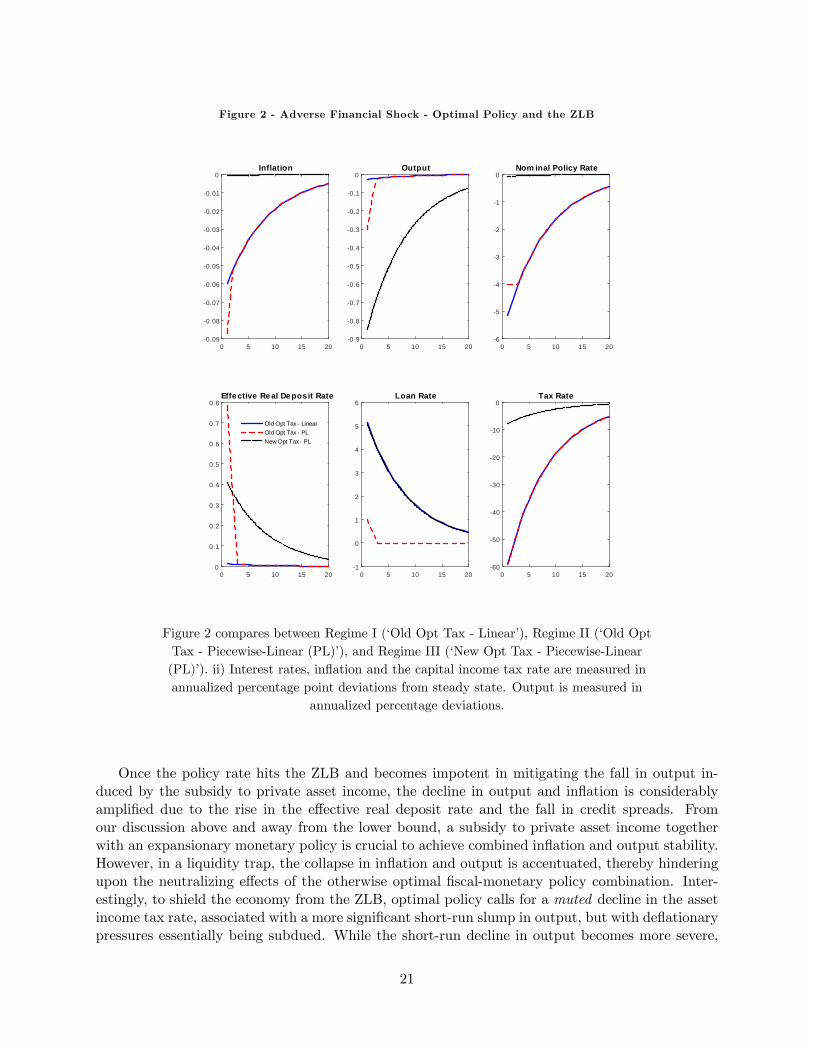
Figure 2 - Adverse Financial Shock - Optimal Policy and the ZLB

0 5 10 15 20­0.09

­0.08

­0.07

­0.06

­0.05

­0.04

­0.03

­0.02

­0.01

0Inflation

0 5 10 15 20­0.9

­0.8

­0.7

­0.6

­0.5

­0.4

­0.3

­0.2

­0.1

0Output

0 5 10 15 20­6

­5

­4

­3

­2

­1

0Nom inal Policy Rate

0 5 10 15 200

0.1

0.2

0.3

0.4

0.5

0.6

0.7

0.8Effective  Real Deposit Rate

0 5 10 15 20­1

0

1

2

3

4

5

6Loan Rate

0 5 10 15 20­60

­50

­40

­30

­20

­10

0Tax Rate

Old Opt Tax ­ LinearOld Opt Tax ­ PLNew Opt Tax ­ PL

Figure 2 compares between Regime I (‘Old Opt Tax - Linear’), Regime II (‘Old OptTax - Piecewise-Linear (PL)’), and Regime III (‘New Opt Tax - Piecewise-Linear(PL)’). ii) Interest rates, inflation and the capital income tax rate are measured inannualized percentage point deviations from steady state. Output is measured in

annualized percentage deviations.

Once the policy rate hits the ZLB and becomes impotent in mitigating the fall in output in-duced by the subsidy to private asset income, the decline in output and inflation is considerablyamplified due to the rise in the effective real deposit rate and the fall in credit spreads. Fromour discussion above and away from the lower bound, a subsidy to private asset income togetherwith an expansionary monetary policy is crucial to achieve combined inflation and output stability.However, in a liquidity trap, the collapse in inflation and output is accentuated, thereby hinderingupon the neutralizing effects of the otherwise optimal fiscal-monetary policy combination. Inter-estingly, to shield the economy from the ZLB, optimal policy calls for a muted decline in the assetincome tax rate, associated with a more significant short-run slump in output, but with deflationarypressures essentially being subdued. While the short-run decline in output becomes more severe,

21

such an optimal policy as described in Regime III minimizes the asymptotic standard deviationsin inflation and GDP, as well reduces the long-run risk of entering a liquidity trap to zero. Table 3summarizes the above discussion, and quantifies the welfare losses from Regimes II and III relativeto the unconstrained Regime I. This table also shows the asymptotic standard deviations in keyvariables and the probability of reaching the ZLB under the different policy regimes.

Table 3: Optimal policy, standard deviations and welfare costs at the ZLB

Regime I Regime II Regime III

s.d (πt) = 0.083

s.d(Yt) = 0.036

s.d (πt) = 1.862

s.d(Yt) = 2.488

s.d (πt) = 1.1× 10−3

s.d(Yt) = 1.183

Probability of hitting ZLB (percent) − 23.90 0Welfare Cost/Gain − −0.2061 −0.0101

Notes: i) The standard deviations of key variables are represented in annualized rates.ii) The welfare cost is the percentage consumption equivalent, measured relative to Regime I - ‘Linear’model.

To conclude, the policy implications of our model following a negative financial shock are fairlyconsistent with what may have been in the minds of policy makers during the peak of the financialcrisis in 2008, when liquidity injections to the banking system and unconventional expansionaryfiscal policies became operative, and the federal funds rate was lowered substantially. While thismodel does not explicitly account for liquidity injections, central bank’s balance sheet policies orthe interest payment on reserves, all of which facilitate bank liquidity, a tax cut on capital incomein this framework is in line with such operations. The policy rate pushed closer towards theZLB is quantitatively also supported by this model. Our counterfactual analysis suggests that theinteraction between unconventional banking taxation (or subsidy) policies and standard monetarypolicy is crucial and can be utilized to counteract the welfare detrimental effects of an inflationaryfinancial shock, at least when the policy rate is away from its lower bound. However, and mostimportantly, following larger financial shocks, the optimal fiscal-monetary policy mix can send theeconomy to a liquidity trap, which then requires a more moderated fall in the savings incometax rate in order to prevent the occurrence of the ZLB. Our model therefore suggests that theuncertainty regarding the size of the shock can hamper the effectiveness of an otherwise optimalfiscal-monetary expansionary policy combination. In fact, such policy can significantly increase therisk of entering an unintended liquidity trap if the policy maker miscalculates the magnitude of thecredit shock.

5.2 Demand Shocks

We now turn to examine the implications of the lower bound on the dynamics and standard devia-tions of key variables, as well as the stabilization properties of optimal capital taxation in a liquiditytrap environment generated by a large negative preference shock. In studying the dynamics of keyvariables following a sizeable adverse demand shock, we also restrict credit spreads from fallingbelow zero so RLt ≥ RDt or RLt − RDt = max(RLt − RDt , 0). Hence, we solve the model with twooccasionally binding constraints, one for the main policy rate and the other for credit spreads.

22

The optimal ZLB capital income tax rate is obtained from the optimization of (34) subject to(32) and (33) with respect to τD,Zt . This problem yields,

τD,Zt = −(1− τD

)τD

(1− β)−1 ret . (37)

Therefore, the optimal tax rate is independent of φπ, and can completely minimize welfare lossesfollowing preference shocks. Optimal policy calls for increasing the tax rate in the face of an adversedemand disturbance (ret < 0) that drives the economy into a liquidity trap.

To illustrate the intuition behind this result, we study the effects of a sizeable adverse preferenceshock that creates a negative co-movement between inflation and output, such that the central banklowers the policy rate until the ZLB constraint becomes binding. For this purpose, we examinea preference shock with a magnitude of 5 × s.d(αϑ), with s.d(αϑ) = 0.009 remaining constant.The multiplicative scale of the shock is set to cause the economy to reach a liquidity trap uponimpact, and stay there for 6 periods (under a benchmark monetary policy rule: φπ = 2 and φ = 0).Admittedly, the duration of the ZLB on the policy rate in our model is shorter than the one observedfor the United States and the Eurozone for nearly a decade (see also Carrillo and Poilly (2013)).Nevertheless, given our parameterization choices and with s.d(αϑ) = 0.009, our model attains theZLB with a frequency of 9 percent, consistent with long-run empirical evidence.

Figure 3 shows the response of key variables to a negative unexpected large preference shock thatdrags the economy into a liquidity trap. The figure compares between three different scenarios:i) Scenario I (‘Linear’) - a standard Taylor rule (φπ = 2) that disregards the lower bound; ii)Scenario II (‘Piecewise (PL)’) - a piecewise-linear solution where the policy rate and credit spreadsare occasionally struck by their lower bound; iii) Scenario III (‘Piecewise (PL)+Optimal Tax Policy(Opt Tax)’) - a piecewise-linear solution where the lower bound may be occasionally binding, therefinance rate follows a standard rule, and the tax rate set according to (37).

23

Figure 3 - Adverse Preference Shock - Liquidity Trap

0 5 10 15 20­5

­4

­3

­2

­1

0Inflation

0 5 10 15 20­3

­2.5

­2

­1.5

­1

­0.5

0

0.5Output

0 5 10 15 20­8

­7

­6

­5

­4

­3

­2

­1

0Nominal Policy Rate

0 5 10 15 20­2.5

­2

­1.5

­1

­0.5

0

0.5

1

1.5Effective Real Deposit Rate

0 5 10 15 20­2.5

­2

­1.5

­1

­0.5

0

0.5Credit Spreads

0 5 10 15 200

5

10

15

20

25

30

35

40Tax Rate

LinearPLPL+Opt Tax

Figure 3 compares between Scenario I (linear model - ‘Linear’), Scenario II(piecewise-linear model - ‘PL’), and Scenario III (piecewise-linear model with optimalcapital taxation - ‘PL+Opt Tax’). ii) Interest rates, credit spreads, inflation and thecapital income tax rate are measured in annualized percentage point deviations from

steady state. Output is measured in annualized percentage deviations.

In Scenario I, an adverse demand shock delivers a direct dip in GDP, which leads to a plummetin prices through a standard demand channel affecting the NKPC, and also to a decline in therisk premium. The fall in the latter acts to lower credit spreads and therefore exacerbate pricedeflation via the credit cost channel. In response to the falling price level, and without the lowerbound being imposed on the policy rate and credit spreads, the central bank lowers the (shadow)policy rate, giving rise to two conflicting effects on the economic activity. On the one hand, a moredrastic cut in the nominal policy rate amplifies deflation due to the direct monetary policy costchannel mechanism. On the other, such an expansionary monetary policy cushions the drop inoutput and hence in inflation. Given our standard parameterization, the direct demand effect ofGDP on inflation dominates such that output declines, prices decrease and the main interest rates

24

are lowered. Therefore, following a preference shock, credit spreads are procyclical with respect tooutput, as opposed to the consequences arising from a financial shock.27

As is evident from Figure 3, there is a striking difference in the behaviour of macro and financialvariables implied by the piecewise-linear Scenario II compared to the linear Scenario I. The fall ininflation and output is more pronounced when the policy rate and credit spreads are constrainedby their lower bound and are thus unable to further adjust in order to mitigate the slump inoutput. Because the demand channel of monetary policy dominates its cost channel mechanism,the central bank would find it welfare-enhancing to cut the refinance rate more substantially despitethe deflationary effects linked with the monetary policy cost channel. However, as the central bankcannot accommodate for the decline in output and inflation using the policy rate alone, the effectivereal policy rate increases, thereby generating a prolonged and aggravated economic recession.

Under the piecewise-linear Scenario III, we find that a liquidity trap can be prevented with theimplementation of an optimal contractionary tax policy. Intuitively, taxation on households wealthrenders the policy maker an extra degree of freedom in seeking its primary objectives via the riskpremium component of the credit cost channel (see also (23), (24), (25)). Commitment to a highertax rate over the course of the shock encourages an expansion in output and a rise in the loan rate,two mechanisms that contribute to restoring the target level of inflation. As a result, the rise inprices also averts the policy rate from tumbling into the ZLB, consequently inducing downwardpressure on the effective real policy rate faced by households and reinforcing the improvement inthe economic activity. In this way, an automatic increase in capital taxation that counteracts anegative demand shock (as implied by (37)) releases the policy rate and credit spreads from thelower bound territory, and insulates the economy from the repercussions of a liquidity trap bothin the short and long-run. Hence, the optimal tax policy can be considered also as a bankingsector tax instrument that is aimed at bringing down the effective real policy rate and increasingborrowing costs against the backdrop of deflationary pressures.

The differences between the three various scenarios are further reflected in Table 4. This tableshows the simulated standard deviations in key variables, the probability of attaining the ZLB, andthe relative welfare cost/gain of the piecewise-linear model without and with optimal tax policycompared to the unconstrained linear case. Interestingly, a significant rise in the tax on net depositreturns of around 37 percentage points following a 5× s.d(αϑ) shock completely insures against aliquidity trap, minimizes the standard deviations in key macro variables, and achieves a meaningfulwelfare benefit of 0.1234 percent.

Table 4: Standard deviations and welfare gains from optimal policy at the lower bound

Linear Piecewise-Linear Piecewise-Linear - Optimal Tax

s.d (πt) = 1.672

s.d(Yt) = 0.186

s.d (πt) = 1.712

s.d(Yt) = 0.387

s.d (πt) = 0

s.d(Yt) = 0

Probability of hitting ZLB (percent) − 9.00 0Welfare Cost/Gain − −0.0083 0.1234

Notes: i) The standard deviations of key variables are represented in annualized rates.ii) The welfare cost / gain is the percentage consumption equivalent, measured relative to the ‘Linear’scenario.

27De Fiore and Tristani (2013) also find that following some shocks, the risk premium and the cost of borrowingare procyclical with respect to GDP.

25

While this model does not explicitly account for the bank reserves market, the recent implemen-tation of the negative interest on reserves policy by the ECB is equivalent to taxing the bankingsector or lowering the effective savings rate faced by households. Therefore, increasing the tax rateon private asset returns in a liquidity trap, as we advocate for in this model, is not inconsistentwith the recent attempts taken by the ECB to lower deposit rates and to increase credit spreads inlight of the persistent low inflation experienced in the Eurozone. We show that such a policy canbe achieved by varying the tax rate on net asset returns.

5.3 Welfare Gains from Dynamic Tax Regimes

The analysis so far has explored the welfare improving properties of optimal state-contingent privateasset taxation in a stochastic environment. However, as mentioned earlier in the equilibrium section,a positive tax in steady state, τD > 0, induces a lending rate above the level that would prevailwith τD = 0. Such tax is then passed on to IG firms and generates an ineffi cient long-run level ofoutput and thus lower welfare. Therefore, the optimal policy in steady state would be to set a zerocapital tax rate.

This section analyses more broadly the welfare costs and benefits from the optimal dynamicbehaviour of asset taxation, as discussed in the previous sections, against a regime where τDt = 0for all t. In a deterministic environment, the regime absent of savings taxation is always preferreddue the mitigated distortions transmitted from the lending rate to output. In a stochastic en-vironment, nonetheless, the relative welfare gains of state-contingent asset taxation, used as anadditional instrument to smooth the business cycle and to mitigate welfare losses, depend on thetype and volatility of the shock hitting the economy. As shock volatilities increase, so do therelative welfare gains from the additional degree of freedom arising from the implementation ofunconventional dynamic taxation. In other words, the welfare gains from applying state-contingenttaxation overcomes the steady state welfare losses induced by setting τDt 6= 0.

26

Figure 4 - Shock Volatilities, Dynamic Taxation and Welfare

0.01 0.02 0.03 0.04 0.05 0.06 0.07 0.08 0.09Shock Volatilities ­ Financial Shock

­1

­0.5

0

0.5

1

1.5

2

Wel

fare

 Gai

ns fr

om T

ax R

egim

e

10­3

Financial ShockDemand Shock

0 0.5 1 1.5 2 2.5 3 3.5 4 4.5 5Shock Volatilities ­ Demand Shock

10­3

Note: The top horizontal axis measures the shock volatilities for demand shock,whereas the bottom horizontal axis represents the financial shock volatilities.

Figure 4 indeed confirms that for financial shocks with volatilities above 0.045, and for prefer-ence shock with volatilities higher than 0.004, the welfare gains from varying private asset taxationare strictly positive. These standard deviations thresholds are significantly lower than empiricalestimates found in Christiano, Motto and Rostagno (2014), and Denes, Eggertsson and Gilbukh(2013), among others. Therefore, we advocate for tax flexibility, associated with higher tax volatil-ity, to shield the economy from the repercussions of volatile shocks that can result in liquidity trapepisodes and significant welfare losses. Contributing to Eggertsson (2011), who mainly focuses onfiscal policy multipliers, we quantify the welfare gains of unconventional optimal taxation policiesand find the optimal capital tax rate that can be used as an automatic stabilizer in the presence ofboth financial and demand shocks.

6 Concluding Remarks

By employing a standard three-equation New Keynesian model modified for a credit cost channel,endogenous financial risk, a banking sector and the lower bound, we shed new insights on thewelfare implications, stabilization properties and transmission mechanisms of optimal private assettaxation. We show that varying capital taxation according to the state of the business and financialcycles has meaningful effects on the behaviour of macroeconomic and financial variables, and altersthe transmission of standard monetary policy. The distinctive risk premium channel highlightedin our model presents an additional motivation for applying state-contingent capital taxation byaffording the policy maker an extra degree of freedom to pursue its primary mandates. Our modelsupports the use of state-contingent capital taxation policies and specifically the implementation of

27

subsidies to the banking sector following inflationary financial shocks, and taxing households liquidprivate assets against the backdrop of deflationary demand shocks.

This paper also advances an alternative answer to the highly topical question: how can aliquidity trap be avoided, and which optimal policies can help to achieve this goal? Blanchard,Dell’Ariccia and Mauro (2010) propose increasing the inflation target, as well as argue for a betterintegration between monetary and fiscal policy. Nakov (2008) suggests to change the monetarypolicy strategy such that in times of low inflation the central bank promises to raise inflation toits target level. Finally, Adam and Billi (2007) put forward the idea to increase the aggressivenessof monetary policy in order to reduce the probability of hitting the ZLB. Contributing to thisliterature, we advocate for cyclically adjusting the tax on asset returns based on the nature and scaleof the shock hitting the economy, and show how financial frictions, liquidity traps and monetarypolicy modify the behaviour of such unconventional taxation policy.

Like Correia, Farhi, Nicolini, and Teles (2013), our state-contingent policy recommendationsrequire taxes to be flexible and rather volatile. It is well known that fiscal policy tools are notas flexible as monetary policy instruments, and require a long legislative process until they canactually be executed. The recent Great Recession, however, has led to somewhat more flexibility interms of implementing fiscal and financial policies, despite the main focus still placed on governmentspending since the American Recovery and Reinvestment Act (ARRA) of 2009, and countercyclicalregulation associated with the gradual imposition of Basel III. Either way, we make a normativepoint that taxes (or financial policies) should be at least as flexible as monetary policy, so long asthe policy maker can correctly identify the source and the size of the shock distorting the economy.

28

References

[1] Adam, Klaus, and Roberto M. Billi. (2007). "Discretionary monetary policy and the zero lowerbound on nominal interest rates", Journal of Monetary Economics, 54(3), 728-752.

[2] Agénor, Pierre-Richard, and Joshua Aizenman. (1998). “Contagion and Volatility with Imper-fect Credit Markets”, International Monetary Fund Staff Papers, 45, 207-235.

[3] Amano, Robert, and Malik Shukayev. (2012). "Risk premium shocks and the zero bound onnominal interest rates", Journal of Money, Credit and Banking, 44(8), 1475-1505.

[4] Barro, Robert (2009). “Government Spending Is No Free Lunch”, Wall Street Journal, January22, Opinion page.

[5] Benes, Jaromir, and Michael Kumhof. (2015). "Risky Bank Lending and Countercyclical Cap-ital Buffers", Journal of Economic Dynamics and Control, 58, 58—80.

[6] Bernanke, Ben S., Mark Gertler, and Simon Gilchrist. (1999). "The financial accelerator in aquantitative business cycle framework", Handbook of Macroeconomics, 1, 1341-1393.

[7] Blanchard, Olivier, Giovanni Dell’Ariccia, and Paolo Mauro. (2010). "Rethinking macroeco-nomic policy", Journal of Money, Credit and Banking, 42(s1), 99-215.

[8] Calvo, Guillermo A. (1983). “Staggered Prices in a Utility-Maximizing Framework”, Journalof Monetary Economics, 12, 383-398.

[9] Carlstrom, Charles T., and Timothy S. Fuerst. (1997). "Agency costs, net worth, and businessfluctuations: A computable general equilibrium analysis", American Economic Review, 87,893-910.

[10] Carrillo, Julio A., and Céline Poilly. (2013). "How do financial frictions affect the spendingmultiplier during a liquidity trap?", Review of Economic Dynamics, 16(2), 296-311.

[11] Chamley, Christophe. (1986). "Optimal taxation of capital income in general equilibrium withinfinite lives", Econometrica, 54(3), 607-622.

[12] Chari, Varadarajan V., Lawrence J. Christiano, and Patrick J. Kehoe. (1994). "Optimal fiscalpolicy in a business cycle model", Journal of Polítical Economy, 102(4), 617-652.

[13] Christensen, Ian, and Ali Dib. (2008). "Monetary policy in an estimated DSGE model with afinancial accelerator". Review of Economic Dynamics, 11, 155—178.

[14] Christiano, Lawrence J., Roberto Motto and, Massimo Rostagno. (2014). "Risk Shocks", Amer-ican Economic Review, 104(1), 27-65.

[15] Christiano, Lawrence J., Martin Eichenbaum, and Sergio Rebelo. (2011). “When is the gov-ernment spending multiplier large?”, Journal of Political Economy, 119(1), 78-121.

[16] Christiano, Lawrence J., Martin S. Eichenbaum, and Mathias Trabandt. (2015). “Understand-ing the Great Recession”, American Economic Journal: Macroeconomics, 7(1), 110—167.

[17] Collard, Fabrice, Harris Dellas, Behzad Diba, and Olivier Loisel. (2017). "Optimal monetaryand prudential policies", American Economic Journal: Macroeconomics, 9(1), 40-87.

29

[18] Conti, Antonio Maria, Stefano Neri, and Andrea Nobili. (2016).“Low Inflation and monetarypolicy in the euro area”, Bank of Italy Working Paper no. 1019.

[19] Correia, Isabel, Emmanuel Farhi, Juan Pablo Nicolini, and Pedro Teles. (2013). “Unconven-tional Fiscal Policy at the Zero Bound”. American Economic Review, 103(4), 1172-1211.

[20] Cúrdia, Vasco, and Michael Woodford. (2010). "Credit Spreads and Monetary Policy", Journalof Money, Credit and Banking, 42(s1), 3-35.

[21] Cúrdia, Vasco, and Michael Woodford. (2016). "Credit Frictions and Optimal Monetary Pol-icy", Journal of Monetary Economics, 84, 30-65.

[22] De Graeve, Ferre. (2008). "The external finance premium and the macroeconomy: US post-WWII evidence", Journal of Economic Dynamics and Control, 32(11), 3415-3440.

[23] De Fiore, Fiorella, and Oreste Tristani. (2013). “Optimal Monetary Policy in a Model of theCredit Channel”, The Economic Journal, 123(571), 906-931.

[24] De Paoli, Bianca, and Matthias Paustian. (2017). “Coordinating Monetary and Macropruden-tial Policies”, Journal of Money, Credit and Banking, 49 (2-3), 319-349.

[25] Demirel, Ufuk D. (2009). "Optimal monetary policy in a financially fragile economy", TheB.E. Journal of Macroeconomics, 9(1), Article 15.

[26] Denes, Matthew, Gauti B. Eggertsson, and Sophia Gilbukh. (2013). "Deficits, public debtdynamics and tax and spending multipliers", The Economic Journal, 123(566), F133-F163.

[27] Dixit, Avinash K., and Joseph E. Stiglitz. (1977). “Monopolistic Competition and OptimumProduct Diversity”, American Economic Review, 67, 297-308.

[28] Drautzburg, Thorsten, and Harald Uhlig. (2015). "Fiscal stimulus and distortionary taxation",Review of Economic Dynamics, 18(4), 894-920.

[29] Eggertsson, Gauti B. (2011). "What fiscal policy is effective at zero interest rates?", NBERMacroeconomics Annual 2010, 25, 59-112.

[30] Eggertsson, Gauti B., and Michael Woodford. (2006). “Optimal Monetary and Fiscal Policy ina Liquidity Trap”. In NBER International Seminar on Macroeconomics 2004, edited by RichardH. Clarida, Jeffrey Frankel, Francesco Giavazzi, and Kenneth D. West, 75—144. Cambridge,MA: MIT Press.

[31] Faia, Ester, and Tommaso Monacelli. (2007). "Optimal interest rate rules, asset prices, andcredit frictions", Journal of Economic Dynamics and Control, 31(10), 3228-3254.

[32] Feldstein, Martin S. (2009). “Rethinking the Role of Fiscal Policy”, American Economic Re-view, 99(2), 556—559.

[33] Fernández-Villaverde, Jesús. (2010). "Fiscal policy in a model with financial frictions", Amer-ican Economic Review Papers and Proceedings, 100(2), 35-40.

[34] Gomes, Joao F., Amir Yaron, and Lu Zhang. (2003). "Asset prices and business cycles withcostly external finance", Review of Economic Dynamics, 6(4), 767-788.

30

[35] Goodfriend, Marvin, and Bennett T. McCallum. (2007). "Banking and interest rates in mon-etary policy analysis: A quantitative exploration", Journal of Monetary Economics, 54(5),1480-1507.

[36] Gilchrist, Simon, Raphael Schoenle, Jae Sim, and Egon Zakrajsek. (2017). “Inflation DynamicsDuring the Financial Crisis”, American Economic Review, 107(3), 785-823.

[37] Gilchrist, Simon, and Egon Zakrajšek. (2012). "Credit spreads and business cycle fluctuations",American Economic Review, 102(4), 1692-1720.

[38] Guerrieri, Luca, and Matteo Iacoviello. (2015). "OccBin: A toolkit for solving dynamic modelswith occasionally binding constraints easily", Journal of Monetary Economics, 70, 22-38.

[39] Holden, Tom. (2016). “Computation of solutions to dynamic models with occasionally bindingconstraints”, University of Surrey.

[40] Judd, Kenneth L. (1985). "Redistributive taxation in a simple perfect foresight model", Journalof Public Economics, 28(1), 59-83.

[41] Mertens, Karel RSM, and Morten O. Ravn. (2014). "Fiscal policy in an expectations-drivenliquidity trap", The Review of Economic Studies, 81(4), 1637—1667.

[42] Nakata, Taisuke. (2016). "Optimal fiscal and monetary policy with occasionally binding zerobound constraints", Journal of Economic Dynamics and Control, 73, 220-240.

[43] Nakov, Anton. (2008). "Optimal and simple monetary policy rules with zero floor on thenominal interest rate", International Journal of Central Banking, 4(2), 73—127.

[44] Ravenna, Federico, and Carl E. Walsh. (2006). “Optimal Monetary Policy with the CostChannel”, Journal of Monetary Economics, 53, 199-216.

[45] Tayler, William J., and Roy Zilberman. (2016). "Macroprudential regulation, credit spreadsand the role of monetary policy", Journal of Financial Stability, 26(c), 144-158.

[46] Taylor, John B. (1993). “Discretion versus Policy Rules in Practice”, Carnegie-Rochester Con-ference Series on Public Policy, 39, 195-214.

[47] Uhlig, Harald. (2010). "Some fiscal calculus", American Economic Review, 100(2), 30-34.

[48] Woodford, Michael. (2003). “Interest and Prices: Foundations of a Theory of Monetary Policy”,Princeton, NJ: Princeton University Press.

[49] Woodford, Michael. (2011). "Simple analytics of the government expenditure multiplier",American Economic Journal: Macroeconomics, 3(1), 1-35.

31

7 Appendix - Welfare Function Derivation (Not for publication)

The derivation of the loss function as presented in the paper strictly follows Woodford (2003) andRavenna and Walsh (2006, online appendix).

To derive a second-order approximation of the representative utility function, it is first necessaryto clarify some additional notation. For any variable Xt, let X be its steady state value, Xet be itseffi cient level, Xt = Xt−X be the deviation of Xt around its steady state, and finally Xt = log(Xt/X)be the log-deviation of Xt around its correspondent steady state. Using a second order Taylorapproximation, the variables Xt and X can be related using the following equation,

XtX

= 1 + log

(XtX

)+

1

2

[log

(XtX

)]2

= 1 + Xt +1

2X2t . (38)

As we can write Xt = X(XtX − 1

), it follows that Xt ≈ X

(Xt + 1

2 X2t

).

Utility is assumed to be separable in consumption and leisure,

Ut = Et∞∑t=0

βt

{ϑtC

1−ςt

1− ς −ϑtH

1+γt

1 + γ

}. (39)

We start by approximating the utility from consumption. With the steady state value of thediscount factor shock (ϑ) equal to 1, the second order expansion for U(Ct, ϑt) yields,

U(Ct, ϑt) ≈ U(C, 1) + UC(C, 1)Ct +1

2UCC(C, 1)C2

t +

Uϑ(C, 1)ϑt +1

2Uϑ,ϑϑ

2

t + UC,ϑϑtCt, (40)

which according to our utility function (39) results in,

U(Ct, ϑt) ≈ U(C, 1) + UC(C, 1)Ct +1

2UCC(C, 1)C2

t +

Uϑ(C, 1)ϑt +1

2Uϑ,ϑϑ

2

t + UC,ϑϑtCt,

using ϑt ≈ ϑt and UC,ϑ = UC(C, 1), the above becomes,

U(Ct, ϑt) ≈ U(C, 1) + UC(C, 1)C

(Ct +

1

2C2t

)− 1

2ςUC(C, 1)C

(Ct +

1

2C2t

)2

+

+Uϑ(C, 1)ϑt +1

2Uϑ,ϑϑ

2

t + UC(C, 1)Cϑt

(Ct +

1

2C2t

),

ignoring the terms Xi for i > 2 yields,

U(Ct, ϑt) ≈ U(C, 1) + UC(C, 1)C

[(1 + ϑt

)Ct +

1

2(1− ς) C2

t

]+

+Uϑ(C, 1)ϑt +1

2Uϑ,ϑϑ

2

t , (41)

32

We next derive an expression for the disutility from labour. The Taylor expansion for V (Ht, ϑt)gives,

V (Ht, ϑt) ≈ V (H, 1) + VH(H, 1)Ht +1

2VHH(H, 1)H2

t +

+Vϑ(C, 1)ϑt +1

2Vϑ,ϑϑ

2

t + VC,ϑϑtHt, (42)

where aggregate employment is,

Ht =

1∫0

Hj,tdj,

and employment at firm j,

Hj,t ≈ H[Hj,t +

1

2H2j,t

].

For the purpose of calculating the ex-ante loss function, we ignore the effects of the idiosyncraticshock that takes place at the end of the period such that εj,t = 0. We therefore only examine theex-ante uniform properties of this shock to calculate welfare. Using this assumption, each firm facesthe following technology function,

Hj,t = Yj,t.

Thus, we can define employment as,

Ht = H

1∫0

Yj,tdj +1

2

1∫0

Y 2j,tdj

. (43)

Substituting (43) into (42) and using H = Y results in,

V (Ht, ϑt) ≈ V (Y, 1) + VH(Y, 1)Y

1∫0

Yj,tdj +1

2

1∫0

Y 2j,tdj

+

+1

2VHH(Y, 1)Y 2

1∫0

Yj,tdj

2

+ Vϑ(C, 1)

(ϑt +

1

2ϑ

2

t

)+

+1

2Vϑ,ϑ

(ϑt +

1

2ϑ

2

t

)2

+

+VH,ϑY

(ϑt +

1

2ϑ

2

t

) 1∫0

Yj,tdj +1

2

1∫0

Y 2j,tdj

.

33

ignoring terms of Xi for i > 2 yields,

V (Ht, ϑt) ≈ V (Y, 1) + VH(Y, 1)Y

1∫0

Yj,tdj +1

2

1∫0

Y 2j,tdj

+

+1

2VHH(Y, 1)Y 2

1∫0

Yj,tdj

2

+

+Vϑ(Y, 1)ϑt +1

2Vϑ,ϑϑ

2

t + VH,ϑY ϑt

1∫0

Yj,tdj. (44)

Given the demand function of each firm j, aggregate output is approximated by,

Yt =

1∫0

Yj,tdj +1

2

(λ− 1

λ

)varj Yj,t,

hence, 1∫0

Yj,tdj

2

=

[Yt −

1

2

(λ− 1

λ

)varj Yj,t

]2

≈ Y 2t ,

and,1∫

0

Y 2j,tdj =

1∫0

Yj,tdj

2

+ varj Yj,t.

Therefore,1∫

0

Y 2j,tdj ≈ Y 2

t + varj Yj,t,

and,1∫

0

Yj,tdj ≈ Yt.

Using VH,ϑ = VH(Y, 1) and the above results, (44) becomes,

V (Ht, ϑt) ≈ V (Y, 1) + VH(Y, 1)Y

{(1 + ϑt

)Yt +

1

2

(1

λ

)varj Yj,t +

1

2(1 + γ) Y 2

t

}+ (45)

+Vϑ(Y, 1)ϑt +1

2Vϑ,ϑϑ

2

t

34

To determine total utility we subtract (45) from (41) to obtain,

U(Ct, ϑt)− V (Ht, ϑt) = U(C, 1)− V (Y, 1) + UC(C, 1)C

[(1 + ϑt

)Ct +

1

2(1− ς) C2

t

]−

−VH(Y, 1)Y

{(1 + ϑt

)Yt +

1

2

(1

λ

)varj Yj,t +

1

2(1 + γ) Y 2

t

}+ (Uϑ(C, 1)− Vϑ(Y, 1)) ϑt +

1

2(Uϑ,ϑ − Vϑ,ϑ) ϑ

2

t . (46)

Note that the steady state labour market equilibrium condition is VHUC = W = µε(pm)RL

, where µε = 1

is the average of the idiosyncratic shock, and pm ≡ λ(λ−1) is the price mark-up. We define Ξ such

that,

1− Ξ ≡ 1

(pm)RL.

Then VH(H, 1)Y can be written as UC (C, 1)Y (1−Ξ). As in Ravenna and Walsh (2006), given thatthe Ξ is small, terms such as (1− Ξ)Y 2 simply boil down to Y 2

t .28 With these assumption we can

now rewrite equation (46) as,

U(Ct, ϑt)− V (Ht, ϑt) = U(C, 1)− V (Y, 1) + UC(C, 1)C

[(1 + ϑt

)Ct +

1

2(1− ς) C2

t

]−

−UC (C, 1)Y (1− Ξ)

[ (1 + ϑt

)Yt+

+12

(1λ

)varj Yj,t + 1

2 (1 + γ) Y 2t

]+

+ (Uϑ(C, 1)− Vϑ(Y, 1)) ϑt +1

2(Uϑ,ϑ − Vϑ,ϑ) ϑ

2

t . (47)

Using C = Y and collecting terms,

U(Ct, ϑt)− V (Ht, ϑt) = U(C, 1)− V (Y, 1)

+UC(C, 1)Y

{ (1 + ϑt

) [Ct − (1− Ξ)Yt

]+

+12 (1− ς) C2

t − 12 (1 + γ) Y 2

t

}

−1

2UC(C, 1)Y

(1

λ

)varj Yj,t +

+ (Uϑ(C, 1)− Vϑ(Y, 1)) ϑt +1

2(Uϑ,ϑ − Vϑ,ϑ) ϑ

2

t

28Note that like Ravenna and Walsh (2006), the value of Ξ is increasing with the price markup and the loan rate,which in our model is larger due to the presence of the various financial frictions.

35

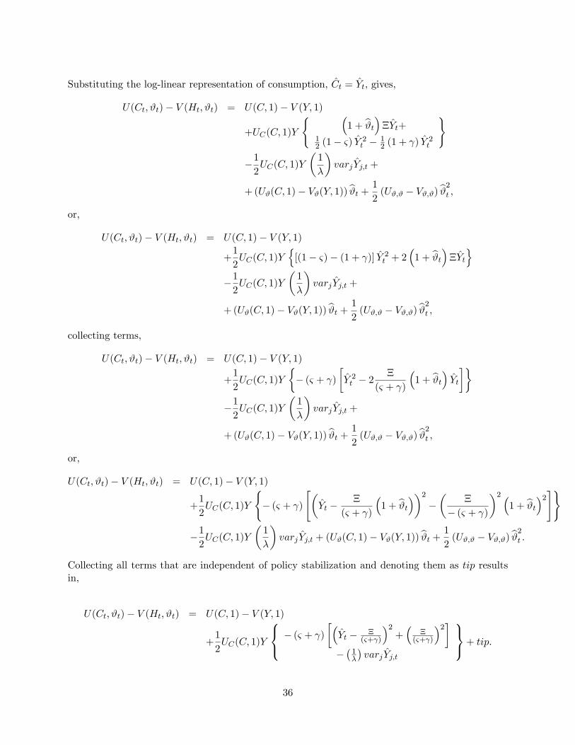
Substituting the log-linear representation of consumption, Ct = Yt, gives,

U(Ct, ϑt)− V (Ht, ϑt) = U(C, 1)− V (Y, 1)

+UC(C, 1)Y

{ (1 + ϑt

)ΞYt+

12 (1− ς) Y 2

t − 12 (1 + γ) Y 2

t

}

−1

2UC(C, 1)Y

(1

λ

)varj Yj,t +

+ (Uϑ(C, 1)− Vϑ(Y, 1)) ϑt +1

2(Uϑ,ϑ − Vϑ,ϑ) ϑ

2

t ,

or,

U(Ct, ϑt)− V (Ht, ϑt) = U(C, 1)− V (Y, 1)

+1

2UC(C, 1)Y

{[(1− ς)− (1 + γ)] Y 2

t + 2(

1 + ϑt

)ΞYt

}−1

2UC(C, 1)Y

(1

λ

)varj Yj,t +

+ (Uϑ(C, 1)− Vϑ(Y, 1)) ϑt +1

2(Uϑ,ϑ − Vϑ,ϑ) ϑ

2

t ,

collecting terms,

U(Ct, ϑt)− V (Ht, ϑt) = U(C, 1)− V (Y, 1)

+1

2UC(C, 1)Y

{− (ς + γ)

[Y 2t − 2

Ξ

(ς + γ)

(1 + ϑt

)Yt

]}−1

2UC(C, 1)Y

(1

λ

)varj Yj,t +

+ (Uϑ(C, 1)− Vϑ(Y, 1)) ϑt +1

2(Uϑ,ϑ − Vϑ,ϑ) ϑ

2

t ,

or,

U(Ct, ϑt)− V (Ht, ϑt) = U(C, 1)− V (Y, 1)

+1

2UC(C, 1)Y

{− (ς + γ)

[(Yt −

Ξ

(ς + γ)

(1 + ϑt

))2

−(

Ξ

− (ς + γ)

)2 (1 + ϑt

)2]}

−1

2UC(C, 1)Y

(1

λ

)varj Yj,t + (Uϑ(C, 1)− Vϑ(Y, 1)) ϑt +

1

2(Uϑ,ϑ − Vϑ,ϑ) ϑ

2

t .

Collecting all terms that are independent of policy stabilization and denoting them as tip resultsin,

U(Ct, ϑt)− V (Ht, ϑt) = U(C, 1)− V (Y, 1)

+1

2UC(C, 1)Y

− (ς + γ)

[(Yt − Ξ

(ς+γ)

)2+(

Ξ(ς+γ)

)2]

−(

1λ

)varj Yj,t

+ tip.

36

Assuming that the term Ξ(ς+γ) is a small constant, the above boils down to,

U(Ct, ϑt)− V (Ht, ϑt) = U(C, 1)− V (Y, 1)

+1

2UC(C, 1)Y

{− (ς + γ) Y 2

t −(

1

λ

)varj Yj,t

}+ tip. (48)

Given the demand function for each intermediate good, Yj,t = Yt

(Pj,tPt

)−λ, we have,

log Yj,t = log Yt − λ (logPj,t − logPt) ,

so,varj log Yj,t = λ2varj logPj,t.

Note the price adjustment mechanism involves a randomly chosen fraction (1− ω) of all firms actingoptimally by adjusting prices in each period. Defining ∆t ≡ varj logPj,t then Woodford (2003, pp.694-696) shows that,

∆t ≈ ω∆t−1 +

(ω

1− ω

)π2t .

Assuming ∆t−1 is the initial degree of price dispersion, then,

∞∑t=0

βtt∆t =

[ω

(1− ω) (1− ωβ)

] ∞∑t=0

βtπ2t + tip. (49)

Combining (49) with (48), the present discounted value of the representative household welfare is,

Wt≡∞∑t=0

βtUt ≈ U −∞∑t=0

βtLt,

where the associated losses from welfare are given by,

∞∑t=0

βtLt =1

2UC(C, 1)Y E0

∞∑t=0

βt[(

λ

κp

)π2t + (ς + γ) Y 2

t

], (50)

with κp = (1−ω)(1−ωβ)ω . With ς = 1 and Y = C, (50) boils down to,

∞∑t=0

βtLt =1

2E0

∞∑t=0

βt[(

λ

κp

)π2t + (1 + γ) Y 2

t

]. (51)

Welfare MeasureIn considering optimal taxation policies, we measure the welfare benefit of a particular optimal

policy j as a fraction of the consumption path under the benchmark case (Policy I) that must begiven up in order to obtain the benefits of welfare associated with the various optimal policies;

Et∞∑t=0

βtUt

(Cjt , H

jt

)= Et

∞∑t=0

βtUt((1− Λ)CIt , H

It

), where superscript j refers to Policies II and

III and superscript I refers to Policy I. Given the utility function adopted and with ς = 1, the

37

expression for Λ in percentage terms is,

Λ ={

1− exp[(1− β)

(Wjt −WI

t

)]}× 100,

whereWjt = Et

∞∑t=0

βtUt

(Cjt , H

jt

)represents the unconditional expectation of lifetime utility under

policy j = II, III, and WIt = Et

∞∑t=0

βtUt(CIt , H

It

)is the welfare associated with the benchmark

Policy I. Converting the loss function to the welfare measure gives,

Wt≡U −1

2

UCC

(1− β)

[(λ

κp

)var(πt) + (1 + γ) var

(Yt

)].

38