taxation, corruption, and growth - national academies
TRANSCRIPT

Taxation, Corruption, and Growth
William Kerr

Motivation
• It taxation good for growth? – Incentive effects – Public good effects – Redistribution effects
• What role does the efficiency of government play?
• What is the optimum?

Model Structure
• Builds on Klette and Kortum (2004) model – Realistic firm dynamics, entry margin
• Innovation depends on firm’s effort and quality of public infrastructure
• Government collects tax revenue to finance infrastructure investment
• Government efficiency impacts the realized public goods gain from taxes

Our Beloved Firms and Entry
• All firms experience trade-offs: – Better infrastructure lowers firm costs and boosts
returns from innovation investments – Disincentive effects of taxation reduce expected
innovation returns
• Better gov’t efficiency has asymmetric gain in terms of growth
• Entrants display a special sensitivity


Key Theoretical Results
• Inverted-U effect of taxation on growth – Public good effect dominates at low rates – Incentive effect dominates at high rates – Interaction between taxation and government
efficiency is positive for growth to left of peak
• The optimal taxation rate is higher for a more efficiency government

Empirical Approach
• State-level estimations of the model – GDP, employment, growth, etc. – Entrepreneurship/innovation particulars
• Causality? – Granger causality tests – State border effects by isolating counties

Data
• Traditional sources – BEA state data – Longitudinal Business Database (LBD) – NBER patent database – Tax receipts and Taxsim
• Structure – Focus on five-year periods starting 1983 – Within each period, take averages of our outcome
variables for GDP and employment

Lonely Planet: Alabama Obsessed with football and race – two things Southerners never stop discussing – this rectangular state has a complicated and fascinating heritage. […] its reputation of rebels, segregation, discrimination and wayward politicians.

Key Empirical Results
• Basic empirical approach:
• Measure corruption through average number of officials
convicted of federal crimes in the previous period • Measure average income tax revenues collected in the previous
period converted into constant 2000 dollars • Both are normalized by initial state government size

Log tax revenues per 0.183 0.182gov. exp. in prior period (0.096) (0.096)
Log tax revenues per -0.033gov. exp. in prior period SQ (0.024)
Log corruption per -0.017 -0.012gov. exp. in prior period (0.015) (0.019)
Interaction of taxes and -0.060 -0.072corruption in prior period (0.023) (0.040)
Interaction of taxes and -0.021corruption in prior pd. SQ (0.028)
State and period effects Yes YesObservations 188 188
Table 1a: Base estimation for log state GDP

Approximate point of statistical insignificance
from zero effect
Tax percentile:
90th
25th
75th
50th
10th

90th
25th
75th
50th
10th

90th
25th
75th 50th
10th

Log total Log total Log total Log average Log patenting Log patentingemployment employment employment size of of individuals of incumbent
in young in old in entry/exit continuing and firms that firms that areestablishments establishments establishments establishments are younger five years old
in period in period in period in period than five years or more
(1) (2) (3) (4) (5) (6)
Log tax revenues per 0.088 0.160 0.092 0.049 0.085 0.115gov. exp. in prior period (0.110) (0.120) (0.130) (0.032) (0.137) (0.280)
Log corruption per 0.005 -0.008 0.007 0.004 0.003 -0.086gov. exp. in prior period (0.015) (0.015) (0.018) (0.006) (0.038) (0.085)
Interaction of taxes and -0.043 -0.055 -0.045 -0.014 -0.092 -0.075corruption in prior period (0.015) (0.025) (0.018) (0.010) (0.037) (0.076)
State and period effects Yes Yes Yes Yes Yes YesObservations 188 188 188 188 188 188
Table 4: Panel relationship of taxation, corruption and economic activity
Notes: See Table 1a. Column 1 of Table 1a is repeated for various economic outcomes.
Extensions to consider entry vs. incumbent roles

Narrowing WideningBase estimation Counties with Counties with spatial range spatial rangeusing 100 mile Counties that Counties that >50% of local <50% of local from 100 miles from 100 miles
spatial ring border on other do not border employment employment to 50 miles to 200 miles around county states onto other states in other states in other states around county around county
(1) (2) (3) (4) (5) (6) (7)
Log tax revenues per 0.046 0.074 0.046 0.028 0.050 0.034 0.014gov. exp. in prior period (0.047) (0.053) (0.053) (0.098) (0.046) (0.037) (0.051)
Log corruption per 0.009 0.021 0.006 0.038 0.005 0.005 0.007gov. exp. in prior period (0.014) (0.016) (0.015) (0.021) (0.013) (0.011) (0.019)
Interaction of taxes and -0.032 -0.036 -0.035 -0.056 -0.035 -0.022 -0.047corruption in prior period (0.013) (0.024) (0.014) (0.026) (0.013) (0.009) (0.021)
Lagged log county level -0.394 -0.347 -0.428 -0.353 -0.403 -0.395 -0.392in the prior period (0.023) (0.033) (0.028) (0.038) (0.027) (0.024) (0.024)
County and period effects Yes Yes Yes Yes Yes Yes YesObservations 11,180 4,216 6,964 2,853 8,327 11,180 11,180
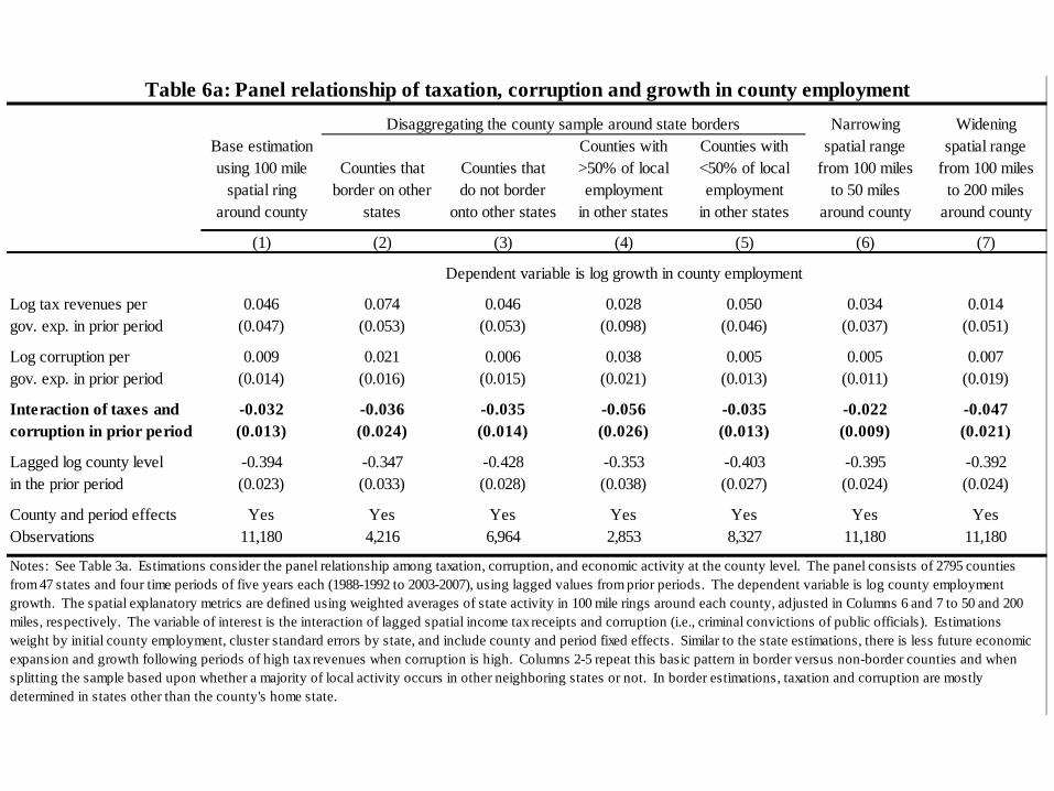
Table 6a: Panel relationship of taxation, corruption and growth in county employment
Notes: See Table 3a. Estimations consider the panel relationship among taxation, corruption, and economic activity at the county level. The panel consists of 2795 counties from 47 states and four time periods of five years each (1988-1992 to 2003-2007), using lagged values from prior periods. The dependent variable is log county employment growth. The spatial explanatory metrics are defined using weighted averages of state activity in 100 mile rings around each county, adjusted in Columns 6 and 7 to 50 and 200 miles, respectively. The variable of interest is the interaction of lagged spatial income tax receipts and corruption (i.e., criminal convictions of public officials). Estimations weight by initial county employment, cluster standard errors by state, and include county and period fixed effects. Similar to the state estimations, there is less future economic expansion and growth following periods of high tax revenues when corruption is high. Columns 2-5 repeat this basic pattern in border versus non-border counties and when splitting the sample based upon whether a majority of local activity occurs in other neighboring states or not. In border estimations, taxation and corruption are mostly determined in states other than the county's home state.
Disaggregating the county sample around state borders
Dependent variable is log growth in county employment

Narrowing WideningBase estimation Counties with Counties with spatial range spatial rangeusing 100 mile Counties that Counties that >50% of local <50% of local from 100 miles from 100 miles
spatial ring border on other do not border employment employment to 50 miles to 200 miles around county states onto other states in other states in other states around county around county
(1) (2) (3) (4) (5) (6) (7)
Log tax revenues per 0.073 0.084 0.068 0.084 0.066 0.043 0.038gov. exp. in prior period (0.031) (0.037) (0.033) (0.047) (0.030) (0.025) (0.038)
Log corruption per 0.002 0.007 0.001 0.026 -0.003 0.000 -0.004gov. exp. in prior period (0.010) (0.010) (0.011) (0.018) (0.010) (0.008) (0.013)
Interaction of taxes and -0.025 -0.042 -0.021 -0.048 -0.023 -0.015 -0.033corruption in prior period (0.008) (0.014) (0.008) (0.033) (0.008) (0.006) (0.015)
Lagged log county level -0.316 -0.325 -0.369 -0.337 -0.297 -0.315 -0.312in the prior period (0.036) (0.037) (0.042) (0.038) (0.045) (0.038) (0.037)
County and period effects Yes Yes Yes Yes Yes Yes YesObservations 11,180 4,216 6,964 2,853 8,327 11,180 11,180
Table 6b: Panel relationship of taxation, corruption and growth in county establishmentsDisaggregating the county sample around state borders
Notes: See Table 6a. The dependent variable is adjusted in these specifications to be log growth in county establishments.
Dependent variable is log growth in county establishments

Calibrated Model
In calibrated framework, US not far off its optimal rate for its level of government efficiency

Calibrated Model
The biggest gains would come from improving efficiency versus tax optimization

Calibrated Model
Entrant share of innovation is increasing in government efficiency and lowering tax rates from current levels

Key Empirical Results
• An inverted-U effect of taxation on growth – The interaction of tax and corruption for growth is
robustly negative
• Marginal effect of taxation on growth: – At <=25th corruption percentile, highly positive
and significant until upper part of US tax range – At 90th corruption percentile, much lower and
soon negative
• Marginal gain largest for better efficiency

Conclusions
• Hopefully making progress on several fronts – Better connections of taxes and growth – Understanding big levers for impact – Thinking through entry’s role
• Much more that can be done – Optimal tax design (progressivity, personal vs.
corporate, etc.) – More detailed considerations of types of
expenditures and growth impact