Taxation and Family Firms1

Wojciech Kopczuk

Columbia University

Joel Slemrod

University of Michigan

December 28, 2011

December 28, 2011

1This research has been funded by a grant RA-2009-06-009 from the International Growth Centre.Please contact the authors (wk2110@columbia.edu or jslemrod@umich.edu) for the latest version.

Abstract

We propose a framework for analyzing tax policy in a context when firms employ relatives

(or other trusted individuals) to reduce agency costs. Our focus is on implications for the

design of the tax base. We show that, if feasible, pure profit tax is optimal under natural

assumptions. However, the key feature of agency costs is that they need not be observable

and hence pure profit tax may not be feasible. Decisions that mitigate agency costs also

interact with tax evasion. For example, reliance on cash is likely to increase agency costs

by making it more difficult to monitor stealing by employees and at the same time facilitate

tax evasion. On the other hand, while relying on trusted individuals may make it easier

to engage in tax evasion, it also makes agency costs smaller overall and thus brings tax

policy that relies on observable information more in line with “ideal” profit taxation. We

characterize the optimal policy implications, focusing on the intuition and the relationship to

established results from the literature on optimal taxation of income. Our framework allows

for considering comparative statics of our results with respect to a number of parameters that

are likely to vary across countries with different levels of development such as inefficiency for

employing relatives, the extent of trust, supply of trusted labor and magnitude of monitoring

problems.

1 Introduction

Family firms play a prominent role in developing economies, arguably in part because trust

between family members fills an institutional vacuum. For related reasons, most developing

countries find it difficult to mobilize resources for critical public expenditures, and the trust

that binds together family firms makes them impenetrable to the tax authority. In this paper

we extend tax theory to the inherent problems of enforcement that arise with family firms

and the type of economic environment that is conducive to the flourishing of family firms.

We proceed as follows. First, we construct a formal model of family firms, stressing their

role in overcoming agency problems in a low-trust environment. Second, we formalize the

problems this business structure poses for tax collection and enforcement and the ways that

governments can effectively collect revenue in the presence of such business structures. We

embed our framework in the optimal income tax problem and show that (nonlinear) pure

profit taxation is optimal under natural assumptions related to the Atkinson and Stiglitz

(1976) theorem. The presence of partially unobservable agency costs makes pure profit tax-

ation infeasible and we analyze the deviations implied by this unobservability. In particular,

family structure closely interacts with agency costs and we analyze the extent to which re-

liance on family should be distorted relative to reliance on other types of labor.

The analysis in this paper focuses on setting up the framework for analyzing agency and

enforcement issues in the context with family firms substituting for good contract enforce-

ments. We provide rigorous framework but heuristic arguments and focus on developing

intuition for the results. We summarize the key aspects of the model and results in the final

section that also highlights gaps in this paper and directions for extensions that we either

currently pursue or consider following up on.

1

2 Related Literature

2.1 Family Firms

Several theories, outlined in Bertrand and Schoar (2006), explain why family firms may have

a comparative advantage over traditional firms in developing countries. First, in countries

where institutions are relatively weak, trust among family members is a substitute for the ben-

efits that strong institutions would typically provide, such as investor protections (Burkart et

al., 2003). Second, if capital markets are imperfect or it is difficult to start a firm, families can

act as “capital pooling devices” (Bertrand and Schoar, 2006; Bhattacharya and Ravikumar,

2001, 2004).1 Third, family firms may provide political connections resulting in government

contracts, transfers, or favorable legislation (Fisman, 2001).

As the foundational paper of Ben-Porath (1980) argued, family firms can overcome agency

problems because the family is able to provide long-term benefits to its members, is charac-

terized by loyalty, and can effectively monitor its members. Altruistic bequest motives are

sometimes noted as a way to overcome the agency problem, although Schulze et al. (2002)

identify altruism toward family members as inducing moral hazard or free-riding – inducing

its own possible agency problem (an effect that’s akin to the Samaritan’s dilemma discussed

elsewhere in the literature). Alternatively, family members have motives, and interpersonal

issues, of their own that may reduce gains from trust within the family and create agency

problems. Trust does not have to be limited to family. For example, Jackson and Schneider

(2011) show that taxi drivers in New York City exhibit significantly reduced moral hazard

when leasing from members of their country of birth community.

The consequences of family firm predominance for economic performance are controversial

within the development literature. One side of the debate views family firms as an efficient

response to market conditions in a particular economy, while the other side sees family firms

as a result of a culture that places emphasis on family, at a cost of economic inefficiency. The

1 1Indeed, powerful family firms may prefer a weak financial system because it imposes a barrier for newfirms that may compete with family firms (Morck, Stangeland, and Yeung 2000).

2

large empirical literature, which cannot be adequately summarized here2, is not dispositive.

On average, countries that value family have lower levels of GDP, smaller firms, and fewer

publicly traded firms (Bertrand and Schoar, 2006). Further, Claessens et al. (2000) find

that family firms “underperform” relative to traditional firms in Asian countries. However,

Khanna and Palepu (2000) find that business groups that are primarily family managed

perform better than traditional groups in India. Perez-Gonzalez (2006), Villalonga and Amit

(2006) and Bloom and Van Reenen (2007) and examines data from CEO successions and

finds that firms relatively underperform when the incoming CEO is related to the departing

CEO or a large shareholder. La Porta et al. (1997) note that, across countries, reported trust

in families is negatively correlated with firm size – possibly implying that strong reliance on

family trust is harmful for the growth of firms.

2.2 Taxation and Firms in Developing Countries

Business firms play a central role in modern tax systems, especially but not only in developing

countries. The report of the influential U.K. Meade Committee (1978, p. 20) noted this, and

remarked that in many cases the cheapest method of tax collection makes use of private

individuals or businesses as “agents for the collection of tax.” The impetus behind the

central role of business in tax remittance has been elegantly stated in Bird (2002): “The key

to effective taxation is information, and the key to information in the modern economy is

the corporation. The corporation is thus the modern fiscal state’s equivalent of the customs

barrier at the border.” Collecting taxes from businesses makes use of the economy of scale

of the tax authority dealing with a smaller number of larger units, many of which for other

purposes have already developed sophisticated systems of recordkeeping and accounting.

One measure of the importance of collection of taxes from business is the percentage of

taxes remitted by business firms. For the U.S., Christensen et al. (2001) have calculated that

in 1999 at all levels of government, businesses “paid, collected, and remitted” 83.8% of total

taxes. Of the 83.8%, they label 31.3% as “tax liability of business,” 8.1% as the “business

2But see Bertrand and Schoar (2006).

3

as tax collector,” and 44.4% as “business as withholding agent.” Strikingly, Shaw, Slemrod,

and Whiting (2010) find that the percentage of all taxes remitted by business in the U.K. is

also about 84. Anecdotal evidence suggests that collection of taxes from businesses is even

more important in developing countries.

Notably, though, dealing with small businesses is not generally cost-efficient, and many

tax systems either entirely exempt small businesses from remittance responsibility, or else

feature special tax regimes for small businesses that simplify the tax compliance process and

thereby change the base on which tax liability is based. In many countries the exemption

of small firms is de facto, due to lax enforcement. One implication of these policies is that

the collection of taxes is highly concentrated among relatively large firms. A recent report

asserts that the typical distribution of tax collections by firm size for African and Mid-Eastern

countries features less than one percent of taxpayers remitting over 70 percent of revenues,

and the report gives specific examples of highly concentrated patterns: in Argentina, 0.1

percent of enterprise taxpayers remit 49 percent of revenue; and in Kenya, 0.4 percent remit

61 percent.3 There is no data on the distribution of tax collections by the family nature of

firms.

Until fairly recently modern tax theory has had little to say about the role of firms in tax

systems, in part because of the simplifying assumption adopted in the early modern optimal

tax literature, most prominently in Diamond and Mirrlees (1971), that production functions

exhibited constant returns to scale, rendering firm size irrelevant for aggregate production.

Recently, though, a literature has addressed tax design and enforcement in environments of

scarce enforcement resources. Kopczuk and Slemrod (2006) stress the role of firms in collect-

ing revenue and the information relevant to establishing tax liability. Dharmapala, Slemrod,

and Wilson (2009) show that the Diamond-Mirrlees prescription that optimal tax policy pre-

serve production efficiency need not apply in a setting with per-taxed-firm administrative

costs, and that exempting firms below a certain size may be part of an optimal tax system.

Gordon and Li (2009) stress the role of financial institutions in tax enforcement in environ-

3International Tax Dialogue (2007).

4

ments where firms can successfully evade taxes by conducting all business in cash, and argue

that many observed policies of developing countries can be understood as an appropriate

response to this problem.

Agency models seem particularly applicable to family firms, as family firms may arise in

response to agency problems that may be exacerbated by weak governmental institutions.

Kleven et al. (2009) develop an agency framework in which third-party enforcement of taxes

is most successful in large firms, and propose that the inability to tax the informal sector

is the main reason why developing countries have small governments as a share of GDP.

Desai and Dharmapala (2006) and Desai et al. (2007) argue that tax avoidance and rent

distribution decisions may be made simultaneously – the relation between the two being

essential to how policies influence tax avoidance. Finally, as Kopczuk and Slemrod (2006)

highlight, a tax code must be backed up by an administrative and enforcement structure,

which may be complicated not only by the size of firms, but also by the trusted relationships

between family members and the motivations for rent-seeking.

Almost no empirical research has addressed the relationship between family firms and

taxes. One exception is Chen, Chen, Cheng, and Shevlin (2008), who examine data on U.S.

firms and find that (generally large) family firms exhibit lower levels of tax aggressiveness

than other firms. The authors suggest that this result is consistent with family firms worrying

about family reputation, the perception of family benefits by outsiders, and potential agency

problems between family owners and outside shareholders. It is not clear whether such

results would generalize to less-developed countries where institutions and trust among firm

principals may be more important. Similarly, we are aware of no empirical research that

addresses the incentive to form family firms for tax reasons.

3 A Model of Family Firms

In this section we develop a model of family firms. We begin by outlining the model of an

individual firm. Throughout, we are motivated by ultimately considering the tax implications

5

and we follow up on this theme in the following section, where we discuss the impact of various

tax instruments in these stylized economies.

The models we develop are based on a framework introduced by Lucas (1978), in which

there is no taxation and one good produced in a single period by many firms. Each person is

endowed with an ability level A, which varies across people but is known to the individual.

When considering equilibrium consequences, we will allow an individual to decide whether

to become an entrepreneur or a worker, with A measuring ability in both occupations as in

Murphy et al. (1991). Otherwise, we will consider an exogenously given population of workers

and entrepreneurs. When an individual is a worker, she earns the wage rate w ·A per unit of

effort (where w is the economy-wide wage rate per unit of labor). The total utility is given

by

u(C,E) = C − v(E)

where C is consumption. Absent taxation, for employees, consumption is given by w ·A ·E.

For entrepreneurs, consumption is equal to profits that we specify in what follows. We also

allow for the possibility of an outside option (informality in the subsistence sector) with value

of 0 so that individuals who are employees or entrepreneurs necessarily need to satisfy

u(C,E) ≥ 0 (1)

An entrepreneur of a particular ability (A) uses entreprenuerial effort (E), effective labor

employed (L) and inputs observable to the government (M) and inputs unobservable to the

government (N) to produce the final output

F (E,L,M,N ;A)

We will sometimes denote all inputs other than effort byX = (L,M,N) and write F (E,X;A);

we will also consider special cases of this production function. The cost per unit of input M

6

is given (exogenously) by c and the cost per unit of input N is given (exogenously) by d.

It is not possible for the authorities to have full information about the firm, because

some aspects of the production process may be hard to observe. The standard input of

that kind considered in the optimal income taxation literature is effort. We do introduce

entrepreneurial effort (and later, employee’s labor supply) in such a standard way. We assume

that government cannot observe E.

However, there may be particular inputs that may be relatively easy to measure. We

think of M as such an input. An example would be activity associated with the financial

sector - the channel that has recently been highlighted by Gordon and Li (2009) in their

attempt to explain apparently “inefficient” tax policy in developing countries as a rational

effort to utilize the information provided by transactions with financial institutions. Another

example could be inventories that may be relatively easily observable. Yet another would be

physical infrastructure such as the number of tables in a restaurant.45

Additionally, there may be other inputs that may be impossible for the government to

measure and we denote them by N . One special case is when N is an empty set so that

government can observe all inputs other than entrepreneurial effort. Alternatively, we will

consider that some inputs of that kind may be present and, in particular, we will be interested

in understanding substitution between inputs that are observable — M — and those that are

hard to observe — N . One natural example is substitution between bank accounts (which

are one of our examples of an observable input) and cash holdings that may be impossible to

observe by the government at any cost. Another would be substitution between (potentially

observable to government) inventories and input sharing arrangements in informal networks.

Since N is unobservable, in special cases it may be a pure tax avoidance/evasion activity (in

which case, F (·) would not depend on it).

Regarding labor, we will assume that an entrepreneur can employ either outside employees

(O) or “relatives” (R). Outside employees are assumed to be more productive: they provide

4This and other examples are discussed in Yitzhaki (2007).5An extension, that would impose more structure, would be to model the inputs more directly by, for

example, considering a Baumol-style model of optimal inventory or cash holdings rather than allowing M toenter flexibly in the production function.

7

one unit of effective labor while a relative provides α units where 0 < α < 1, so that the total

effective amount of labor is given by L = O + αR. This assumption can be micro-founded

as follows. Consider that there is a large number of possible, and identical, sectors. Every

entrepreneur and every individual belongs (i.e., is suited for) to just one of the sectors. We

assume that an employee working for a firm in her own sector is fully productive while an

employee assigned to the wrong sector has a productivity of α. Imagine further that the

number of sectors is large and relatives are randomly distributed across them so that the

number of relatives in the entrepreneur’s own sector is negligible (mass of zero). Because

each sector is identical, in equilibrium hiring of outside employees from a different sector

never happens. This is because a firm is willing to pay at most αw to an employee from

the wrong sector (actually, in our model, strictly less due to the presence of other costs per

employee), where w is the wage rate for a correctly assigned employee but, given symmetry,

the wage rate in employee’s own sector is also equal to w and hence exceeds the benefit of

working elsewhere. The same applies to relatives: a relative can obtain a wage rate of w in

her own sector and hence, should an entrepreneur want to employ a relative, he has to offer

a wage of at least w despite the lower productivity of relatives.

The total wage bill for a firm is given by w · (O + R). Absent additional considerations,

an entrepreneur prefers outside employees. We will later consider the role of taxation and

the possibility that wages paid to related employees need not to be accounted for as cor-

rectly as those paid to the outside employees. For now, the additional consideration that we

introduce is the possibility of a loss that is associated with the behavior of each employee.

Because employers cannot costlessly observe worker behavior, entrepreneurs face problems

when taking on workers, examples being shirking and stealing. A variety of schemes can

be utilized to minimize the negative consequences of these behaviors, including monitoring,

observed-output-dependent compensation and efficiency wages; these are nicely surveyed in

Rebitzer and Taylor (2010). Yet another way to minimize agency costs is to hire relatives

(or other people one may trust), which can be effective because the family is able to provide

long-term benefits to its members, is characterized by loyalty, and can effectively monitor its

8

members.

We denote employer’s efffor in reducing the damaging behavior by and assume that it

occurs with fixed likelihood p(F ) for an outside employee so that the total frequency is p(F )·O,

while damaging behavior for the r-th relative occurs with the likelihood g(r)p, where g(r) < 1

reflects either the reduced cost of monitoring a relative or the lowered damages. The baseline

case is when p is independent of employer’s effort, p(F ) = p. We assume that the damages

related to each employee accumulate so that the total frequency is p(F ) ·(O +

´ R0 g(r) dr

).

We will discuss our assumptions about the magnitude of the loss below. We assume that

0 ≤ g(0) ≡ g∗ < 1, g′(r) ≥ 0 and limr→∞

g(r) = 1. These assumptions imply that close relatives

would be hired first and they are beneficial in terms of saving on damages, but as their number

grows they increasingly look like unrelated employees. To fix interpretation, we think here of

family members but as R increases the individuals become more distantly related and large

values of R correspond to individuals who are more loosely related to the entrepreneur. The

key assumption is not that there is a familial relationship, but rather that every entrepreneur

has access to a pool of individuals who can be trusted; we order them according to the level

of trust and naturally expect that relatives will be more trusted than others, but the model

easily fits any other type of social network such as those based on the same place of origin,

educational background, friendship, ethnicity, etc.

The implications of the total costs per employee, and the difference in these costs between

relatives and outside employees, are at the heart of the problem that we are interested in.

First, trivially, we need a non-zero value of p(F ) in order for the employee-associated losses

to be of relevance. Second, the value of 1− g∗ (i.e. 1 − g(0)) measures the benefit of hiring

the first relative and the overall shape of g(.) influences how many should be hired. We

think of the combination of these parameters as reflecting the contractual environment and

imagine that they vary with time, place, institutions such as the quality of judicial system or

enforceability of contracts, and the degree of social cohesion. We will treat these parameters

as exogenous and will consider the implications of changes in their values, but we imagine

that they themselves can be influenced by policy. However, since our ultimate interest is

9

taxation, we focus on the implications of the environment for the tax policy and note that

the institutional investments will affect the optimal design of tax policy. The interaction

of investments in the quality of institutions and tax policy is a fascinating topic that has

recently begun to be addressed by Besley and Persson (2009).

Thus, one can perhaps think of a developing economy with weak institutions as corre-

sponding to a relatively large value of p and a value of g∗ that is fairly close to zero. A

well-developed economy with a strong judicial system will correspond to lower value of p

(although likely not negligible because agency costs, for example, are still of relevance). Still,

there is likely to be variation in the values of g∗and the shape of g() even among devel-

oped economies. Countries with larger families and tighter social relationships are likely to

correspond to a flatter profile of g() and the extent of trust is proxied by the value of g∗.6

We assume that if an adverse event associated with the behavior of an employee occurs, the

firm losesX(M,N), so that the total cost to the firm is given by p(F )·(O +

´ R0 g(r) dr

)X(M,N).

For example, M may be the level of inventories the firm holds (so that X(M,N) = X(M))

or N may be the amount of cash that the firm keeps around (so that X(M,N) = X(N)).

One possible interpretation is that an employee may steal; another one is, as before, the

possibility of damaging the productivity of the input. We assume that the damage does

not constitute a transfer to an employee (as might be the case when the employee steals),

and instead represents a deadweight loss. Alternatively, X(M,N) may represent the cost of

protecting against the possibility of theft or damage. X(M,N) may also be constant — this

might correspond to a fixed cost associated with monitoring an employee.

We can now combine all of these model elements and write the overall profits accruing to

6One could also introduce the possibility that a relative accepts a job offer from a related employee withprobability β ≤ 1. With that assumption, hiring R relatives requires making R/β offers so that the agencycost for a marginal employee is now given by g(r, β) = g(r/β). It is easy to verify that for any value of β ,g(r, β) satisfies all the assumptions that we made about g(r). We will make the strong assumption though thatnone of the related employees that a given employer wishes to happen has a high enough ability to considerbecoming an entrepreneur.

10

a profit-maximizing entrepreneur as follows

Π∗(A,w, p(·), g(·), c, d) ≡ maxE,L,R,O,M,N

Π(E,F, L,R,O,M,N ;A,w, p, g, c)− v(E + F )

where

Π(.) = F (E,L,M,N ;A)− w · (R+O)− p(F ) ·(O +

ˆ R

0g(r) dr

)X(M,N)− cM − dN

(2)

and L = O + αR

where Π∗ denotes maximized profits.

Each individual decides whether to become an entrepreneur or an employee by comparing

profits to the opportunity cost, which is the wage from employment:

Π∗(A,w, p(·), g(·), c, d)?≶ max

Ew ·A · E − v(E) (3)

Later we will consider the equilibrium condition that specifies that employment in firms

created by individuals who choose to be entrepreneurs is equal to the number of individuals

who choose to become employees.

In what follows, we will also introduce taxation that will in general affect both sides of

the condition 3.

We can now characterize the decision of a firm regarding the structure of its employment.

Intuitively, a firms loses by hiring relatives due to their lower productivity, but gains due

to the associated lower agency costs. Hence, we would expect that relatives will be hired

when agency costs are important and that their value declines when the benefits of hiring a

relative decline — either when g(·) is relatively high or when a lot of relatives are already

employed so that g(·) for a marginal relative is sufficiently close to 1. More formally, consider

the problem of choosing O and R , given values of M and L, i.e. while holding the amount

of productive labor L = O+αR constant. Denote the Lagrange multiplier on this constraint

as λ. The first-order conditions when both O and R are non-zero are given by

11

w + p(F )X(M) = λ (4)

w + p(F )g(R)X(M) = λα (5)

yielding the characterization of the optimal number of related employees

g(R∗) = α− (1− α)w

p(F ) ·X(M)(6)

The higher the value of the right-hand side, the more relatives will be employed. It’s

clear that the value increases with α - the more productive relatives are, the more of them

will be employed. The value of g(R∗) at the optimum is less than α: the firm is sacrificing

productivity by hiring relatives and needs to be compensated in terms of reduced costs (i.e., by

enjoying g(R) sufficiently smaller than p), but because the reduction in agency costs reflects

only part of the total costs, it has to be proportionally higher than the productivity loss (i.e.,

g(R) < α). When either the wage or the productivity differential (1− α) is high, employing

relatives is relatively unattractive; when potential losses and/or agency costs (p(F )X(M,N))

are high, hiring relatives is more beneficial.

This discussion has assumed that both relatives and outside employees are hired. However,

this need not be the case because a firm can instead choose to hire just one of the types.

From equation 6, it is clear that the right-hand side can be negative or that it can exceed

the value of g∗ = g(0). In these cases, no relatives will be employed. On the other hand,

it is also possible that a firm may choose to hire only relatives. This will be the case when

equation 6 implies R∗ ≥ L. This discussion can be summarized as follows:

12

Remark. Given the total level of employment L and an input level M , firms choose

R =

0, when g(0) ≤ α− (1−α)w

p(F )·X(M,N)

g−1(α− (1−α)w

p·X(M)

), when g(0) > α− (1−α)w

p(F )·X(M,N) and g−1(α− (1−α)w

p(F )·X(M,N)

)< L

L, otherwise.

Thus, when wages are low, α is high or potential losses p(F )X(M,N) are high, firms

employ more relatives. Holding these factors constant, the number of relatives employed

does not change with employment L, so that smaller firms (presumably those with smaller

A) are going to consist only of related individuals while larger firms will employ both types.

In the extreme case, it is also possible that no firms employ relatives.

The optimal choice of total labor L is characterized by

AfL = λ (7)

where λ is the cost of marginal employee obtained from equation 5 (if outside workers are

employed), from equation 6 (if relatives are employed) or from both of these equations when

both types of workers are employed, i.e. λ = min{w + p(F )X(M,N), wα + p(F )g(R)X(M,N)

α

}.

Intuitively, otherwise employing an extra outside employee or an extra relative would be

beneficial. Clearly, λ > w and hence AfL > w — labor is under-employed relative to its

marginal productivity, reflecting the presence of agency costs. The agency costs for outside

employees are equal to p(F )X(M,N), but when firms employ solely relatives, they are able

to push the shadow price of labor below w + p(F )X(M,N). In this sense, firms with only

relatives employed are more efficient producers on the margin.

3.1 Equilibrium

In equilibrium, the number of employees employed by entrepreneurs has to be equal to the

number of people who choose to be employees. The wage adjusts to equate demand and

supply. Let’s denote the cumulative distribution function of ability as H(A).

13

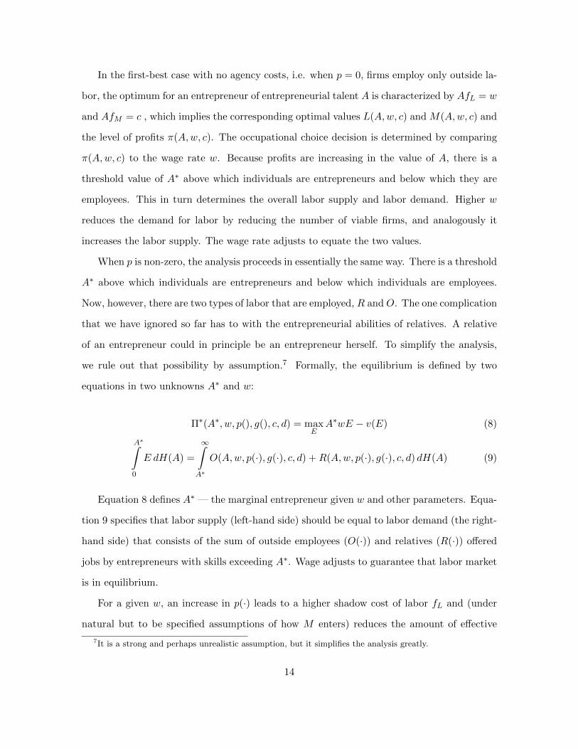
In the first-best case with no agency costs, i.e. when p = 0, firms employ only outside la-

bor, the optimum for an entrepreneur of entrepreneurial talent A is characterized by AfL = w

and AfM = c , which implies the corresponding optimal values L(A,w, c) and M(A,w, c) and

the level of profits π(A,w, c). The occupational choice decision is determined by comparing

π(A,w, c) to the wage rate w. Because profits are increasing in the value of A, there is a

threshold value of A∗ above which individuals are entrepreneurs and below which they are

employees. This in turn determines the overall labor supply and labor demand. Higher w

reduces the demand for labor by reducing the number of viable firms, and analogously it

increases the labor supply. The wage rate adjusts to equate the two values.

When p is non-zero, the analysis proceeds in essentially the same way. There is a threshold

A∗ above which individuals are entrepreneurs and below which individuals are employees.

Now, however, there are two types of labor that are employed, R and O. The one complication

that we have ignored so far has to with the entrepreneurial abilities of relatives. A relative

of an entrepreneur could in principle be an entrepreneur herself. To simplify the analysis,

we rule out that possibility by assumption.7 Formally, the equilibrium is defined by two

equations in two unknowns A∗ and w:

Π∗(A∗, w, p(), g(), c, d) = maxE

A∗wE − v(E) (8)

A∗ˆ

0

E dH(A) =

∞

A∗

O(A,w, p(·), g(·), c, d) +R(A,w, p(·), g(·), c, d) dH(A) (9)

Equation 8 defines A∗ — the marginal entrepreneur given w and other parameters. Equa-

tion 9 specifies that labor supply (left-hand side) should be equal to labor demand (the right-

hand side) that consists of the sum of outside employees (O(·)) and relatives (R(·)) offered

jobs by entrepreneurs with skills exceeding A∗. Wage adjusts to guarantee that labor market

is in equilibrium.

For a given w, an increase in p(·) leads to a higher shadow cost of labor fL and (under

natural but to be specified assumptions of how M enters) reduces the amount of effective

7It is a strong and perhaps unrealistic assumption, but it simplifies the analysis greatly.

14

labor hired, L = O+αR. For firms that continue to employ no relatives, the overall number

of employees then has to fall. For firms that do employ relatives, the effect on overall labor

O+αR and the effect on the number of employees O+R is not the same, but it is possible to

show that while the number of relatives employed increases, the number of overall employees

O +R has to fall. Naturally, an increase in p, holding other things constant, reduces profits

as well. Thus, given the wage, the number of entrepreneurs has to fall and the number of

employees has to increase. Given these shifts in supply and demand of labor, there is a further

adjustment: more individuals are willing to work for their relatives which acts to partially

mitigate the decline in labor and the decline in profits. The wage needs to adjust downwards

to establish an equilibrium.

3.2 Summary of the undistorted model

The baseline model contains many moving elements and in what follows we will consider

its substantial simplifications. Before proceeding with the analysis of tax policy, it is worth

noting a number of its properties and summarize the important elements.

First, the production technology allows for many different inputs:

1. entrepreneurial effort devoted to running the firm, E

2. entrepreneurial effort devoted to monitoring employees activity, F

3. overall labor employed L = O + αR

(a) that consists of outside employees O

(b) and related employees R

4. two additional inputs — M and N — that influence agency costs; absent taxation,

there is no qualitative difference between M and N , but in what follows we will allow

for differing observability assumptions about the two inputs: we will assume that M

may be observed by the tax authorities but N is not. In particular and previewing

later discussion, N is an avenue for tax evasion. In fact, one one special case of this

15

framework is when M and N are substitutes in production — F (·,M + N, ·) — and,

in the simplest case have the same cost c = d, but X(M,N) = X(N) so that N is

dominated by M absent additional considerations. In the presence of taxation though,

relying on unobservable N may turn out to be optimal. In that case, N can be thought

as precisely representing tax evasion with p(F )(O +´ R0 g(r))X(N) representing the

cost of tax evasion in the spirit of the cost-of-sheltering technology considered eg. by

Slemrod (2001). More generally, N may be mixing “real” and “avoidance” aspects.

Given all these inputs, the firm employs technology given by F (E,O + αR,M,N,A) −

p(F )(O +´g(r))X(M,N)) - this is a technology that has multiple inputs and is compli-

cated due to allowance for the agency costs but otherwise standard. Beyond that, the cost

of inputs is O, R, M and N is linear (with the cost of M and N given exogenously and the

cost of labor inputs determined in equilibrium), while the cost of inputs E and F stems from

disutility of effort by the entrepreneur v(E + F ).

All individuals vary by the level of their ability A. Ability for individuals who choose to

be entrepreneurs influences the productivity of a firm. For employees, the ability is standard

as in the Mirrlees framework, with A denoting the efficiency per hour of labor supply so that

the wage per hour that an individual with ability A receives is given by wA.

The economy is efficient given the values of parameters. Some of the parameters that

were already introduced can be thought of as reflecting policy or the quality of institutions.

For example, function g() reflects availability of relatives and hence the social fabric of the

society. Schedule p(·) reflects the importance of monitoring costs — possibly, in societies with

better contract enforcement p(·) is lower than otherwise. Also, prices of inputs may be to

some extent reflect institutions and policy. In particular, consider the case when M are visible

monetary inputs (bank accounts) while N is unreported cash. The value of d (and the extent

to which it exceeds c) may reflect government’s investment in the quality of the financial

sector — in this sense, this parameter can measure the value of attachment to the financial

sector that is key to the analysis of Gordon and Li (2009). We will consider comparative

statics with respect to these parameters but will not model their optimal setting. Instead, in

16

the next section we will clarify how to think about tax policy in the current context and, in

particular, we will focus on observability assumptions.

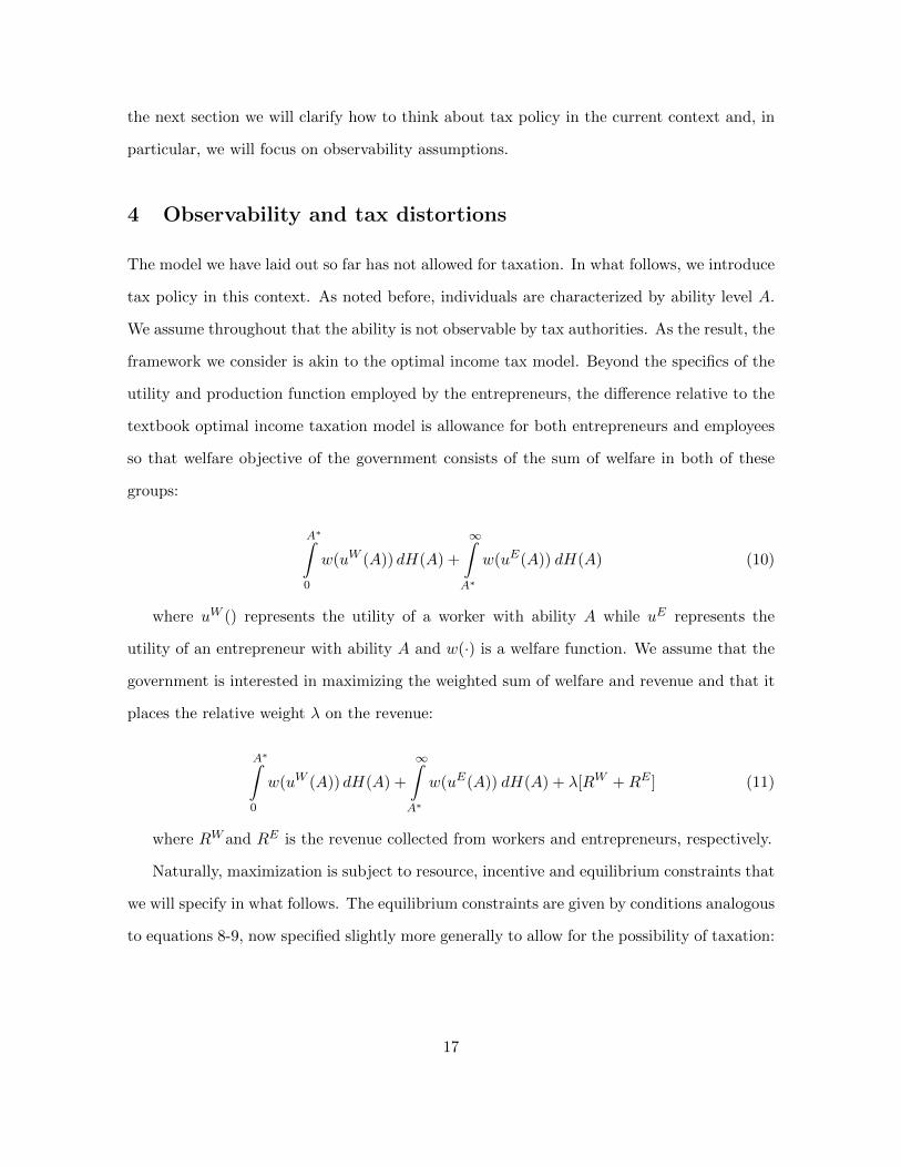
4 Observability and tax distortions

The model we have laid out so far has not allowed for taxation. In what follows, we introduce

tax policy in this context. As noted before, individuals are characterized by ability level A.

We assume throughout that the ability is not observable by tax authorities. As the result, the

framework we consider is akin to the optimal income tax model. Beyond the specifics of the

utility and production function employed by the entrepreneurs, the difference relative to the

textbook optimal income taxation model is allowance for both entrepreneurs and employees

so that welfare objective of the government consists of the sum of welfare in both of these

groups:

A∗ˆ

0

w(uW (A)) dH(A) +

∞

A∗

w(uE(A)) dH(A) (10)

where uW () represents the utility of a worker with ability A while uE represents the

utility of an entrepreneur with ability A and w(·) is a welfare function. We assume that the

government is interested in maximizing the weighted sum of welfare and revenue and that it

places the relative weight λ on the revenue:

A∗ˆ

0

w(uW (A)) dH(A) +

∞

A∗

w(uE(A)) dH(A) + λ[RW +RE ] (11)

where RW and RE is the revenue collected from workers and entrepreneurs, respectively.

Naturally, maximization is subject to resource, incentive and equilibrium constraints that

we will specify in what follows. The equilibrium constraints are given by conditions analogous

to equations 8-9, now specified slightly more generally to allow for the possibility of taxation:

17

uW (A∗) = uE(A∗) (12)A∗ˆ

0

E dH(A) =

∞

A∗

O +RdH(A) (13)

We assume that the government can tell apart entrepreneurs from employees so that

it will design separate tax schedules for the two groups, subject to the equilibrium and

revenue constraints. In particular, the two weak inequalities signified by equation 12 serve

as “participation” condition for being in either sector (or, formally, terminal/transversality

conditions for end-points of the two population present in either sector). The two sectors are

linked through the equilibrium conditions that in turn require values of A∗ and w to adjust.

We will characterize the optimal policy in each sector, for any value of w and A∗; with the

full optimum additionally corresponding to the specific values of w and A∗ that satisfy the

two equilibrium conditions.

We will pursue the standard optimal control approach to characterizing the optimal policy,

characterizing the optimal allocation first with the corresponding marginal tax rates implicitly

characterized. Beginning first with the (much simpler) employee sector and recalling that

the utility is simply given by C − v(E) or, equivalently C − v( yA

), the planner’s problem can

be set up in the standard way by leveraging the revelation principle. Government proposes

the schedule (u(A), c(A), y(A)) that satisfies u(A) = c(A)−v(y(A)A

), the incentive constraint

(envelope condition) u = − yA2 v

′ ( yA

). Correspondingly, the tax liability (contribution to the

overall revenue) is given by wy(A) − c(A). This is a standard optimal income tax Mirrlees

model with quasi-linear preferences (as consider by, for example, Weymark, 1987; Werning,

2007), complicated only by the fact that the equilibrium conditions potentially modify the

allocation at the top of the distribution (thereby shifting the whole corresponding tax schedule

up or down) and because the presence of an endogenous wage might (but do not have to) give

rise to a uniform adjustment of the whole tax schedule reflecting a potential redistributive

externality as in Naito (1999). This problem has built into it observability assumptions: it

18

is assumed that the government is able to observe income of employees. This assumption

can be reconsidered. For example, given the family structure, it might be interesting to

consider instead the situation where income of unrelated might be observed but income of

related employees is not or is observed only to a limited extent (e.g., the total payroll may

be observed or payments are only partially visible). This is left for the future analysis.

More interesting is the entrepreneurial sector. Here, it is helpful to write the allocation

as consisting of multiple schedules, some of which will be redundant and some of which will

correspond to additional constraints. To begin, recall the structure of production

π(E,F,O,R,M,N ;A) = F (E,O+αR,M,N ;A)−cM−dN−w(O+R)−p(F )(O+

R

0

g(r)dr)X(M,N)

The entrepreneur maximizes the utility u(C,E + F ) = C − v(E + F ) where

C = π(E,F,O,R,M,N ;A)− T (·)

where T is the tax liability with arguments reflecting observability assumptions. We will

assume that A cannot be observed and furthermore that effort (neither E nor F ) cannot be

observed either. As mentioned before, the parameter N was introduced with the sole purpose

of analyzing implications of its non-observability. We assume for now that the government

can observe M , R, O and output F (E,O + αR,M,N ;A).

Government proposes a path of utility, u(A), profits π(A), consumption C(A) and input

variables M(A), N(A), R(A), O(A), E(A) and F (A). Because E and A are not observable

(and so is N and F , but we want to be very flexible about how it enters), observing the level of

output does not in general allow for recovering the value of A. As the result, individuals may

misreport their type. The unobservable variables can be selected freely though — individuals

are not bound to select values of E, F and N that correspond to their reported type. Two of

these variables — E and N — influence tax liability only through their effect on output (which

19

is assumed to be observed) while F has no impact on any observable quantity. Denoting the

derivative of the tax schedule with respect to the level of output by TY , the unobservability

gives rise to the three first-order conditions that the planner has to respect:

FE(1− TY ) = v′(E + F ) (14)

p′(F )(O +

R

0

g(r) dr)X(M,N) = v′(E + F ) (15)

FN (1− TY ) = d+ p(F )(O +

R

0

g(r) dr)XN (M,N) (16)

These constraints involve the derivative of the unknown tax function. Equation 14 can

be used as the definition of this wedge and the last constraint may be modified to obtain

v′(E + F )

FE(E,F,O,R,M,N,A)=

d+ p(F )(O +R

0

g(r) dr)XN (M,N)

FN (E,F,O,R,M,N ;A)(17)

— now expressed in the primary form. Writing the constraint in this form is useful for an

additional reason. The left-hand side represents the tax wedge — 1− TY — while the right-

hand side reflects the trade-off between costs and benefits of modifying N . A potential policy

modification that manipulates the left-hand side (marginal tax rate on output) must involve

an adjustment of N to balance this condition. Hence, this condition is about responsiveness

of N to tax incentives and it will be a useful exercise for building the intuition to clarify it

further.

Finally, in the standard way, the revelation principle implies the incentive constraint

u = FA(E,F,O,R,M,N ;A) · (1− TY ) (18)

As before, this constraint involves the derivative of the unknown tax function and can be

rewritten as

20

u =FA(E,F,O,R,M,N ;A)

FE(E,F,O,R,M,N ;A)· v′(E + F ) (19)

Putting pieces together, government optimization is subject to the incentive constraint

19 and two non-observability constraints 15 and 17. Clearly, this is a complicated set of

constraints and it is useful to consider its simplified cases. A very useful special case is when

production function is given by

Assumption 1. Multiplicative technology given by F (AE,F,O,R,M,N).

In that case, the incentive constraint simplifies dramatically to

u =E

Av′(E + F ) (20)

or, with substitution of variables as Y = AE, to

u =Y

A2v′(Y

A+ F

)(21)

In this special case, the incentive constraint does not depend on variables other than

effort. This situation is akin to the weak-separability assumption underlying the celebrated

Atkinson and Stiglitz (1976) role that finds no role for commodity distortions. Here, the effect

of ability works its way on firm behavior through Y = AE so that, hypothetically, if Y was

observable, no other variable would contain useful information about productivity beyond

what is contained in Y . While Y itself is not observable, a monotone function of Y (output)

is, and by analogy one expects that there is no additional information about productivity from

observing inputs beyond what is embedded in output. We will show shortly that implications

are similar to the Atkinson-Stiglitz result.

The contribution of an individual with abilityA to the revenue collected from entrepreneurs

can be expressed as

RE = (π(A)− C(A))h(A) (22)

21

Finally, the equilibrium constraint 13 involves overall labor demand by entrepreneurs,

Z =´∞A∗ O +RdH(A) and the corresponding differential equation is simply

Z = (O +R)h(A) (23)

Thus, the objective of the government is given by formula 11 (with revenue from the

marginal individual spelled out as in 22) and is subject to the incentive constraint 19 (or,

under simplifying assumptions, constraint 21) as well as the non-observability constraints 15

and 17. Optimization is also subject to the equilibrium condition 13 that yields the law of

motion for the aggregate labor demand given by equation 23. There are additionally termi-

nal/initial conditions: the restriction on the value of A∗ (equation 12), the labor equilibrium

condition itself that translates in a restriction on the terminal value of Z and zero restriction

for the initial value of revenue. Beyond aggregate/equilibrium variables (RE , Z), optimiza-

tion is subject to a number of variables: u, π, C, and the choice variables of the individual

(with π and u explicitly defined in terms of other variables) with the explicit law of motion

for u alone stemming from the incentive constraint. While this may seem like a compli-

cated problem, it has very similar to the standard optimal income tax problem with multiple

goods, with non-observability and equilibrium constraints providing additional wrinkles and

the production function imposing structure.

In what follows, we ignore terminal/initial conditions that pin down the path of all vari-

ables and instead focus on marginal distortions that can be characterized without adding

these constraints. The objective and all the constraints have been expressed in terms of real

variables so that putting these together to apply the maximization principle, the correspond-

ing Hamiltonian may be written as

22

H =w(u) · h(A) + λ(π − C)h(A) + µu+ ψ · (O +R)h(A)

+ ρ · [C − v(F + E)− u]

+ ν ·

F (E,O + αR,M,N ;A)− cM − dN − w(O +R)− p(F )(O +

R

0

g(r)dr)X(M,N)− π

(24)

+ ηN ·

[d+ p(F )(O +

´ R0 g(r) dr)XN (M,N)

FN− v′(F + E)

FE

]

+ ηF ·

p′(F )(O +

R

0

g(r) dr)X(M,N)− v′(E + F )

Unless otherwise specified, for now we will pursue by ignoring the last constraint, which

amounts to assuming that p(F ) = p, i.e. that it is constant.

There are a few immediate simplifications. First-order conditions with respect to C and

π imply ρ = ν = λh(A) (recall that λ is the weight on government revenue) — this simply

corresponds to substituting away for C and π from the formulas that define them. Because

aggregate demand Z is not an argument to the Hamiltonian, ψ = 0 so that ψ is constant — it

is the multiplier on equilibrium labor market constraint. Whether this multiplier is non-zero

is an interesting question that we leave aside for now — it might be if distorting the relative

wages of employees and entrepreneurs is optimal as in the case considered by Naito (1999).

The only dynamic condition is the law of motion for µ — the multiplier on the incentive

constraint:

− µ =∂H∂u

= (w′(u)− λ)h(A) (25)

that simply reflects the trade-off between the two uses of resources: utility and revenue.

More interestingly, the first-order conditions with respect to the choice variables characterize

the structure of the optimal distortions. We will begin by briefly characterizing the first-order

23

condition corresponding to E. It is given by

µdu

dE− λh(A)v′(E + F ) + λFEh(A) + · · · = 0

The omitted terms on the right hand side correspond to the non-observability constraints.

It is instructive to consider the situation when they are not present (F and N are not part

of the problem or are observable). Then, the condition reduces to

v′(E + F )

FE− 1 =

µ

λh(A)FE

du

dE

The left-hand side is the distortion to the choice of E (the wedge that the planner imposes)

— the undistorted outcome is v′(E + F ) = FE . The whole formula is analogous to the basic

formula for the optimal income tax rate. The solution for µ may be directly derived by

straightforwardly integrating equation 25, λ is constant and known and h(A) is given. The

more complicated term dudE potentially depends on many inputs when the incentive constraint

is given by 19. Recall though that effort (or, derived from itY = AE) is not observable. We

did assume though that output can be observed. Hence, recalling the constraint 14, these

formulas define the optimal marginal tax rate imposed on the output level, TY :

TY = − µ

λh(A)FE

du

dE

In the special case corresponding to assumption 1 and the corresponding incentive con-

straint 21, the optimal wedge is given by

TY = 1−v′(YA + F )

AFY= −

µv′(YA + F )

λh(A)AFY

[1 +

v′′(YA + F )

v′(YA + F )· YA

]

The additively separable structure of the utility that would correspond to setting F = 0

(p(F ) = p) corresponds to a natural special case that has been extensively analyzed in the

literature on optimal income taxation. Assuming isoelastic structure of v(·) would yield

further simplifications.

24

To gain additional insight consider the first-order condition with respect to M , again

considering the case without the non-observability constraints :

µdu

dM+ λh(A)

FM − c− p(F )(O +

R

0

g(r) dr)XM

= 0 (26)

Again, as before consider the multiplicative case given by assumption 1. In that case,

dudM = 0 and the above first-order condition implies that the choice of M should not be

distorted. In the presence of taxation, the choice of M is given by

FM − c− p(F )(O +

R

0

g(r) dr)XM − TY · FM − TM = 0

and we have just established that TY 6= 0 so that setting TY · FM + TM = 0 requires

TM 6= 0. In particular, it easy to show that what is required is that the tax has the structure

of T

(F (·,M, ·)− cM − p(F )(O +

R

0

g(r) dr)X(M,N), ·

)where omitted arguments do not

depend on M . In other words, in this special case, the system should involve pure profit

taxation. An analogous argument will apply to any other input.

Remark 2. Suppose that assumption 1 is satisfied, non-observability constraints are not

present and the equilibrium conditions are not imposed. Then, the optimal tax system

for entrepreneurs involves a non-linear profit tax.

This is the analogue of the Atkinson-Stiglitz theorem in the optimal income tax case.

When inputs do not provide independent information about ability over an observable quan-

tity such as output, their relative prices should not be distorted. In particular, given produc-

tion structure, the lack of distortion requires relying on profit tax.

Conversely, when assumption 1 is not satisfied and dudM 6= 0, the optimal tax structure

should deviate from profit taxation and involve distortions to the relative price of M .

Note further that whether one should allow for full expensing of M does not depend on

whether all inputs are observable, as long as their corresponding non-observability constraints

are not affected by M — in such a case the first order condition 26 will not be affected and

25

the whole argument goes through.

Now consider the case of an unobservable input N and a relaxed problem where non-

observability condition was not imposed. The same argument as in the case of M goes

through — the first-order condition for N should not be distorted and the optimal tax should

allowing for expensing of this input. This is however no longer feasible because N cannot be

observed or, put differently, such a requirement violates the non-observability constraint 17.

The non-observability constraint does not correspond to undistorted first-order condition for

N : because output is taxed, the marginal benefit of N is affected by the tax but because N

is not observed there is no corresponding mechanism for offsetting that distortion. Hence,

the non-observability constraint is binding and implications of non-observability of N are

non-trivial.

To begin analyzing those implications, reconsider the choice of the effort, now accounting

for implications of non-observability of input N . The first order condition for effort is now

µdu

dE−λh(A)v′(E+F )+λFEh(A)−ηN

∂

∂E

{d+ p(F )(O +

´ R0 g(r) dr)XN (M,N)

FN− v′(F + E)

FE

}= 0

yielding the formula for the optimal wedge

TY = 1− v′(E + F )

FE=

− µ

λh(A)FE

du

dE+

ηNλh(A)FE

∂

∂E

{d+ p(F )(O +

´ R0 g(r) dr)XN (M,N)

FN− v′(F + E)

FE

}

The optimal profit tax rate is affected by the presence of unobservable inputs. The addi-

tional term is additive and reflects the effect on the non-observability constraint: modifying

taxation of output affects the optimal value of N — the strength (elasticity) of this effect is

reflected by the effect of E on the non-observability constraint (the last term) and is weighted

by the multiplier on that constraint ηN . One useful case for seeing the intuition here is to con-

26

sider the special case when the production function is additively separable between N and E.

Then, the last term reduces to − ηNλh(A)FE

∂∂E

{v′(F+E)FE

}and recalling that 1− TY = v′(F+E)

FE,

the very last term simply reflects the marginal tax rate adjustment implied by a change in

effort that will stimulate an adjustment in N . How important that adjustment is depends on

the magnitude of the multiplier ηN . Its value can be derived from the first-order condition

for N that yields

µdu

dN+ λh(A)

FN − d− p(F )(O +

R

0

g(r) dr)XN

+

ηN∂

∂N

{d+ p(F )(O +

´ R0 g(r) dr)XN (M,N)

FN− v′(F + E)

FE

}= 0 (27)

Substituting from the 17 and limiting attention to the separable case guaranteed by

assumption 1, the multiplier becomes

ηN = −λh(A)·(

1− v′

FE

)FN ·

{∂

∂N

{d+ p(F )(O +

´ R0 g(r) dr)XN (M,N)

FN− v′(F + E)

FE

}}−1

Two points are worth pointing out. First, the multiplier is zero when 1− v′

FE= 0 , that is

when there is no tax distortion. This is very intuitive: non-observability of N is not an issue

when it has no tax implications. Second, the last term is closely related to the elasticity of N

with respect to the tax rate (to be shown). One way to see it is to consider the case when E

and N enter the production function in a separable fashion so that FE does not depend on

N . Then, only the first term in the curly brackets — the ratio of marginal cost and benefits

— remains. The whole term measures how strongly that ratio reacts to changes in N which

is equivalent to asking how big of a response in N is expected in response to a change in tax

incentives (ie. v′

FE). More generally, a change in N may itself influence the magnitude of the

tax wedge which is accounted for by the presence of v′

FEin this formula.

27

Our analysis up to this point clarifies the structure of the model and its relationship to

the more standard optimal income tax problem. First, assumption 1 plays the role akin

to the weak separability assumption in the Atkinson and Stiglitz (1976) world. Under that

assumption and absent additional complications such as non-observability or binding equilib-

rium constraints, the optimal tax structure involves a tax on profits with deductions for all

inputs. In particular, there is no reason for distorting the choice between inputs, similarly as

in the A-S context there is no reason to impose commodity taxes once income may be taxed.

Relaxing this assumption provides a reason for taxing or subsidizing particular inputs, to the

extent that they interact with the incentive constraints.

Second, adding non-observability of some inputs modifies these conclusions in some ways.

It leads to the adjustment of the tax on profits to reflect the impact of this tax on hidden

activity and it does so in relationship to the strength of the response of the hidden activity. Its

interaction with inputs depends on whether a particular input affects the non-observability

constraint. In our case, whether the conclusion that M should be fully expensed is modified

depends on whether M affects the constraint 17. It may do so when M is a production

substitute or complement to either hidden input (FMN 6= 0), effort (FEM 6= 0) or when the

agency costs interact (XMN 6= 0). Put differently, what matters is whether that particular

input influences the extent of unobservable action (in the extreme case, tax evasion).

The inputs of most interest in our context are of course family and outside labor supply.

Qualitatively, many features of our discussion so far apply. If they are observable and they can

be expensed, they should be because this is what is required for implementing (optimal under

assumption 1) profit taxation. When there are no non-observable inputs except for effort,

this conclusion applies. However, at the heart of considering the problem of taxing family

firms is non-observability. The agency costs are unlikely to be observed and the mechanism

for that in the model is their dependence on N — without N influencing agency costs, they

could be recovered based on (assumed observable) values of M , O and R.

We proceed by again limiting the attention to the separable case guaranteed by assump-

tion 1. We further assume a very special form of the production function: F (EA,L,M,N) =

28

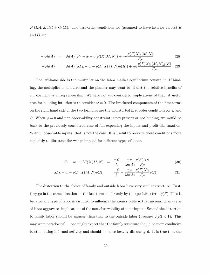
F1(EA,M,N) + G2(L). The first-order conditions for (assumed to have interior values) R

and O are

− ψh(A) = λh(A) (FL − w − p(F )X(M,N)) + ηNp(F )XN (M,N)

FN(28)

−ψh(A) = λh(A) (αFL − w − p(F )X(M,N)g(R)) + ηNp(F )XN (M,N)g(R)

FN(29)

The left-hand side is the multiplier on the labor market equilibrium constraint. If bind-

ing, the multiplier is non-zero and the planner may want to distort the relative benefits of

employment vs entrepreneurship. We have not yet considered implications of that. A useful

case for building intuition is to consider ψ = 0. The bracketed components of the first terms

on the right hand side of the two formulas are the undistorted first order conditions for L and

R. When ψ = 0 and non-observability constraint is not present or not binding, we would be

back to the previously considered case of full expensing the inputs and profit-like taxation.

With unobservable inputs, that is not the case. It is useful to re-write these conditions more

explicitly to illustrate the wedge implied for different types of labor.

FL − w − p(F )X(M,N) =−ψλ− ηNλh(A)

p(F )XN

FN(30)

αFL − w − p(F )X(M,N)g(R) =−ψλ− ηNλh(A)

p(F )XN

FNg(R) (31)

The distortion to the choice of family and outside labor have very similar structure. First,

they go in the same direction — the last terms differ only by the (positive) term g(R). This is

because any type of labor is assumed to influence the agency costs so that increasing any type

of labor aggravates implications of the non-observability of some inputs. Second the distortion

to family labor should be smaller than that to the outside labor (because g(R) < 1). This

may seem paradoxical — one might expect that the family structure should be more conducive

to stimulating informal activity and should be more heavily discouraged. It is true that the

29

family structure makes the cost of increasing X(M,N) (and, therefore, changing the hidden

activity) lower than otherwise. However, what this framework highlights is that this implies

that unobservable agency costs are then lower holding other things constant. With lower

agency costs, the optimal tax structure resembles more closely profit taxation that would be

optimal if there were no hidden actions.

The discussion so far relied on the assumption that F (EA,L,M,N) = F1(EA,M,N) +

G2(L). Relaxing that assumption and considering instead F (EA,L,M,N) would modify

the first-order conditions 30-31 to account for the effect of changes in O and R on FE and

FN present in constraint 17. These effects are closely related because the two types of

labor influence marginal product of E and N jointly as labor L = O + αR. As the result,

the distortion stemming from these effects will be multiplier by the factor α in the case of

employing relatives relative to the outside labor. More explicitly, the effect of a change in L

(the argument of production function) on the constraint 17 is given by

∂

∂L

{d+ p(F )(O +

´ R0 g(r) dr)XN (M,N)

FN− v′(F + E)

FE

}=

−FNLFN

d+ p(F )(O +´ R0 g(r) dr)XN (M,N)

FN+FELFE

v′(F + E)

FE=

(FELFN− FNL

FE

)v′(F + E)

FE

where the last equality applies the constraint 17 itself to substitute and simplify. The case

of FEL = FNL = 0 that we considered before makes this term zero and also a weaker case of

the weakly separable production function F (g(AE,N), L) would do so. The mechanism at

play here has to do with the interaction of labor with effort vs unobservable inputs. In general,

labor may interact with both but implications depend on which one is affected more strongly.

Again, it is helpful to recall the meaning of non-observability constraint 17. A change in

labor will encourage/discourage hidden activity N depending on the sign of FNL but it will

also simultaneously affect the incentives for effort — profit taxation, v′

FE— depending on

FEL. Which of these effects is stronger matters so that even if hidden action (e.g., cash

30

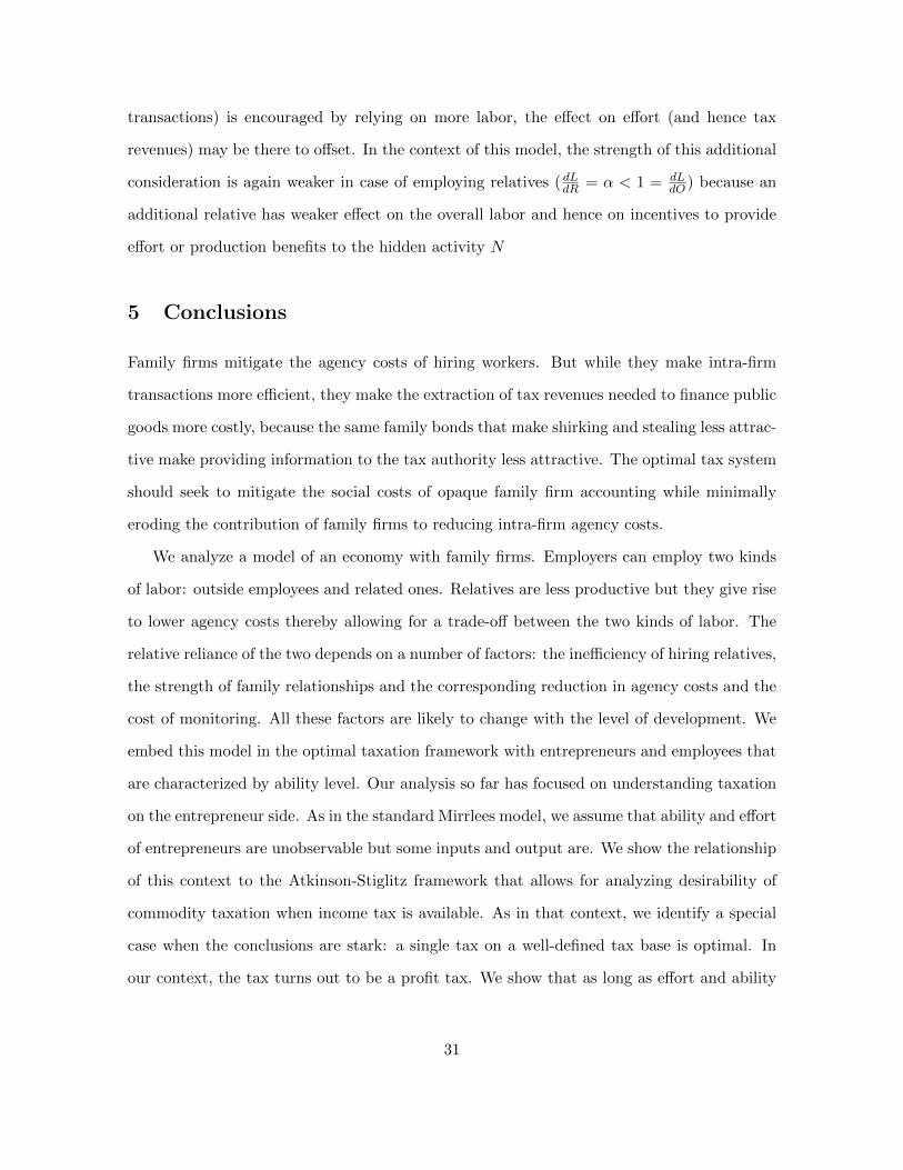
transactions) is encouraged by relying on more labor, the effect on effort (and hence tax

revenues) may be there to offset. In the context of this model, the strength of this additional

consideration is again weaker in case of employing relatives ( dLdR = α < 1 = dLdO ) because an

additional relative has weaker effect on the overall labor and hence on incentives to provide

effort or production benefits to the hidden activity N

5 Conclusions

Family firms mitigate the agency costs of hiring workers. But while they make intra-firm

transactions more efficient, they make the extraction of tax revenues needed to finance public

goods more costly, because the same family bonds that make shirking and stealing less attrac-

tive make providing information to the tax authority less attractive. The optimal tax system

should seek to mitigate the social costs of opaque family firm accounting while minimally

eroding the contribution of family firms to reducing intra-firm agency costs.

We analyze a model of an economy with family firms. Employers can employ two kinds

of labor: outside employees and related ones. Relatives are less productive but they give rise

to lower agency costs thereby allowing for a trade-off between the two kinds of labor. The

relative reliance of the two depends on a number of factors: the inefficiency of hiring relatives,

the strength of family relationships and the corresponding reduction in agency costs and the

cost of monitoring. All these factors are likely to change with the level of development. We

embed this model in the optimal taxation framework with entrepreneurs and employees that

are characterized by ability level. Our analysis so far has focused on understanding taxation

on the entrepreneur side. As in the standard Mirrlees model, we assume that ability and effort

of entrepreneurs are unobservable but some inputs and output are. We show the relationship

of this context to the Atkinson-Stiglitz framework that allows for analyzing desirability of

commodity taxation when income tax is available. As in that context, we identify a special

case when the conclusions are stark: a single tax on a well-defined tax base is optimal. In

our context, the tax turns out to be a profit tax. We show that as long as effort and ability

31

are separable from other inputs, the optimal policy should feature profit taxation with full

expensing of the cost of all inputs. While this is optimum if feasible to implement, our

interest in analyzing firms built on trust is precisely in considering cases when pure profit tax

is infeasible. To do so, we allow for hidden actions — holding money in cash for example —

that are made cheaper by relying on relatives. Because such behavior is not observed by tax

authorities, it is the mechanism for introducing tax avoidance/evasion in the model. Taxation

of profits is naturally affected by the responsiveness of hidden actions to the tax. Distortions

to relative prices of inputs arise to the extent that such inputs interact with hidden actions and

reflect such impact. Interestingly though, implications of such hidden actions for treatment

of family firms are somewhat unexpected. To the extent that intensity of employing labor in

general affects propensity to engage in behavior unobservable by tax authorities, all types of

labor should be distorted — both formal and informal. If productive benefits of holding cash

or engaging in other unobservable behavior vary depending on whether one employs relatives

or outside labor, this conclusion may be more nuanced but it is outside of our current model.

On the other hand, relying on relatives makes unobservable agency costs smaller and hence

the departure from profit taxation weaker than otherwise. This mechanism implies that the

distortion to employing relatives should be weaker than the distortion to employing outside

labor.

Our analysis of the model focused on providing intuition for the forces at play and we

plan to build on it to provide a more careful exposition of our results. In particular, we

have not yet analyzed implications of labor market equilibrium, the possibility of the overall

distortions to the entrepreneur-employee choices and implications of various corner solutions

such as firms that solely employ labor or that solely employ relatives. We also have not yet

considered the interaction of the employee and employer side of taxation. Further discussion

of the comparative statics is very interesting as well. There are many other extensions

that are worth considering. Our model assumes that authorities can distinguish employing

relative from employing outside labor. This is not necessarily realistic and weakening this

assumption would be of interest. As is standard in the optimal income tax literature, we

32

focus on a one-dimensional context — ability differences. This makes the task of the social

planner who wants to account for unobservable behavior easier than otherwise. Allowing for

heterogeneity in agency costs is a natural extension.

33

References

Atkinson, Anthony B. and Joseph E. Stiglitz, “The Design of Tax Structure: Direct

versus Indirect Taxation,” Journal of Public Economics, July-August 1976, 6 (1-2), 55–75.

Ben-Porath, Yoram, “The F-Connection: Families, Friends, and Firms and the Organiza-

tion of Exchange,” Population and Development Review, 1980, 6 (1), 1–30.

Bertrand, Marianne and Antoinette Schoar, “The Role of Family in Family Firms,”

Journal of Economic Perspectives, 2006, 20 (2), 73–96.

Besley, Timothy and Torsten Persson, “The Origins of State Capacity: Property Rights,

Taxation, and Politics.,” American Economic Review, 2009, 99 (4), 1218–1244.

Bhattacharya, Utpal and B. Ravikumar, “Capital Markets and the Evolution of Family

Businesses,” Journal of Business, 2001, 74 (2), 187–219.

and , “From Cronies to Professionals: The Evolution of Family Firms,” in E. Klein,

ed., Capital Formation, Governance and Banking, Nova Science Publishers, 2004.

Bloom, Nicholas and John Van Reenen, “Measuring and Explaining Management Prac-

tices Across Firms and Countries,” Quarterly Journal of Economics, 2007, 122 (4), 1351–

1408.

Burkart, Mike, Fausto Panunzi, and Andrei Shleifer, “Family Firms,” 2003, 58 (5),

2167–2201.

Christensen, Kevin, Robert Cline, and Tom Neubig, “Total Corporate Taxation:

’Hidden,’ Above-the-Line, Non-income Taxes,” National Tax Journal, 2001, 54 (3), 495–

506.

Claessens, Stijn, Simeon Djankov, and Larry H. P. Lang, “The Separation of Own-

ership and Control in East Asian Corporations,” Journal of Financial Economics, 2000,

58 (1-2), 81–112.

34

Desai, Mihir A., Alexander Dyck, and Luigi Zingales, “Theft and Taxes,” Journal of

Financial Economics, 2007, 84 (3), 591–623.

and Dhammika Dharmapala, “Corporate Tax Avoidance and High-Powered Incen-

tives,” Journal of Financial Economics, 2006, 79 (1), 145–179.

Diamond, Peter A. and James A. Mirrlees, “Optimal Taxation and Public Production,”

American Economic Review, March-June 1971, 61 (1,3), 8–27,261–78.

Fisman, Raymond, “Estimating the Value of Political Connections,” American Economic

Review, 2001, 91 (4), 1095–1102.

Gordon, Roger and Wei Li, “Tax Structures in Developing Countries: Many Puzzles and

a Possible Explanation,” Journal of Public Economics, August 2009, 93 (7-8), 855–866.

Jackson, C. Kirabo and Henry S. Schneider, “Do Social Connections Reduce Moral

Hazard? Evidence from the New York City Taxi Industry,” American Economic Journal:

Applied Economics, jul 2011, 3 (3), 244–67.

Kleven, Henrik J., Claus Thustrup Kreiner, and Emmanuel Saez, “Why Can Mod-

ern Governments Tax So Much? An Agency Model of Firms as Fiscal Intermediaries,”

Working Paper 15218, National Bureau of Economic Research August 2009.

Kopczuk, Wojciech and Joel Slemrod, “Putting Firms into Optimal Tax Theory,” Amer-

ican Economic Review Papers and Proceedings, May 2006, 96 (2), 130–134.

La Porta, Rafael, Florencio Lopez de Silanes, Andrei Shleifer, and Robert W.

Vishny, “Trust in Large Organizations,” American Economic Review Papers and Proceed-

ings, 1997, 87 (2), 333–338.

Lucas, Robert E. Jr., “On the Size Distribution of Business Firms,” Bell Journal of

Economics, 1978, 9 (2), 508–523.

35

Murphy, Kevin M., Andrei Shleifer, and Robert W. Vishny, “The Allocation of

Talent: Implications for Growth,” Quarterly Journal of Economics, 1991, 106 (2), 503–

530.

Naito, Hisahiro, “Re-examination of Uniform Commodity Taxes under a Non-Linear Tax

System and Its Implication for Production Efficiency,” Journal of Public Economics, Febru-

ary 1999, 71 (2), 165–188.

Perez-Gonzalez, Francisco, “Inherited Control and Firm Performance,” American Eco-

nomic Review, 2006, 96 (5), 1559–1588.

Rebitzer, James B and Lowell J. Taylor, “Extrinsic Rewards and Intrinsic Motives:

Standard and Behavioral Approaches to Agency and Labor Markets,” in “Handbook of

Labor Economics” 2010. forthcoming.

Schulze, William S., Michael H. Lubatkin, and Richard N. Dino, “Altruism, Agency,

and the Competitiveness of Family Firms,” Managerial and Decision Economics, 2002, 23

(4-5), 247–259.

Slemrod, Joel, “A General Model of the Behavioral Response to Taxation,” International

Tax and Public Finance, March 2001, 8 (2), 119–28.

Villalonga, Belen and Raphael Amit, “How do family ownership, control and manage-

ment affect firm value?,” Journal of Financial Economics, 2006, 80 (2), 385–417.

Werning, Ivan, “Pareto Efficient Income Taxation,” April 2007. MIT, mimeo, http://

econ-www.mit.edu/files/1281.

Weymark, John A., “Comparative Statics Properties of Optimal Nonlinear Income Taxes,”

Econometrica, September 1987, 55 (5), 1165–1185.

Yitzhaki, Shlomo, “Cost-Benefit Analysis of Presumptive Taxation.,” FinanzArchiv, 2007,

63 (3), 311–326.

36

Chen, Shaping, Xia Chen, Qiang Cheng, and Terry Shevlin, “Are Family Firms

More Tax Aggressive than Non-Family Firms?” Working Paper, November 2008.

Chrisman, James J., Jess H. Chua, and Pramodita Sharma, “Current Trends and

Future Directions in Family Business Management Studies: Toward a Theory of the family

Firm.” http://usasbe.org/knowledge/whitepapers/chrisman2003.pdf, 2003.

Dharmapala, Dhammika, Joel Slemrod, and John D. Wilson, “Tax Policy and the

Missing Middle: Optimal Tax Remittance with Firm-Level Administrative Costs.” University

of Michigan working paper, 2009.

International Tax Dialogue (with input from the staff of the International Monetary

Fund, Inter-American Development Bank, OECD, and the World Bank), Taxation of Small

and Medium Enterprises. Background paper for the International Tax Dialogue Conference,

Buenos Aires. October 2007.

Meade, James E., The Structure and Reform of Direct Taxation. Report of a Committee

chaired by Professor J.E. Meade. London: Institute for Fiscal Studies and George Allen &

Unwin, 1978

Morck, Randall, David A. Stangeland, and Bernard Yeung, “Inherited Wealth, Cor-

porate Control, and Economic Growth: The Canadian Disease.” In Concentrated Corpo-

rate Ownership. National Bureau of Economic Research Conference Volume. University of

Chicago Press, Chicago, IL, 2000.

Shaw, Jonathan, Joel Slemrod, and John Whiting, “Administration and Compliance,”

in Institute of Fiscal Studies (ed.), Dimensions of Tax Design: The Mirrlees Review, Oxford

University Press, Forthcoming.

37