tax and growth in a developing country the case of brazil ... · 5 . words. in this time period we...

Tax and Growth in a Developing Country: The Case of Brazil

Adolfo Sachsida1

Mario Jorge Cardoso de Mendonca2

Tito B. Moreira3

Abstract: This paper use Brazilian quarterly data, from the period Jan/2002 to June/2015, to estimate the impact of taxes over GDP per capita. The econometric results show a negative and statistically significant impact of the overall tax burden over per capita GDP. In average, an increase of 1 percent in the overall tax burden decreases GDP per capita by 0.3 percent. This result is very similar in magnitude with those presented by Heady et al. (2011). Furthermore, additional econometric results pointed out that a revenue neutral fiscal policy which changes the tax structure toward consumption taxes and personal income taxes would improve economic growth. Besides that, we strongly recommend against both taxes over the capital stock (mainly the recurrent ones) and the corporate income taxes.

Key-words: tax, economic growth, fiscal policy prescription.

JEL: E62, E69, H20.

1. Introduction

There is a considerable debate over the relation between taxes and economics

performance. Recently, Heady et al. (2011) elaborated a ranking of taxes stating that

changing the tax mix in direction of more consumption taxes (and away from corporate

income tax) would improve economic performance.

We follow the idea presented in Heady et al. (2011) and estimated a tax ranking

for a developing country (Brazil). This paper contributes to the literature applying the

1 Institute for Applied Economic Research. Email: [email protected]. Adolfo Sachsida acknowledge the research grant from CNPQ. We acknowledge the comments from University of Kent macroeconomic seminar participants. 2 Institute for Applied Economic Research. Email: [email protected] 3 Técnico do TCU.

methodology developed by Heady et al. (2011) to a single country. Instead of a panel

data technique this paper makes use of a time series approach to verify the impact of

taxes over the Brazilian GDP per capita.

The econometric results show a negative and statistically significant impact of

the overall tax burden over per capita GDP. In average, an increase of 1 percent in the

overall tax burden decreases GDP per capita by 0.3 percent. This result is very similar

in magnitude with those presented by Heady et al. (2011). Furthermore, our policy

prescription is very similar of that presented by Heady et al. (2011), that is, a revenue

neutral fiscal policy which changes the mix of tax burden toward consumption taxes and

away from corporate taxes has the potential to improve the economic performance.

Besides this introduction, section 2 presents the dataset and provides additional

information about the Brazilian tax system, section 3 introduce the econometric results,

section 4 explores the channel between tax burden and economic growth. Section 5

concludes the paper.

2. The Dataset

There are not a lot of doubts to claim that Brazil faces one of the worst tax

systems in the whole world. In February of 2016 Brazil counts 92 different kinds of

taxes4, and the government is struggling for the Congressional approval of another two

(a tax over big fortunes and a financial transaction tax over banking accounts). Not just

that there are too many taxes in Brazil, but their legislation suffers an incredible number

of changes in short time periods. For example, in the year of 2015 occur 27 major

changes in the tax legislation5.

In a study about changes in the Brazilian Constitution and in the tax system,

Amaral, Olenike, and Amaral (2013) showed that in 25 years Brazil experimented 15

tax reforms, besides that it were created several different types of taxes and

contributions, and almost all taxes were increased. They conclude that, in 25 years,

Brazil creates 309,147 new tax norms (29,939 by federal government, 93,062 by state

governments, and 186,146 by local governments), in average each norm has 3,000

4 http://www.portaltributario.com.br/tributos.htm 5 https://www.lsconcursos.com.br/principais-alteracoes-na-legislacao-tributaria-em-2015-d112.html

words. In this time period we had 31 new tax norms per day in Brazil. In October of

2013 the Brazilian tax system was composed by 262,705 articles (artigos), 612,103

paragraphs (paragrafos), 1,957,154 incises (incisos), and 257,451 aligns (alineas).

Assuming that a single firm does not make business outside the border of the state

which it is located, this firm would have to complain with an astonishing 3,512 tax

norms.

Messias (2013) presents some numbers about the litigious related to taxes in

Brazil. A lower bound estimation suggest that, in the year of 2013, there were US$ 330

billion related to litigious in taxes, or something around 15% of the Brazilian GDP. Just

to give an idea of this amount, the same value for the US economy was around 0.2% of

their GDP. In Brazil there are 16 tax suits for each 10,000 inhabitants. It is a much

higher number than in United States (1 for each 10,000 inhabitants), Canada (2 for each

10,000 inhabitants), United Kingdom (9 for each 10,000 inhabitants), or Swedish (13

for each 10,000 inhabitants).

According to the 2015 edition of Doing Business, a World Bank report which

measure business regulations for local firms around the world, in Brazil a medium size

company waste 2,600 hours per year with tax bureaucracy. Catar and Arab Emirates are

the fastest countries in this measure, with companies located there spending just 41

hours per year with tax bureaucracy. Developed countries around the world as United

Kingdom (110 hours per year), France (137 hours per year), United States (175 hours

per year), and Germany (218 hours per year) have a much faster way to deal with the

tax bureaucracy than Brazil. And even other developing countries in the world as

Mexico (334 hours per year), and Argentina (405 hours per year) performs better than

Brazil. After Brazil, the second worst country in the sample is Bolivia where companies

spend 1,025 hours with tax bureaucracy. That is, Brazil is almost three times slower

than the second worst country in its ability to deal with the bureaucracy of taxes.

It is very clear that the Brazilian tax system is confused, expensive, and

decreases both the competitiveness of the Brazilian companies and the productivity of

the economy. A tax reform is in much need, but to do that it is fundamental to have a

better idea of the impact of taxes over the economic growth.

This paper use Brazilian quarterly data, from the period Jan/2002 to June/2015,

to estimate the impact of taxes over GDP per capita. After that we are able to elaborate a

tax growth ranking suggesting the better mix of taxes to improve Brazilian economic

growth rate. Table A describes each variable adopted in this study.

Table A: Description of the variables#

Baseline Model

Real GDP per capita Quarterly real GDP per capita data. Build

from information available at Brazilian

Institute of Geography and Statistics

(IBGE).

Physical Capital Stock (k) This time series was build from

information collected in IPEADATA 6

(www.ipeadata.gov.br)7.

Physical Capital Stock per economically

active population (Kpea)

Refers to the physical capital stock

divided by the size of the population

classified as economically active8.

Human Capital Stock (h) Refers to the average years of schooling

of the population over 25 years old

Human Capital Stock (h2) Refers to the percentage of illiteracy

among individuals older than 15 years old.

Data from IPEADATA.

Population (pop) Refers to the size of the Brazilian

population. Build from information

available at Brazilian Institute of

Geography and Statistics (IBGE).

6 IPEADATA is an initiative of the Institute for Applied Economic Research (IPEA) to collect and make available in one site several socio-economic time series data for the Brazilian economy. 7 More information about the construction of the physical capital time series can be obtained in Morandi, L.; Reis, E. J. (2004). After the construction I compare it with another capital stock series, kindly provided by Roberto Ellery Jr. The correlation between them is 0.93. 8 Population economically active is the size of the population which satisfies two criteria: a) are working or looking for jobs; and b) are older than 15 years old.

Population Economically Active (pea) Refers to the size of the Brazilian

economically active population. Build

from information available at IPEADATA

(refers to 6 Brazilian metropolitan areas).

Overall Tax Burden (Total tax revenue /

GDP)

This time series was build following the

methodology suggested by Orair, Gobetti,

Leal, and Silva (2013) 9 and relies in

Brazilian official data.

Tax Structure Variables*

1) Income Tax Taxes related to income

1.1) Personal Income Tax Taxes related to personal income

1.2) Corporate Income Tax Taxes related to corporate income

2) Consumption Tax Taxes related to consumption and

production

3) Physical Capital Tax Taxes related to Physical Capital

3.1) Recurrent Tax on Properties Recurrent taxes on physical capital

3.2) Non-Recurrent Tax on Properties Non-Recurrent taxes on physical capital #: Two other variables were included in the regressions to verify the robustness of the results. Their inclusion does not change qualitatively the results of taxes over growth. These variables refers to a measure of openness of the Brazilian economy (as it can have impact on growth), and a measure of fiscal imbalances (since it can be related to the fiscal policy). Trade openness is measured as the ratio of imports to GDP; and the debt to GDP ratio is measured by the size of the Brazilian gross debt divided by GDP. Again, the inclusion of these variables does not have a qualitative impact on the results. *: the annex presents a Table showing where each tax is allocated between income, consumption or physical capital tax.

A brief overview of the Brazilian tax mix can be seen in Table B bellow. As

can be seen during the period Brazilian tax system relies a lot on consumption taxes

(75.2 percent of the taxes revenue come from this source), followed by income taxes

and taxes over capital stock or wealth (mainly the recurrent ones). Furthermore, we can

infer that this tax mix was constant over the period of our analysis.

Table B: Brief Overview of the Brazilian Tax Structure, percentage of each tax in

relation to the overall tax burden.

9 Rodrigo Orair kindly provided us with the update data until June/2015.

Tax Structure Average Maximum Minimum Std. Deviation

Personal Income Tax 10.8% 14.32% 8.63% 1.32%

Corporate Income Tax 9.9% 13.29% 6.49% 1.61%

Consumption Tax 75.2% 80.37% 68.77% 3.04%

Non-Recurrent Tax on Properties 0.6% 1.00% 0.35% 0.17%

Recurrent Tax on Properties 3.4% 7.12% 1.51% 1.92%

3. Econometric Results

In this section we analyze the effects of taxes over economic growth in the

Brazilian economy using quarterly data from the period Jan/2002 to June/2015. The

econometric strategy to verify the impact of the tax mix over growth will closely follow

Heady, Johansson, Arnold, Brys and Vartia (2009). The major difference is that in this

paper we will use time series techniques to check the tax mix effect over a specific

country, while Heady at all (2009) adopt panel data techniques in a set of OECD

countries.

Let us begin with a simple estimation of the impact of the overall tax burden

over the Brazilian economic growth. Table 1 presents this result. The physical and

human capital and the population are major sources for growth in the economic

textbooks. In Table 1 we present two different proxies for each one of these variables.

The effect of physical capital over growth is positive in all four regressions (and

statistically significant in three of them). The effect of human capital over growth is

positive and significant in three specifications (and statistically insignificant in the other

one). As soon as there are a lot of critics about how to measure human and physical

capital, we will not detail our analysis here. The idea of this paper is to verify the impact

of taxes over growth, and in line with it we can infer about a negative impact of the

overall tax burden over real GDP per capita. Column (1) of Table 1 shows that an

increase of 1 percent in the overall tax burden decreases real GDP per capita by 0.3

percent, and similar results are presented in the other columns. The four columns in

Table 1 present similar qualitative results about the negative, and statistically

significant, effect of the overall tax burden over per capita GDP. This reinforces and

gives more confidence to the negative effect of taxes over growth showing the

robustness of the tax results.

Table 1: The effect of the Overall Tax Burden over real GDP per capita#

Dependent variable: Ln of real GDP per capita

(1) (2) (3) (4)

Baseline Model Ln of Physical Capital (k)

2.46*** (.539)

1.42*** (.413)

Ln of Human Capital (average years of schooling)

-0.58 (.773)

Ln of Population (population)

1.01 (.731)

-0.18 (.588)

Control Variable Ln of the Overall Tax Burden (total revenues / GDP)

-0.32*** (.107)

-0.33*** (.103)

-0.38*** (.122)

-0.33*** (.103)

Other proxies Ln of per worker Physical Capital (kpea)

0.75 (.459)

1.42*** (.413)

Ln of Human Capital (illiteracy rate of population over 15 years old)

-0.52*** (.176)

-1.35*** (.223)

-0.52*** (.176)

Ln of Economically Active Population (pea)

0.12 (.433)

1.55*** (.343)

Constant -82.01*** (24.19)

-34.34*** (9.38)

-34.34*** (9.38)

Observations 54 54 54 54 F( 4, 49) =

211.87 F( 4, 49) = 246.38

F( 4, 49) = 170.79

F( 4, 49) = 246.38

Adj R-squared = 0.940




#: Standard errors are in brackets. *: significant at 10 % level; ** at 5% level; *** at 1 % level. The inclusion of lags does not change qualitatively the results. The inclusion of other variables as trade openness, a trend variable, and the debt ratio to GDP do not change qualitatively the results.

In the next step, let’s follow Heady at all (2009) and change our estimative

from level variables to first differences. The idea is that we can replicate a long run

pattern by a short run relationship with an error correction term. Additionally we can

include other control variables in the regression to check the robustness of the

econometric findings.

Table 2 verifies the effect of changes in the overall tax burden over growth

(growth rate of real GDP per capita). Because our human capital proxies are in annual

basis, we include its fourth difference to verify if results would change. Again, the tax

results are robust to it. In all the specifications we find a negative and statistically

significant effect of the overall tax burden over growth, ranging from -0.12 to -0.23.

That is, a 1 percent increase in the overall tax burden would decrease growth by a value

between 0.12 and 0.23 percent. This result is robust to a wide range of different

specifications.

Table 2: The effect of Changes in the Overall Tax Burden over Growth#

Dependent variable: growth rate of real GDP per capita

(1) (2) (3) (4)

Baseline Model ΔLn of Physical Capital

0.49 (.581)

1.84** (.880)

ΔLn of Human Capital

-3.31*** (4.37)

Δ4Ln of Human Capital

-0.14 (.117)

ΔLn of Population 0.41 (2.46)

1.44 (3.66)

Control Variable ΔLn of the Overall Tax Burden (total revenues / GDP)

-0.12** (.052)

-0.23*** (.077)

-0.16** (.074)

-0.15** (.059)

Other Proxyes

ΔLn of per worker Physical Capital (kpea)

1.68** (.831)

0.82 (.728)

ΔLn of Human Capital (illiteracy rate of population over 15 years old)

1.14*** (.290)

Δ4Ln of Human Capital (illiteracy rate of population over 15 years old)

0.02 (.063)

ΔLn of Economically Active Population (pea)

1.37 (1.31)

0.53 (1.07)

Error Correction-1 -0.254**

(.099) -.485*** (.152)

-0.814*** (1.41)

-0.488*** (.135)

Constant 0.02** (.008)

-0.004 (.012)

0.001 (.006)

0.01** (.006)

Observations 53 50 50 53 F( 5, 47) =

24.92 F( 5, 44) = 6.63

F( 5, 44) = 13.08

F( 5, 47) = 19.16




R-squared = 0.670

#: Standard errors are in brackets. *: significant at 10 % level; ** at 5% level; *** at 1 % level. The inclusion of other variables as change in the trade openness and in the debt to gdp ratio did not change qualitatively the results.

In Table 3 we are going to disentangle the tax burden in its different

components. This will allow us to estimate a tax rank of the effect of different types of

taxes over real GDP per capita. We follow the same tax division adopted by Heady,

Johansson, Arnold, Brys and Vartia (2009), that is, income taxes (personal income tax

and corporate income tax), consumption taxes (included here are the production taxes),

and property taxes (recurrent and non-recurrent property taxes)10.

All of the baseline variables are statistically significant at 1 percent level, and all

of them have the expected signal. As predicted by theory, in the long run, real GDP per

capita is positively affected by physical and human capital, and by the size of the

economically active population. Following the results, we can infer that taxes over the

10 The annex provides a full description of where each tax was allocated.

capital stock (mainly the recurrent ones) are the worst for economic growth. In other

words, a higher level of GDP per capita can be obtained changing the tax system in

direction of income and consumption taxes, and decreasing the taxation over the capital

stock.

Table 3: The effect of the Overall Tax Burden over real GDP per capita, and the tax rank#

Dependent variable: Ln of real GDP per capita

(1) (2) (3) (4)

Baseline Model Ln of per worker Physical Capital (kpea)

1.70*** (.449)

1.65*** (.454)

1.06*** (.358)

1.04*** (.364)

Ln of Human Capital (illiteracy rate of population over 15 years old)

-0.51*** (.174)

-0.50*** (.181)

-0.85*** (.141)

-.80*** (.204)

Ln of Economically Active Population (pea)

1.55*** (.339)

1.57*** (.353)

0.94*** (.271)

.97*** (.286)

Control Variable

Ln of the Overall Tax Burden (total revenues / GDP)

-0.22* (.126)

-0.24* (.132)

0.003 (.110)

-0.009 (.129)

Tax Structure Variables

1) Income Taxes -0.139 (.094)

Personal Income Taxes

-0.056 (.056)

Corporate Income Taxes

-0.057 (.050)

2) Consumption Taxes

0.138 (.285)

.072 (.297)

3) Property Taxes -0.069*** (.022)

Recurrent Taxes on

-.059*** (.021)

Property Other property taxes

.005 (.051)

Constant -37.95***

(9.59) -37.69*** (9.89)

-18.73** (7.81)

-19.12** (8.09)

Observations 54 54 54 54 F( 5, 48) =

202.26 F( 6, 47) = 162.79

F( 6, 47) = 312.36

F( 7, 46) = 267.02





Revenue-neutrality achieved by adjusting

2 and 3 2 and 3 1 1

#: Standard errors are in brackets. *: significant at 10 % level; ** at 5% level; *** at 1 % level.

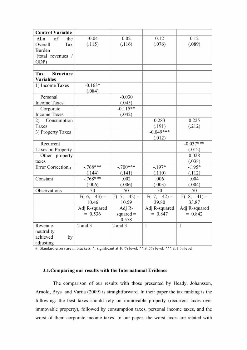
Table 4 verifies the impact of changes in the tax mix over real GDP per capita

growth. In relation to real GDP per capita growth, corporate income taxes look to be the

worst of them, followed by taxes in the capital stock (mainly recurrent ones). The policy

prescription here is clear: changing the tax system toward consumption taxes, or

personal income tax, can improve economic growth.

Table 4: The Effect of Changes in the Tax Mix over Growth.

Dependent variable: growth rate of real GDP per capita

(1) (2) (3) (4)

Baseline Model ΔLn of per worker Physical Capital (kpea)

1.81** (.857)

1.29 (.840)

0.39 (.494)

0.53 (.509)

Δ4Ln of Human Capital (illiteracy rate of population over 15 years old)

0.09 (.084)

0.004 (.091)

-0.02 (.048)

-0.02 (.049)

ΔLn of Economically Active Population (pea)

1.50 (1.34)

1.36 (1.28)

0.55 (.771)

0.75 (.801)

Control Variable ΔLn of the Overall Tax Burden (total revenues / GDP)

-0.04 (.115)

0.02 (.116)

0.12 (.076)

0.12 (.089)


1) Income Taxes -0.163* (.084)


-0.030 (.045)


-0.115** (.042)


0.283 (.191)

0.225 (.212)

3) Property Taxes -0.049*** (.012)

Recurrent Taxes on Property

-0.037*** (.012)

Other property taxes

0.028 (.038)

Error Correction-1 -.768*** (.144)

-.700*** (.141)

-.197* (.110)

-.195* (.112)

Constant -.768*** (.006)

.002 (.006)

.006 (.003)

.004 (.004)

Observations 50 50 50 50 F( 6, 43) =

10.46 F( 7, 42) =

10.59 F( 7, 42) =

39.80 F( 8, 41) =

33.87 Adj R-squared

= 0.536 Adj R-

squared = 0.578




2 and 3 2 and 3 1 1


3.1.Comparing our results with the International Evidence

The comparison of our results with those presented by Heady, Johansson,

Arnold, Brys and Vartia (2009) is straightforward. In their paper the tax ranking is the

following: the best taxes should rely on immovable property (recurrent taxes over

immovable property), followed by consumption taxes, personal income taxes, and the

worst of them corporate income taxes. In our paper, the worst taxes are related with

both capital stock (recurrent taxes) and corporate income taxes. And the best ones are

related to consumption and personal income taxes.

Besides some differences, the policy prescriptions are very similar between our

findings and those of Heady at all (2009). Both papers suggest that a change toward

consumption taxes would improve growth. And both paper strongly advice against taxes

over corporate income.

Acosta-Ormaechea and Yoo (2012) investigate the relation between changes in

tax composition and long-run economic growth (a panel of 69 countries with at least 20

years of observations in the period 1970-2009). They find that increasing income taxes

while reducing consumption and property taxes is associated with slower growth over

the long run. They also conclude that social security contributions and personal income

taxes have a stronger negative impact over growth than corporate income taxes. They

suggest that a shift from income taxes to property taxes has a strong positive association

with growth. Furthermore, a reduction in income taxes while increasing value added

and sales taxes is also associated with faster growth.

Angelopoulos, Economides and Kammas (2007) present an endogenous

growth model to study the growth effects of the composition of government expenditure

and the associated tax burden. They estimate the model using 5 years average data from

a set of 23 OECD countries during the period 1970 to 2000. In relation to the tax

burden, their econometric results suggest that labor income tax rates are negatively

related to growth, whereas capital income and corporate income taxes rates are usually

positively related to growth.

Ojede and Yamarik (2012) estimates a panel data model for states in the United

States, and find that property taxes lowered both short and long run growth, sales taxes

lowered long run growth, and income taxes did not have any effect in short and long run

economic growth.

Xing (2012) estimates the effects of revenue-neutral tax structure changes on

the long-run level of income per capita. The data set refers to yearly panel data

observations for 17 OECD countries over the period 1970-2004. In contrast to previous

studies, he did not find a robust ranking of different types of taxes in terms of their

growth effects. The econometric results did not provide compelling evidence favoring

consumption taxes over income taxes, or favoring personal income taxes over corporate

income taxes. The only robust result appears to be that shifts in tax revenue towards

property taxes are associated with a higher level of income per capita in the long run.

Table C resume the main findings of the literature about tax and growth.

Table C: International Results about Tax and Growth

Tax over: Personal

income

Corporate

income

Consumption Property Capital

income

Angelopoulos,

Economides and

Kammas (2007)

- (labor

income

tax)

+ +

Heady, Johansson,

Arnold, Brys and

Vartia (2009)

- - + +

Acosta-Ormaechea and

Yoo (2012)

- - + +

Ojede and Yamarik

(2012)

No

effect

No effect - (long run) - (short

and long

run)

Xing (2012) No

evidence

No

evidence

No evidence + (long

run)

Our Results + - + -

4. The Channel Between the Tax Burden and Growth

An important question is about the channel from which taxes affect growth. In

this section we estimate the impact of taxes over investment, labor participation and

total factor productivity.

Table 5 presents the effect of taxes over both the labor force participation rate

(the rate between economically active population and the population over 15 years old)

and the rate of private investment to the capital stock11. The labor force participation

data is easy to construct and relies in official data from Brazilian Institute of Geography

and Statistics (IBGE). However, there are a lot of problems associated with the

construction of the private investment data for the Brazilian economy12. The private

investment series adopted here was kindly provided by the Department of

Macroeconomics at Institute for Applied Economic Research13. The private investment

series adopted here excludes from the investment the amounts spent by the government

and by state owned companies. Santos and Pires (2009), and Santos et al. (2011),

provide more information about the construction of the private investment series.

The first line of Table 5 provides us with information about the effect of the

overall tax burden over both the labor rate participation and the rate of private

investment to capital stock. In all four regressions this effect is negative, but statistically

not significant. Column 1 states that increases in the personal income tax decreases

labor force participation rate. Column 2 suggests that increases in both consumption and

recurrent taxes would increase labor force participation rate, but the coefficient of

consumption taxes is much bigger suggesting a higher impact of this variable. In other

words, if we change taxes from personal income to consumption we would expect an

increase in the labor force participation rate, which is clearly a pro-growth tax policy.

Still in Table 5, columns 3 and 4 verify the tax effect over the rate of private investment

to capital stock. None of the relations are statistically significant (in Table 7 we will

explore in more details this relation).

Table 5: The Tax Channel over Economic Variables

Dependent

Variable:

Ln of the Labor

Participation

Rate (1)

Ln of the Labor

Participation

Rate (2)

Ln (Private

Investment / k)

(3)

Ln (Private

Investment / k)

(4)

Ln of the -0.02 -0.006 -0.21 -0.91

11 The use of the rate between private investment to the capital stock of economically active population (kpea) does not change qualitatively the econometric results. 12 I acknowledge here Roberto Ellery Jr., Victor Gomes, Jose Roberto Afonso, and Rodrigo Orair for their kindly help to understand the problems associated with the private investment data and for their help providing me with their time series data. 13 This series was provided by the head of the department, Dr. Claudio Hamilton dos Santos and Researcher Vinícius Augusto Lima de Almeida.

Overall Tax Burden (total revenues / GDP)

(.031) (.047) (.489) (.740)


1) Income Taxes

.345

(.329)


-.027**

(.012)


-.019

(.012)


.170*

(.093)

-1.037 (1.251)

3) Property Taxes


.012*

(.006)

.105 (.067)


.014

(.019)

-.092 (.193)

Constant -.723

(.039)

-.411**

(.172)

117.68*

(60.02)

71.38

(48.08)

Observations 54 54 50 50

F( 5, 48) =

8.97

F( 6, 47) =

7.00

F( 12, 37) =

100.01

F( 14, 35) =

107.81

Adj R-squared

= 0.429

Adj R-squared

= 0.404

Adj R-squared

= 0.960

Adj R-squared

= 0.968


2 and 3 1 2 and 3 1

#: Standard errors are in brackets. *: significant at 10 % level; ** at 5% level; *** at 1 % level. In the labor participation rate equations the regressions included a linear and a quadratic trend. In the private investment equations the regressions included the GDP, the price index, physical and human capital, the size of economically active population, an interest rate (selic rate), and four lags of the private investment.

Table 6 takes a close look about changes in the tax mix over changes in both

the labor force participation rate and in the rate of private investment to physical capital

stock. In the first line all four specifications suggest a negative impact of overall tax rate

over both labor participation and private investment. Column 1 and 2 straights a pro-

growth tax policy: changing the tax mix from personal income to consumption taxes

would increase labor force participation rate. However, Column 4 suggests that an

increase in consumption tax would decrease investment, which is clearly a bad idea in

terms of economic growth. The joint analysis of Tables 5 and 6 suggest that increases in

the recurrent taxes on property would have the double benefit of increase both the labor

force participation rate and the private investment rate.

Maybe our private investment series is not capturing the real investment in the

economic sense of the term. Let’s explore this idea better in Table 7.

Table 6: The Effect of Changes in the Tax Mix over Economic Variables.

Dependent variable: growth rate of the labor force participation

ΔLn of the

Labor

Participation

Rate (1)

ΔLn of the

Labor

Participation

Rate (2)

ΔLn (Private

Investment /

k) (3)

ΔLn (Private

Investment / k)

(4)

ΔLn of the Overall Tax Burden (total revenues / GDP)

-0.05** (.021)

-0.02 (.030)

-0.89** (.337)

-1.50***


1) Income Taxes .246 (.205)


-.020*** (.006)


.005 (.009)


.147** (.059)

-1.384** (.580)

3) Property Taxes Recurrent Taxes on Property

.006* (.004)

.160** (.047)

Other property -.015 -.181

taxes (.015) (.148) Error Correction-1 -.424***

(.114) -.472***

(.119) -.883***

(.225) -.392** (.187)

Constant .0004 (.001)

.0003 (.001)

.022 (.030)

-.047** (.022)

Observations 53 53 49 49 F( 4, 48) =

12.59 F( 5, 47) =

7.74 F( 9, 39) =

5.32 F( 11, 37) =

14.28 Adj R-squared

= 0.471 Adj R-

squared = 0.393




2 and 3 1 2 and 3 1


An important issue is to precisely understand the concept of private investment.

If an individual build a house to live, or spend some money improving it, this is not an

investment in the economic sense. Investment is something that will increase the

production of the economy. However, our private investment series does not take it into

account. To deal with this problem Table 7 disentangle investment in two components:

a) construction; and b) machinery and equipments14. More details about the problems

associated to private investment time series, and how this new investment series was

constructed can be obtained in Santos et al. (2015)15.

Table 7 reproduces the investment equations for both construction and

machinery and equipments. The results are very clear in pointing out different behavior

for these investment series. In all for specifications the overall tax burden negatively

affects investment. Columns 1 and 2 suggest that changing taxes to consumption would

improve investment in construction. However, columns 3 and 4 suggest that the

investment in machinery and equipments are negative affected by the overall tax rate,

but not for the tax mix. It is important to observe that if we change the tax mix to

consumption the overall tax rate lost its statistical significance to decrease investment.

In other words, a change of the tax mix toward consumption taxes would increase

investment. 14 This new dataset was kindly provided by Dr. Claudio Hamilton dos Santos and Vinícius Augusto Lima de Almeida. 15 They argue that investments made in construction are majorly made by families and government, and that the investments in machinery and equipments are mainly due to non-financial companies.

Table 7: The Tax Channel over Investment

Dependent

Variable:

Ln of

Construction

(1)

Ln of

construction

(2)

Ln machinery

and

equipments (3)

Ln machinery

and

equipments (4)


-0.42*

(.223)

-0.03

(.252)

-0.68*

(.345)

-0.07 (.411)


1) Income Taxes


-.057

(.087)

-.136

(.134)


.016

(.085)

.137

(.131)


1.002*

(.562)

1.04 (.915)

3) Property Taxes

.859

(.987)

.772 (1.60)

Recurrent Taxes on Immovable Property


Constant 3.86***

(.273)

4.71***

(.417)

3.65***

(.422)

4.63***

(.679)

Observations 54 54 54 54

F( 5, 48) =

40.87

F( 5, 48) =

44.18

F( 5, 48) =

57.02

F( 5, 48) =

54.42

Adj R-squared

= 0.790

Adj R-squared

= 0.840

Adj R-squared

= 0.834


2 and 3 1 2 and 3 1

#: Standard errors are in brackets. *: significant at 10 % level; ** at 5% level; *** at 1 % level. All the regressions included a linear and a quadratic trend.

In Table 8 we verify the impact of changes in the tax mix over investment in

construction and machinery and equipments. Again a change to consumption taxes

would improve investment growth.


Dependent variable: growth rate of the labor force participation

ΔLn of the

construction

(1)

ΔLn of the

construction

(2)

ΔLn

machinery and

equipments

(3)

ΔLn

machinery and

equipments (4)


-0.22* (.120)

-0.07 (.124)

-0.43 (.205)

-.005 (.222)


1) Income Taxes Personal Income Taxes

-.053 (.038)

-.112* (.065)


-.055 (.049)

-.003 (.084)


.572** (.282)

1.223* (.599)

3) Property Taxes .010 (.017)

.043 (.030)



Error Correction-1 -.182* (.095)

-.150 (.094)

-.271** (.105)

-.251** (.104)

Constant .004 (.005)

.004 (.005)

.007 (.009)

.005 (.009)

Observations 53 53 53 53 F( 4, 48) =

6.94 F( 4, 48) =

8.57 F( 4, 48) =

6.60 F( 4, 48) =

6.67


Adj R-squared =

0.367

dj R-squared = 0.301



2 and 3 1 2 and 3 1


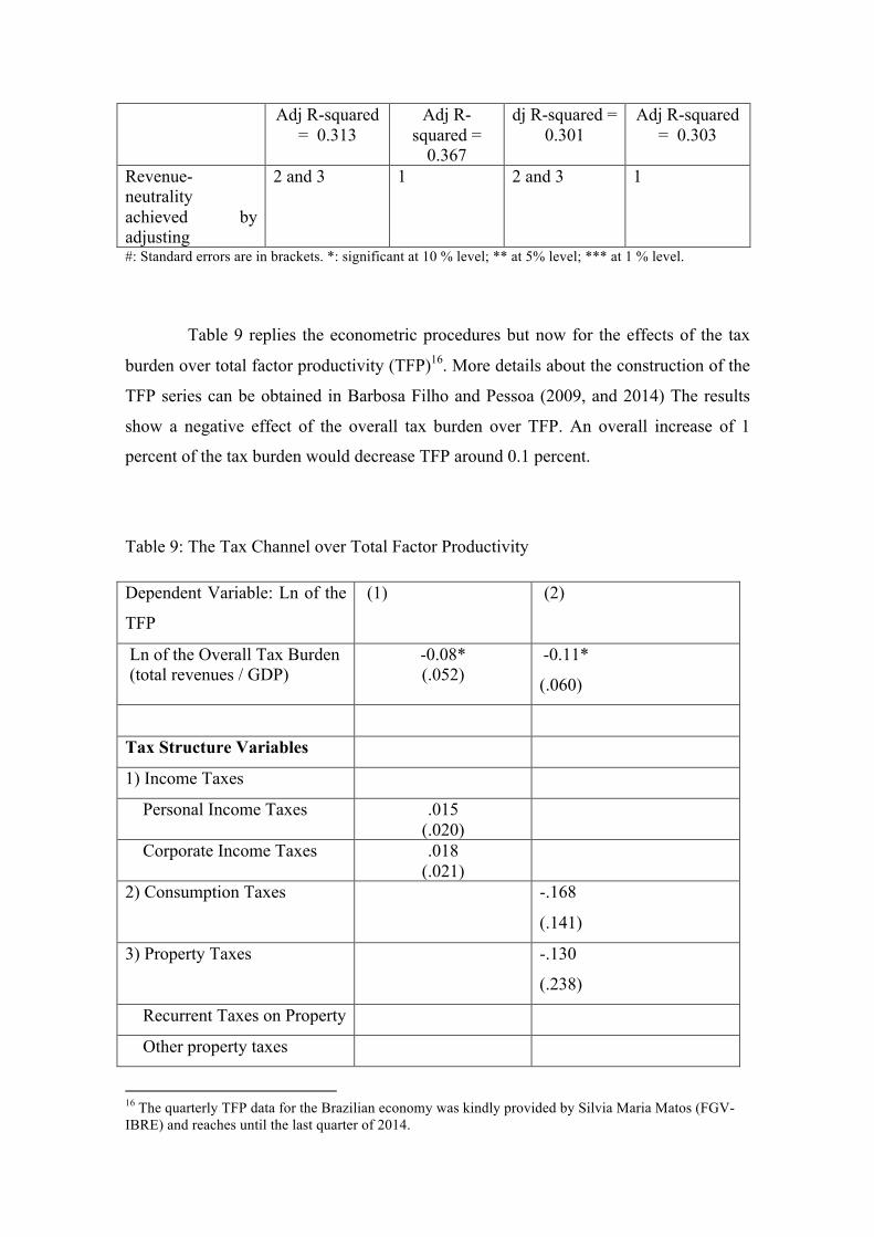
Table 9 replies the econometric procedures but now for the effects of the tax

burden over total factor productivity (TFP)16. More details about the construction of the

TFP series can be obtained in Barbosa Filho and Pessoa (2009, and 2014) The results

show a negative effect of the overall tax burden over TFP. An overall increase of 1

percent of the tax burden would decrease TFP around 0.1 percent.

Table 9: The Tax Channel over Total Factor Productivity

Dependent Variable: Ln of the

TFP

(1) (2)


-0.08* (.052)

-0.11*

(.060)


1) Income Taxes

Personal Income Taxes .015 (.020)

Corporate Income Taxes .018 (.021)

2) Consumption Taxes -.168

(.141)

3) Property Taxes -.130

(.238)



16 The quarterly TFP data for the Brazilian economy was kindly provided by Silvia Maria Matos (FGV-IBRE) and reaches until the last quarter of 2014.

Constant .950**

(.370)

.717*

(.374)

Observations 51 51

F( 6, 44) = 290.78 F( 6, 44) = 296.74

Adj R-squared =

0.972



2 and 3 1

#: Standard errors are in brackets. *: significant at 10 % level; ** at 5% level; *** at 1 % level. All the regressions included a linear and a quadratic trend and a lag for the TFP.

Table 10 takes a close look about changes in the tax mix over changes in the

TFP. The overall tax burden affects negatively the TFP. But the tax mix sounds not to

be important in relation to their negative effect over TFP.


Dependent variable: growth rate of the Total Factor Productivity

(1) (2)


-0.064 (.046)

-.08* (.051)

Tax Structure Variables 1) Income Taxes Personal Income Taxes .008

(.014)

Corporate Income Taxes .002 (.020)

2) Consumption Taxes -.112 (.117)

3) Property Taxes -.005 (.006)

Recurrent Taxes on Property Other property taxes Error Correction-1 -.359***

(.157) -.337** (.158)

Constant .004* (.002)

.004 (.002)

Observations 50 50

F( 4, 45) = 2.29 F( 4, 45) = 2.31 Adj R-squared = 0.095 Adj R-squared =

0.096 Revenue-neutrality achieved by adjusting

2 and 3 1


5. Conclusion

This paper analyses the effect of the tax burden over GDP per capita and its

growth. Our paper follows the recent development in the literature of taxes and growth

as stated by Heady, Johansson, Arnold, Brys and Vartia (2009).

The econometric results pointed out for a negative effect of overall tax burden

over both the level and the growth of GDP per capita. In relation to the level of GDP per

capita, this negative effect ranges around -0.3. In other words, an increase of 1% in the

overall tax burden decreases real GDP per capita by 0.3%. This is a strong and

statistically significant negative effect of overall tax burden over GDP per capita. In

relation to the growth level of GDP per capita, the change in the overall tax burden has a

negative impact close to 0.15.

Furthermore, additional econometric results pointed out that a revenue neutral

fiscal policy which changes the tax structure toward consumption taxes and personal

income taxes would improve economic growth. Besides that, we strongly recommend

against both taxes over the capital stock (mainly the recurrent ones) and the corporate

income taxes.

Finally, we were able to demonstrate that both the overall tax burden and its tax

mix have negative impact over the labor force participation rate and private investment.

And the overall tax burden has negative and statistically significant effects over total

factor productivity. Decrease the overall tax burden, and change the tax mix toward

consumption and personal income taxes, has the potential to improve real GDP and its

growth rate for the Brazilian economy.

Bibliography

Acosta-Ormaechea, S. and Yoo, J. (2012) “Tax Composition and Growth: A Broad

Cross-Country Perspective”. IMF Working Paper, WP/12/257, Fiscal Affairs

Department, October.

Amaral, G.L., Olenike, J.E., Amaral, L.M.F. (2013) “Quantidade de Normas Editadas

no Brasil: 25 anos da Constituição Federal de 1988”. Instituto Brasileiro de

Planejamento Tributario, Outubro.

Angelopoulos, K. and Economides, G., and Kammas, P. (2007) "Tax-spending policies

and economic growth: Theoretical predictions and evidence from the OECD". European

Journal of Political Economy, vol. 23(4), pages 885-902, December.

Barbosa Filho, F.H., and Pessôa, S.A. (2009) “Série de Horas Mensais da Economia

Brasileira”. Dezembro. FGV-IBRE Nota Tecnica, no.1.

Barbosa Filho, F.H., and Pessôa, S.A. (2014) “Pessoal Ocupado e Jornada de Trabalho:

uma releitura da evolução da Produtividade no Brasil”. Revista Brasileira de Economia,

v. 68, n. 2.

Heady, C., Arnold, J., Brys, B., Johansson, A., Schwellnus, C., and Vartia, L. (2011)

“Tax Policy for Economic Recovery and Growth”. Economic Journal, v. 121, issue 550,

pages: F59-F80.

Heady, C., Johansson, A., Arnold, J., Brys, B., and Vartia, L. (2009) “Tax Policy for

Economic Recovery and Growth”. University of Kent School of Economics Discussion

Papers, December, KDPE 0925.

Kaplow, L. (2010) “The theory of taxation and public economics”. Princeton University

Press, 472 p.

Messias, L. (2013) “Contencioso Tributario no Brasil é muito superior ao dos EUA”.

Consultor Juridico, Novembro, (http://www.conjur.com.br/2013-nov-21/lorreine-

messias-contencioso-tributario-brasileiro-superior-eua).

Morandi, L.; Reis, E. J. (2004) “Estoque de capital fixo no Brasil - 1950-2002”. XXXII

Encontro Nacional de Economia - ANPEC, 07-10 de dezembro, João Pessoa.

World Bank. “Doing Business (2015)”. 12ª edition. Online:

http://portugues.doingbusiness.org/~/media/GIAWB/Doing%20Business/Documents/A

nnual-Reports/English/DB15-Full-Report.pdf.

Ojede, A. and Yamarik, S. (2012) "Tax policy and state economic growth: The long-run

and short-run of it". Economics Letters, vol. 116(2), pages 161-165.

Orair, R. O., Gobetti, S.W., Leal, E.M. e Silva, W.J. (2013) “Carga Tributária

Brasileira: Estimação e Análise dos Determinantes da Evolução Recente - 2002 –

2012”. Texto para Discussao do IPEA, TD 1875, Rio de Janeiro, October.

Santos, C.H.; Modenesi, A.M.; Squeff, G.; Vasconcelos, L.; Mora, M.; Fernandes, T.;

Moraes, T.; Summa, R.; and Braga, J. (2015) “Revisitando a dinâmica trimestral do

Investimento no Brasil: 1996-2012”. Texto para Discussao do Instituto de Economia da

UFRJ, no. 5, Abril. Forthcoming in Revista de Economia Politica.

Santos, C. H.; Orair, R. O.; Gobetti, S. W.; Ferreira, A. S.; Rocha, W. S.; and Britto, J.

M. (2011) “Uma metodologia de estimação da formação bruta de capital fixo das

administrações públicas brasileiras em níveis mensais para o período 2002-2010”. Texto

para Discussao do IPEA, no. 1660.

Santos, C. H.; and Pires, M. C. (2009) “Qual a sensibilidade dos investimentos privados

a aumentos na carga tributária brasileira? Uma investigação econométrica”. Revista de

Economia Política, vol. 29, nº 3 (115), pp. 213-231, julho-setembro.

Xing, J. (2012) "Tax structure and growth: How robust is the empirical evidence?"

Economics Letters, vol. 117(1), pages 379-382.

Annex A: Relation of taxes and respectives classifications

Esfera Incidencia IncTipo Simples Impostos sobre o

Consumo TOTAL

GF Impostos sobre os produtos

IPI


II


IE


Cofins


Cide


CS -‐ Outras


CE -‐ Outras

GF Outros impostos sobre a produção

SalEdu


Demais folha


Sistema S


Taxas -‐ Polícia


Taxas -‐ Serviços


CS -‐ Outras


CE -‐ Outras

GE Impostos sobre os produtos

ICMS

GE Impostos sobre os produtos

ISS

GE Outros impostos sobre a produção

Outros impostos e taxas sobre a produção

GM Impostos sobre os produtos

ISS

GM Outros impostos sobre a produção

Taxas

Impostos sobre a

Renda TOTAL

GF Impostos sobre a renda

IRPF


IRPJ


IRRF


CE -‐ Outras

GF Outros impostos correntes sobre a renda e propriedade

CSLL

GE Impostos sobre a renda (governos estaduais retem mas nao repassam ao Federal)

IRRF

GM Impostos sobre a renda (governos municipais retem mas nao repassam ao Federal)

IRRF

IR sobre rendimentos do trabalho

IR sobre rendimentos do capital]

Imposto Recorrente

sobre a Riqueza (Imposto sobre Propriedade)

TOTAL


ITR


DPVAT

GE Outros impostos correntes sobre a renda e propriedade

IPVA

GE Outros impostos correntes sobre a renda e propriedade

IPTU

GM Outros impostos correntes sobre a renda e propriedade

IPTU

Imposto Sobre

Movimentacao Financeira

TOTAL


CPMF


IOF

Imposto Nao

Recorrente sobre a Riqueza (Imposto Sobre o Capital)

TOTAL

GF Impostos de capital IC GE Impostos de capital ITCD GE Impostos de capital ITBI GM Impostos de capital ITBI GM Impostos de capital Contribuição de

melhoria

********* Ikperc = imp.capital perc + imp.propriedade perc

Contribuicao Social e

Previdencia TOTAL

GF Contribuições sociais FGTS GF Contribuições sociais PIS/Pasep GF Contribuições sociais CS -‐ RGPS GF Contribuições sociais CS -‐ RGPS GF Contribuições sociais CS -‐ RGPS GF Contribuições sociais CS -‐ RPPS GF Contribuições sociais CS -‐ RPPS GF Não Classificado Dívida ativa -‐ outros GE Contribuições sociais Cont. Previdenciárias GE Outros impostos

sobre a produção Outras contribuições

sociais GM Contribuições sociais Contribuições

Previdenciárias GM Outros impostos

sobre a produção Outras contribuições

sociais GM Outros impostos

sobre a produção Contribuições

econômicas

********* Iconprodperc = imp.consumo perc + contrib social e previdencia perc