Tasks

International Trade, Technology, and

Distribution

Code EBC 4036, period 2

Academic Year: 2016/2017

BEFORE THE FIRST MEETING, READ the course book and Task 1 AND STUDY THE

LITERATURE MENTIONED THERE: BHAGWATI ET AL. CHS.2, 3. Prepare questions

for the first meeting on the procedures, the tasks and the literature.

© Thomas Ziesemer 2016 All rights reserved. No part of this publication may be reproduced, stored in a retrieval system, or transmitted, in any form or by any means, electronic, mechanical photocopying, recording or otherwise, without the prior written permission of the publishers.

1

International Trade, Technology, and Distribution (EBC4036)

Table of contents:

Tasks.

Number Title Meeting Page

1 Comparative advantage: Ricardo is the basis 1, 2

2 Justification of policy interference, adequate instruments … 2, 3 2

3 Heckscher-Ohlin and wage inequality, 4 10

3b TAKING STOCK: What have we done so far and where are we going to? 5 16

4 Trade, factor movements, technical change, specific factors, oil … 5 14

5 Heckscher-Ohlin, technical change and factor movements in history 6 15

6 Non-traded goods, globalization of trade and offshoring of tasks 7 22

7 Case study: ETS, CDM, and eucalyptus. What’s going wrong? 8 25

Empirical tasks I:

Presentations by each student 5 minutes before the break 9

8 North-South tech. transfer, product cycle, & the world distribution … 9, 10 39

9 Learning by doing, technological leadership, and leapfrogging 11, 47

10 Imperfect competition, intra-industry trade, and R&D 12a 50

11 Gains from trade under uncertainty, protectionism pushing food prices 12b 51

Presentations of empirical tasks II 13

2

Tasks

Task 1 Comparative advantage

We will tackle several interesting problems during the course: Trade and environment;

uncertainty in food supply and prices; non-traded goods and globalization; learning-by-doing,

leadership and leapfrogging. To understand the articles related to these problems, it is

necessary to understand the Ricardian trade model of comparative advantage:

Literature: Bhagwati et al. (1998), chaps. 2-3.

Empirical Task: Calculate Balassa’s revealed comparative advantage index and compare it to

that of Vollrath in Wörz (2005) (see eleum) for the country of your case study.1

Task 2

Justification of policy interference, adequate instruments, and applications to trade

related environmental problems

Literature:

- Södersten and Reed 1994, p. 30-32.

- Hierarchy of Policies: Bhagwati et al. (1998), chap. 17. Appendix on Bhagwati et al., below.

- Appendix below: Environmental externalities, taxes and subsidies in the autarkic Ricardian

economy.

- Pugel, T., Chapter on Trade and the Environment.

- Production Externalities, Monopoly: Bhagwati et al. (1998), chaps. 22, 23. Appendix below

on Bhagwati et al. (1998) regarding chap. 22, 23.

Appendix:

Environmental externalities, taxes and subsidies in the autarkic Ricardian economy

The modified Ricardian model: Disutility from emissions caused by production of good 1

(lower index indicates a sector in production and a derivative in utility)

(1) U(C1, C2)+ V(E),U1,2 >0,V’< 0

(2) C1 = F1(L1),

(3) C2 = F2(L2)

(4) E = P(C1),

(5) L1 + L2 – L = 0

The figure collects the results following below.

1 Wörz, Julia; Dynamics of Trade Specialization in Developed and Less Developed Countries. Emerging Markets

Finance and Trade, May-June 2005, v. 41, iss. 3, pp. 92-111.

3

We proceed in two steps: 1. What would a benevolent and omniscient central planner do. 2.

How does market equilibrium come to the same result?

Central Planner’s OPTIMUM

Lagrange function Γ for welfare maximization is (Fi is production function of good i, Li is

labour input in sector i; Fi’ is marginal product of labour, P is pollution, P’is marginal

pollution from good 1, U utility, V (dis-) utility from emissions; Ui marginal utility of good i,

λ is the Lagrange multiplier, ∂ indicates a partial derivative):

Γ = U[F1(L1), F2(L2)] + V[P(F1(L1)] + λ(L-L1-L2)

Take paper and pen(cil) and calculate and interpret the following results.

1/ L =

U1F1' + V'P'F1'(L1) - λ = 0 (6)

2/ L = U2F2' - λ = 0 (7)

Eliminating the Lagrange multiplier yields:

U1(.)F1' + V'P'F1'(L1) - U2(.)F2' = 0 (8)

a1 a1 a2 where ai are productivities.

U1[F1(L1), F2(L2)]a1 + V'(E)P'(C1)a1 = U2[F1(L1), F2(L2)]a2

The marginal utility of L1 is diminished by V'P'.

U1F1' + V'P'F1' = U2F2' (8') Division by U2 and F1’ yields

U1/U2 + (V'P')/U2 = F2'/F1’ (8'')

- U1/U2 = -a2/a1 + (𝑽′𝑷′)/𝑼𝟐⏟ −

, (8''')

4

As the last term is negative, this is more negative than without V(E). From (2), (3) and (5):

L1 + L2 – L= C1/a1 + C2/a2 –L = 0

gives PPF: C1 = La1- C2 a1/a2

L1opt

, L2opt

is where the indifference curve without the V’-part intersects with the PPF in the

figure, at lower C1 and larger C2 than without taxes on C1.

How do we get the optimal solution?

POLICY SOLUTION 1: TAXING PRODUCTION OF THE POLLUTING GOOD

Household: U(C1, C2) + V(E)

(9) P1C1 + P2C2 - wL - ∑πi – T =0

(10) U1 = λP1 (11) U2 = λP2

U1/U2 = P1/P2 (12)

Firm 1:

π1 = (P1 - t) F1(L1) - wL1 (13)

π1/L1 = (P1 - t) F1' - w = 0 (14)

Firm 2:

π2 = P2 F2(L2) - wL2 (15)

π2/L2 = P2 F2' - w = 0 (16)

Eliminate wages from (14) and (16):

(P1 - t)F1' = P2F2' (17)

(P1 - t)/P2 = F2'/F1' (17')

P1/P2 = F2'/F1' + t/P2 (17'')

Government: tF1(L1) = T (18) Less pollution, less government revenue.

(12) and (17’’) yield P1/P2 = U1/U2 = F2'/F1' + t/P2 , (19)

How high is the optimal tax rate? (19) equals the optimal rule (8''') for the t/P2 = -(V'P')/U2 and

figure 1 depicts the equilibrium which is an optimal solution because of the optimal tax.

(Pigou)

5

POLICY SOLUTION 2:

SUBSIDIZING PRODUCTION REDUCTION OF THE POLLUTING GOOD

Household: U(C1, C2) + V(E)

P1C1 + P2C2 - wL - ∑πi - T = 0

U1 = λP1 U2 = λP2

U1/U2 = P1/P2

Firm 1:

π1 = P1F1(L1) + s[C1* - F1(L1)] - wL1 (20)

C1* is the market equilibrium value if there is no policy.

π1/L1 = P1F1' - sF1' - w = 0, (21)

Firm 2: as above in (16):

P2F2' = w (22)

Equalising wages in (21) and (22) yields:

(P1 - s)F1' = P2F2' (23)

Dividing by F1' and P2 yields:

P1/P2 - s/P2 = F2'/F1' (23')

P1/P2 = F2'/F1' + s/P2 (23'')

U1/U2 = F2'/F1' + s/P2 (24)

s > 0 is efficient if it equals t in solution 1 - see (19) - and s/P2 equals -(V'P')/U2 from (8'''). In

that case, figure 1 applies again.

Do the basic computations yourself to get the following solutions.

POLICY SOLUTION 3: SUBSIDY FOR CONSUMPTION OF THE CLEAN GOOD C2

Before household conditions were never affected, but now the household pays (P2 - s)C2:

U1/U2 = P1/(P2 - s) or U2/U1 = (P2 - s)/P1 (25)

Firms: From first–order conditions and elimination of wages:

P1F1' = P2F2' ; P1/P2 = F2'/F1' (this is also the slope of the PPF)

6

Insertion of the last equation into (25) yields

U2/U1 = F1'/F2' - s/P1

With constant F2'/F1' the "good value" of s enhances U1/U2 (or reduces U2/U1) to the optimal

level. For P1 = 1 the producer price P2 must be higher now than in all previous cases; the

consumer price is the same. Fig. 1 applies only after subtracting s from the price of good 2.

POLICY SOLUTION 4: SUBSIDY FOR PRODUCTION OF THE CLEAN GOOD C2

Households:

U1/U2 = P1/P2 , as above

Firm 1: P1F1' - w = 0 (26)

Firm 2: (s + P2)F2'-w = 0 (27)

From (26) and (27):

P1F1' = (P2 + s)F2' or

F1'/F2' = (P2 +s)/P1

F1'/F2' = U2/U1 + s/P1

or U2/U1 = F1'/F2' - s/P1

Here the optimal level of s is equivalent to the subsidy for consumption of good C2.

7

Appendix on Bhagwati et al. (1998)

Ch.17

The most important consideration here is that world prices may differ from consumer prices

and both may differ from producer prices. In each case, we have to think clearly about which

price is relevant for producers, consumers and the world. The economy deals with the world

market in terms of world market prices. All taxes, subsidies and tariffs are transactions

between domestic individuals.

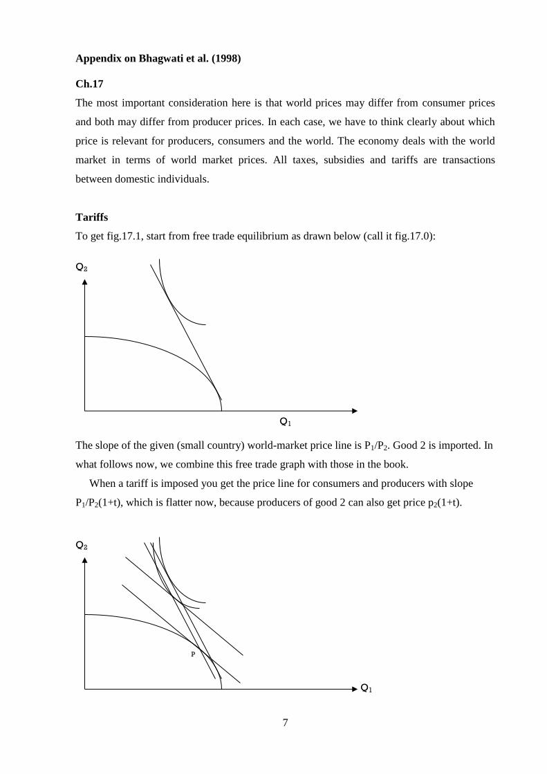
Tariffs

To get fig.17.1, start from free trade equilibrium as drawn below (call it fig.17.0):

Q2

Q1

The slope of the given (small country) world-market price line is P1/P2. Good 2 is imported. In

what follows now, we combine this free trade graph with those in the book.

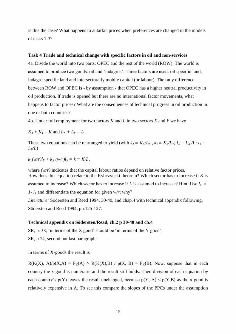
When a tariff is imposed you get the price line for consumers and producers with slope

P1/P2(1+t), which is flatter now, because producers of good 2 can also get price p2(1+t).

Q2

P

Q1

8

The production point P has moved northwest. From there take the world price line along

which you can trade to come to a point at which the slope of the indifference curve and the

tariff-inclusive line are tangential. Paying tax revenues to households as lump-sum transfer at

value T the government budget is tp2q2-T = 0. The consumption point is in the south-east to

that of free trade. Welfare is lower although we have tariff revenues now! You get your money

back but the effect of the distorting change of the producer price remains and it shifts the

budget line of households down and to the left.

Production tax cum subsidy

Start out again from the free trade equilibrium with world price ratio P1/P2. The government

by assumption gets tax revenues tp1q1 from firms producing good 1 and rebates them to

households in the form of the subsidy: sp2q2. For an arbitrarily chosen value t, we obtain the

value of s in principle from the government’s budget condition: tp1q1 = sp2q2. Taxing

production of good 1 and subsidization of good 2 yields producer prices: (1-t)P1/[P2(1+s)].

For producers the price line becomes flatter. Production moves to the northwest. From the new

production point, draw the world price line again. Then find an indifference curve, which is

tangent to it, because consumer prices are not affected by the tax-subsidy combination, which

is for production only. Consumption moves southwest when compared to autarky. Welfare is

lower again; for households there is only an income effect.

Q2

Q1

Consumption tax cum subsidy

Start out again from the free trade equilibrium with price ratio P1/P2. Tax consumption of

good 2 and subsidize good 1: (1-s)P1/[P2(1+t)]. For producers the price line is unchanged.

Consumers have a flatter price line. We have to find a point on the world price line where the

flatter consumer price line is tangential. Welfare is lower again.

9

Q2

Q1

Factor tax cum subsidy for one sector

Suppose countries work with two factors, K and L, and production functions of the sectors are

F(K1, L1) and G(K2, L2). Under free factor mobility between the sectors both sectors will have

the same marginal value product (lower indices of F and G indicate partial derivatives) equal

to factor prices R and W: for capital, p1FK = R = p2GK , and for labour, p1FL= W = p2GL. The

slope of the production possibility curve indicates how much of one good is lost if one unit of

K or L is shifted to the other one: -GK / FK = -GL / FL = - p1/p2 ≡ - p.

With given world prices p = p1/p2 and uniform taxes on factor prices in sector 2 it has to

pay for each unit of capital (1+t)R = p2GK, and for labour (1+t)W = p2GL. For the other sector

we have R = p1FK, W = p1FL. By implication we get p = [GK /(1+t)] / FK = [GL /(1+t)]/ FL.

As p is given, the ratios GK / FK and GL / FL must now be higher and the factor allocation has

moved away from the first best of the Figures above. Therefore, we must be under the

production possibility curve as drawn in figure 17.4. IF THIS IS DIFFICULT, DO NOT

WORRY; IT COMES AGAIN IN SIMILAR FORM IN CH.22.

NOTE THAT ALL TAXES IN CH.17 ETC ARE INTRODUCED WITHOUT ANY

REASON TO CORRECT THE MARKET EQUILIBRIUM. THEREFORE, THEY LEAD TO

LOWER WELFARE. THIS IS CHANGED IN CH.22.

Bhagwati et al. ch.22

YOU MAY IGNORE THE FIRST PARA OF CH.22. DP is ‘domestic price ratio’ (285); DRS

is domestic rate of substitution in consumption (the slope of the indifference curve); DRT is

‘domestic rate of transformation in production (the slope of the production possibility

frontier); FRT is the (Free) Trade Rate of Transformation (the slope of the budget line as

defined by the relative prices).

How to get (22.6), the social marginal rate of factor substitution or the slope of the

10

production possibility curve, when taking into account the externalities? The PPC is defined as

Max Q1 = F(K1,L1, Q2), s.t. Q2 = G(K2,L2), K = K1+K2, L=L1+L2. Inserting the constraints into

the objective function – first the production function for good 2, then K2 and L2 from the

resource constraints - yields

Max Q1= F(K1,L1, G(K-K1,L-L1))+λ [Q2- G(K-K1,L-L1)]

through choice of K1 and L1. Taking first-order conditions with respect to K1, L1.

K1: FK + FQGK(-1) – λGK(-1) = 0

L1: FL + FQGL(-1) – λGL(-1) = 0

Solving both equations for –λ and putting them equal yields:

(FK + FQGK(-1))/ GK = (FL + FQGL(-1))/ GL

Actually, this is the same as the first equation in (22.8). Multiplying both sides with GL and

dividing both sides by (FK + FQGK(-1)) yields (22.6). Without the externality FQ you get (22.5)

again.

After equation (22.6) the formulation ‘It is easily seen …’ may be a slight exaggeration.

What you should see is the following: (22.6) consists of two fractions. Do or imagine the

cross-multiplication. Then you get on the left-hand side and on the right-hand side a term -

FQGLGK . If you cancel this term, you can divide by GK again and get the same result as in

equation (22.5). Similarly, you get (22.8) from (22.6) by division of both sides of (22.6) by GL

and by multiplication with the second term in parentheses.

Note that the difference between p.302 and 303 is that in eq. (22.7) the price PP is given.

According to figure 22.1, the optimum has a higher good 1 production than the market

equilibrium (∂F/∂Q2 < 0, negative externality of good 2, because 1/Pp > 1/DRT in the Figure),

but the text has a higher good 2 production in the optimum (∂F/∂Q1 > 0, positive externality of

good 2, because Pp > DRT in the text).

Note that in the middle of page 304 and after equation (22.10) the assumption is that K2

produces a positive externality.

11

Task 3 Heckscher-Ohlin theory, factor price equalization and wage inequality

In the debate on what determines the trade pattern, endowment theory has often been criticized

for doing a bad job. However, which endowments are there and which are the relevant ones? It

is about North-South trade anyway, as you can see from the trade data. For trade and

development, the same things seem to matter.

An electronic engineer applies for a job at an E-company. His first job will be to build

electronic infrastructure in India. Asking for the salary he gets the answer ‘Of course, you will

get as much as your Indian colleague’.

In the debate on wage inequality in the 1990s, one group of economists argues that the

inequality is due to trade liberalization. They use a Heckscher-Ohlin model for their argument.

Consider the two-goods, two-factor model and replace physical by human capital. For which

country does trade liberalization increase the wage inequality measured by the factor-price

ratio of human capital and labour (more and less skilled labour)? Where does the distribution

get more (un-)equal?

Literature: Södersten and Reed 1994, chap.3. Technical appendix below on Södersten/Read.

Empirical task: What are the endowments of your country comparable to those in the adjacent

figures? Take a time series as long as possible. Try to produce such a figure from the data of

your country.

Technical appendix on Södersten/Read, ch.3

p.49: 5th

line from below; my version of the book says ‘higher’, but it should be ‘lower’ or Y

and X should be exchanged. In other prints of the 1994 edition, this is correct. Check yours by

comparison with figure 3.6.

p.50: is the slope at point S in Figure 3.6. At ’ there is more labour and less capital relative

to .

On Figure 3.7: Factor intensity reversal when two sectors only

differ in the CES parameter of the function 1

(1 )Y K AL

From cost minimization in case of A=1 we get (check)

w/r=((1-α)/α)((K/L))1-ρ

with α=.3 and ρ=-1 or -1/2 for the two sector respectively

yields an elasticity of substitution of σ=1/(1-ρ)= 1/2 or 2/3:

12

w/r =((.7)/(.3))(K/L)², w/r =((.7)/(.3))(K/L)1.5

- You may skip figure 3.10 and the text explaining it.

0.0 0.2 0.4 0.6 0.8 1.0 1.2 1.4 1.6 1.8 2.00

1

2

3

4

5

6

7

8

9

k

w/r

13

Development of Thailand's Export Profile, 1960-1989

Export Composition against HR/NR, 1960

Thailand y = 0.7682x + 0.0899

(7.98) (0.23)

R2 = 0.4252-8.00

-6.00

-4.00

-2.00

0.00

2.00

4.00

-8.00 -6.00 -4.00 -2.00 0.00 2.00 4.00

ln(years of schooling/sqkm land)

ln(m

an

ufa

ctu

red

exp

ort

s/p

rim

ary

exp

ort

s)

Export Composition against HR/NR, 1975

Thailand

y = 0.8416x + 1.1452

(10.72) (4.21)

R2 = 0.5721-8.00

-6.00

-4.00

-2.00

0.00

2.00

4.00

-8.00 -6.00 -4.00 -2.00 0.00 2.00 4.00

ln(years of schooling/sqkm land)

ln(m

an

ufa

ctu

red

exp

ort

s/p

rim

ary

exp

ort

s)

Export Composition against HR/NR, 1989

Thailand

y = 0.8522x + 1.3897

(11.82) (6.62)

R2 = 0.6189-8.00

-6.00

-4.00

-2.00

0.00

2.00

4.00

6.00

-8.00 -6.00 -4.00 -2.00 0.00 2.00 4.00ln(years of schooling/sqkm land)

ln(m

an

ufa

ctu

red

exp

ort

s/p

rim

ary

exp

ort

s)

Note: HR = Human resources. NR = Natural Resources. Manufactured exports = UNCTAD SITC categories 5-8, less 68. Years of

schooling per km2 land = average number of years of schooling of the adult population (over 25)/total (not arable) land area of each

country divided by adult population. Sample of 114 countries with pop. > 1 million. T-statistics in parenthesis. Source: Johanna Witte, The

Concept of competitiveness with applications to Thailand (2000), IES MA Thesis, UM. Data from Wood and Berge (1997).

Data are availalble from the UM website, data sources A-Z, WorldDataBank, World Development Indicators.

14

Task 3b TAKING STOCK: What have we done so far and where are we going?

Building blocks:

Comp. adv. models: Ricardian trade model, Heckscher-Ohlin model, Specific factors model;

Taxes, subsidies and tariffs as distortions and correction of distortions: monopoly and

externality

Applications:

Distribution effects of free trade: North-South factor price equalization? (Task 3)

Distribution differences from technical differences: specific versus mobile factors (Task 4)

Distribution effects of technical change: wage inequality (Task 4 and 5)

Distribution effects of free factor movements (Task 5)

Explaining globalization of trade; effects of technology transfer; routinization and outsourcing

threatening the middle class (Task 6)

Emission trading and comparative advantage: from Ricardo to Heckscher-Ohlin. Task 7

More building blocks: Dynamics, imperfect competition, and uncertainty

Changing determinants of trade advantage: imitation gap and product-cycle theory (Task 4)

New products (Task 8)

Learning–by-doing (Task 9)

Scale economies and imperfect competition (Task 10)

Uncertainty (task11)

Applications

Innovation, technology transfer through imitation and population growth moving capital,

affect terms of trade and North-South wages (Task 8)

Distribution effects of demand differences, history of leadership and leapfrogging (task 9)

Intra versus inter-industry trade (Task 10)

Food crisis: Trade policy and speculation in the short and Ricardian growth the long run (task

11)

Objective versus subjective prices.

Karl Marx argued that prices were determined just based on costs (objective prices) and

independently of preferences or demand (not subjective prices). In which of the trade models

15

is this the case? What happens to autarkic prices when preferences are changed in the models

of tasks 1-3?

Task 4 Trade and technical change with specific factors in oil and non-services

4a. Divide the world into two parts: OPEC and the rest of the world (ROW). The world is

assumed to produce two goods: oil and ‘indagros’. Three factors are used: oil specific land,

indagro specific land and intersectorally mobile capital (or labour). The only difference

between ROW and OPEC is - by assumption - that OPEC has a higher neutral productivity in

oil production. If trade is opened but there are no international factor movements, what

happens to factor prices? What are the consequences of technical progress in oil production in

one or both countries?

4b. Under full employment for two factors K and L in two sectors X and Y we have

KX + KY = K and LX + LY = L

These two equations can be rearranged to yield (with kX ≡ KX/LX , kY ≡ KY/LY; lX = LX /L; lY =

LY/L)

kY(w/r)lY + kX (w/r)lX = k ≡ K/L,

where (w/r) indicates that the capital labour ratios depend on relative factor prices.

How does this equation relate to the Rybczynski theorem? Which sector has to increase if K is

assumed to increase? Which sector has to increase if L is assumed to increase? Hint: Use lX =

1- lY and differentiate the equation for given w/r; why?

Literature: Södersten and Reed 1994, 30-40, and chap.4 with technical appendix following.

Södersten and Reed 1994, pp.125-127.

Technical appendix on Södersten/Read, ch.2 p 30-40 and ch.4

SR, p. 38, ‘in terms of the X good’ should be ‘in terms of the Y good’.

SR, p.74, second but last paragraph:

In terms of X-goods the result is

R(K(X), A)/p(X,A) = FK(A) > R(K(X),B) / p(X, B) = FK(B). Now, suppose that in each

country the x-good is numéraire and the result still holds. Then division of each equation by

each country’s p(Y) leaves the result unchanged, because p(Y, A) < p(Y,B) as the x-good is

relatively expensive in A. To see this compare the slopes of the PPCs under the assumption

16

that A produces more X than B; then the PPC of A must be steeper, and therefore p(X)/p(Y)

too. Thus, the result holds even more in terms of Y-goods.

SR, p.75, result (iii)

This result follows from the profit maximization of the x and the y sector: both equate the

marginal value product to the nominal wage, which yields for both countries in autarky:

MPLp=MPLp yyxx

Dividing by py in order to get the expressions in terms of the Y-good yields for both countries

MPL=MPLp

pyx

y

x

As by assumption the relative price is larger in A than in B (we must be between the

tangential points for these assumptions), and the marginal product of labour in x is also larger

in A than in B (because they employ the same amount of x-specific factors in both countries

but x in B employs more labour according to point (i) in the book) it follows that both terms

on the left side are larger in A than in B. Therefore, the term on the right-hand side must also

be larger in A.

Result (iv) compares

XxK

y

pF

p

for both countries. In A, the relative price is higher, in B the marginal physical product of

capital is higher.

Result (vi): Y in A has a higher technology, more labour (X is produced less) and an

equal amount of specific capital than in B. Then the marginal product of capital must be

higher. Note that result (vi) would not necessarily hold under identical technologies with more

Y-specific capital in A because the latter would result in a lower marginal product of capital,

whereas it results in a higher one from employing more labour.

Check (vii) in the same way that (iv) was explained: The relation in (vi) holds,

however, the relative price pX /pY is higher in A than in B.

SR, p.78: In Fig.4.4, EA should be above E

B.

SR, p.79:

17

lines 5 and 6: interchange BC and B’C’ and also AC and A’C’, if in your version the

higher curve is not the long-run curve.

Note2: The last result on page 79 means that in the framework of this model,

globalisation, interpreted as a move towards free trade, hurts workers in the high-tech country

because the technologically advanced country has an advantage in the capital-intensive sector.

SR, p. 81: Why is point C below point A?

Task 5

Heckscher-Ohlin, technical change and factor movements in historical perspective

Think of history in terms of two sectors: Industry and Agro&serv. They are produced by

capital and labour, which are both mobile across sectors. However, both factors are assumed

internationally immobile. In the first phase of history, say 1830-1930, technical progress is

stronger in the capital-intensive industry. In the second phase, say 1930 - 1970, technical

progress is stronger in the labour-intensive agro&serve.

(i) What is the effect of technical progress on factor prices in the two phases, assuming

constant world market prices?

(ii) Is this a plausible story? How is it changed, if world market prices of industry relative to

agriculture increase?

(iii) What happens to relative factor prices in the second phase if there are perfect capital

movements?

In the debate on wage inequality in the 1990s, one group of economists argues that the

inequality is mainly due to labour saving technical progress. They use a Heckscher-Ohlin

model for their argument. Consider the two-goods, two-factor model and replace physical by

human capital. In which sector do you need to have labour saving technical change to increase

the wage inequality measured by the factor-price ratio of human capital and labour (more and

less skilled labour)? Explain your result using the HO model with technical change.

Literature: Södersten and Reed 1994, chap. 7.5 with subsequent technical appendix and 7.6

(in 7.6 parts on technology only)

2Compare this note to the one related to p.134.

18

Technical appendix on Södersten/Read, ch.7

On figure 7.10: The relevant production function is Q = AF(K, L). The wage-rental ratio then

equals

w/r = AFL(K, L)/ A FK(K, L) = FL(K/L)/FK(K/L).

As ‘A’ drops out, an increase of ‘A’ - given w/r - does not change K/L.

SR, p.131, line 3 not T but S. Para on fig.7.12: after ‘... has increased.’ add ‘at S compared to

R’.

On figure 7.11: The relevant production function is Y = F(K, AL). Define F2 = F(AL) ; FL =

F2A = AF(AL). The wage-rental ratio equals

w/r = AF2(K/AL)/ FK(K/AL)

Given w/r, an increase in the first ‘A’, given the others, requires a lower F2/FK, which can be

achieved by a lower K/AL, or at given A in the brackets at a lower K/L. Higher A already

reduces K/AL, but is it enough or too little? In contrast, a higher A in the brackets requires the

higher K/L drawn in figure 7.11. Thus, an increase in ‘A’ has two opposite effects on K/L.

This raises the question, which one dominates. The answer is given in the theorem starting 8

lines lower than here.

On figure 7.12: The relevant production function is Q=F(AK, L). F1 FAK ; FK =F1 A. The

wage-rental ratio equals

w/r = FL(AK/L)/AF1(AK/L)

‘A’ appears in and before the brackets. An increase in the brackets - leaving the other ‘A’ and

w/r constant - requires K/L to go down. An increase of the ‘A’ before F1 - leaving those in the

brackets and w/r constant - requires an increase in FL/F1, which is achieved by an increase in

K/L. In figure 7.12, the first effect is stronger.

Theorem: Technical progress is labour-saving in accordance with the definition of fig.7.11 if

the production function Y =F(K, AL) is linearly homogenous and the elasticity of

substitution < 1.

Proof: A general proof is not given but available from TZ. Here we illustrate the point using a

CES (constant elasticity of substitution) function:

19

1

(1 )Y K AL

Note the following relation between values of the CES parameter ρ and the elasticity of

substitution σ =1/(1-ρ) belonging to the production function used here:

ρ: 1 .5 0 -.5 -1 -2 -3 -∞

σ: ∞ 2 1 2/3 ½ 1/3 1/4 0

The first case yields linear production functions and isoquants (or linear utility and

indifference curves in case of CES utility functions). σ = 1 is the Cobb-Douglas case and the

last case is that of rectangular indifference curves or isoquants as in the Harrod-Domar model.

The wage rental ratio then is

11

1

(1 )( ) (1 )w AL A A K

r K L

If ρ = 0, the CD case, A has no impact.

If, under 0 < ρ < 1, the labour augmenting factor A increases, the capital-labour ratio must go

down.

If ρ < 0, A has a negative exponent, but K/L has a positive exponent; if A goes up, K/L must

go up too. The latter case is the one with elasticity of substitution below unity, σ < 1, and

shown in fig.7.11 of the book.

Task: What happens exactly when A goes up (down) if ρ = 1?

If ρ = 1, which is the case of the linear production function with elasticity of substitution

going to infinity (linear isoquants with undetermined capital-labour ratio if a given w/r has the

same slope as the isoquants), a change of A yields a corner solution for given w/r.

Question:

Consider the following CES production function for output Y, and inputs K and L:

1

( ) (1 )Y AK L

Note the following relation between values of the CES parameter ρ and the elasticity of

substitution σ =1/(1-ρ) belonging to the utility function used here and the production

functions used earlier:

ρ: 1 .5 0 -.5 -1 -2 -3 -∞

σ: ∞ 2 1 2/3 ½ 1/3 1/4 0

20

The first case yields linear utility and linear isoquants. σ = 1 is the Cobb-Douglas case and the

last case is that of rectangular indifference curves or isoquants as in the Harrod-Domar model.

The wage rental ratio then is

11

1

(1 )( ) (1 )

( )

w L K

r AK A A L

a) What happens to K/L when A goes up if

(i) 0 < ρ < 1

(ii) ρ < 0

(iii) ρ=0

b) How do these cases compare to the graphs in Södersten/Reed chapter 7.

c) What happens to K/L when A goes up if ρ=1? (Hint: rewrite the production function for this

case; draw the indifference curve and the cost-budget in a way that more labour than capital is

used; then check what happens after technical change as expressed by a higher A).

SR, p.134, line 5: not ‘lower’ but ‘higher’.

Note: The last result on page 134 means - after re-interpretation of physical into

human capital - that neutral technical change in the human-capital-intensive sector of a small

open economy decreases relative and absolute wage and therefore hurts the unskilled workers.

Comparing this result to that of the note concerning SR, p.79, we see that trade liberalization

and neutral technical change in the capital-intensive sector generate the same effect. When

wage dis-equalizing tendencies are observed both can be blamed theoretically. However, in

the liberalization case you must also observe price changes whereas in the technical progress

case you must observe technical change.

Both effects have been observed in some sectors in the recent wage inequality phase

during the 1980s and 90s. Moreover, Wicksell (see quote on p.144) also had observed these

effects of technical change a century ago.

SR, p.136: In the last para before the section ‘Capital-saving ....’, it seems to me that it is

false to state that ‘the relative price of Y will fall if there is an increase in trade at constant

terms of trade’. If Y is import-competing trade increases if the consumption effect is larger

than the production effect both concerning Y. However, this means the demand for Y

increases more than the supply for Y and therefore the relative price of Y should increase, not

fall. Consider the other country. To get an increase in trade in that country, when the PPC is

unaffected by any (T)FP growth, there must be an increase in the relative price of Y because

the country exports Y and imports X. A fall in the price of Y would be a move towards

autarky and therefore trade would decrease.

21

Task 6 Non-traded goods, Globalization of trade and offshoring of tasks

Define globalisation as a decrease in transport costs and tariffs. Consider the Dornbusch /

Fischer / Samuelson model with endogenous non-traded goods. What is the effect of

globalisation in this model? Explain your answer using the model.

Literature:

Dornbusch, Fischer and Samuelson 1977, Sections I, II and III.

Technical appendix on Dornbusch/Fischer/Samuelson 1977; see below.

Hummels, D. (2007), ‘Transportation Costs and International Trade in the Second Era of

Globalization’, Journal of Economic Perspectives, 21, 3, 131–54.

Snower et al. 2009, pages 136-144 (rest voluntarily, because the policy views are only loosely

related to the globalization views)

Empirical task: How did taxes on international trade (% imports; in WDI; check also WITS;

in both, be careful about checking the definition of what you get.) and transport costs (cost to

import, export in WDI) develop over time for country of your analysis?

Technical appendix on Dornbusch/Fischer/Samuelson 1977

Rearrange (10) to derive (10').

Section II.A, 827, 2nd

para, 1st sentence: The proof that domestic income is constant in terms

of domestic goods and increasing in terms of foreign goods goes as follows: In terms of

domestic goods real income is wL/wa(z)=L/a(z), which is unaffected when L* changes. In per

capita terms this is 1/a(z), which is unchanged also when L*/L changes. In terms of foreign

goods real income is wL/w*a*(z) = L/a*(z). If L*/L increases, omega increases. In per capita

terms this is /a*(z). It increases with L*/L.

Section II.B: Draw the case of ‘a uniform proportional reduction in foreign unit labour

requirements’.

Transfer of least cost technology. End of section II.B: Why is the A-schedule ‘flattened’?

Draw the case of the ‘transfer of the least cost technology’ such that the intersection of the A

and B lines is at a value of ω = a*/a > 1. Then home is the rich country.

The analysis goes as follows (see Figure below): Technology transfer makes the A-line rotate

to the a*/a=1-line around their intersection point F. The intersection at F of a horizontal line

a*/a = 1 with the A-line separates the regions of transfer.

22

“benefiting the innovating low-wage country’: the low wage country in the equilibrium

point E is ‘foreign’, which adjusts ‘a*’ to the left of point F to ‘a’. Foreign’ s income in terms

of foreign goods is w*L*/w*a*=L*/a*. a* falls in the area to the right of the equilibrium point

E as long as a* > a, i.e. until point F. Therefore foreign’s income increases in terms of foreign

goods. Foreign’s income in terms of domestic goods is w*L*/wa. w*/w increases. ‘a‘ falls

only in an area where it is not used.

‘... may reduce real income in the high wage country’ : ‘home‘ is the high wage country in

E. The income in the area for goods from zero to the new equilibrium – G or somewhere

between E and G – in terms of these goods is L/a. Between zero and E, ‘a’ does not change. In

terms of goods between the new equilibrium point and E goods go from home to foreign.

Income in terms of switching goods then was wL/wa = L/a and now is wL/w*a*. The switch

takes place because unit costs fall. Setting w = 1 shows that real income must have increased,

because w*a* comes in place of a because it is the now lower unit cost. However, to the right

of E, goods are produced by use of a*. Between E and F the fall in w/w* is still there but the

fall in a* is smaller when we come closer to F. Real income in terms of foreign goods may

fall between E and F if goods closer to F are strongly demanded, because then the effect of a

falling w/w* dominates. For goods to the right of F, a* does not fall at all, but w/w* does.

Therefore, real income in terms of foreign goods also falls in terms of goods to the right of F.

In short, income increases in terms of goods in the neighbourhood of E and falls in the

neighbourhood of F and further to the right.

A

B

a*/a=1

a*/a<1; a to a*

a* not used a not used

E

F

G

a*/a>1; a* to a

23

Proof the last sentence of section II.B. Hint: Which country is richer depends on the exact

drawing of the graph. Choose the case drawn above first, in order to determine which country

is richer. Use the analysis of changes in real income in terms of domestic and foreign goods

and check critically which input coefficients do (not) change. Why does technology transfer

in this case not benefit the home economy? If the change goes from E to G we can say that

income in terms of domestic goods, L/a, does not change, because a does not change.

Domestic income in terms of foreign goods, wL/(w*a*), is constant in the neighbourhood of

point E and lower to the right of E, because w/w* goes from E to G and a* falls less than

w/w*. The change of a* is the same for z at E but lower to the right of E until F and zero

further to the right. Thus, if E starts close to G the gain from switching goods cannot outweigh

these losses.

Derive (16') from (16). Hint: note that the first term on the RHS is imports and the second is

exports, both based on national income, not GDP.

Derive the result in footnote 8 from (16). Putting all terms of (16) to the left-hand side yields

T + Ex - Im = 0. Differentiation with respect to T at constant w/w* yields dT(1-k+ϑ) = (1-

k)dT.

p.830, eq. (20): Note that in the upper bound of the integral of the first equation should be

)( gz and the lower bound of the integral of the second equation should be )/(* gz . This

is the reason why the lambdas depend on ω and g. Equation (21) is about this in detail.

Why is there a division by 1+t in equation (24)? A trade balance has to be defined in

international prices (analogous to trading along the price line in the trade figures of the

textbooks). However, the income terms, Y = WL + R (see footnote 10), are measured in terms

of domestic prices. To get to international prices, which differ from domestic prices by a

factor (1+t) in the latter, you have to divide by this factor.

Proof of (25). Income inclusive of rebates is Y = WL + R = WL + (1-λ)Yt/(1+t), where the last

term consists of tariff revenues. Solving for Y you get Y[1-(1-λ)t/(1+t)] = wL and

Y = wL[(1+t)/(1+t-(1-λ)t)] = wL(1+t)/(1+λt). This and the corresponding value for Y* have to

be inserted into (24), resulting in

(1-λ)[wL(1+t)/(1+λt)]/(1+t) = (1-λ*)[w*L*(1+t*)/(1+λ*t)]/(1+t)*.

Cancel (1+t) terms and the same for t*. Solving for w/w* is (25).

24

The task-offshoring model3

Snower (2009) speaks often of tasks and their off-shoring. Therefore we put here a small

model that is structurally similar to Dornbusch et al. (1977) or ‘isomorphic’ in the words of

Autor and Acemoglu (2011)4.

An economy has a continuum of tasks indexed i and chooses between high, medium and low

skilled workers, who earn wages wj, j = H, M, L. The firm compares the unit cost per skill and

choses the one with lowest cost. Cost is wage, wj, times labour per unit of output, Ajaj(i),

where Aj is the productivity of the worker with skill j and aj(i) is the productivity part related

to task i, which is different per skill j. The labour unit costs to be compared are then

wL/ALaL(i), wM/AMaM(i), wH/AMaH(i).

For given efficient equilibrium wages, wj/Aj, these unit costs vary only with task i.

5

6

wM/AM

3

1

i

IL I1 I2 IH

4 2 2 4

Tasks can be ordered in a way aM (i)/aH(i) is downward sloping and we assume that aM(i)/aL(i)

is upward sloping.5 The intersection of the upward sloping line with the horizontal line tells us

that a sufficiently high productivity aL(i) for low i goods, others aspects constant, leads to

comparative advantage of goods below IL for low-skill workers. If the productivity of high-

skilled workers aH(i) is sufficiently high for high I and the falling line for high skill costs

sufficiently low, goods for i > IH will be produced by high-skilled workers. In the middle

3 This para is based on ‘Offshoring of middle-skill jobs and productivity effect: Implications for wages and low-

skill unemployment’ (Ehsan Vallizadeh, Joan Muysken, Thomas Ziesemer).

http://EconPapers.repec.org/RePEc:unm:unumer:2015004 4 Acemoglu, D. & Autor, D. (2011). Chapter 12 - Skills, Tasks and Technologies: Implications for Employment

and Earnings. In O. Ashenfelter & D. Card (Eds.), Handbook of Labor Economics, volume 4, Part B (pp. 1043

– 1171). Elsevier. 5 Think about alternative assumptions once you feel you have understood the basic idea. The skill belonging to

the productivity adjusted wage of the lowest line does the production of a task segment.

(wL/AL)[aM(i)/

aL(i)]

(wH/AH )[aM (i)/aH(i)]

τ(w0/A0 )[aM (i)/a0(i)]

25

range medium skilled workers have the lowest costs and they will produce these goods. Skill

specific productivities Aj shift the curves down and change the cut-off points Ij ; check how.

Symbols with sub-index 0 are for foreign. If they change in a way that (1) drives the u-curve

down, (2) foreign countries take over a larger range of goods from medium skilled workers.

If (3) wages of medium skilled workers fall through off-shoring, the horizontal line shifts

down and (4) medium-skilled workers take over tasks from low and high skilled workers,

shifting IL and IH outward, which in turn (5, 6) decreases wages of low and high-skilled

workers. As costs of medium range goods decrease (efficiency effect), prices could actually

fall (and increase demand) more than wages and increase all real wages. In the latter case,

offshoring is not only globally but also nationally beneficial. However, if productivities

required to stay in the market segment are high and elasticities of substitution are large, all

competition effects are strong and real wages fall for some or all skills. Note the similarity

with factor price equalization: some may loose from offshoring as from trade liberalization, or

immigration6.

Task 7 (until p. 35, appendix until p. 42)

Case study: ETS, CDM, and Eucalyptus. What is going wrong?

Free trade, the CDM, growth of Eucalyptus, or what is the alternative?

Kyoto's (not so) Clean Development Mechanism Zoe Kenny 6 December 2006 A year after the ratification of the Kyoto Protocol, which involves 166 countries and commits 36 industrialised nations to binding CO2 emission cuts of 5.2% by 2012, global emissions are rising faster than ever. This is because Kyoto promotes carbon trading as the key mechanism to reduce CO2 emissions. Today the global carbon market worth US$22 billion is being called a “green goldrush”.

The Stockholm-based Dag Hammerskjold Foundation’s 360-page study, Carbon trading: a critical conversation on privatisation power and climate change, exposes Kyoto’s ineffectiveness in curbing emissions and explains how the carbon market is fuelling new forms of First World exploitation of the Third World. The better-known carbon trading regime is between corporations in industrialised countries but this is only a small proportion of the carbon market. Carbon trading outlines how First World corporations are increasingly investing in emission “offset” schemes in the Third World as a way of

6 Ruhs, Martin and Carlos Vargas-Silva. “The Labour Market Effects of Immmigration.”

Migration Observatory briefing, COMPAS, University of Oxford, UK, May 2015.

26

minimising these corporations’ requirements to reduce their own emissions. These schemes, mandated under Kyoto's Clean Development Mechanism (CDM), are supposed to transfer “clean” technology to Third World countries. But, as Carbon trading explains, CDMs have become a vehicle for corporations to profit from cheap carbon credits regardless of whether emissions are reduced or their longer-term social impact. It also outlines how international financial institutions such as the World Bank assist this new form of First World plunder while underwriting and creating new incentives for polluting industries. Big business Carbon trading and CDMs have spawned new investment opportunities. The biggest provider of carbon-trading finance is the World Bank’s “carbon fund” that manages US$180 million. Private banks are also getting in on the act: Climate Change Capital bank based in London founded in 2003 already manages $1 billion; and the US Morgan Stanley investment bank invested $3 billion into the carbon market in October. As these banks’ decisions are guided by the same principles as all investment finance — seeking low-cost investments with high returns — the result is that finance is being channelled into “easy” carbon credits rather than pricier slow-return projects such as renewable energy and efficiency projects. “Carbon sinks” or tree plantations is an offset scheme. The quantity of CO2 absorbed by new forests is converted into a carbon credit which can then be sold or traded to offset the investing company’s emissions. But as the July 2006 New Internationalist noted: “Scientists concluded that the Kyoto Protocol’s and voluntary offset companies’ promotion of tree-planting projects will enable them ’to claim carbon credits for the new planting while in reality releasing huge amounts of CO2 into the air’ since most tree-planting involves clearing of vegetation such as grasses which absorb carbon and exposing the soil.” The November 15 British Guardian quoted World Bank figures showing that almost 60% of all CDM projects involved destroying hydrofluorocarbons). Because HFCs are 12,000 times more powerful greenhouse gases than CO2, destroying even small amounts is economically valuable. India has attracted the highest number of CDM projects of any Third World country, where nearly 85% of all carbon credits are generated by two projects, both of which destroy HFCs. Acording to the World Bank, just 10% of all CDM projects involved renewable energy and energy efficiency projects. Carbon trading argues that “end of pipe” projects which capture CO2 before it enters the atmosphere “don’t help society become less dependent on fossil fuels” and “don’t advance renewable energy sources”. Rather as the market for carbon credits is dominated by big business the drive to maximise corporate profits further entrenches these companies’ polluting practices. British writer George Monbiot describes these schemes as “bogus accounting”, arguing that they wrongly perpetrate the idea that CO2 emissions can continue because we can reduce their harmful effects. Corruption The CDM is also vulnerable to corruption as corporations seek to reduce costs, through receiving carbon finance) while adding another revenue stream to their business, by selling carbon credits). The lack of transparent regulations and government enforcement means that CDMs are also readily

27

manipulated by corporations to garner carbon funding for business as usual. An October 2005 study by Graham Erion, Low Hanging Fruit Always Rots First: observations from South Africa's crony carbon market, cited a South African firm Sasol that wanted carbon finance for a new natural gas pipeline to power its operations. As natural gas is less CO2 producing than the coal the company was using it claimed this would reduce South Africa’s overall emissions and that the project would not go ahead without carbon finance. However a company spokesperson later admitted that the project would have gone ahead anyway and that the reason Sasol was seeking CDM status was financial gain. Carbon trading reported that the Indian government has approved almost every project presented as a CDM because it encourages “investment” and “economic growth”. This has included some of India’s most polluting enterprises. The CDMs give First World corporations a way of buying out of their emission reduction commitments without challenging their reliance on fossil fuels, the root cause of the greenhouse problem. According to a study by the Global Carbon Project (GCP), published in the November 10 New Scientist, greenhouse gas emissions grew by 0.8% between 1990 and 1999 and by 3.2% between 2000 and 2005. The study cites as major contributing factors to this rise the US government’s refusal to implement a national emission reduction plan, the failure of the European Union’s Emission Trading Scheme and increased emissions from countries such as China India and Brazil. For GCP executive director Josep Canadell continuing with business as usual will make it “extremely difficult to rein in carbon emissions enough to stabilise the atmospheric CO2 concentration at 450 parts per million and even 550 parts per million will be a challenge”. The November 9 Guardian quoted Sir David King, the British government’s chief scientific adviser, as saying that carbon concentrations of 450-550 ppm would result in average global temperature increases of between 2.2-3.5oC. Scientists agree that anything beyond a 2oC increase will result in catastrophic climate change. From: Comment & Analysis, Green Left Weekly issue #693 6 December 2006.

Abuse and incompetence in fight against global warming

Up to 20% of carbon savings in doubt as monitoring firms criticised by UN body

Nick Davies The Guardian, Saturday June 2 2007

28

Smoke billows from a factory on the outskirts of Shenyang, in China's Liaoning province. Photograph: Sheng Li/Reuters

A Guardian investigation has found evidence of serious irregularities at the heart of the process the world is relying on to control global warming.

The Clean Development Mechanism (CDM), which is supposed to offset greenhouse gases emitted in the developed world by selling carbon credits from elsewhere, has been contaminated by gross incompetence, rule-breaking and possible fraud by companies in the developing world, according to UN paperwork, an unpublished expert report and alarming feedback from projects on the ground.

One senior figure suggested there may be faults with up to 20% of the carbon credits - known as certified emissions reductions - already sold. Since these are used by European governments and corporations to justify increases in emissions, the effect is that in some cases malpractice at the CDM has added to the net amount of greenhouse gas in the atmosphere.

The problems focus on the specialist companies that validate and verify the projects in the developing world which produce the certified emission reductions. Three of those companies have failed spot checks, which revealed a catalogue of weakness.

Separately, one of the CDM's experts calculates that as many as one third of the projects registered in India are commercial ventures which do not produce any additional cut in greenhouse gases and were wrongly approved.

There are only 17 of these validating and verifying companies. Most of them have a clean track record and will have approved reliable emissions reductions, but three of them have been performing so poorly that the CDM's executive board ordered spot checks - and all three companies failed on multiple grounds. The findings on one company, which is believed to have validated dozens of projects and verified millions of tonnes of carbon reductions, were so bad that the board considered suspending its right to work.

The chairman of the CDM board, Danish energy consultant Hans Jürgen Stehr, insisted that in the end the problem was not bad enough to require any of the companies to be suspended. However, he said: "This has been serious. We are talking about competence and the ability of the company to do a proper job." He ruled that none of the three companies be named.

In the formal language of the UN, the minutes record findings for each of the three companies variously of "non-conformities regarding...its competencies to perform validation and verification functions, its quality assurance and quality control mechanisms and compliance with the CDM requirements...procedural and operational requirements, such as its management and operational

29

structure, contract control...and compliance with its own stipulated procedures." The board has called for a new regime of surveillance of their work.

One source who has been working closely with the CDM board had seen some companies filing reports with "all kinds of basic errors which make you wonder if they have any idea what they're doing". They included an entire report in a foreign language when basic rules require it to be in English; submitting a report containing remarks such as "we must check this before we submit the report".

Other errors are said to be more serious, including conjuring up numbers when projects on the ground failed to provide them; giving a green light to commercial projects which make no contribution to reducing greenhouse gases; and approving existing projects which cannot claim to be part of the drive to cut emissions.

Most of the concern is around the crucial CDM test of "additionality" - proof that a project is delivering cuts in greenhouse gases that would not otherwise have happened. In an unpublished report, one of the CDM board's expert advisers, Axel Michaelowa, examined all 52 Indian projects which had been registered up to May 2006 and found that a third of them failed this additionality test.

Mr Michaelowa found evidence of projects supplying false information which was then accepted by the companies who were supposed to check it. In one case cited in the report, he accuses an Indian company of making statements which were "blatantly false". Despite his protests, that scheme was approved.

· Additional reporting by David Adam

30

Climate change A moment of truth May 15th 2008 From The Economist print edition Make-or-break for an idea that is meant to help the poor grow and be green Get article background

FOR the system that is supposed to make it easier for people in the rich world to cut the greenhouse emissions of the poor, a “binary moment” has come. That, at the least, is the prediction of a banker with an interest in the future of the clean development mechanism (CDM). Like many others in the business, he foresees either buoyant growth or terminal decline for the arrangement designed to encourage financial transfers from long-established carbon emitters to emerging ones.

On the face of things, business is booming: trading in the credits that are the CDM's currency more than doubled last year, to $13 billion, the World Bank says. It reckons the CDM has prompted investments of $59 billion. But the same report says the value of new projects under the CDM will barely grow this year, halve next year, and shrink to almost zero by 2010.

The incipient atrophy stems from the looming expiry of the Kyoto protocol, the United Nations' treaty on global warming, at the end of 2012. It requires rich countries (save America, which never ratified it) to cut their emissions of greenhouse gases to an average of 5% below the level of 1990. But to make these cuts easier to achieve, and to begin to involve poor countries in the fight against global warming, the treaty also set up the CDM. It permits governments or firms from rich countries to pay for projects to cut emissions in more benighted places, and to count the resulting credits against domestic targets.

Last year, the UN launched talks on a successor to Kyoto. It hopes a new treaty will be agreed by the end of next year, at a big pow-wow in Copenhagen. But that is far from certain. What is more, a new agreement would not necessarily preserve the CDM in its present form. Many critics call it too slow and cumbersome to reduce emissions on the scale needed. Others say the CDM offers poor value for money, and that the element of development has been forgotten. Meanwhile, the World Bank says there will soon be enough projects under way to meet the expected demand from rich countries under Kyoto. Hence its view that business is about to dry up.

At the moment, there are over 3,000 CDM projects in progress, according to the World Bank. Firms can propose anything that would cut greenhouse emissions, from distributing electric bulbs to substituting clean fuels for dirty ones at power plants. The only restriction is known as “additionality”: to be eligible, a project must only be viable thanks to the extra revenue that selling

Reuters

It's not just the market that's drying up

31

credits will bring. Project developers must hire an approved auditor to vet their designs before submitting them to the board that oversees the CDM. Auditors must check on the implementation of projects before the developers can again apply to the board for credits, known as “certified emissions reductions”.

Only 300-odd projects have won credits to date, in part because the CDM only really got going after Kyoto took effect in 2005. Over half of them involve reducing emissions of trifluoromethane, a by-product of refrigerant and Teflon production and an especially nasty greenhouse gas. It is cheap to get rid of, so projects that do so have proved enormously profitable.

In fact, Michael Wara of Stanford University calculates that the credits from cleaning up refrigerant production are twice as valuable as the refrigerants themselves. This would have given firms an incentive to produce more trifluoromethane, simply for the sake of cleaning it up, had the UN not amended its rules to exclude new factories from participating in the CDM. Nonetheless, Mr Wara maintains, the riches on offer from the CDM are discouraging governments in the developing world from taking easy steps to reduce their countries' greenhouse-gas emissions.

He cites China, where partly state-owned power firms are applying for credits for building gas-fired power plants instead of dirtier ones run on coal. He argues that China, which is keen to improve air quality anyway, would probably be building such plants with or without the CDM. But the government might now hesitate to issue regulations to that effect, for fear of violating the “additionality” rule, and so losing out on valuable credits.

Indeed, 60% of the CDM work under way is in China, which has lots of big, grubby factories, ripe for refurbishing. Yvo de Boer, the head of the UN agency that oversees the Kyoto protocol, argues that these provide the biggest and cheapest opportunities to cut emissions, and so have naturally attracted the first CDM investments. But he points out that money is now flowing to other countries and other kinds of projects. Energy-efficiency and fuel-switching, for example, accounted for 40% of the projects started last year, while biomass, wind- and hydro-power made up another 24%. Africa's share is rising fast.

But most of these projects have yet to receive any credits. In part, that is because brokers have turned to them only after more lucrative opportunities have been exhausted. But the increasing exactitude of the CDM's Executive Board is also slowing things up. Until April last year, it accepted 82% of proposals without question, and ultimately approved over 96%. But over the past year, those figures have fallen to 57% and 87%. It is also getting stricter about implementation, questioning 26% of requests for credits to be issued, and rejecting 2%, versus 9% and 1% previously.

The whole process of designing a project, having it reviewed by both auditors and the board, and then repeating the procedure once the design has been implemented takes years, brokers say, and raises costs. Approved auditors are in such short supply that finding one can take six months; and there is no certainty about the result, given the board's new ferocity.

Only doing their job

But the UN's bureaucrats say they are just trying to be thorough and consistent. They argue that vigilance is all the more necessary when business is growing very quickly and many of the auditors and applicants are hazy about the rules. To provide a clearer idea of their expectations, they are publishing a new handbook for auditors. They have also designed new procedures to allow similar projects to be bundled together in a single application, to cut back on paperwork. And they have

32

hugely increased their own numbers, to cope with the growing workload: the staff of the office that supports the board has grown from 12 in 2005 to 82 today.

But bankers and brokers doubt that these measures will suffice. Some say the UN should offer less onerous monitoring for projects that would be willing to accept fewer credits than originally requested. Others want the UN to abandon the concept of additionality, the stumbling block for about half the rejected applications. It is impossible to say with any certainty what would have happened in the absence of the CDM, they argue, so all decisions based on that premise are inevitably subjective. They would prefer that the UN simply set technical standards for qualification, allowing all cement plants of a certain efficiency to qualify, say, or all renewable-energy projects.

Setting benchmarks would be hard, since some poor countries have more advanced factories or a higher penetration of renewable energy than others. One solution, says Kate Hampton of Climate Change Capital, an investment bank, might be to set higher standards for richer developing countries such as China. These could also gradually rise over time, in an effort to prepare the biggest developing countries to participate in a global emissions-trading scheme. But the setting and amending of such standards would involve endless haggling—as if the effort to cool the planet wasn't hard enough.

Next Source: Watch ‘Two distant communities affected by one market’ on

http://www.carbontradewatch.org/carbonconnection/the_carbon_connection.html

Watch the entire movie first at home. It is the second part that is important for us.

Summary in keywords (by Thomas Ziesemer):

Institutions: EU ETS, CDM.

Beneficiary: BP buys carbon permits from the World Bank for Eucalyptus in Brazil

Project in Brazil: Eucaplyptus, water scarcity, loss of medical plants, small firms hindered.

Effects: Instead of cleaning up the refinery in Grangemouth (Scotland) people get noise, air

pollution (sulphur smell), black sky, high asthma, and no compensation.

Internalizing one externality may well cause the next.

Problem: The welfare gain of one action may well be outweighed by this next externality if

that one is not tackled as well.

A note on governance: People who have made the documentary tell that they had been

threatened afterwards and others had received job offers until the last one were alone; one

person’s situation is told to have been improved.

It is the task of economists to detect market imperfections and to suggest solutions. If these

create new problems these should be internalized as well because otherwise it is not clear that

welfare will improve.

The basic idea of the CDM is not bad. However, it is logically sound only under good

governance, i.e. a sophisticated understanding of property rights, making sure that no new

33

externalities are caused. The CDM should be limited to areas where good governance is

ensured in the sense that new externalities are tackled as well.

Of course closing BP Grangemouth has also distributional consequences: Jobs will be lost

and labour demand lower. Subsidies for job search and mobility are the minimum

compensation here.

07/17/2008 04:51 PM THE EU'S CARBON TRADING SCHEME Killing Jobs to Save the Climate By Karsten Stumm The price of European emission permits is rising so rapidly that German companies are threatening to leave the country. Thousands of jobs could be lost. And the environment may, in the end, be no better off. DPA Numerous German companies would relocate abroad if the EU fully implements its carbon trading scheme. They sat silently through two lectures, but then they couldn't control their anger any longer. The civil servants from the Environment Ministry, the Environment Agency and the German Emissions Trading Authority made it sound easy for industry to take up carbon trading. It was just too much for the managers to tolerate. "If that's the shape the trading will take, we will simply move our cement operation to Ukraine," a cement factory manager shouted into the lecture hall. "Then there won't be any trading here, nothing will be produced here anymore -- the lights will simply go out here." The businessmen's anger surprised the emissions-allowance trading experts. They had invited industry representatives to a relaxed forum at the Environment Ministry's office in Bonn. They wanted to present international developments in the carbon trading market. However, the mood in the German business world has soured -- managers no longer have the stomach for academic lectures. The reason is that emissions allowances are already burdening some companies that require a lot of energy for production purposes. In the last 12 months alone, the price for the right to pump a ton of carbon into the atmosphere has shot up from €23 ($36.5) to nearly €30 ($47.6), according to the European Energy Exchange in Leipzig. This hike of around 30 percent has a direct effect on the electricity production of power companies. According to calculations by Point Carbon -- a Norwegian company that specializes in analyzing global power, gas and carbon markets -- this price hike would drive up the marginal cost of energy from an old brown coal power plant by the entire price of carbon. For modern natural gas power plants, it would increase prices by a third. Energy company RWE, which is based in the German city of Essen, reckons it alone will have to pay €9 billion ($14.2 billion) for its own electricity production, which it, of course, will pass on in higher electricity prices. So carbon trading will have a direct impact on which countries firms chose to locate in.

34

"If the cement industry is gradually pulled into the trading of carbon emission allowances, companies will move production to countries that don't take part in the scheme," Andreas Kern, President of the German Cement Industry Federation, has warned. Thousands of Jobs in Danger Still, the really tough measures of the European emissions trading scheme have not yet been put into force. Only from 2013 -- the start of the third trading period -- will prices shoot up. According to European Commission plans, every European company will then have to acquire pollution permits from a sort of stock exchange. So far the permits have been handed out free, or largely free. In the coming months the European Council and European Parliament are supposed to give their blessing for the Commission's plans. And then the pressure to relocate abroad will likely rise for affected German firms. "The cement industry is also facing cost increases of around €900 million ($1.4 billion) from 2013," Kern said. "That amounts to around half of our current annual revenues." Not surprisingly, the German finance ministry is now looking into whether some sectors should continue to receive the emission permits for free, Manager Magazin Online has learned. According to calculations by the Federal Statistical Office and the Institute for Applied Ecology, a number of other German companies from industrial sectors other than the cement industry will relocate at least part of their businesses because of the new carbon trading scheme -- either because of the rising cost of permits, or because of higher electricity prices. "In Germany the raw-material chemical industry, companies from the iron and steel sector, lime producers, aluminium producers and refineries might be affected," Franzjosef Schafhausen, the Environment Ministry's undersecretary, said at the Bonn conference. Felix Matthes, coordinator for energy and climate protection at the Institute for Applied Ecology, added: "The CO2 price signal prompts shifts in production and investment. Yet it doesn't lead to lower overall emissions, as the production and investment at the company's new sites will not be subject to CO2 pricing, either now or in the near future." Thousands of German jobs won't be placed in jeopardy, of course, if enough other countries join the European carbon trading scheme. But at the moment there is only one winner: the German state. Finance Minister Peer Steinbrück can expect tax revenues from the climate protection program which will far exceed estimates from the start of the year. Until the end of June, according to the finance ministry, the program added €525 million ($832 million) to the state's coffers; in the second half of the year it could rise to €900 million ($1.4 billion) -- more than predicted. However, this sum would not even cover a fraction of the fall in tax revenues from thousands of job losses which may result from the carbon trading scheme. This article originally appeared on Manager Magazin Online. URL: http://www.spiegel.de/international/business/0,1518,566441,00.html RELATED SPIEGEL ONLINE LINKS: Pumping Carbon Beneath the Earth: German Test Facility to Start CO2 Sequestration (06/30/2008) http://www.spiegel.de/international/business/0,1518,562910,00.html A Lucrative Green Business: Europe's Carbon-Trading Pioneers (04/30/2008) http://www.spiegel.de/international/business/0,1518,550689,00.html From the Archive: Is Carbon Capture a False Hope for Coal Power? (03/20/2008)

35

http://www.spiegel.de/international/business/0,1518,542508,00.html

Beyond the newspaper and the bachelor level things get more difficulty. Master the

Literature: Pethig 1976. Technical Appendix on Pethig below. Contrast the Pethig result with

that of Porter below. Let us discuss it.

Hint: If you are stuck in Pethig’s article continue reading in the Appendix following next. If

you are stuck in the Appendix, go back to the article. Recalculating helps you seeing things

more clearly!

Technical Appendix on Pethig (1976) and the Ricardian trade model cum environment

and International Trade and the environment

Contents

1. Theory: The environmental costs in the Ricardian model

1.1 Free trade without environmental policy

1.2: Environmental policy in one country

2. Will the environment be protected? Pollution haven hypothesis and international

agreements.

3. Is it really so costly? The empirics of the Porter hypothesis

4. Environmental policy and WTO. Case studies

1. Theory: The environmental costs in the Ricardian model

International Trade with Environment as a factor of production: Pethig (1976) in Graphs

Technology and cost minimization

The production function in the article can be written as qi = AiFi(Li, Ei), where A is the

productivity, L is labour ( ‘a’ in the article) and E emissions. The Figure below shows

function (1) of the article with properties (2a-d).How do we get this function? First, we have

to understand the notation of equations (2a-d).

11

ii kk Ei/Li

qi/Li

36

Second, we should try to see that it can be obtained by a quadratic transformation of a

‘normal’ production function. Suppose an intermediate product X is made by Xi/Li = AiGi(1,

Ei/ Li) or x = Xi/Li = Aigi(Ei/Li), a normal production function with positive first and negative

second derivative; next, define the way how x is transformed into the final good q = ax-bx2,

where ‘a’ and ‘b’ are parameters; insert x = Aigi(Ei/Li); then, derive q with respect to Ei/Li to

find that x* = a/2b = Aig(Ei/Li); take the second derivative of q w.r.t with respect to Ei/Li to

find that it is negative at x*. This implies a positive slope for x < x* and a negative slope for

x* < x.

Effects of environmental policy

Consider the cost-minimization related to equations (3) and (4).

Min Ci = wLi + t Ei + i [ Qi - Fi(Li, Ei) ]

The first-order conditions are

for Li: w - i Fi/Li= 0

for Ei: t - i Fi/Ei = 0, where t is marginal factor cost and the second term is marginal factor

revenue, both w.r.t. variation in Ei .

Result 1: If there is (no) environmental policy, t > 0 (t = 0), Fi/Ei > 0 (=0).

Result 2: Without environmental policy, labour productivity is determined by the maximum

of the production function in both sectors of both countries. This implies a constant value for

labour productivity: Q/L = ),1( 1kF

Check that equation (3) and (4) follow from cost-minimization.

(8) can be drawn as rectangular isoquants with a line from corner to corner having slope c2/c1.

On p.163, the word ‘consumption sector’ means ‘households’.

In lemma 1, Part (a) is at k-bar in all parts of the formula. Therefore, we have fixed labour-

input coefficients (the value at the top of the figure drawn above) in both sectors. Then we get

a Ricardian production possibility curve. In part (b) both sectors use less ei, therefore we have

a production possibility curve as with two factors and a crs production function. This is

bended downward (concave to the origin) and the curve is below the Ricardian PPF.

In part (c) we have a combination of (a) and (b). Only the environment-intensive sector 1 uses

less e than under (a) and therefore the PPF is concave near the vertical axis and linear near the

horizontal axis

q2

p.164/5: without environmental controls, we have the same model as the closed economy of

the Ricardian model. With environmental controls (Theorem 1) the equilibrium can be drawn

as follows.

1.1 FREE TRADE, NO ENVIRONMENTAL POLICY

Result 3: The Ricardian trade pattern is obtained (Theorem 2(a)).

What happens to welfare?

37

Assumptions:

- Pollution is national

U(C1,C2) + V(E1+E2), U1,2 > 0, V’ < 0

Result 4 (Theorem 2(b)): The country that specialises on the relatively clean good 2 has gains

from trade as in the Ricardian model and gains from reduced national pollution, because

production of the relatively dirty good is given up.

Result 5 (Theorem 2(b)): The country that specialises on the environment intensive good 1

has gains from trade in goods as in the Ricardian model but losses from additional pollution.

The net result depends on details of the utility functions.

Total gains from trade may be negative if there is no environmental policy.

Result 6: If pollution is crossing borders, and there is no environmental policy, more

consumption of both goods in both countries implies more production of both goods and

therefore more pollution in both utility functions. Gains from trade may be negative overall.

Conclusion: Environmental policy is necessary to ensure gains from trade if preferences have

a strong value on the environment.

Remark: In negotiations of GATT/WTO, the losses from environmental pollution are

seemingly assumed small, because so far there was no big role for the environmental

externalities.

1.2 ENVIRONMENTAL POLICY IN ONE OF THE TRADING COUNTRIES (Theorem

3)

There is a linear PPF in the country without policy.

Result 7: Successively stricter environmental policy pushes the PPF of a country inward. See

figure below: linear curve without policy; semi-linear curve with soft policy; concave curve

with strict policy.

Y1

Y2

38

Result 8a (Theorem 3(a)): If country I has some environmental policy and relative lower

productivity in the environment intensive good 1, it cannot have comparative advantage in

good1 and must have it in good 2.

Result 8b (Theorem 3 (b): If country I has comparative advantage in the environment-

intensive good 1 environmental policy is working against it.

In the following figure illustrating result 8b, A, B, and C indicate the end of production

possibility curves. The flatter straight lines are world market terms of trade (remember how to

check the slope and do it!). Ci are consumption points, Pi production points. C4, P4 occurs

under a terms-of-trade fall; the other points for given terms-of-trade (small country).

Y1

Result 9: Excess supply in the world market for the clean good induces a fall in the

price of the clean good (p2). If the policy is strong enough, specialization turns around

in both countries. See Figures above and below.

Y2

C1

P1

C2

P2

C3

P3

P4 C4

A

B

C

39

Result 10: If only the country with a comparative disadvantage in the environment-intensive

good introduces an environmental policy, the disadvantage will be reinforced. The trade

pattern is unchanged.

Result 11: It follows from the production function that a decrease in environmental capital or

an increase in t/pi leads to a decrease in w/pi. See calculation below and the HO model

(environmental policy in both countries).

Ci/Yi = i = MCi = pi

Ci = wLi + t Ei = piYi

piYi = pi(Fi/Li) Li + pi(Fi/Ei) Ei

= w = t

Dividing by pi and Li yields

(Fi/Li) +(Fi/Ei) Ei / Li = Yi/Li

Cost line: (Ci/pi)/Li= w/pi + (t/pi) Ei/Li

Vertical intercept of cost line: Fi/Li= w/pi

Slope of production function, Fi/Ei equals slope of cost line, t/pi [= (w/pi)/x]

Vertical intercept is w/p; horizontal intercept x = w/t

Y1

Y2

40

Ei/Li

Intercept w/p goes down if slope t/p increases. Distribution effect of environmental policy:

other factors earn less when environmental policy is introduced. Both sectors choose lower

emission/labour ratio (see next figure).

From cost minimization in countries with environmental policy (assumption (4)):

Results 12 and 13 are theorem 4 (Heckscher-Ohlin) and theorem 5, factor

Yi/Li

w/t

Ei/Li

1

2

41

price equalization, of the last page of Pethig’s paper. Identical ci in theorem 4a implies

identical indifference curves across countries.

1. Will the environment be protected?

- Pollution haven hypothesis

- Some International environmental agreements:

Rivers: water pollution

Sulphur

Montreal Protocol: cfks

Basel agreement: Waste

CITES: endangered species

Kyoto ? : CO2

- Is it really as costly as the difference in indifference curves in the figure above

indicates?

2. The empirics of the Porter hypothesis

Table 1 Effects of environmental regulation on firm, plant or sector performance

Level Authors Effect on sign

Dow Chemicals Ayres 1994 Profits positive

Austrian VOC7 stand. Roediger-Schluga 2003 product innovation (oth.)accel.(mix.)

US container glass ind. Boyd et al. 2002 productivity, environment mixed

US agric. Managi 2004 productivity output negative

US agric. Managi 2004 productivity envirnm.output positive

US oil a. gas Managi et al. 2005 productivity output negative

US oil a. gas Managi et al. 2005 productivity envirnm.output positive

Indian water pollution Murty /Kumar 2001 production efficiency positive

Indian Thermal power Kumar/Rao 2003 production efficiency negative

Swedish pulp Marklund 2003 production efficiency neutral

US manuf. industries Jaffe/Palmer 1997 R&D positive

US manuf. industries Jaffe/Palmer 1997 patenting insignificant

Refrigerator’s CFC use Albrecht 1998a,b export change positive

US Petrol refinery Berman/Bui 2001 productivity positive

Quebec manuf. ind. Lanoie et al. 2001 productivity pos. (neg.)

Mexican food Alpay et al. 2002 productivity (profits) pos. (neg.)

US food Alpay et al. 2002 productivity (profits) negl.(negl)

Dutch agro Wossink/Weferink 2003 family income negative

NOx Swed. Industry Isaksson (2005) cost of abatement positive

SO2 abatement de Vries/Withagen 2005 patent abatement tech. positive

Table 2 How free the innovation offset? Example Institution Tax/subsidy equivalent

Green light program; USEPA; free advice available to all competitors (Energy Stars)

7 Volatile Organic Compound

42

CO2 reduction plan; Dutch Ministries Subsidy via tax deduction

CFC, Raytheon; Montreal Protocol; Tax break on HCFCs

US Clean Air Act

Ciba-Geigy Standards; Standards are almost tax equivalent

wastewater

Robbins; City’s threat of closure; Threat is similar to non-adopt. tax

Toxic water pollution

Hitachi, Japanese recycling law; law is similar to tax equivalent

Waste

German Laws on CHP and renewable energy Subsidy on market price in specified in fixed €

Source: Kriechel, B., Ziesemer, T., The Environmental Porter Hypothesis: Theory, Evidence and a

Model of Timing of Adoption, Economics of Innovation and New Technologies, Vol. 18, No. 3, April

2009, 267-294.

3. Environmental policy and WTO. Case studies.

WTO:

No-discrimination principle

Tuna/dolphin case

Turtle/shrimp case

Remember: Literature for these WTO cases is ‘Pugel, International Economics’.

Task 8: North-South relations, product cycle, technology transfer and the world

distribution of income

This task has a general part and below tasks 8a-e. Try to get until 8b in the first and 8c-e in

the second meeting. Start with the

Empirical task: Are there chronically non-innovating countries in the EU in terms of R&D

expenditures/GDP, royalty and license fees, researchers in R&D (per million inhabitants)?

Check the development of high-tech exports for your country. High-technology exports

(current US$) (TX.VAL.TECH.CD). Definition: High-technology exports are products with

high R&D intensity, such as in aerospace, computers, pharmaceuticals, scientific instruments,

and electrical machinery. Data are in current U.S. dollars. Source: United Nations,

COMTRADE database.

Use the outstripped version of the IIT index for royalty and license fees; and high-tech

exports as % of manufactures.

43

Study Krugman 1979 and the Technical appendix on it below. Then solve Task 8a-e

below.

Technical appendix on Krugman 1979

p.256, last para: Note that under the assumption of identical amount of goods consumed

equation (1) can be written as

As θ < 1, the utility elasticity of n is larger than the utility elasticity of c: love of variety is

stronger than love of quantity.

Which of the equations is drawn in Fig.1?

Tasks: derive (5) and (9); derive (10) by treating the differential equation (9) either

graphically or formally by doing the integration (for your technical training). We give the

formal solution here, because you may come across this case very often in dynamic

economics.

First, multiply (9) by e(i+t)

(where tau is a time index) and apply the integration

prescription in order to obtain

( ) ( ) ( )

'0 0 0

( )

T T T

i t i t i t

v u

e d ie d i t e d

Next, apply the rule of partial integration, which is ' 'uv uv u v , to the LHS of the above

equation in order to get

( ) ( ) ( ) ( )

0 0 0

( ) ( )

T T T

i t i t i t i te i t e d ie d i t e d

Obviously, the last term on both sides is the same and can be cancelled. Next, the integration

can be carried out on the RHS:

cn=]c[n=U 11/1/

44

( ) ( )

0

( ) ( )

00

( ) ( )0 ( ) ( )0

,

( ) (0)

T

i t i t

TT

i t i t

i t T i t i t T i t

e ie d

ie e d

i t

iT e e e e

i t

In the middle dτ should be eliminated. Solving for (T) yields:

( )( ) (0) i t Ti i

T ei t i t

This is also called the solution to the differential equation (9), which means that you get σ

independent of its time derivative. In the limit we get

lim ( )T

iT

i t

As ‘infinity’ does not exist, this means that the steady state is never reached exactly but rather

it is only approached approximately. The term in square brackets indicates the way from the

initial value to the steady state.

P.261 To understand where fig.2 comes from we are told to look at minimum costs of

producing the goods; the cost line for the whole world C = wSLS + wNLN in LS-LN space is

If the wages are equal to each other the slope is -1 as drawn at line ABC; if northern wages

are higher than southern wages the slope is steeper. Vertical and horizontal intercepts follow

from assuming

Note that both lines go through point B because it is the hypothetical endowment point, at

which a higher relative labour endowment of South would raise relative northern wages above

1. This ensures that the curves intersect in the interior of the space and not on the axes. If LN

is large (small) and LS is small (large), North also (only) must produce old (new) goods and

Nn

Nc

NLwithL

w

w-

w

C=L

sn

sc

N

S

N

S

S

w1w SN

45

wages are (not) equalized in the area with slope –1 (<-1, algebraically). A decrease in nn/nS

through technology transfer makes this line flatter, because relative wages decline according

to (5).

Proof footnote 7: WHY SOUTH BENEFITS FROM INNOVATION IN THE NORTH.

Hints: 1. Write down the definitions of and 1- in relation to the southern budget.

2. Solve these expressions for cN and cS.

3. Use information about the relation between prices and wages - equation (2) for prices and

wages and (5) for relative wages - to simplify.

4. Insert cN and cS into the utility function.

5. Differentiate the utility function with respect to nN.

6. Divide by U to get the percentage change and rearrange terms.

7. Show that US reacts positively to innovation - the result from footnote 7.

Proof:

The southern budget is

1N N N S S S

S S

p c n p c n

w L

It can be split up into two parts μ+ (1-μ) = 1 with

,1N N N S S S

S S S S

n p c n p c

w L w L

Solving these equations for northern and southern c-terms we get (using (2) for the second

equation below)

(1 ) 1

1 1 ,S S SS

S S S

S S S S S N NN

N N N N N S S

w L Lc

n p n

w L w L L n Lc

n p n w n n L

The last equation has been obtained using (5). These terms can be inserted into the utility

function (terms not containing nN will be abbreviated respectively):

46

1

1

(1 ) 1

SS N N S

S N NN

N S S

u n c n c

L n Ln B

n n L

nN appears three times and therefore there are three effects of innovation in the North: First,

there is the love-of-variety effect, which is enhanced by innovation. Second, the consumption

of each northern good must be lower if there are more goods requiring expenditures and

resources. Third, labour demand for North goes up and therefore increases (decreases) relative

northern (southern) wages.

Adding up the exponents of nN yields:

2

2

111 (1 ) 1 2

1

(1 ) 0

S N N

N

u n A B n A B

n A B

The love-of-variety effect dominates the other two effects.

Which marginal products are on the vertical axis of fig.3?

Task 8a Repeating microeconomics

Consider the Krugman 1979 model. Explain the derivation of equation (3) by defining (i) the

objective function of household, (ii) the (budget) constraint of households, (iii) the household

problem of maximization, (iv) the Lagrange function of the household, and by (v) deriving the

first-order conditions of households, (vi) explaining the remaining steps to get (3).

Task 8b: Product cycle with international capital movements

Interpret the figure below, which is a graphical representation of parts of section (iv) of the

Krugman 1979 article and put the missing symbols on the axis. Explain the formulas given in

the quadrant and why the slope of a curve is either positive or negative (ignore the change of

the slope). cini = Yi = F(Ki, Li), with i = N, S, is the production function, which is using

capital and labour. It is identical for both countries. FK is the marginal product of capital,

which is assumed lower the more capital is used (decreasing marginal product of capital). K is

the world capital endowment. Migration is assumed to be absent. The upper right quadrant

has

47

1

1

Sp

Np

Sc

Nc

The lowest vertical axis measures KS downwards. Start with using the 4-quadrant part to

determine real wages. Start with some relative price and see whether it is an equilibrium value

in the following way: What international capital allocation will follow from your assumed

price ratio? Which supply of northern and southern output is generated by that allocation?

Which demand corresponds to that relative supply? At which relative price will this demand

be bought? Is this price ratio the one from which you started? If not, choose a new ratio in the

pN/pS

PsFK(K-KN,LS)

=PNFK(KN,LN) or

pn/ps = FK(K-

KN,LS)/

FK(KN,LN)

K

N K

YN/YS S

N

SS

NN

Y

Y

cn

cn

),(

),(

SN

NN

S

N

LKKF

LKF

Y

Y

48

same way a Walrasian auctioneer would. Follow the same whole procedure again until you

have found the equilibrium price ratio.

If you are able to interpret the figure, it is quite natural that you try to learn making a figure.

Complete the figures (the second should relate capital of North to that of South and the latter

to real wages). Given the equilibrium solution for northern capital from the above figure,

determine southern capital and real wages.

Task 8c Terms of trade and wage inequality again

In Krugman’s model of the technology transfer, international capital movements equalize the

marginal value product of capital in North and South. When this is formalized, the result is a

formula equating relative goods prices to relative marginal products of capital.

(i) Assume that the production functions are identical for both countries and of the CES

type; derive the ratio of the marginal products of capitals that you need to check

the curve in the upper left quadrant of the six-quadrant scheme.

(ii) Suppose you observe an increasing (decreasing) difference between northern and

southern wages. Which way does the ratio of the numbers of northern and southern

products have to move to get this result?

(iii)Suppose you observe a falling trend in South’s terms of trade. Which way does the

ratio of the numbers of northern and southern products have to move to get this

result?

w/p

K KN

49

Task 8d Technology transfer and unequal population growth

The technology transfer model of Krugman (1979) with perfect capital movements can be

summarized in the 6-quadrant scheme in the handout for the short run and the equation (9),

)( , for the dynamics. Consider the steady-state solution of all variables of the model. How

does it change, if the rate t of technology transfer changes?

a) What does a change in t do in the figure )( ?

b) Analyse figures of the 6-quadrant scheme mentioned above.

c) How do relative wages, wN/wS, change?

d) Should the marginal product of labour in the North be a function that is concave or

convex to the origin if the production function F is of the Cobb-Douglas type?

The curvature of the marginal product of labour in relation to KS (lowest right-quadrant of the

6-quadrant scheme): In the CD case we have

1 ( )NS N

N

wK K L

P

The derivation concerning KS is

1(1 ) ( ) ( 1) 0S N

S

K K LK

This indicates that northern wages in terms of producer prices are falling with southern

capital. This fall is getting more and more negative as can be concluded from the second

derivative with respect to KS:

22 2

21 1 ( ) ( 1) 0S N

S

K K LK

Consider the 6-quadrant scheme again: How do the curves change if you change nN/nS, or

northern or southern labour supply, or the CES parameter of the utility function?

Task 8e Application to China

Consider Krugman’s 1979 model with perfect capital movements (6-quadrant scheme above).

Replace ‘South’ by ‘China’ and North by ‘ROW’ (rest of the world).

What are the economic consequences in the model if China

(i) reduces the technology transfer rate t ;

50

(ii) reduces population more than ROW;

(iii) changes preferences to more love-of-variety.

Empirical task: The answers to tasks 8a-8e rely strongly on the reaction of capital movements

equating of the marginal value product of capital.

a) More innovation attracts capital. Capital inflows though are current account deficits.

Do more innovating countries have current account deficits?

b) Some people tend to believe that innovation improves the trade balance, because

exports get stronger and innovation keeps out competing imports. Innovation should

therefore have a positive impact on the trade balance.

c) The hypotheses in a) and b) are diametrically opposite to each other because a positive

trade balance implies, other things equal, a more positive current account. Testing

therefore becomes interesting.

d) In order to test a) versus b) using your econometric knowledge, use as a dependent

variable current account as a share of GDP and trade balance as a share of GDP. As

indicator for innovation, use input indicators lagged patent applications, R&D

expenditure as a share of GDP, and revenue indicator royalties and licensing fees.

Also, think about other innovation indicators. Other regressors should enter as control

variables: GDP of the world as income variable in the export equation; GDP of the

country as income argument in the import equation; terms of trade (exports as capacity

to import divided by exports at constant prices) domestic and US or UK real interest

rates as attractors of capital. A time-series or simple fixed effects panel estimate will

be enough for this course. When the idea of unit roots pops up, do not go to first

differences (only) but rather use autoregressive processes. These processes work as

follows: Your regression Y = Xβ + U has also u = ρu(-1) + ε. Inserting the former into

the latter for u and u(-1) yields

Y - Xβ = ρ [Y(-1)- X(-1)β] + ε or

Y = Xβ + ρ[Y(-1) - X(-1)β] + ε

The implementation in eviews is just to add ‘ar(1)’ to the list of variables, also in

panels. Alternatively you just add lags of Y and X to your regression and delete the

insignificant ones. If you still have serial correlation you can leave lagged Y terms if

insignificant.

Students who did not study econometrics earlier have to team up with the others and ask

more questions in class.

51

Task 9 Learning by doing, technological leadership, and leapfrogging

In real life, there are no smaller scientific tasks than studying an article and think yourself

what the problems and answers are. As always, one of the questions is whether the

government should leave the problem to the market or can take an action for Pareto

improvement.

- Brezis, E., P. Krugman and D. Tsiddon, Leapfrogging: A Theory of Cycles in National

Technological Leadership, American Economic Review, 1993.

- Technical Appendix on Brezis, Krugman, Tsiddon (1993).

Technical Appendix on Brezis, Krugman, Tsiddon (1993)

Note that (8) and (9) can be viewed as zero profit functions.

To derive (11) note that this is for partial specialization, i.e. both countries produce

manufactures. For the UK we must have w = pMAi and for the US

Solving both equations for the price, we get

Simple rearrangement yields (11).

Explain (12).

The right side of (13) can be derived by multiplying (12) by (1-μ), replacing relative wages by

(11). This would be demand for food. Equation (2) told that one unit of food would need one

unit of labour; therefore the right side equals LF*.

Derivation of (14): Under full specialization we have pM = w/Ai and pF = w*. Dividing the

left-hand sides by each other and the right hand sides by each other we get

Under full specialization, relative wages can be replaced by μ terms according to (10). This

yields (14).

Ap=w*iM

*

A

w=

A

w=p

*

*

i

Mi

A/w

w=

p

pi*

F

M

52

Derive the price index formula in footnote 5 from the indirect utility function. Look into a

microeconomics book to learn what an indirect utility function is. Hints: 1. Define the budget

of one of the two economies in accordance with the utility function. 2. Write down the

Lagrange approach to maximize the utility function s.t. the budget constraint. 3. Derive the

three first-order conditions. 4. Eliminate the Lagrange multiplier from the first-order

conditions. 5. The budget and the condition MRS = relative price leave you with two

equations for the two consumptions quantities. Solve for these two quantities. 6. Insert the two

quantities into the utility function. This leaves you with maximized utility as a function of

prices and income:

1

(1 )

M F

wL wLU

P P

. 7. Write the income term before the

function (linear homogeneity matters here!) and check that your price index formula as just

derived implicitly is identical to that in footnote 5 and coincides with the lesson from your

microeconomics book.

Derivation of equation (15) follows below now.

Hints: Note that w = PMAi. Dividing both sides by the price index given in footnote 5 yields:

With PF = 1 and PM according to (14) we get after cancellation of μ-terms:

Cancel (1-)-terms; transform this into (15) or (15) into this, using the definition of .

Derivation of (16), (18) and (19) is left for your exercise.

Deriving (20) from (3) and (4): As A is a function of K according to (3), with K as in (4),

derivation with respect to time is �̇� = 𝐴′�̇� = 𝐴′𝑄(𝑇) = 𝐴′𝐴𝐿(𝑇) implying �̂� = 𝐴’𝐿. If there

are steps that you do not understand, ask in class.

Explaining (22): The new technology comes about at a moment when (10) holds. Equation

(22) and (10) can be written together in the following way:

])-/(1P[)P

(

Ap

-1

F

M

iM

A=])-[1/(1])-[1/A(1

)-/(1)-(1

53

1*

)]([

)0(*1**

)(

21

2

1

1

tionspecializapartial

wagesleftseeoldandnewunder

USAforprofitableesmanufactur

newM

M

tionspecializafull

USAthefor

leunprofitabesmanufactur

oldM

M

w

w

PTKA

PA

w

w

PA

PA

The first inequality relates equation (10) to the text stated after that equation: It must be

unprofitable for the foreign country (US indicated by ‘*’) to produce M in the initial situation

of full specialization, before the new technology comes up. To be profitable for both countries

to produce M after the arrival of the new technology the opposite must be the case, which is

indicated by the last equality and the inequality sign before it. The jump in A* must be

sufficiently large to generate the second inequality sign. Given the sufficiently high

productivity of new technology, production of manufactures is profitable under the old wages

on the left and the new wages on the right. The last equation can also be viewed as the new

version of equation (11).

STUDY THE MODEL IN TERMS OF OFFER CURVES AS SUMMARIZED IN THE

GRAPHS ATTACHED to the literature folder.

Task 10 The consequences of fixed costs: Internal economies of scale, imperfect

competition and intra-industry trade

Unfortunately, it is not true that a good is either exported or imported. Have a look at the trade

statistics of your case-study country to verify this. Trade may not only be based on

comparative advantage, but also on scale economies or variety. Introduce fixed costs into the

Krugman 1979 model above and perfect competition will be gone. To see this, derive the

missing steps in Krugman et al. 2012, Postscript to chapter 8, ‘The Monopolistic Competition

Model’, 703-4.

Literature: Krugman et al. 2012, Postscript to chapter 8, ‘The Monopolistic Competition

Model’, 703-4. Older editions of Krugman/Obstfeld have the same postscript.

Roy J. Ruffin , The Nature and Significance of Intra-industry Trade, ECONOMIC AND

FINANCIAL REVIEW, FEDERAL RESERVE BANK OF DALLAS, FOURTH QUARTER

1999, 2-9. Free www download.

Helpman, E. 2004, The Mystery of Economic Growth, MA: Belknap Press of Harvard

University Press. Ch.5 ‘Interdependence’, 55-85.

Empirical task: Calculate the intra-industry-trade index of country x for machinery for all

years where the data are available.

54

Task 11

Food prices and gains from trade under uncertainty: When free trade is not optimal,

trade policy may trigger panic buys

Rising World Food Prices: How to Address the Problem? Strong and new forces of change in the world food equation are transforming food consumption, production and markets. Unlike the pattern prevailing for the past few decades, today’s global agricultural system is very much driven by the demand side. With income growth in emerging economies, globalisation and urbanisation, the demand for agricultural products will continue to grow and shift toward high-value commodities. Partly driven by the expansion of biofuels and demand for feed, strong global cereal consumption is likely to continue. The International Food Policy Research Institute (IFPRI) projects that by 2015, cereal demand will increase by up to 20 percent across all regions.1 Slow Production Response On the supply side, global production response has been slow. The overall productivity growth in agriculture is simply too low to cope with the increase in demand. Between 2000 and 2006, cereal supply grew by a mere 8 percent and stocks declined to low levels. The production response to high prices is mainly impaired by land and water constraints, as well as underinvestment in agricultural innovation. Increased production – driven by higher yields, not by area expansion – and improved productivity require substantial investments in research and development (R&D), services and input supply systems. Climate change and rapid population growth further increase the need for more agricultural science and technology investment. Yet, growth in global public agricultural R&D expenditures, especially in developed countries, has slowed down. Other important factors that explain the drastic agricultural price increases include production shocks (such as Australia’s drought) and low grain stocks, which make markets more volatile. The flow of speculative capital from financial investors increasingly interested in rising commodity prices also contributes to increasing food-price volatility. Trade restrictions triggered by high prices in many countries further narrow the global market. Upward Trend Will Continue for Many Key Prices The rise in agricultural commodity prices has indeed been dramatic. Since 2000 – a year of low prices- the price of wheat has quadrupled, the price of corn almost tripled and the price of rice more than doubled.2 When adjusted for US$ depreciation, the price increases are lower, but still dramatic, with often serious consequences for the purchasing power of the poor. IFPRI’s global scenario analysis suggests that real world prices for cereals and meat will continue to be high. While current peaks may not remain for the long run, rice, wheat and maize prices will increase by about 20 to 30 percent by 2015, while beef, pork and poultry prices are projected to grow by up to 10 percent. These projections do not factor in the current price raises that are triggered by trade policies, such as export restrictions. Energy and Biofuels Biofuel production contributes to the changing world food equation and adversely affects the poor through price-level and price-volatility effects, as well as through ill-designed bioenergy programmes.

55

Increases in ethanol and biodiesel production, which largely draws on maize and oilseeds, will have a strong effect on agricultural prices and there is now a close correlation with energy prices. IFPRI models project that, until 2020, biofuel expansion may ceteris paribus result in price increases of 26 percent for maize and 18 percent for oilseeds.3 The worrisome implication is that volatile energy prices will translate into larger food-price fluctuations. Some governments have adopted subsidy regimes for biofuels and energy crops that undermine the comparative advantage of developing countries. Subsidies for biofuels that use agricultural production resources act as an implicit tax on basic food, which constitutes a large share of the expenditures of the poor. It makes sense for many countries to wait for the emergence of more efficient technologies, and plan to ‘leapfrog’ to these technologies later. Climate change is expected to have an adverse impact on agricultural production. Developing countries with limited adaptive capacities will experience the greatest production losses and increased food insecurity. In many African countries, for example, agricultural production will be negatively affected, thereby increasing food insecurity and malnutrition. Viable mitigation strategies for the agricultural sector in the developing world exist, but key constraints need to be overcome. A new and more comprehensive post-Kyoto international climate change regime, for instance, must be negotiated, and fair rules of access to carbon trading are required. Impacts on the Poor Higher agricultural prices will have uneven impacts across countries and population groups. Net-exporting countries will benefit from improved terms of trade, although some of them are missing out on this opportunity by imposing export bans to protect consumers. Net importers, however, will struggle to meet domestic food and feed demand or pay high subsidies to shield consumers from price increases. As almost all countries in Africa are net cereal importers, they will be hit hard. Surging and volatile food prices most dramatically affect those who can afford it the least – the poor and food insecure. The few poor households that are net sellers of food could benefit from higher prices, but those that are net buyers – the large majority of the world’s poor – will be harmed. Although adjustments in wages, employment and in capital flows to the rural economy will take time to reach them, opportunities exist to transform the challenge into gains for the poor. The nutrition of the poor is at risk as higher food prices will induce them to limit their food consumption and shift to even less balanced diets, with adverse impacts on health. A 1-percent increase in the price of food in low-income countries typically leads to a 0.75-percent decrease in food spending.4 At the household level, the poor spend about 50 to 60 percent of their overall expenditures on food. For a five-person household living on US$1 per person per day, a 50- percent increase in food prices removes up to US$1.50 from their US$5 budget, and growing energy costs add to their adjustment burden. In Bangladesh, Pakistan and Kenya, for instance, the poor are increasingly experiencing shortages due to rising food prices. About 160 million people continue to live in extreme poverty, on less than 50 cents a day. In times of hardship, the poorest suffer silently, but the middle class typically has the ability to organise, protest and lobby. Since early 2007, social unrest related to high food prices has occurred in more than 30 countries.

56

Government Responses So Far In an attempt to minimise the effects of high food prices on their populations, many countries are taking desperate steps that can add up to policy failures. Argentina, Bolivia, Cambodia, China, Egypt, Ethiopia, India, Indonesia, Kazakhstan, Mexico, Pakistan, Russia, Senegal, Tanzania, Thailand, Ukraine, Venezuela and Vietnam are among those that have imposed restrictions on exports or price controls or both. For instance, China has banned rice and maize exports, while India has banned exports of non-basmati rice and pulses, and raised the minimum export price of basmati rice. Argentina has raised export taxes on soybeans, maize, wheat and beef; and Ethiopia and Tanzania have banned exports of major cereals. Other nations, including net food-importing developing countries have reduced import barriers. Morocco, for example, has cut tariffs on wheat imports from 130 to 2.5 percent; Nigeria has slashed duties on rice imports from 100 to 2.7 percent; Peru has removed import taxes on wheat and maize. Senegal has waived duties on cereal imports. These policy responses may reduce risks of food shortages in the short-term, but they are likely to backfire by making the international market smaller and more volatile. Price controls reduce farmers’ incentives to produce more food and divert resources towards helping people who do not really need it. Export restrictions and import subsidies have harmful effects on import-dependent trading partners and also give wrong incentives to farmers by reducing their potential market size. Any long-term strategy to stabilise food prices will need to include increased agricultural production. Needed Policy Actions Food price increases now play a dominant role in increasing inflation, and undermining livelihoods and food security in many countries. It would be a misguided policy to address these specific inflation causes with general macroeconomic instruments. Rather, specific market- and productivity-related policies are needed to deal with the causes and consequences of high food prices. This new situation calls for effective and coherent policy actions in five areas: • Developed countries should facilitate flexible responses to price increases by eliminating trade barriers. Biofuel subsidies and excessive blending quotas should be revoked and a full-scale moratorium on biofuels from grains and oil seeds considered for some months. Programmes that set aside agricultural resources, except in well-defined conservation areas should be terminated. While some progress has been made in reducing trade-distorting policies, many remain, and poor countries cannot match them. The new food situation is changing trade regimes in many countries and this will inevitably have important implications for the current Doha Round negotiations, which should be completed. • Developing countries should increase their short- and medium-term investments in agricultural research and extension, rural infrastructure and market institutions to achieve long-term agricultural growth. New trade-distorting policies with which countries hurt each other should be ended. Government interventions and investments should be supported by good governance practices. • Investment in agricultural science and technology at a national and global scale is needed to address the long-term problem of boosting production response. A global R&D initiative for accelerated agricultural productivity makes economic sense, is pro-poor and sustainable, and serves security. • Global actions are needed to calm markets quickly. These should include making futures trading more costly at the commodity exchanges and appropriate regulation of exchanges; a temporary

57

moratorium for grain and oilseeds based biofuels, as mentioned above; establishment of a global public grain stock, for instance as a coordinated set of pledges among a to be established ‘coalition of the caring’ consisting of main grain producer countries (including co-ordinated releases from such a reserve when prices increase excessively). • Comprehensive social protection and food and nutrition initiatives are required to address the acute risks facing the poor due to reduced food availability, high prices and limited access to income-generating opportunities. Increased resources for the World Food Programme are needed as part of a global response. Social safety nets such as food or cash transfers should target the poorest people with a focus on early childhood nutrition. Joachim von Braun is Director General of the International Food Policy Research Institute in Washington D.C. ENDNOTES 1 von Braun, Joachim. 2007. The World Food Situation – New driving forces and required actions. IFPRI. Washington D.C. 2 FAO. 2008. International commodity prices database 3 von Braun, Joachim. 2007. When Food Makes Fuel – The promises and challenges of biofuels. Crawford Fund. Canberra 4 Regmi, Anita et al. 2001.‘Cross-country Analysis of Food Consumption Patterns’ in Changing Structure of Global Food Consumption and Trade. US Department of Agriculture Economic Research Service. Washington D.C. Source: Bridges . Volume 12 • Number 3 May 2008 On food prices, China, Vietnam, the Hoosier state May 15th 2008 From The Economist print edition

The Economist, 25 St James's Street, London SW1A 1HG FAX: 020 7839 2968 E-MAIL: letters@economist.com

Seeds of discord

SIR – The economic distortion in food prices caused by subsidies for biofuel (“The silent tsunami”, April 19th) is dwarfed by the distortion caused by subsidies for livestock. In the West we continue to redistribute taxpayers' money to farmers, but in the process have neglected to price in the massive negative environmental externalities of the livestock industry. As well as overgrazing, soil erosion, desertification and deforestation, manure products with gaseous emissions have also had an effect on the environment; a single cow produces hundreds of litres of methane a day.

Feeding the world's poor is not an issue of insufficient global resources, but of inefficient resource allocation. We have diverted crops towards livestock, and now to cars, and away from hundreds of millions of hungry mouths.

Milan Shah London ….

58

SIR – You described Mexico's PROCAMPO programme for farmers as one based on conditional cash transfers (CCT) (“Reviving the ration card”, April 19th). PROCAMPO is not a CCT programme. Mexico does have such a scheme, called Oportunidades, which transfers cash to poor families on the condition they take their children to health check-ups and keep them in school. PROCAMPO's main effect is to subsidise people with land. The vast majority of its beneficiaries are sellers of agricultural goods, most of whom are not poor.

Moreover, it is not the right programme for the current crisis in food prices, where an emphasis should be placed on helping the buyers of food. For example, the Mexican government could use Oportunidades to transfer more money to its beneficiaries so they can cope with rising food prices.

Nora Lustig Visiting professor of international affairs George Washington University Washington, DC

SIR – Over the past 20 years very little effort has been put into increasing seed yields. Most funding in seed science goes towards genetically modified varieties that are resistant to herbicides. Farmers are sold seeds that “self-destruct” after one use, ensuring a customer for both seed and chemical year after year.

Furthermore, the distribution of food worldwide has relied on low energy costs to run the ships, lorries and aircraft that transport agricultural produce. The cheap fossil fuels on which that system relies are a thing of the past. What's needed now are farming methods that use less overall energy and produce food closer to home. As you pointed out, there is little arable land available and creating new croplands by continuing to destroy rainforests and fragile ecosystems is a cure worse than the disease.

Warren King President WellSpring Management Oak Park, Illinois Rice Thin gruel and hungry stomachs May 22nd 2008 | TOKYO From The Economist print edition Japan plans a tiny dent in its rice stockpiles

ON THE outskirts of Tokyo sits a huge, grey building with concrete walls nearly one metre thick. The Fukagawa fortress, with its sophisticated security and climate-control systems, houses 50,000 tonnes of rice, part of a 2.3m-tonne stockpile, kept off the market by an oddity of the world rice trade.

When the World Trade Organisation forced Japan to open its rice market in 1995, the government started buying up the imports, mainly from America, to protect domestic farmers. Some is used in

59

processed foods or as animal feed. Some is fed to prisoners. Only a tiny amount goes in food aid abroad.

As the soaring rice price prompts a vicious circle of food shortages and export bans, that looks embarrassingly untenable. But simply selling the rice is not possible: under WTO rules, it may not be re-exported without the permission of the original country.

American and Japanese officials are still haggling; Japan wants to send 200,000 tonnes to the Philippines. That's nice. But it could go a lot further. A new report by the Centre for Global Development, a think-tank in Washington, DC, reckons freeing stockpiled rice in Japan and other Asian countries could halve world prices. Hungry people would certainly like that; American farmers probably would not.

The Doha dilemma, May 29th 2008 , From The Economist print edition Does freer farm trade help poor people?

Illustration by Jac Depczyk

THE global food crisis has shone a harsh spotlight on the consequences of government meddling in agriculture. Poor people go hungry, in part, because Americans pay their farmers to divert crops from food to fuel. But in at least two areas, the crisis has emboldened those who are sceptical of free markets in food.

The first is “food security”. Politicians in rich and poor countries have seized on recent price spikes as proof that free farm trade is a risky business and self-sufficiency a worthy goal. The second area concerns the poor. For years reformers have advocated freer trade on the grounds that market distortions, particularly the rich world's subsidies, depress prices and hurt rural areas in poor countries, where three-quarters of the world's indigent live. The Doha round of trade talks is dubbed the “development round” in large part because of its focus on farms. But now high food prices are being blamed for hurting the poor (the topic of a big United Nations summit in Rome starting on June 3rd).

60

The argument for self-sufficiency is easiest to counter. Anyone who believes autarky is the route to food security should look at starving North Korea. In world markets trade barriers, not the lack of them, have exacerbated the mess. The commodities that have seen the biggest price spikes are those which tend to be traded least. Only 6% of global rice production, for instance, flows across borders. Unilateral export restrictions, such as those imposed by Vietnam and India, have made matters worse. Global supply is disrupted and domestic farmers discouraged from producing more. The route to deeper, less volatile markets lies through freer trade and fewer distortions. The notion that free trade precludes food security is plainly wrong-headed.

The links between trade, food prices and poverty reduction are more subtle. Different types of reform have diverse effects on prices. When countries cut their tariffs on farm goods, their consumers pay lower prices. In contrast, when farm subsidies are slashed, world food prices rise. The lavishness of farm subsidies means that the net effect of fully freeing trade would be to raise prices, by an average of 5.5% for primary farm products and 1.3% for processed goods, according to the World Bank.

These effects are still much smaller than recent food-price spikes, but would they, on balance, help or hurt the poor? In crude terms, food-exporting countries gain in the short term whereas net importers lose. Farmers are better off; those who buy their food fare worse. Although most of the world's poor live in rural areas, they are not, by and large, net food sellers. A forthcoming study* of nine poor countries by M. Ataman Aksoy and Aylin Isik-Dikmelik, two economists at the World Bank, shows that even in very rural countries, such as Bangladesh and Zambia, only one-fifth of households sell more food than they buy. That suggests the losers may outnumber winners.

But things are not so simple. The authors point out that net food buyers tend to be richer than net sellers, so high food prices, on average, transfer income from richer to poorer households. And prices are not the only route through which poverty is affected. Higher farm income boosts demand for rural labour, increasing wages for landless peasants and others who buy rather than grow their food. Several studies show this income effect can outweigh the initial price effect. Finally, the farm sector itself can grow. Decades of underinvestment in agriculture have left many poor countries reliant on imports: over time that can change.

The World Bank has often argued that the balance of all these factors is likely to be positive. Although freer farm trade—and higher prices—may raise poverty rates in some countries, it will reduce them in more. One much-cited piece of evidence is a study† by Thomas Hertel, Roman Keeney, Maros Ivanic and Alan Winters. This analysis simulated the effect of getting rid of all subsidies and barriers on global prices and trade volumes. It then mapped these results on to detailed household statistics in 15 countries, which between them covered 1 billion people. Fully free trade in farm goods would reduce poverty in 13 countries while raising it in two.

A question of numbers

But lately the bank seems to be taking a different line. Robert Zoellick, the bank's president, claims that the food-price crisis will throw 100m people below the poverty line, undoing seven years of progress. His figure comes from extrapolating the results of a different study** by Mr Ivanic and Will Martin, another World Bank economist. This study analyses the effects of more expensive staple foods on poverty by examining household surveys in nine countries. In seven cases, higher food prices meant more poverty. (Dani Rodrik, a blogging Harvard economist, was one of the first to highlight the tension between these studies.)

61

In fact, the bank's results are not as contradictory as they seem. The two studies are based on different sets of countries: only Peru, Zambia and Vietnam appear in both. And the gloomy analysis measures only the effect of pricier staple foods, whereas the other examines freer trade in all farm goods. Such trade brings broader benefits: even if higher prices for staples exacerbate poverty in some countries, at least in the short term, the effect may be outweighed by increased demand for other farm exports, such as processed goods, as rich countries cut tariffs.

These subtleties suggest two conclusions. First, the bank, and others, should beware sweeping generalisations about the impact of food prices on the poor. Second, the nature of trade reform matters. Removing rich-country subsidies on staple goods, the focus of much debate in the Doha round, may be less useful in the fight against poverty than cutting tariffs would be. The food-price crisis has not hurt the case for freer farm trade. But it has shown how important it is to get it right.8

Argentina , Deadlock , May 29th 2008 | ROSARIO , From The Economist print edition Angry farmers v an obstinate president

IN BRILLIANT autumn sunshine on May 25th, Argentina's national day, some 200,000 people packed into a riverside plaza in Rosario, Argentina's third city and its farm capital, in the largest anti-government rally in years. The crowd booed every mention of Cristina Fernández de Kirchner, the president, and cheered the country's farmers, who are protesting against her government's decision to raise export taxes.

Ms Fernández had planned to use the national day to announce a corporatist “social pact” on wages, prices and investment. She was forced to change her plans. After comfortably winning a presidential election last year, she succeeded her husband, Néstor Kirchner, on December 10th. Her mishandling of the farmers' dispute, together with rising inflation that is eroding living standards, has curtailed her honeymoon: her approval rating has fallen from 54% in February to just 26%, according to Poliarquía, a polling firm.

The dispute was triggered by the government's decision in March to introduce a new sliding scale of export taxes: the levy on soyabeans rose to 40%, from 27% last year, slashing profit margins. Moreover, the scheme set a virtual price ceiling: if the price goes over $600 a tonne (it is currently $495), the government pockets 95% of the proceeds thereafter. That brought trading in agricultural futures to a halt.

The farmers responded with strikes and roadblocks. In subsequent talks, the government offered sweeteners for small-scale farmers, but refused to reverse the increase. On May 28th the farmers began a new strike, holding back exports and cattle. That may strain public sympathy.

The dispute has undermined confidence in Argentina's economic revival. This month the central bank has spent $1.4 billion to defend the peso, according to La Nación, a newspaper, and some money has

8 *“Are Low Food Prices Pro-Poor? Net Food Buyers and Sellers in Low Income Countries” by M. Ataman Aksoy and

Aylin Isik-Dikmelik. World Bank (forthcoming)

†“Distributional Effects of WTO agricultural reforms in rich and poor countries” by Thomas Hertel, Roman Keeney, Maros Ivanic and Alan Winters. Economic Policy, April 2007

**“Implications of Higher Global Food Prices for Poverty in Low-Income Countries” by Maros Ivanic and Will Martin. World Bank Policy Research Working Paper No 4594, April 2008 Screening Worldbank models may be an interesting thesis topic.

62

left the banks. Behind Ms Fernández stands her notoriously obstinate, and still popular, husband. In Rosario they seemed equally determined.

Got it?

The short run. The war between Isreal and Egypt and others in 1967 and the war between Iran

and Irak in 1980-88 made oil scarce and prices soared. So they did when Venezuela recently

had a broken pipeline. When the harvest was bad in Australia and New Zealand recently food

prices soared. People like the German Minister of Economic Affairs and others also speak of

speculation. Russia and Argentina have raised export taxes. However, free trade is optimal, or

is it? Bachelor knowledge is not enough for a sound understanding of uncertainty issues and

the related optimal policy. Newberry and Stiglitz show that under uncertainty free trade may

nationally be not optimal. In situations where their model is relevant protectionism may cause

a food crisis, shifting the problem abroad by limiting exports.

The long run. China has about 20% of the world population. It has only 7% of the arable land.

Agricultural productivity in China and India is low but growing. The growth of agricultural

value added per worker is about 2.5% in both and they are still mostly exporters than

importers of food (check). Large populations and low agricultural productivities are

conditions in many other poor countries. However, what is their agricultural productivity

growth and why is it so important?

The article by Headey (2011) uses a basic partial equilibrium model. UNCTAD’s

SMART model uses the same model but for all goods and countries. Laird and Yeats (1986)

explain this model in details. Read both papers carefully. Interpret every equation symbol by

symbol including the indices. Francois and Hall (2002) , pp8-9 and the Figures extend the

paper by Laird and Yeats.

Literature: Bhagwati et al. (1998), chap. 39.4, 557-562 (Market Disruption Model; Two Price

Stabilization Models). Headey (2011) on the food crisis. Laird and Yeats (1986).9

Joseph Francois, H. Keith Hall (2002), Pp8-9 and the Figures, (you will hardly be able to

read the pages 1-7 and should skip them). Both papers are available from the Smart website.

Empirical task: (i) Who trades with whom? Determine major trading partners of your country

concerning food, oil, and … (fill in a good of your own interest).

(ii) How much does your country trade food with India and China?

9 Hint: Repeat ‘Effects of a tariff’ in the two-country model of Krugman et al., chapter on ‘the Instruments of

Trade Policy’.

63

(iii) Calculate the index of intra-industry trade in food for your country.

(iv) How large is the growth rate of agricultural value added per worker in your country? Hint

regarding (iv): Take data from World Development Indicators and run a regression on a time

trend.

(v) Using the SMART simulation model at http://wits.worldbank.org/, estimate the trade

effects of the policy measures reported in Fig. 2 of Headey (2011). Hint 1: Repeat ‘Effects of

a tariff’ the two-country model of Krugman et al. (2012), chapter on ‘the Instruments of Trade

Policy’. Laird and Yeats (1986) extend this model to many countries and goods and Headey

also uses it. Hint 2: The SMART model does not allow for export taxes, but how can

importers drive up world market prices? Use the equivalence of tariffs and export subsidies

and the fact that taxes are negative subsidies, but keep in mind that tariffs are rebated and

subsidies are financed through taxation, both having no income effect under homothetic

preferences. This latter effect makes the equivalence imperfect in the partial equilibrium

model.

Appendix on Ch.39.4:

557: With 'transformation function' they mean the production possibility curve or frontier.

The last formula on this page is correct. By implication, in the formula two lines higher, the

second U-term should have an upper bar, not lower bar.

Why does the objective function of the first period include that of the second?

p.558: in the tenth line from below it should be 'if both conditions do not hold '.

p.559: to understand the inequalities, use the subsequent table.

560/561: The result by Newbery/Stiglitz actually explains why limiting trade through export

taxes etc. is beneficial for some countries in some situations. If you want to use it, you must

be able to explain it because most people do not know it.

p.561: buffer stocks by definition have the task to smooth prices and therefore buy goods if

there is high supply (or low demand) and sell if there is low supply or high demand.

Note on Laird and Yeats (1986)

Hint: Repeat ‘Effects of a tariff’ in the two-country model of Krugman et al., chapter on ‘the

Instruments of Trade Policy’ according to the figure below.

Corrections:

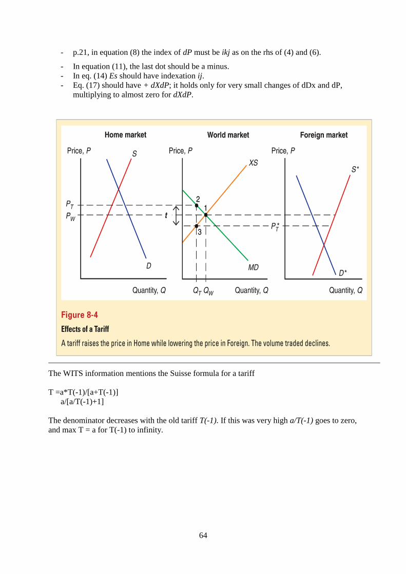
64

- p.21, in equation (8) the index of dP must be ikj as on the rhs of (4) and (6).

- In equation (11), the last dot should be a minus.

- In eq. (14) Es should have indexation ij.

- Eq. (17) should have + dXdP; it holds only for very small changes of dDx and dP,

multiplying to almost zero for dXdP.

The WITS information mentions the Suisse formula for a tariff

T =a*T(-1)/[a+T(-1)]

a/[a/T(-1)+1]

The denominator decreases with the old tariff T(-1). If this was very high a/T(-1) goes to zero,

and max T = a for T(-1) to infinity.