task2 modelingissues spear - fenixedurbento/tmp/3disp/task2... · 2012-11-05 · 6 3.2...
TRANSCRIPT

ISSN: 0871-7869
Influence of Modelling Issues on Nonlinear
Seismic Analysis of SPEAR Building
A. Belejo; R. Bento
- Novembro de 2012 -
Relatório ICIST DTC nº 21/2012

2
LIST!OF!CONTENTS!
LIST OF CONTENTS .................................................................................................................... 2!
1! INTRODUCTION .................................................................................................................... 3!
2! CASE STUDY – SPEAR BUILDING ....................................................................................... 3!
3! MODELLING ISSUES ............................................................................................................. 5!
3.1! Original model .................................................................................................................. 5!
3.2! Modelling changes proposed ........................................................................................... 6!
3.2.1! Consideration of 2% tangent stiffness-proportional damping (AN_D) ....................... 6!
3.2.2! Elasticity Modulus reduction of Reinforcement Steel (AN_E) .................................... 6!
3.2.3! Increase of the Elements’ length (AN_L) ................................................................... 6!
3.2.4! Uniform mass distribution (AN_M) ............................................................................. 7!
4! COMPARISON OF RESULTS TAKING ACCOUNT ALL PROPOSALS (EXPERIMENT
(EXP) VS ANALYTICAL MODEL) ................................................................................................. 8!
4.1! Dynamic Characteristics ................................................................................................... 8!
4.2! Top Displacements ........................................................................................................... 9!
5! CONCLUSIONS .................................................................................................................... 26!
ACKNOWLEDGMENTS .............................................................................................................. 28!
REFERENCES ............................................................................................................................ 29!
! !

3
1 INTRODUCTION!
In the scope of the research project PTDC/ECM/100299/2008 (www.3disp.org), and as far as
Task 2 is concerned (evaluate the influence of modelling issues on nonlinear seismic static
analysis of 3D irregular structures), some changes in the model of SPEAR building are
proposed to take into account some modelling aspects not considered previously (e.g. Bento et
al., 2009), aiming the approximation between experimental and analytical results.
The well-known SPEAR building has been tested in terms of seismic behaviour due its plan
irregularity. It was built to full-scale and tested within the European project SPEAR (Fardis and
Negro, 2006) to represent typical old constructions that do not have any specific provisions for
earthquake resistance. It was tested in ELSA lab with a bidirectional loading in three runs of
increasing amplitude (0.02g, 0.15g and 0.20g) based on a record obtained in Hercegnovi during
1979 Montenegro earthquake and fitted the EC8 spectrum, type 1 and Soil C (CEN, 2004).
In 2008, in the scope of the International Workshop on Nonlinear Static Methods for
Design/Assessment of 3D structures in Lisbon, the seismic assessment of the SPEAR Building
(Bento et al., 2009) was performed by means of some nonlinear static procedures and nonlinear
dynamic analyses. The model of the SPEAR building considered was validated comparing the
numerical results with the experimental ones obtained through the pseudo-dynamically tested
(Fardis and Negro, 2006).
The results of top displacements and interstorey drifts obtained over time for an intensity of
0.20g are displayed in Bhatt (2012) and Bento et al. (2009). At that time, the main objective of
the work was to compare different type of nonlinear static procedures, and not reproducing
completely the experimental behaviour. Therefore, some modelling aspects were not fully
considered. Currently, so some changes in the analytical model are performed in order to model
the building as close as possible to the one experimentally tested.
2 CASE!STUDY!–!SPEAR!BUILDING!
The heights of the storeys are 2.75 m for the first floor and 3.00 m for the upper storeys. The
building features a non-symmetrical plan configuration but is regular in elevation (Figure 2.1).
Only one column (C6) presents a rectangular section of 250×750 mm. All the others have a
square cross-section of 250×250 mm. The column C6 and the presence of a balcony on the
east side of the structure are the causes for the in-plan irregularity, shifting the centre of mass
away from the centre of stiffness, which is very close to the central column (C3).

4
a) b)
Figure 2.1 – SPEAR building: a) Plan view (m); b) Lateral view (m) (Bhatt, 2012)
Figure 2.2 – The full-scale SPEAR Building (Fardis et al, 2006)
The concrete is considered unconfined, due to the almost inexistent transversal reinforcement,
and a mean compressive strength of 25 MPa was assumed. Average yield strength of 360 MPa
and an ultimate strength of 450 MPa were considered for reinforcement steel.
Total translational masses, obtained from the seismic combination, amounted to 67.3 tonnes
each for the first two floors and 62.8 tonnes for the roof.

5
3 MODELLING!ISSUES!
3.1 Original!model!
The software used in the modelling of SPEAR building was SeismoStruct (SeismoSoft, 2011) a
fibre-based structural program. The building was modelled by an assemblage of inter-connected
frame elements using distributed material inelasticity through displacement-based formulation
along with geometric nonlinearity.
Each element was discretized into four sub-elements with two integration points each. Fiberized
cross-sections − representing sectional details such as cover and core concrete and longitudinal
reinforcements − were then defined at respective integration points, whereby every fibre was
assigned to an appropriate material constitutive relationship.
The constitutive relationship proposed by Mander et al. (1988) was deployed to model the
behaviour of unconfined concrete. In absence of sufficient transverse reinforcement, the
confinement effects were not considered for core concrete. The constitutive model used for the
steel was proposed by Menegotto and Pinto (1973) including the modifications due to isotropic
hardening proposed by Filippou et al. (1983).
A lumped mass modelling strategy was adopted, in which masses were lumped at the nodal
points according to its tributary area and by means of the defined masses; the software
automatically computed the sustained gravity loads.
The floor slabs of the building possessed very high in-plane stiffness compared to the out-of-
plane one; therefore these elements can safely be modelled$ as ‘rigid diaphragm’. The rigid
diaphragm effect was modelled by means of Lagrange Multipliers.
The results displayed in Bhatt (2012) and Bento et al. (2009) in terms of comparison between
analytical model and experimental test were obtained considering 0% of damping introduced.
However this model issue was reviewed after and a 2% tangent stiffness-proportional damping
was introduced to account for possible non-hysteretic sources of damping during analyses.
However some modelling aspects in the work presented in (Bhatt, 2012; Bento et al., 2009)
were not considered like beam-column joints, slippage and pullout of smooth reinforced bars,
strain penetration length, etc. Thus new modelling features are proposed to take account the
most of these aspects to improve the results, taking as reference the experimental results
(Fardis and Negro, 2006).

6
3.2 Modelling!changes!proposed!!
Firstly, some changes in the model were applied (one by one) and the results obtained
compared with the ones from model used in (Bento et al. 2009) (AN) and the experimental
results. Some of the changing options adopted were enabled to improve the results, i.e.
minimize the differences between the results of analytical model and experimental test. The
ones, which lead to better results, were selected and then combined to obtain the best result
possible.
In the following, the different modelling options adopted are described.
3.2.1 Consideration of 2% tangent stiffness-proportional damping (AN_D)
As it was previously mentioned, a 2% tangent stiffness-proportional damping was considered to
account for possible non-hysteretic sources of damping during analyses. So for this reason, a
2% tangent stiffness-proportional damping was also introduced.
3.2.2 Elasticity Modulus reduction of Reinforcement Steel (AN_E)
Stiffness reduction of the reinforcement steel is a pragmatic option to consider the slippage and
the pullout of smooth reinforced bars (Pinho, 2012); since there is not certain if the
reinforcement bars are folded in the ends of the elements. In other hand, ignoring the strain
penetration in nonlinear analyses of concrete structures will overestimate the stiffness,
hysteretic energy dissipation capacities, strains and section curvature (Zhao and Sritharan,
2007). Therefore to try to overcome these conditionings, the Elasticity Modulus of reinforcement
steel is reduced in 25%.
3.2.3 Increase of the Elements’ length (AN_L)
The increase of the elements length is an alternative to try to get the nonlinear behaviour for the
joints and in other hand to consider the penetration strain length, once ignoring the strain
penetration will underestimate the deflections and member elongation. Usually this feature is
considered adding this length to the plastic hinge length (Harn et al, 2010). However in this case
one are dealing with a fibre-based model where distributed material inelasticity is associated to
the elements. For fibre-based elements Ian Zhao and Sri Sritharan (2007) proposed a method
which introduces a hysteretic model for the reinforcing bar stress vs. slip response that can be
integrated into fibre-based analysis of concrete structures using a zero-length section element,
applicable in OpenSEES (PEER, 2006).

7
This option, of increasing the element length, was applied in two different ways: increasing only
0.10 m the length of each column (AN_L); and increasing 0.10 m the length of the beams
connected with external columns (all) and in the last storey columns (AN_L’).
3.2.4 Uniform mass distribution (AN_M)
Lumped masses were defined in the columns nodes. To define the masses in each column, the
axial forces of a distributed loading were obtained to get the percentage of force in each one.
This option was considered because the distribution of water tanks was determined by locating
their centre of weight at the centre of weight of slabs (Figure 3.1) to give the same axial force on
columns as the uniform load distribution (Jeong and Elnashai, 2005).
a) b)
Figure 3.1 - Weight determination: (a) Water tank location, (b) Comparison of axial forces on the first story
columns between water tank gravity load and uniformly distributed gravity load (Jeong and Elnashai, 2005)

8
4 COMPARISON!OF!RESULTS!TAKING!ACCOUNT!ALL!PROPOSALS!
(EXPERIMENT!(EXP)!VS!ANALYTICAL!MODEL)!!
The results herein compared are top displacements and interstorey drifts in nodes C1 and C7
for x direction and nodes N1 and C9 for y direction (Figure 2.1). Also the dynamic
characteristics of the structure are compared though knowing that the periods of vibration of the
specimen experiment will keep being higher and it is explained due to the reduction of stiffness
caused by the cracking in the columns, occurring when the test specimen was transported from
outside the ELSA lab, where it was built, into the inside of the laboratory, where it was tested.
For all analytical models, all analyses were performed considering the rigid diaphragm effect
modelled by means of Penalty Functions (exponent 107) instead of Lagrange Multipliers.
Otherwise it would be impractical to perform so many analyses as required.
All the results herein obtained are displayed in percentage, relative to the maximum
experimental results. In the following table the maximum results obtained in the experimental
test in terms of top displacements and interstorey drifts in x and y direction respectively are
shown.
Table 4.1 – Maximum results obtained in the experimental test for x direction
Node Max Top
Displacement
Maximum Interstorey Drift
0-1st storey 1st-2nd storey 2nd-3rd storey
C7 114.82 mm 31.6 mm 62.6 mm 34.4 mm
C1 133.08 mm 38.0 mm 72.8 mm 63.6 mm
Table 4.2 - Maximum results obtained in the experimental test for y direction
Node Max Top
Displacement
Maximum Interstorey Drift
0-1st storey 1st-2nd storey 2nd-3rd storey
N1 165.17 mm 40.9 mm 80.2 mm 60.2 mm
C9 115.62 mm 30.1 mm 56.8 mm 42.6 mm
4.1 Dynamic!Characteristics!
In Table 4.3 the first and second periods of vibration of the structure are presented for the
alternatives mentioned before. The results presented show that the introduction of stiffness-

9
proportional damping does not cause any difference in the first periods of vibration in the
structure. From all the other options, there are small differences, but all of them still far from the
values obtained with the experimental specimen, as was expected.
Table 4.3 – First Periods of Vibration of the structure of experimental test and analytical models
considering only the change in the models
Case T1 (s) T2 (s) EXP 0.85 0.78 AN 0.62 0.53
AN_D 0.62 0.53 AN_E 0.63 0.53 AN_L 0.65 0.55 AN_L' 0.62 0.55 AN_M 0.62 0.54
Combining these modelling changes, the results obtained are displayed in Table 4.4. In this
table are presented the results of the several modelling changes combined: Elasticity Modulus
reduction of Reinforcement Steel and Increase of the Elements’ length (AN_LE), Elasticity
Modulus reduction and Uniform mass distribution (AN_ME), Increase of the Elements’ length
and Uniform mass distribution (AN_ML) and the combination of these three already mentioned
(AN_MLE). Based on these results obtained one can say that by combining all these changes
the results get slighter closer to the results from experimental test.
In these combinations, and as far as the increase of elements length concerns, only the increase of the columns was considered. In next sections is shown that this alternative gets equal or better results than the increase of the beams and last storey columns.
Table 4.4 - First Periods of Vibration of the structure of experimental test and analytical models
considering combined changes in the models
Case T1 (s) T2 (s) EXP 0.85 0.78 AN 0.62 0.53
AN_LE 0.66 0.56 AN_ME 0.63 0.54 AN_ML 0.66 0.56
AN_MLE 0.66 0.57
4.2 Top!Displacements!
The top displacements obtained by Bento et al. (2009) for a seismic intensity of 0.20g are
displayed in the figures 4.1 and 4.2.

10
a) b)
Figure 4.1 – EXP & AN - Top Displacements in x direction: a) node C7; b) node C1
a) b)
Figure 4.2 - EXP & AN - Top Displacements in y direction: a) node N1; b) node C9
These displacement profiles, represented with the thin line, should be improved in order to
obtain the closest possible to the gross line profiles.
Analysing the different approaches taking account the changes referred one by one, the
displacements profiles in the same nodes and corresponding to the same directions are
obtained and displayed in the following figures.
Introducing of 2% tangent stiffness-proportional damping
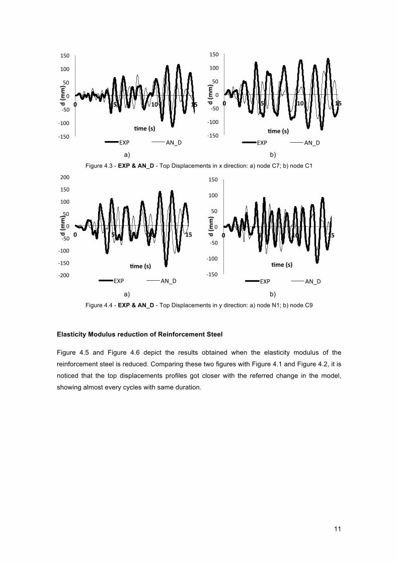
In terms of top displacements, can be seen by Figure 4.3 and Figure 4.4 that the introduction of
damping does not improve the results, so all the remaining analyses are made with no damping.
"150!
"100!
"50!
0!
50!
100!
150!
0" 5" 10" 15"d"(m
m)"
)me"(s)"
EXP! AN!
"150!
"100!
"50!
0!
50!
100!
150!
0" 5" 10" 15"
d"(m
m)"
)me"(s)""
EXP! AN!
"200!
"150!
"100!
"50!
0!
50!
100!
150!
200!
0" 5" 10" 15"
d"(m
m)"
)me"(s)"
EXP! AN!
"150!
"100!
"50!
0!
50!
100!
150!
0" 5" 10" 15"d"(m
m)"
)me"(s)"
EXP! AN!
11
a) b)
Figure 4.3 - EXP & AN_D - Top Displacements in x direction: a) node C7; b) node C1
a) b)
Figure 4.4 - EXP & AN_D - Top Displacements in y direction: a) node N1; b) node C9
Elasticity Modulus reduction of Reinforcement Steel
Figure 4.5 and Figure 4.6 depict the results obtained when the elasticity modulus of the
reinforcement steel is reduced. Comparing these two figures with Figure 4.1 and Figure 4.2, it is
noticed that the top displacements profiles got closer with the referred change in the model,
showing almost every cycles with same duration.
"150!
"100!
"50!
0!
50!
100!
150!
0" 5" 10" 15"d"(m
m)"
)me"(s)"
EXP! AN_D!"150!
"100!
"50!
0!
50!
100!
150!
0" 5" 10" 15"d"(m
m)"
)me"(s)"
EXP! AN_D!
"200!
"150!
"100!
"50!
0!
50!
100!
150!
200!
0" 5" 10" 15"d"(m
m)"
)me"(s)"
EXP! AN_D!"150!
"100!
"50!
0!
50!
100!
150!
0" 5" 10" 15"d"(m
m)"
)me"(s)"
EXP! AN_D!

12
a) b)
Figure 4.5 - EXP & AN_E - Top Displacements in x direction: a) node C7; b) node C1
a) b)
Figure 4.6 - EXP & AN_E - Top Displacements in y direction: a) node N1; b) node C9
Increase of the Elements’ length
The results herein presented show that this option also improves the results. However the
differences between the two approaches described are not evident in any case. However in
terms of mean and maximum differences, the option that considers only the increase of the
length of the columns show better approximation to the experimental test as can be seen in
Table 4.5.
"150!
"100!
"50!
0!
50!
100!
150!
0" 5" 10" 15"d"(m
m)"
)me"(s)"EXP! AN_E!
"150!
"100!
"50!
0!
50!
100!
150!
0" 5" 10" 15"d"(m
m)"
)me"(s)"
EXP! AN_E!
"200!
"150!
"100!
"50!
0!
50!
100!
150!
200!
0! 5! 10! 15!d"(m
m)"
)me"(s)"EXP! AN_E!
"150!
"100!
"50!
0!
50!
100!
150!
0" 5" 10" 15"d"(m
m)"
)me"(s)"
EXP! AN_E!

13
a) b)
Figure 4.7 – EXP, AN_L & AN_L’ - Top Displacements in x direction: a) node C7; b) node C1
a) b)
Figure 4.8 - EXP, AN_L & AN_L’ - Top Displacements in y direction: a) node N1; b) node C9
Table 4.5 - Top displacements differences between Experimental test and Analytical models
Case
Mean difference Maximum
difference Mean difference
Maximum
difference
x direction y direction
C7 C1 C7 C1 N1 C9 N1 C9
AN 24% 41% 71% 109% 27% 26% 87% 78%
AN_L 20% 39% 60% 104% 25% 23% 77% 73%
AN_L’ 24% 41% 68% 108% 27% 25% 84% 79%
Uniform mass distribution
With the different mass distribution assumed in this study, it is observed that generally the
displacements profile has a better match with the experimental test profile.
"150!
"100!
"50!
0!
50!
100!
150!
0" 5" 10" 15"d"(m
m)"
)me"(s)"EXP! AN_L! AN_L'! "150!
"100!
"50!
0!
50!
100!
150!
0" 5" 10" 15"d"(m
m)"
)me"(s)"EXP! AN_L! AN_L'!
"200!
"150!
"100!
"50!
0!
50!
100!
150!
200!
0" 5" 10" 15"d"(m
m)"
)me(s)"EXP! AN_L! AN_L'!
"150!
"100!
"50!
0!
50!
100!
150!
0! 5! 10! 15!d"(m
m)"
)me"(s)"EXP! AN_L! AN_L'!

14
a) b)
Figure 4.9 – EXP & AN_M - Top Displacements in x direction: a) node C7; b) node C1
a) b)
Figure 4.10 – EXP & AN_M - Top Displacements in y direction: a) node N1; b) node C9
In the following tables there is a summary describing the mean and maximum difference
between experimental test and analytical models and still difference between maximum
displacements and respective error in the x and y directions respectively.
Table 4.6 –Top displacements differences between Experimental test and Analytical models in x direction
Case Mean difference Maximum difference
Difference between
maximums
C7 C1 C7 C1 C7 C1
AN 24% 41% 71% 109% -2% -10%
AN_D 30% 45% 96% 138% -33% -32%
AN_E 20%** 38%** 59%** 107%* 13% -9%*
AN_L 20%* 39%* 60%* 104%** 6% -8%**
AN_M 24% 41%* 73% 112% 1%** -21%
* Closer to experimental test results than reference (bold) results ** Closest to experimental test results
"150!
"100!
"50!
0!
50!
100!
150!
0! 5! 10! 15!d"(m
m)"
)me"(s)"
EXP! AN_M!"150!
"100!
"50!
0!
50!
100!
150!
0! 5! 10! 15!d"(m
m)"
)me"(S)"EXP! AN_M!
"200!
"150!
"100!
"50!
0!
50!
100!
150!
200!
0" 5" 10" 15"d"(m
m)"
)me"(s)"
EXP! AN_M!"150!
"100!
"50!
0!
50!
100!
150!
0! 5! 10! 15!d"(m
m)"
)me"(s)"
EXP! AN_M!

15
Table 4.7 - Top displacements differences between Experimental test and Analytical models in y direction
Case Mean difference Maximum difference
Difference between
maximums
N1 C9 N1 C9 N1 C9
AN 27% 26% 87% 78% -33% -25%
AN_D 31% 27% 117% 70%** -32%* -38%
AN_E 24%** 23%* 73%** 72%* -25%** -1%**
AN_L 25%* 23%** 77%* 73%* -31%* -22%*
AN_M 26%* 28% 83%* 83% -36% -21%*
* Closer to experimental test results than reference (bold) results ** Closest to experimental test results
From the analysis of the top displacements profiles, Table 4.6 and Table 4.7 show that the
changes applied to the model related with stiffness reduction, elements’ increase and uniform
mass distribution are able to improve the results and obtain closer results to the experimental
test comparing to the model used in (Bento et al., 2009).
Therefore the results herein obtained suggest to combine these approaches to get even better
match with experimental test.
So, in the following, the top displacements profiles in the same points and for the directions
considered previously are shown, combining the different approaches already studied resulting
in other four different approaches (the same already used to obtain the first periods of the
structure in Chapter 4.1)
Elasticity Modulus reduction of Reinforcement Steel and Increase of the Elements’ length
a) b)
Figure 4.11 – EXP & AN_LE - Top Displacements in x direction: a) node C7; b) node C1
"150!
"100!
"50!
0!
50!
100!
150!
0" 5" 10" 15"d"(m
m)"
)me"(s)"
EXP! AN_LE! "150!
"100!
"50!
0!
50!
100!
150!
0! 5! 10! 15!d"(m
m)"
)me"(s)"
EXP! AN_LE!

16
a) b)
Figure 4.12 – EXP & AN_LE - Top Displacements in y direction: a) node N1; b) node C9
Elasticity Modulus reduction of Reinforcement Steel and Uniform mass distribution
a) b)
Figure 4.13 – EXP & AN_ME - Top Displacements in x direction: a) node C7; b) node C1
a) b)
Figure 4.14 – EXP & AN_ME - Top Displacements in y direction: a) node N1; b) node C9
"200!
"150!
"100!
"50!
0!
50!
100!
150!
200!
0" 5" 10" 15"d"(m
m)"
)me"(s)"
EXP! AN_LE!"150!
"100!
"50!
0!
50!
100!
150!
0" 5" 10" 15"d"(m
m)"
)me"(s)"EXP! AN_LE!
"150!
"100!
"50!
0!
50!
100!
150!
0! 5! 10! 15!d"(m
m)"
)me"(s)"
EXP! AN_ME!"150!
"100!
"50!
0!
50!
100!
150!
0! 5! 10! 15!d"(m
m)"
)me"(s)"
EXP! AN_ME!
"200!
"150!
"100!
"50!
0!
50!
100!
150!
200!
0" 5" 10" 15"d"(m
m)"
)me""(s)"EXP! AN_ME! "150!
"100!
"50!
0!
50!
100!
150!
0" 5" 10" 15"d"(m
m)"
)me"(s)"
EXP! AN_ME!

17
Increase of the Elements’ length and Uniform mass distribution
a) b)
Figure 4.15 – EXP & AN_ML - Top Displacements in x direction: a) node C7; b) node C1
a) b)
Figure 4.16 – EXP & AN_ML - Top Displacements in y direction: a) node N1; b) node C9
Elasticity Modulus reduction of Reinforcement Steel, Increase of the Elements’ length
and Uniform mass distribution
a) b)
Figure 4.17 – EXP & AN_MLE - Top Displacements in x direction: a) node C7; b) node C1
"150!
"100!
"50!
0!
50!
100!
150!
0" 5" 10" 15"d"(m
m)"
)me"(s)"EXP! AN_ML!
"150!
"100!
"50!
0!
50!
100!
150!
0" 5" 10" 15"d"(m
m)"
)me"(s)"
EXP! AN_ML!
"200!
"150!
"100!
"50!
0!
50!
100!
150!
200!
0! 5! 10! 15!d"(m
m)"
)me"(s)"
EXP! AN_ML!"150!
"100!
"50!
0!
50!
100!
150!
0! 5! 10! 15!d"(m
m)"
)me"(s)"
EXP! AN_ML!
"200!
"150!
"100!
"50!
0!
50!
100!
150!
0" 5" 10" 15"d"(m
m)"
)me"(s)"
EXP! AN_MLE!"150!
"100!
"50!
0!
50!
100!
150!
0! 5! 10! 15!d"(m
m)"
)me"(s)"
EXP! AN_MLE!

18
a) b)
Figure 4.18 – EXP & AN_MLE - Top Displacements in y direction: a) node N1; b) node C9
The results in terms of differences between experimental test and analytical models are
presented in Table 4.8 and Table 4.9. The reference values herein presented, showed in bold,
correspond to the minimum values obtained by the approaches, which consider only one
change in the model.
Table 4.8 –Top displacements differences between Experimental test and Analytical models in x direction
including combined approaches
Case Mean difference Maximum difference
Difference between
maximums
C7 C1 C7 C1 C7 C1
AN 24% 41% 71% 109% -2% -10%
AN_D 30% 45% 96% 138% -33% -32%
AN_E 20% 38% 59% 107% 13% -9%
AN_L 20% 39% 60% 104% 6% -8%
AN_M 24% 41% 73% 112% 1% -21%
AN_LE 18%** 33%* 56%** 90%* 13% -28%
AN_ME 19%* 37%* 61% 113% 8% -18%
AN_ML 20% 39% 65% 108% 22% -22%
AN_MLE 18%* 30%** 67% 88%** 4% -18%
* Closer to experimental test results than reference (bold) results ** Closest to experimental test results
"200!
"150!
"100!
"50!
0!
50!
100!
150!
200!
0! 5! 10! 15!d(mm)"
)me"(s)"
EXP! AN_MLE!"150!
"100!
"50!
0!
50!
100!
150!
0! 5! 10! 15!d"(m
m)"
)me"(s)"EXP! AN_MLE!

19
Table 4.9 - Top displacements differences between Experimental test and Analytical models in y direction
including combined approaches
Case Mean difference Maximum difference
Difference between
maximums
N1 C9 N1 C9 N1 C9
AN 27% 26% 87% 78% -33% -25%
AN_D 31% 27% 117% 70% -32% -38%
AN_E 24% 23% 73% 72% -25% -1%
AN_L 25% 23% 77% 73% -31% -22%
AN_M 26% 28% 83% 84% -36% -21%
AN_LE 22%* 22%* 64%* 75% -23%** 9%
AN_ME 24%* 25% 71%* 79% -25%* -1%*
AN_ML 25% 25% 77% 79% -27% 0%**
AN_MLE 21%** 21%** 63%** 65%** -32% -19%
* Closer to experimental test results than reference (bold) results ** Closest to experimental test results
Considering these new approaches, where were combined the suggested changes in the
models, is verified that the results in terms of top displacements were still improved. The mean
difference between top displacements was reduced in some nodes comparing with the “best”
results obtained before.
When all changes proposed in the model are combined (except damping addiction), all
differences of displacements obtained for both directions are reduced due the good match
between top displacements profiles (experimental and analytical). In three nodes, of four
analysed, mean and maximum differences are the smallest for this approach.
In Table 4.8 and Table 4.9, the maximum values of the displacements in experimental and
analytical analyses are showed, and only in node C7 the analytical test overestimates the
displacements for all approaches. In the other nodes top displacements are generally lower
compared with experimental test, however with the changes performed in the model, the
differences become smaller, getting close to the experimental values.
Interstorey Drifts
To study the structure behaviour of the other stories, also the interstorey drifts were calculated
using the analytical model considering the changes mentioned before and the experimental test.
So can be verified the influence of the proposed changes in the model for all structure.
The interstorey drifts obtained by Bento et al. (2009) for a seismic intensity of 0.20g are
displayed in the Figure 4.19 for the 1st-2nd floor in the x direction and for first floor in y direction
for nodes C7 and C9 respectively.

20
a) b)
Figure 4.19 – EXP & AN – Interstorey drifts: a) 1st storey drifts at node C7 in x direction: a) 1st-2nd stories
at node C9 in y direction
The modelling changes, herein considered, are the same, which were applied to obtain the top
displacements as well as the combinations performed.
So in the following figures the first floor interstorey drifts in node C9 in y direction and 1st-2nd
floors interstorey drifts in node C7 for x direction, are shown considering the referred
approaches excluding the model with damping since it shows worst result for top
displacements.
Elasticity Modulus reduction of Reinforcement Steel
Figure 4.20 – EXP & AN_E – Interstorey drifts: a) 1st storey drifts at node C7 in x direction: a) 1st-2nd
stories at node C9 in y direction
"60!
"40!
"20!
0!
20!
40!
60!
80!
0" 5" 10" 15"id"(m
m)"
)me"(s)"EXP! AN! "40!
"30!
"20!
"10!
0!
10!
20!
30!
0! 5! 10! 15!
d"(m
m)"
)me"(s)"
EXP! AN!
a) b)
"60!
"40!
"20!
0!
20!
40!
60!
80!
0! 5! 10! 15!
id"(m
m)"
)me"(s)"
EXP! AN_E!
"50!"40!"30!"20!"10!0!
10!20!30!40!50!
0! 5! 10! 15!id"(m
m)"
)me"(s)"EXP! AN_E!
21
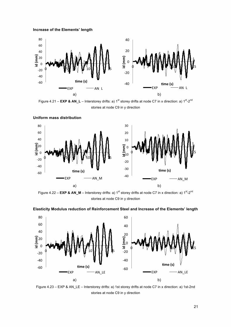
Increase of the Elements’ length
Figure 4.21 – EXP & AN_L – Interstorey drifts: a) 1st storey drifts at node C7 in x direction: a) 1st-2nd
stories at node C9 in y direction
Uniform mass distribution
Figure 4.22 – EXP & AN_M – Interstorey drifts: a) 1st storey drifts at node C7 in x direction: a) 1st-2nd
stories at node C9 in y direction
Elasticity Modulus reduction of Reinforcement Steel and Increase of the Elements’ length
Figure 4.23 – EXP & AN_LE – Interstorey drifts: a) 1st storey drifts at node C7 in x direction: a) 1st-2nd
stories at node C9 in y direction
a) b)
a) b)
a) b)
"60!
"40!
"20!
0!
20!
40!
60!
80!
0! 5! 10! 15!
id"(m
m)"
)me"(s)"
EXP! AN_L!"40!
"20!
0!
20!
40!
0! 5! 10! 15!id"(m
m)"
)me"(s)"EXP! AN_L!
"60!
"40!
"20!
0!
20!
40!
60!
80!
0! 5! 10! 15!
id"(m
m)"
)me"(s)"
EXP! AN_M! "40!
"30!
"20!
"10!
0!
10!
20!
30!
0! 5! 10! 15!
id"(m
m)"
)me"(s)"
EXP! AN_M!
"60!
"40!
"20!
0!
20!
40!
60!
80!
0! 5! 10! 15!
id"(m
m)"
)me"(s)"EXP! AN_LE!
"60!
"40!
"20!
0!
20!
40!
60!
0! 5! 10! 15!id"(m
m)"
)me"(s)"
EXP! AN_LE!
22
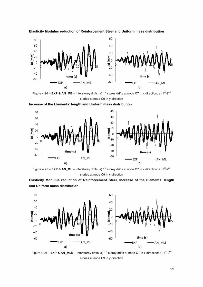
Elasticity Modulus reduction of Reinforcement Steel and Uniform mass distribution
Figure 4.24 – EXP & AN_ME – Interstorey drifts: a) 1st storey drifts at node C7 in x direction: a) 1st-2nd
stories at node C9 in y direction
Increase of the Elements’ length and Uniform mass distribution
Figure 4.25 – EXP & AN_ML – Interstorey drifts: a) 1st storey drifts at node C7 in x direction: a) 1st-2nd
stories at node C9 in y direction
Elasticity Modulus reduction of Reinforcement Steel, Increase of the Elements’ length
and Uniform mass distribution
Figure 4.26 – EXP & AN_MLE – Interstorey drifts: a) 1st storey drifts at node C7 in x direction: a) 1st-2nd
stories at node C9 in y direction
a) b)
a) b)
a) b)
"60!
"40!
"20!
0!
20!
40!
60!
80!
0! 5! 10! 15!
id"(m
m)"
)me"(s)"
EXP! AN_ME! "60!
"40!
"20!
0!
20!
40!
60!
0! 5! 10! 15!id"(m
m)"
)me"(s)"
EXP! AN_ME!
"60!
"40!
"20!
0!
20!
40!
60!
80!
0! 5! 10! 15!
id"(m
m)"
)me"(s)"
EXP! AN_ML! "40!
"30!
"20!
"10!
0!
10!
20!
30!
40!
0! 5! 10! 15!id"(m
m)"
)me"(s)"
EXP! AN_ML!
"60!
"40!
"20!
0!
20!
40!
60!
80!
0! 5! 10! 15!
id"(m
m)"
)me"(s)"
EXP! AN_MLE!"60!
"40!
"20!
0!
20!
40!
60!
0! 5! 10! 15!id"(m
m)"
)me"(s)"EXP! AN_MLE!

23
From the interstorey drifts profiles, one can conclude that, in most of the cases, there is a very
reasonable match between interstorey drifts profiles, improving the results obtained before
changing the model. The only exception occurs with the analytical model considering a uniform
mass distribution, as can be seen in Figure 4.22.
From the observation of the interstorey drifts profiles can be noticed that for 1st storey the
interstorey drifts are overestimated and on other hand, for 1st-2nd storey they are
underestimated. However, additional conclusions could be achieved with the observation of
Table 4.10 and Table 4.11.
The follow tables show a resume of all interstorey drifts in the four columns considered in each
floor (C7 and C1 for x direction and N1 and C9 for y direction).
Table 4.10 – Interstorey Drifts differences between Experimental test and Analytical models in x direction
Case Stories Mean difference Maximum difference Difference between
maximum displacements
C7 C1 C7 C1 C7 C1 AN
0-1st
28% 38% 104% 166% 44% -28%
AN_E 30% 36%* 137% 166% 52% 15%*
AN_L 28% 36%* 119% 164%* 49% -11%**
AN_M 29% 37%* 107% 143%* 48% 45%
AN_LE 32% 29%* 172% 102%** 55% 27%
AN_ME 30% 34%* 146% 153%* 55% 48%
AN_ML 29% 35%* 119% 141%* 53% 45%
AN_MLE 33% 27%** 171% 107%* 52% 19%*
AN
1st –
2nd
22% 34% 69% 93% -30% -46%
AN_E 18%* 32%* 49%** 77%* -19%** -42%*
AN_L 19%* 33%* 62%* 84%* -26%* -46%*
AN_M 22% 34%* 73% 88%* -27%* -51%
AN_LE 14%* 29%* 59%* 72%* -28%* -35%**
AN_ME 17%* 32%* 56%* 80%* -25%* -51%
AN_ML 19%* 33%* 67%* 79%* -28%* -53%
AN_MLE 14%** 28%** 70% 67%** -24%* -45%*
AN
2nd –
3rd
30% 33% 97% 126% -4% -54%
AN_E 25%* 32%* 72%* 123%* 16% -52%*
AN_L 25%* 32%* 78%* 122%* 3%** -54%
AN_M 30% 34% 100% 129% -8% -37%*
AN_LE 20% 30%* 67%* 103%** 17% -49%*
AN_ME 25%* 32%* 80%* 131% 20% -31%**
AN_ML 26%* 32%* 81%* 127% 9% -39%*
AN_MLE 19%** 30%** 63%** 103%* 15% -44%* * Closer to experimental test results than reference (bold) results ** Closest to experimental test results

24
Table 4.11 - Interstorey Drifts differences between Experimental test and Analytical models in y direction
Case Stories Mean difference Maximum
difference
Difference between
maximum displacements
N1 C9 N1 C9 N1 C9
AN 0-
1st
26% 23% 113% 83% 29% 62%
AN_E 25%* 25% 109%* 80%* 30% 62%*
AN_L 25%* 23%** 101%* 78%** 27%* 61%*
AN_M 25%* 25% 99%* 90%* 21%* -2%**
AN_LE 22%* 27% 87 %* 131%* 26%* 44%*
AN_ME 25%* 27% 103%* 87%* 32% 32%*
AN_ML 24%* 25% 92%* 86%* 25%* 12%*
AN_MLE 19%** 27% 83%** 100%* 9%** 37%*
AN
1st –
2nd
25% 24% 87% 72% -52% -41%
AN_E 23%* 21%* 70%* 63%** -49%* -43%
AN_L 24%* 21%* 81%* 66%* -50%* -45%
AN_M 25%* 25% 87%* 76% -56% -29%*
AN_LE 21%* 20%* 58%* 76% -36%** -36%*
AN_ME 24%* 22%* 72%* 65%* -50%* -25%*
AN_ML 24%* 22%* 81%* 68%* -52%* -28%*
AN_MLE 21%** 19%** 58%** 70%* -37%* -21%**
AN
2nd –
3rd
30% 26% 100% 90% -33% -4%
AN_E 28%* 22%* 92%* 80%* -25%* -6%
AN_L 28%* 23%* 90%* 78%* -26%* -11%
AN_M 29%* 27% 97%* 91% -36% -26%
AN_LE 26%** 19%** 83%* 79%* -23%** -14%
AN_ME 28%* 24%* 90%* 86%* -27%* -18%
AN_ML 28%* 25%* 92%* 82%* -29%* -22%
AN_MLE 26%* 19%* 79%** 75%** -28%* -21%
* Closer to experimental test results than reference (bold) results ** Closest to experimental test results
Based on the values presented Table 4.10 and Table 4.11, one can conclude that the approach
which considers uniform distribution of mass also leads to worst results in terms of mean
differences, however does not present significant differences. The same conclusion can be
stated for the approaches that the uniform mass distribution is combined with other changes in
the model. Nevertheless the approach that considers the three changes in model (i.e. uniform
mass distribution, Elasticity Modulus reduction of Reinforcement Steel and increase of the
elements’ length) generally shows the best results. The other approaches that does not
consider the uniform mass distribution, generally present improved results.

25
In terms of maximum displacements, all analytical models show different behaviour comparing
with the results from the experimental test. Although the differences between experimental and
analytical results had been reduced, the analytical models present the highest interstorey drifts
in the first floor, i.e. they overestimate the results. In the other hand, the results from
experimental test show the 1st-2nd-storey drift as the highest and for this case analytical models
lead to underestimated results. The same occurs in 2nd-3rd interstorey drift, nevertheless with
much smaller differences. It means that in 2nd and 3rd floor, the analytical models are not being
able to pick up to model what has been occurred in the experimental test. The reason can be
related with the damage in some local areas (columns, joints, etc.) of the structure, which could
be occurred when the test specimen was transported from outside the ELSA lab, into the inside
of the laboratory, as previously mentioned.

26
5 CONCLUSIONS!
The conclusions of this study are described having as reference, the experimental test
performed with a record obtained in Hercegnovi during 1979 Montenegro earthquake fitted to
EC8 spectrum (type 1 and soil C) considering a peak ground acceleration of 0.20g.
Five different changes in the original analytical model, previously explained, were performed to
take in account some modelling aspects not considered before. Into these five changes, two of
them were excluded based on the top displacements results obtained only with these individual
changes: 1- Introduction of damping and 2- increase of the length of the beams and last storey
columns. The analytical results considering the damping in the model showed the worst results
in terms of profiles matching and mean and maximum differences, when compared with
experimental test. The analytical model considering increase of the length of the beams and last
storey columns presented worst results when comparing with the one, which all columns were
increased. Thus, since both analytical models were performed to consider the same aspects,
only one was chosen to continue the study.
After excluded the two abovementioned models, the study continued with the analytical models
remained; they were combined becoming four more different analytical cases (considering
uniform mass distribution and elasticity modulus reduction, uniform mass distribution and
increase of columns length; elasticity modulus reduction and increase of columns length and the
three changes in the same model). Observing the top displacements results obtained from the
combined approaches it was verified that they are even better in terms of profiles and mean and
maximum differences. And the approach, which is closer to the experimental test results, is the
one considering the three changes simultaneously in the analytical model. The same
conclusions had already been taken, though with less significance, when the first periods of
vibration obtained were compared. In terms of maximum displacements, the changes in the
model were able to approximate the results to the results of the experimental test in same
nodes. However there is not a total agreement in the results between approaches, nodes or
directions in this study, i.e. it is not possible to identify a final model which leads to better
results, for all type of outcomes analysed.
As far as interstorey drifts concern, the results were obtained taking into account all the
analytical models, considering the modelling changes individually and combined, as previously
mentioned. The change performed, in the analytical models, related with mass distribution does
not have much influence in the interstorey drifts results. In opposite the other changes have
significant importance, yielding to a very reasonable match between experimental test and
analytical models interstorey drifts. Similarly, the results related with mean and maximum
differences were improved due these changes.
The analytical models are not getting the interstorey drifts obtained in the experimental test,
even showing soft storey problems in different storeys.

27
Taking in account the set of differences performed in the model, it is difficult to get closer than
the results herein presented given that the conditions of the experimental specimen are not
known in detail.
To conclude, the changes performed in the model to decrease the stiffness of the model, to
increase the elements and to have exactly the same distribution of mass presented in the test
are reasonable and valid choices to overcome the modelling problems described in this study,
which usually are not taking in account for seismic studies, though in some cases may be
relevant.

28
ACKNOWLEDGMENTS!
The authors would like to acknowledge the financial support of the Portuguese Foundation for
Science and Technology through the research project PTDC/ECM/100299/2008.
!

29
REFERENCES!
Bento, R. Pinho. (2009). 3D Pushover 2008 – Nonlinear Static Methods for Design Assessment
of 3D Structures. IST Press, http://www.3dpushover.org/
Bhatt C. (2012) Seismic Assessment of Existing Buildings Using Nonlinear Static Procedures
(NSPs) - A New 3D Pushover Procedure; Thesis specifically prepared to obtain the PhD Degree
in Civil Engineering; Technical University of Lisbon
CEN, Eurocode 8 (EC8) 2004: Design of structures for earthquake resistance. Part 1: general
rules, seismic actions and rules for buildings. EN 1998-1:2004 Comité Européen de
Normalisation, Brussels, Belgium.
Fardis M. N. and Negro P. (2006): SPEAR – Seismic performance assessment and
rehabilitation of existing buildings, Proceedings of the International Workshop on the SPEAR
Project, Ispra, Italy.
Filippou, F.C., Popov, E.P. and Bertero, V.V. (1983). Modelling of R/C joints under cyclic
excitations. J. Struct.Eng. 109(11), 2666-2684
Harn, Robert E., Mays, Timothy W. and Johnson Gayle S. (2010) - Proposed Seismic Detailing
Criteria for Piers and Wharves. Proceedings of Ports 2010: Building on the Past, Respecting the
Future.
Jeong S. H. and Elnashai A. S., (2005). Analytical assessment of a 3D full scale RC building
test. Proceedings of the International Workshop on the SPEAR Project, Ispra, Italy
Mander JB, Priestley MJN, Park R (1988) Theoretical stress–strain model for confined concrete.
ASCE J Struct Eng 114(8), 1804–1826.
Menegotto M. and Pinto P.E. (1973). Method of analysis for cyclically loaded RC plane frames
including changes in geometry and non-elastic behaviour of elements under combined normal
force and bending. International Association for Bridge and Structural Engineering, Symposium
on the Resistance and Ultimate Deformability of Structures anted on by well defined loads, 15-
22. Zurich, Switzerland
PEER, 2006 OpenSEES: Open System for Earthquake Engineering Simulation. Pacific
Earthquake Engineering Research Center, University of California, Berkeley, CA.
Pinho R, (2012) - Modelação Sísmica de Edifícios Irregulares B.A – Alguns Aspectos Críticos
Curso de Formação "Análise Estáticas Não Lineares (Análises Pushover) para o
dimensionamento e avaliação sísmica de estruturas". Slides, FUNDEC, IST, Lisbon, Portugal
SeismoSoft, 2011, “SeismoStruct – A computer program for static and dynamic nonlinear
analysis of framed structures“ available online from http://www.seismosoft.com.

30
Zhao, J., and S. Sritharan. (2007) - Modelling of strain penetration effects in fiber-based
analysis of reinforced concrete structures. ACI Structural Journal, 104(2), pp. 133-141
!