task planning and multi-agent systems
TRANSCRIPT

Parameter Estimation and Adaptive Control!
Robert Stengel! Robotics and Intelligent Systems MAE 345, !
Princeton University, 2017•! Parameter estimation
–! after the fact–! real time
•! Simultaneous Location and Mapping (SLAM)•! Reinforcement (“Q”) learning•! Gain scheduling•! Adaptive critic (DHADP)•! Failure-tolerant control
Copyright 2017 by Robert Stengel. All rights reserved. For educational use only.http://www.princeton.edu/~stengel/MAE345.html 1
Off-Line!(i.e., “after the fact”) Parameter Estimation!
2

Parameter-Dependent Linear System
xk+1 = !! p( )xk + "" p( )ukzk = Hxk + nk
Linear systems contains parameters
What if the parameter vector, p, is unknown?
3
Least-Square-Error Estimates of System Parameters
Trends and higher-degree curve-fittingMultivariate estimation
Identification of dynamic system parameters
Error “Cost” Function
4

LTI System with Unknown Parameters
Parameters to be identified from experimental data, pKnown input, uk, noisy measurements, xk, made at
discrete instants of time
5
xk+1 = !! p( )xk + "" p( )uk + ## p( )wk , x0 givenzk = Hxk + nk , k = 0,K
Error Cost Function for Parameter Identification
J = !! kTR!! k
k=0
K
" = zk # x̂k[ ]T R zk # x̂k[ ]k=0
K
"
Weighted-square error of difference between measurements and model’s estimates
zk : Measurement data setx̂k : Estimate propagated by sampled-data modelR : Weighting matrix
6
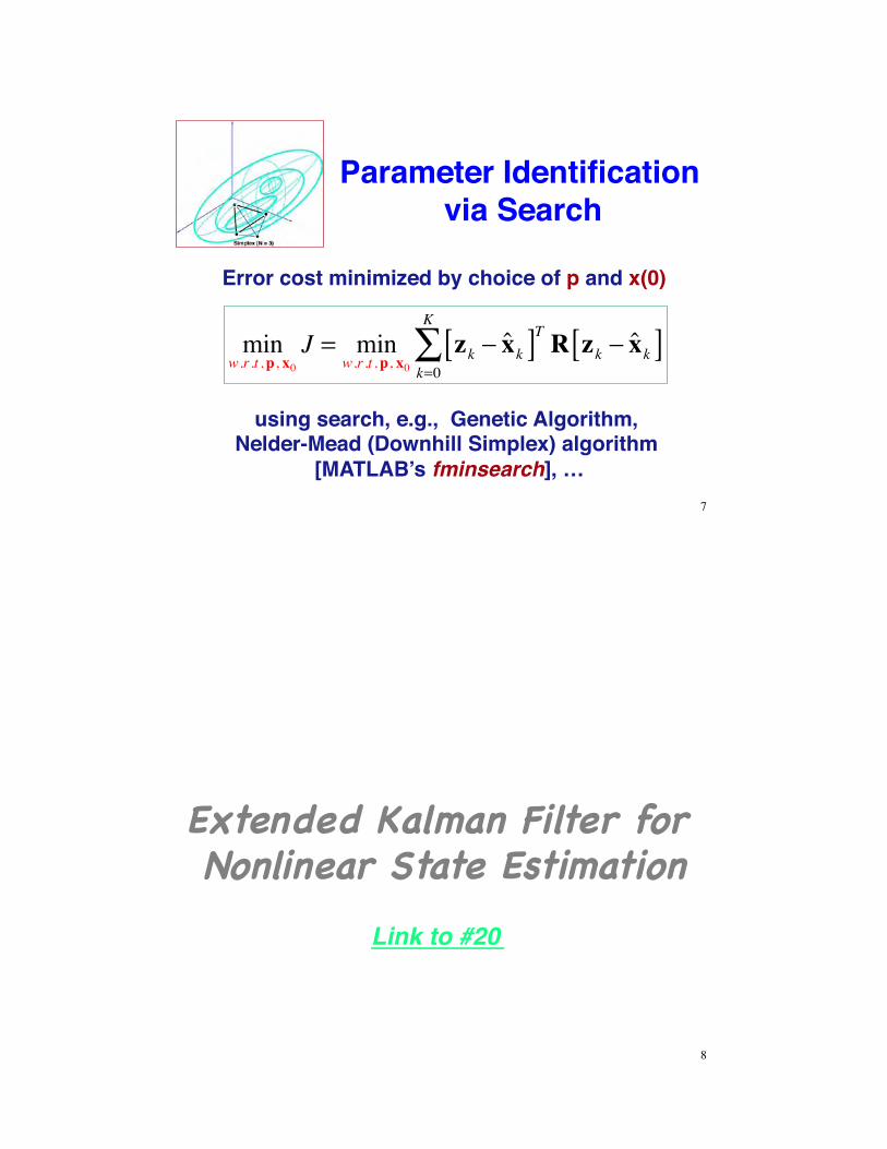
Parameter Identification via Search
Error cost minimized by choice of p and x(0)
minw.r .t .p, x0
J = minw.r .t .p, x0
zk ! x̂k[ ]T R zk ! x̂k[ ]k=0
K
"
using search, e.g., Genetic Algorithm, Nelder-Mead (Downhill Simplex) algorithm
[MATLAB’s fminsearch], …7
Extended Kalman Filter for Nonlinear State Estimation!
8
Link to #20

Extended Kalman-Bucy Filter
!! Propagate the state estimate using the continuous-time nonlinear model
!! Update the state estimate using an optimal continuous-time linear correction in the nonlinear propagation
!! Calculate optimal filter gain as in previous lecture and OCE
9
!̂x(t) = f x̂(t),u(t)[ ]+K t( ) z(t)! h x̂(t)[ ]{ }
Continuous-Time Nonlinear System
!x(t) = f x(t),u(t)[ ]z(t) = h x(t)[ ]+ n t( )
Hybrid Extended Kalman Filter
x̂k !( ) = x̂k!1 +( )+ f x̂ "( ),u "( )#$ %&d"tk!1
tk
'
Numerical integration for state and covariance propagation
Pk !( ) tk[ ] = Pk!1 +( )+ F "( )P "( ) + P "( )FT "( ) +L "( )Q 'C "( )LT "( )#$ %&d"tk!1
tk
'
State Estimate (–)
Covariance Estimate (–)
Jacobian matrices must be calculated
10

Hybrid Extended Kalman FilterIncorporate measurements at discrete
instants of time
Kk = Pk !( )HkT tk( ) HkPk !( )Hk
T +Rk!1"# $%!1
x̂k +( ) = x̂k !( ) +Kk zk !Hkx̂k !( )"# $%
Pk +( ) = In !KkHk[ ]Pk !( )
Filter Gain
Covariance Estimate (+)
State Estimate (+)
11
On-Line !(i.e., “real-time”)
Parameter Estimation!
12

Parameter Identification Using an Extended Kalman-Bucy Filter
!x(t)!p(t)
!
"##
$
%&&=
fx x(t),p(t),u(t),wx (t)[ ]fp p(t),wp (t)!" $%
!
"
##
$
%
&&; z = h x t( )!" $% + n t( )
Augment state to include the parameter
Extend the dynamic model to account for the parameter
13
Parameter Vector Must Have a Dynamic Model
Unknown constant parameter: p(t) = constant
!p t( ) = fp p t( ),wp (t)!" #$ " 0; p 0( ) = po; Pp 0( ) = PpoRandom parameter: p(t) = Integrated white noise
!p t( ) = fp p t( ),wp (t)!" #$ " wp t( ); p 0( ) = po; Pp 0( ) = PpoE wp t( )!" #$ = 0; E wp t( )wp
T %( )!" #$ =Qp& t '%( )
14
Several alternatives

!pM t( ) =!p t( )!pD t( )
!
"##
$
%&&= 0 I
0 0!
"#
$
%&
p t( )pD t( )
!
"##
$
%&&+
0wp t( )
!
"##
$
%&&
!pM t( ) =!p t( )!pD t( )!pA t( )
!
"
####
$
%
&&&&
=0 I 00 0 I0 0 0
!
"
###
$
%
&&&
p t( )pD t( )pA t( )
!
"
####
$
%
&&&&
+00
wp t( )
!
"
###
$
%
&&&
Dynamic Models for the Parameter Vector
Parameter vectorParameter rate of change
Parameter vectorParameter rate of changeParameter acceleration
15
Random parameter: p(t) = Integral of integrated white noise
Random parameter: p(t) = Double integral of integrated white noise
Number of parameters and derivatives to be estimated is doubled or tripled
Integrated White Noise Models of a Parameter
•! Third integral models slowly varying, smooth parameter
•! Second integral is smoother but still has fast changes
•! First integral of white noise has abrupt jumps, valleys, and peaks
•! White noise
16

Multiple-Model Testing for System Identification
Choose model with minimum error residual
17
Create a bank of Kalman Filters, one for each hypothetical model, n = 1,N
Jn = !! nk 'T R!! nk '
k '=k"ko
k
# = znk ' " x̂nk '$% &'TR znk ' " x̂nk '$% &'
k '=k"ko
k
#
Simultaneous Location and Mapping (SLAM)•! Build or update a local map within an
unknown environment–! Stochastic map, defined by mean and
covariance of many points–! SLAM Algorithm = State estimation with
bank of extended Kalman filters, a form of particle filter
–! Landmark and terrain tracking–! Multi-sensor integration
Durrant- Whyte et al
18

SLAM with Ultrasound SONAR, LIDAR, or RADAR
19UW-RSE Lab
Adaptive Control!
20

Reinforcement (“Q”) Learning•! Learn from success and failure•! Repetitive trials
–! Reward correct behavior–! Penalize incorrect behavior
•! Learn to control from a human operator
http://en.wikipedia.org/wiki/Reinforcement_learning21
Adaptive Control System Design•! Control logic changes to accommodate changes
or unknown parameters of the plant–! System identification to improve state estimate–!Gain scheduling to account for environmental change–!Adaptive Critic (Dual Heuristic Adaptive Dynamic
Programming)–! Learning systems that track performance metrics (e.g.,
CMAC)–!Reinforcement learning
•! Control law is nonlinear
u t( ) = c z(t),a,y * t( )!" #$
c •[ ] : Control lawx(t) : Statez x(t)[ ] : Measurement of statea : Control law parametersy*(t) : Command input
22
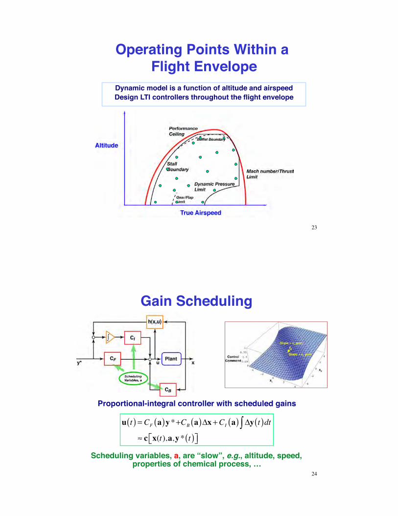
Operating Points Within a Flight Envelope
Dynamic model is a function of altitude and airspeedDesign LTI controllers throughout the flight envelope
23
Gain Scheduling
Proportional-integral controller with scheduled gains
u t( ) = CF a( )y*+CB a( )!x +CI a( ) !y t( )dt"# c x(t),a,y* t( )$% &'
Scheduling variables, a, are “slow”, e.g., altitude, speed, properties of chemical process, …
24

0200
400600
800
-1000
-500
0
6750
6800
6850
6900
6950
7000
7050With adaptation
Without adaptation
Adaptive Critic Neural Network Controller
•! On-line adaptive critic controller–!Replace gain matrices by neural networks (see Lecture 19)–!Nonlinear control law implemented as action network–! Performance and control usage evaluated via critic network–!Control network weights adapted to improve performance–!Cost model adapted to improve critique
25
Action Network On-line TrainingTrain action network, at time t, holding the critic parameters fixed
NNC
Aircraft Model •! Transition Matrices •! State Prediction
Utility Function Derivatives
NNA
xa(t)
a(t)
Optimality Condition
NNA Target
Target Generation 26

Critic Network On-line TrainingTrain critic network, at time t, holding the action parameters fixed
NNC(old)
Utility Function Derivatives
NNA
NNC Target
Target Generation
Aircraft Model •! Transition Matrices •! State Prediction
NNC
Target C ost Gradient
xa(t) a(t)
27
Real-Time Implementation of Rule-Based Control System
28

Application: Failure-tolerant flight control for CH-47 Chinook helicopter
Control is a side effect from expert system perspective
Rule-Based Control System (Handelman and Stengel, 1989)
29
•! Search until root node is solved–! Initiates lower-level
functions to declare leaf node is TRUE
Rule-Based Control Logic
30

Rule-Based Reconfiguration
Logic Example of a Failure-Diagnosis Rule
31
Failure ResponseResponse to Stuck Pitch-
Rate SensorResponse to Stuck Forward-
Collective Pitch Actuator
32

•! Original code written in LISP•! Automatic procedural code generation (LISP to Pascal)•! Real-time execution on three i386 processors in
Multibus™ architecture•! External PC used for code development, testing, and
helicopter simulation
Real-Time Implementation of Rule-Based Control System
33
Next Time:!Task Planning and Multi-
Agent Systems!
34

SSuupppplleemmeennttaarryy MMaatteerriiaall!!
35
Preferential Oxidizer (PrOx)
•! Proton-Exchange Membrane Fuel Cell converts hydrogen and oxygen to water and electrical power
•! Steam Reformer/Partial Oxidizer-Shift Reactor converts fuel (e.g., alcohol or gasoline) to H2, CO2, H2O, and CO. Fuel flow rate is proportional to power demand
•! CO poisons the fuel cell and must be removed from the reformate
•! Catalyst promotes oxidation of CO to CO2 over oxidation of H2 in a Preferential Oxidizer (PrOx)
•! PrOx reactions are nonlinear functions of catalyst, reformate composition, temperature, and air flow
FUELPROCESSOR
Shift
2H OAir
PrOx
Reformer or Partial Oxidation Reactor
36
Reinforcement ( Q ) Learning Control of a Markov Process
ubest tk( ) = argmaxu
Q x(tk ),u[ ]
•! Q: Quality of a state-action function•! Heuristic value function•! One-step philosophy for heuristic optimization
•! Various algorithms for computing best control value
Q-Learning Snailhttps://www.youtube.com/watch?v=UbwIPDaMlvY
Q-Learning, Ball on Platehttps://www.youtube.com/watch?v=04MLqlNZwHY&feature=related
Q x(tk+1),u(tk+1)[ ] =Q x(tk ),u(tk )[ ]+! (tk ) Lu(t ) x(tk )[ ]+ " (tk )maxuQ x(tk+1),u[ ]#
$%& 'Q x(tk ),u(tk )[ ]{ }
! (tk ) : learning rate, 0<! (tk )<1
37
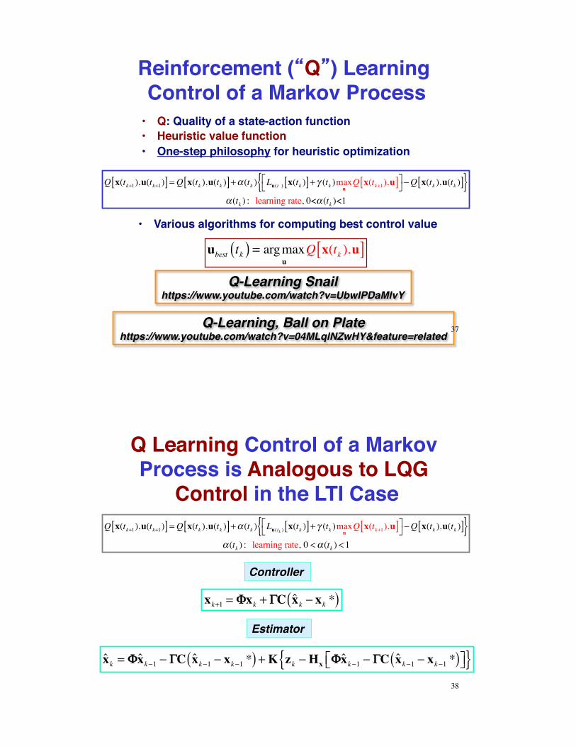
Q Learning Control of a Markov Process is Analogous to LQG
Control in the LTI CaseQ x(tk+1),u(tk+1)[ ] =Q x(tk ),u(tk )[ ]+! (tk ) Lu(tk ) x(tk )[ ]+ " (tk )max
uQ x(tk+1),u[ ]#
$%& 'Q x(tk ),u(tk )[ ]{ }
! (tk ) : learning rate, 0 <! (tk ) <1
xk+1 = !!xk + ""C x̂k # xk *( )
x̂k = !!x̂k"1 " ##C x̂k"1 " xk"1 *( ) +K zk "Hx !!x̂k"1 " ##C x̂k"1 " xk"1 *( )$% &'{ }
Controller
Estimator
38

More on Rules •! Example of a pre-formed compound rule
•! Once rule is defined, it has a fixed, ordered frame or argument list
•! Side effects: Actions triggered by inference–! If A = TRUE, … but what is A?–! Execute a function to find out, and return to the rule–! … then B = C, … but what is C?–! Execute a function …
39