task partitioning and scheduling on arbitrary parallel

AN ABSTRACT OF THE THESIS OF

Hesham El-Rewini for the degree of Doctor of Philosophy in Computer Science

presented on November 21. 1989.

Title: Task Partitioning and Scheduling on Arbitrary Parallel Processing Systems

Abstract approved:Redacted for Privacy

Theodore G. Lewis

Parallel programming is the major stumbling block preventing the parallel

processing industry from quickly satisfying the demand for parallel computer software.

This research is aimed at solving some of the problems of software development for

parallel computers.

ELGDF is a graphical language for designing parallel programs. The goal of

ELGDF is two-fold: 1) to provide a program design notation and computer-aided

software engineering tool, and 2) to provide a software description notation for use by

automated schedulers and performance analyzers. ELGDF is implemented as a graphical

editor called Parallax.

We extend previous results for optimally scheduling parallel program tasks on a

finite number of parallel processors. We introduce a new scheduling heuristic (MH) that

schedules program modules represented as nodes in a precedence task graph with

communication onto arbitrary machine topology taking contention into consideration.

We presents results for scheduling simulated task graphs on ring, star, mesh,

hypercube, and fully connected networks using MH.

We also present Task Grapher, a tool for studying optimal parallel program task

scheduling on arbitrarily interconnected parallel processors. Given a parallel program

represented as a precedence-constrained task graph, and an interconnect topology of a

target machine, Task Grapher produces the following displays: 1) Gantt Chart Schedule,

2) Speed-up Line Graph, 3) Critical Path In Task Graph, 4) Processor Utilization Chart,

5) Processor Efficiency Chart, 6) Dynamic Activity Display. Task Grapher currently

incorporates seven scheduling heuristics.

Finally, we introduce a new loop unrolling method for scheduling nested loops onto

arbitrary target machines. We use local neighborhood search and simulated annealing

methods to find: 1) the best unrolling vector, and 2) a Gantt chart that indicates the

allocation and the order of the tasks in the post-unrolled loop on the available processing

elements.

c Copyright by Hesham El-Rewini

November 21, 1989

All Rights Reserved

Task Partitioning and Scheduling on Arbitrary Parallel ProcessingSystems

by

Hesham El-Rewini

A THESIS

submitted to

Oregon State University

in partial fulfillment of

the requirements for the

degree of

Doctor of Philosophy

Completed November 21, 1989

Commencement June, 1990

APPROVED:

Redacted for PrivacyProfessor of Computer Science in Charge of Major

Redacted for PrivacyHead of Department of Computei\Science

Redacted for PrivacyDean of Graduate

Date thesis is presented November 21, 1989

Typed by Hesham El-Rewini for Hesham El-Rewini

Acknowledgements

I would like to express my appreciation to Dr. Ted Lewis for always displaying

confidence in my work and for the special effort he made as my major advisor.

I thank Dr. Walter Rudd for the many ways he lent his support both as committee

member and as department chairman. I thank Dr. Bella Bose for his friendship and for

those interesting discussions. I thank Dr. Bruce D'Ambrosio for his encouragement and

support. I thank Dr. David Sullivan for serving on my committee.

I thank the members of OACIS research team for the inspiring meetings and

discussions and for their constructive comments. In particular, I would like to thank

Inkyu Kim, Wan-Ju Su, Pat Fortner, and Juli Chu for helping me in translating my ideas

into running computer programs.

I want to thank each of the members of my family. I thank my mother for her

endless patience and encouragement. I thank my father for his support. I thank my

sisters for their love. And finally, A very special thank you to my brother Salah for his

encouragement and willingness to listen.

Table of Contents

1 Introduction 1

1.1 The Problem Statement 1

1.2 The Approach 3

1.2.1 Parallel Program Design 4

1.2.2 Parallel Program Scheduling 6

1.3 The Results 8

1.4 Outline of the Thesis 9

2 ELGDF: Design Language for Parallel Programming 11

2.1 Introduction 11

2.2 Overview of PPSE 12

2.3 Definition of ELGDF 15

2.3.1 Basic Constructs 16

2.3.2 Common Structures 21

2.3.3 Hierarchical Design 22

2.3.4 Mutual Exclusion 23

2.4 ELGDF Designs for Analysis 24

2.5 Example 25

2.6 Parallax Design Editor 29

2.7 Summary 33

Table of Contents continued

3 Static Mapping of Task Graphs with Communication onto

Arbitrary Target Machines 34

3.1 Introduction 34

3.2 List scheduling 36

3.3 Formulation of the Problem 37

3.3.1 Program Graph 37

3.3.2 Target Machine 37

3.3.3 System Parameters 38

3.4 The Mapping Heuristic (MH) 40

3.4.1 Definitions 41

3.4.2 MH 42

3.4.3 Complexity Analysis 50

3.4.4 Correctness of MH 51

3.5 Considering Contention in MH 52

3.5.1 MH Modifications 52

3.5.2 Adaptive Routing 55

3.5.2.1 Event_3 Update 59

3.5.2.2 Event 4 Update 63

3.5.3 How Good is MI-19 65


3.6 Simulation Results 75

3.6.1 Experiment 1 75



3.7 Task Grapher: A Tool for Scheduling Parallel Program Tasks 82

3.7.1 Task Grapher -- The Tool 82

3.7.2 Task Grapher Heuristics 88

3.7.3 Output From Task Grapher 92

3.8 Summary 97

4 Loop Unrolling 99

4.1 Introduction 99

4.2 Dependence Among Tasks 101

4.2.1 Dependence Between Tasks within loops 101

4.2.2 Dependency Matrix (DM) 103

4.3 Loop Unrolling 105

4.4 Execution Time in Nested Loops 113

4.4.1 Definitions 113

4.4.2 Execution Time Formulas 114

4.5 Combinatorial Minimization 117


4.6 Loop Unrolling Problem Formulation 119

4.7 Examples 121

4.7.1 Case 1: Single Loop (n = 1) 121

4.7.2 Case 2: Two Nested Loops (n = 2) 127

4.7.3 Case 3: Three Nested Loops (n = 3) 130

4.8 Summary 133

5 Conclusions and Future Work 135

5.1 Conclusions 135

5.2 Future Work 137

5.3 Thoughts about Scheduling Task Graphs with Branches 138

5.3.1 Probabilistic Program Model 139

5.3.2 Deterministic Task Graphs 140

5.3.2.1 Expected Task Graph 140

5.3.2.2 Most Likely Task Graph 141

5.3.2.3 Random Task Graph 141

5.3.3 Example 142

Bibliography 145

List of Figures

Figure

2.1 Overview of PPSE 14

2.2 An ELGDF Design Network 15

2.3 An ELGDF Subnetwork With Node P(i) Replicated N Times and its

Expansion When N = 3 18

2.4 A Pipe X(N,m) of Node P(i) and its Expansion 19

2.5 A For Loop Construct and its Unrolling 3 Times 20

2.6 A Fan of Size n and its Expansion 21

2.7 Hierarchical Design 22

2.8 Mutual Exclusion 23

2.9 System of Equations AX = B 27

2.10 Top Down Solution for AX = B 28

2.11 Parallax Design Palette 30

2.12 Packing 4 Nodes and 4 Arcs. 31

2.13 A Packed Design Network 31

2.14 A Subnetwork in a Separate Window Using Go-Down 32

2.15 Connecting Two Nodes in Two Different Windows Using Bridge 32

3.1 Example of Task Graph. 40

3.2 Example of Target Machine 40

List of Figures continued

3.3 Gantt Chart Resulting From Scheduling Task Graph (TG1) on Target

Machine (TM1). 41

3.4a The MH Algorithm 44

3.4b Initialize Event List Routine 44

3.4c Process Event Routine 45

3.4d Schedule Task Routine. 45

3.4e Handle Successors Routine 46

3.4f Insert Event Routine. 47

3.4g Locate Processor Routine. 48

3.4h Finish Time Function. 48

3.5 (a) Task Graph, (b) Hypercube Target Machine, and (c) the Resulting

Gantt Chart 49

3.6 (a) Target Machine With 4 Processing Elements, and (b) the Initial Tables

Associated With Each Processing Element 54

3.7 Process Event Routine (with contention) 57

3.8 Schedule Task Routine (with contention). 58

3.9a Direct_Effect_on_the_Route_Event_3 59

3.9b Update_Delay Routines 60

3.9c Tables 0 and 1 After the Direct Effect Update 60

3.10a Indirect_Effect_on_Neighbors 61


3.10b Update_Neighbors Routines

3.10c Input From 0, 3 and the New Table for 2.

62

63

3.11 Direct_Effect_on_the_Route_Event 4 Routine 63

3.12 (a) Task Graph, (b) Target Machine, (c) MH Schedule, and (d) Optimal

Schedule 68

3.13 (a) Task Graph, (b) Target Machine, and (c) MH Schedule (Optimal) 69

3.14 (a) Task Graph, (b) Target Machine, and (c) MH Schedule (Optimal). 70


Schedule 71


Schedule 72


Schedule 73

3.18 (a) MH Schedule and (b) Optimal Schedule for scheduling the Task Graph

used in Figure 3.17 after increasing the size of task 5. 74

3.19 Speed_Up Curves for 5 Different Target Machines 76

3.20 Using Communication in Calculating the Level in MH 77

3.21 When Using Communication in Calculating the Level is Better. 78

3.22 When Using Communication in Calculating the Level is Worse. 78

3.23 The Effect of Changing the Communication-Execution Ratio on the

Speed_Up Curves when Using Different Hypercubes as Target Machine. 80


3.24 The Effect of Changing Task Graph Average Degree on the Speed Up

Curves when Using Different Hypercubes as Target Machine. 81

3.25 A Task Graph Consists of Nodes and Arcs. The Integer in the Upper

Portion of Each Node is the Node Number. The Integer in the Lower

Portion is an Execution Time Estimate. The Arcs are Labeled with a

Communication Message Size Estimate. 83

3.26 Gantt Chart Produced by Task Grapher. Processor Numbers are Shown

Across the Top, and Time is Shown Down the Left Side. Light Shaded

Regions Show a Task Waiting for Communication, and Dark Shaded

Regions Show When Tasks Execute 84

3.27 Speed-Up Line Graph of the Task Graph Given in Figure 3.18 for a Fully

Connected Parallel Processor System. Six Scheduling Algorithms Yield

Three Different Schedules 86

3.28 Fully Connected Interprocessor Connection Topology. Any Connection

Topology can be Evaluated by Entering the Topology into this Screen 87

3.29 Critical Path in the Task Graph of Figure 3.18 The Shaded Nodes Show

Which Nodes Lie Along the Path of the Greatest Execution Time. 88

3.30 The Basic Scheduling Algorithm 89

3.31 Processor Utilization Chart of a Target Machine With Six Processors.

Produced by Task Grapher 94

3.32 Average Processor Efficiency Chart Produced by Task Grapher 95

3.33 Dynamic Activity Display of a Task Graph on 6 Processors Forming a

Fully Connected Machine. At the Time of the Snap Shot Tasks 1, 2, 7,

10, 15, and 46 were Assigned to Processors 2, 0, 5, 3, 4, and 1

Respectively 96


4.1 Three Tasks in Single Loop 103

4.2 DM and TSA for Two Tasks a and b Enclosed in Two Nested Loops. 106

4.3 An Example for Unrolling a Single Loop Once (u = <1>). 106

4.4 (a) Original Loop, (b) Innermost Loop is Unrolled Once (u = <0,1>), (c)

Outermost Loop is Unrolled Once (u = <1,0>), and (d) Both Loops are

Unrolled once each (u = <1,1>) 107

4.5 DM and TSA for Two Tasks a and b Enclosed in a Single Loop 109

4.6 Gantt Charts Result From Scheduling Four Iterations of the Loop on One

and Two Processing Elements 110

4.7 Gantt Chart Results From Scheduling Two Iterations of the Unrolled

Loop on Two Processing Elements 110

4.8 Two Tasks a and b Enclosed in Two Nested Loops Represented Using

DM and TSA 111

4.9 (a) Original Loop, (b) the Loop After Unrolling the Outermost Loop Once,

and (c) the Loop After Unrolling the Innermost Loop Once. 112

4.10 (a) The Schedule After Unrolling the Outermost Loop Once, and (b) the

Schedule After Unrolling the Innermost Loop Once. 112

4.11 Gu That Represents Lu, Represented by DM and TSA Given in Figure

4.2, when u = <1,1 >. 114

4.12 Objective Function Evaluation 120

4.13 DM and TSA for Four Tasks (1, 2, 3,and 4) Enclosed in a Single Loop. 123

4.14 The Change in E when the Loop is Unrolled From 4 to 21 Exhaustively

(n=1) 124


4.15 Three Successful Moves in Local Neighborhood Search (n=1) 125

4.16 Nine Successful Moves in Simulated Annealing (n = 1) 126

4.17 DM and TSA for Three Tasks (1, 2,and 3) Enclosed in Two Nested

Loops. 127

4.18 Five Successful Moves in Local Neighborhood Search (n = 2) 128

4.19 Eleven Successful Moves in Simulated Annealing (n = 2) 129

4.20 DM and TSA for Three Tasks (1, 2, and 3) Enclosed in Three Nested

Loops. 130

4.21 Six Successful Moves in Local Neighborhood Search (n = 3) 131

4.22 Nine Successful Moves in Simulated Annealing (n = 3). 132

5.1 Data Dependency Graph (DDG) 143

5.2 Branch Activation Graph (BAG) 143

5.3 Expected Task Graph (ETG) 144

5.4 Most Likely Task Graph (MTG) 144

5.5 Random Task Graph (RTG) 144a

List of Tables

Table

4.1 Exhaustive Search (n = 1) 124

4.2 Local Neighborhood Search (n = 1) 125

4.3 Simulated Annealing Solution (n = 1) 126





Task Partitioning and Scheduling on Arbitrary Parallel ProcessingSystems

Chapter 1

Introduction

1.1 The Problem Statement

Since humans tend to think sequentially rather than concurrently, program

development is most naturally done in a sequential language [A1Ke85]. Unfortunately

sequential programming is incapable of directly making effective use of parallel

computers.

A wide variety of parallel computer architectures are commercially available. These

range from shared-memory multiprocessors to reconfigurable networks of distributed-

memory multiprocessors. Parallel computing hardware will continue to evolve along

many architectural lines, and research will continue to improve the performance and lower

the cost of this hardware. But the lack of good software development tools and

techniques for programming parallel computers is the most significant problem facing

parallel computing. Accordingly, the research described in this thesis is aimed at solving

some of the problems of software development for parallel computers.

One significant problem that parallel programming faces is portability and

compatibility. As new parallel computer architectures appear, the diversity of parallel

programming systems increases. Different manufacturers introduce different parallel

programming primitives added to sequential languages or entirely new parallel languages

which make parallel programming quite architecture-dependent. Developing hand-coded

2

parallel programs is equivalent, in a sense, to programming in a low level

sequential language, because hand-coded parallel programs are architecture dependent.

For example synchronization is done using locks in a shared memory architecture, but

synchronization is done via message passing in a distributed memory architecture.

A second major problem is concerned with how to schedule the parallel tasks

forming a program onto a particular parallel computer so the program completes at the

shortest time. In order to efficiently use parallel computers, programmers have to find the

best mapping of the program tasks onto the available processors. Theoretically, this

problem is mathematically complex and often requires exponential time to solve for the

absolute best schedule [Car184, CoGr72, Ullm75].

Software development is intrinsically difficult and time consuming for both

sequential and parallel computing applications. However, designing and writing software

for parallel computers is even more difficult because programmers have a great many

details to worry about at any time. A parallel programmer must keep details of non-

determinism, race conditions, synchronization, and scheduling.

It is not surprising that an architecture-independent higher abstraction is needed so

program designers can express their algorithms in high level structures without having to

worry about details such as synchronization.

More realistic scheduling heuristic algorithms that consider the important features

needed to model modern parallel processor systems (inter-processor connection and

contention for example) are also needed so high level parallel programs can be analyzed

and translated into schedulable units of computation that fit the target hardware

architecture.

3

In order to ease parallel program development, software tools for designing and

tuning parallel programs are needed to optimize the performance on a given target

machine.

1.2 The Approach

There are two principal approaches being taken by parallel programming

researchers: 1) implicit, and 2) explicit parallelism [Lewi89].

In the implicit approach, existing and new languages are used to conceal the

underlying parallel computer from the programmer. Intelligent high-level compilers must

be designed to automatically translate the high-level application into parallel form.

In the explicit approach, the programmer must know about parallelism, and the

programming language must incorporate explicit parallel control statements in its syntax.

Explicit parallel programmers need sophisticated tools to assist in writing correct and fast

parallel software.

Clearly, the implicit approach is highly desirable because it removes the burden

from the shoulders of programmers. But, the burden is shifted to the compiler writer.

Designing such a compiler appears to be an exceptionally difficult problem.

The implicit approach requires "genius" compiler. The explicit approach requires

"clever" programmer. We think that it is easier to develop tools and techniques that help

the programmer to be "clever" than to develop a "genius" compiler. Consequently, we

decided to take the explicit approach.

In this research, we focus in two problems in the explicit approach: 1) parallel

program design (how to partition an application into parallel parts using an architecture-

4

independent design language), and 2) parallel program scheduling (how to optimally

schedule and run parallel tasks onto a given target machine).

1.2.1 Parallel Program Design

Sequential programming evolved from architecture-specific low level languages.

Then high level architecture-independent languages appeared so programmers did not

have to worry about architectural details. Finally, extensions have been made to high

level languages to make them more structured and abstract leading to programs that are

easier to develop, test, and maintain. We believe that parallel programming should evolve

in the same direction.

Two major problems face parallel program designers: 1) In a given program, how

does one identify regions of code that can be executed in parallel with minimum

synchronization? , and 2) once a program has been partitioned for parallel execution, how

does one keep memory access conflicts and synchronization delays from degrading

performance to an unacceptable level? These problems can be solved by a clever

programmer, but they require intimate knowledge of both the program and the machine

hardware. Parallel programming is so tedious that some form of automatic or semi-

automatic assistance is very desirable. But what form should that assistance take? We

believe that an architecture-independent higher abstraction that captures program design

features is needed so a programmer can start with an initial design description, and

iteratively use scheduling and performance estimating tools to arrive at a better design on

a given architecture.

Three goals to be achieved in a good design language are: 1) Programming for

portability, 2) generating efficient target code in high-level language (C, FORTRAN), and

3) easing the cost of programming.

5

Currently research is centered around providing high level architecture-independent

models for representing parallel programs. Large grain dataflow networks [Babb84,

BaDi87, DiBa88, DiNu89a, DiNu89b] have been used to express parallel programs.

Browne, Azam, and Sobek [BASo89] have introduced an architecture-independent

language, called CODE, for visually, describing parallel programs as computation units,

dependency relations among them, and firing rules. It raises the abstraction level at

which one specifies dependencies and firing rules to permit downward translation to

many architectures. Booster [PaSi89] is another high level language that is especially

suited to program problems which have array-like structures as their underlying data

structure. Petri nets have also been used as a model for parallel program description as in

[AdBr86, Stott88]. Davis and Keller [DaKe82] think that graphs can be used to present

an intuitive view of the potential concurrency in the execution of the program. A survey

of current graphical programming techniques can be found in [Raed85]. Snyder has

introduced a graphical programming environment called Poker [Snyd84] that supplies a

mechanism to draw a picture of a graph representing the communication structure among

sequential processes. It also furnishes data driven semantics with coordination for

synchronization to run the program. Kimura [Kimu88] has also presented a visual

programming approach for describing transaction-based systems. A tool for developing

and analyzing parallel FORTRAN programs called SCHEDULE is given in [DoSo87].

SCHEDULE requires a user to specify the subroutine calls along with the execution

dependencies in order to carry out a parallel computation.

We believe that an efficient parallel program design can be achieved through

iterative interaction between the user and the parallel programming system. An

architecture-independent notation is needed to capture parallel program design features for

analysis purposes. A set of software tools is needed to help in the tuning process required

by parallel programs to optimize performance.

6

Since dataflow [Acke82, DaKe82, Denn80] has the advantage of allowing program

definitions to be represented exclusively by graphs, in this research we introduce an

architecture-independent graphical design notation for parallel programming called

ELGDF (Extended Large Grain Dataflow). ELGDF is part of the Parallel Programming

Support Environment (PPSE) [Lewi89]. The goal of ELGDF is to ease describing

parallel programs and to provide the PPSE tools with the needed information about the

design at hand.

1.2.2 Parallel Program Scheduling

The problem of optimally scheduling n tasks onto m processors has been studied

for many years by many researchers. An optimal schedule is an allocation and ordering

of n tasks on 13.m processors such that the n tasks complete in the shortest time. We

distinguish between allocation and scheduling (allocation and ordering): an allocation is

an assignment of the n tasks to m or fewer processors [Bokh81 a, Bokh81 b, ChSh86,

CHLE80, Lo84, RELM87]. An allocation may result in a non-optimal schedule, because

the order of execution of each task as well as which processor it is assigned to determines

the time to completion of successor tasks in the parallel program.

Tasks can be scheduled on parallel processors using two fundamentally different

approaches: 1) dynamic, and 2) static. In the dynamic approach, scheduling is done on

the fly -- as the program executes. This approach is useful when the parallel program has

loops and branches whose execution time cannot be determined beforehand. For

example, the number of iterations of a loop may not be known until the program

executes, or the direction of a branch may be unknown until the program is midway in

execution [DLRi82, Tows86j. It is difficult to achieve optimal or even near-optimal

schedules for single parallel programs with this method. However, dynamic scheduling

can be used in time-shared systems to achieve load balancing [ChAb811.

7

In static scheduling, one attempts to determine the best schedule prior to program

execution by considering task execution times, communication delays, processor

interconnections, and other factors [Car184, GGJo78, Gonz77]. The results reported

here apply to static scheduling, and may not be applicable to dynamic scheduling.

The earliest result for static scheduling seems to have been reported by Hu in 1961

[Hu61]. A restricted two-processor solution was later given by Coffman [CoGr72].

But, Hu's and Coffman's algorithms solved an abstract version of the problem which

ignored most of the critically important features needed to model modern parallel

processor systems: 1) tasks may have different execution times, 2) communication links

between tasks may consume a variable amount of communication time, 3) communication

links may be themselves shared, thus giving rise to contention for the links, 4) the

network topology may influence the schedule due to multiple-hop links, or missing links,

and 5) the parallel program may contain loops and branches, hence the task graph may

become complex and unmanageable.

A more recent survey by Casavant [CaKu88] and related studies [Car184, CoGr72,

Ullm75] have shown that optimal task scheduling is a computationally intense problem.

The complexity of the problem rises even further when real-world factors such as

interconnection topology and link contention are considered.

To reduce the complexity of the problem, most investigators make two simplifying

assumptions: 1) the parallel program can be represented by a precedence-constrained task

graph, and 2) sub-optimal solutions achieved by fast heuristic algorithms are suitable for

practical application. In a precedence-constrained task graph, each node represents a

process or task and arcs represent inputs from one or more predecessor tasks. Tasks

execute to completion and then send one or more messages to one or more successor

tasks.

8

Adam, Chandy, and Dickson [ACDi74] showed that the class of "highest-level-

first" (HLF) heuristics are best for estimating a static schedule. Following their advice,

the HLF approach has been used and modified by a number of researchers to overcome

limitations. Most of the effort has explained the addition of communication delays

between processors [Krua87, LHCA88, Linn85, Pars87, YuHo84].

Currently, research is centered around finding heuristics which work on task graphs

with communication and trade task duplication for communication delay [Krua87]. These

algorithms are described elsewhere, and a discussion of the complexity of this approach

can be found in [Car184].

Our research in this area is focused in two directions: 1) scheduling parallel program

tasks represented as task graphs with communication onto arbitrary processor

interconnection topology taking contention into consideration, and 2) scheduling nested

loops with unknown bounds onto arbitrary processor interconnection topologies through

loop unrolling.

1.3 The Results

In this research we introduce: 1) ELGDF: a high level graphical design language for

parallel program design, 2) MH: a new scheduling heuristic that considers the topology of

the target machine and contention, 3) simulation results for scheduling simulated task

graphs on ring, star, mesh, hypercube, and fully connected networks, 4) a new loop

unrolling technique for scheduling nested loops onto arbitrary target machines, and 5)

Parallax Design Editor and Task Grapher: tools for designing and scheduling parallel

programs, respectively.

ELGDF extends LGDF and LGDF2 [Babb84, BaDi87, DiBa88, DiNu89a,

DiNu89b] as follows: 1) high level structures are provided such as replicators, loops,

9

pipes, etc. to ease programming and increase "expressiveness", 2) branch and loop

constructs are provided which give more information for scheduling and analysis

purposes, 3) parameterized constructs are provided so that compact graphical

representations of design are possible, 4) arc overloading is resolved by providing

different symbols and different attributes for different types of arcs to remove confusion

and increase program readability, 5) mutual exclusion for shared memory systems can be

easily expressed, 6) synchronized pipelining is provided through repeated arcs, and 7)

ELGDF captures program design features so they can be stored for use by analysis tools.

The mapping heuristic (MH) schedules program modules represented as nodes in a

precedence task graph with communication onto machine with arbitrary topologies. MH

gives an allocation and ordering of tasks onto processors. Contention is considered in

MH so more realistic schedules and timing information can be produced. MH also keeps

contention information in tables and updates them when certain events take place so it can

make scheduling decisions based on a current traffic state. The significance of this work

is that we can now begin to schedule task graphs onto multiprocessor systems in an

optimal way by considering the target machine, communication delays, contention, and

the balance between computation and communication.

The loop unrolling method allows several iterations of a set of loops as well as

tasks within the same iteration to overlap in execution in such a way that minimizes the

iteration initiation interval and the loop execution time. We use local neighborhood search

and simulated annealing techniques to achieve near optimal execution times.

1.4 Outline of the Thesis

This thesis is organized into five chapters as follows. In chapter 2 we first

introduce the ELGDF design language, then we present the Parallax design editor as a

tool for expressing parallel program designs in ELGDF. The MH scheduling heuristic

10

for scheduling task graphs onto arbitrary target machines is discussed in chapter 3.

Chapter 3 also contains some simulation results and presents the Task Grapher tool for

scheduling parallel program tasks. Chapter 4 introduces a new loop unrolling method

that is used to schedule nested loops onto arbitrary target machines using local

neighborhood search and simulated annealing optimization techniques. Finally, Chapter

5 contains conclusions and recommendations for future work.

11

Chapter 2

ELGDF: Design Language for Parallel Programming

2.1 Introduction

ELGDF (Extended Large Grain Data Flow) is a graphical language for designing

parallel programs. The goal of ELGDF is two-fold: 1) to provide a program design

notation and computer-aided software engineering tool, and 2) to provide a software

description notation for use by automated schedulers and performance analyzers. The

syntax is hierarchical to allow construction and viewing of realistically sized applications.

ELGDF is a program design language, and not a programming language, but an ELGDF

design can be transformed into Pascal, C, FORTRAN, etc. source code programs

through.

ELGDF facilitates describing parallel programs in a natural way for both shared-

memory and message-passing models using architecture-independent higher abstractions

that allow program designers to express their algorithms in high level structures such as

replicators, loops, pipes, branches, and fans. The arc overloading that occurs in other

graphical languages [Babb84, BaDi87, DiBa88, DiNu89a, DiNu89b] is resolved in

ELGDF by using different symbols and different attributes for different types of arcs.

ELGDF notations are used in the PPSE (Parallel Programming Support

Environment) [Lewi89] for expressing parallel designs. Parallax is a graphical design

editor implemented for that purpose [Kim89]. Using Parallax, the parallel design features

and code fragments are stored in files called the PP design files for use by other tools in

the PPSE such as Task Grapher, SuperGlue, and EPA [RLEJ89]. For example task

graphs at different levels of granularity can be extracted from the PP design files for use

12

by scheduling tools. Estimated execution time of tasks at different levels of granularity

can also be used by performance evaluation tools.

We believe that using ELGDF design language will ease software development for

parallel computers, will help programmer comprehension and will help produce parallel

program designs in a form appropriate for analysis.

The rest of this chapter is organized as follows. We give a brief overview of PPSE

in section 2.2. The definition of the proposed design language is given in section 2.3.

Section 2.4 shows ELGDF designs for analysis and an example is given in section 2.5.

The Parallax design editor is described in section 2.6. Finally we give our summary in

section 2.7.

2.2 Overview of PPSE

The Parallel Programming Support Environment (PPSE) is a set of software tools

designed to help parallel programmers deal with forward and reverse engineering of

parallel software. Forward engineering deals with the task of writing new parallel

programs. Reverse engineering involves retrofitting existing sequential programs onto

parallel computers. The interaction among different tools in PPSE are shown in Figure

2.1.

From the forward engineering perspective a parallel program designer uses the

Parallax Design Editor to construct an ELGDF design for the desired program. The

dataflow graph, which describes the interconnections and data dependencies, and other

design features of the proposed program are stored in the PP design file. In addition,

code fragments are stored for later use when the time comes to generate the application's

source code.

13

Similarly, the target machine(s) is described using the Target Machine Editor

[RLEJ89] and its description is stored in the topology files. The topology file contains

the architectural properties of the target machine, such as interconnection topology,

transmission speeds, and cache structure.

The programmer next uses the Task Grapher tool to allocate and schedule the

parallel tasks onto the given target machine(s). The Task Grapher produces the schedule

in the form of a Gantt chart of processing elements versus time. The output of the Task

Grapher also includes speed-up curves (showing the anticipated speed-up versus number

of processing elements) and other performance displays such as utilization and efficiency.

The Super Glue tool [Hand89] uses the code fragments, library routines, and the

Gantt chart to produce parallel source code to run on a given architecture. The library

routines are needed to tailor each application to a specific target machine.

When the resulting program is actually compiled and run on the target machine,

additional statistics are collected and used by the performance analysis tools to generate an

actual Gantt chart and performance reports. Having the actual Gantt chart and the

performance feedback, the user may want to tune the design to improve the performance.

Similarly, we are developing a system in which an existing serial program can be

reverse engineered by re-casting it as an ELGDF design [HaGi89]. In this scenario, a

serial source code program would be read into the PPSE and dependency information

extracted to construct an ELGDF network of the program. Once we have the ELGDF

network of the serial program, all the forward engineering tools can be used to restructure

the program into parallel version.

The reverse engineering tool [HaGi89] also translates a serial program into a

database so that questions in the form of database queries can be asked about the

14

program. For example queries about the data dependency between program parts can be

asked so the programmer can then restructure the program to remove the dependency to

increase parallelism.

ELGDF DesignSpecification

iParallax Design

Editor,

.1...Fragments

Dusty Deck

1Reverse

Engineering

PP Design

eTask Graph Task GraphsGenerator

Library

Super Glue)

Gantt Chart

II! Compile

So

_piLinkurce Code Run

eTarget Machine

Editor

Topology

Mapping Display

Actual Chart1Performance

AnalysiszProfile Stats

Figure 2.1 Overview of PPSE

15

2.3 Definition of ELGDF

ELGDF is rich enough to express the common control structures found in parallel

programs [ElLe89a]. An ELGDF design takes the form of a directed network consisting

of nodes, storage constructs, parameterized constructs, control structures, and arcs.

Figure 2.2 shows an ELGDF design network at some level in the hierarchy.

Figure 2.2 An ELGDF Design Network

16

2.3.1 Basic Constructs

Nodes

A node, as shown in Figure 2.2, is represented by a "bubble," and can represent

either a simple or a compound node. A simple node consists of sequentially executed

code and is carried out by at most one processor. A compound node is a decomposable

high level abstraction of a subnetwork of the program design network.

Storage Constructs

A storage construct is represented by a rectangle, and can represent either a storage

cell or a collection of storage cells. A storage cell represents the data item to be read or

written by a simple node.

A node connected to the top of a storage construct has access to it before any node

connected to its bottom. Nodes connected to a storage construct on the same side

(top/bottom) compete to gain access to that storage construct in any order. A shared

storage cell X is used in Figure 2.2.

A compound node connected to the left or the right sides of a rectangle representing

a collection of storage cells means that the compound node accesses the constituents of

the storage collection, but the details are given in a lower level description.

Arcs

An arc in ELGDF can express either data dependency, sequencing, transfer of

control, or read and/or write access to a storage construct. A set of attributes is associated

with each arc to provide information about the arc type, data to be passed through the arc,

storage access policy, and communication strategy. An arc can be either a simple arc

17

which cannot be decomposed or a compound arc which is decomposable into a set of

other simple and/or compound arcs.

Simple arcs can be classified into control and data arcs. A control arc, as shown in

Figure 2.2 (dotted line) expresses sequencing or transfer of control among nodes. A data

arc carries data from one node to another or can connect a node to a storage construct. A

data arc connecting a node and a storage construct can represent READ, WRITE, or

READ/WRITE access according to the direction of the arc.

A data arc can be used to carry data once or repeated times per activation. One of

the arc's attributes is used to indicate the number of times data will be passed through it.

If the value of that attribute is greater than one then the arc is considered a repeated arc.

The repeated arc is used basically in pipelines. It can carry data from a simple node to

another in a synchronized fashion. Also it can express synchronized writing and reading

to or from a storage cell.

Split and Merge

Split and merge, as in Figure 2.2, are special purpose simple nodes for representing

conditional branching. Split has two output control-arcs; one for T = True, and the other

for F = False. According to the truth or the falsehood of the condition associated with the

split node one of its two output control arcs is activated. Merge has N input control arcs

and one output control arc. Merge activates its output arc when it gets activated by any

one of its N inputs.

18

Replicators

A replicator, as used in Figure 2.2, is one of the parameterized constructs in

ELGDF that allows program designers to represent concurrent loop iterations compactly.

A set of attributes is associated with the replicator such as the control variable, initial

value, step, and replicator bound. Replication of a node N times produces N concurrent

instances of that node. An arc connected to a replicator is expanded as a set of identical

arcs each of which is connected to one of the replicated instances. Figure 2.3 shows an

ELGDF subnetwork that contains a replicator over a node P(i) (i = 1 to N), and its

expansion when N = 3.

simple node

N = 3replicator

simple node

Figure 2.3 An ELGDF Subnetwork With Node P(i) Replicated N Times and its

Expansion When N = 3.

19

Pipes

A pipe, as in Figure 2.4, is a high level abstraction that allows program designers

to compactly represent a set of N nodes forming a pipeline . The pipe consists of N

simple nodes and N-1 m-repeated arcs. The nodes forming the pipeline are replications

of the same simple node. A pipe has several attributes associated with it such as number

of stages in the pipeline (N), number of times the data will be passed through repeated

arcs in the pipe (m) and others [E1Le89]. Figure 2.4 shows a pipe X(N,m) of node P(i)

and its expansion.

Loops

stages = N

number oftimes dataare passed = m

C=>

X

pipe: X(N,m) of node P(i)

m-repeated arc

m-repeated arc

m-repeated arc

Figure 2.4 A Pipe X(N,m) of Node P(i) and its Expansion.

A loop can represent For, While, or Repeat structures. ELGDF allows program

designers to express loops compactly by using single icons to represent cycles. This is

20

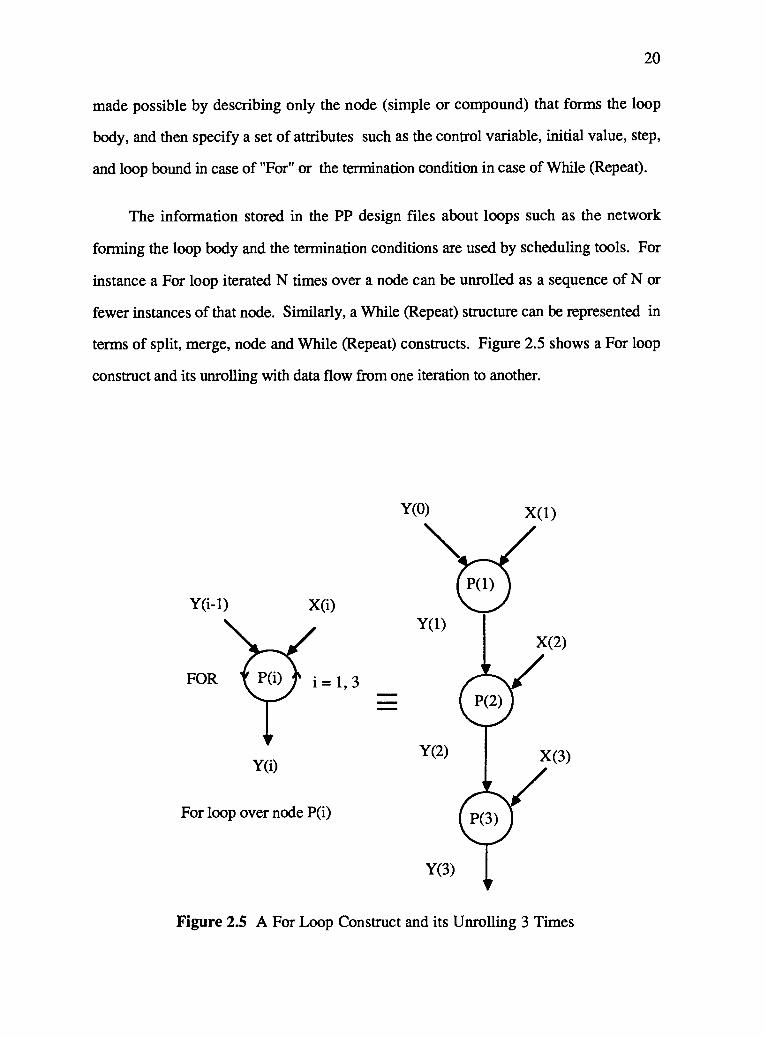
made possible by describing only the node (simple or compound) that forms the loop

body, and then specify a set of attributes such as the control variable, initial value, step,

and loop bound in case of "For" or the termination condition in case of While (Repeat).

The information stored in the PP design files about loops such as the network

forming the loop body and the termination conditions are used by scheduling tools. For

instance a For loop iterated N times over a node can be unrolled as a sequence of N or

fewer instances of that node. Similarly, a While (Repeat) structure can be represented in

terms of split, merge, node and While (Repeat) constructs. Figure 2.5 shows a For loop

construct and its unrolling with data flow from one iteration to another.

Y(i-1)

FOR

X(i)

Y(i)

For loop over node P(i)

Y(0) X(1)

Figure 2.5 A For Loop Construct and its Unrolling 3 Times

21

2.3.2 Common Structures

ELGDF also supports many of the common structures in parallel programs that can

be synthesized using the constructs given above [ElLe89a]. It automatically provides

them for program designer convenience. Complete trees, meshes, branches, and fans are

examples of common structures. The system can prepare skeletons for various types of

structures per designer request. Using these structures reduces the drawing time, helps

design readability and comprehension, gives more information for analysis tools

(regularity of trees for instance).

For example, a fan of size n is composed of a start node S, n parallel nodes Pi, i =

[1..n], 2n control arcs aj, j = [1..2n], and an end node (E). Figure 2.6 shows a fan of

size n and its expansion. Arc aj connects S to Pj, j = [1..n]. Arc ak connects Pk_n to E, k

= [n+1..2n]. The start node activates the parallel nodes and when they all finish E gets

activated. Compound arcs that are connected to a fan carry data to or from its

constituents.

Fan of size n

Figure 2.6 A Fan of Size n and its Expansion

22

2.3.3 Hierarchical Design

ELGDF supports hierarchical design to allow construction and viewing of

realistically sized applications. Figure 2.7 shows a hierarchical network, a compound

arc going from compound node A to compound node B having X, Y as data structure

associated with it. Thus, some constituents in B are data dependent on some

constituents in A and the data involved are X, Y. In the lower level decomposition of A

and B , node b0 needs X from node a0 and node bl needs Y from node a2.

top level design

A decompositionB decomposition

Figure 2.7 Hierarchical Design

23

2.3.4 Mutual Exclusion

ELGDF helps designers to easily express mutually exclusive access to shared

variables by having an exclusion attribute associated with each data arc connecting a node

to a storage construct. If the exclusion attribute is set, then mutual exclusion access for

the data structure associated by the storage construct is requested.

Figure 2.8 shows three simple nodes A, B, and C and a storage cell X forming an

ELGDF network. Nodes A, B, and C share the variable X, yet A and B have access to X

before C because A and B are connected to the top of X and C is connected to the bottom.

A and B can access X in any order since they are both in the top side of X. Both A and B

want to update X through a READ/WRITE arc and that might produce an incorrect result

unless we set the mutual exclusion attribute (exclusion) associated with those

READ/WRITE arcs to guarantee mutual exclusive access to X as shown.

READ/WRITEdata arcs

exclusion: ON exclusion: ON

READ data arc

Figure 2.8 Mutual Exclusion

24

2.4 ELGDF Designs for Analysis

ELGDF provides the information needed by different analysis tools in the PPSE, so

that program designers can get feedback and try different forms of their designs before

code is written.

Scheduling tools, for instance, can use very large grain task graphs obtained from

an ELGDF design that hides loops, branches, and other details. Alternately, small grain

task graphs that show some or all of the branches, loops, and other details can also be

generated.

ELGDF designs can provide information concerning the regularity of the algorithm

by generating a task graph containing unrolled loops or common structures like trees and

meshes.

Scheduling as well as performance estimation tools are given important information

such as the estimated execution time at each node at different levels of granularity, and the

amount of data to be passed among nodes. For instance the number of operations in a

simple node might be used to estimate the execution time of the node.

The estimated execution time of a compound node that contains branches or loops

can be calculated from the estimated probabilities of taking different branches.

A glue code tool, namely Super Glue can be provided with the information needed

for code generation for example, the files that contain the sequential code at each of the

simple nodes, the precedence relations among nodes, the data/control flow in the

program, the shared variables in a shared-memory system, communication protocols

among communicating nodes in message passing system [RLEJ89].

25

2.5 Example

In this section ELGDF is demonstrated by means of an example that shows the top-

down program construction for the solution of AX = B, where A is a lower triangular

matrix. The computation, suggested by J. Dongarra and D. Sorensen of Argonne

National Laboratories, is the solution of AX=B, where A is an N * N lower triangular

matrix, X and B are N-vectors [AdBr86] as shown in Figure 2.9. The tasks used in the

algorithm are:

1) S(sol#)

This task solves for the triangular diagonal block sol#. It computes:

X(sol#) = B(sol #) /A(sol #,sol #)

This can be done only after all (T) tasks for row sol# have completed. Notice that

S(1) can start without any preconditions.

2) T(i,j)

This task executes the transformation:

B(i) = B(i) A(i,j)*X(j)

on the ith block in column j. This step can be executed only if S(j) has been

completed.

To express this program in ELGDF, we first give the abstract top level design

network of the program that shows the program and its input/output interaction. Then we

define every construct in the top level by giving the subnetwork describing its function.

We keep going down in the hierarchy defining the network constructs until we reach the

26

lowest level in the hierarchy when we specify the source code with each simple node.

Figure 2.10 shows the ELGDF top-down construction of the program.

As shown in Figure 2.10a, we give the very high level (top level) description of the

program which consists of a compound node (AX=B) connected, through a

READ/WRITE compound arc to a storage construct representing the data structure to be

used in the program. Now we define each construct in the top level. We can decompose

the compound node (AX=B) into two separate concurrent subnetworks: 1) solves for the

first triangular diagonal block, and 2) solves for triangular diagonal blocks [2 ... N].

The first subnetwork consists of the compound node solve(1) connected to the

storage collection representing the data structure it accesses. The second subnetwork

consists of a replicator over a compound node solve(sol#) for sol# = 2, N and the storage

collection representing the data structure it accesses. The replication over the compound

node solve(sol#) gives (N-1) concurrent nodes (solve(2), solve(3), solve(N)).

Figure 2.10b shows the two subnetworks describing the compound node (AX=B).

Figure 2.10c shows the subnetwork describing the compound node solve(1). The

task S(1) can start without having to wait for any other tasks. It takes B(1) and A(1,1) as

input and it produces X(1). Once S(1) finishes, all non-diagonal (T) tasks in the first

column can start in parallel. These parallel tasks are represented using a replicator over

the simple node T(arow,l) for arow = 2, N. The replicator is connected to the bottom of

the storage cell X(1) so the replicated tasks cannot start until S (1) which is connected to

the top of X(1) finishes.

The subnetwork defining the compound node solve(sol#), for sol# = 2 to N, is

given in Figure 2.10d. Since S(sol#) can start only after all (T) tasks in row (sol#) have

updated B(sol#), a replicator over the simple node T(sol#,k) for k = 1 , sol#-1 is

connected to the top of the storage cell B(sol#) and S(sol#) is connected to its bottom.

27

Once S(sol#) which is connected to the top of X(sol#) finishes, all non-diagonal (1) tasks

in the column (sol#) can start in parallel. These parallel tasks are represented using a

replicator over the simple node T(j,sol#) for j = sol#+1, N. The replicator is connected to

the bottom of the storage cell X(sol#) so the replicated tasks cannot start until S(sol#)

writes into X(sol#). Notice that the READ/WRITE arcs connecting the nodes

representing the (T) tasks to the elements of B vector have their exclusion attribute set so

mutual exclusion is guaranteed when concurrent (T) tasks try to update an element in

vector B at the same time.

Figure 2.10e shows the FORTRAN code associated with simple nodes S(i) for a

given i and T(i,j) for a given i and j. At this point the program designer has finished the

program description and the system now can generate the expanded network and the

analysis files for any N.

A(sol#,sol#) X(sol#)

1 2 sol#

A

NX

Figure 2.9 System of Equations AX = B

B(sol#)

B

4

N, A(1:N,1:N),IB(1:N), X(1:N)

collection of storage cells

(a)

exclusion: ON

(c)

X(i) = B(i)/A(i,i)

Code at S(i)

B(arow) arow = 1,NA(1,1), X(1)A(arow,l) arow = 2, N

B(arow) arow = sol#,NA(sol#,acol) acol = 1, sol#A(arow,sol#) arow = sol#+1,NX(sol#)

(e)

(b)

28

sol# = 2, N

(d)

B(i) = B(i) - A(i,j)*X(j)

Code at T(i,j)

Figure 2.10 Top Down Solution for AX = B

29

2.6 Parallax Design Editor

The ELGDF design language is implemented in Lightspeed Pascal on Macintosh II

[Kim89]. A user-friendly graphical Design Editor called Parallax provides a computer-

assisted software engineering tool for parallel program design and implementation. It

takes ELGDF designs as input, and source code fragments for each simple node in the

ELGDF design, and produces a PP design file that contains the design primitives with

additional information needed by various tools in the PPSE.

Parallax Design editor tools include a menu bar and a palette of language symbols; it

supports easy drawing and graph manipulation facilities such as dragging, resizing,

encapsulation, expansion, etc.; and it provides multiple windows to show parallel

programs at different levels in the hierarchy. A program designer can define the attributes

associated with each construct in the program using fill-in-the-spaces type of dialogues.

Source code fragments for each simple node in the design are specified in FORTRAN 77

either using text editing windows or from external files. The Parallax Design Editor

automatically generates some of the common parallel program structures such as trees,

meshes, fans, etc. for parallel program designer convenience. With each construct in the

design, a documentation window is opened for documentary purposes. The Parallax

Design Editor also supports syntax checking that catches illegal connections in the

ELGDF design network. The details of the implementation are given in [Kim89].

Figure 2.11 shows the design palette in Parallax. It has two sets of elements: 1)

ELGDF constructs and 2) drawing and manipulation tools. ELGDF constructs are

already described in section 2.3.

30

Select

Node

Replicator

IfThenElse

Fan

Storage

Loop

Pipe

T.--' Tools ff--

k

CMerge

>

Aoa0n IVNode

Split Control

Merge Control

Data Arc

Control Arc

Pack

Unpack

Go Down

Bridge

Figure 2.11 Parallax Design Palette

The Parallax Design Editor provides four drawing and manipulation tools: 1) pack,

2) unpack, 3) go-down, and 4) bridge.

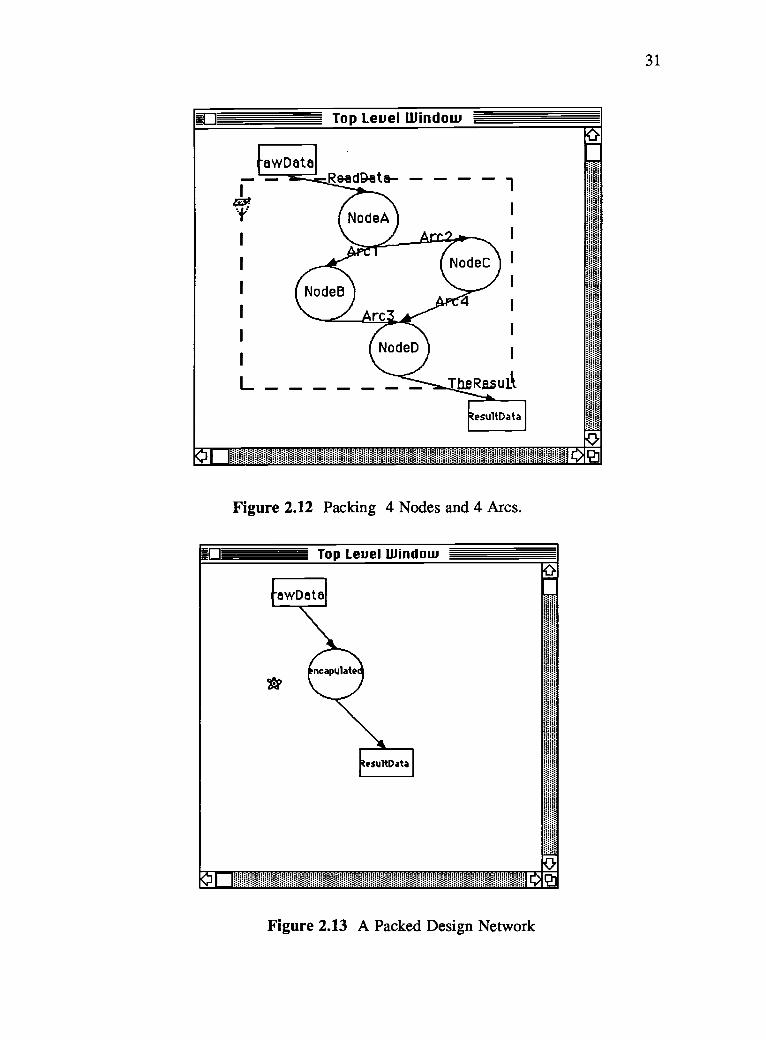
The pack tool is used to encapsulate a subnetwork of constructs into one compound

node. Consider the ELGDF network shown in Figure 2.12. To pack the subnetwork

made of NodeA, NodeB, NodeC, NodeD, Arcl, Arc2, Arc3, and Arc4, we draw a

selection box around the subnetwork as shown in the figure. Figure 2.13 shows the

design after packing. The original ELGDF design network can be obtained again using

the unpack tool. The go-down tool is used to get the constituents of a compound node in

a separate window. Figure 2.14 shows the new window created for the subnetwork of

the compound node "encapsulated". The bridge tool is used in connecting constructs in

different windows as shown in Figure 2.15.

31

-0 Top Leuel Window

-awDataReed Data

1

NodeA

rc

NodeD

LResultData

Figure 2.12 Packing 4 Nodes and 4 Arcs.

Top Leuel Window

awData

ResultData

iiiiiiiiiiiiiiiiiiiiiiiiiiiiiiiiiiiiiiiiiiiiiiiiiiiiiiiiiiiiiiiii C>

Figure 2.13 A Packed Design Network

Yes )

32

Top Leuel Window4

. : :i. :: :..,..,.:.::::ii

.li iiill

..1i ..i1.: ..11Il

I.i...-..:.;.:.:.,.:

:11111

-awDataencapulated

awData

NodeA

i

NodeC I

1 N odeB.

1 c3:

--.,,.

NodeD

TheResult

<3 L ...;....:.:.:.:.:.:.:::::::::.:1!::::::::::;;;I:i'd;i:::::::::::i:::::!:::!;fddifoifiii::::::::lifili:::::::::::::::::::::

Figure 2.14 A Subnetwork in a Separate Window Using Go-Down.

Top Leuel Window

awData

(Nod

Is this source symbol ?

Cancel No

A PI

-0 NodeB

odeCA elpstesultDa

odeBA

NodeCA

LIE

Figure 2.15 Connecting Two Nodes in Two Different Windows Using Bridge.

33

2.7 Summary

In this chapter, we have presented a graphical design language for parallel

programming. ELGDF serves as the foundation for a graphical design editor called

Parallax.

The complete syntax of ELGDF helps program designers deal with parallelism in

the manner most natural to the problem at hand. It allows the expression of the common

structures in parallel programs easily and compactly. For example the replication

mechanism used in ELGDF leads to a compact, flexible, and powerful representation of

dynamic graph structures.

In addition to expressing parallel programs in a natural way for both shared memory

and message passing systems, ELGDF provides a vehicle for studying parallel programs

by capturing parallel program designs for the purpose of analysis. ELGDF provides

design files that contain information needed by different tools in the PPSE.

The Parallax Design Editor provides a visual method of inputting software design

details in ELGDF notation. The following features have been implemented into Parallax:

1) ability to produce a hierarchical design for parallel software, 2) easy manipulation of

design by resizing, encapsulating, and expanding the graphical description, 3) ability to

assign source code fragments to specific graphical objects, and 4) ability to add detailed

textual specification to graphic notation through dialogues.

ELGDF has been used to design a parallel program which automate the process of

determining cloud properties from satellite image data. The graphical design and the

details of using the rest of the PPSE tools to produce parallel code are given in [Judg89].

34

Chapter 3

Static Mapping of Task Graphs with Communicationonto Arbitrary Target Machines

3.1 Introduction

The problem of scheduling parallel program modules onto multiprocessor

computers has received considerable attention in recent years. This problem is known to

be NP-complete in its most general form [Ullm75]. Regardless, many researchers have

studied restricted forms of the problem by constraining the task graph representing the

parallel program or the parallel system model [ChSh86, CoGr72, Linn85]. For example

when communication between tasks is not considered, a polynomial time algorithm can

be found for scheduling tree-structured task graphs wherein all tasks execute in one time

unit [Hu61].

It is well known that linear speedup generally does not occur in a multi-processor

system because adding additional processors to the system also increases inter-processor

communication [CHLE80]. In order to be more realistic we need to consider

communication delay in scheduling tasks onto multi-processor system. Prastein [Pras87]

proved that by taking communication into consideration, the problem of scheduling an

arbitrary precedence program graph onto two processors is NP-Complete and scheduling

a tree-structured program onto arbitrarily many processors is also NP-Complete.

Kruatrachue [Krua87] introduced a new heuristic based on the so called list algorithms

that considers the time delay imposed by message transmission among concurrently

running tasks by assuming a homogeneous fully connected parallel system.

35

Task allocation is not the same as task scheduling. The goal of task allocation is to

minimize the communication delay between processors and to balance the load among

processors [Bokh8la, Bokh8lb, ChAb81, Tows86]. Kruatrachue [Krua87] showed that

task allocation is not sufficient to obtain minimum run time since there is a significant

difference in performance when the order of execution is changed among allocated tasks

on a certain processing element. Other work has been done in task allocation when the

program is represented as an undirected task graph [Lo84].

Kruatrachue [Krua87] suggested some directions for future work in relaxing

restrictions in the program task graph and the parallel system model. In this chapter we

extend the parallel system model used by Kruatrachue to accommodate arbitrary parallel

systems. We introduce a mapping heuristic (MH) that maps program modules

represented as nodes in a precedence task graph with communication onto arbitrary

machine topology. MH gives an allocation and ordering of tasks onto processors.

Contention is considered in MH so that the route with less contention is always used for

communication. MH also keeps contention information in tables and updates them when

certain events take place so it can make the scheduling decisions based on a current traffic

state.

The significance of this work is that we can now do better at scheduling task graphs

onto multiprocessor systems by considering the target machine, communication delay,

contention, and the balance between computation and communication.

The rest of this chapter is organized as follows. List scheduling is briefly described

in section 3.2. Section 3.3 contains the formulation of the problem. Section 3.4 shows

the proposed mapping heuristic without considering contention. We extend our mapping

to handle contention in section 3.5. Section 3.6 contains some experimental results that

study the effects on performance of: 1) using different machine topologies and different

36

number of processing elements, 2) changing the policy used in MH to select a task, and

3) changing two parameters of the task graph when a hypercube is used as target

machine. We introduce "Task Grapher," a useful tool for scheduling parallel program

tasks in section 3.7. Finally, we finally give a summary in section 3.8.

3.2 List scheduling

One class of scheduling heuristics, which includes many parallel processing

schedulers, is called "list" scheduling. In list scheduling each task is assigned a priority.

Whenever a processor is available, a task with the highest priority is selected from the list

and assigned to a processor. The schedulers in this class differ only in the way that each

scheduler assigns priorities to nodes. Different priority assignment results in different

schedules because tasks are selected in different order. A comparison between different

task priorities has been studied in [ACDi74].

The insertion scheduling heuristic (ISH) and the duplication scheduling heuristics

(DSH) introduced by Kruatrachue [Krua87] are essentially improved list schedulers.

ISH considers "slots" created by considering the communication delay problem. An

insertion routine inserts tasks in available communication delay time slots. DSH uses

duplication of tasks to offset communication. A duplication routine is used to duplicate

the tasks that cause communication delay, thus increasing performance with little effort.

We introduce a new heuristic that modifies Kruatrachue's basic heuristic so it can

handle communication delay between tasks assigned to heterogeneous processing

elements in an arbitrary target machine topology, taking contention into consideration.

The insertion routine used in ISH as well as the duplication routine used in DSH can be

easily inserted into MH. We study the effect of interconnection topology on schedules,

and in turn, on the performance of the parallel program on a specific parallel processing

architecture.

37

3.3 Formulation of the Problem

Our goal is to devise an efficient heuristic scheduler to statically map parallel

program modules onto a fmite number of processing elements in a pattern that minimizes

final completion time as determined by actual task computation time and communication

between processors.

We first ignore contention in the network to illustrate the basic ideas behind the

heuristic. We assume for now that the communication channels have sufficient capacity

to service all transmission without significant delay due contention. In section 3.5 we

relax this assumption and introduce a version of the heuristic that can handle contention.

3.3.1 Program Graph

A parallel program consists of M separate cooperating and communicating modules

called tasks. Its behavior is represented by an acyclic directed graph called a task graph.

A directed edge (i,j) between two tasks i and j exists if there is a data dependency between

the two tasks which means that task j cannot start execution until it gets some input from

task i after its completion. Once a task begins execution, it executes until its completion

(non-preemption). The task graph is assumed to be static which means it remains

unchanged during execution.

3.3.2 Target Machine

A target machine is assumed to be made up of an arbitrary number N of

heterogeneous processing elements. The machine runs one application program at a time.

These processing elements are assumed to be interconnected in an arbitrary way. A

message sent from a task running on processing element Pk to another task running on

processing element P1 takes the shortest path between the two processing elements

38

through one or more hops. Communication time between two tasks located on the same

processing element is assumed to be zero time units. The term processing element is used

instead of processor to imply the existence of an I/O processor. A processing element can

execute a task and communicate with another processing element at the same time.

We define the following parameters associated with target machines:

H(ni,n2): minimum number of hops between processing elements ni and n2,

R(ni,n2): the transmission rate over the link (ni, n2), (n1, n2 are two adjacent

processing elements)

I(ni): the time to initiate message passing on the I/O channel with processing

element ni.

S(ni) gives the speed of processing element n1

We assume that the I/O processors are identical and take the same amount of time to

initiate a message ( I = I(ni), 0 ni < N). We also assume that the transmission rate is

the same all over the interconnection network ( R = R(ni,n2), 0 ni,n2 < N).

3.3.3 System Parameters

Parameters are required to represent the computational costs and communication

costs incurred by a parallel program on a specific parallel processing system. The costs

are as follows:

E(m,n): the execution time of task m when executed on processing element n,

lm 5. M; Oti < N.

39

C(ml,m2,nl,n2): the communication delay between tasks m1 and m2 when

they are executed on processing elements ni and n2, respectively, 1 rni,m2 .M;

(Xni, n2<N.

The parameter E(*) reflects the speed of the processing elements and the size of the

tasks. E(m,n) = INS(m)/S(n) where INS(m) gives the number of instructions to be

executed at task m and S(n) gives the speed of processing element n, 15.m1; 05_n<N.

The parameter C(*) reflects the target machine performance parameters as well as

the size of the data to be transmitted. Without considering contention, the parameter C(*)

can be obtained as: C(ml,m2,nl,n2) = (D(mi,m2)/ R + I)*H(ni,n2) where D(ml,m2)

gives the size of the data to be sent from m1 to m2, H(ni,n2) gives the number of hops

between ni and n2, I represents the time to initiate message passing on each processing

element, and R represents the transmission rate, 1 rni,m2 VI; 05_ni, n2<N.

The model studied by Kruatrachue [ICrua87] can be easily generated as a special

case of our model. He assumes a fully connected target machine with similar processing

elements.

Example 3.1

Figure 3.1 shows an example of a task graph consisting of 5 nodes (M = 5). The

number shown in the upper portion of each node is the node number, the number in the

lower portion of a node i represents the parameter INS(i), and the number next to an edge

(i,j) represents the parameter D(i,j). For example INS(1) = 10, D(4,5) = 1.

Figure 3.2 shows an example of a parallel system (target machine) consisting of 8

processing elements (N = 8) forming a cube of dimension = 3. Notice that H(0,7) = 3,

because a message sent from node 0 to node 7 takes three hops.

40

Figure 3.1 Example of Task Graph. Figure 3.2 Example of Target Machine.

3.4 The Mapping Heuristic (MH)

The mapping heuristic takes two inputs: 1) a description of the parallel program

modules and their interactions in the form of a task graph, and 2) a description of the

target machine in the form of a table. It produces as output a Gantt chart that shows the

allocation of the program modules onto the target machine processing elements and the

execution order of tasks allocated to each processing element. A Gantt chart consists of a

list of all processing elements in the target machine and for each processing element a list

of all tasks allocated to that processing element ordered by their execution time, including

task start and finish times. Figure 3.3 shows the Gantt chart resulting from scheduling

the task graph (TG1) on the target machine (TM1) of two similar processing elements.

41

Program Task (TG1)Graph

Target machine (TM1)

Mapper

30

P1 P2

2 1

34

Gantt Chart

11

31

36

Figure 3.3 Gantt Chart Resulting From Scheduling Task Graph (TG1) on Target

Machine (TM1).

3.4.1 Definitions

The length of a path in a task graph is the summation of all node execution times

and edge communication delays along the path. The level of a node is defined as the

length of the longest path from the node to the exit node.

Adam, Chandy, and Dickson [ACDi74] compared 5 different ways of assigning

priorities: HLFET (Highest Level First with Estimated Times), HLFNET (Highest Level

First with No Estimated Times), RANDOM, SCFET (Smallest CO-level First with

Estimated Times), and SCFNET (Smallest CO-level First with No Estimated Times). He

42

showed that among all priority schedulers, level priority schedulers are the best at getting

close to the optimal schedule.

Following [ACDi74], we use the level at each node as its priority. However, after

adding communication delay, the node level is not static and may change according to the

mapping. So far nobody has solved the level problem when communication delay is

considered [Krua87]. Some researchers simply ignore communication delays in

calculating the level at each node. We have studied both strategies for calculating the

level: 1) with, and 2) without communication. When we include communication in

calculating the level, we assume that all messages are sent through a one-hop channel

because the mapping is not known yet. The results of our study using hypercube target

machines is given in section 3.6.

The ready time of a processing element P (ready_time[P]) is the time when

processing element P has finished its assigned task and is ready to execute a new one.

The message ready time of a task (Time_message_ready) is the time when all messages to

the task have been received by the processing element running the task. The speed up is

defined as the program execution time when it runs on one processing element divided

by its execution time when it runs on a multi-processor system.

3.4.2 MH

The heuristic can be explained in the following three steps:

L The level of each node in the task graph is calculated and used as each node's priority

(in case of a tie we break it by selecting the one with the largest number of immediate

successors. If this does not break the tie, we select one at random). An event list is

initialized by inserting the event "task is ready" at time zero for every node that has no

immediate predecessors. Events are sorted according to the level priorities of their tasks,

with the highest priority task first.

43

II. Then, as long as the event list is not empty:

1) an event is obtained from the front of the event list.

2) If the event indicates that " task T is ready ", a processing element is selected to run the

task T, ( a processing element is selected in such a way that the task cannot finish on any

other processing element earlier). The selected task is then allocated to the selected

processing element, and at the time when the selected task will finish running on the

selected processing element, the event " task T is done " is added to the event list.

3) If the event indicates " task T is done " , the status of the immediate successors of the

finished task is modified. So when task T finishes execution, the number of conditions

that prevent any of its immediate successors from being run is decreased by one. When

the number of conditions associated with a particular successor becomes zero then that

successor node can be scheduled.

III. Step II is repeated until all the nodes of the task graph are allocated to a processing

element. (Figure 3.4 gives the detailed heuristic).

The event list is always sorted according to the time. The event that happens at the

lowest time comes first. The event list maintains two types of events: 1) event 1 indicates

that a task is ready and 2) event 2 indicates that a task has finished. When more than one

event of type 1 happen at the same time, they are sorted according to the priorities of their

tasks, yielding the highest priority task, first.

Example 3.2

Figure 3.5c shows the Gantt chart that results from using MH to schedule the task

graph given in Figure 3.5a on the hypercube consisting of 4 similar processing elements

given in Figure 3.5b.

44

beginLoad the program task graph.

Load the target machine.

Compute the level of each task.

Initialize the event_list (E).

while E is not empty do

beginget event (e) from E.

process_event (e)

end.end

Figure 3.4a The MH Algorithm.

procedure Initialize the event_list (E)

beginLet Source be the set of all tasks without immediate predecessors.

Let Source = ( ti, t2, ..., tm )

if Source is not empty then

for i := 1 to m doinsert _event ("task ti is ready" at time zero). (* event type = 1 *)

events are sorted according to the level priorities of their tasks,

yielding the highest priority task, first, followed by lower priority.

end.

Figure 3.4b Initialize Event List Routine.

45

procedure process_event (event);

begincase event type

= 1 (* " task T is ready " *)

schedule_task (1).

end.

= 2 (* " task T is done " *)

handle_successors (T).

Figure 3.4c Process Event Routine.

procedure schedule_task (T)

beginlocate_processor (T,P).

assign T to P.

Let fin_time be the finish time of task T on processor P.

insert _event ("task T is done" at time fin_time). (* event type = 2 *)

end.

Figure 3.4d Schedule Task Routine.

46

procedure handle_successors (T);

beginLet IMS be the set of all immediate successors of T.

Let fin time be the finish time of task T.Let IMS = { ti, t2, ..., tm } where ti has nri associated with, where nri is the

number of reasons that prevents ti from starting execution

(initially nri = number of immediate predecessors of task ti);

if IMS is not empty then

for i := 1 to m do

beginnri < nri - 1;

if nri = 0 theninsert _event ("task ti is ready" at time fm_time).

(* event type = 1 *)

end.end

Figure 3.4e Handle Successors Routine.

47

procedure insert_event (event)

begininsert event in the event list such that the event list is sorted according to the time

, yielding the lowest time event, first.

if more than one event happen at the same time then

beginthe events are sorted according to the their event types,

yielding the highest event type, first.

if events are of event_type =1

thenthe events are sorted according to the level priorities of their tasks,

yielding the highest priority task, first, followed by lower priority.

else

end.end

Figure 3.4f Insert Event Routine.

48

procedure locate_processor (T,P)

beginP <. k.

where finish_time(T,k) finish_time(T,i), 0 i < N

end.

Figure 3.4g Locate Processor Routine.

function finish_time(T,P)

beginLet IMP be the set of all immediate predecessors of T.

if IMP is empty thenfinish_time < ready_time[P] + E(T,P)

elseLet IMP = ( t1, t2, ..., tm )

where ti is assigned to processor p[ti].

Time_message_ready <-- max(ready_time[p[ti]]+ C(tj, T, p[ti], P)), 1 5_ i S m.

start_time < max(Time_message_ready, ready_time[P])

finish_time f- start_time + E(T,P)

end.

Figure 3.4h Finish Time Function.

49

time

(a)

processing elements0 1 2 3

(c)

(b)

9

11

24

26

Figure 3.5 (a) Task Graph, (b) Hypercube Target Machine, and (c) the Resulting

Gantt Chart.

50

3.4.3 Complexity Analysis

Let M be the number of tasks in the task graph, and N be the number of processing

elements in the target machine. The worst case time complexity of MH can be obtained as

follows.

Compute level: 0(M2)Complexity is related to the number of edges in the task graph which is 0(W).

Initialize event list: 0(MlogM)At most M events are sorted.

Get an event from the event list: Constant

The event on the front of the list is taken in constant time.

Locate processor: 0(N*M)Since finish-time function of task T on processing element P considers thecommunication delay caused by all immediate predecessors of task T, then its worst

case complexity is 0(M). The locate-processor routine calls finish-time Ntimes so the complexity is 0(N*M).

Schedule task: 0(N*M)It calls locate processor which is 0(N*M).

Insert event: 0(M)Each task causes two events to be added to the event list which is 0(M).

Handle successors: 0(M)Since handle successors considers all immediate successors of a task then the worst

case complexity would be 0(M).

Process event : 0(N*M)Since it calls either schedule task or handle successors..

51

The while loop in MH (Figure 3.4a) is executed 2*M times. The shortest path from

any processing element to every processing element can be done in 0(N3). The

complexity of MH is 0(M2+MlogM+M2+N*M2+N3), which is 0(N*M2+N3). That

means the time complexity is 0(M2) for constant number of processing elements.

3.4.4 Correctness of MH

We now show that the heuristic is correct in the sense that it schedules all tasks in

the task graph on the available processing elements, and terminates. This follows if every

task becomes ready exactly once. As shown in Figures 3.4(c&d), if the current event

shows that a task is ready then it will be scheduled on some processing element. Having

each task become ready exactly once guarantees the termination of the program.

Suppose that the event that "task T is ready" is not inserted into the event list at all.

Let parent(T) be a function that returns the set of all immediate predecessors of task T. If

parent(T) is empty then task T is a source node and its readiness event must have been

inserted to the event list in the initialization routine; which leads to contradiction. If

parent(T) is not empty then there must be at least one immediate predecessor (PT E

parent(T)) such that its readiness event has not been inserted into the event list at all

which means that at least one element of parent (PT) has not been ready which eventually

leads to a source node that has not been ready and again that leads to contradiction. We

conclude that the readiness events for all tasks are inserted at least once to the event list.

Suppose that the event that "task T is ready" is inserted to the event list more than

once and suppose that the number of reasons that prevents T from getting scheduled is

nr(T). Initially nr(T) = I parent(T) I and whenever an element of the set parent(T) is

scheduled nr(T) is decreased by one. Since nr(T) is set to I parent(T) I only once so it

52

reaches zero only once and T cannot be scheduled more than once. So using MH, every

task is inserted to the ready queue exactly once.

3.5 Considering Contention in MH

Systems in which multiple users share a common channel in a way that can lead to

conflicts are widely known as contention systems [Tane81]. For example when a parallel

program runs on a message-passing multi-processor system, contention happens when

two (or more) parallel tasks of the program running on different processing elements send

messages through one or more common channels. Contention also happens on a shared-

memory system when two (or more) processors need the shared bus at the same time.

Contention leads to delaying the arrival of messages to their destinations.

In the previous section, we assumed that the communication channels had sufficient

capacity to service all transmissions without significant delay due to contention. In this

section we introduce the necessary modifications to the mapping heuristic MH so that it

can handle contention.

3.5.1 MH Modifications

We modify MH to achieve three goals: 1) to include delays due to contention in the

communication parameter C(*), 2) to find heuristically routes with lower communication

delays, and 3) to produce more realistic schedules.

The modification to MH takes place in the way we compute the communication

delay between tasks running on different processing elements and in having two more

events in the process event routine for updating contention information. However the rest

of the heuristic remains the same.

53

For each processing element in the system, we maintain a routing table that has

contention information indexed by, and containing one entry for, each other processing

element. This entry contains three parts: 1) the number of hops (h), 2) the preferred

outgoing line to use for that destination (1), and 3) the communication delay due to

contention (d).

Initially, we use the shortest path between any two processing elements to

determine the number of hops (h) and the preferred outgoing line (1). If we have more

than one shortest path we just pick any one randomly. The delay (d) is assigned zero.

We are going to use hpi, pi to refer to the number of hops between processing elements

pi, pi (could be longer than the shortest path). Also !pi, pi, and dpi, pi are going to be

used similarly.

Figure 3.6 shows a muliprocessor system with four processing elements forming a

ring (cube) and the initial tables for the four processing elements. For example the value

of li, 2 is 3 as shown from the table associated with processing element 1.

0

h 1 d

1

hl d

(a)

2 3

h i d h1 d

54

0 0 - 0 1 0 0 1 0 0 22 0

1 1 1 0 0 0 2 0 0 11 0

2 1 2 0 2 3 0 0 0 120

3 2 1 0 1 3 0 1 3 0 0 0

(b)

Figure 3.6 (a) Target Machine With 4 Processing Elements, and (b) the Initial Tables

Associated With Each Processing Element.

The tables maintained for each processing element are used to obtain the "best"

route to send a message and to compute communication delay which guides the selection

of the best processing element for a certain task. The parameter C(mi,m2,ni,n2)

represents the communication delay between tasks m1 and m2 when they are executed on

processing elements n1 and n1, respectively, 1 m1, m2 5 M; 0 n1, n2 N-1. Two

time delays contribute to the communication delay: 1) the time delay incurred in

transmitting data from m1 to m2 over an empty route between n1 and n2, and 2) the

queuing delay (contention) due to multiple messages sent through the route between n1,

n2.

55

The first time delay due to transmission can be obtained as: (D(mi ,m2)/

R+I)*hn1,n2, where D(m1,m2) is the data size to be sent from m1 to m2 and hill, n2 is the

number of hops between n1 and n2. The parameters R and I represent the transmission

rate and the time to initiate message passing on each processing element respectively. The

other time delay due to contention can be obtained from the table associated with

processing element n1 as: 41, n2. So the parameter C(m1,m2,n1,n2) used in the

algorithm given in section 3.4.2 is computed as follows:

C(m1,m2,n1,n2) = (D(m1,m2) / R + I) * hill, n2 + dill, n2

3.5.2 Adaptive Routing

The tables maintained for each processing element are updated during scheduling so

that the decisions made in choosing a route to send a message or selecting a processing

element to run a task are based on information about the current traffic. Now three

questions need to be answered: 1) when are tables updated?, 2) which tables are

updated?, and 3) how?

To answer these question we should keep in mind that the more often we update the

tables the better view of the current traffic we get and the more expensive it gets. There is

a trade off between having a real view of the traffic and the complexity of the update

procedure. We update the tables when either of the following two events happens during

scheduling: 1) a task starts sending a message to another task, 2) a message arrives at its

destination. The first event is important because it keeps communication routes busy

during transmission. The second event is important because it frees a route for sending

messages by other processing elements in the system.

Suppose that IMP = (ti, t2, ..., tm} is the set of all immediate predecessors of task

v, where ti is allocated to processing element p[ti] and processing element p[v] is chosen

56

to run task v. Table update takes place when either of these two events happen. The first

event is when task ti on processor p[ti] (1 i m) has finished and starts to send its

message. The second event happens when the message sent from task ti on p[ti] has

arrived at its destination. We perform the update twice for each arc in the task graph (

0(M2) ), where M is the number of tasks in the task graph. Recall that in a dataflow-like

model, each arc is used only once.

Not every table is updated. Only the tables associated with the processing elements

on the routes where traffic status is affected as a result of having one or more messages

occupying some (or all) of the channels on those routes. Tables are updated only once.

Tables of processing elements on the communication route are updated first (Direct Effect

on the Route) then the tables of the neighbors that have been affected and have not been

updated yet are updated (Indirect Effect on Neighbors). Each time we do the update, at

most N tables are updated where N is the number of processing elements in the target

machine.

We update at most N tables, M*(M-1) times in the worst case, where M is the

number of tasks in the task graph and N is the number of processing elements. And since

each table has N entries, the complexity of the table update part is 0(N3*M2). The

complexity of MH considering contention is 0(N3* m2+ N*m2+N3), which is 0(M2) for

a constant number of processing elements.

Two routines are modified to handle contention. Process_event routine is modified,

as given in Figure 3.7, to handle two more event types: 1) event 3 which indicates that a

task starts to send a message and 2) event 4 which indicates that a message has arrived at

its destination. Schedule task routine has also been modified so it can update the event

list when any of the two new events happens, Figure 3.8 shows the modified routine.

57

The rest of the routines have not been changed. Updating the tables according to events 3

and 4 are given in sections 3.5.2.1 and 3.5.2.2, respectively.

procedure process_event (event);

begincase event type

= 1 (* " task T is ready " *)

schedule_task (T).

end.

= 2 (* " task T is done " *)

handle_successors(T).

= 3 (* " a message needs to be sent from pi to p2 " *)

update tables according to event 3.

= 4 (* " a message sent from pl has arrived at p2 " *)

update tables according to event 4.

Figure 3.7 Process Event Routine (with contention).

58

procedure schedule_task (T)

beginlocate_processor (T,P).

assign T to P.

Let fm_time be the fmish time of task T on processor P.

insert _event ("task T is done" at time fin_time). (* event type = 2 *)

Let IMP be the set of all immediate predecessors of T.

if IMP is not empty thenLet IMP = ( t1, t2, ..., tm )

where ti is assigned to processor p[4].

Let fi be the finish time of ti on p[ti], and

ai is the arrival time of the message sent from ti on p[ti] to T on P.

for i := 1 to m dobegin

insert _event (" a message should be sent from p[ti] to P " at time fi).

(* event type = 3 *)insert event (" a message sent from p[tit] has arrived at P " at time at ).

(* event type = 4 *)

end.end

Figure 3.8 Schedule Task Routine (with contention).

59

3.5.2.1 Event _3 Update

Direct Effect on the Route (Event 31

Suppose that task t1 on processing element p1 sends a message to task t2 on

processing element p2. All tables of processing elements on the route from p1 to p2

except p2 are updated according to the algorithm given in Figure 3.9a. The table

associated with processing element p2 is not updated because the route from p2 to other

processing elements has not been affected.

Procedure Direct_Effect_on_the_Route_Event_3

beginLet task t1 on 131 sends a message to t2 on 132

transmission < (D(ti,t2) / R+ I).

Update_Delay (transmission,p1,p2,3, delay)

end

Figure 3.9a Direct_Effect_on_the_Route_Event_3.

60

procedure Update_Delay (transmission,p1,p2, event, var delay)

beginif ip 1 p2 = p2 then

beginif event = 3 then delay 4- dp1, p2 + transmission.

else delay 4- dp 1, p2 transmission.

dp1, p2 4 delay

endelse

beginUpdate_Delay (transmission,p1,1pi, p2, event, delay1)

Update_Delay (transmission,lpi, p2,p2, event, delay2)

delay 4 delay1 + delay2

end

dp b p2 4 delay

end

Figure 3.9b Update_Delay Routines.

0 1

h 1 d h 1 d

0 0 0 1 0 0

1 1 1 5 0 0

2 1 2 0 2 3 0

3 2110 1 3 5

Figure 3.9c Tables 0 and 1 After the Direct Effect Update.

61

Example 3.3

Consider the target machine given in Figure 3.6. Suppose that task ti is assigned to

processing element 0 (pi = 0) and task t2 is assigned to processing element 3 (1)2 = 3),

and D(ti,t2 ) = 5. Also assume that R = 1 and I = 0. Using the algorithm given in

Figure 3.9a, tables 0 and 1 are updated. Figure 3.9c shows tables 0 and 1 after update.

Indirect Effect on Neighbors

The tables of the neighbors of processing elements with updated tables are updated

according to the algorithm given in Figure 3.10a.

procedure Indirect_Effect_on_Neighbors.

beginLet A be the set of all neighbors of pi.

Pnext 4 1P14:02

Ai < A {Pnext)enqueue all elements of A' in Q.

while Q is not empty do

begindequeue (Q,p) (* get p from the front of Q *)

if the table associated with p has not been updated yet

thenbegin

Let A" be the set of all neighbors of p.

Update_Neighbors(A",p).

enqueue all elements of A" in Q.

endend

end

Figure 3.10a Indirect_Effect_on_Neighbors.

62

procedure Update_Neighbors (A,p)

beginLet A = {al, a2,..., ab).

for i := 0 to N-1 do

begindo dp,ak + dakj

10 < ak.ho 4-- 1 + hao ,

where dp,ak + dak,i

endend

dmi + dap , 1 j 5_ b.

Figure 3.10b Update_Neighbors Routines.

Example 3.4

Consider the target machine given in Figure 3.6 after the direct effect update as

shown in Figure 3.9c. As given in Figure 3.9c only tables 0 and 1 have been updated

after direct effect update. Now we do the indirect effect on the neighbors of processing

element 0. It can be noticed that p1 ' 0 , Pnext = 1, A = ( 1,2), A' = (2), and Q will

have only one element 2. Processing element 2 needs to modify its table according to

information from its neighbors, processing elements 0 and 3. Figure 3.10c shows the

tables associated with the neighbors of processing element 2 (0 and 3) and the new table

for 2. It can be noticed that d2,0 = 0 and d2,3 = 0. Consider how the new route from 2 to

1 is computed. Processing element 2 knows it can have d2,1 = 5 (5+0) if it takes the

route passing by 0 or d2,1 = 0 (0+0) if it takes the route passing by 3. The best of these

two values is 0 of course, so we update the route to go through 3.

63

0 3 2

h i d h i d h 1 d

0 0 - 0 2 2 0 1 0 0

1 1 1 5 1 1 0 2 3 0

2 1 2 0 1 2 0 0 0

3 2 1 10 0 0 1 3 0

d 2,0 = 0 d 2,3 = 0

Figure 3.10c Input From 0, 3 and the New Table for 2.

3.5.2.2 Event _4 Update

Direct Effect on the Route (Event 4)

Suppose that the message sent from task t1 on processing element p1 to task t2 on

processing elements p2 has already arrived. All the tables of the processing elements on

the route from p1 to p2 except p2 are updated according to the algorithm given in Figure

3.11.

Procedure Direct_Effecton_the_Route_Event_4

beginLet a message from t1 on p1 to t2 on p2 has already arrived

transmission <--- (D(t1,t2) / R+ I).

Update_Delay (transmission,p1,p2,4, delay)

end

Figure 3.11 Direct_Effect_on_the_Route_Event_4 Routine.

64

Indirect Effect on Neighbors

The tables of the neighbors of processing elements with updated tables are updated

according to the same algorithm given in Figure 3.10a.

Example 3.5

Consider the target machine given in Figure 3.6 after reflecting the direct effect

update and the indirect effect on neighbors as shown in examples 3.3 and 3.4. Now

suppose that task t2 on processing element 3 has already received its message from task

ti on processing element 0 and is about to start execution. Now it is time to update the

tables according to "Event_4 Update" which produces the original tables given in Figure

3.6b with the only difference that in the table associated with processing element 2 the

route from 2 to 1 goes through 3 instead of 0 as explained in example 3.4.

65

3.5.3 How Good is MH?

When all tasks of a task graph are of unit duration and communication between

tasks is not considered, it is known that there are polynomial time algorithms for finding

the optimal schedules in two restricted cases: 1) the target machine consists of two similar

processors [CoGr72], or 2) the task graph is a tree [Hu61].

Prastein [Pras83] proved that when communication is considered the problem with

two similar processors when all tasks are of unit duration is NP-complete. The problem

with a fully connected target machine with similar processors on a tree task graph with all

tasks are of unit duration is also NP-complete.

Considering communication in those restricted cases makes it very hard to find the

optimal schedules. Scheduling arbitrary task graphs on fully connected homogeneous

target machines makes it even harder [Gonz77, Pras83].

The goal for MH was to find a suboptimal schedule for a more general case which

is even harder. MH considers: 1) tasks with different execution times, 2) variable

communication times between tasks, 3) contention in the network, and 4) the network

topology.

To find out how good MH is, one might need to express MH in terms of bounds.

That is, the schedule which results from the heuristic MH is expressed as a ratio that

compares the suboptimal schedule to the optimal schedule. We identify the general case

as an open research problem. For some restricted forms of the task graph and the target

machine, MH can be expressed in terms of bounds. Let ETA be the total execution time

produced by MH and ET° be the the total execution time with an optimal schedule. FormH

comparison, we will let R be the ratioETET0

66

Case 1: M arbitrary independent tasks forming a task graph and N similar

processors forming a target machine. In this case MH uses HLF (highest level first)

which has been also called LPT (longest processing time) rule and R would be bounded4 1by 3 - Tg [HoSa78].

Case 2: M arbitrary tasks forming a precedence task graph with no communication

and two similar processors forming a target machine. In this case MH uses HLF (LPT)4

and R would be bounded by 3 [ChLi74].


and three similar processors forming a target machine. In this case MH uses HLF (LPT)3



and N similar processors forming a target machine. In this case MH uses HLF (LPT)


Without enumerating all possible solutions and then selecting the best one, the

optimal solution cannot be found. For problems with a small number of possibilities,

enumeration may not be especially difficult. However, when the possibilities are very

large the exponentially increasing computational time required to enumerate all possible

solutions enhances the attractiveness of heuristic approaches. Since there are many

factors to be considered in MH, finding the optimal solution can take a great amount of

time. Thus we think that a thorough assessment of MH by experimentation will require

extensive computations. We leave this problem for future work. However, we compare

the schedules generated by MH and the optimal ones for some task graphs in following

example.

67

Example 3.6

In this example, we schedule some task graphs using MH. We also find the

optimal schedules and compare them with those produced by MH.

Figure 3.12 shows the MH and the optimal schedules resulted from scheduling

seven independent tasks on three processors. Figure 3.12c shows the MH schedule.

This has a finish time of 11. Figure 3.12d shows an optimal schedule. Its finish time is11

9. Hence, for this instance R = v.

In Figure 3.13, we schedule a task graph with dependencies among the tasks but

there is no communication between tasks. The target machine has two processors. For

this instance MH produced an optimal schedule. Its fmish time is 14 and R = 1.

In Figure 3.14, a task graph with communication between tasks is scheduled on

four processors forming a cube. In this case MH produced an optimal schedule.

Figure 3.15 shows the MH and the optimal schedules resulted from scheduling a

task graph with communication on two processors. Figure 3.15c shows the MH

schedule. This has a finish time of 27. Figure 3.15d shows an optimal schedule. Its27finish time is 23. Hence, for this instance R = -. In Figure 3.16, we use a task graph

similar to the one used in Figure 3.15 with some changes in the task and message sizes.25

In this case MH did better and R = 23'

In Figure 3.17, we schedule a task graph with communication on four processors

forming a cube. For this instance MH produced an optimal schedule. Its finish time is

27. Figure 3.17d shows an optimal schedule that used only two processors. Figure 3.18

shows the change in the schedules after increasing the size of task 5 to 15 instead of 10.32

In this case R = T7.

0

4

5

8

11

(a)

PO P2 P3

31 2

46 5

(c)

0

5

9

(b)

P0 P1 P2

51 2

6

3 47

(d)

68

Figure 3.12 (a) Task Graph, (b) Target Machine, (c) MH Schedule, and (d) Optimal

Schedule.

(0)

pill,

Qt1N

01,14

1%"11:c

(t)

(9)

veltt

eti.

(a)

0

5

7

17

22

32

37

PO P1 P2 P3

................

':::::::.

%.. .

3

4 2

56

rr.rTnT:y:yi..-':'

-:...............;7

8

(c)

9

11

2426

(b)

70

Figure 3.14 (a) Task Graph, (b) Target Machine, and (c) MH Schedule (Optimal).

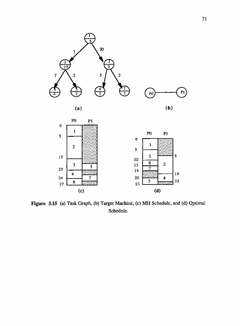
0

5

15

20

24

27

(a)

PO P1

1

2

3 5....-...,...........-...

76

(c)

0

5

10

13

16

20

23

(b)

PO P1

1

3

72

4

(d)

8

18

22

71


Schedule.

0

5

15

23

25

(a)

PO P1

1

2

3

4 5

6

(c)

17

20

0

5

15

23

PO

(b)

P1

1

2

3

7

4 5

6

(d)

10

17

20

72


Schedule.

0

5

10

15

20

25

27

(a)

PO P1 P2 P3

1 2 3 4

....

...

.....

....

....

...

....

::

6

....

...

.

. ........7

(c)

0

5

10

20

25

27

(b)

PO P1 P2 P3

1 3

2 4

5 6

........:::: . ..

.....:%:..:...........7

(d)

73


Schedule.

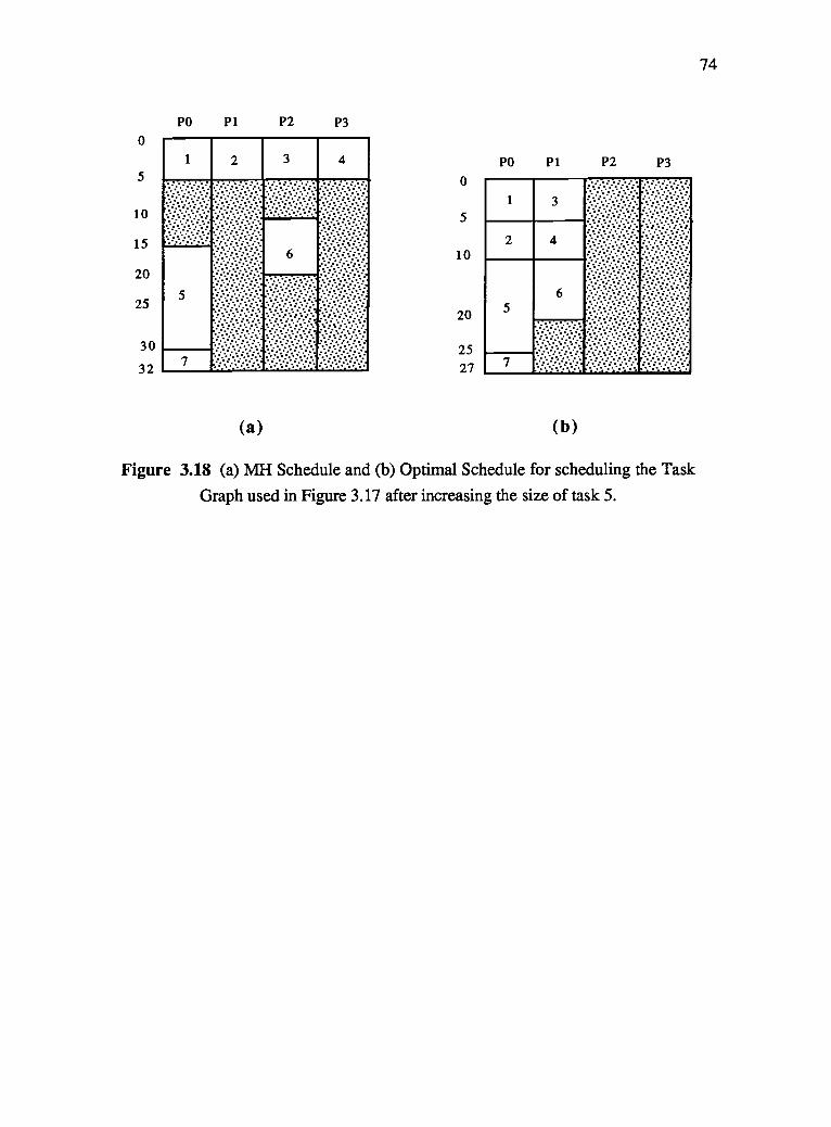
74

0

5

10

15

20

25

30

32

PO P1 P2 P3

1 2 3 4

6

5

7

(a)

0

5

10

20

2527

PO P1 P2 P3

1 3

2 4

65 ----..../

.6./..V..':.:::

(b)

Figure 3.18 (a) MH Schedule and (b) Optimal Schedule for scheduling the Task

Graph used in Figure 3.17 after increasing the size of task 5.

75

3.6 Simulation Results

In this section we show the simulation results of experiments conducted using the

MH mapping algorithm. The first experiment shows the change of the speed up as a

result of changing the target machine topology or the number of processors when running

various task graphs. The other two experiments study the effect of changing the policy

used in MH to select a task and of changing two parameters of the task graph representing

the parallel program on the performance when a hypercube is the target machine .

3.6.1 Experiment 1

This experiment studies the effect of changing the number of processing elements in

different target machine topologies on the speed up (defined in section 3.4.1). We used

MH to schedule varieties of task graphs ranging from communication intensive to

computation intensive graphs and from heavily dependent to lightly dependent ones on

five different target machines (with different numbers of processing elements): 1) fully

connected, 2) hypercube, 3) mesh, 4) star, and 5) ring. Figure 3.19 shows the average

speed up curves that result from scheduling 25 randomly generated task graphs, with

average number of nodes = 60, average number of edges in the range (25 - 100), average

execution time in the range (10 100) time units, and average amount of data at each arc

in the range (10 - 100) data units, on the five target machine topologies with transfer rate

= 1 and number of similar processing elements in the range (2 - 64).

From Figure 3.19 we can see that hypercube perform better than mesh, star, and

ring networks, but are not as well as fully connected networks. This is not surprising,

and indeed, the performance of a hypercube as compared with a fully connected network

is comparable according to our study.

12

10 -

8 -

6 -

4

2

00

-CI- cube- fully connected-13- ring

star-s- mesh

20 40

n_p rocesso r

Figure 3.19 Speed_Up Curves for 5 Different Target Machines.

3.6.2 Experiment 2

60 80

76

This experiment shows the effect of using communication delays in calculating the

level at each node in the MH algorithm. We generated 400 random graphs with average

number of nodes = 50, average number of edges in the range (25 100), average task

execution time in the range (10 - 100) time units, and average size of data at each arc in

the range (10 100) data units. We ran each graph on hypercubes of size 2, 4, 8, 16 ,

32, and 64 similar processing elements. As shown in the pie chart given in Figure 3.20

we found that 52.6% of the time using communication delays in calculating the level is

better than not using them. The performance was observed to be the same 10.8% of the

77

time. We also found that 36.6% of the time not using the communication delays in

calculating the level is better.

In the cases where using communication in calculating the level was better than not

using it, most task graphs were "communication intensive" (see Figure 3.21). It was also

found that most of the tasks were "execution intensive" when not using communication

was better (see Figure 3.22).

The results of experiment 1 suggests that for communication intensive applications,

the scheduler should consider communication delay in the scheduling algorithm's

priority, however for computation intensive applications, priority scheduling is

insensitive to the communication delays of the application.

52.6% of the runs better

10.8% of the runs same

36.6% of the runs worse

betterEl same0 worse

Figure 3.20 Using Communication in Calculating the Level in MH.

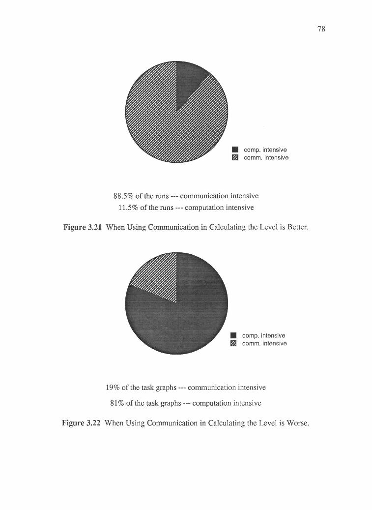
78

comp. intensiveEl comm. intensive

88.5% of the runs communication intensive

11.5% of the runs --- computation intensive

Figure 3.21 When Using Communication in Calculating the Level is Better.

comp. intensiveEa comm. intensive

19% of the task graphs --- communication intensive

81% of the task graphs --- computation intensive

Figure 3.22 When Using Communication in Calculating the Level is Worse.

79

3.6.3 Experiment 3

This experiment shows the effect of varying different program task graph

parameters on the performance. We chose two task graph parameters: the average degree

and the C/E_ratio, defined as follows:

number of edgesAverage degree number of nodes'

Average C/E ratioaverage communication delay between nodes

node average execution time

We generated 100 random graphs at each average C/E_ratio point in (0.1, 0.5, 1.0,

2.0, 10.0) and each average degree point in (0.5, 1.0, 1.5, 2.0). We ran each graph on

hypercubes of size 2, 4, 8, 16 , 32, and 64 similar processing elements. Figure 3.23

shows the speed up curve at each C/E_ratio and Figure 3.24 shows the speed up curve at

each degree.

The two sets of curves show the degradation in performance when the average

communication delay between program tasks begins to dominate the average task

execution time or when the number of edges in the task graph which represents the

number of interactions among tasks dominates the number of tasks in the program. The

curves also show that as the number of processing elements in the hypercube increases,

the degradation of performance due to the increase in the C/E_ratio or the graph average

degree is larger.

It can also be noticed that the average degree parameter is a good indicator of the

amount of communication in the task graph. For example the performance when the

average degree was 2 is comparable with the performance when the C/E ratio was 10.

80

The average degree can be used as a guide for MH in deciding when to use the

communication in computing the level in the task selection portion of the algorithm.

o.m

1.0

-0- C/E_ratio = 1 0- C/E_ratio = 2-II- C/E_ratio = 1-40- C/E_ratio = 0.5

C/E_ratio = 0.1

n_processor

Figure 3.23 The Effect of Changing the Communication-Execution Ratio on the

Speed_Up Curves when Using Different Hypercubes as Target Machine.

0-=

10-to

12

10-

8

6 -

4

2 -

0

-13- avg deg = 0.5

-*- avg deg =1

41- avg deg = 1.5

-o- avg_deg =2

, I 1

0 20 40 60

n_p rocesso r

80

81

Figure 3.24 The Effect of Changing Task Graph Average Degree on the Speed_Up

Curves when Using Different Hypercubes as Target Machine.

82

3.7 Task Grapher : A Tool for Scheduling Parallel Program Tasks

In this section we describe a tool for studying various approaches to scheduling

and its effect on system performance [Fort89, Su89]. Because we believe that different

heuristics apply to different kinds of problems, we are led to the conclusion that the best

solutions are obtained in cooperation with a human designer. Task Grapher is a tool to

answer "what if..." questions about a parallel program design, and to provide information

that can be used to fine-tune a design before it is actually run on a parallel computer.

3.7.1 Task Grapher -- The Tool

Task Grapher is a software tool which aids in parallel program design by

automating a number of scheduling heuristics and performance analysis tools. Task

Grapher produces: 1) schedules in the form of Gantt Charts for a number of scheduling

algorithms, 2) performance charts in the form of line and bar graphs, and 3) critical path

analysis.

With Task Grapher, a user can: 1) model a parallel program as a task graph

consisting of n tasks ( one task per node ), 2) choose a method of optimization from

several scheduling heuristics which will automatically schedule tasks onto m processors,

3) choose the topology of the desired target machine ( or design an arbitrary topology for

the parallel processor of interest, and 4) observe anticipated scheduling and performance

estimates obtained from the mapping of task graph onto target machine.

First, we describe the inputs and outputs of Task Grapher by way of an example.

Then we briefly describe the algorithms used to compute each output. For a detailed

description of these algorithms, consult the references.

File Edit Schedule Machine Analyze Layout

83

4-09-0 RTG1

/31

V3/

pirig, P.P.:: ......... . ::1041,;1.1=, I

Figure 3.25 A Task Graph Consists of Nodes and Arcs. The Integer in the Upper

Portion of Each Node is the Node Number. The Integer in the Lower Portion is an

Execution Time Estimate. The Arcs are Labeled with a Communication Message Size

Estimate.

A parallel program is represented as a task graph as shown in Figure 3.25. Each

node represents a task -- nodes are numbered, and they are assigned an estimate

representing the execution time for the task. Each arc represents an information flow

from one task to another. The arcs are labeled with an estimate of the size of the message

transmitted from node to node -- this number can be converted into a communication time

delay estimate once the performance of the interprocessor communication link is known.

Task execution time can vary from node to node, and communication arcs can be

labeled with any positive value. However, not all heuristics use this information in

computing a schedule. For example, the algorithm proposed by Hu [Hu61] ignores

communication delay estimates, see Figure 3.26.

84

Task graphs can be entered manually, using the drawing and editing tools shown in

the palette ( see Figure 3.25 ). The tools : 1) move nodes, 2) erase nodes and arcs, 3)

allow text to be entered numbers and labels, 4) create a node, and 5) create an arc.

The graphs can also be generated from other tools, which are not described here.

Task Grapher is part of a larger parallel program support environment which incorporates

computer-aided software engineering support for parallel programming [Lewi89]. When

automatically generated, task graphs correspond with actual code for implementing each

task. This information can be used to generate some of the timing estimates

automatically.

* File Edit Schedule Machine Analyze LayoutRTG I .HU

2 3 4 5 6

Time0

1

2

3

4

5

6

7

9

10

11

12'UF

17

5M:13£1131108V1f1MMRSISEWASMOWNMS11WWWWWWW1M38%*11'1121.M11M111W11110171513M73'74, 51M1::fi:VMS

Figure 3.26 Gantt Chart Produced by Task Grapher. Processor Numbers are Shown

Across the Top, and Time is Shown Down the Left Side. Light Shaded Regions Show a

Task Waiting for Communication, and Dark Shaded Regions Show When Tasks

Execute.

85

After a task graph is entered, various functions can be performed on it. The main

purpose is to compute schedules using one or more algorithms. We want to know which

schedule is "best", and we want to ask various "what if..." questions. For example,

what is the schedule computed by the algorithm proposed by Hu [Hu61]?

Figure 3.26 shows a schedule computed by Task Grapher for the n=11 node task

graph given in Figure 3.25, using the algorithm proposed by Hu [Hu61]. This schedule

assumed m=6 processors which are fully connected, but the program designer might ask,

"what if there were 16 processors?"

Any number of processors can be selected, and a corresponding Gantt Chart

computed, but a more insightful display is a speed-up line graph which compares the

expected performance improvement versus the number of processors employed. A

speed-up chart can be generated by computing schedules for each of the algorithms while

varying the number of processors from 1 to m.

Figure 3.27 shows a speed-up line graph which compares six algorithms for

scheduling up to six fully connected processors. (Speed-up is defined in section 3.4.1).

a File Edit Schedule Machine Analyze Layout

86

2.752.502.25

e 2.00d 1.75U 1.50

P 1.251.000.75

1 3 4Number of Processors

DSH K3 ISH 13K1 °YUD *HU

11>

Figure 3.27 Speed-Up Line Graph of the Task Graph Given in Figure 3.25 for a Fully

Connected Parallel Processor System. Six Scheduling Algorithms Yield Three Different

Schedules.

The performance of a parallel program represented as a task graph is influenced by

the interconnection topology of the parallel processors. Figure 3.28 shows the topology

of the fully connected system used to obtain Figures 3.26 and 3.27, for example. In

general, tree, mesh, toroid, and hypercube topologies are of interest. In addition, we

would like to ask "what is the effect on expected speed-up if the underlying topology is

changed?" This question is answered by selecting an alternate topology, or by manually

drawing an arbitrary network on the screen and producing a new speed-up line graph.

r St File Edit Schedule Machine Analyze Layout-El Untitled

87

16

... ::: : N '; iiiiiiiiiiiiiiiiiiiiiiiiiiiiiiiiiiiiiijahMilan0511111:011:11:1:111111:11111:11:111111=1:11111:1101:1:1

Figure 3.28 Fully Connected Interprocessor Connection Topology. Any Connection

Topology can be Evaluated by Entering the Topology into this Screen.

Finally, feedback from the analysis is used to improve the performance of a parallel

program design. A variety of performance measures can be used to discover what

hinders greater performance. But, the feature of greatest interest to a designer will be the

path of greatest delay, e.g. the critical path through the task graph.

A critical path in a task graph is a path from the beginning node to the terminating

node, which represents the longest execution delay. This is the portion of the program

containing the greatest opportunity for improvement. Figure 3.29 shows how Task

Grapher displays a critical path. The tasks and arcs along this path are candidates for

tuning.

r ö File Edit Schedule Machine Analyze LayoutRTG I .HU

88

OPP

nY.14:00giii4E0iEgpliggilggegOgilpipOggqpg!!A:gpOpg0gggOggggim:Egg0PwiEggg;Iggilii:pagiJiw*m0:4;mg:

Figure 3.29 Critical Path in the Task Graph of Figure 3.25 The Shaded Nodes Show

Which Nodes Lie Along the Path of the Greatest Execution Time.

3.7.2 Task Grapher Heuristics

In Task Grapher, programs must be represented by an acyclic-directed task graph

TG(N,E) [Krua87], where N is a set of numbered nodes representing tasks submitted to

the system and E is a set of edges representing ordering restrictions among the tasks.

Each node is given a value, or "size", equal to the execution time of the task. Each edge

is given a value equal to the size of the message delivered from one node to another.

Given the target machine characteristics, the communication delay time due to delivery of

a message from one node to another can be easily obtained. The communication delay

time between two tasks is assigned a value of zero when both tasks are allocated to the

same processor, and it is non-zero when tasks are assigned to different processors.

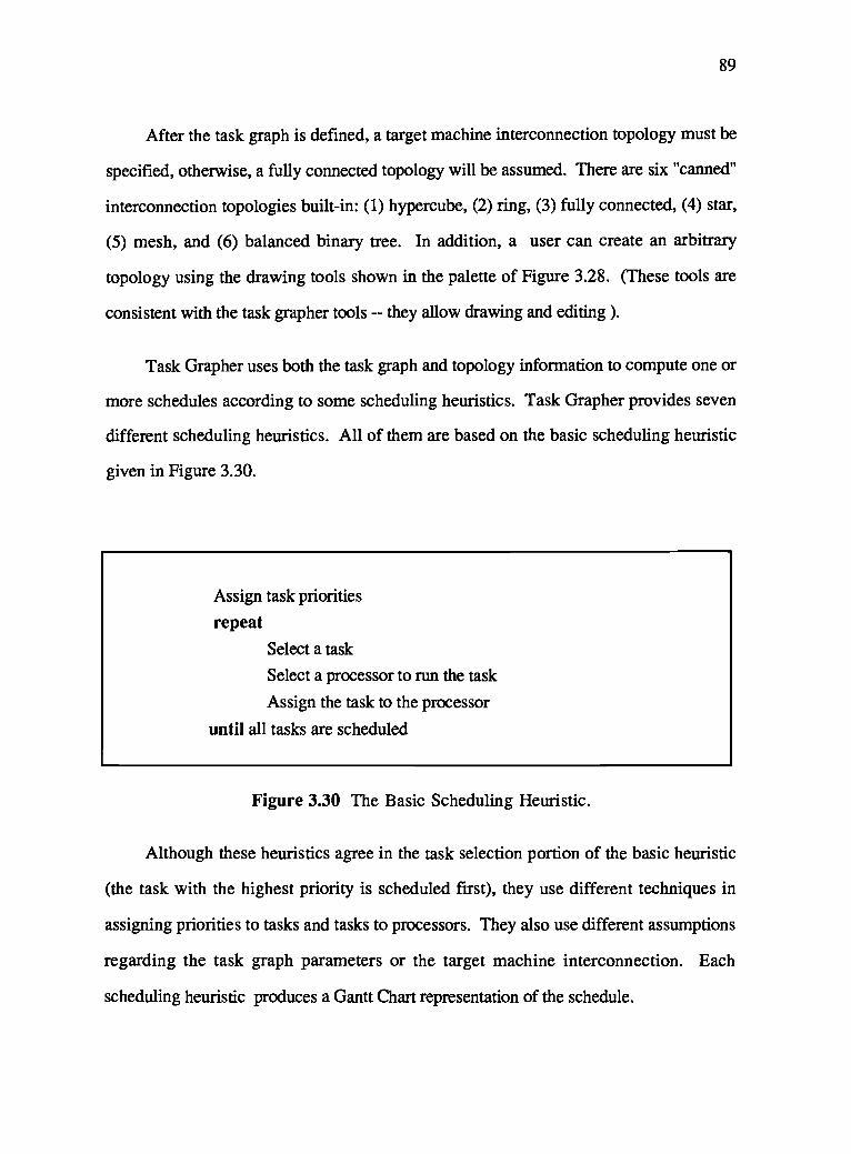
89

After the task graph is defined, a target machine interconnection topology must be

specified, otherwise, a fully connected topology will be assumed. There are six "canned"

interconnection topologies built-in: (1) hypercube, (2) ring, (3) fully connected, (4) star,

(5) mesh, and (6) balanced binary tree. In addition, a user can create an arbitrary

topology using the drawing tools shown in the palette of Figure 3.28. (These tools are

consistent with the task grapher tools -- they allow drawing and editing ).

Task Grapher uses both the task graph and topology information to compute one or

more schedules according to some scheduling heuristics. Task Grapher provides seven

different scheduling heuristics. All of them are based on the basic scheduling heuristic

given in Figure 3.30.

Assign task priorities

repeatSelect a task

Select a processor to run the task

Assign the task to the processor

until all tasks are scheduled

Figure 3.30 The Basic Scheduling Heuristic.

Although these heuristics agree in the task selection portion of the basic heuristic

(the task with the highest priority is scheduled first), they use different techniques in

assigning priorities to tasks and tasks to processors. They also use different assumptions

regarding the task graph parameters or the target machine interconnection. Each

scheduling heuristic produces a Gantt Chart representation of the schedule.

90

Method 1 (Hu Without Communication)

This method which is introduced by Hu [Hu61] assumes that there is no

communication delay. It uses a level number for setting task priorities which is the length

of the longest path from the task node to the ending node. Tasks are executed in highest-

level-first (HLF) order, then level-by-level. Only the execution times of tasks, and not

the communication delays, are counted in the longest path.

Method 2 (Hu With Communication)

This method is a modification of method 1 that considers communication [Krua87].

Task selection criterion remains the same as described in method 1. The communication

delay is included in computing the start time of a selected task when selecting a processor.

The processors containing the assigned node's immediate predecessors are considered

first in an attempt to reduce communication delay by placing message source and

destination tasks in the same processor.

Method 3 (Equal Node Size)

The method introduced by Yu [YuHo84] is used. This method assumes that tasks

have equal execution time and selects the best one of the processors which will be ready

within the next execution time unit. In this method, the average node size in the graph is

used as a substitute for all node sizes.

Method 4 (ISH)

Kruatrachue [Krua87] extended Hu's results by inserting a communication delay

between tasks, leading to the Insertion Scheduling Heuristic, ISH that tries to utilize the

idle time by inserting ready tasks into idle time slots. This added factor complicates the

scheduling problem, but offers a more realistic result. Furthermore, the communication

91

delay-time introduces a new problem, called the "max-min" problem, which concerns the

trade-off between maximum parallelism and minimum communication delay [Krua87].

In other words, the cost of message transmission is related to the degree to which parallel

processing takes place. Since the longest path reflects not only execution time, but also a

communication delay-time, the addition of processors may result in increased time for the

completion of all tasks. Frequently, this results in a system which is even slower than

sequential processing.

Duplication Scheduling Heuristics (DSH)

Kruatrachue [Krua87] proposed a second heuristic which uses duplication of tasks

to offset communication. The Duplication Scheduling Heuristic DSH is similar to ISH,

except that it solves the "max-min" problem by means of task duplication. This heuristic

is used in methods 5 and 6.

Method 5 (DSH-1 ... Duplication of One Preceding Task)

This heuristic is a DSH method which duplicates only immediate predecessors,

causing a communication delay, before each task is allocated. This lowers the time-

complexity of DSH, but may decrease the quality of the schedule.

Method 6 (DSH-2 ... Duplication of All Preceding Tasks)

This is a full DSH method which duplicates all of the ancestor tasks which

influence communication delays for each assigned task. The time complexity of this

heuristic is O( M4 ), where M is the number of tasks in the task graph.

Method 7 (MH)

This heuristic uses the mapping heuristic given in section 3.4.

92

3.7.3 Output From Task Grapher

The principle outputs from Task Grapher are the Gantt Chart and the Speed-up Line

Graph as described above. In addition, Task Grapher produces several useful displays

and measures of scheduling effectiveness. These displays and measures help parallel

program designer to get a clear picture of the performance of a parallel program

(represented by a task graph) when it runs on a certain target machine. Task Grapher

produces the following displays: 1) Gantt Chart Schedule, 2) Speed-up Line Graph, 3)

Critical Path In Task Graph, 4) Processor Utilization Chart, 5) Processor Efficiency

Chart, 6) Dynamic Activity Display.

We believe that the output of Task Grapher provides program designers with the

necessary information to find the best scheduling heuristic for a particular program on a

particular target machine. It also can help in tuning the task graph representing a parallel

program. For example, a program designer might need to explode a node into two or

more nodes if the load is not well balanced among the available processors or to implode

some nodes in order to reduce communication overhead. The minimum number of

processors to run a program with satisfactory performance can also be obtained.

Several interesting displays which have not been discussed are described below.

We use the following definitions:

m = number of processors

n = number of tasks

Time(m) = Execution time for m processors to execute in parallel

Comp(i) = Amount of time processor i spends doing computation.

93

Idle(i) = Amount of time processor i is idle.

S(m) = Speed-up due to m parallel processorsTime(1)

U(i) = Processor utilization(i)Comp(i)

Comp(i) + Idle(i) '1 < i 5- m.

E(m) = Average processor efficiency due to m parallel processorsS(m)

m

Processor Utilization Chart

A bar chart is displayed showing the percentage of total processor time performed

by each of the m processors. The parameter U(i) is displayed, 1 i 5. m. This chart can

be used to study processor load balance. Figure 3.31 shows a processor utilization bar

chart produced by Task Grapher.

Average Processor Efficiency Chart

Another bar chart is displayed showing the parameter E(m) where m varies from 1 to

an upper limit specified by the Task Graph user. As shown in Figure 3.32, the efficiency

chart can help to study the effect of using target machines with different number of

processors on the efficiency.

* File Edit Schedule Machine Analyze Layout

60

UT IL IZ AT ION

40

20

03 111

0 1 2 3 4 5

Processor Number

.14'; : :=I :*: :':::

94

Figure 3.31 Processor Utilization Chart of a Target Machine With Six Processors.

Produced by Task Grapher.

r a File Edit Schedule Machine finalyze Layout

95

Untitled

Efficiency %

100

90

80

70

60

50

40

30

20

10

0

1 2 3 4 5 6

Number of Processors

ice jM

Figure 3.32 Average Processor Efficiency Chart Produced by Task Grapher.

Dynamic Activity Display

Greater insight can be obtained by watching a parallel program execute, dynamically.

Task Grapher incorporates a design simulator which shows the dynamic behavior of the

parallel program design. This is done by animation of the topology screen.

Tasks are dynamically assigned to processors as execution of the parallel program is

simulated over time. The number of the node that is currently executing on each

processor is displayed in a box above each processor node. When the task terminates, it

is replaced by the next task to execute, or else the processor goes idle. Figure 3.33

shows a snap shot of the dynamic activity display.

r tt File Edit Search Project Run Debug Windows

96

-,

ii:iiif:;.:r illi:,.: :-i ir" hi '1

Figure 3.33 Dynamic Activity Display of a Task Graph on 6 Processors Forming a

Fully Connected Machine. At the Time of the Snap Shot Tasks 1, 2, 7, 10, 15, and 46

were Assigned to Processors 2, 0, 5, 3, 4, and 1 Respectively.

97

3.8 Summary

A new scheduling heuristic (MH) was introduced with the following characteristics:

1) inputs to the scheduler are a) an arbitrary labelled task graph representing a parallel

program with estimated node execution time, estimated message size, and b) a target

machine description which includes the transfer rate, initialization time, and

interconnection topology, 2) schedules are computed by an adapted highest-level-first

heuristic, and 3) contention is considered when making scheduling decisions.

The results for scheduling simulated task graphs on ring, star, mesh, hypercube,

and fully connected networks were introduced. On hypercubes these simulations suggest

that 1) communication delays should be considered in task selection when scheduling

communication intensive applications, 2) priority scheduling is insensitive to the

communication delays of computation intensive applications, 3) performance decreases

with the increase in the ratio between average communication and average task execution

time, 4) the effect of increasing the task graph average degree increases as the number of

processing elements increases, and 5) the average degree parameter is a good indicator of

the amount of communication in the task graph.

A tool for scheduling parallel programs called Task Grapher was introduced. It

implements a number of scheduling heuristics which have been proposed by the

literature. To our knowledge, Task Grapher is unique, and provides a tool for studying

the practicality and quality of these proposed heuristics. In addition, Task Grapher has

given us insight into the nature of task scheduling that no other tool provides.

Task Grapher was designed to be used iteratively to tune real applications [Judg89].

Because the accuracy of performance predictions made by Task Grapher depends on the

accuracy of the time estimates given to it, initial estimates of execution time, and message

98

passing time are merely guesses which must be improved upon by successive

approximation.

The animation feature of Task Grapher gives immediate feedback and insight into

the dynamic behavior of parallel programs. Idleness, congestion, and other measures of

"goodness" become vividly obvious after only a few minutes of using Task Grapher.

These observations do not always support intuition, and lead to a new understanding of

parallel programming.

Chapter 4

Loop Unrolling

4.1 Introduction

99

Scheduling is a computationally intensive problem [Car184, CoGr72, Ullm75]. But

static scheduling of task graphs that contain loops is even harder, especially when the

loop upper bound is not known before execution time. Loops in parallel programs have

been studied by many researchers in the areas of compiler optimization and mapping tasks

onto parallel computers [Wolf89, WuLe88, ZaSa88]. Work has been done on the

transformation and reduction of recurrences in sequential loops and partitioning such

loops into independent sequential loop components which could execute in parallel

[Padu80, PeGa87]. Wolfe [Wolf89] has studied several high level compiler loop

transformations, namely vectorization, concurrentization, loop fusion, and loop

interchange in order to speed up the execution of loops using parallel computers. The

Doacross technique [Cytr87], takes advantage of loop-carried dependences and provides

a unified framework to schedule sequential and parallel loops for both SIMD and MIMD

parallel machines. Although relatively efficient schedules can be obtained for sequential

loops using the Doacross scheduling technique, fine grained parallelism in such loops is

not exploited.To utilize fine-grained parallelism in a sequential loop, some compilers

unroll the loop body several times and compact the produced code by treating the unrolled

loop as an acyclic dependence graph. Zaky [ZaSa88] showed that when a relatively high

degree of hardware parallelism is available in the system, simple loop unrolling is not an

effective approach to extracting parallelism. He gave an algorithm that produces an

optimal synchronous schedule for an innermost sequential loop on an idealized parallel

processor system with an unbounded number of processors. Wu [Wu88] has also

100

introduced a load balancing technique called loop spreading that evenly distributes parallel

tasks on multiple processors without decrease in performance even when the size of the

input data is not a multiple of the number of processors.

Scheduling tasks contained in a loop on parallel computers can be achieved using

two different approaches: 1) tasks in the same iteration are assigned to the same

processor, and 2) tasks in the same iteration can be assigned to different processors.

Using the first approach, each iteration is assigned to a different processor unless there

are more loop iterations than processors. If the tasks in different iterations are completely

independent, no synchronization is needed. On the other hand if there are data passed

from one iteration to another, the processors need to be synchronized. Assigning all

tasks in one iteration to the same processor completely ignores any parallelism that might

occur within each iteration. Also, when data are passed from one iteration to another, the

synchronization delay might slow down the execution. The second approach does not

require that every task in the same iteration to be assigned to the same processor. The

results might be better if the tasks contained in a loop are independent so we can take

advantage of the parallelism exist among those tasks.

In this work we discuss a loop unrolling technique that might allow several

iterations of a set of loops as well as tasks within the same iteration to overlap in

execution in such a way that minimizes the loop execution time. We use local

neighborhood search and simulated annealing techniques to achieve near-optimal mapping

of a set of n nested loops that can possess potential for concurrent execution on an

arbitrary target machine. The significance of this work is that 1) loop unrolling is

combined with scheduling, and 2) target machine dependencies are considered.

This chapter is organized as follows. In section 4.2 we give a brief introduction

about data dependences and a representation of loop-independent and loop-carried

101

dependences [Wolf89] in loops. We then discuss loop unrolling in section 4.3. Section

4.4 introduces loops execution time computation. The optimization problem is introduced

in section 4.5. We give the formulation of the loop unrolling optimization problem in

section 4.6 and some examples are given in section 4.7. Finally, we give a summary in

section 4.8.

4.2 Dependence Among Tasks

A dependence between two tasks can be a data dependence or a control dependence.

A control dependence is a consequence of the flow of control in a program. For example,

the execution of a task in one path under an if test is contingent on the if test taking that

path. Thus, the task under control of the if is control dependent upon the if test. Data

dependency is a consequence of the flow of data in a program. A task that uses a variable

in an expression is data dependent upon the task which computes the value of the

variable. Dependence relations between tasks forming a program can be viewed as

precedence relations. If task Tw is control dependent or data dependent on task Tr then

execution of task Tv must precede execution of task Tw.

4.2.1 Dependence Between Tasks within loops

Data dependence can be further classified as loop-carried and loop-independent data

dependence. When some tasks are contained in n nested loops, we can refer to separate

instances of their execution using an iteration vector. A vector I = is

called an iteration vector if the loop body is executed in the period when the jth level loop

hisin the .t iteration, 15 j n. Simply, an iteration vector holds the values of the loop

control variables of the n nested loops. Using iteration vectors, we can define a

distance vector for each dependence between tasks. Suppose that v and w are two

tasks surrounded by n nested loops. If w during iteration /w is dependent on v during

iteration /v the distance vector for this dependence is Id = Iw - Iv. Task w is "loop-

102

carried" data dependent on task v iff /w * 11, (the distance vector elements are not all

zero). Otherwise the dependence is called "loop-independent" (the distance vector

elements are all zero). Elements of iteration and distance vectors are numbered from

outermost to innermost. Loops are also numbered from outermost to innermost and we

will refer to loops at different levels using those numbers. For example, the outermost

and innermost loops are at levels 1 and n, respectively.

We assume that loops are normalized to iterate from one to some upper bound in

steps of one. Non-normalized loops can be normalized through simple transformations

[Wolf89]. We also assume perfect (tightly) nested loops which means a set of tasks

enclosed in a set of nested loops. At least two ways of transforming imperfectly nested

loops into perfect ones have been developed: loop distribution [Wolf89], and the Non-

Basic-to-Basic-Loop transformation [AbuS78]. The last assumption we make is that all

distance vectors can have only positive values to guarantee acyclic loop-carried data

dependence.

Example 4.1

In the program given in Figure 4.1, we have a single loop (n = 1). Task T2(i) uses

a[i] which is computed in task T1(i) during the same iteration so T2 is "loop-

independent" data dependent on T1 and the distance vector = <0>. There is also "loop-

carried" data dependence between tasks T3 and T2 because T3(i) uses c[i -1] which is

computed in T2(i) in a previous iteration. So 1'3 is "loop-carried" data dependent on T2

and the distance vector = <1>.

103

for (i = 1; i 5. 10; i++)

{

T1(i); /* computes a[i] *1

T2(i); /* uses a[i] and computes c[i] */

T3(i); /* uses c[i-1] */

}

Figure 4.1 Three Tasks in Single Loop.

4.2.2 Dependency Matrix (DM)

We define a dependency ordered pair between two tasks w, during iteration

/w, and v, during iteration as as (Id ,D ) where Id is the distance vector Id= Iiv - Iv and

D is the message size (in bytes, for example) that w receives from v. Task w can have

more than one data dependency ordered pairs from task v. This multi-dependence

between v and w can be represented using a dependency set. The dependency set

between two tasks is the set of all dependency ordered pairs between those tasks. For

example, in the program given in Figure 4.1, we assume that each array element occupies

4 bytes. The dependency sets between T1 and T2, and T2 and T3 are { (<0 >,4) } and

{ (<1>,4) } , respectively.

Let V be the set of all the tasks that are surrounded by n nested loops (k = IVO.

Loop-carried and loop-independent data dependence among the tasks in V can be

represented using a kxk Dependency Matrix (DM). DM[i,j] represents the dependency

set from task, .1

v.J

to v.1

where v. ' 1v. E V. A (1) entry in DM[i,j] means that there is no

dependence from n to vi. We also define the task size array (TSA) as an array of

length k. TSA[i] represents the size of task vi.

104

We define the maximum distance vector for a matrix DM to be <m1, m2,...,

me>, where mi ?_ xi, xi is the ith component in a distance vector Id, Id is the first

component in an ordered pair p, p a set DM[i,j], 1 5 i 5 k, and 1 5 j 5 k. We also

define the upper bound vector for n nested loops to be <bi,b2,...,be>, where bi is

the upper bound of the loop at the ith level (notice that the outermost loop is at the first

level and the innermost loop is at the nth level). We assume that the upper bound vector

is unknown before execution time.

Example 4.2

Figure 4.2 shows an example of a DM that represents loop-carried and loop-

independent data dependence between tasks a and b that are enclosed in 2 nested loops.

It also shows the array TSA for tasks a and b. DM[1,1] = { (<1,0>,5),(<1,1>,10)}

means that an instance of task a during iteration <i1,i2>, for example, is data dependent

on instances of itself during iterations <ii-1,i2> and <i1-1,i2-1>, respectively and the

data sizes are 5 and 10 bytes respectively, DM[1,2] = CD means that there is no data

dependence from b to a, DM[2,1] = { (<0,0>,20)} means that b is data dependent on a

during the same iteration and the data size is 20 bytes (Notice that this is a loop-

independent data dependence), and finally DM[2,2] = { (<1,0>,12)} means that an

instance of task b during iteration <ji,j2>, for example, is data dependent on an instance

of itself during iteration <ji-1,j2> and the data size is 12 bytes. The maximum distance

vector for DM in Figure 2 is <1,1>. The size of tasks a and b are 7 and 9 respectively as

given in TSA.

105

4.3 Loop Unrolling

When a single loop, with upper bound b, is unrolled u times, u + 1 copies of the

body are replicated, the loop control variable is adjusted for each copy, and the step value

of the loop is multiplied by u + 1. For example, a loop unrolled one time should be

executed at least L li ] iterations.

Consider a set of n nested loops, with upper bound vector = <bi,b2,...,bn>, and

unrolling vector = <upu2,...,un>, that is the ith loop is unrolled ui times (loops aren

numbered from outermost to innermost). After unrolling, 11(ui+1) copies of the bodyi=1

are replicated, the loop control variables are adjusted for each copy, and the step value of

the ith loop is multiplied by ui+1.

nFor each v.

JE V in the pre-unrolling loop, there are 1-1(ui+1) tasks namely

i=1

lv.JY 'Y2 ..... Yn, (0 _ yi ui, 1 i n) in the post-unrolling loop.

For example, in Figure 4.3, the loop shown in (b) results from unrolling the loop

given in (a) once (u = <1>). Figure 4.4 shows another example when 2 nested loops are

used. Consider the nested loops given in (a), Figure (b) shows the loop resulting from

unrolling the innermost loop once (u = < 0,1>). Similarly Figure (c) shows the loop

resulting from unrolling the outermost loop once (u = <1,0>). Finally Figure (d) shows

the loop resulting from unrolling both loops once each (u = <1,1>). In the examples

given in Figures 4.3 and 4.4, the loop upper bounds are assumed to be multiple of two

for simplicity.

106

a b

a {(<1,0>,5) , (<1,1>,10)} c1

b {(<0,0>,20)} {(<1,0>,12)) b (9)

DM TSA

Figure 4.2 DM and TSA for Two Tasks a and b Enclosed in Two Nested Loops.

for (i = 1; i 5_ 2*ni; i++) for (i = 1; i 2*ni; i = i+2)

{ {

v Tl(i); v0 T1(i);

w 12(i); w° T2(i);

}v/ Tl(i +1);

w/ T2(i +1);

Figure 4.3 An Example for Unrolling a Single Loop Once (u = <1>).

107

for (i = 1; i 2*ni; i++) for (i = 1; i 2*ni; i = i++)

for (j = 1; j. 2*n2; j++) for (j = 1; j __ 2*n2; j = j+2)

{ {

v T(i,j); v00 T(i,j);

}v01 T(i,j+1);

(a)

for (i = 1; i 2*ni; i = i+2) for (i = 1; i 2*ni; i = i+2)

for (j = 1; j5. 2*n2; j++) for (j = 1; j 5. 2*n2; i = j+2)

{ {

v00 T(i,j); v00 T(i,j);

v10 T(i+1,j) 1,01 T(i,j+1);

}v10 T(i+1,j);

v11 T(i+1,j+1);

}

(c) (d)

Figure 4.4 (a) Original Loop, (b) Innermost Loop is Unrolled Once (u = <0,1>), (c)

Outermost Loop is Unrolled Once (u = <1,0>), and (d) Both Loops are Unrolled once

each (u = <1,1>).

108

Since loop-carried dependences may allow several iterations of a set of loops to

overlap in execution, loop unrolling can help to exploit the parallelism that might exist

among different iterations.

We give two examples that show how loop unrolling can help in minimizing the

loop execution time and in improving the performance. In both examples we assume that

the communication time between any two tasks running on the same processor is

negligible.We also assume that the processing speed and the transfer rate in the target

machine is always unity (this allows us to deal with the message size and the task size as

units of time).

Example 4.3

Consider the DM and the TSA given in Figure 4.5. Tasks a and b with task size =

15 as shown in the TSA are enclosed in a single loop (n = 1). DM[1,2] = { (<1>,10)}

means that an instance of task a during iteration <i>, for example, is data dependent on

an instance of task b during iteration <i-1> and the data size is 10 bytes, and DM[2,1]

={ (<1>,10) } means that an instance of task b during iteration <j>, for example, is data

dependent on an instance of task a during iteration <j -1> and the data size is 10 bytes.

Notice that there is no loop-independent data dependence between the two tasks which

means that within one iteration tasks a and b can run totally in parallel. Let's assume

(just for the sake of discussion) that the upper bound b of the loop is known and b = 4.

In the case when we have only one processor, tasks a and b run sequentially in any

order (we assume that task a executes first) and this process is repeated 4 times with total

execution time = 120 units of time as shown in Figure 4.6a.

Now suppose that we have two processors connected together and we are going to

exploit only the parallelism within each iteration and neglect the parallelism that might take

109

place if we unroll the loop. We run tasks a and b concurrently on processors pi and p2,

respectively so each iteration takes only 15 units of time. Since task a during iteration

<i> receives data from task b during iterations <i-1> and task b during iteration <j>

receives data from task a during iteration <j-1> and since tasks a and b are scheduled on

different processors, a new iteration has to wait for 10 units of time before starting

execution. Figure 4.6b shows that each iteration takes 15 units of time, however due to

the communication delay a new iteration can be initialized every 25 units of time and the 4

iterations take 90 units of time. If we unroll the body of the loop once we are able to

initialize a new iteration every 30 units of time without having to wait for any

communication and the total execution time is only 60 units of time as shown in Figure

4.7. By exploiting the parallelism without unrolling we get speedup =13 , however after

loop unrolling once speedup = 2 (which is the maximum theoretical speedup we can get

using two processors).

It is not always the case that we have zero communication delay between iterations

because it depends on the way we assign the tasks to the available processing elements.

a b

a clo { (<1>,10)} a (15)b ( ( (<1>,10)) clo b 15)

DM TSA

Figure 4.5 DM and TSA for Two Tasks a and b Enclosed in a Single Loop.

30

60

90

120

P1

a

b

a

b

a

b

a

b

Titeration 1 15

Titeration 2

+iteration 3

Titeration 4

±

25

40

50

65

75

90

P1 p2

a b

a b

a b

a b

iteration 1

delay

iteration 2

delay

iteration 3

delay

iteration 4

communication time

I:=3 execution time

(a) (b)

Figure 4.6 Gantt Charts Result From Scheduling Four Iterations of the Loop on One

and Two Processing Elements.

110

15

30

45

60

Figure 4.7 Gantt Chart Results From Scheduling Two Iterations of the Unrolled Loop

on Two Processing Elements

IA p2

a0

b0

b1

a1

a0

b0

b1

a1

iteration 1

iteration 2I

111

Example 4.4

In the case of nested loops, the performance might differ depending on which loop

is unrolled. Figure 4.8 shows the DM and the TSA for tasks a and b enclosed in 2

nested loops. DM[1,2] = { (<1,0>,5), (<0,1>,20)} means that an instance of task a

during iteration <i1,i2> (say) is data dependent on instances of task b during iterations

<i1-1,i2> and <i1,i2-1> and the data size is 5, 20 bytes respectively, and DM[2,1]

= { (<1,0>,5),(<0,1>,20)} } means that an instance of task b during iteration , say,

<j1,j2> is data dependent on an instance of task a during iterations <j1-1,j2> and <j i,j2-

1> and the data size is 5, 20 bytes respectively. Notice that there is no loop-independent

data dependence between the two tasks which means that within one iteration tasks a and

b can run totally in parallel. Figures 4.9a, b, c show the original loop, the loop after

unrolling the outermost loop once, and the loop after unrolling the innermost loop once.

The Gantt chart given in Figure 4.10a shows that when the outermost loop is

unrolled once, a new iteration has to wait 10 units of time because task a (b) during

iteration (i,j) receives data from task b (a) during iteration (i,j-1) and they are located on

different processors. That leads to 110 units of time total execution time. On the other

hand, when the innermost loop is unrolled once, no delay is needed and the total

execution time is 80 units of time as shown in Figure 4.10b.

a

b

a

cI)

( {(<1,0>,5),(<0,1>,20)}

b

{(<1,0>,5),(<0,1>,20)}

clo

a (10)b 10)

DM TSA

Figure 4.8 Two Tasks a and b Enclosed in Two Nested Loops Represented Using

DM and TSA.

For i = 1, 2

For j = 1,4

a; b;

(a)

For i = 1, 2, 2 For i = 1, 2

For j = 1,4

00 00 10 10a; b; a; b

For j = 1,4, 2

70 00 01 01a; b; a; b

(b) (c)

112

Figure 4.9 (a) Original Loop, (b) the Loop After Unrolling the Outermost Loop Once,

and (c) the Loop After Unrolling the Innermost Loop Once.

p1 p2 pl p2

10

20

30

40

50

60

70

80

90

100

110

i = 1, j = 1 10

20

delay

30

i=1,j= 2 40

50

delay

i= 1,j=3

delay

i=1,j= 4

60

70

80

b0000

a

01 01a b

00

b 00 a

01 01a b

00b00 a

01 01a b

00b00 a

01 01a b

i = 1, j = 1

i = 1, j = 3

i= 2,j= 1

i=2,j=3

= Communication= execution

(a) (b)

Figure 4.10 (a) The Schedule After Unrolling the Outermost Loop Once, and (b) the

Schedule After Unrolling the Innermost Loop Once.

113

4.4 Execution Time in Nested Loops

4.4.1 Definitions

Given a DM that represents data dependence among tasks enclosed in a set of n

nested loops with an upper bound vector b = <bi,b2,...,bn> and an unrolling vector u =

<ui,u2,...,un>. We define the following:

Lu: is the post-unrolling body which is enclosed in n nested loops when it is unrolled

according to unrolling vector u (we use L0 to refer to the original body without

unrolling).

tu,k: is the time to execute a loop at level k. Notice that tu,n+i is the time to execute

Lu only once, where Lu is the body of the innermost loop, and that tio is the time to

execute the outermost loop (the whole thing).

Xu jc: is the communication delay between any two consecutive iterations of a loop at

level k, where Lu is the body of the innermost loop. Notice that XII* = 0 when uk =

bk-1 because when we unroll a loop at the kth level bk -i times we generate all the

instances of that loop.

Gu = (V',E): is a directed acyclic data dependence graph that represents a loop body

Lu, where V' is the set of all tasks generated in Lu and E is the set of edges that

represent loop-independent and loop-carried data dependence generated from DM.

The graph Go represents L0 (notice that Go has only loop-independent data edges).

Figure 4.11 shows Gu that represents Lu, represented by DM and TSA given in

Figure 4.2, when u = <1,1>. The upper portion of each node contains the task title while

the lower portion contains the task size. The number next to an edge represents the

message size to be passed through that edge.

114

Figure 4.11 Gu That Represents Lu, Represented by DM and TSA Given in Figure

4.2, when u = <1,1>.

4.4.2 Execution Time Formulas

Given a DM that represents data dependence among tasks enclosed in a set of n

nested loops with an upper bound vector b = <b1,b2,...,bu> and an unrolling vector u =

<u1,u2,...,uu>. The time to execute the nested loop can be obtained as follows.

r bi 1 r bi 1 bitu,i 1 u+1 1 (tu,2 + Alo.) Av,1 (1 u+1 ' - u+1 ) °cu,2

(4.4.1)

Changing the unrolling vector (u) might change loop execution time. The best value

of the unrolling vector would be the one that gives the shortest loop execution time.

When the upper bound vector (b) is known before execution time, formula 4.4.1 can be

used to compute the execution time. Different values of the unrolling vector (u) can be

tried in order to find the shortest execution time. When the upper bound vector (b) is not

known, another formula that does not contain b is needed to compare the effect of using

different values of the unrolling vector.

Formula 4.4.1 can be bounded as:

b± 1 tt 15r u 1 1( 2 +u, u, X 1)u,

1

(4.4.2)

tu,1 can be approximated as:

bitu,1 (tu,2 Xu,i)

The time to execute a loop at level k can be approximated as follows.

k ukbku, (ru,k+14- Xtod, 1 k S n

115

(4.4.3)

(4.4.4)

Using formula 4.4.4, the time to execute the outermost loop can be obtained as

follows:

'C

1 b(u

2 (u ( ( (4.u 1 u

b+1 k +1 +19 1 _2 _ u X u,2) Xu,l)un+1 ,n+1 Xu,n)+ ) Xu,3)

(4.4.5)

n n-1 2b. bi bi b11-1 .1 (t u,n+14,u,n) +

111+Au,2 u 1+1 A11,1

111+i=1 i=1111-1 X1141-1+ i=1

(4.4.6)

(When <u1,u2,...,un> = <bi-1,b2-1,...,bn-1 >, Auk = 0, 1 S k n and tn1 = tu,n+1)

Since 1 uk < bk then ubkic+i ?. 1, 1 k n, j is bounded by:

n

( .0 + )u+1 ,n+1 u,1=1

i=1

(4.4.7)

Notice that when n = 1 (single loop) the two formulas 4.4.6 and 4.4.7 are the same

which means.

bi1 1 (t 2 + X 1)u, u + u, u,

1

(4.4.8)

116

Using the mapping technique (MH) given in chapter 3, we can get the time to run

the tasks represented by the acyclic graph Gu representing Lu on a certain target machine

(Cu,n+ 1)*

To get the communication delay between any two consecutive iterations of a loop at

level k (A,u,k, 1 k < n) without knowing the upper bound vector is impossible.

However we can always obtain the worst case communication delay by considering only

one iteration for all levels greater than k (surrounded by loop at level k). Having the

Gantt chart produced by MH, the worst case (Xiu,k, 1 k < n) can be obtained as the

maximum time that a task has to wait until it receives a message from a task scheduled in

some previous iteration.

117

4.5 Combinatorial Minimization

In this section we introduce the loop unrolling technique to answer the following

question: How many times should the loop be unrolled to speed up the loop execution

time? and how should the tasks forming the body of the loop be mapped onto a given

arbitrary target machine?

Our goal is to find the vector u = <ui ,u2,...,un> such that tu ,1 (the objective

function) as given in the previous section is minimized. Notice that finding the optimal

tu,1 is an example of combinatorial minimization. The space over which the function is

defined is n-dimensional discrete but very large space, so it cannot be explored

exhaustively.

One way of dealing with this optimization problem is to start with some initial

solution and go greedily for the quick nearby solution. That is, from the starting point,

we go immediately downhill as far as we can go. This approach leads to a local, but not

necessarily a global, minimum. An example of this technique is Local Neighborhood

Search [JGDo87].

Simulated annealing is a probabilistic modification of traditional neighborhood

search techniques [PFTV86]. Both approaches find a solution to a combinatorial

optimization problem by starting with some solution and making a series of modifications

to the solution. In neighborhood search algorithms, modifications which improve the

solution by some given cost criterion are accepted and others are rejected. The acceptance

criterion in simulated annealing is more complex. All modifications which lead to a better

solution are accepted. All modifications which result in a poorer solution (higher cost)AE

are accepted with probability exp(- .7-) where AE is the difference between the costs of

the solutions before and after the update, and T is a parameter known as temperature.

118

Over time, the parameter T is slowly reduced, causing a reduction in the probability that a

modification which results in a poorer solution will be accepted. The simulated annealing

technique usually corrects a major flaw of neighborhood search technique the tendency

to get stuck in local minima in the solution space. For practical purposes, it has

effectively "solved" the famous traveling salesman problem of finding the shortest

cyclical itinerary for a traveling salesman who must visit each of N cities in turn. The

method has also been used successfully for designing complex integrated circuits: The

arrangement of several hundred thousand circuit elements on a tiny silicon substance is

optimized so as to minimize interference among their connecting wires. To make use of

the simulated annealing algorithm one must provide the following elements:

1. Configuration: A description of possible system configurations.

2. Update: A generator of random changes in the configuration; these changes are the

"options" presented to the system.

3. Objective Function: An objective function E (analog of energy) whose

minimization is the goal of the procedure.

4. Schedule: A control parameter T (analog of temperature) and an annealing

schedule which tells how it is lowered from high to low values, e.g., after how

many random changes in configuration is each downward step in T taken, and

how large is the step.

119

4.6 Loop Unrolling Problem Formulation

The loop unrolling optimization problem can be formalized as follows:

1. Configuration. A configuration is a vector u = <u1,u2,...,un>, where ui > 0; 1 5 i

< n.

2. Update. The update consists of two types: a) An i is chosen randomly in the range

[1,n] then ui is changed randomly; or b) some ui's (chosen randomly) are

changed randomly, 1 5 i 5 n.

3. Objective Function. The execution time as given in 4.4.7 is our objective function.

However since the upper bound vector b is usually not given before run time andn

since IT, does not change during the optimization search then the objectivei=1

function can be given as:

n1

nE = (

flui+1 i tun+1+i=1 A'iu,i1,i =1

) (4.4.9)

4. Schedule. The local neighborhood search method keeps trying until some

terminating condition happens. In the simulated annealing solution we choose a

starting value for the temperature parameter T greater than the largest AE. We

proceed downward in multiplicative steps each amounting to some decrease in T.

We hold each new value of T constant for some number of changes in the

unrolling vector, or for some number of successful moves, whichever comes

first. When effort to reduce E further becomes sufficiently discouraging, we

stop.

The problem now is how to choose the initial value of u. It can be noticed that the

maximum distance vector defined in section 4.2.2 is the minimum unrolling vector that

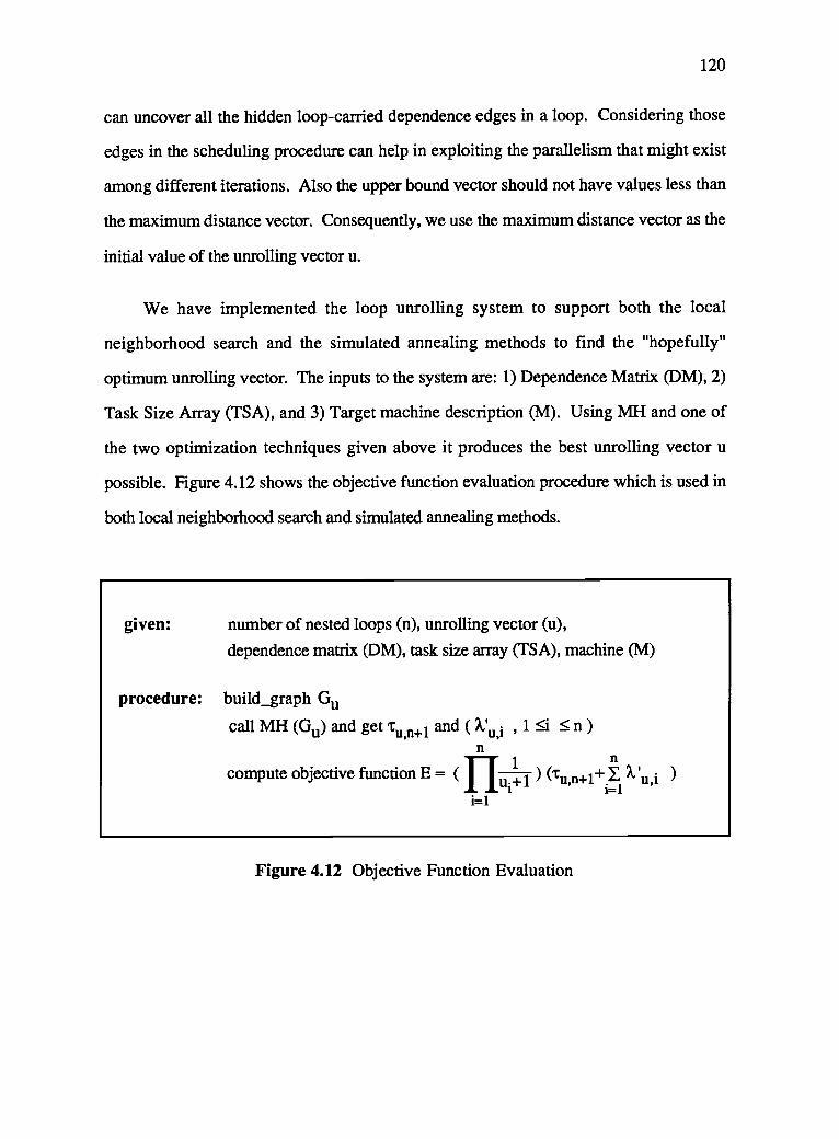
120

can uncover all the hidden loop-carried dependence edges in a loop. Considering those

edges in the scheduling procedure can help in exploiting the parallelism that might exist

among different iterations. Also the upper bound vector should not have values less than

the maximum distance vector. Consequently, we use the maximum distance vector as the

initial value of the unrolling vector u.

We have implemented the loop unrolling system to support both the local

neighborhood search and the simulated annealing methods to find the "hopefully"

optimum unrolling vector. The inputs to the system are: 1) Dependence Matrix (DM), 2)

Task Size Array (TSA), and 3) Target machine description (M). Using MH and one of

the two optimization techniques given above it produces the best unrolling vector u

possible. Figure 4.12 shows the objective function evaluation procedure which is used in

both local neighborhood search and simulated annealing methods.

given: number of nested loops (n), unrolling vector (u),

dependence matrix (DM), task size array (TSA), machine (M)

procedure: build graph Gu

call MH (Gu) and get tu,n+i and ( X'u,i , 1 5. n )

nill

)n

compute objective function E = ( ui+1 / tu,n+1+L x iu,ii=1

)

Figure 4.12 Objective Function Evaluation

121

4.7 Examples

In this section we study the performance of the local neighborhood search and the

simulated annealing methods in loop unrolling through examples. We introduce three

cases: 1) single loop, 2) two nested loops, and 3) three nested loops. We schedule all

three cases on a hypercube with four processing elements. In each case information

about the unrolling vector, the value of the objective function, number of nodes and edges

in the post-unrolling loops, and the average degree (number of edges ) in the post-number of nodes

unrolling loops are given in tabular forms. Also we give some curves that show the

change in the objective function with each move in the unrolling space.

In both methods we start with the maximum distance vector as initial unrolling

vector. Also the search space is restricted using some maximum values for the elements

of the unrolling vector. The local neighborhood search method keeps trying until some

terminating condition happens (in these examples we restricted the number of tries to

some number depending on the size of the search space). In the simulated annealing

solution we choose a starting value for the temperature parameter T greater than the

largest AE ( some random runs were made to find the range of AE). We proceed

downward in multiplicative steps each amounting to some decrease in T. We hold each

new value of T constant for some number of changes in the unrolling vector, or for some

number of successful moves, whichever comes first. When effort to reduce E further

becomes sufficiently discouraging, we stop.

4.7.1 Case 1: Single Loop (n = 1)

Figure 4.13 shows the DM and the TSA matrices for four tasks. It can be noticed

that there is no loop-independent data dependence edges which means that the four tasks

122

are completely independent within the same iteration. However, loop-carried data

dependence edges are shown in DM.

Since the four tasks are surrounded by a single loop, the search space is only one

dimension and exhaustive search can be applied to show the behavior of the objective

function (E) over the search space. Table 4.1 shows the move number, the unrolling

vector (the unrolling vector is just one element-- n = 1), the value of the objective function

(E), and number of nodes, number of edges, and the degree in the post-unrolling loop.

Figure 4.14 shows the change in the objective function (E), when unrolling

increases in steps of one. It can be noticed that the E changes up and down in a way that

increases the chance of being stuck in a local minimum. We thought that simulated

annealing would be the solution to this problem, however we tried both methods.

Table 4.2 and Figure 4.15 show the results of applying the local neighborhood

search. We restricted the number of tries to 20. This method made only three successful

moves out of 20 tries and the answer was best u = <12> with E = 6.7610.

Table 4.3 shows the simulated annealing solution. We proceeded downward in

multiplicative steps each amounting to a 20 percent decrease in T. We held each new

value of T constant for 8 changes in the unrolling vector or for 4 successful moves. We

also restricted the number of tries to 16. Simulated annealing made 9 successful moves

and the answer was best u = <12> with E = 6.7610. Figure 4.16 shows the change in E

with each successful move.

Of course it is meaningless to use either methods in this particular example as given

above because the exhaustive search can search the whole space in the same number of

tries. However we used that example with that restricted search space just to show the

difference between the two methods. And as shown from Tables 4.2 and 4.3, the two

123

methods found the same answer which happened to be the minimum in that restricted

search space.

1 2 3 411 { (<4>,8)} { (<1>,3),(<4>,20) } (<4>,9),(<3>,7),(<2>,8) } (<3>,1)}

2 {(<4>,14),(<1>,2)) { (<3>,4)} { ( <3 >,17),(<4 >,3) } (130

3 {(<3>,11)} {(<2>,20)} {(<3>,6)} CD

4\ {(<1>,4)} {(<3>,16),(<2>,13)} {(<2>,11)} {(<2>,10)} j

DM

1 9\2 2

3 13

4 4)TSA

Figure 4.13 DM and TSA for Four Tasks (1, 2, 3,and 4) Enclosed in a Single Loop.

movenumber

u1 Enumber

ofnodes

numberof

edgesdegree

1 4 8.4565 20 46 2.3002 5 10.3300 24 66 2.7503 6 10.4288 28 86 3.0714 7 9.3737 32 106 3.3125 8 8.7700 36 126 3.5006 9 8.9364 40 146 3.6507 10 7.2772 44 166 3.7738 11 8.2577 48 186 3.8759 12 6.7610 52 206 3.96210 13 7.4212 56 226 4.03611 14 6.9300 60 246 4.10012 15 8.3901 64 266 4.15613 16 7.9426 68 286 4.20614 17 7.6643 72 306 4.25015 18 6.9424 76 326 4.28916 19 7.5321 80 346 4.32517 20 7.4706 84 366 4.35718 21 7.1389 88 386 4.386

Table 4.1 Exhaustive Search (n = 1)

0 10

Move Number

20

124

Figure 4.14 The Change in E when the Loop is Unrolled From 4 to 21 Exhaustively

(n=1)

125

movenumber

u1 Enumber

ofnodes

numberof

edgesdegree

1 4 8.4565 20 46 2.3002 10 7.2772 44 166 3.7733 12 6.7610 52 206 3.962

E

Table 4.2 Local Neighborhood Search (n = 1)

9

8

7

60 1 2 3 4

Figure 4.15 Three Successful Moves in Local Neighborhood Search (n=1)

126

movenumber

u1 Enumber

ofnodes

numberof

edgesdegree

1 4 8.4565 20 46 2.3002 10 7.2772 44 166 3.7733 11 8.2577 48 186 3.8754 10 7.2772 44 166 3.7735 21 7.1389 88 386 4.3866 18 6.9424 76 326 4.2897 12 6.7610 52 206 3.9628 21 7.1389 88 386 4.3869 12 6.7610 52 206 3.962

E

Table 4.3 Simulated Annealing Solution (n = 1)

9

8

7 \A,0 2 4 6

Move Number

8 10

Figure 4.16 Nine Successful Moves in Simulated Annealing (n = 1)

127

4.7.2 Case 2: Two Nested Loops (n = 2)

In this example, as shown in figure 4,17, three tasks are surrounded by two nested

loops and the size of the three tasks are 11, 3, and 16 respectively. We restricted number

of tries to 40 and restricted the search space to 400 points by using maximum value = 21

for the two elements of the unrolling vector.

Table 4.4 shows the local neighborhood search solution and the answer was best u

= < 19, 18> with E = 7.5921 and number of nodes and edges = 1140, 5179 respectively.

Figure 4.18 shows that this method made only 5 successful moves out of 40.

The simulated annealing solution is given in Table 4.5 and the answer was the best

u = < 4, 11> with E = 8.3833 and number of nodes and edges = 180, 704 respectively.

Here simulated annealing performed worse than local neighborhood search, however the

post-unrolled graph is smaller than that of the other method.

Figure 4.18 shows that simulated annealing made 11 successful moves and missed

two good moves-- u = <16, 19> with E = 7.6352 and u = <15,11> with E = 7.6770.

1

2

3

1

(<0,2 >,3) }

{ (<2,1>,12)(<1,0>,9 ) )

{ (<0,1>,12)(<1,2>,7 )(<0,2>,7 )}

2

(1)

cro

{(<1,0>,10)(<0,2>,8 ))

3{(<0,1>,6 )(<2,2>,20)(<1,0>,8 ) )

{ (<1,1>,14)(<0,2>,12)(<0,1>,17)(<1,0 >,13)}

1

2 3

3 16

DM TSA

Figure 4.17 DM and TSA for Three Tasks (1, 2,and 3) Enclosed in Two Nested

Loops.

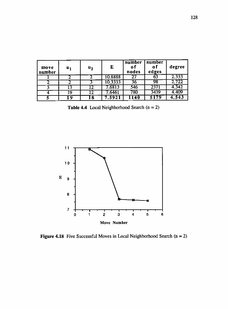
128

movenumber

ui u2 Enumber

ofnodes

numberof

edgesdegree

1 2 2 10.8888 27 63 2.3332 2 3 10.3333 36 98 2.7223 13 12 7.6813 546 2371 4.3424 19 12 7.6461 780 3439 4.4095 19 18 7.5921 1140 5179 4.543


0 2 3

Move Number

4 5 6

Figure 4.18 Five Successful Moves in Local Neighborhood Search (n = 2)

129

movenumber

u1 u2 Enumber

ofnodes

numberof

edgesdegree

1 2 2 10.8888 27 63 2.3332 2 3 10.3333 36 98 2.7223 13 3 8.2678 168 571 3.3994 3 19 8.5500 240 941 3.9215 16 19 7.6352 1020 4620 4.5296 6 19 7.8928 420 1790 4.2627 4 7 8.6500 120 444 3.7008 4 13 8.2285 210 834 3.9719 4 11 8.3833 180 704 3.91110 15 11 7.6770 576 2497 4.33511 4 11 8.3833 180 704 3.911


11

E 9

8

70 2

1 - 1 1

4 6 8 10

Move Number

12

Figure 4.19 Eleven Successful Moves in Simulated Annealing (n = 2)

130

4.7.3 Case 3: Three Nested Loops (n = 3)

Figure 4.20 shows DM and TSA for three tasks surrounded by three nested loops.

The sizes of the three tasks are 9, 3, and 6 respectively. In this example we restricted

number of tries to 40 and restricted the search space to 1000 points by using maximum

value = 11 for the three elements of the unrolling vector.

Table 4.6 shows the local neighborhood search solution and the answer was best u

= < 8,7,8> with E = 3.5216 and number of nodes and edges = 1944 and 6246

respectively. Figure 4.21 shows that this method made only 6 successful methods out of

40.

The simulated annealing solution is given in Table 4.7 and the best u = < 7,7,8>

with E = 3.6770 and number of nodes and edges = 1728 and 5492 respectively. Figure

4.22 shows that simulated annealing made 9 successful moves in the search.

1

I2 3

1 {(<0,2,0>,28 ) } (I) {(<0,0,1>,55 )(<2,2,0>,198)(<1,0,0>,74 ) )

2 { (<2,0,0>,116)4131

{(<0,1,0>,167)(<1,0,0>,81 )} (<1,0,0>,130))

3 {(<1,0,0>,120) {(<0,2,0>,73 ) ) cI)(<0,1,2>,65 )(<0,0,2>,68 ) ) /

1

2 3

3 6

DM TSA

Figure 4.20 DM and TSA for Three Tasks (1, 2, and 3) Enclosed in Three Nested

Loops.

131

movenumber

u1 u2 u3 Enumber

o fnodes

numbero f

edgesdegree

1 2 2 2 17.8148 81 153 1.8892 2 4 5 9.0000 270 651 2.4113 2 7 8 5.9120 648 1722 2.6574 2 6 8 5.6031 567 1485 2.6195 8 6 8 3.8342 1701 5391 3.1696 8 7 8 3.5216 1944 6246 3.213

E


00 1

. I - I - I

2 3 4

Move Number

5 6 7

Figure 4.21 Six Successful Moves in Local Neighborhood Search (n = 3)

132

movenumber

u1 u2 u3 Enumber

ofnodes

numberof

edgesdegree

1 2 2 2 17.8148 81 153 1.8892 2 8 2 11.2592 243 567 2.3333 7 2 8 6.7500 648 1732 2.6734 2 4 5 9.0000 270 651 2.4115 2 8 5 7.3271 486 1263 2.5996 7 8 7 3.9184 1728 5512 3.1907 7 8 6 4.1726 1512 4780 3.1618 7 8 8 3.6049 1944 6244 3.2129 7 7 8 3.6770 1728 5492 3.178


20

E 1 0 -

00 2 4

Move Number

8 10

Figure 4.22 Nine Successful Moves in Simulated Annealing (n = 3).

133

4.8 Summary

In this chapter we discussed scheduling unrolled loops onto arbitrary target

machines in a way that minimizes the completion time. We used local neighborhood

search and simulated annealing methods to find: 1) the best unrolling vector for a

particular set of tasks when they run on a particular target machine and 2) the Gantt chart

that indicates the allocation and the order of the tasks in the post-unrolled loop on the

available processing elements. We showed three simple examples for a single loop, two

nested loops, and three nested loops to show the performance of the two methods in each

case.

Another 20 random examples ranging from a single loop to four nested loops were

generated and were scheduled on a hypercube of dimension 2. In comparison with the

local neighborhood search, the performance of the simulated annealing method was either

much better or much worse than the performance of the local neighborhood search

method. The simulated annealing algorithm can be tuned by varying some parameters in

the algorithm such as starting temperature, temperature reduction policy, and exit

condition. Also the local neighborhood search method can be tuned by varying the exit

condition.

Since the two algorithms can be tuned through a set of parameters and since the

performance of the two methods differs from one task graph (represented using DM and

TSA) to another and from one target machine to another, we implemented both methods

in our tool.

It is recommended that the user tries both methods. By tuning the set of parameters

associated with each algorithm, a near optimal solution can be reached. We believe that

134

finding the best unrolling vector and the best schedule should be achieved through

iterative interaction between parallel program designers and the loop unrolling tool.

If the upper bound vector is known when the schedule is generated a complete

unrolling might be done to generate an acyclic graph to schedule. If the nested loops are

too large to unroll completely, then the exact formula for the time to execute the outermost

loop (tu,i) should be used as the objective function and some "reasonable" unrolling

vector can be obtained using the the local neighborhood search or the simulated annealing

techniques in a restricted search space.

If the upper bound vector is not known when the schedule is generated but is

known before the loop begins execution, then some maximum values for the elements in

the unrolling vector should be given by the user. These values might differ from one

application to another.

Having the unrolling vector, three different cases should be considered in the

program: 1) if the number of loop iterations is greater than and multiple of the unrolling

value, then no more iterations need to be executed after the unrolled loop, 2) if the

number of loop iterations is greater than and not multiple of the unrolling value, then the

tasks in the remaining iterations can still be assigned to the same processing elements they

were assigned to in the generated schedule, and 3) if the number of loop iterations is less

than the unrolling value, then the tasks in all iterations are assigned to the same

processing elements they were assigned to in the generated schedule.

Chapter 5

Conclusions and Future Work

5.1 Conclusions

135

We presented a graphical design language for parallel programming. ELGDF

allows the expression of the common structures in parallel programs easily and

compactly. ELGDF provides a vehicle for studying parallel programs.

A graphical design editor called Parallax is provided as a user friendly tool for

expressing parallel program designs in ELGDF. It helps as a way to capture parallel

program designs for the purpose of analysis. Parallax produces design files that contain

information needed by different tools in the PPSE [Lewi89].

More work can be done in ELGDF to make its syntax suitable for other parallel

programming paradigms such as data parallel programming.

A new scheduling heuristic (MH) was introduced that considers most of the

critically important features needed to model modern parallel processor systems: 1) tasks

may have different execution times, 2) communication links between tasks may consume

a variable amount of communication time, 3) communication links may be themselves

shared, thus giving rise to contention for the links, 4) the network topology may

influence the schedule due to multiple-hop links.

Insertion Scheduling and Duplication Scheduling heuristics [Krua87] that assume

fully connected target machines can use MH to produce more realistic schedules

considering target machine topology and the possibility of contention in the

communication links.

136

The results for scheduling simulated task graphs on hypercubes suggest that 1)

communication delays should be considered in task selection when scheduling

communication intensive applications, 2) priority scheduling is insensitive to the

communication delays of computation intensive applications, 3) performance is inversely

proportional to the ratio between average communication and average task execution time,

4) the effect of increasing the task graph average degree increases as the number of

processing elements increases, and 5) the average degree parameter is a good indicator of

the amount of communication in the task graph.

Task Grapher implements a number of scheduling algorithms which have been

proposed by the literature as well as MH. To our knowledge, Task Grapher is unique,

and provides a tool for studying the practicality and quality of these proposed algorithms.

In addition, Task Grapher has given us insight into the nature of task scheduling that no

other tool provides.

Task Grapher was designed to be used iteratively to tune real applications. Because

the accuracy of performance predictions made by Task Grapher depends on the accuracy

of the time estimates given to it, initial estimates of execution time, and message passing

time are merely guesses which must be improved upon by successive approximation.

After an initial schedule is computed, the parallel program is executed on a real

processor to obtain accurate estimates of task execution time and communication delay

time. These numbers are then fed back into Task Grapher to obtain an improved

schedule.

A loop unrolling technique was introduced to schedule nested loops onto arbitrary

target machines in a way that minimizes the completion time. We used local

neighborhood search and simulated annealing methods to find: 1) the best unrolling

137

vector, and 2) Gantt chart that indicates the allocation and the order of the tasks in the

post-unrolled loop on the available processing elements.

It is recommended that the user tries both methods and by tuning the set of

parameters associated with each algorithm a near optimal solution can be reached. We

believe that finding the best unrolling vector and the best schedule should be achieved

through iterative interaction between parallel program designers and the loop unrolling

tool.

If the upper bound vector is known when the schedule is generated a complete

unrolling might be done to generate an acyclic graph to schedule. If the nested loops are

too large to unroll completely, then the exact formula for the time to execute the outermost

loop should be used as the objective function and some "reasonable" unrolling vector can

be obtained using the the local neighborhood search or the simulated annealing techniques

in a restricted search space.

If the upper bound vector is not known when the schedule is generated but is

known before the loop begins execution, then some maximum values for the elements in

the unrolling vector should be given by the user. These values might differ from one

application to another.

5.2 Future Work

The following work is worthy of future research efforts:

1) Extending ELGDF to handle data partitioning paradigm.

2) Scheduling input-dependent task graphs (section 5.3 contains some thought

about scheduling branches statically).

138

3) How to characterize parallel algorithms as task graphs, and how to quantify the

performance that can be expected from certain kinds of task graphs running on

specific network topologies.

4) Given a program task graph, how to find the right machine size to achieve the

best performance (for example, the size of a subcube in a bigger hypercube).

5) Conducting large experiments to thoroughly assess MH.

6) A software tool for loop unrolling technique. The tool must include the

following:

- Graphical user interface.

Graphical notations for loop-carried dependency.

- A tool for transforming data dependence to the DM form.

- A tool for converting non-perfect loops to perfect ones.

- A tool for displaying the unrolled loop.

- Performance displays.

5.3 Thoughts about Scheduling Task Graphs with Branches

In this section we give some suggestions for solving the problem of scheduling

task graphs that contain branches. The major problem in having branches in task graphs

is simply the non-determinism because the direction of a branch may be unknown until

the program is midway in execution. So we overcome this problem by proposing a

probabilistic task graph to represent a parallel program. The probabilities used in the

139

proposed task graph model can be obtained by running the program different times for

different sets of input. Probabilistic models were used in [ChAb81, Fish81, Tows86].

Starting with the probabilistic task graph we suggest three different deterministic

task graphs we can easily obtain through simple transformation namely 1) Expected Task

Graph (ETG), 2) Most Likely Task Graph (MTG), and 3) Random Task Graph (RTG).

Any of these deterministic task graphs can be scheduled onto arbitrary target machines

using the MH algorithm given in chapter 3 of this thesis.

We first give the proposed program model that distinguishes between data and

control dependence in parallel programs in section 5.3.1. In section 5.3.2 we present the

three deterministic task graphs. Finally we give an example in section 5.3.3.

5.3.1 Probabilistic Program Model

A parallel program consists of M separate cooperating and communicating modules

called tasks. Its behavior is represented by a control and a data models. These models

are represented by acyclic directed graphs called Branch Activation Graph BAG =

(T,Ec) and Data Dependency Graph DDG = (T,Ed), where T is a set of M vertices

representing the program modules (tasks), Ec is a set of branch edges, and Ed is a set of

data edges.

A directed branch edge (Ti,Ti) between two tasks Ti and Ti exists if there is an execution

instance of the program such that the execution of Ti follows the execution of Ti. A data

edge (Ti,Ti) reflects data flow between Ti and Ti and Ti cannot start execution until it

receives some data from Ti after its completion.

Associated with each branch edge (Ti,Tj) is the probability P(Ti,Tj) that task Ti will be

executed immediately after Ti, with each data edge (Ti,Ti) is the data size D(Ti,Ti), and

140

with each task Ti are the number of instructions to be executed INS(Ti) and the

probability that the task will be executed j.t(Ti).

Let IMS = {v1, v2, ..., vm} is the set of all immediate successors of vertex u in

BAG. The following rule holds: E P(u,vi) = 1.i=1

5.3.2 Deterministic Task Graphs

5.3.2.1 Expected Task Graph

The expected task graph ETG = (T,Ed) considers all the possible paths in the

program. T and Ed are the sets of tasks and data edges, respectively as described in the

data model. Associated with each data edge (Ti,T.i) is the expected data size

D_exp(Ti,Ti), and with each task Ti is the expected number of instructions to be executed

INS_exp(Ti).

To calculate the new parameters D_exp(*) and INS_exp(*) we need first to calculate

the probability that each task (Ti) is executed p,(Ti).

Let u E T be any node (task) and IMP = (v1, v2, vm) be the set of all

immediate predecessor of u in BAG.

If IMP is empty (u is a source node)

then 11(u) = 1.

else

1.1(u) = P(vi,u)*R(vi).

i=1

Now the parameters D_exp(*) and INS_exp(*) are calculated as follows.

Let u e T, then INS_exp(u) = igurINS(u).Let (u,v) E Ed, then D_exp(u,v) = g(v)*D(u,v).

141

5.3.2.2 Most Likely Task Graph

The most likely task graph MTG = (T_s,Ed_s) gives the tasks and their data

dependency in the most likely path the program would take during execution. T_s is

subset of T and Ed_s is subset of Ed, where DDG = (T,Ed).

A node u E T_s iff any of the following is true in BAG.

u is a source node.

- there exist a node v and v e T_s and P(v,u) P(v,x) for all x such that x E

IMS, where IMS is the set of all immediate successors of v.

An edge (u,v) E Ed_s iff u, v E T_s and (u,v) E Ed.The parameters INS and D

are the same as given in the data model.

5.3.2.3 Random Task Graph

The random task graph RTG = (T_s,Ed_s) gives a random execution path of the

program. T_s is subset of T and Ed_s is subset of Ed, where DDG = (T,Ed).

A node u E T_s iff any of the following is true in BAG.

- u is a source node.

- there exist a node v and v T_s and u is randomly selected from the set of all

immediate successors of node v.

An edge (u,v) E Ed_s iff u, v E T_s and (u,v) E Ed.The parameters INS and D

are the same as given in the data model.

142

5.3.3 Example

Figures 5.1 and 5.2 show an example of a parallel program represented by a Data

Dependency Graph (DDG) and a Branch Activation Graph (BAG) consisting of 8 nodes

(M = 8), where each node represents a task.

In DDG, the number shown in the upper portion of each node is the node number,

the number in the lower portion of a node i represents the parameter INS(i), and the

number next to an edge (i,j) represents the parameter D(i,j). For example INS(1) = 10,

D(4,7) = 10.

IN BAG, the number shown inside each node is the node number and the number

next to an edge (i,j) represents the probability P(i,j). For example P(1,3) = 0.8.

Figure 5.3 shows the expected task graph (ETG). The number shown in the upper

portion of each node is the node number, the number in the lower portion of a node i

represents the parameter INS_exp(i), and the number next to an edge (i,j) represents the

parameter D_exp(ij). The number next to a node i represents the probability 1.1,(i). For

example INS_exp(5) = 2, p.(5) = 0.2, and D_exp(1,5) = 2.

Figures 5.4, 5.5 show MTG and RTG, respectively. The number shown in the

upper portion of each node is the node number, the number in the lower portion of a node

i represents the parameter INS(i), and the number next to an edge (i,j) represents the

parameter D(i,j).

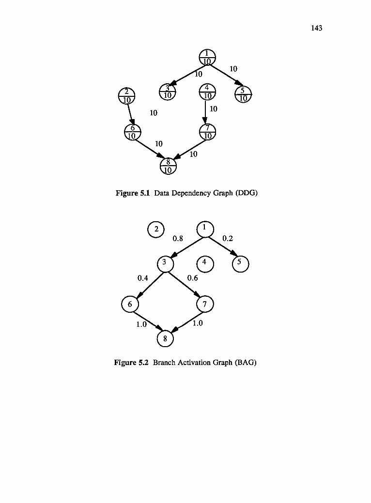
143

Figure 5.1 Data Dependency Graph (DDG)

Figure 5.2 Branch Activation Graph (BAG)

144

Figure 5.3 Expected Task Graph (ETG)

0.2

Figure 5.4 Most Likely Task Graph (MTG)

144a

Figure 5.5 Random Task Graph (RTG)

145

Bibliography

[AbuS78] W. Abu-Sufah, "Improving the Performance of Virtual MemoryComputers," Ph.D. Thesis, Dept. of Comp. Sci., Univ. of Ill. at Urbana-

Champaign, 1978.

[ACDi74] T. Adam, K. Chandy, and J. Dickson, " A Comparison of list Schedulers

for Parallel Processing Systems," Comm. ACM, vol. 17, pp. 685-690,

December 1974.

[Acke82] W. Ackerman, "Data flow languages," IEEE Computer, pp. 15-25,

February 1982.

[AdBr86] A. Adiga and J. Browne, "A graph model for parallel computationsexpressed in the computation structures language," proceedings of ICPP,

1986.

[AIKe82] J. Allen and K. Kennedy, " PFC: A program to convert Fortran to Parallel

Form," proc. of the IBM conference on parallel Computers and Scientific

Computations, 1982.

[A1Ke85] J. Allen, and K. Kennedy, " A Parallel Programming Environment,"

IEEE Software, pp. 21-29, July 1985.

[Babb84] R. Babb, "parallel processing with large-grain data flow techniques,"

IEEE Computer, pp. 55-61, July 1984.

[BaDi87] R. Babb and D. DiNucci, "Design and implementation of parallelprograms with large-grain data flow," in Characteristics of parallelalgorithms, Cambridge, MA: MIT Press, pp. 335-349, 1987.

[BASo89] J. Browne, M. Azam, and S. Sobek, "CODE: A Unified Approach toParallel Programming," IEEE Software, pp. 10-18, July 1989.

146

[Bokh8la] S. Bokhari, " A Shortest Tree Algorithm for Optimal Assignments Across

Space and Time in Distributed Processor System," IEEE Transaction on

Software Engineering, vol. SE-7, no. 6, November 1981.

[Bokh8lb] S. Bokhari, "On the Mapping Problem," IEEE Transactions onComputers, C-30, 3, pp 207-214, 1981.

[CaKu88] T. Casavant, and J. Kuhl, " A Taxonomy of Scheduling in GeneralPurpose Distributed Computing Systems," IEEE Transaction on Software

Engineering, vol. SE-14, no. 2, February 1988.

[Car184] J. Carlier, "Problemes d'Ordonnancement avec Constraintes deRessources: Algorithmes et Complexity," Thesis d'etat de L' Universite

Paris 6, 1984.

[CCKe87] D. Callahan, J. Cocke, and K. Kennedy, "Estimating Interlock andImproving Balance for Pipelined Architectures," Proc. of ICPP87, pp.

295-304, 1987.

[ChAb81] T. Chou and J. Abraham, "Load Balancing in Distributed Systems," IEEE

Transaction on Software Engineering, vol. SE-8, no. 4, July 1981.

[CHLE80] W. Chu, L. Holloway, M. Lan, and K. Efe, "Task Allocation inDistributed Data Processing," IEEE Computer, pp. 57-69, November

1980.

[ChLi74] N. Chen and C. Liu, "On a Class of Scheduling Algorithms forMultiprocessor Computing Systems," proceedings of 1974 Sagamore

Computer Conference on Parallel Processing, Springer-Verlag, N.Y.,

1974.

[ChSh86] M. Chen, and K. Shin, "Embedment of Interesting Task Modules into a

Hypercube Multiprocessor," Proc. Second Hypercube Conf., pp. 121-

129, Oct. 1986.

[CoGr72] E. Coffman and R. Graham, "Optimal Scheduling for Two-Processor

Systems," Acta Informatica, vol. 1, pp. 200-213, 1972.

147

[Cytr87] R. Cytron, "Limited Processor Scheduling of Doacross Loops, " proc. of

ICPP87, pp. 226-234, 1987.

[DaKe82] A. Davis and R. Keller, "Data flow program graphs," IEEE Computer,

pp. 26-41, February 1982.

[Denn80] J. Dennis, " Data Flow Supercomputers," IEEE Computer, pp. 48-56,

November 1980.

[DiBa88] D. DiNucci and R. Babb, "Practical support for parallel programming,"

proceedings of the HICSS conference, 1988.

[DiNu89a] D. DiNucci, "Design and Implementation of Parallel Programs with

LGDF2," unpublished paper.

[DiNu89b] D. DiNucci, "F-Nets: A Computational Model for LGDF2," unpublished

paper.

[DLRi82] M. Dempster, J. Lenstra, and A. Rinnooy, "Deterministic and Stoschastic

Scheduling, " Reidel, Dordrecht, 1982.

[DoSo87] J. Dongarra and D. Sorensen, "SCHEDULE: Tool for Developing and

Analyzing Parallel Fortran Programs," appeared in "The Characteristics of

Parallel Algorithms", MIT Press Series in Scientific Computation, 1987.

[ElLe89a] H. El-Rewini and T. Lewis ," Software Development in Parallax: The

ELGDF Language," Technical Report (88-60-17), Dept. of Computer

Science, Oregon State, University, July 1988.

[ElLe89b] H. El-Rewini and T. Lewis, "Static Mapping of Task Graphs withCommunication onto Arbitrary Target Machines - Case Study:Hypercube", Proc. of BISYCP'89, China, August 1989.

[Fish81] J. Fisher, " Trace Scheduling: A Technique for Global MicrocodeCompaction," IEEE Transaction on Computers, vol. c-30, no. 7, July

1981.

[Fort89] P. Fortner, "MacSchedule: Tool for scheduling parallel tasks," MS.Project, Oregon State University, Corvallis, Oregon, 1989.

[GGJo78]

[Gonz77]

[HaGi89]

[Hand89]

[HoS a78]

[Hu61]

148

M. Garey, R. Graham, and D. Johnson, "Performance Guarantees forScheduling Algorithms," Operations Research, 26, 1, 1978.

M. Gonzalez, "Deterministic Processor Scheduling," Computing Surveys,

vol. 9, no. 3, September 1977.

W. Harrison and Bruce Gifford, " Reverse Engineering in PPSE,"Technical Report, OACIS, 1989.

S. Handley, "SuperGlue: Tool for Automatic Code Generation," MS.

Project, Oregon State University, Corvallis, Oregon, (under preparation).

E. Horowitz and S. Sahni, "Fundamentals of Computer Algorithms,"

Computer Science Press, 1978.

T. Hu, "Parallel Sequencing and Assembly Line Problems," Operation

Research, vol.9, pp. 841-848, 1961.

[JGDo87] L. Jamieson, D. Gannon, and R. Douglass, "The Characteristics ofParallel Algorithms," MIT Press Series in Scientific Computation, 1987.

[Judg89]

[Kim89]

[Kimu88]

[ICKLW80]

[Krua87]

D. Judge, "A Test Case for the Parallel Programming SupportEnvironment: Parallelizing the Analysis of Satellite Imagery Data," MS.

Project, Oregon State University, Corvallis, Oregon, 1989.

I. Kim, "Parallax: An Implementation of ELGDF," MS. Project, Oregon

State University, Corvallis, Oregon, (under preparation).

T. Kimura, "Visual programming by transaction network," proceedings

of the HICSS conference, 1988.

D. Kuck, R. Kuhn, B. Leasure, and M. Wolfe, " The structure of anadvanced Retargetable Vectorizer," proc. of COMPSAC'80, 1980.

B. Kruatrachue, "Static Task Scheduling and Grain Packing in Parallel

Processing Systems," Ph.D. Thesis, Oregon State University, Corvallis,

Oregon, 1987.

149

[Lewi89] T. Lewis, " Parallel Programming Support Environment Research,"Technical Report, TR Lewis 89-1, Oregon Advanced Computing Institute,

February 1989.

[LHCA88] C. Lee, J. Hwang, Y. Chow, and F. Anger, "Multiprocessor Scheduling

with Interprocessor Communication Delays", Operations ResearchLetters, 7, 3, pp 141-147, 1988.

[Linn85] V. Linnemann, "Deterministic Processor Scheduling with Communication

Cost," Fachedaling Informatik Universitat, Frankfurt, 1985.

[Lo84] V. Lo, "Heuristic Algorithms for Task Assignment in DistributedSystems," proc. 4th Int. Conf. Distr. Comput. Syst., pp.30-39, May1984.

[Padu80] D. Padua-Haiek, " Mutiprocessors: Discussion of Some Theoretical and

Paractical Problems," Ph.D. thesis, University of Illinois, Urbana, 1980.

[PaSi89] E. Paalvast and H. Sips, "Booster: A High-Level Language for

Description of Parallel Algorithms," Institute of Applied ComputerScience, The Netherlands.

[PeGa87] J. Peir and D. Gajski, " Minimum Distance: A Method for Partiotioning

Recurrences for Multiprocessors," proc. of ICPP87, pp. 217-225, 1987.

[PFTV86] W. Press, B. Flannery, S. Teukolsky, and W. Vetterling, " NumericalRecipes," Cambridge University Press, 1986.

[Pras87] M. Prastein, "Precedence-Constrained Scheduling with Minimum Time

and Communication," MS. Thesis, University of Illinois at Urbana-Champaign, 1987.

[Raed85] G. Raeder, "A survey of current graphical programming techniques,"

IEEE Computer, pp. 11-25, August 1985.

[RELM87] T. Ravi, M. Ercegovac, T. Lang, and R. Muntz, "Static Allocation for a

Data Flow Multiprocessor System," Proc. Int'l Conf. onSupercomputing, Santa Clara, Ca, 1987.

I

150

[RLEJ89] W. Rudd, T. Lewis, H. El-Rewini, D. Judge, S. Handley, and I. Kim,

"Status Report: Parallel Programming Support Environment Research at

Oregon State University," Technical Report (89-80-1), Dept. of Computer

Science, Oregon State, University, 1989.

[Snyd84] L. Snyder, "Parallel Programming and the Poker ProgrammingEnvironment," IEEE Computer, pp. 27-36, July 1984.

[Stott88] P. Stotts, "The PFG Environment: Parallel programming with Petri net

semantics," proceedings of the HICSS conference, 1988.

[Su89] W. Su, "Task Grapher: Tool for scheduling and studying parallelprograms," MS. Project, Oregon State University, Corvallis, Oregon,(under preparation).

[Tane81] A. Tanenbaum, " Computer Networks," Prentice-Hall Software Series,

1981.

[Tows86] D. Towsley, "Allocating Programs Containing Branches and LoopsWithin a Multiple Processor System," IEEE Transaction on Software

Engineering, vol. SE-12, no. 10, October 1986.

[Ullm75] J. Ullman, "NP-Complete Scheduling Problems," Journal of Computer

and System Sciences, vol. 10, pp. 384-393, 1975.

[Wolf89] M. Wolfe, "Optimizing Supercompilers for Supercomputers," Research

Monographs in Parallel and Distributed Computing, The MIT Press,

1989.

[Wu88] Y. Wu " Parallel Decomposed Simplex Algorithms and Loop Spreading,"

Ph. D. Thesis, Dept. of CS, Oregon State University, 1988.

[WuLe88] Y. Wu and T. Lewis, " Implementation of Synchronization Primitives for

Loop Spreading," Technical Report, Dept of CS, Oregon StateUniversity, 1988.

[YuHo84] W. Yu, "LU Decomposition on a Multiprocessing System withCommunication Delay", Ph.D. dissertation, Department of Electrical

151

Engineering and Computer Sciences, University of California, Berkerley,

1984.

[ZaSa88] A. Zaky and P. Sadayappan, "Optimal Static Scheduling of Sequential

Loops on Multiprocessors," Technical Report (OSU-CISRC-12/88-TR42), Dept. of CIS, The Ohio State University, 1988.

task partitioning and scheduling on arbitrary parallel

Documents