target tracking via multi-static doppler shifts

www.ietdl.org

5&

Published in IET Radar, Sonar and NavigationReceived on 13th December 2011Revised on 19th June 2012Accepted on 30th November 2012doi: 10.1049/iet-rsn.2011.0395

08The Institution of Engineering and Technology 2013

ISSN 1751-8784

Target tracking via multi-static Doppler shiftsBranko Ristic1, Alfonso Farina2

1ISR Division, Defence Science and Technology Organisation, 506 Lorimer Street, Melbourne, VIC 3207, Australia2SELEX ES, Via Tiburtina km 12,400, 00131 Rome, Italy

E-mail: [email protected]

Abstract: This article studies the problem of joint detection and tracking of a target using multi-static Doppler-onlymeasurements. The assumption is that in the surveillance volume of interest a single transmitter of known frequency is activewith multiple spatially distributed receivers collecting and reporting Doppler-shift frequencies to the data fusion centre. Themeasurements are not only affected by additive noise but also contaminated by false detections and missed detections. Thestudy develops for this application of a multi-sensor Bernoulli particle filter with information gain-driven receiver selection.The simulation results indicate robust performance of the proposed Bernoulli particle filter.

1 Introduction

The problem of position and velocity estimation of a movingobject using measurements of Doppler-shift frequencies atseveral separate locations has a long history [1–3]. Renewedinterest in this problem is driven by applications, such aspassive surveillance and the technological improvements inwireless sensor networks [4–6]. The problem can be cast inradar or sonar context. In the radar context, for example, thetransmitters (illuminators) are typically the commercialdigital audio/video broadcasters, frequency modulationradio transmitters or global system for mobilecommunications (GSM) base stations, whose transmittingfrequencies are known. The radar receivers can typicallymeasure the multi-static range, angle and Doppler shift. Thecurrent trend in surveillance, however, is to use many lowcost, low-power sensors, connected in a network [7]. In linewith this trend, this paper investigates the possibility oftracking a moving target using a network of low-cost radarsthat measure Doppler frequencies only.Existing literature is mainly focused on ‘observability’ of

the target state from the Doppler-shift measurements [4, 5]and geometry-based ‘localisation algorithms’ [3, 6, 8]. Inthis paper, we go a step further and cast the problem in thenon-linear Bayesian filtering framework [9]. Moreover, wemodel target existence by a two-state Markov chain whichallows an automatic detection of target presence or absencefrom the surveillance volume. Finally, we adopt a realisticmeasurement model which includes both the falsedetections and miss-detections of the target.The exact solution to the described problem of joint

detection and tracking using multi-static Doppler shifts canbe formulated in the framework of random set theory as aBayesian-type filter referred to as the Bernoulli filter [10–12]. A particle filter approximation of this filter isdeveloped, featuring an automatic receiver selection foracquisition of multi-static Doppler-shift measurements.

Numerical simulation results demonstrate fairly robustperformance of the proposed method in the presence offalse and missed detections.The paper is organised as follows. Section 2 describes the

models and formulates mathematically the problem. Section 3presents multi-sensor Bernoulli filter, its equations, particleimplementation and sensor selection. The numericalexamples with Monte Carlo results are given in Section 4,with conclusions drawn in Section 5.

2 Problem formulation

The state of the moving object (target) in the two-dimensionalsurveillance area at time tk is represented by the state vector

xk = xk xk yk yk[ ]T

(1)

where superscript T denotes the matrix transpose. The statevector is therefore a point in the state space X # R4, withtarget position and velocity denoted by pk = [xk yk]

T and

vk = xk yk[ ]T

, respectively.Target motion is modelled by a nearly constant velocity

model

xk+1 = Fkxk + uk (2)

where Fk is the transition matrix and uk � N u; 0, Qk

( )is

zero-mean white Gaussian process noise with covarianceQk. We adopt

Fk = I2 ⊗ 1 Tk0 1

[ ], Qk = I2 ⊗ q

T 3k

3

T2k

2T 2k

2Tk

⎡⎢⎢⎣

⎤⎥⎥⎦ (3)

IET Radar Sonar Navig., 2013, Vol. 7, Iss. 5, pp. 508–516doi: 10.1049/iet-rsn.2011.0395

www.ietdl.org
where⊗ is the Kroneker product, Tk = tk +1− tk is thesampling interval and q is the level of power spectraldensity of the corresponding continuous process noise [13,p. 269]. We refer to k as to the discrete-time index.In order to model target appearance and disappearance
during the observation period, we introduce a binaryrandom variable εk ∈ {0, 1} referred to as the ‘targetexistence’ (the convention is that εk = 1 means that targetexists at scan k). Dynamics of εk is modelled by a two-stateMarkov chain with a transitional probability matrix (TPM)Π. The elements of the TPM are defined as [Π]ij = P{εk +1= j− 1|εk = i− 1} for i, j ∈ {1, 2}. We adopt a TPM asfollows:

P = 1− pb( )

pb1− ps( )

ps

[ ](4)

where pb := P{εk +1 = 1|εk = 0} is the probability of target‘birth’ and ps: = P{εk +1 = 1|εk = 1} the probability of target‘survival’. These two probabilities together with the initialtarget existence probability q0 = P{ε0 = 1} are assumedknown.Target Doppler-shift measurements are collected by

spatially distributed sensors (e.g. multi-static Doppler-onlyradars), as illustrated in Fig. 1. A transmitter T at a knownposition t = x0 y0

[ ]T, illuminates the target at location pk

by a sinusoidal waveform of a known carrier frequency fc.In Fig. 1, the receivers are denoted by Ri, i = 1, …, M = 4.If the target at time k is in the state xk, and is detected by a

receiver i ∈ {1,…,M} placed at a known locationri = xi yi

[ ]T, then the receiver will report a Doppler-shift

measurement modelled as follows

z(i)k = h(i)k xk( )+ w(i)

k (5)

where

h(i)k xk( ) = −vTk

pk − ripk − ri∥∥ ∥∥+ pk − t

pk − t∥∥ ∥∥

[ ]fcc

(6)

is the true Doppler frequency shift, c is the speed of light andw(i)k is measurement noise in receiver i, modelled by white

Gaussian noise with standard deviation s(i)w , and assumed

independent of process noise uk.The Doppler shift can be positive or negative. The

measurement space is therefore an intervalZ = −f0, + f0

[ ], where f0 is the maximal possible value of

the Doppler shift, assumed to be known.

Fig. 1 Multi-static Doppler-only surveillance network in x–y plane


Target-originated Doppler shift measurement, as the onemodelled by (5), is detected by receiver i with theprobability of detection p(i)D xk

( ) ≤ 1. This probability istypically a function of the distance between the target instate xk and the receiver i at location ri. Owing to theimperfect detection of receivers, false detections can alsoappear and are modelled as follows. The distribution offalse detections over the measurement space Z is assumedtime invariant and independent of the target state; it will bedenoted by c(i)(z) for receiver i. The number of falsedetections per scan is assumed to be Poisson distributed,with the constant mean value λ(i) for receiver i.The measurement set collected by sensor i at time tk is

denoted as Z(i)k = {

z(i)k,1, z(i)k,2, . . . , z

(i)k,mi

k

}. It is possible (and

indeed desirable) that multiple receivers ‘simultaneously’collect measurements. This set of receivers is referred to asthe set of ‘active receivers’ at time tk; the set of activereceiver indices at tk is denoted Ik ⊆ {1,…,M}. Themeasurements from all active receivers are sent to thefusion centre for processing as they become available, inthe form of messages. A message referring to measurementscollected at time tk has the form

tk , Ik ,⋃i[Ik

i, Z(i)k

( )( )

and will be denoted by ZIk( )

k .The problem is to detect when a moving object appears in

the surveillance area and, if present, to estimate sequentiallyits position and velocity vector.

3 Bernoulli particle filter (BPF)

3.1 Equations of the Bernoulli filter

The optimal Bayes filter for the problem described above isthe Bernoulli (or JoTT) filter [10, Sec.14.7, 11]. TheBernoulli filter models the target state at time k as theBernoulli random finite set (RFS) Xk. By definition [10],the Bernoulli RFS is empty with the probability 1− qk|k,whereas with the probability qk|k it is a singleton, whoseonly element is distributed according to the probabilitydensity function (PDF) sk|k(x) defined over the target statespace X . Hence, the cardinality distribution (the distributionof the number of elements) of Xk is the Bernoullidistribution with the parameter qk|k. The Bernoulli RFS Xk

is completely specified by the pair (qk|k, sk|k(x)); itsposterior PDF at time k is defined as

fk|k X |Z1:k( ) = 1− qk|k , if X = Ø

qk|k sk|k(x), if X = {x}0, if |X | . 1

⎧⎨⎩ (7)

Here Z1:k ; ZI1( )

1 , . . . , ZIk( )

k is the sequence of measurementsets (originating from active receivers) accumulated up to thecurrent time k. The probability qk|k is referred to asthe posterior probability of target existence at k and isdefined as qk|k := P{εk = 1|Z1:k}. The PDF sk|k(x)represents the posterior spatial PDF of the target and isdefined as sk|k(x) := p(xk|Z1:k).The Bernoulli filter propagates the posterior fk|k(X|Z1:k)

over time in two steps, the ‘prediction’ and ‘update’. Thiseffectively means that only qk|k and sk|k(x) need to bepropagated. According to [10, Sec.14.7], the prediction

509& The Institution of Engineering and Technology 2013

www.ietdl.org
equations of the Bernoulli filter from time k− 1 to k,assuming ps is constant over the state space X , are: [10,Sec.14.7.3]
qk|k−1 = pb 1− qk−1|k−1

( )+ ps qk−1|k−1 (8)

sk|k−1(x) =pb 1− qk−1|k−1

( ) �wk|k−1 x|x′( )

bk−1(x′) dx′

qk|k−1

+ psqk−1|k−1

�wk|k−1 x|x′( )

sk−1|k−1(x′) dx′

qk|k−1

(9)

The density jk|k−1(x|x′) in (9) is the target transitionaldensity, which according to (2) is given bywk|k−1(x|x′) = N x; Fk−1x

′, Qk−1

( ). The density bk−1(x) is

the spatial distribution of the ‘target birth’. In the absenceof prior knowledge of the state of target birth, this densitywill have to cover the entire state space X . TheDoppler-shift measurements can be used to somewhatreduce the uncertainty in the velocity of the target birth state.

The update equations of the Bernoulli filter using ZIk( )

k , thatis, the measurement sets from the active receivers at time k,are given next. Let us first introduce the likelihood functionof a target-originated measurement z from receiver i∈ Ik,denoted g(i)k (z|x). According to (5), this likelihood is givenby g(i)k (z|x) = N (

z; h(i)k (x), s(i)2w

). The update equation for

the probability of existence is given by (see Appendix)

qk|k =1− Dk

1− Dk qk|k−1qk|k−1 (10)

where

Dk = 1

−∏i[Ik

1− k p(i)D , sk|k−1l+∑z[Z(i)

k

k p(i)D g(i)k (z| · ), sk|k−1ll(i) c(i)(z)

⎡⎢⎣

⎤⎥⎦

(11)

and ka, bl = �X a(x) b(x) dx denotes the inner product.

The spatial PDF is updated as follows (see Appendix)

sk|k(x) =∏

i[Ik1− p(i)D (x)+ p(i)D (x)

∑z[Z(i)k

g(i)k (z|x)l(i) c(i)(z)

[ ]

1− Dksk|k−1(x)

(12)

It is straightforward to verify that if only one receiver is activeat time k (i.e. if Ik is a singleton) and p(i)D is not a function ofthe state x, then the update equations simplify to the formpresented in [12].

3.2 Selection of active receivers

The decision on which set of receivers should be made activeat each measurement update step of the Bernoulli filter, cansignificantly affect the tracking performance. Owing to thegeometry, some transmitter–receiver pairs provide more


informative measurements than the others. For example,one should avoid the selection of the receivers that arealigned with the transmitter and the target. The decisions onreceiver selection have to be made sequentially in thepresence of uncertainty (both in target existence and itsstate) using only the past measurements. This type ofproblem has been studied in the framework of partiallyobserved Markov decision processes (POMDPs) [14]. Theelements of a POMDP include the current (uncertain)information state, a set of admissible actions and the rewardfunction associated with each action. By adopting theinformation theoretical approach to receiver selection, theuncertain information state at time k is represented by thepredicted PDF fk|k−1(X|Z1:k−1), while the reward function isa measure of ‘information gain’ associated with each action.Let the set of admissible actions be denoted as A. Anadmissible action Ik [ A is a subset of the set of deployedreceivers {1, …, M}. We will assume that a fixed number sof receivers can be selected, that is, s = |Ik| = const. Then Ais a set of all subsets of {1,…,M} characterised bycardinality s.An optimal one-step ahead receiver selection is then

formulated as

I∗k = argmaxI[A

E r I , fk|k−1 X |Z1:k−1

( ), Z(I)

k

( ){ }(13)

where ρ(I, f, Z ) is the real-valued reward function associatedwith action I, at the time when the information state isrepresented by f and when the action I would result in the(future) measurement set Z. The fact that the rewardfunction ρ depends on the future measurement set Z isundesirable, since we want to decide on the future actionwithout actually applying them before the decision is made.Hence, the expectation operator E in (13) is taken withrespect to the prior measurement set PDF.For the reward function, we adopt the Bhattacharyya

distance [15] between the predicted PDF

fk|k−1 X |Z1:k−1

( ); qk|k−1, sk|k−1(x)

( )and the updated PDF

fk|k X |Z1:k−1, Z(I)k

( ); qk|k Z(I)

k

( ), sk|k x; Z(I)

k

( )( )

which uses Z(I)k after taking action I [ A. It has been shown

in [12] that in this case the expression for the reward functionof the Bernoulli filter simplifies to

r I , qk|k−1, sk|k−1(x)( )

, Z(I)k

( )

= −2 log

"""""""""""""""""""""""""""""""1− qk|k−1

[ ]1− qk|k Z(I )

k

( )[ ]√{

+"""""""""""""""""""""qk|k−1 × qk|k Z(I)

k

( )√ ∫ """""""""""""""""""""""sk|k−1(x) sk|k x; Z(I)

k

( )√dx

}(14)

By taking the expectation of ρ over the future measurementset Z(I)

k , the reward becomes a function of action I only.


www.ietdl.org
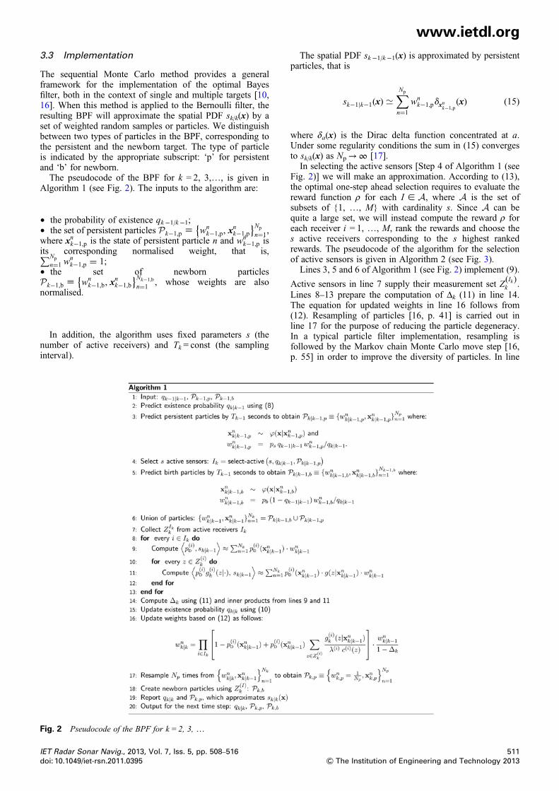
3.3 Implementation
The sequential Monte Carlo method provides a generalframework for the implementation of the optimal Bayesfilter, both in the context of single and multiple targets [10,16]. When this method is applied to the Bernoulli filter, theresulting BPF will approximate the spatial PDF sk|k(x) by aset of weighted random samples or particles. We distinguishbetween two types of particles in the BPF, corresponding tothe persistent and the newborn target. The type of particleis indicated by the appropriate subscript: ‘p’ for persistentand ‘b’ for newborn.The pseudocode of the BPF for k = 2, 3,…, is given in

Algorithm 1 (see Fig. 2). The inputs to the algorithm are:

† the probability of existence qk−1|k−1;† the set of persistent particles Pk−1,p ;

{wnk−1,p, x

nk−1,p

}Np

n=1,

where xnk−1,p is the state of persistent particle n and wnk−1,p is

its corresponding normalised weight, that is,∑Npn=1 w

nk−1,p = 1;

† the set of newborn particlesPk−1,b ; wn

k−1,b, xnk−1,b

{ }Nk−1,b

n=1, whose weights are also

normalised.

In addition, the algorithm uses fixed parameters s (thenumber of active receivers) and Tk = const (the samplinginterval).

Fig. 2 Pseudocode of the BPF for k = 2, 3, …


The spatial PDF sk −1|k−1(x) is approximated by persistentparticles, that is

sk−1|k−1(x) ≃∑Np

n=1

wnk−1,pdxn

k−1,p(x) (15)

where δa(x) is the Dirac delta function concentrated at a.Under some regularity conditions the sum in (15) convergesto sk|k(x) as Np→∞ [17].In selecting the active sensors [Step 4 of Algorithm 1 (see

Fig. 2)] we will make an approximation. According to (13),the optimal one-step ahead selection requires to evaluate thereward function ρ for each I [ A, where A is the set ofsubsets of {1, …, M} with cardinality s. Since A can bequite a large set, we will instead compute the reward ρ foreach receiver i = 1, …, M, rank the rewards and choose thes active receivers corresponding to the s highest rankedrewards. The pseudocode of the algorithm for the selectionof active sensors is given in Algorithm 2 (see Fig. 3).Lines 3, 5 and 6 of Algorithm 1 (see Fig. 2) implement (9).

Active sensors in line 7 supply their measurement set ZIk( )

k .Lines 8–13 prepare the computation of Δk (11) in line 14.The equation for updated weights in line 16 follows from(12). Resampling of particles [16, p. 41] is carried out inline 17 for the purpose of reducing the particle degeneracy.In a typical particle filter implementation, resampling isfollowed by the Markov chain Monte Carlo move step [16,p. 55] in order to improve the diversity of particles. In line


Fig. 3 Active receiver selection pseudocode

www.ietdl.org

18 the newborn particles are created for the next cycle of theparticle filter. This is done for all z [ Z(I)

k using the accept–reject method [18]. First we draw samples from amultivariate Gaussian N (x; m, C), where μ and C are themean and covariance adopted so that target birth densitycovers the entire state space X . Then we accept only thosesamples whose velocity vector is compatible with theDoppler measurement z. For each measurement we createin this way Np/2 newborn particles, that isNk,b =

∣∣Z(I)k

∣∣× Np/2. The weights of newborn particles areuniform. In line 19 the algorithm reports the probability oftarget existence qk|k and the particle set Pk|k,p, whichapproximates sk|k(x). In addition, if qk|k≥ 0.5, the algorithmreports the mean and the covariance of Pk|k,p. Theseestimates will be used in the error performance assessment.An explanation of Algorithm 2 (see Fig 3) follows next. In

line 2 we create a sample of predicted particles of size L≪N.These particles are used in the for-loop from line 6–13 to forma sample of a reward function ρ. Each sample of the reward isbased on a ‘future measurement’ created in line 7 under the

Fig. 4 Simulation setup

a Target trajectory, the locations of receivers (blue squares) and the transmitter (reb Probability of detection as a function of the distance between the receiver and th


assumption that there are no false detections and probabilityof detection is 1. Line 12 follows from (14). Theexpectation operator in (13) is implemented in line 14 as asample mean. Finally, as we explained earlier, the rewardscorresponding to receivers are ranked in line 16 and thehighest s ranked receivers are selected.

4 Numerical results

4.1 Simulation setup with a single run

The BPF for multi-static Doppler-shift measurements is testedusing a scenario withM = 10 receivers placed in the x–y planeat locations shown in Fig. 4a. The emitter with transmittingfrequency fc = 900 MHz is placed at the origin of thex–y plane. The sampling interval is fixed to Tk = 2 s. Thetarget exists for discrete-time indices k = 4, 5,…, 40,with the true initial state vector x4 = [− 4 km 20m/s 7 km−25m/s]T and process noise parameter q = 0.01. All receiversi = 1,…,M are characterised by identical measurement noise

d star)e target


www.ietdl.org
standard deviations s(i)
w = sw = 2.5Hz, and false detection(clutter) parameters λ(i) = 2 and c(i)(z) = 1/400 Hz for z∈[− 200 Hz, 200 Hz] and zero otherwise. The probability ofdetection is modelled as follows

p(i)D xk( ) = 1− f pk − ri

∥∥ ∥∥; a, b( )(16)

where dk,i = ||pk− ri|| is the distance between the target and thesensor, f(d; a, b) = �d

−1 N (n; a, b) dn is the Gaussiancumulative distribution function with α = 15 km and β =(3 km)2. Fig. 4b plots the probability of detection (16) as afunction of the distance from a receiver.

Fig. 5 Single run of the algorithm

a Probability of existenceb True and estimated target trajectory with 2σ uncertainty ellipsoidsc OSPA error

Fig. 6 Mean OSPA error for the number of active receivers s = 1,2, 4 (σw = 2.5 Hz)


The BPF was implemented using the birth parameters m =[0 0 0 0]T, C = diag (4 km)2 (30m/s)2 (4 km)2 (30m/s)2

[ ],

with Np = 10000, pb = 0.02, ps = 0.98 and the initialprobability of existence q0 = 0. The average reward wascomputed using L = 100 samples.The results of a single run of the algorithm, using s = 2

active receivers at each time k, with measurement noisestandard deviation σw = 2.5 Hz, are illustrated in Fig. 5. Thetarget appears at k = 4 and the its existence is detectedquickly as the probability of existence jumps to 0.8 at k =5, see Fig. 5a. Once the target is localised, the receiversselected to be active are always close to the target.Although their probability of detection is 1, the probabilityof existence remains very stable at the value of 1. Thetarget disappears at k = 41 and the probability of existenceimmediately drops to a small value close to zero. The targettrajectory estimate, shown in Fig. 5b, approaches theground truth. The 2σ uncertainty ellipsoids (obtained fromthe covariance of Pk|k,p ) include at every instance the truetarget position.The estimation accuracy of the BPF is measured using

the optimal sub-pattern assignment (OSPA) error metric[19]. This metric penalises both the cardinality estimateerror and the target location estimate error. In ouranalysis, we adopt the following parameters of the OSPAmetric: p = 1 (so that the OSPA error represents the sumof the localisation error and the cardinality error); c = 8km (the penalty assigned to the cardinality error). TheOSPA error for the single run of the algorithm is shownin Fig. 5c. Note that the OSPA error has high values for4 ≤ k ≤ 10; the source of the error at k = 4 is thecardinality error; after that the source of error is thelocalisation error. From Fig. 5c it was observed that withs = 2 it took only six discrete-time steps for the algorithmto localise the target.

4.2 Error performance analysis

An average error performance was estimated using the meanOSPA error (averaged over 20 Monte Carlo runs) andanalysed for three comparative studies as follows.

4.2.1 Study 1: The influence of s: Recall that thenumber of active receivers at each measurement


Fig. 8 Mean OSPA error for σw = 2.5 Hz and σw = 10 Hz (s = 1)

www.ietdl.org
acquisition time has been denoted by s. Fig. 6 shows theaverage OSPA error for s = 1, 2, 4 active receivers, withthe y-axis in the log-scale (when the mean OSPA is zero,the values are not shown). The selection of activereceivers was based on the information gain-basedapproach described in Section 3.2. Fig. 6 demonstratesthat, in accordance with our intuition, using more activereceivers at each time k, the mean OSPA reduces morequickly and to a lower value of the steady-state error. It isimportant to emphasise, however, that even for s = 1, thealgorithm is capable of establishing the presence of thetarget and eventually localising and tracking it. At k = 41and 42, when target is absent, we observe that on someMonte Carlo runs the probability of existence qk|kremained above the threshold 0.5.
4.2.2 Study 2: The significance of receiverselection: In order to establish the importance of activereceiver selection, we compare the information gain-basedapproach described in Section 3.2 against the randomselection of receivers. The results using s = 1 and 4 activereceivers are shown in Fig. 7. From this figure one canobserve that, irrespective of s, the information gain-basedselection results in somewhat faster convergence and a

Fig. 7 Mean OSPA error using information gain-based selectionagainst random selection of receivers (σw = 2.5 Hz)

a s = 1b s = 4


lower value of the steady-state error. It is noteworthy that,in the described setup, even the random selection results insuccessful detection and tracking of a target, albeit withhigher error.

4.2.3 Study 3: The influence of Dopplermeasurement error: Fig. 8 shows the mean OSPA errorfor two values of the Doppler measurement noise standarddeviation: σw = 2.5 Hz and σw = 10 Hz. Both curves wereobtained using s = 1 active receiver at each update step.The higher value of σw affects both the target detectionperformance (it takes more scans to detect the presence anddisappearance of the target) and the localisation error (thelocalisation error in the steady state, that is, between k = 35and 40, is increased from 130 m to ∼500 m).

4.2.4 Discussion: Overall, the described BPF isremarkably reliable, even using only s = 1 active receiverat each time and selecting the receivers at random. TheBernoulli filter in general is fairly robust to divergence: ifit cannot localise correctly the target, the probability ofexistence drops and as a consequence the filter givesmore emphasis to received measurements (via birthdensity). Effectively, when probability of existence is low,the filter automatically operates in a search mode, whicheventually results in correct localisation and tracking.Using more instantaneously active receivers and applyingthe information gain-based receiver selection, improves theperformance: both of these actions speed up the filterconvergence and result in a lower steady-state error. TheBernoulli filter can divergence only as a consequence ofits inefficient particle filter implementation or insufficientnumber of particles used. The price of robustperformance, however, is that the proposed BPF withinformation-based receiver selection is computationallyvery intensive. Since the Doppler-only measurements arefairly uninformative (especially for small s), the posteriorPDF is diffuse during several initial time steps, meaningthat it is necessary to use a large number of particles tocover the state space (particularly problematic is targetposition, being initially unobservable). Information gainreceiver selection is computationally very expensive: ourMATLAB implementation of the BPF with informationgain selection is three times slower than with randomselection. The effect of s on computational complexity isnegligible.


www.ietdl.org
5 Conclusions
This paper presented a recursive Bayesian algorithm for jointdetection and tracking of a single target using multi-staticDoppler-only measurements contaminated by falsedetections and miss-detections. The proposed algorithm isnot only capable of processing both the synchronous andasynchronous measurements, but also to select the mostinformative transmitter–receiver pairing, as the target movesacross the surveillance plane. The algorithm has beenimplemented using the sequential Monte Carlo method, as aparticle filter. The numerical simulations demonstrated thatit reliably detects and tracks a target. As expected, usingsynchronous measurements from multiple receiversimproves the performance. Future work will consider themultiple-target case, the learning of clutter statistics [20]and more efficient particle filter implementations.Experiments similar to those reported in [21] are alsoenvisaged.

6 References

1 Peterson, A.M.: ‘Radio and radar tracking of the Russian Earth satellite’,Proc. IRE, 1957, 45, (11), pp. 1553–1554

2 Salinger, S.N., Brandstatter, J.J.: ‘Application of recursive estimationand Kalman filtering to Doppler tracking’, IEEE Trans. Aerosp.Electron. Syst., 1970, 4, (4), pp. 585–592

3 Chan, Y.-T., Jardine, F.: ‘Target localization and tracking fromDoppler-shift measurements’, IEEE J. Ocean. Eng., 1990, 15, (3), pp.251–257

4 Torney, D.C.: ‘Localization and observability of aircraft viaDoppler-shifts’, IEEE Trans. Aerosp. Electron. Syst., 2007, 43, (3),pp. 1163–1168

5 Xiao, Y.-C., Wei, P., Yuan, T.: ‘Observability and performance analysisof bi/multi-static Doppler-only radar’, IEEE Trans. Aerosp. Electron.Syst., 2010, 46, (4), pp. 1654–1667

6 Shames, I., Bishop, A.N., Smith, M., Anderson, B.D.O.: ‘Analysis oftarget velocity and position estimation via Doppler-shiftmeasurements’. Proc. Australian Control Conf., Melbourne, Australia,November 2011, pp. 507–512

7 Dargie, W., Poellabauer, C.: ‘Fundamentals of wireless sensor networks:theory and practice’ (Wiley, 2010)

8 Webster, R.J.: ‘An exact trajectory solution from Doppler shiftmeasurements’, IEEE Trans. Aerosp. Electron. Syst., 1982, 18, (2),pp. 249–252

9 Jazwinski, A.H.: ‘Stochastic processes and filtering theory’ (AcademicPress, 1970)

10 Mahler, R.: ‘Statistical multisource multitarget information fusion’(Artech House, 2007)

11 Vo, B.-T., See, C.-M., Ma, N., Ng, W.-T.: ‘Multi-sensor joint detectionand tracking with the Bernoulli filter’, IEEE Trans. Aerosp. Electron.Syst., 2012, 48, (2), pp. 1385–1402

12 Ristic, B., Arulampalam, S.: ‘Bernoulli particle filter with observercontrol for Bearings-Only tracking in clutter’, IEEE Trans. Aerosp.Electron. Syst., 2012, 48, (3), pp. 2405–2415

13 Bar-Shalom, Y., Li, X.R., Kirubarajan, T.: ‘Estimation with applicationsto tracking and navigation’ (John Wiley & Sons, 2001)

14 Castanón, D.A., Carin, L.: ‘Stochastic control theory for sensormanagement’, in Hero, A.O., Castanón, D.A., Cochran, D., Kastella,K. (Eds.): ‘Foundations and applications of sensor management’(Springer, 2008), Ch. 2, pp. 7–32

15 Kailath, T.: ‘The divergence and Bhattacharyya distance measures insignal selection’, IEEE Trans. Commun. Technol., 1967, 15, (1), pp.52–60

ck Z(i)k |X

( )=

k Z(ik

(

k Z(i)k

( )1− p(i)D (x)+ p(i)D (x)

z

⎛⎝

⎧⎪⎪⎪⎪⎨⎪⎪⎪⎪⎩


16 Ristic, B., Arulampalam, S., Gordon, N.: ‘Beyond the Kalman filter:particle filters for tracking applications’ (Artech House, 2004)

17 Crisan, D., Doucet, A.: ‘A survey of convergence results on particlefiltering methods for practitioners’, IEEE Trans. Signal Process.,2002, 50, (3), pp. 736–746

18 Robert, C.P., Casella, G.: ‘Monte Carlo statistical methods’ (Springer,2004, 2nd edn.)

19 Schuhmacher, D., Vo, B.-T., Vo, B.-N.: ‘A consistent metric forperformance evaluation of multi-object filters’, IEEE Trans. SignalProcess., 2008, 56, (8), pp. 3447–3457

20 Vo, B.-T., Vo, B.-N., Hoseinnezhad, R., Mahler, R.P.S.:‘Multi-Bernoulli filtering with unknown clutter intensity and sensorfield-of-view’. Proc. 45th Conf. Information Sciences and Systems(CISS), 2011

21 Guldogan, M.B., Lindgren, D., Gusafsson, F., Habberstad, H., Orguner,U.: ‘Multiple target tracking with Gaussian mixture PHD filter usingpassive acoustic Doppler-only measurements’. Proc. Int. Conf.Information Fusion, Singapore, July 2012

7 Appendix

The derivation of (10)–(12) follows the steps in [10, Sec.G.24]. The PDF of a Bernoulli RFS X is updated at time kusing the Bayes rule as

fk|k X |Z Ik( )k , Z1:k−1

( )=

ck ZIk( )

k |X( )

fk|k−1 X |Z1:k−1

( )�ck Z

Ik( )k |X

( )fk|k−1 X |Z1:k−1

( )dX

(17)

where ck

(Z

Ik( )k |X) is the multi-sensor likelihood function and

fk|k−1 X |Z1:k−1

( )is the predicted PDF completely specified by

the pair qk|k−1, sk|k−1(x)( )

via (7), with qk|k−1 and sk|k−1(x)computed according to (8) and (9), respectively. Theintegral in the denominator of (17) is the set integral [10],for which the Bernoulli RFS X takes the form

∫f (X )dX = f (∅)+

∫f (x) dx

.Assuming the sensor measurements are conditionallyindependent, we can write for the likelihood

ck ZIk( )

k |X( )

=∏i[Ik

ck Z(i)k |X

( )(18)

where [10, p. 517] (see (19))Here, κ(Z ) is the PDF of the false measurement set Z.According to the model adopted in Section 2, the falsedetection RFS Z(i)

k is a Poisson process with the PDF [10,

Eq. (12.51)]: k(Z(i)k

) = el(i) ∏

z[Z(i)k

[l(i) c(i)(z)

]. Then the

ratio k(Z(i)k \{z})/k(Z(i)

k

), which features in (19), simplifies

to l(i) c(i)(z)( )−1

.

)), if X = ∅

∑[Z(i)k

g(i)k (z|x) k Z(i)k \{z}

( )k Z(i)

k

( )⎞⎠, if X = {x}

(19)


www.ietdl.org
Now it is straightforward to show that the denominator of
(17) can be expressed by (20).When X = ∅, from (17), (20) and the definition of the PDF

of a Bernoulli RFS (7), we obtain (21).

∫ck Z(Ik )

k |X( )

fk|k−1 X |Z1:k−1

( )dX =

∏i[Ik

k Z(i)k

( )1− qk|k−1 + q

{

1− qk|k =∏

i[Ikk Z(

∏i[Ik

k Z(i)k

( )1− qk|k−1 + qk|k−1

∏i[Ik

1

[{


The terms∏

i[Ikk(Z(i)k

)in (21) cancel out and after some

rearrangements we obtain (10). Similarly, from X = {x}case, using (7), (17) and (20), it is straightforward to derive(12).

k|k−1

∏i[Ik

1− kp(i)D , sk|k−1l[

+∑z[Z(i)

k

k p(i)D g(i)k (z| · ), sk|k−1ll(i)c(i)(z)

] (20)

(i)k

)1− qk|k−1

( )− kp(i)D , sk|k−1l+

∑z[Z(i)k

k p(i)D g(i)k (z| · ), sk|k−1ll(i)c(i)(z)

]} (21)


target tracking via multi-static doppler shifts

Documents