Taper Tantrums: QE, its Aftermath and Emerging Market Capital Flows1,2

Anusha Chari UNC-Chapel Hill &

NBER

Karlye Dilts Stedman UNC-Chapel Hill

Christian Lundblad UNC-Chapel Hill

November 2017

Abstract

This paper provides a novel perspective on the impact of U.S. unconventional monetary policy (UMP) on emerging market capital flows and asset prices. An affine term structure model shows that U.S. monetary policy shocks, identified with high-frequency Treasury futures data, represent revisions to the expected path of short-term interest rates and the required risk compensation that is especially significant during the UMP period. The policy shocks exhibit sizable effects on U.S. holdings and valuations of emerging market assets with larger effects for asset returns relative to physical flows, equity relative to fixed income markets, and during the taper period. Keywords: Unconventional monetary policy, international spillovers, emerging markets, high frequency identification, affine term structure model, portfolio flows, asset valuations.

1 Contact: achari@unc.edu, kdilts@live.unc.edu, Christian_Lundblad@kenan-flagler.unc.edu. We thank seminar participants at the 14th NIPFP-DEA conference, Kesroli, Rajasthan, UNC-Chapel Hill, ISB’s Summer Research Conference, 2016, the IMF, the 2017 AEA meetings, the Darden School at UVA, the NBER’s IFM meeting, the 2017 Western Finance Association meeting, the Society for Economic Measurement annual symposium, the Bank of Canada, the Bank of Korea, Tsinghua University, and the XX IEF Workshop, UTDT, Buenos Aires. We also thank Frank Warnock, Winston Duo, Prachi Mishra, Jay Shambaugh, Joshua Aizenman, Linda Goldberg, Lars Hansen, Guillermo Mondino, Hongjun Yan, Antonio Diez de los Rios, and VV Chari for many helpful comments and suggestions. 2 Disclosure Statements: “I have nothing to disclose” (Anusha Chari). “I have nothing to disclose” (Karlye Dilts-Stedman). “I have nothing to disclose” (Christian Lundblad).

2

1. Introduction

The massive surge of foreign capital to emerging markets in the aftermath of the

global financial crisis (GFC) of 2008–2009 has led to a contentious debate about the

international spillover effects of developed-market monetary policy with particular

emphasis on the United States (Fratzscher, Lo Duca, and Straub 2013; Rey 2014). The

monetary policy decisions of the U.S. Federal Reserve during the crisis had a primarily

domestic focus to stimulate growth in its aftermath. However, these policy actions led to

substantial spillover effects for emerging-market economies (Fratzscher, Lo Duca, and

Straub 2013). As interest rates in developed economies remained low, investors were

attracted to the higher rates in many emerging economies (Fratzscher 2012).

The surge in foreign capital led Brazilian President Dilma Rousseff to evocatively

claim that advanced economy monetary policy had unleashed a “monetary tsunami” in

the developing world.3 The governor of Taiwan’s central bank, Perng Fai-Nan echoed

this sentiment, “The U.S. printed a lot of money, so there’s a lot of hot money flowing

around. We see hot money in Taiwan and elsewhere in Asia … These short-term capital

flows are disturbing emerging economies.” Later, announcements by the Fed suggesting

that an unwinding of quantitative easing was imminent appeared to trigger a selloff in

emerging markets; “taper talk” led to considerable speculation about dollar-funding

conditions tightening and financial stability concerns in emerging economies.

We examine the effects of (unconventional) U.S. monetary policy on emerging

market capital flows and asset prices using a relatively recently developed technique to

identify policy shocks. We exploit the development of a budding literature on the use of

high-frequency data to identify monetary policy shocks to more precisely address the

magnitude of any attendant spillover effects. With this technology, we can further

decompose and quantify these effects using a dataset on global capital flows and

positions from the U.S. Department of Treasury to capture U.S. investment positions in

emerging market asset markets and their valuations. While previous studies use these

data in other contexts,4 this paper sheds new light on the link between U.S. monetary

policy shocks, net capital flows, and emerging market equity and bond market returns.

3 http://articles.economictimes.indiatimes.com/2012-03-28/news/31249809_1_india-and-brazil-brazil-today-brazilian-president-dilma-rousseff 4 Examples include Curcuru et al (2010) and Bertaut, Griever and Tryon (2006).

3

Our first step is to identify monetary policy shocks at the zero lower bound (ZLB)

— and the task is not straightforward. For example, as Christiano, Eichenbaum, and

Evans (1999) make clear; the literature has not converged on a unifying set of

assumptions to identify exogenous shocks to monetary policy even for the pre-crisis

period. The primary methods of identifying monetary policy shocks in the literature fall

into three general categories. They are (i) panel estimation with announcement dummies

(Fratzscher, Lo Duca and Straub 2013; Ahmed and Zlate 2014;), (ii) structural VARs

(Zha 1997; Dedola, Rivolta, and Stracca, 2015), and (iii) high-frequency identification

(HFI) schemes (Gilchrist, Yue and Zakrajsek 2014; Neely 2010; Mishra, Moriyama,

N'Diaye and Nguyen 2014). Although the particular details vary, the benefits of each

methodology lie in the data used for monetary policy shock identification and usually

depend on the frequency of the chosen data.

As mentioned above, we follow the rapidly growing set of papers that employ

high-frequency identification of monetary policy shocks by extracting the unexpected

component from Treasury futures contracts. While expectations of Fed policy actions are

not directly observable, futures prices are associated with a traded derivative contract,

providing a “market-based proxy” for these expectations (Kuttner 2001). Given that

actual rate changes were largely absent during most of the crisis and post-crisis periods,

the Fed has relied heavily on forward guidance to manage expectations about future Fed

policy. During the QE period, FOMC statements, for the most part, worked to manage

expectations that the policy rate would continue near the ZLB and had an explicit goal of

influencing longer-term interest rates. Changes in the price of derivatives contracts such

as Treasury futures can therefore reflect changes in the perceived probability of future

Fed policy. In this setting, we follow Rogers, Scotti, and Wright (2014) to measure

monetary surprises at the ZLB as the change in futures-implied yields bracketing FOMC

announcements. Having extracted these policy shocks, we regress measures of net capital

flows and asset returns on the extracted shocks in a panel setting to more precisely gauge

the degree to which emerging markets are affected by U.S. monetary especially,

unconventional policy.

Before proceeding, it is important to recognize that during ordinary times,

monetary policy can generate spillovers to emerging markets through conventional

channels (Kim 2001; Obstfeld and Rogoff 1995). However, additional transmission

channels are possible because the period of unconventional monetary policy has involved

4

heavier management of expectations and efforts to exert direct control further along the

yield curve.5 A unifying question is the degree to which monetary shocks represent

revisions in market participants’ expectations about the path of short-term interest rates

and / or changes in their required risk compensation. To interpret the nature of the

shocks extracted from the Treasury bond futures market, we use a common affine term

structure model (see Kim and Wright 2005). We find that our monetary policy shocks, in

part, represent revisions in expectations about short-term interest rates, but even more

significantly, they capture changes in required risk compensation. The important role for

time-varying risk compensation is particularly true during the period of unconventional

monetary policy.

Using panel data and high-frequency identification, we then turn to our main

contribution. We examine the impact of measured, high-frequency U.S. monetary policy

surprises around FOMC meetings on capital flows from the United States to a range of

emerging markets as well as the associated emerging market valuations. The benchmark

specification estimates the impact of monetary surprises for both equity and debt

instruments as a percent of annual GDP for: (i) total positions, (ii) valuation changes

(e.g., returns) and (iii) capital flows, as well as an examination of any attendant exchange

rate effects.

Our results reveal heterogeneity along three principal lines: flows versus prices,

debt versus equity, and quantitative easing versus tapering. Among these, the most robust

finding is that valuation changes for both debt and equity played a key role in the change

in overall positions observed between sub-periods. That is, in nearly every specification,

the effect of monetary policy shocks on asset returns is larger than that for physical

flows. This finding is consistent with the notion that our shocks may capture a revision in

required risk compensation across financial markets.

Second, we also find that (scaled) equity positions and valuations are more

sensitive to monetary policy shocks—across three sub-periods, equity valuation effects

are an order of magnitude larger than debt valuation effects. During the QE period, for

instance, the coefficient on equity valuations in response to a monetary policy shock is

approximately ten times higher than the coefficient on debt valuations.

5 See Fratzscher et al 2014 for a comprehensive summary.

5

Third, while we detect some significant effects of monetary policy on flows and

valuations during the QE period, the effects are not consistent over all dependent

variables. However, during the period following the first mention of asset purchase

tapering, we find a consistent and large effect of monetary policy shocks on nearly all

variables of interest. In particular, we find that the effects of monetary policy on debt

flows during the taper period are much higher and statistically significant than during the

QE period. In some cases, such as for debt valuations, the impact of monetary policy

shocks in the taper period is an order of magnitude above the coefficient in the QE

period.

The coefficient estimates on the monetary surprise measures during the taper

period suggest that the market interpreted the unwinding of unconditional monetary

policy as a signal that normalcy was being restored to the U.S. economy and, consistent

with both the signaling and portfolio balance channels, expected monetary tightening in

the U.S. both in the near-term and ongoing in the future led to a massive retrenchment

from emerging markets.

A significant advantage of extracting the magnitude of the monetary surprises

directly from futures data is that we can estimate a dollar amount in terms of the changes

in U.S. investor positions and flows into emerging markets, controlling for a variety of

push and pull factors. Previous studies that use period indicator variables or alternative

approaches to examine U.S. monetary policy spillovers are only able to make qualitative

statements about the direction of impact. In contrast, using derivatives price changes we

can quantify the impact of U.S. monetary policy on emerging market capital flows

depending on the magnitudes, signs, and dispersion of the extracted monetary policy

shocks. A richer picture emerges from our approach, whereby we can make distributional

predictions that are more in line with emerging markets’ varied experience across both

markets and time periods.

Our paper is related to previous studies that examine the effect of unconventional

monetary policy on capital flows using panel data on emerging markets by including

indicators for the dates of FOMC meetings and speeches by the Fed Chair, along with a

number of fundamental control variables (Fratzscher, Lo Duca and Straub 2013; Ahmed

and Zlate 2014; Aizenman, Binici and Hutchison 2014). The main findings in the

literature suggest that quantitative easing in the U.S. was an important driver of capital

flows into emerging economies (Ahmed and Zlate 2014), although the effects varied

6

across episodes and importantly, the impact of QE on asset prices was greater than that

on flows (Fratzscher, Lo Duca and Straub 2013).

Event studies that use high-frequency identification suggest that U.S.

unconventional monetary policy had a significant effect on interest rates in both

advanced and emerging economies. Focusing on both the QE and taper periods, Mishra,

Moriyama, N'Diaye and Nguyen (2014) find that taper talk had a significant effect on

bond yields, exchange rates, and equity prices, but that better country fundamentals and

stronger trade ties with China mitigated the effect. Karolyi and McLaren (2016) show

that the initial tapering announcement in 2013 had negative valuation impacts overall, but

that emerging market stocks with larger positive cumulative abnormal returns around

earlier LSAP purchase announcements were particularly hard hit in 2013. Our nearest

neighbor in this literature uses factor analysis to separate market and signal factors from

changes in bond yields around FOMC events, finding that unconventional monetary

policy surprises had larger effects on equity prices, exchange rates, bond yields and

mutual fund flows than those during conventional periods, finding additionally that

“signal” shocks—those that portend the path of future interest rates—generate larger and

more ubiquitous spillovers (Chen et al. 2014).

The paper proceeds as follows. Section 2 briefly describes the related literature on

U.S. monetary policy and capital flows to emerging markets with an emphasis on

identifying monetary policy shocks and measuring spillovers at the zero lower bound.

Section 3 presents our methodology for extracting monetary policy surprise measures

using high-frequency identification and explores their relationship to revisions in

expectation about future short rates and term premia. Section 4 describes the data and

methodology for measuring capital flows and presents summary statistics. Section 5

presents the benchmark specification and the regression results along with robustness

checks and alternative tests. Section 6 concludes.

2. Related Literature

The literature on the pattern of international capital flows separates determinants

into push factors which are common, global factors associated with external shocks, and

pull factors, which are country-specific. Push factors alter the relative attractiveness of

investing in developed countries. Global volatility (the VIX is an often employed proxy),

global liquidity, global interest rates and global growth are considered push factors—

7

their variation is thought to drive phenomena such as search for yield or flight to safety

which may affect developed market flows to or from emerging economies (Calvo et al

1993). There is strong evidence in the literature for the impact of global risk aversion and

developed-economy interest rates, and there is some evidence for the effect of advanced-

economy output growth (Fratzscher 2012; Fratzscher et al 2014; Passari and Rey 2015;

Milesi Ferretti and Tille 2011; Broner et al 2013; Forbes and Warnock 2012).

Pull factors, on the other hand, change the risk-return characteristics of emerging-

market assets. These include country characteristics such as financial sector development,

domestic interest rates and asset returns, integration with global financial markets, fiscal

position and domestic growth shocks. While the balance of evidence suggests that push

factors are a more powerful determinant of capital flows, there is some evidence that

domestic output growth, domestic interest rates or asset returns and country risk

indicators have an impact on capital flows, as well (Ahmed and Zlate 2013; Fratzscher

2012).6

A third set of factors that fall partially under each of the previous two are related

to contagion, trade linkages, financial linkages and location, which may also play a role

in driving portfolio and banking flows. These are addressed in a separate literature on

financial contagion. Although we do not focus on contagion directly, by measuring the

impact of U.S. monetary policy on flows to and from a broad set of emerging markets,

we are attempting to identify the size of flows induced by a global financial shock.

2.1 U.S. Monetary Policy and Capital Flows to Emerging Markets: Spillovers at the

Zero Lower Bound

The period of unconventional monetary policy has involved a heavier

management of expectations and efforts to exert direct control further along the yield

curve. Additional channels of monetary policy transmission in operation include the

portfolio balance, signaling, confidence, and liquidity channels (Krishnamurthy and

Vissing-Jorgensen 2011; Neely 2010; Fratzscher 2012; Fratzscher et al 2014; Lim et al

2014). Based on the usual decomposition of yields on safe long-term government bonds,

there are two potential elements of the yield curve that central bank bond purchases can 6 Capital flows driven by pull factors may be more desirable when the intrinsic quality of these assets attracts foreign investors, as they may be more committed to these positions and less likely to unwind them quickly.

8

affect: the average level of short-term interest rates over the maturity of the bond and the

term premium. Specifically, consider the yield on an n-year bond as decomposed in the

asset pricing literature: as the average of expected overnight rates over the life of the

bond and a term premium:

Yt;t+n =Yt:t+nEH +YTPt;n (1)

where Yt:t+nEH is the average short term rate expected over the period t to t+n (that is, the

component of the yield that would drive yield variation if the expectations hypothesis

were to hold), and YTPt;n is a maturity-specific term premium. We next address each

potential channel's relationship to this yield decomposition in turn.

First, the portfolio balance channel results from a confluence of forces.

Quantitative easing involves the purchase of longer-duration assets, which reduces the

effective supply of such assets to private investors, thereby raising their price and

lowering yields. As investors rebalance their portfolios in response to quantitative easing,

the prices of the assets they buy should rise as well, decreasing their respective yields.7

Thus, we can expect that, if the portfolio balance channel dominates, a loosening of

monetary policy via quantitative easing will result in increased flows to emerging

markets as investors substitute toward emerging-market assets in search of higher yields.

Likewise, we would expect that a contractionary monetary policy incentivizes investors

to rebalance in favor of U.S. Treasuries. Thus, if the portfolio channel is in operation we

expect that monetary policy shocks will be inversely correlated with emerging market

flows and valuations.

Additionally, if investors demand a premium for holding longer-term bonds, then

the term premium (YTPt;n above) will also be influenced by the relative supply of long

term assets. If the Fed removes long-term securities from the market, i.e. duration risk,

investors should require a smaller premium to hold the reduced quantity of long-term

securities. Overall yields can fall once again prompting a rebalancing toward higher yield

emerging market assets.

Although quantitative easing does not directly affect short-term interest rates, it

may serve as a signal to markets regarding the future path of interest rate policy. This

signaling channel can operate as follows. If taken as a commitment by the Fed to keep

7 http://www.federalreserve.gov/newsevents/speech/bernanke20120831a.htm

9

future policy rates lower than previously expected, the signaling channel would suggest

lower yields associated with a lower the average expected short-rate, Yt:t+nEH in equation (1)

(Fratzscher et al 2014; Neely 2010; Lim et al 2014).

In the context of emerging market capital flows, the ongoing large scale asset

purchases (LSAPs) can signal that large interest rate differentials between advanced

economy yields with respect to emerging markets are expected to persist. In the literature

on capital flows, the interest rate differential may trigger a carry trade, resulting in

sizeable capital flows into emerging markets (Galati, Heath and McGuire 2007). As in

the case of the portfolio balance channel, we would expect the coefficient on a monetary

policy shock dominated by the signaling channel to be negative.

The confidence channel of unconventional monetary policy is closely related to

the signaling channel and can influence portfolio decisions and asset prices by altering

the risk appetite of investors. For example, an announcement of tapering might serve as a

signal that the FOMC is feeling sanguine about global economic prospects, lowering

relative risk aversion and, consistent with predictions from the literature on capital flow

determinants, increasing capital flows to emerging markets. Reduced confidence, in

contrast, can lead to capital outflows from emerging markets or a flight to safety. We

would thus expect a loosening monetary policy shock dominated by the confidence

channel to drive capital outflows from emerging markets.

Quantitative easing can also affect portfolio decisions and asset prices by altering

the liquidity premium (Krishnamurthy and Vissing-Jorgensen 2011; Neely 2010), and

thus the efficiency of markets. In practice, LSAPs are credited in the form of increased

reserves on private bank balance sheets (Krishnamurthy and Vissing-Jorgensen 2011).

Since such reserves are more easily traded in secondary markets than are long-term

securities, the liquidity premium decreases. Thus, liquidity-constrained banks can extend

credit to borrowers, resulting in decreased borrowing costs and elevated lending levels.

However, before we can identify the various channels through which unconventional

monetary policy operates, we must first identify it.

10

3. Extracting Monetary Policy Surprise Measures Using High-Frequency

Identification

Using high frequency identification allows us to make several unique

contributions to the literature on the spillover effects of U.S. monetary policy on

emerging market capital flows. For example, panel estimation using dummies only for

event dates thought to contain a surprise Treasury rate change may fail to include dates

that are not widely-recognized as surprises or may miss dates that contain a surprise

insofar as rates did not change. Similarly, studies that use simple changes in the Treasury

yields may lead to an attenuated estimated monetary policy effect if the lack of any

change is itself a surprise. Finally, using dummies to identify a monetary policy shock

obscures the magnitude of the shock. Using high-frequency identification and

conditioning on the magnitudes of the monetary surprises we are able to quantify the

impact on capital flows to emerging markets.

The abundance of short-term interest rates that potentially measure federal funds

rate expectations has led to a proliferation of asset price-based monetary policy

expectation measures emanating from Kuttner (2001). Among the short-term variables

found in use in this literature are the current-month federal funds futures contract price,

the month-ahead federal funds futures contract price, the one-month Eurodollar deposit

rate, the three-month Treasury bill rate, and the three-month Eurodollar futures rate.

Gürkaynak, Sack and Swanson (2005, 2007) and Gürkaynak (2005) propose

alternative shock measures that capture changes in market expectations of the policy rate

over slightly longer horizons. Since December 2008, however, there have been almost no

changes in the target federal funds rate, and, until recently, FOMC statements for the

most part worked to maintain the perception that the policy rate would continue near

zero. In this setting, and in light of QE`s explicit goal of influencing longer-term interest

rates, we use a measure of monetary policy shocks at the ZLB as in Rogers, Scotti and

Wright (2014). Following their methodology, we measure U.S. monetary policy surprises

as the change in futures-implied yields bracketing FOMC announcements. Specifically,

the surprise is the daily change in five-year Treasury futures on the date of FOMC

announcements.

11

To construct our baseline monetary policy shocks, we used the daily difference in

the implied yield of the five-year Treasury bond futures contract on potential dates for

monetary policy surprises.8 The majority of our dates are FOMC meetings and

conference calls from the Federal Reserve Board website,

https://www.federalreserve.gov/monetarypolicy/fomccalendars.htm. The remaining

events are taken from Gagnon et al (2011) and Fratzscher er al (2013). Finally, we

include the “Taper Tantrum” episode of May 22, 2013.

Table 1 displays summary statistics for our main monetary policy shock measure

and for three additional robustness measures, including correlations among the various

measures. The data underlying our monetary policy shock measures are expressed in

percentage points. Thus, for example, the average daily change in the implied yield on

five-year Treasury Futures during the QE (Taper) period is a decrease (increase) of 2.0

(1.7) basis points, in contrast to a -0.4 basis point average daily change in the contract

over the full sample and a -0.3 basis point change in the pre-GFC period. Table 1 also

includes the significance levels from a simple test of means between periods; hence, the

differences in period averages between our dates of interest are statistically significant.

Figure 1 shows the five-year Treasury Futures yield changes on FOMC event dates.

Table 1 also includes several alternative high-frequency measures of monetary policy

shocks that we consider in Section 5.9

3.1 Understanding the Monetary Surprise Measures

In order to understand the manner in which our monetary policy shocks affect

global flows and valuations, we first need to better understand the nature of the revisions

in expectations housed in our variable. As mentioned, monetary policy potentially

influences both the expected path of short-term interest rates and the term premium.

However, from mid-2008 until as recently as mid-2015, the Fed was not expected to

deviate from zero short-term interest rates; it is not unreasonable, therefore, to suspect 8 Although a number of contracts satisfy the identifying assumptions needed to extract a surprise, we converge on five-year bond futures for a number of reasons, the first is precedence in the literature (see Rogers, Scotti and Wright 2014). Furthermore, using the five-year bond futures allows for us to extract a monetary policy shock that exhibits variation in both the conventional and unconventional monetary policy periods, wherein the latter period it accounts for the explicit targeting of long-term interest rates by the Federal Reserve. 9 For robustness, we examine a variety of monetary policy shocks extracted from different futures instruments such as the one- and two-month Fed Funds futures contracts as well as the changes in the two-year Treasury bond yields and intra-daily bond yield changes. Results are available upon request.

12

that monetary policy is qualitatively different in the periods of QE and of LSAP tapering

in the sense that the relationship between monetary policy and the term structure of

interest rates is altered. In this section of the paper, we explore the relationship between

our monetary policy surprise measure and the decomposition of the yield curve into a

component associated with the expected path of the short interest rate and that associated

with the term premium. This disaggregation permits an evaluation of the role for

monetary policy surprises across the conventional and unconventional periods.

We appeal to a well-established affine term structure methodology from Kim and

Wright (2005) that permits the decomposition of various government bond yields into

information about future short rates and term premia. Kim and Wright estimate a

standard latent three-factor Gaussian term structure model using zero-coupon Treasury

yields from the Gurkaynak, Sack, and Wright (GSW, 2007) database. To facilitate

empirical implementation, forecast data on the three-month T-bill yield from Blue Chip

Financial Forecasts are incorporated into the model estimation. Their model yields a

point-in-time daily estimate of the expected short rate over the life of any longer dated

bond as well as the risk compensation market participants require for holding that bond.10

To use these components, we separately regress changes (1) in bond yields, (2) in

the expected path of the short rate, and (3) in the term premium onto our monetary policy

shock to assess its importance on each. We conduct these separate regressions for one,

five and ten-year maturity U.S. Treasury bonds, separating the MP shock effects of

interest (those arising on relevant FOMC or policy announcement days) across three

periods (pre-crisis, March 1994 – August 2008, QE, December 2009 – April 2013, and

tapering, May 2013 – June 2016) 11:

10 The Kim and Wright yield curve decomposition data are made available at http://www.federalreserve.gov/pubs/feds/2005/200533/200533abs.html11 The pre-crisis dummy is equal to one in the period March 1994 to July 2008 and zero otherwise. The QE dummy is equal to one from the period December 2009 to April 2013. The Taper dummy is equal to one for the period after May 2013 when Ben Bernanke first mentioned the possibility of tapering LSAP purchases. The period between the collapse of Lehman Brothers and the beginning of QE was marked by global “flight to safety” and its inclusion in either neighboring sub-period contaminates the analysis in that it is a period of extraordinary uncertainty and cannot clearly be classified as the QE or the conventional periods. To ensure that we isolate the “flight to safety” flows, we include in our robustness checks and specification wherein the QE dummy begins on March 2009, as March 2009 marks the month during which equity markets in the United States began their recovery. While the quantitative effects for the emerging equity markets and exchange rates are smaller, we continue to observe statistical and economic significance. Results are available upon request. .

13

ΔY(n),t =α0 +β1dummypreMPt +β2dummyQEMPt +β3dummytaperMPt +εt (5)

Where the left-hand side variable Y(n),t is either the zero coupon bond yield on an n year

bond, the expectations hypothesis-implied average short rate component of an n year

bond, or the term premium on an n year bond. We consider two event windows for the

changes in the dependent variables – a daily change for event days perfectly coinciding

with the day of the MP shock, and a two-day change that includes the event day plus the

following to capture any relevant slow moving market effects.12 We provide

White standard errors to correct for heteroskedasticity (in parentheses). Finally, we allow

the monetary policy shock coefficients to vary across the three periods.

Table 2 (Panel A) shows the daily regressions for the overall yield change, the

change in the path of the expected short rate, and the change in the term premium, and

Panel B shows two-day yield change regressions for the same event dates. First, focusing

on the coefficients associated with the conventional, pre-crisis period, we find that a

positive FF5 shock is significantly associated with bond yield changes across maturities

both for the one-day event (Panel A) and the two-day event window (Panel B), though

this effect appears to diminish with the 10-year bond across both event windows. To

provide a sense of the economic magnitude, a one-standard deviation FF5 shock would

be associated, on average, with a 4.71 (4.81) basis point increase in the ten-year bond

yield across the one-day (two-day) event window over the conventional policy period.

For comparison, a one-standard deviation daily (two-day) ten-year bond yield change is

5.76 (8.31) basis points over this period.

Next, we decompose the overall yield changes into changes in the expected path

of the short rate and in the relevant term premia. The regression results suggest that over

the conventional monetary policy period, FF5 shocks play a role in altering the expected

path of the short rate. As one might anticipate, this effect diminishes sharply with

maturity across both measurement widows. We also uncover an important role for FF5

shocks in altering term premia, where the risk compensation effects are relatively stable

across different maturities. In sum, during the period of conventional monetary policy,

12We also considered regressions based on a three-day event window. While there still appears to be an important role for shocks housed in the Treasury futures contracts, the effects on bond yield and their yield components do start to diminish by day three.

14

our measured FF5 shock has implications for both revisions in expectations about the

path of future short rates as well as risk premia.

We now turn to the coefficients associated with FF5 shocks during the period of

unconventional monetary policy (both QE and eventual policy tapering).13 First, overall

yield changes appear to be significantly affected by FF5 shocks across both the QE and

tapering periods for both the one and two-day event windows. As an example, a one-

standard deviation FF5 shock during the QE period would be associated, on average, with

a 11.6 (13.6) basis point increase in the ten-year bond yield across the one-day (two-day)

event window. For comparison, a one-standard deviation daily (two-day) ten-year bond

yield change is 7.10 (9.99) basis points over the QE period. Similarly, sizeable effects are

present during the tapering period.

One interesting point to note is the fact that, unlike the conventional period, the

FF5 shock effects on bond yields during the unconventional periods monotonically

increase over time. Since the effect of a shock on the expected path of future short rates

is likely to be relatively short-lived over the life of a long-term maturity bond, we can

speculate on the manner in which the FF5 shocks map into revisions in the compensation

for interest rate risk. Indeed, despite a role for the FF5 shocks during the unconventional

QE and tapering periods altering the expected path of future short rates, the largest effects

are associated with sizeable and statistically significant revisions in term premia.

Further, these risk premia effects monotonically increase with maturity.

Taken together, during the period of unconventional monetary policy, it may be

the case that our measured FF5 shock has more to do with variation in required risk

compensation relative to variation in the expected path of the short rate. This result holds

despite the fact that high frequency variation in futures contracts are employed in the

construction of the FF5 shocks in the first place. The important role for FF5 shocks in

describing variation in risk compensation during the period of post-crisis unconventional

policy may help us better interpret the manner in which our measured monetary policy

shocks affect global flows and valuations in the sections to follow.

13 Although Kim and Wright’s model does not account for the binding quality of the Zero Lower Bound (ZLB), a dynamic term structure model with the ZLB included will likely put more weight on the term premium for matching observed yields. Thus, results in the unconventional monetary policy period may very well understate the effect of shocks on the term premium.

15

4. The Data

We use data from the U.S. Department of Treasury International Capital (TIC)

System. TIC provides data on U.S. transactions with foreigners in domestic and foreign

securities by type and country on a monthly basis. The data are collected from issuers of

U.S. securities issued directly in foreign markets and from large U.S.-resident end

investors who do not use U.S. custodians for holdings of foreign securities (for example,

pension funds, foundations, and endowments), as well as large U.S. custodian banks

and U.S. broker–dealers. Net debt and equity flows are gross sales to U.S. residents by

foreigners less gross purchases from U.S. residents by foreigners.

Specifically, Bertaut and Tryon (2007) and Bertaut and Judson (2014) generate

monthly estimates of U.S. cross-border investment by combining information from

detailed annual Treasury International Capital (TIC) surveys with data from the TIC

forms SLT and TIC S.14 We use this measure of capital flows because it yields a

consistent, high frequency time series that can be decomposed into flows, estimated

valuation changes, and a residual “gap” (the last component arising from the challenge of

reconciling year-end holdings data with within-year cumulative valuation and flow data).

These decompositions can provide a richer and timelier view of developments in both

foreign portfolio investment in the U.S. and U.S. portfolio investment abroad than

available from transactions data or survey data alone.

To obtain a measure of positions in securities by type and country, it is necessary

to interpolate the annual holdings data using the growth rate of country-level fixed-

income and equity indices, along with flow data from the monthly transactions data. The

methodology differs slightly over the sample based on the available data. From the start

of the sample through December 2011, the data is compiled using the methodology

developed by Bertaut and Tryon (2007). Starting in January 2012, the data are compiled

using the methodology developed by Bertaut and Judson (2014), which makes use of the

TIC SLT form introduced in 2011 in response to the financial crisis.

14 Their data management efforts are made available at http://www.federalreserve.gov/Pubs/ifdp/2007/910/default.htm

16

4.1.1 Bertaut and Tryon (2007)

Bertaut and Tryon (2007) interpolate annual holdings into a monthly series by

cumulating monthly net transactions reporting on the TIC S form and adjusting for

changes in asset valuation on a monthly basis.

To illustrate, denote as Hi,j,t U.S. holdings of asset-type j from country i at time t.

Then,

Hi,j,t = Hi,j,t-1(1 + Vi,j,t ) + Fi,j,t + Ai,j,t (3) where Vi,j,t is the total return on country i’s return index for asset type j and Fi,j,t is the

net flow in U.S. dollars. Ai,j,t accounts for the repayment of principal on asset-backed

securities, acquisitions of equity through stock swaps, and flows consisting of non-

marketable Treasury bonds. As emerging market debt is increasingly denominated in

local currency, the return used is the average of USD EMBI+ and the local currency bond

index weighted by the currency composition of U.S. resident positions. Holdings

observations in the first month of every year are the values from the annual survey; that

is, annual observations are the interpolation end-points.

Making the above adjustments, however, leaves a substantial gap between the

cumulation-implied holdings at the time of the next survey and the value of reporting

holdings in that month. One complication that arises in constructing estimated positions

for individual country holds is the geographic distortion caused by financial center

transaction bias. By construction, the transaction data are recorded by country of first

cross-border counterparty, rather than actual end buyer or seller of the security. Thus,

estimates calculated in the above fashion will tend to overestimate holdings by residents

of financial center locations and underestimate holdings by residents other countries.

If the gap for the year is negative, then the cumulation-implied holdings for the

year overstates the year-end position in comparison with the survey. If the gap for the

year is positive, the cumulation-implied holdings understate the year-end position. If the

distributed gap in a given month differs in sign from the overall gap accumulated during

the year, the cause can be a very large drop in value, a very large drop in volume, or both

because the valuation and volume enter the weighting formula multiplicatively.

In addition, the gap may be due to approximation and measurement errors in the

construction of prices used to calculate the valuation adjustments, and transaction costs

due which are included in reported transactions, but not in annual holdings surveys. The

17

basic challenge is to distribute the observed error across the months between annual

survey dates to arrive at a more accurate estimate of monthly positions.

Beginning with an initial survey position, an estimate of the current position of a

given asset type for a given country at an inter-survey date t is constructed as follows:

St = S0 (1+ π 0,t )+ Nkk=1

t

∑ (1+ π kt )

(4)

Where S0 is the latest survey observation for a given country, security, and holder,

St is the estimated position at time t, { Ni } is the sequence of flows from time 1 to time t,

and π i,t is the rate of increase of the price of security S over the period, with π 0,0= 0. So,

we assume that flows and prices are observed with error, and between-survey holdings

represent estimated values. When t = T, ST is known. The gap is thus: GT = ST − ST .

In short, Bertaut and Tryon extrapolate the time 0 survey position forward using

the observed flow data and compute the residual vis-à-vis the reported survey at time T.

The residual is then distributed across time periods according to each period’s share of

net transactions, discounted by the appropriate inflation rate. The cumulative flows will

then match the annual surveys by construction, consistent with both endpoints.

Hi,j,t = Hi,j,t-1 (1 + Vi,j,t) + Fi,j,t + Ai,j,t + Gapi,j,t

and

(5)

ΔHi,j,t = Hi,j,t-1 Vi,j,t + Fi,j,t + Ai,j,t + Gapi,j,t (6)

4.1.2 Bertaut and Judson (2014)

The financial crisis in 2008 highlighted the need for more timely collection of

information on cross-border security positions, and the Survey-S estimates perform best

when the TIC S data is book-ended by annual survey data meaning the lag on the most

reliable estimates can be up to a year. TIC SLT provides market-value reports of actual

holdings rather than flows, meaning that valuation adjustments are reported directly and

the approach to distributing the gap between flows, valuations and positions over the year

requires fewer assumptions. Annual surveys still provide the most detailed information

available about the distribution of investment flows between valuation effects (passive

18

changes) and purchases or sales (active changes). Thus, the monthly holdings positions

are still updated by annual holdings and anchored to them in the intervening months.

Let Hi,j,t be the holdings of security type j issued in country i at time t and let PSLT

be the position for that security, country and time as recorded in the SLT form.

Hi, j,t = Hi, j,t−1 +12−m12

Ri, j,y−1 +m12

Ri, j,y⎡

⎣⎢⎤

⎦⎥(Pi, j,t

SLT −Pi, j,t−1SLT )

(7)

Where Ri,j,y and Ri,j,y -1 are the ratio of the SLT-recorded position at time t to the annual

survey position at current and previous year’s end, respectively. The gap is calculated

as:

Gapi, j,t = ΔHi, j,t −Fi, j,t − Ai, j,t −ValAdji, j,t (8)

In our final dataset, we define positions as outlined above decomposed into

valuations changes and a flow measure that combines the reported flow measures with

the gap. We do so on the assumption that the error attributable to flow mis-measurement

is like to be higher than that attributable to prices. Due to the difference in data

collection, our approach differs by subsample. In the Survey-S data, we simply add the

adjusted flows to the gap. In the Survey-S-SLT data, we back out the valuation

adjustment and take flows to be the difference between the change in positions and the

proportion of position changes attributable to valuation changes.15 When fully

constructed, these data are monthly from 1994 until 2014. The countries in the panel

include Argentina, Brazil, Chile, Colombia, India, Indonesia, Korea, Malaysia, Mexico,

Peru, the Philippines, Russia, South Africa, Thailand and Turkey.

4.2 Control Variables

Our control variables include both “push” and “pull” variables suggested by the

literature on capital flows. Controls for global financial conditions include a measure of

liquidity (the Ted spread), market risk (VIX), the U.S. GDP growth rate, the return on the

S&P 500 Index, the average of policy rates for the U.S., France, Germany and Japan, as

well as a lag of the left-hand-side variable to account for autocorrelation. Country-

specific controls include local GDP growth rates, changes in local policy rates, emerging 15 We thank Frank Warnock for suggesting this adjustment.

19

equity market portfolio returns (measured as the annual growth of the MSCI total return

index), local government debt as a percent of GDP, the current account balance as a

percent of GDP, the fiscal balance as a percent of GDP, the real effective exchange rate,

and ICRG political risk index. Country-specific controls are included with a lag to rule

out simultaneity.

4.3 Summary Statistics

Table 3 presents detailed summary statistics about country-level portfolio flow

data and the pull and push control variables. Total holdings (across both equity and bond

markets) increase, on average across countries, by 165% between the pre-crisis and the

QE period and increase by a further 27% between the QE and Taper period. The

difference in means between the two periods is statistically significant. Summing bond

and equity measures, average monthly flows in the data increase, on average across

countries, by 421% over the QE relative to the pre-crisis period and decline, on average,

by 49% over the Taper relative to the QE period, respectively, although the decline is not

statistically significant.

Disaggregating total positions into equity and bond positions shows that both

increase significantly, on average across countries, over the QE and Taper periods

relative to the pre-crisis period; however, both exhibit a slower rate of increase between

the QE and Taper periods. Note that monthly changes in both bond and equity valuations

exhibit significant declines, on average across countries, between the QE and the Taper

periods. Given that we employ scaled versions (by GDP) of these figures later in our

main specifications, we also include these ratios towards the bottom of the table (the

directions are largely similar).16

Turning to push factors, while the VIX measuring global volatility increases

during the QE period relative to the pre-crisis period, it actually declines significantly

between the QE and the Taper periods to a value below that which prevailed during the

pre-crisis average. The Ted spread declines over every consecutive sub-period (QE-pre-

crisis and Taper-QE), which implies that lenders believe the risk of default on interbank

16 The magnitudes of the flow and valuation change ratios (divided by GDP) are naturally rather small. The numerator is a monthly USD flow or monthly USD valuation change, whereas the denominator is the GDP level for the previous year. While the magnitudes are small in percentage terms, the economic implications remain sizeable for the relevant local markets many of which tend to be relatively small and/or illiquid.

20

loans is decreasing. Finally, the S&P’s average annual return in the Taper period is very

high relative to the QE and pre-crisis periods. On average, advanced economy interest

rates decline steadily over the consecutive sub-periods while U.S. GDP growth falls

between the pre-crisis and the QE periods and rises over the Taper period.

The local policy rate in the destination emerging market, a pull factor, reveals an

interesting pattern. On average, there is a statistically significant decline between pre-

crisis and QE period, but not between the QE and taper periods, indicating a significant

drop in the emerging market policy rates since the global unconventional monetary

policy regime commenced. Table 3 shows that on average, the level of the policy rate in

the sample is unchanged between the QE and Taper periods. However, on average

emerging markets decreased interest rates during the QE period, and tightened during the

taper period. Consistent with the valuation declines observed in the capital flows data,

both the EMBI bond indices and the MSCI emerging-market equity returns are

significant lower, on average across countries, in the Taper period.

With regard to variables capturing slow-moving macroeconomic conditions, we

find that on average real GDP growth, the fiscal balance, and the public debt ratio

deteriorated between the pre-crisis and QE periods, and deteriorate further between the

QE and tapering periods. Inflation declines over the sub-periods while the real exchange

rate appreciates between the pre-crisis and QE periods and depreciates between the QE

and Taper periods. Finally, the variable “political risk” (as measured by ICRG), on

average, shows a statistically significant change between each subsequent period, but is

relatively flat in terms of actual magnitude.

5. Benchmark Specification and Regression Results

To examine the impact of monetary policy surprises around FOMC meetings on

capital flows from the United States to a range of emerging markets we estimate the

following benchmark specification using panel data:

yi,t =αyi,t−1 +βdummypreMPt +γdummyQEMPt +δdummytaperMPt+ ʹη PUSHt

AE + ʹθiPULLi,t +εi,t

(9)

where yi,t is the capital flow or position measure of interest. We estimate the impact of

monetary surprises on the following variables for both country-level equity and debt

21

markets: (i) positions, (ii) the monthly net flows into each market, and (iii) the monthly

valuation changes across each market. As mentioned above, the latter two quantities

represent a monthly change, divided by GDP to facilitate cross-country comparison. We

also examine the impact of monetary shocks on (iv) the monthly change in the bilateral

USD exchange rate. To examine the degree to which U.S. policy shocks affect the FX

market, the bilateral exchange rate is expressed as a direct quote (USD/Local currency),

so that an increase is associated with an appreciation of the local currency, and vice

versa. Our specifications include a lagged measure of the dependent variable to account

for the strong autocorrelation we observe in the flows and holdings time-series.

β, γ and δ are the coefficients on the high-frequency monetary surprise measures

in the pre-crisis, QE and taper/unwinding periods, respectively. ʹη is a transposed vector

of coefficients on the set of push variables mentioned above. Finally, ʹθ is a transposed

vector of coefficients on the set of pull variables also mentioned above. Robust standard

errors are White’s corrected and clustered at the country level. We use the random

effects model instead of fixed effects under the assumption that our sample is sufficiently

long that country-level unobserved heterogeneity cannot be considered immutable. Note

that our estimates remain robust to the inclusion of country fixed effects.

5.1 Monetary Surprises and Capital Flows

Table 4 examines the impact of the monetary surprise measures on the various

holdings and flow measures across the three sub-periods: the pre-crisis period, the QE

period and the unwinding period. Columns 1-3 present results for debt positions, flows,

and valuations, respectively. Columns 4-6 present the analogous measures for equity.

Finally, column 7 shows the results for the bilateral USD exchange rate change.

Consistent with the previous literature, both holdings and flows display significant

autocorrelation as shown by the positive coefficients on the lagged dependent variables

(fourth row from the bottom of the table).

In the pre-crisis period, changes in the five-year Treasury futures rates (FF5)

corresponding to FOMC announcement dates are generally inversely correlated to bond

and equity positions, monthly flow and monthly valuation changes across emerging

markets – where the effect on bond flows is the only exception with a positive coefficient

(Row 1, Table 4). Such a pattern is consistent with a role for both the signaling and

22

portfolio balance channels. That is, a tightening U.S. monetary policy shock may be

associated with emerging market portfolio outflows as foreign investors substitute into

long-term U.S. bonds. Alternatively, a signal that today’s ‘tight’ monetary policy

portends future tightening or worsening credit conditions in the U.S. can drive a negative

association between monetary policy shocks and portfolio flows and valuations.

Conversely, easing surprises, on average, lead to increased inflows to emerging markets.

In the QE period, while five-year Treasury Futures (FF5) surprises are inversely

and significantly correlated with debt valuation changes (Column 3), we do not see

evidence of statistically significant changes in debt positions or flows. Equity positions

and valuations, on the other hand, are inversely correlated with the FF5 monetary surprise

measure (Columns 4 and 6). Given that interest rates fell dramatically during this period

and the U.S. quickly entered the ZLB regime, this pattern suggests that U.S. investors

significantly increased their emerging market equity holdings during the QE period.

While it may seem a little puzzling that the flow measures do not exhibit

statistical significance for either debt or equity, one explanation may be that there is more

noise in the measured flows data during periods of higher volatility. On the other hand, it

is plausible that there was indeed no detectable increase in flows because the positions

simply inflated due to improved expectations for the valuation of emerging market firms.

Many large emerging markets appeared to weather the crisis well, and general optimism

about economic and cash flow growth would contribute to increased valuations for

emerging market firms.

Alternatively, a lower level of required risk compensation (global risk aversion)

consistent with the reduced term premia around these shocks documented above would

generate such a valuation effect. Given that our flow variables of interest are specific to

the United States, the valuation changes could also be attributed to increased domestic

investment or increased investment from other locales. Overall, during the QE period

there appears to be a significant and consistent relationship between FF5 surprises for

both emerging market debt and equity valuations, with a relatively limited impact on U.S.

portfolio flows.

A point to also note is that for equity flows in the QE period, while valuation

changes translate to a statistically significant effect on positions, this is not the case for

debt since positions are not significantly affected by monetary policy shocks. Moreover,

the effect on valuation changes in equity is approximately ten times larger than that for

23

debt.

The unwinding, or taper, period presents a significant shift in the pattern of

results. Across alternative measures of debt and equity flows, positions and valuation

changes, we observe inverse and statistically significant coefficients suggesting that the

period of taper talk and the actual unwinding was associated with significant outflows

from emerging markets. It is also noteworthy that the magnitudes of the coefficients for

debt positions, flows, valuations and for equity flows associated with the unwinding

period are higher than both the pre-crisis and the QE periods and for some specifications

an order of magnitude higher, see for example, debt valuations and equity flows. The

levels of statistical significance across all specifications in the taper period are

consistently at the 1% level.

The coefficient estimates on the FF5 surprises during the taper period suggest that

the market interpreted the unwinding of unconventional monetary policy as a signal that

normalcy was being restored to the U.S. economy and, consistent with both the signaling

and portfolio balance channels, expected monetary tightening in the U.S. both in the near

term and ongoing in the future led to a massive retrenchment from emerging markets.

Additionally, note that in the tapering period, the effect of monetary policy shocks

on equity measures is double or even triple the magnitude of the effect for debt. It is

striking that in both the QE and tapering periods, valuation effects contribute more

heavily to position changes than do active reallocations (flows). Further, in the

unwinding period, the flows become a statically significant contributor to position

changes. Recall that in the QE period, changes in positions are attributable entirely to

valuation changes.

Finally, we turn to the effects of U.S. monetary policy shocks on emerging

markets exchange rates. During the pre-crisis period, an unexpected policy shock is, on

average, associated with a move in emerging market currencies in the same direction

(relative to the USD). For example, a positive (tightening) monetary policy shock in the

U.S. is associated, on average, with an appreciation in emerging market currencies. The

finding suggests a role for a confidence channel whereby U.S. policy tightening is, for

instance, correlated with expectations of global economic expansion.

In contrast, we observe that U.S. policy shocks are inversely correlated with

emerging market currency fluctuations during UMP periods. This is particularly true

during the later tapering period. For example, during the QE period, the average

24

monetary policy shock was negative (or a loosening shock), and is associated with

emerging market currency appreciation. In contrast, during the taper period positive

(tightening) U.S. policy shocks are associated with large and significant emerging market

currency depreciations. Taken together, it appears that the role for US monetary policy

shocks extends beyond capital flows and local markets valuations to also include the

exchange rate.17

5.1.1 Push Factors and Capital Flows

In addition to the monetary surprise measures across sub-periods, Table 4

includes controls for a range of push and pull factors that can drive capital flows. In

particular, liquidity and volatility in advanced financial markets can affect flows to

emerging markets. Table 4 includes an indicator of global risk aversion, the VIX, and a

transformed TED spread, our measure of global liquidity. The TED spread measure is

orthogonalized to the VIX in order to capture the component of the spread that is not due

to changes in volatility or risk aversion.

Turning to the push variables, we see that in all but one specification the TED

spread, our measure of global liquidity, is inversely correlated with capital flows. Thus, a

decrease in global liquidity measured by increasing spreads leads U.S. investors to

decrease their holdings and flows to emerging markets. This result is unsurprising in the

sense that a liquidity squeeze can make it difficult for institutions to obtain capital,

especially in times of heightened overall risk aversion (Fratzscher 2012). Debt positions,

flows and valuations in emerging markets are inversely correlated with TED spreads,

consistent with the hypothesis that increased spreads represent reduced financial market

liquidity and are therefore correlated with a decline in capital flows to emerging markets

(Columns 1 - 3). A similar inverse correlation is seen with equity positions and valuations

(Columns 4 and 6).

We would also expect that an increase in the market volatility or risk aversion

would cause capital flows to emerging economies to slow or reverse as investors

17 We also implement Wald tests to compare the equality of coefficients across the subsamples. The tests reveal that the effects of monetary policy shocks on our variables of interest during the QE do not, for the most part, differ statistically from those in the pre-crisis period at the 10 percent level, while the coefficients do differ from one another between the QE and taper periods. The only exceptions to this latter result are the specifications with equity positions and equity valuations as the dependent variables.

25

reallocate their portfolios toward safer assets (Ahmed and Zlate 2014; Milesi-Ferretti and

Tille 2011; Broner et al 2013). An increase in the VIX, or volatility, is positively

correlated with debt positions and valuations but is not significantly correlated with debt

flows. This finding could arise due to an increase in the risk premium on emerging-

market debt. Also, the VIX is inversely correlated with changes in equity positions at the

15% level of significance but our specifications do not pick up a significant impact of

changes in the VIX on either equity flows or valuations.

Next, we control for the S&P 500 Index return and U.S. real GDP growth rates as

push factors. Results in the literature on capital flows suggest that the return on advanced

economy equities display a negative relationship with emerging market equity flows, as

an increase in the U.S. equity return increases the relative attractiveness of returns in the

U.S. (Ghosh et al 2012; Lo Duca 2012). However, we find that the S&P return is

positively and significantly related to a range of debt equity valuations and equity

positions (Columns 3, 4 and 6). We could be observing here a wealth effect of the U.S.

return on capital flows—an increase in the return to investment in the U.S. increases the

total wealth available for investment activity. This result, however, is not without

precedent, as Forbes and Warnock (2012) find a similar pattern.

There are two countervailing forces readily apparent regarding the expected sign

on the real GDP growth coefficient. We might expect real GDP growth in the U.S. to be

negatively correlated with emerging market capital for the same reasoning outlined for

the S&P return—the return differential shrinks, incentivizing investors toward advanced

economies (Ahmed and Zlate 2014). However, there is some evidence that mature

economy growth has a positive effect on emerging market flows via a wealth effect

(Forbes and Warnock 2012). We find that U.S. real GDP growth is positively related to

bond positions and inversely related to equity valuations in emerging markets (Columns

1 and 6).

We include in our push variables the average of advanced economy interest rates

as an indicator of the world interest rate—numerous studies have concluded that an

increase in the external interest rate environment exerts a negative effect on emerging

market portfolio flows (Montiel and Reinhart 1999; Sarno and Taylor 1997) or that an

increase in the spread between emerging market interest rates and that of advanced

economies tends to exercise a positive effect on emerging market portfolio flows (Ahmed

and Zlate 2014). We find that the average advanced economy interest rates are inversely

26

related with emerging market debt positions and flows but positively related to debt and

equity valuations (Columns 1-3 and 6). This result suggests that when, for example,

advanced economy interest rates fall debt positions and debt flows to emerging markets

rise and debt and equity valuations rise.

5.1.2 Pull Factors and Capital Flows

Regarding country-specific pull factors, we find that a lagged increase in the

emerging-market policy rate is on average directly related to equity positions (Column 4).

A lagged increase in the MSCI emerging market equity return is inversely correlated with

debt and equity positions (Columns 1 and 4) and debt and equity valuations (Columns 3

and 6). Although we might expect to see a positive relationship between such measures

of domestic returns and capital flows the literature on emerging market capital flows also

produces some contrasting evidence about domestic returns (Ahmed and Zlate 2014;

Forbes and Warnock 2012).

Turning to macro-fundamental pull factors, there is some evidence in the

literature that real GDP growth in the destination country plays a role in determining

emerging market flows, although it is less robust (Fratzscher 2012; Forbes and Warnock

2012). We find that a lagged increased real GDP growth in the recipient country is

associated with increased bond positions as well as bond flows and equity flows

(Columns 1, 2 and 5). Inflation in emerging markets is, in contrast, inversely correlated

with equity positions and valuations (Columns 4 and 6).

Turning next to slow-moving macroeconomic variables, there is some evidence

that country vulnerability indicators such as the current account, fiscal balance and

government debt impact portfolio flows because of their effect on the confidence of

investors regarding growth potential and perceived risk (Eichengreen and Gupta 2014;

Moore et al 2013; Chen et al 2014). However, these vulnerability measures also indicate

increased financing needs, generating a mechanical relationship with debt flows in

particular. Consistent with this argument, we find that lagged current account balances

are inversely correlated with debt positions and flows (Columns 1-2). We also find,

however, that lagged current account balances are positively correlated with bond and

equity valuations at the 15% level of significance (Columns 3 and 6).

Similarly, the lagged fiscal balance in the destination country is inversely

correlated with debt positions and flows (Columns 1-2), but positively correlated with

27

equity flows (Column 5). This division is consistent with the forces described above—a

positive fiscal balance indicates lower financing needs, but a negative fiscal balance

might also disincentivize investment. For debt flows, the effect of financing needs

appears dominant. The positive relationship between the lagged fiscal balance and equity

flows and valuations is consistent with changes in perception of risk in the face of a

public deficit—a weak fiscal position deters equity flows and prices and vice-versa. We

also find that the lagged gross government debt ratio is inversely correlated with debt

positions and flows (Columns 1-2).

We include in the regressions the ICRG political risk index, which is increasing in

perceived institutional quality. The positive and significant coefficient on this factor for

debt positions and debt flows is consistent with the prediction that capital flows to a

country increase as political risk declines (Fratzscher et al 2013; Eichengreen and Gupta

2013). Finally, real exchange rate appreciation is inversely correlated with nearly every

position, flow and valuation measure.

5.2 Economic Significance: Quantifying the Impact of US Monetary Policy Shocks

The advantage of extracting the magnitude of the monetary surprises directly

from the futures data is that we can directly estimate a dollar amount in terms of U.S.

investor position and flow changes to emerging markets controlling for a variety of push

and pull factors. To get a sense of the economic magnitudes in question, Table 5 presents

the response of monthly capital flows and valuation changes to the monetary policy

shocks (with significant coefficients in Table 4) evaluated at the mean as well as for a

one standard deviation shock from the mean.18

We consider two examples of emerging-market capital flow measures with

significant coefficients for the FF5 surprise in the QE and taper sub-periods. First, let’s

examine the equity positions measure. In the baseline regression (Table 4, Column 4) the

coefficient on the FF5 surprise measure during the QE period is -0.893 percent of annual

GDP. From Table 1 Panel A, the mean value for FF5 changes during the QE period is

-0.02. Country-level GDP in the QE and Taper periods averaged $791.29B and

$911.88B across the markets we consider, respectively. Combined with the coefficient

18 Note that empty cells in Table 5 denote statistically insignificant coefficients on the capital flow variable of interest in Table 4.

28

estimates, this suggests that the average monetary policy shocks (loosening shocks during

the QE period) appear to be accompanied by, on average, a monthly increase of

$138.46M in emerging-market equity positions.

During the taper period, the coefficient on the FF5 change measure for equity

positions is -0.877 percent of annual GDP (Table 4, Column 4). From Table 1 Panel A,

the mean values for the FF change, during the taper period is 0.017. Together, these

coefficient estimates for reversals in the unwinding period, the mean-

magnitude shocks are correlated on average with monthly outflows of $130.24M.

One standard deviation on either side of the mean for the FF5 monetary surprise,

measuring the distribution during the QE period, is correlated with monthly changes in

equity positions that range from [-$606.39M, +$883.31M]. Similarly, one standard

deviation from the mean for the FF5 monetary surprise measures during the tapering

period, is correlated with equity position changes that range from [-$877.41M,

+$616.93M]. Given that these are simple one-standard deviation shocks in either

direction and that these local markets tend to be relatively small and illiquid, monthly

position changes of these magnitudes are quite sizeable. Table 5 presents detailed capital

flow changes predicted by the quantification exercise for all the debt and equity capital

flow measures with significant coefficients on the FF Treasury futures; the one-standard

deviation effects are economically large across all variables of interest.

An average monetary policy shock (at its mean) during the QE period leads to a

0.04% monthly appreciation, on average, in emerging market currencies. In contrast,

during the taper period, an average policy shock leads to a 0.1% monthly depreciation in

emerging market currencies. In the QE period, the changes in currency values range for a

0.19% depreciation for a mean plus one-standard deviation shock to a 0.28% appreciation

for a mean minus one-standard deviation shock. In the taper period, this ranges from a

0.49% appreciation for a mean minus one-standard deviation shock to a 0.69%

depreciation for a mean plus one-standard deviation shock. While the impact on bilateral

exchange rates is statistically significant, the magnitudes are not large from an economic

perspective. Note that the unconditional standard deviation of the monthly change in

bilateral exchange rates is 3.57%.

Extracting the magnitude of the monetary surprises allows us to quantify the

distributional impact of U.S. monetary policy on our emerging-market capital flow

measures. Previous studies that use dummy variables or alternative approaches to

29

examine U.S. monetary policy spillovers are only able to make qualitative statements

about the direction of impact.

5.3 Alternative Specifications and Robustness

To ensure the robustness of the patterns we document, we conducted a number of

alternative exercises. First, we consider contracts of shorter maturity such as the one-

month ahead and two-month ahead contracts as they provide information on very near

term Fed policy and are also the most liquid contracts. The abundance of short-term

interest rates that potentially measure federal funds rate expectations has led to a

proliferation of asset price-based monetary policy expectation measures emanating from

Kuttner (2001). Gürkaynak (2005) proposes alternative shock measures that capture

changes in market expectations of policy over slightly longer horizons. We measure

monetary policy shocks proposed by Gürkaynak (2005) and by Kuttner (2001). These are

described below.

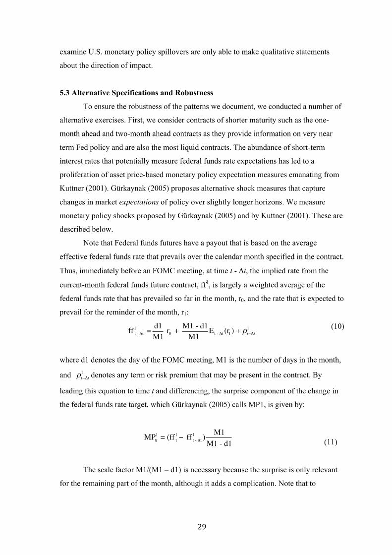
Note that Federal funds futures have a payout that is based on the average

effective federal funds rate that prevails over the calendar month specified in the contract.

Thus, immediately before an FOMC meeting, at time t - Δt, the implied rate from the

current-month federal funds future contract, ff1, is largely a weighted average of the

federal funds rate that has prevailed so far in the month, r0, and the rate that is expected to

prevail for the reminder of the month, r1:

ff1t - Δt =

d1M1

r0 + M1 - d1M1

Et - Δt (r1) + ρt−Δt1

(10)

where d1 denotes the day of the FOMC meeting, M1 is the number of days in the month,

and ρt−Δt1 denotes any term or risk premium that may be present in the contract. By

leading this equation to time t and differencing, the surprise component of the change in

the federal funds rate target, which Gürkaynak (2005) calls MP1, is given by:

MPt1t = (ff1

t − ff1t - Δt )

M1M1 - d1

(11)

The scale factor M1/(M1 – d1) is necessary because the surprise is only relevant

for the remaining part of the month, although it adds a complication. Note that to

30

interpret the above as the surprise change in monetary policy expectations, we need to

assume that the change in the risk premium ρ in this narrow window of time is small in

comparison to the change in expectations itself. For example, for a policy action on the

last day of a month, the change in the term premium is multiplied by thirty amplifying the

noise in the measurement of the surprise. To surmount this problem, Kuttner (2001)

suggests using the next month’s contract (i.e., the month ahead contract in place of the

current month contract) when a policy action takes place in the last week of the month.

Gürkaynak (2005) goes a step further, constructing a measure to capture the

change in the federal funds rate expected to prevail after the next FOMC meeting. Given

the unexpected change in the federal funds rate following the current meeting, MP1t, the

change in the rate expected after the subsequent meeting, MP2t, can be calculated as

follows:

MP2t = M2M2 - d2

(Δff 2t −

d2M2

MP1t ) (12)

where Δff 2t is the change in the federal funds futures contract for the month of the

next FOMC meeting. This is contained in the two-month-ahead contract, as FOMC

meetings are scheduled to take place once every six weeks. As shown Table 1, while

these alternative shocks measures are weakly correlated with our baseline FF5 shock,

they clearly capture different economic information (presumably about very short-term

policy expectations).

To see whether the pattern of results is different for shocks extracted from short

maturity contracts we repeat the estimations using the one-month (MP1) and two-month

(MP2) Fed Funds futures contracts (Table 6). The pattern of results is interesting.

The two monetary policy surprise measures (MP1 and MP2) are included together in

the regression under the assumption that they capture distinct elements of monetary

policy. Interacting our monetary surprise measures with time dummies allows us to

capture the differential effect of monetary policy over three distinct regimes while

allowing our controls to have a regime-invariant effect. Table 6 presents an interesting

pattern of results using these more liquid contracts.

In the pre-crisis period, there appears to be no effect of MP1 on any of our bond flow

measures. In contrast, the coefficient on the MP2 monetary surprise measure is positive

and statistically significant for debt positions and flows (Columns 1 and 2). The MP2

measure based on the two-month Fed Funds Futures contract which captures, in part,

31

revisions in the expected ‘path’ of monetary policy in the conventional policy period. A

positive and statistically significant coefficient therefore suggests that markets interpret a

tightening as a signal that the Fed is feeling sanguine about global market conditions such

that debt positions, flows and valuations in emerging markets increase.

Turning to the equity data, we see that emerging market equity valuations scaled

by destination GDP are inversely related to the MP1 monetary surprise measure, i.e., a

U.S. tightening surprise is correlated with a statistically significant decline in emerging-

market equity valuations (Column 6) consistent with a role for the signaling and portfolio

balance channels. In the pre-crisis period, for all the other capital flow and holdings

measures, monetary surprises extracted from short contracts do not appear to be

significantly correlated with U.S. capital flows to our emerging-market sample countries.

Recall in comparison that the coefficients on the longer five-year Treasury futures

measure (FF5) measure was negative and significant in nearly every specification.

In contrast to the conventional policy period, the QE period displays a somewhat

different pattern for the shocks extracted from the short-duration contracts. The MP1

surprise measure is now positively and statistically significantly correlated with total debt

positions, suggesting that on impact quantitative easing led to a decline in debt flows to

emerging markets (Column 1) consistent with the confidence channel (or a lack thereof).

In contrast, the MP2 measure, associated in large part with revisions in market

participants require risk compensation during this period, is inversely and significantly

correlated with debt positions, valuations and flows (Columns 1-3).

Given that interest rates fell dramatically during this period and the U.S. quickly

entered the ZLB regime, monetary policy surprises extracted from Fed Funds futures

contracts suggest that U.S. investors significantly increased their emerging market debt

and equity holdings during the QE period. Equity positions and valuations are inversely

correlated with the MP1 monetary surprise measure (Columns 4 and 6). However, none

of the equity measures are significantly correlated with the MP2 or path measure of

monetary policy. While it may seem a little puzzling that the equity flow measures do not

exhibit statistical significance, one explanation may be that there is more noise in the

measured flows data during periods of higher volatility.

Similar to the results using five-year Treasury futures surprises, the unwinding, or

taper, period presents a significant shift in the pattern of results. Across both monetary

surprise measures and alternative measures of debt and equity positions, flows and

32

valuations, we see inverse and statistically significant coefficients suggesting that the

period of taper talk and the actual unwinding was associated with significant outflows

from emerging markets. It is also noteworthy that once again the coefficients associated

with the unwinding period are an order of magnitude larger than both the pre-crisis and

the QE periods.

The coefficients on both the MP1 and MP2 measures suggest that the market

interpreted the unwinding of unconditional monetary policy as a signal that normalcy was

being restored to the U.S. economy and, expected monetary tightening in the U.S. both in

the near term and ongoing in the future led to a massive retrenchment from emerging

markets. We assess the magnitude of these effects in Table 5 (Panel B) and see that the

economic magnitudes remain important. For example, during the taper period, the

coefficient on the MP2 change measure on equity positions is -9.2 (Table 6, Column 4).

From Table 1 Panel A, the mean values for the MP2 change, during the taper period is

0.005. Together, these coefficient estimates for reversals in the unwinding period,

the mean- magnitude shocks are correlated on average with monthly position declines of

$435.0M. A one standard deviation tightening (loosening) shock is associated with

monthly position declines (increases) of $1.48B ($607.4M).

We also experimented with longer horizons of the monetary policy shock, for

example at the three and four month Fed Funds futures contract horizons (MP3 and

MP4). The coefficients on these variables did not enter the regressions with consistent

statistical significance. We do not therefore report these results but note that the exercise

established that the relevant monetary surprise measures are MP1 and MP2.

We repeated the estimations with our final monetary surprise measure the

difference in the yield two-year treasury bond on the date of an FOMC meeting. The

principle is the same as the five-year Treasury futures rate—over a very narrow window,

it is reasonable to state that change in the price of the asset reflects a change in the

expectations component of yield i.e., the sum of expected future interest rates, which is

driven by a monetary surprise. The results (not reported) are robust especially for the

taper/unwinding period.19

To examine whether the yield on the two-year bond is capturing expectations

about the path of the short rate over the life of the bond or about changes in risk 19 The results are available upon request.

33

compensation we appeal to Kim and Wright's (2005) decomposition of the bond yield

into expected short rates and term premia. Figure 2 depicts the contribution from the

expected short rate and the term premium to the overall daily changes in the two-year

zero coupon bond yield on FOMC event days. The changes on FOMC dates tend to result

in larger part from changes in the term premium, although the decomposition is also

frequently close to an even contribution.

The dependent variables in the benchmark regressions are scaled by the GDP of

the destination country. We repeated the estimations with the previous period’s holdings

as an alternative scaling variable (Table 7). We also conducted a set of estimations with

destination-country fixed effects. The pattern of results is robust in both cases.20

Finally, we implement our benchmark specification using alternative dates for the

end of the tapering period. To isolate the ''taper tantrum'' from the remainder of the

normalization process, we define the tapering period from May 2013 to December 2013.

This dating increases the magnitude of our estimates for the period of normalization.

Changing the end date of the tapering period to May 2014 leaves our estimates

essentially unchanged from the baseline.

6. Conclusion

This paper examines the implications of unconventional monetary policy and its

continued unwinding for emerging market capital flows and asset prices with an

emphasis on quantifying the magnitude of these effects. We use U.S. Treasury data on

emerging market flows and asset prices alongside Treasury bond futures data to extract a

surprise component of Fed announcements. High frequency identification (HFI) using

Fed Funds futures data allows us to extract the unexpected element of changes in the

market’s expectations of Fed policy.

Using this methodology, we examine the impact of monetary policy surprises

extracted around FOMC meetings on capital flows from the United States to a range of

emerging markets. Panel regression estimates reveal substantial heterogeneity in the

monetary policy shock implications for flows versus asset prices, across asset classes,

and during across the various policy periods. The most robust finding is that the evolution

in overall emerging market debt and equity positions between various policy sub-periods 20 Not reported, but available from the authors.

34

appear to be largely driven by U.S. monetary policy induced valuation changes. In nearly

every specification, the effect of monetary policy shocks on asset values is larger than

that for physical capital flows.

Further, there is an order-of-magnitude difference between the effects of

monetary policy on all types of emerging-market portfolio flows between pre-crisis

conventional monetary policy period, the QE period and the subsequent tapering period.

We detect some significant effects of monetary policy on flows and valuations during the

period of unconventional monetary policy (QE). However, the effects are not consistent

over all dependent variables. In contrast, during the period following the first mentioning

of policy tapering, we uncover a consistent and large effect of monetary policy shocks on

nearly all variables of interest.

A key advantage of extracting the magnitude of the monetary surprises directly

from the Treasury futures data is that we can directly estimate a dollar amount in terms of

US investor position and flow changes to emerging markets controlling for a variety of

push and pull factors. By extracting the magnitude of the monetary surprises we can

quantify the distributional impact of US monetary policy on our emerging-market capital

flow measures consistent with emerging markets’ varied experience across debt and

equity, during the periods of quantitative easing and of its unwinding.

35

6. References

Ahmed, S., Curcuru, S., Warnock, F., and Zlate, A. (2015) "The Two Components of International Capital Flows." Working Paper.

Ahmed, S., and Zlate, A. (2014). Capital flows to emerging market economies: A brave new world? Journal of International Money and Finance, 48, 221-248.

Aizenman, J., Binici, M., & Hutchison, M. M. (2014). The transmission of Federal Reserve tapering news to emerging financial markets. National Bureau of Economic Research Working Paper No. 19980.

Bertaut, C. C., & Judson, R. (2014). Estimating US cross-border securities positions: New data and new methods. FRB International Finance Discussion Paper, (1113).

Bertaut, C. C., & Tryon, R. W. (2007). Monthly estimates of US cross-border securities positions. FRB International Finance Discussion Paper, (910).

Broner, F., Didier, T., Erce, A., & Schmukler, S. L. (2013). Gross capital flows: Dynamics and crises. Journal of Monetary Economics, 60 (1), 113-133.

Burger, J., R. Sengupta, F. Warnock, and V. Warnock (2015). U.S. Investment in Global Bonds: As the Fed Pushes, Some EMEs Pull. Economic Policy.

Calvo, G. A., Leiderman, L., & Reinhart, C. M. (1993). Capital inflows and real exchange rate appreciation in Latin America: The role of external factors. Staff Papers-International Monetary Fund, 108-151.

Chen, J., Mancini Griffoli, T., & Sahay, R. (2014). Spillovers from United States monetary policy on emerging markets: different this time? IMF Working Paper No. 14/240.

Christiano, L. J., Eichenbaum, M., & Evans, C. L. (1999). Monetary policy shocks: What have we learned and to what end? Handbook of Macroeconomics, 1, 65-148.

Curcuru, S. E., Dvorak, T., & Warnock, F. E. (2008). Cross-border returns differentials. Quarterly Journal of Economics 123(4): 1495–1530..

Eichengreen, B., & Gupta, P. (2014). Tapering talk: The impact of expectations of reduced Federal Reserve security purchases on emerging markets. World Bank Policy Research Working Paper, (6754)

Fernandez-Arias, E. (1996). The new wave of private capital inflows: Push or pull? Journal of Development Economics, 48(2), 389-418.

Forbes, K. J., & Rigobon, R. (2002). No contagion, only interdependence: Measuring stock market comovements. The Journal of Finance, 57(5), 2223-2261.

36

Forbes, K. J., & Warnock, F. E. (2012). Capital flow waves: Surges, stops, flight, and retrenchment. Journal of International Economics, 88(2), 235-251.

Fratzscher, M. (2012). Capital flows, push versus pull factors and the global financial crisis. Journal of International Economics, 88(2), 341-356.

Fratzscher, M., Lo Duca, M., & Straub, R. (2013). On the international spillovers of US quantitative easing. European Central Bank, working paper #1557.

Gagnon, J., Raskin, M., Remache, J., and Sack, B. P. (2010). Large-scale asset purchases by the Federal Reserve: did they work?. Federal Reserve Bank of New York Staff Report #441.

Galati, G., Heath, A., & McGuire, P. (2007). Evidence of carry trade activity. BIS Quarterly Review, September.

Ghosh, A. R., Kim, J., Qureshi, M., and Zalduendo, J. (2012). “Surges,” IMF Working Paper WP/12/22.

Gürkaynak, R. S. (2005). Using federal funds futures contracts for monetary policy analysis. FEDS Working Paper No. 2005-29

Gürkaynak, R. S., Sack, B. P., and Swanson, E. T. (2007). Market-based measures of monetary policy expectations. Journal of Business and Economic Statistics, 25(2).

Gürkaynak, R. S., Sack, B., & Swanson, E. (2005). The sensitivity of long-term interest rates to economic news: Evidence and implications for macroeconomic models. American Economic Review, 5 , 425-436.

Gürkaynak, R. S., Sack, B., & Wright, J. H. (2007). The US Treasury yield curve: 1961 to the present. Journal of Monetary Economics, 54(8), 2291-2304.

Joslin, S., Singleton, K. J., & Zhu, H. (2011). A new perspective on Gaussian dynamic term structure models. Review of Financial Studies, 24(3), 926-970.

Karolyi, G. A., & McLaren, K. J. (2016). Racing to the Exits: International Transmissions of Funding Shocks During the Federal Reserve's Taper Experiment. SSRN 2792347.

Kim, S. (2001). International transmission of US monetary policy shocks: Evidence from VARs. Journal of Monetary Economics, 48(2), 339-372.

Kim, D. H. and J. H. Wright, 2005, “An Arbitrage-Free Three-Factor Term Structure Model and the Recent Behavior of Long-Term Yields and Distant-Horizon Forward Rates,” Finance and Economics Discussion Series No. 33, Federal Reserve Board of Governors.

37

Krishnamurthy, A., & Vissing-Jorgensen, A. (2011). The Effects of Quantitative Easing on Interest Rates: Channels and Implications for Policy, Brookings Papers on Economic Activity, pp. 215-287.

Kuttner, K. N. (2001). Monetary policy surprises and interest rates: Evidence from the Fed funds futures market. Journal of Monetary Economics, 47(3), 523-544.

Lim, J. J., Mohapatra, S., & Stocker, M. (2014). Tinker, taper, QE, bye? the effect of quantitative easing on financial flows to developing countries. World Bank Policy Research Working Paper, (6820)

Milesi-Ferretti, G., & Tille, C. (2011). The great retrenchment: International capital flows during the global financial crisis. Economic Policy, 26(66), 289-346.

Montiel, P., & Reinhart, C. M. (1999). Do capital controls and macroeconomic policies influence the volume and composition of capital flows? Evidence from the 1990s. Journal of International Money and Finance, 18(4), 619-635.

Moore, J., Nam, S., Suh, M., & Tepper, A. (2013). Estimating the Impacts of US LSAP's on Emerging Market Economies' Local Currency Bond Markets. Federal Reserve Bank of New York Staff Report #595.

Neely, C. J. (2010). The large scale asset purchases had large international effects (pp. 1-45). Federal Reserve Bank of St. Louis, Research Division.

Obstfeld, M., & Rogoff, K. (1995). Exchange Rate Dynamics Redux. Journal of Political Economy, 103, 624–660.

Passari, E., & Rey, H. (2015). Financial Flows and the International Monetary System (No. w21172). National Bureau of Economic Research.

Rey, H. (2015). Dilemma not trilemma: the global financial cycle and monetary policy independence. National Bureau of Economic Research Working Paper No. 21162.

Rogers, J. H., Scotti, C., & Wright, J. H. (2014). Evaluating asset-market effects of unconventional monetary policy: a multi-country review. Economic Policy, 29(80), 749-799.

Taylor, M. P., & Sarno, L. (1997). Capital flows to developing countries: Long-and short-term determinants. The World Bank Economic Review, 11(3), 451-470.

Tille, C., & Van Wincoop, E. (2010). International capital flows. Journal of International Economics, 80(2), 157-175.

Warnock, F. E., & Warnock, V. C. (2009). International capital flows and US interest rates. Journal of International Money and Finance, 28(6), 903-919.

38

Appendix 1: Description of Variables Variable Description Source Bond/equity positions

Sum of bond/equity flows, valuation changes and gap

Bertaut and Tryon (2007), Bertaut and Judson (2009)

Total positions Equity positions plus bond positions

Bertaut and Tryon (2007), Bertaut and Judson (2009)

Bond/equity flows TICS Reported transactions plus repayment of principal on asset-backed securities and stock swaps from mergers and acquisitions

Bertaut and Tryon (2007), Bertaut and Judson (2009)

Total flows Equity flows plus bond flows Bertaut and Tryon (2007), Bertaut and Judson (2009)

Bond/equity valuation changes

Cumulative change in the value of time t holdings between time t and t+n as measured by a weighted average of local currency and dollar-denominated asset returns

Bertaut and Tryon (2007), Bertaut and Judson (2009)

Bond/equity flows (% of holdings)

Ratio of current flows (t) to previous period holdings (t-1)

Bertaut and Tryon (2007), Bertaut and Judson (2009) and author’s calculations

Bond/equity gap Difference between the year-end annual survey holdings data and the cumulation-implied holdings, distributed over between-survey months proportional to the size of monthly flows

Bertaut and Tryon (2007), Bertaut and Judson (2009)

VIX Implied volatility of S&P 500 index options

FRED database

Treasury Futures Rate

Implied yield from the five-year Treasury futures price

Bloomberg

Fed Funds rate Federal reserve target interest rate

FRED database

Change in Fed Funds rate

Monthly first difference of the Fed Funds rate

FRED database

Ted spread 3-month LIBOR minus 3-month T-bill interest rate

FRED database

S&P annual return Annual return on the S&P index Standard and Poor’s Policy rate Domestic (EM) central bank

target interest rate Datastream

Change in policy rate Monthly first difference of domestic policy rate

Datastream

EMBI annual return Year-on-year growth of MSCI total return index

Datastream

MSCI annual return Year-on-year growth of MSCI total return index

Datastream

39

Figure 1: Five-Year Treasury Futures Yield Changes on FOMC Event Dates

Figure 1 depicts daily changes in the implied yield from five-year Treasury futures contracts on FOMC dates aggregated at the monthly level. Red lines indicate major monetary policy events starting with the advent of quantitative easing. Figure 2: Decomposition of the two year zero coupon bond yield

Figure 2 depicts the decomposition of the two-year Treasury bond yield into an expected average short rate (Y(eh)) and a term premium (YTP) using the affine-term structure model in Kim and Wright (2005).

QE1

QE2

Twis

tQ

E3 TT1

TT2

-.4-.2

0.2

Five

Yea

r Fut

ures

Yie

ld C

hang

e

1994

m1

1995

m1

1996

m1

1997

m1

1998

m1

1999

m1

2000

m1

2001

m1

2002

m1

2003

m1

2004

m1

2005

m1

2006

m1

2007

m1

2008

m1

2009

m1

2010

m1

2011

m1

2012

m1

2013

m1

2014

m1

2015

m1

2016

m1

Date

-0.4

-0.3

-0.2

-0.1

0

0.1

0.2

0.3

1/31

/06

6/30

/06

11/3

0/06

4/

30/0

7 9/

30/0

7 2/

29/0

8 7/

31/0

8 12

/31/

08

5/31

/09

10/3

1/09

3/

31/1

0 8/

31/1

0 1/

31/1

1 6/

30/1

1 11

/30/

11

4/30

/12

9/30

/12

2/28

/13

7/31

/13

12/3

1/13

5/

31/1

4 10

/31/

14

3/31

/15

8/31

/15

1/31

/16

ΔYTP ΔY(eh)

40

41

42

43

44

Panel A: Using Five-year Treasury Bond Futures (FF5)

(1) (2) (3) (4) (5) (6)µ µ-σ µ+σ µ µ-σ µ+σ

Bond positions -49.60 234.95 -334.16Debt flows -24.65 116.77 -166.08Debt valuations 12.43 79.33 -54.46 -29.85 141.39 -201.09Equity positions 138.46 883.31 -606.39 -130.24 616.93 -877.41

Equity flows -46.93 222.29 -316.15Equity valuations 118.30 754.72 -518.12 -95.34 451.62 -642.30Exchange rate 0.04 0.28 -0.19 -0.10 0.49 -0.69

Panel B: Using Fed Funds Futures (MP1 and MP2)

(1) (2) (3) (4) (5) (6)µ µ-σ µ+σ µ µ-σ µ+σ

Bond positions -14.62 -121.84 92.59 39.99 217.74 -137.75Debt flowsDebt volume 21.27 115.82 -73.28Debt valuations 16.03 87.30 -55.23Equity positions 79.47 662.21 -503.28Equity flowsEquity volumeEquity valuations 90.54 754.50 -573.42

(1) (2) (3) (4) (5) (6)µ µ-σ µ+σ µ µ-σ µ+σ

Bond positions 11.51 486.62 -463.60 -223.33 311.82 -758.49Debt flowsDebt volume 10.91 461.09 -439.28 -141.44 197.48 -480.36Debt valuations 1.56 66.08 -62.95 -119.89 167.39 -407.17Equity positions 23.93 1011.92 -964.05 -435.00 607.35 -1477.34Equity flowsEquity volume 4.96 209.59 -199.68Equity valuations 20.14 851.61 -811.32 -471.95 658.94 -1602.85

Table 5 presents the response of monthly capital flows and valuation changes to the monetary policy shocks evaluated at the mean as well as for a one standard deviation shock from the mean. The effect is calculated in the following manner. Let GDPt be the average GDP of the sample countries in the two periods of interest, QE and normalization. Let βi,t be the coefficient on monetary policy shock measure i during period of interest t (i = MP1, MP2, FF5) from Table 4. Let µi,t be the average monetary policy shock during the period of interest t. Let σi,t be a one standard deviation shock above or below the mean during subsample t, µi,t. Let Qi,t be the average economic impact of monetary policy shock i on the flow measure of interest during sample period t. Let Qi,t(+,-) be the average economic impact of a monetary policy shock i that is one standard deviation above (+) or below (-) the mean on the flow measure of interest during sample period t. Then panel A, columns 1, 2 and 3 contain: QFF5,QE = GDPFF5,QE *βFF5,QE*µFF5,QE, QFF5,QE (-) = GDPFF5,QE *βFF5,QE*(µFF5,QE - σFF5,QE) QFF5,QE (+) = GDPFF5,QE *βFF5,QE*(µFF5,QE + σFF5,QE), respectively. Empty cells indicate a statistically insignificant regression coefficient on capital flow measure of interest in Table 4 (Panel A) or Table 6 (Panel B). All flow values are expression in USD Millions. Exchange rate changes are expressed in percentage points. (-) indicates outflow.

QE period Taper/Unwinding period

Table 5. Economic Significance: The Quantitative Impact (Q) of US Monetary Policy on Emerging Market Capital Flows.

Empty cells indicate a statistically insignificant coefficient for capital flow measure of interest in Table 4. All flow values in USD Million; (-) indicates outflows; (+) indicates inflows.

QE periodMP1 shocks MP2 shocks

Taper/Unwinding periodMP1 shocks MP2 shocks

45

46

47