taming subgraph isomorphism for rdf query processing … · · 2015-06-08taming subgraph...
TRANSCRIPT
Taming Subgraph Isomorphism for RDF Query Processing
Jinha Kim †#
[email protected] Shin †
[email protected] Han †∗
Sungpack Hong # Hassan Chafi #
{sungpack.hong, hassan.chafi}@oracle.com†POSTECH, South Korea #Oracle Labs, USA
ABSTRACTRDF data are used to model knowledge in various areas such as lifesciences, Semantic Web, bioinformatics, and social graphs. Thesize of real RDF data reaches billions of triples. This calls for aframework for efficiently processing RDF data. The core functionof processing RDF data is subgraph pattern matching. There havebeen two completely different directions for supporting efficientsubgraph pattern matching. One direction is to develop specializedRDF query processing engines exploiting the properties of RDFdata for the last decade, while the other direction is to develop effi-cient subgraph isomorphism algorithms for general, labeled graphsfor over 30 years. Although both directions have a similar goal(i.e., finding subgraphs in data graphs for a given query graph),they have been independently researched without clear reason. Weargue that a subgraph isomorphism algorithm can be easily modi-fied to handle the graph homomorphism, which is the RDF patternmatching semantics, by just removing the injectivity constraint. Inthis paper, based on the state-of-the-art subgraph isomorphism al-gorithm, we propose an in-memory solution, TurboHOM++, whichis tamed for the RDF processing, and we compare it with the repre-sentative RDF processing engines for several RDF benchmarks in aserver machine where billions of triples can be loaded in memory.In order to speed up TurboHOM++, we also provide a simple yeteffective transformation and a series of optimization techniques.Extensive experiments using several RDF benchmarks show thatTurboHOM++ consistently and significantly outperforms the repre-sentative RDF engines. Specifically, TurboHOM++ outperforms itscompetitors by up to five orders of magnitude.
1. INTRODUCTIONThe Resource Description Framework (RDF) is a standard for
representing knowledge on the web. It is primarily designed forbuilding the Semantic web and has been widely adopted in databaseand data mining communities. RDF models a fact as a triple whichconsists of a subject (S), a predicate (P), and an object (O). Dueto its simple structure, many practitioners materialize their data in
∗corresponding author
This work is licensed under the Creative Commons Attribution-NonCommercial-NoDerivs 3.0 Unported License. To view a copy of this li-cense, visit http://creativecommons.org/licenses/by-nc-nd/3.0/. Obtain per-mission prior to any use beyond those covered by the license. Contactcopyright holder by emailing [email protected]. Articles from this volumewere invited to present their results at the 41st International Conference onVery Large Data Bases, August 31st - September 4th 2015, Kohala Coast,Hawaii.Proceedings of the VLDB Endowment, Vol. 8, No. 11Copyright 2015 VLDB Endowment 2150-8097/15/07.
an RDF format. For example, RDF datasets are now pervasive invarious areas including life sciences, bioinformatics, and social net-works. The size of real RDF data reaches billions of triples. Suchbillion-scale RDF data are fully loaded in main memory of today’sserver machine (The cost of a 1TB machine is less than $40,000).
The SPARQL query language is a standard language for query-ing RDF data in a declarative fashion. Its core function is subgraphpattern matching, which corresponds to finding all graph homo-morphisms in the data graph for a query graph [19].
In recent years, there have been significant efforts to speed up theprocessing of SPARQL queries by developing novel RDF queryprocessing engines. Many engines [1, 18, 19, 25, 26, 29] modelRDF data as tabular structures and process SPARQL queries usingspecialized join methods. For example, RDF-3X [19] treats RDFdata as an edge table, EDGE(S,P,O), and materializes six differ-ent orderings for this table, so that it can support many SPARQLqueries just by using merge based join. Note that this approachis efficient for both disk-based and in-memory environments sincemerge join exploits only sequential scans. Some engines [2, 30, 35]treat RDF data as graphs (or matrices) and develop specializedgraph processing methods for processing SPARQL queries. Forexample, gStore [35] uses specialized index structures to processSPARQL queries. Note that these index structures are based ongCode [34], which was originally proposed for graph indexing.
Subgraph isomorphism, on the other hand, has been studied sincethe 1970s. The representative algorithms are VF2 [20], QuickSI[21], GraphQL [11], GADDI [32], SPATH [33], and TurboISO [9].In order to speed up performance, these algorithms exploit goodmatching orders and effective pruning rules. A recent study [14]shows that good subgraph isomorphism algorithms significantlyoutperform graph indexing based ones. However, all of these al-gorithms use only small graphs in their experiments, and thus, itstill remains unclear whether these algorithms can show good per-formance for billion-scale graphs such as RDF data.
Although subgraph isomorphism processing and RDF query pro-cessing have similar goals (i.e., finding subgraphs in data graphsfor a given query graph), they have two inexplicably different di-rections. A subgraph isomorphism algorithm can be easily modi-fied to handle the graph homomorphism, which is the RDF patternmatching semantics, just by removing the injectivity constraint.
In this paper, based on the state-of-the-art subgraph isomorphismalgorithm [9], we propose an in-memory solution, TurboHOM++,which is tamed for the RDF processing, and we compare it withthe representative RDF processing engines for several RDF bench-marks in a server machine where billions of triples can be loadedin memory. We believe that this approach opens a new directionfor RDF processing so that both traditional directions can merge orbenefit from each other.
1238
By transforming RDF graphs into labeled graphs, we can ap-ply subgraph homomorphism methods to RDF query processing.Extensive experiments using several benchmarks show that a di-rect modification of TurboISO outperforms the RDF processing en-gines for queries which require a small amount of graph explo-ration. However, for some queries which require a large amountof graph exploration, the direct modification is slower than someof its competitors. This poses an important research question: “Isthis phenomenon due to inherent limitations of the graph homo-morphism (subgraph isomorphism) algorithm?” Our profile resultsshow that two major subtasks of TurboISO — 1) exploring candi-date subgraphs inExploreCandidateRegion and 2) enumeratingsolutions based on candidate regions in SubgraphSearch — re-quire performance improvement. TurboHOM++ resolves such per-formance hurdles by proposing the type-aware transformation andtailored optimization techniques.
First, in order to speed upExploreCandidateRegion, we pro-pose a novel transformation (Section 4.1), called type-aware trans-formation, which is simple yet effective in processing SPARQLqueries. In type-aware transformation, by embedding the types ofan entity (i.e., a subject or object) into a vertex label set, we caneliminate corresponding query vertices/edges from a query graph.With type-aware transformation, the query graph size decreases, itstopology becomes simpler than the original query, and thus, thistransformation improves performance accordingly by reducing theamount of graph exploration.
In order to optimize performance in depth, in both Explore-CandidateRegion and SubgraphSearch, we propose a seriesof optimization techniques (Section 4.3), each of which contributesto performance improvement significantly for such slow queries.In addition, we explain how TurboHOM++ is extended to support1) general SPARQL features such as OPTIONAL, and FILTER,and 2) parallel execution for TurboHOM++ in a non-uniform mem-ory access (NUMA) architecture [15, 16]. These general featuresare necessary to execute comprehensive benchmarks such as BerlinSPARQL benchmark (BSBM) [3]. Note also that, when the RDFdata size grows large, we have to rely on the NUMA architecture.
Extensive experiments using several representative benchmarksshow that TurboHOM++ consistently and significantly outperformsall its competitors for all queries tested. Specifically, our methodoutperforms the competitors by up to five orders of magnitude withonly a single thread. This indicates that a subgraph isomorphismalgorithm tamed for RDF processing can serve as an in-memoryRDF accelerator on top of a commercial RDF engine for real-timeRDF query processing.
Our contributions are as follows. 1) We provide the first directcomparison between RDF engines and the state-of-the-art subgraphisomorphism method tamed for RDF processing, TurboHOM++, thro-ugh extensive experiments and analyze experimental results in depth.2) In order to simplify a query graph, we propose a novel trans-formation method called type-aware transformation, which con-tributes to boosting query performance. 3) In order to speed upquery performance further, we propose a series of performanceoptimizations as well as NUMA-aware parallelism for fast RDFquery processing. 4) Extensive experiments using several bench-marks show that the optimized subgraph isomorphism method con-sistently and significantly outperforms representative RDF queryprocessing engines.
The rest of the paper is organized as follows. Section 2 de-scribes the subgraph isomorphism, its state-of-the-art algorithms,TurboISO, and their modification for the graph homomorphism. Sec-tion 3 presents how a direct modification of TurboISO, TurboHOM,handles the SPARQL pattern matching. Section 4 describes how we
obtain TurboHOM++ from TurboHOM using the type-aware transfor-mation and optimizations for the efficient SPARQL pattern match-ing. Section 5 reviews the related work. Section 6 presents the ex-perimental result. Finally, Section 7 presents our conclusion. Notethat due to the space limit, please refer [13] for how TurboHOM++handle OPTIONAL, UNION, FILTER keywords, and parallelize.
2. PRELIMINARY
2.1 Subgraph Isomorphism and RDF PatternMatching Semantic
Suppose that a labeled graph is defined as g(V,E, L), where Vis a set of vertices,E(⊆ V ×V ) is a set of edges, andL is a labelingfunction which maps from a vertex or an edge to the correspondinglabel set or label, respectively. Then, the subgraph isomorphism isdefined as follows.
Definition 1. [14] Given a query graph q(V,E, L) and a datagraph g(V ′, E′, L′), a subgraph isomorphism is an injective func-tion M : V → V ′ such that 1) ∀v ∈ V,L(v) ⊆ L′(M(v)) and 2)∀(u, v) ∈ E, (M(u),M(v)) ∈ E′ andL(u, v) = L′(M(u),M(v)).
If a query vertex, u, has a blank label set (or does not spec-ify vertex label equivalently), it can match any data vertex. Here,L(u) = ∅, and thus, the subset condition, L(u) ⊆ L′(M(u)), isalways satisfied. Similarly, if a query edge (u, v) has a blank label,it can match any data edge by generalizing the equality conditionL(u, v) = L′(M(u),M(v)) to L(u, v) ⊆ L′(M(u),M(v)).
The graph homomorphism [6] is easily obtained from the sub-graph isomorphism by just removing the injective constraint on Min Definition 1. Even though the RDF pattern matching semanticsis based on the graph homomorphism, to answer SPARQL querieswhich have variables on predicates, a mapping from a query edgeto an edge label is also required. We call such graph homomor-phism the e(xtended)-graph homomorphism and present a formaldefinition for it as follows.
Definition 2. Given a query graph q(V,E, L) and a data graphg(V ′, E′, L′), an e(xtended)-graph homomorphism is a pair of twomapping functions, a query vertex to data vertex function Mv :V → V ′ such that 1) ∀v ∈ V,L(v) ⊆ L′(Mv(v)) and 2) ∀(u, v) ∈E, (Mv(u),Mv(v)) ∈ E′, and L(u, v) = L′(Mv(u),Mv(v)),and a query edge to edge label function Me : V × V → L suchthat ∀(u, v) ∈ E,Me(u, v) = L′(Mv(u),Mv(v)).
The subgraph isomorphism problem (resp. the e-graph homo-morphism problem) is to find all distinct subgraph isomorphisms(resp. e-graph homomorphisms) of a query graph in a data graph.
Figure 1 shows a query q1 and a data graph g1. In q1, _ means ablank vertex label set or blank edge label. In the subgraph isomor-phism, there is only one solution – M1 = {(u0, v0), (u1, v1), (u2,v2), (u3, v3), (u4, v4)}. In the e-graph homomorphism, there arethree solutions – M1
v = M1, M1e = {((u0, u1), a), ((u0, u4), b),
((u2, u1), a), ((u2, u3), a), ((u3, u4), c)}, M2v = {(u0, v2), (u1,
v3), (u2, v2), (u3, v3), (u4, v5)},M2e =M1
e , andM3v = {(u0, v2),
(u1, v1), (u2, v2), (u3, v3), (u4, v5)}, M3e =M1
e .
2.2 TurboISO
In this subsection, we introduce the state-of-the art subgraph iso-morphism solution, TurboISO[9], and its modification for the e-graph homomorphism. Although we only describe the modifica-tion of TurboISO for the e-graph homomorphism, such modificationis applicable to other subgraph isomorphism algorithms including
1239

a
b
_
{A}
{A,D}
{B}
{B}{C}
{C,E}{A}
_
{A}
{B}{C}
a
a
a
a
a
b
b
e
u0
u1
u2
u3
u4
v0
v1
v2
v3v4
c
v4
(a) query graph q1.
a
b
_
{A}
{A,D}
{B}
{B}{C}
{C,E}{A}
_
{A}
{B}{C}
a
a
a
a
a
b
b
c
u0
u1
u2
u3
u4
v0
v1
v2
v3v4
c
v5
(b) data graph g1.
Figure 1: Example of subgraph isomorphism and e-graph ho-momorphism.
VF2 [20], QuickSI [21], GraphQL [11], GADDI [32], and SPATH[33], since all of the subgraph algorithms mentioned are instancesof a generic subgraph isomorphism framework [14].
TurboISO presents an effective method for the notorious match-ing order problem from which all the previous subgraph isomor-phism algorithms have suffered [14]. Figure 2 illustrates an exam-ple of the matching order problem, where q2 is the query graph,and g2 is the data graph1. Note that this example query resultsin no answers. However, the time to finish this query can differdrastically by how one chooses the matching order, as it leads todifferent number of comparisons. For instance, a matching order< u0, u2, u1, u3 > requires 1+10000 ∗ 10 ∗ 5 comparisons whilea different matching order < u0, u3, u1, u2 > requires only 1 + 5* 10 comparisons.
query graph: q
Xu1
A
u0
u2
Y
14 36
X Y
v0 A
X. . .v1 v11
Zu3
ZZ . . .Y. . .
10Xs 10000Ys 5Zs
v12 v10011 v10012 v10016
(a) query graph q2.
query graph: q
Xu1
A
u0
u2
Y
15 36
X Y
v0 A
X. . .v1 v11
Zu3
ZZ . . .Y. . .
10Xs 10000Ys 5Zs
v12 v10011 v10012 v10016
Z Z X X. . .. . .
CR(v0)
(b) data graph g2.
Figure 2: Example of showing the matching order problem.
TurboISO solves the matching order problem with candidate re-gion exploration, a technique that accurately estimates the num-ber of candidate vertices for a given query path [9]. In particu-lar, TurboISO first identifies candidate data subgraphs (i.e., candi-date regions) from the starting vertices (e.g. the shaded area inFigure 2b), then explores each region by performing a depth-firstsearch, which allows almost exact selectivity for each query path.
Algorithm 1 outlines the overall procedure of TurboISO in de-tail. First, if a query graph has only one vertex u and no edge,it is sufficient to retrieve all data vertices which have u’s labels(= V (g)L(u)) and to find a subgraph isomorphism for each of them(lines 2–4). Otherwise, it selects the starting query vertex from thequery graph (line 6). Then, it transforms the query graph into itscorresponding query tree (line 7). After getting the query tree, foreach data vertex that contains the vertex label of the starting queryvertex, the candidate region is obtained by exploring the data graph1For simplicity, we omit the edge labels and allow only one vertexlabel in the data graph.
(lines 9). If the candidate region is not empty, its matching orderis determined (line 11). The data vertex, vs, is mapped to the firstquery vertex us by assigning M(us) = vs and F (vs) = truewhere F : V → boolean is a function which checks whethera data vertex is mapped or not (line 12). Then, the remainingsubgraph matching is conducted (line 13). Lastly, the mapping(us, vs) is restored by removing the mapping for us and assign-ing F (vs) = false (line 14).
Algorithm 1 TurboISO(g(V,E, L), q(V ′, E′, L′))Require: q: query graph, g: data graphEnsure: all subgraph isomorphisms from q to g.1: if V (q) = {u} and E = φ then2: for each v ∈ V (g)L(u) do3: report M = {(u, v)}4: end for5: else6: us ← ChooseStartQueryV ertex(q, g)7: q′ ←WriteQueryTree(q, us)8: for each vs ∈ {v|v ∈ V,L(us) ⊆ L(v)} do9: CR← ExploreCandidateRegion(us, vs)
10: if CR is not empty then11: order ← DetermineMatchingOrder(q′, CR)12: UpdateState(M,F, us, vs)13: SubgraphSearch(q, q′, g, CR, order, 1)14: RestoreState(M,F, us, vs)15: end if16: end for17: end if
ChooseStartQueryVertex. ChooseStartQueryV ertex triesto pick the starting query vertex which has the least number ofcandidate regions. First, as a rough estimation, the query ver-tices are ranked by their scores. The score of a query vertex uis rank(u) = freq(g,L(u))
deg(u), where freq(g, L(u)) is the number of
data vertices that have u’s vertex labels. The score function preferslower frequencies and higher degrees. After obtaining the top-k least-scored query vertices, the number of candidate regions ismore accurately estimated for each of them by using the degree fil-ter and the neighborhood label frequency (NLF) filter. The degreefilter qualifies the data vertices which have equal or higher degreethan their corresponding query vertices. The NLF filter qualifiesthe data vertices which have equal or larger number of neighborsfor all distinct labels of the query vertex. In Figure 2, for example,u0 becomes the starting query vertex since it has the least numberof candidate regions (= 1).
WriteQueryTree. Next,WriteQueryTree transforms the querygraph to the query tree. From the starting query vertex obtained byChooseStartQueryV ertex, a breath-first tree traversal is con-ducted. Every non-tree edge (u, v) of the query graph also is recordedin the corresponding query tree. For example, when u0 is thestarting query vertex, the non-tree edges of q2’s query tree are(u1, u2),(u1, u3), and (u2, u3).
ExploreCandidateRegion. Using the query tree and the startingquery vertex, ExploreCandidateRegion collects the candidateregions. A candidate region is obtained by exploring the data graphfrom the starting query vertex in a depth-first manner following thetopology of the query tree. During the exploration, the injectivityconstraint should be enforced. The shaded area of Figure 2b is thecandidate region CR(v0) based on q2’s query tree. Note that thecandidate region expansion is conducted only after the current datavertex satisfies the constraints of the degree filter and the NLF filter.
1240
DetermineMatchingOrder. After obtaining the candidate re-gions for a starting data vertex, the matching order is determined foreach candidate region. Using the candidate region, Determine-MatchingOrder can accurately estimate the number of candidatevertices for each query path. Then, it orders all query paths in thequery tree by the number of candidate vertices. For example, fromCR(v0), the ordered list of query paths is [u0.u3, u0.u1, u0.u2].Thus, we can easily see that < u0, u3, u1, u2 > is the best match-ing order based on this ordered list.
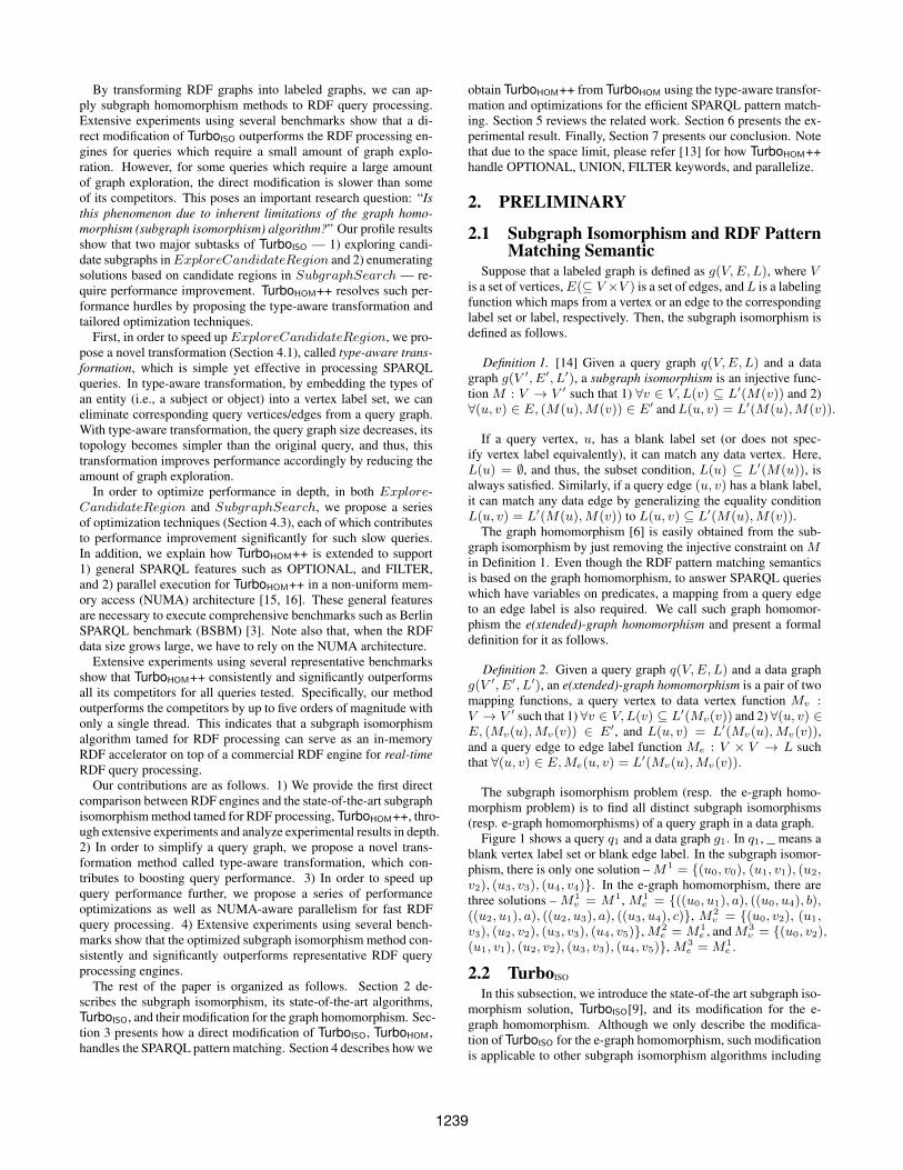
SubgraphSearch. Exploiting the data structures obtained fromthe previous steps, SubgraphSearch (Algorithm 2) enumeratesall distinct subgraph isomorphisms. It first determines the currentquery vertex u from a given matching order order (line 1). Then,it obtains a set of data vertices, CR from a candidate region CR(line 2). CR(u, v) represents the candidate vertices of a query ver-tex u which are the children of v in CR, and P (q′, u) is the parentof u in a query tree q′. For each candidate data vertex v, if v hasalready been mapped, the current solution is rejected since it vio-lates the injectivity constraint of the subgraph isomorphism (lines4–6). Next, by calling IsJoinable, if the query vertex u of thecurrent data vertex v has non-tree edges, the existence of the corre-sponding edges are checked in the data graph (line 7). For example,given CR(v0) and the matching order < u0, u3, u1, u2 >, whenmaking the embedding for u1, we must check whether there is anedge from M(u1) to M(u3). If the IsJoinable test is passed,the mapping information is updated by assigning M(u) = v andF (v) = true (line 8). After updating the mapping, if all queryvertices are mapped, a subgraph isomorphism M is reported (lines9–10). Otherwise, further subgraph search is conducted (line 12).Finally, all changes done by UpdateState are restored (line 14).
Algorithm 2 SubgraphSearch(q, q′, g, CR, order, dc)1: u← order[dc]2: CR ← CR(u,M(P (q′, u)))3: for each v ∈ CR such that v is not yet matched do4: if F (v) = true then5: continue6: end if7: if IsJoinable(q, g,M, u, v, . . . ) then8: UpdateState(M,F, u, v)9: if |M | = V (q) then
10: report M11: else12: SubgraphSearch(q, q′, g, CR, order, dc + 1)13: end if14: RestoreState(M,F, u, v)15: end if16: end for
Modifying TurboISO for e-Graph Homomorphism. We firstexplain how the generic subgraph isomorphism algorithm [14] caneasily handle graph homomorphism. The generic subgraph isomor-phism algorithm is implemented as a backtrack algorithm, wherewe find solutions by incrementing partial solutions or abandon-ing them when it is determined that they cannot be completed.Here, given a query graph q and its matching order (uσ(1), uσ(2),..., uσ(|V (q)|)), a solution is modeled as a vector ~v = (M(uσ(1)),M(uσ(2)), ..., M(uσ(|V (q)|))) where each element in ~v is a datavertex for the corresponding query vertex in the matching order. Ateach step in the backtrack algorithm, if a partial solution is given,we extend it by adding every possible candidate data vertex at theend. Here, any candidate data vertex that does not satisfy the fol-lowing three conditions must be pruned.
1) ∀ui ∈ V (q), L(ui) ⊆ L(M(ui))
2) ∀(ui, uj) ∈ E(q), (M(ui),M(uj)) ∈ E(g) andL(ui, uj) =L(M(ui),M(uj))
3) M(ui) 6=M(uj) if ui 6= uj
Note that the third condition ensures the injective condition, guar-anteeing that no duplicate data vertex exists in each solution vector.Thus, by just disabling the third condition, the generic subgraphisomorphism algorithm finds all possible homomorphisms.
Now, we describe how to disable the third condition in TurboISO,which is an instance of the generic subgraph isomorphism algo-rithm. TurboISO uses pruning rules by applying filters in Explore-CandidateRegion and SubgraphSearch. First, the degree filterand the NLF filter should be modified since a data vertex can bemapped to multiple query vertices. The degree filter qualifies datavertices which have an equal number or more neighbors than dis-tinct labels of their corresponding query vertices. The NLF filterqualifies data vertices which have at least one neighbor for all dis-tinct labels of their corresponding query vertices. Second, lines4–6 of SubgraphSearch ensuring the third condition should beremoved in order to disable the injectivity test. As we see here,with minimal modification to TurboISO, it can easily support graphhomomorphism.
In order to make TurboISO handle the e-graph homomorphism,the query edge to edge label mapping, Me, should be addition-ally added in SubgraphSearch. For this, UpdateState assignsMe(P (q′, u), u) = L(Mv(P (q′, u)),Mv(u)) , andRestoreStateremoves such mapping. From here on, let us denote TurboISO mod-ified for the e-graph homomorphism as TurboHOM.
3. RDF QUERY PROCESSING BY E-GRAPHHOMOMORPHISM
In this section, we discuss how RDF datasets can be naturallyviewed as graphs (Section 3.1), and thus how an RDF dataset canbe directly transformed into a corresponding labeled graph (Sec-tion 3.2). After such a transformation, henceforth, the subgraphisomorphism algorithms modified for the e-graph homomorphismsuch as TurboHOM can be applied for processing SPARQL queries.
3.1 RDF as GraphAn RDF dataset is a collection of triples each of which consists
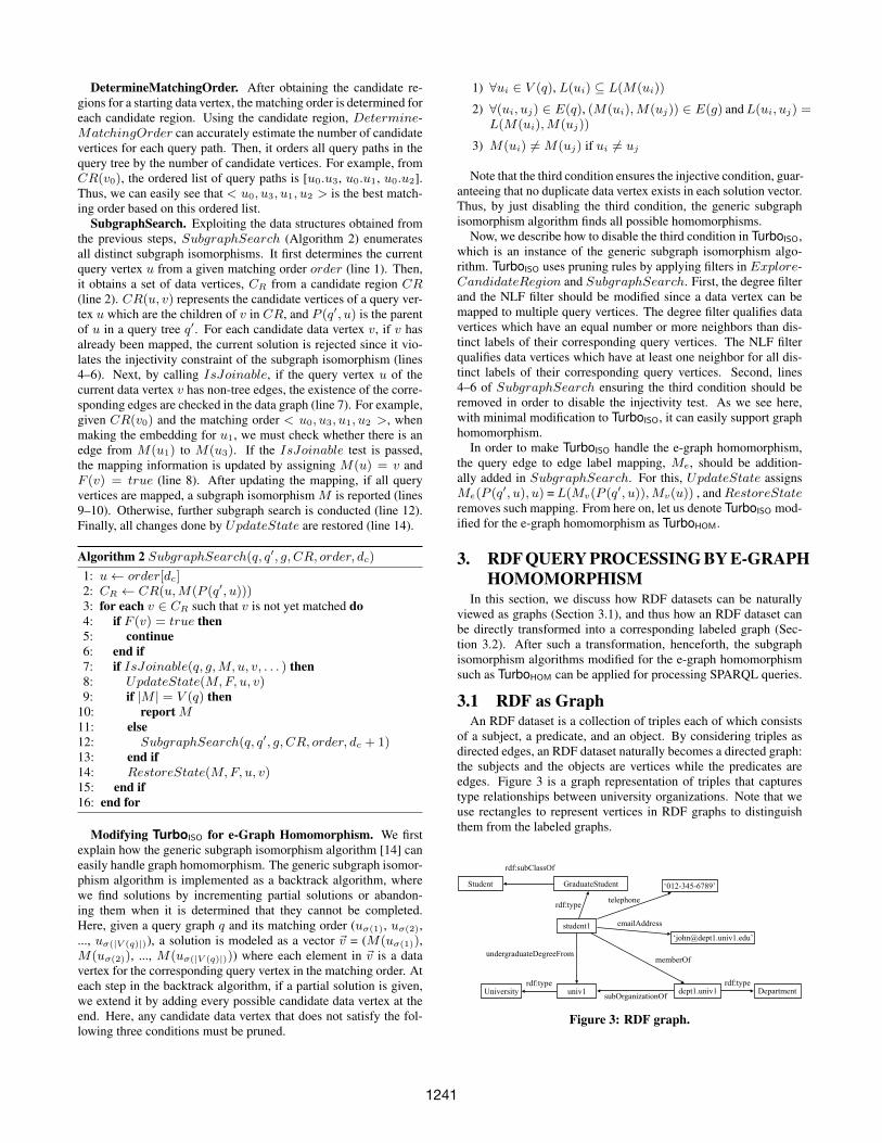
of a subject, a predicate, and an object. By considering triples asdirected edges, an RDF dataset naturally becomes a directed graph:the subjects and the objects are vertices while the predicates areedges. Figure 3 is a graph representation of triples that capturestype relationships between university organizations. Note that weuse rectangles to represent vertices in RDF graphs to distinguishthem from the labeled graphs.
student1
rdf:type
GraduateStudent
univ1rdf:type
University
undergraduateDegreeFrom
dept1.univ1rdf:type
Department
memberOf
subOrganizationOf
‘012-345-6789’
telephone
emailAddress
Student
rdf:subClassOf
Figure 3: RDF graph.
1241
3.2 Direct TransformationTo apply subgraph isomorphism algorithms modified for e-graph
homomorphism (e.g. TurboHOM) for RDF query processing, RDFgraphs have to be transformed into labeled graphs first.
The most basic way to transform RDF graphs is (1) to map sub-jects and objects to vertex IDs and (2) to map predicates to edge la-bels. We call such transformation the direct transformation becausethe topology of the RDF graph is kept in the labeled graph after thetransformation. The vertex label function L(v)(v ∈ V (g)) is theidentity function (i.e. L(v) = {v}).
Figure 4 shows the result of the direct transformation of Figure 3– Figures 4a, 4b, and 4c are the vertex mapping table , the edgelabel mapping table, and the transformed graph, respectively.
Subject/Object VertexGraduateStudent v0
Student v1University v2
Department v3student1 v4
univ1 v5dept1.univ1 v6
‘012-345-6789’ v7‘[email protected]’ v8
(a) vertex mapping table.
Predicate Edge Labelrdf:type a
rdf:subClassOf bundergradDegreeFrom c
memberOf dsubOrganizationOf e
telephone femailAddress g
(b) edge label mapping table.
a
a
c
a
d
e
fg
bv1 v0
v2
v4
v5
v7
v8
v6 v3
{v1} {v0}
{v2} {v5}
{v4}
{v7}
{v8}
{v6} {v3}
(c) graph.
Figure 4: Direct transformation of RDF graph (Vertex labelfunction L(v) = {v}).
A query graph is obtained from a SPARQL query. A query vertexmay hold the vertex label which corresponds to the subject or objectspecified in the SPARQL query. If the query vertex corresponds toa variable, the vertex label is left blank. For example, the SPARQLquery of Figure 5a is transformed into the query graph of Figure 5b.Here the query vertex u0, which corresponds to Student, holdsthe vertex label {v1}; To the contrary, the query vertex u3, whichcorresponds to the variable X , has blank (_) as the vertex label.Similarly, a query edge may hold the edge label which correspondsto the predicate. For example, the edge label of (u3, u4) is c as theedge corresponds to the undergradDegreeFrom predicate.
SELECT ?X, ?Y, ?Z WHERE{?X rdf:type Student .?Y rdf:type University .?Z rdf:type Department .?X undergradDegreeFrom ?Y .?X memberOf ?Z .?Z subOrganizationOf ?Y.}
(a) SPARQL query.
a
a
c
a
d
e
{v2}
_
_
{v1}
_
{v3}
u0
u1
u2
u4(=?Y) u5(=?Z)
u3(=?X)
(b) query graph.
Figure 5: Direct transformation of SPARQL query.
Note that, when a variable is declared on a predicate in a SPARQLquery, a query edge has a blank edge label. An e-graph homo-morphism algorithm can answer such SPARQL queries since an
e-graph homomorphism has edge label mapping from query edgesto their corresponding edge labels.
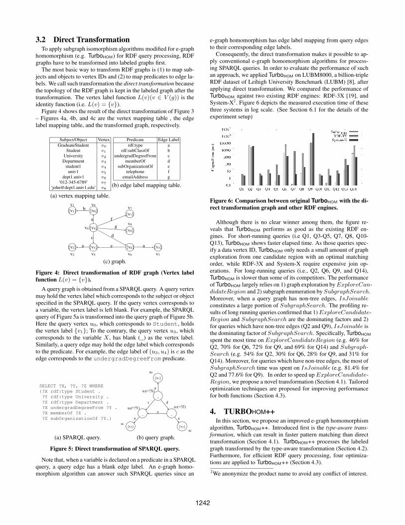
Consequently, the direct transformation makes it possible to ap-ply conventional e-graph homomorphism algorithms for process-ing SPARQL queries. In order to evaluate the performance of suchan approach, we applied TurboHOM on LUBM8000, a billion-tripleRDF dataset of Leihigh University Benchmark (LUBM) [8], afterapplying direct transformation. We compared the performance ofTurboHOM against two existing RDF engines: RDF-3X [19], andSystem-X2. Figure 6 depicts the measured execution time of thesethree systems in log scale. (See Section 6.1 for the details of theexperiment setup)
Figure 6: Comparison between original TurboHOM with the di-rect transformation graph and other RDF engines.
Although there is no clear winner among them, the figure re-veals that TurboHOM performs as good as the existing RDF en-gines. For short-running queries (i.e Q1, Q3-Q5, Q7, Q8, Q10-Q13), TurboHOM shows faster elapsed time. As those queries spec-ify a data vertex ID, TurboHOM only needs a small amount of graphexploration from one candidate region with an optimal matchingorder, while RDF-3X and System-X require expensive join op-erations. For long-running queries (i.e., Q2, Q6, Q9, and Q14),TurboHOM is slower than some of its competitors. The performanceof TurboHOM largely relies on 1) graph exploration byExploreCan-didateRegion and 2) subgraph enumeration by SubgraphSearch.Moreover, when a query graph has non-tree edges, IsJoinableconstitutes a large portion of SubgraphSearch. The profiling re-sults of long running queries confirmed that 1)ExploreCandidate-Region and SubgraphSearch are the dominating factors and 2)for queries which have non-tree edges (Q2 and Q9), IsJoinable isthe dominating factor of SubgraphSearch. Specifically, TurboHOM
spent the most time on ExploreCandidateRegion (e.g. 46% forQ2, 70% for Q6, 72% for Q9, and 69% for Q14) and Subgraph-Search (e.g. 54% for Q2, 30% for Q6, 28% for Q9, and 31% forQ14). Moreover, for queries which have non-tree edges, the most ofSubgraphSearch time was spent on IsJoinable (e.g. 81.4% forQ2 and 77.6% for Q9). In order to speed upExploreCandidate-Region, we propose a novel transformation (Section 4.1). Tailoredoptimization techniques are proposed for improving performancefor both functions (Section 4.3).
4. TURBOHOM++In this section, we propose an improved e-graph homomorphism
algorithm, TurboHOM++. Introduced first is the type-aware trans-formation, which can result in faster pattern matching than directtransformation (Section 4.1). TurboHOM++ processes the labeledgraph transformed by the type-aware transformation (Section 4.2).Furthermore, for efficient RDF query processing, four optimiza-tions are applied to TurboHOM++ (Section 4.3).2We anonymize the product name to avoid any conflict of interest.
1242
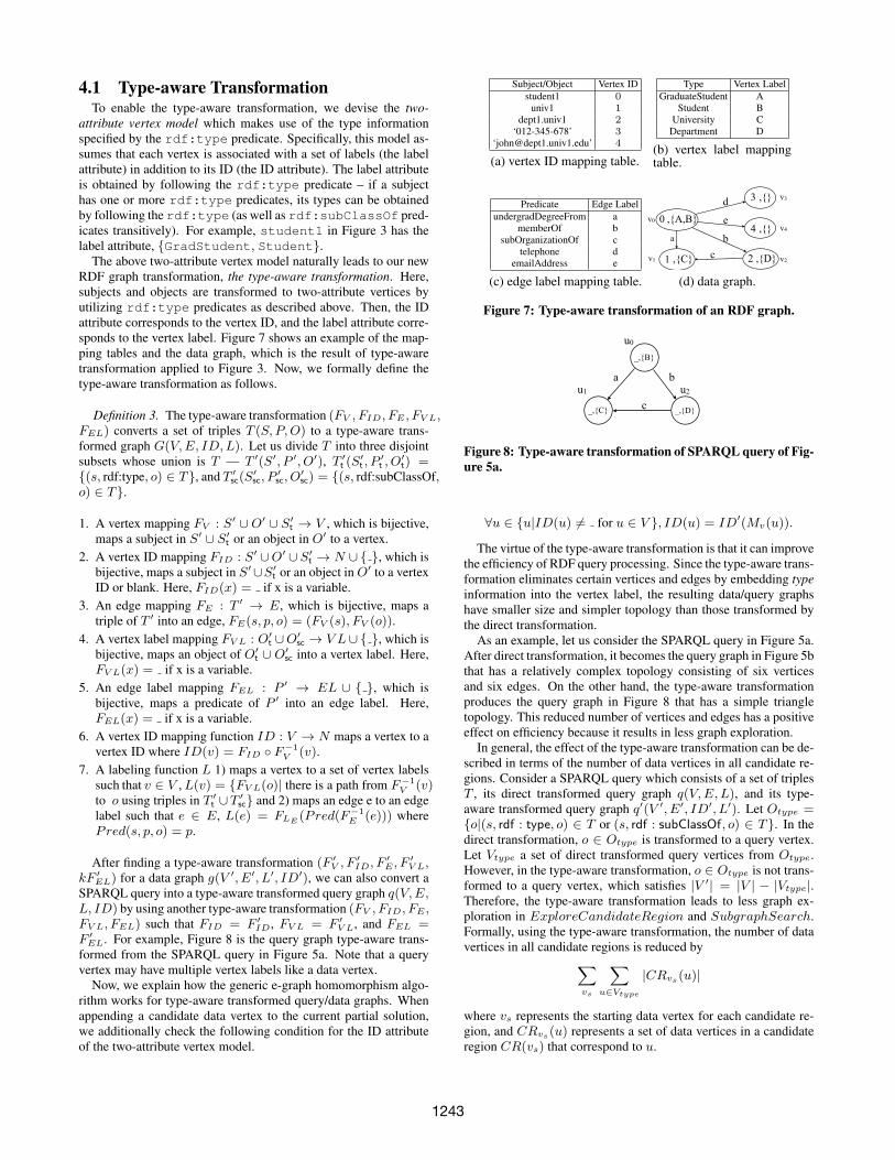
4.1 Type-aware TransformationTo enable the type-aware transformation, we devise the two-
attribute vertex model which makes use of the type informationspecified by the rdf:type predicate. Specifically, this model as-sumes that each vertex is associated with a set of labels (the labelattribute) in addition to its ID (the ID attribute). The label attributeis obtained by following the rdf:type predicate – if a subjecthas one or more rdf:type predicates, its types can be obtainedby following the rdf:type (as well as rdf:subClassOf pred-icates transitively). For example, student1 in Figure 3 has thelabel attribute, {GradStudent, Student}.
The above two-attribute vertex model naturally leads to our newRDF graph transformation, the type-aware transformation. Here,subjects and objects are transformed to two-attribute vertices byutilizing rdf:type predicates as described above. Then, the IDattribute corresponds to the vertex ID, and the label attribute corre-sponds to the vertex label. Figure 7 shows an example of the map-ping tables and the data graph, which is the result of type-awaretransformation applied to Figure 3. Now, we formally define thetype-aware transformation as follows.
Definition 3. The type-aware transformation (FV , FID, FE , FV L,FEL) converts a set of triples T (S, P,O) to a type-aware trans-formed graph G(V,E, ID,L). Let us divide T into three disjointsubsets whose union is T — T ′(S′, P ′, O′), T ′t (S′t , P ′t , O′t) ={(s, rdf:type, o) ∈ T}, and T ′sc(S′sc, P ′sc, O′sc) = {(s, rdf:subClassOf,o) ∈ T}.
1. A vertex mapping FV : S′ ∪ O′ ∪ S′t → V , which is bijective,maps a subject in S′ ∪ S′t or an object in O′ to a vertex.
2. A vertex ID mapping FID : S′ ∪O′ ∪ S′t → N ∪ { }, which isbijective, maps a subject in S′∪S′t or an object inO′ to a vertexID or blank. Here, FID(x) = if x is a variable.
3. An edge mapping FE : T ′ → E, which is bijective, maps atriple of T ′ into an edge, FE(s, p, o) = (FV (s), FV (o)).
4. A vertex label mapping FV L : O′t ∪O′sc → V L∪ { }, which isbijective, maps an object of O′t ∪ O′sc into a vertex label. Here,FV L(x) = if x is a variable.
5. An edge label mapping FEL : P ′ → EL ∪ { }, which isbijective, maps a predicate of P ′ into an edge label. Here,FEL(x) = if x is a variable.
6. A vertex ID mapping function ID : V → N maps a vertex to avertex ID where ID(v) = FID ◦ F−1
V (v).7. A labeling function L 1) maps a vertex to a set of vertex labels
such that v ∈ V ,L(v) = {FV L(o)| there is a path from F−1V (v)
to o using triples in T ′t ∪T ′sc} and 2) maps an edge e to an edgelabel such that e ∈ E, L(e) = FLE (Pred(F−1
E (e))) wherePred(s, p, o) = p.
After finding a type-aware transformation (F ′V , F′ID, F
′E , F
′V L,
kF ′EL) for a data graph g(V ′, E′, L′, ID′), we can also convert aSPARQL query into a type-aware transformed query graph q(V,E,L, ID) by using another type-aware transformation (FV , FID, FE ,FV L, FEL) such that FID = F ′ID , FV L = F ′V L, and FEL =F ′EL. For example, Figure 8 is the query graph type-aware trans-formed from the SPARQL query in Figure 5a. Note that a queryvertex may have multiple vertex labels like a data vertex.
Now, we explain how the generic e-graph homomorphism algo-rithm works for type-aware transformed query/data graphs. Whenappending a candidate data vertex to the current partial solution,we additionally check the following condition for the ID attributeof the two-attribute vertex model.
Subject/Object Vertex IDstudent1 0
univ1 1dept1.univ1 2
‘012-345-678’ 3‘[email protected]’ 4
(a) vertex ID mapping table.
Type Vertex LabelGraduateStudent A
Student BUniversity C
Department D
(b) vertex label mappingtable.
Predicate Edge LabelundergradDegreeFrom a
memberOf bsubOrganizationOf c
telephone demailAddress e
(c) edge label mapping table.
a bc
d
e0
3
4
21
,{A,B}
,{}
,{}
,{C} ,{D}
v0
v1
v3
v2
v4
(d) data graph.
Figure 7: Type-aware transformation of an RDF graph.
a b
c_,{C}
_,{B}
_,{D}
u0
u1 u2
Figure 8: Type-aware transformation of SPARQL query of Fig-ure 5a.
∀u ∈ {u|ID(u) 6= for u ∈ V }, ID(u) = ID′(Mv(u)).
The virtue of the type-aware transformation is that it can improvethe efficiency of RDF query processing. Since the type-aware trans-formation eliminates certain vertices and edges by embedding typeinformation into the vertex label, the resulting data/query graphshave smaller size and simpler topology than those transformed bythe direct transformation.
As an example, let us consider the SPARQL query in Figure 5a.After direct transformation, it becomes the query graph in Figure 5bthat has a relatively complex topology consisting of six verticesand six edges. On the other hand, the type-aware transformationproduces the query graph in Figure 8 that has a simple triangletopology. This reduced number of vertices and edges has a positiveeffect on efficiency because it results in less graph exploration.
In general, the effect of the type-aware transformation can be de-scribed in terms of the number of data vertices in all candidate re-gions. Consider a SPARQL query which consists of a set of triplesT , its direct transformed query graph q(V,E, L), and its type-aware transformed query graph q′(V ′, E′, ID′, L′). Let Otype ={o|(s, rdf : type, o) ∈ T or (s, rdf : subClassOf, o) ∈ T}. In thedirect transformation, o ∈ Otype is transformed to a query vertex.Let Vtype a set of direct transformed query vertices from Otype.However, in the type-aware transformation, o ∈ Otype is not trans-formed to a query vertex, which satisfies |V ′| = |V | − |Vtype|.Therefore, the type-aware transformation leads to less graph ex-ploration in ExploreCandidateRegion and SubgraphSearch.Formally, using the type-aware transformation, the number of datavertices in all candidate regions is reduced by∑
vs
∑u∈Vtype
|CRvs(u)|
where vs represents the starting data vertex for each candidate re-gion, and CRvs(u) represents a set of data vertices in a candidateregion CR(vs) that correspond to u.
1243
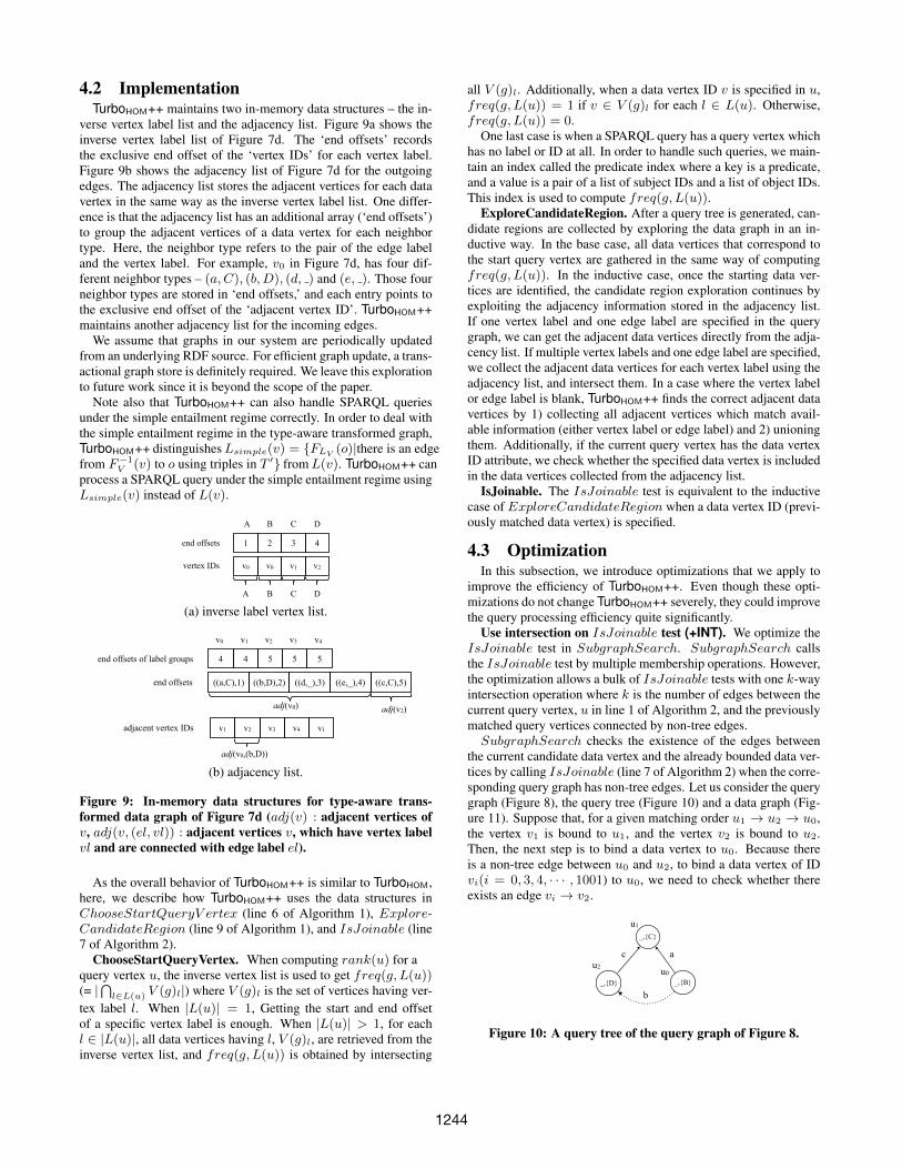
4.2 ImplementationTurboHOM++ maintains two in-memory data structures – the in-
verse vertex label list and the adjacency list. Figure 9a shows theinverse vertex label list of Figure 7d. The ‘end offsets’ recordsthe exclusive end offset of the ‘vertex IDs’ for each vertex label.Figure 9b shows the adjacency list of Figure 7d for the outgoingedges. The adjacency list stores the adjacent vertices for each datavertex in the same way as the inverse vertex label list. One differ-ence is that the adjacency list has an additional array (‘end offsets’)to group the adjacent vertices of a data vertex for each neighbortype. Here, the neighbor type refers to the pair of the edge labeland the vertex label. For example, v0 in Figure 7d, has four dif-ferent neighbor types – (a,C), (b,D), (d, ) and (e, ). Those fourneighbor types are stored in ‘end offsets,’ and each entry points tothe exclusive end offset of the ‘adjacent vertex ID’. TurboHOM++maintains another adjacency list for the incoming edges.
We assume that graphs in our system are periodically updatedfrom an underlying RDF source. For efficient graph update, a trans-actional graph store is definitely required. We leave this explorationto future work since it is beyond the scope of the paper.
Note also that TurboHOM++ can also handle SPARQL queriesunder the simple entailment regime correctly. In order to deal withthe simple entailment regime in the type-aware transformed graph,TurboHOM++ distinguishesLsimple(v) = {FLV (o)|there is an edgefrom F−1
V (v) to o using triples in T ′} fromL(v). TurboHOM++ canprocess a SPARQL query under the simple entailment regime usingLsimple(v) instead of L(v).
4 4 5 5 5end offsets of label groups
v1 v2 v3 v4 v1adjacent vertex IDs
end offsets ((a,C),1) ((b,D),2) ((d,_),3) ((e,_),4) ((c,D),5)
1 2 3 4end offsets
v0 v0 v1 v2vertex IDs
A B C D
v0 v1 v2 v3 v4
A B C D
adj(v2)
adj(v0,(b,D))
adj(v0)
(a) inverse label vertex list.
4 4 5 5 5end offsets of label groups
v1 v2 v3 v4 v1adjacent vertex IDs
end offsets ((a,C),1) ((b,D),2) ((d,_),3) ((e,_),4) ((c,C),5)
1 2 3 4end offsets
v0 v0 v1 v2vertex IDs
A B C D
v0 v1 v2 v3 v4
A B C D
adj(v2)
adj(v0,(b,D))
adj(v0)
(b) adjacency list.
Figure 9: In-memory data structures for type-aware trans-formed data graph of Figure 7d (adj(v) : adjacent vertices ofv, adj(v, (el, vl)) : adjacent vertices v, which have vertex labelvl and are connected with edge label el).
As the overall behavior of TurboHOM++ is similar to TurboHOM,here, we describe how TurboHOM++ uses the data structures inChooseStartQueryV ertex (line 6 of Algorithm 1), Explore-CandidateRegion (line 9 of Algorithm 1), and IsJoinable (line7 of Algorithm 2).
ChooseStartQueryVertex. When computing rank(u) for aquery vertex u, the inverse vertex list is used to get freq(g, L(u))(= |
⋂l∈L(u) V (g)l|) where V (g)l is the set of vertices having ver-
tex label l. When |L(u)| = 1, Getting the start and end offsetof a specific vertex label is enough. When |L(u)| > 1, for eachl ∈ |L(u)|, all data vertices having l, V (g)l, are retrieved from theinverse vertex list, and freq(g, L(u)) is obtained by intersecting
all V (g)l. Additionally, when a data vertex ID v is specified in u,freq(g, L(u)) = 1 if v ∈ V (g)l for each l ∈ L(u). Otherwise,freq(g, L(u)) = 0.
One last case is when a SPARQL query has a query vertex whichhas no label or ID at all. In order to handle such queries, we main-tain an index called the predicate index where a key is a predicate,and a value is a pair of a list of subject IDs and a list of object IDs.This index is used to compute freq(g, L(u)).
ExploreCandidateRegion. After a query tree is generated, can-didate regions are collected by exploring the data graph in an in-ductive way. In the base case, all data vertices that correspond tothe start query vertex are gathered in the same way of computingfreq(g, L(u)). In the inductive case, once the starting data ver-tices are identified, the candidate region exploration continues byexploiting the adjacency information stored in the adjacency list.If one vertex label and one edge label are specified in the querygraph, we can get the adjacent data vertices directly from the adja-cency list. If multiple vertex labels and one edge label are specified,we collect the adjacent data vertices for each vertex label using theadjacency list, and intersect them. In a case where the vertex labelor edge label is blank, TurboHOM++ finds the correct adjacent datavertices by 1) collecting all adjacent vertices which match avail-able information (either vertex label or edge label) and 2) unioningthem. Additionally, if the current query vertex has the data vertexID attribute, we check whether the specified data vertex is includedin the data vertices collected from the adjacency list.
IsJoinable. The IsJoinable test is equivalent to the inductivecase of ExploreCandidateRegion when a data vertex ID (previ-ously matched data vertex) is specified.
4.3 OptimizationIn this subsection, we introduce optimizations that we apply to
improve the efficiency of TurboHOM++. Even though these opti-mizations do not change TurboHOM++ severely, they could improvethe query processing efficiency quite significantly.
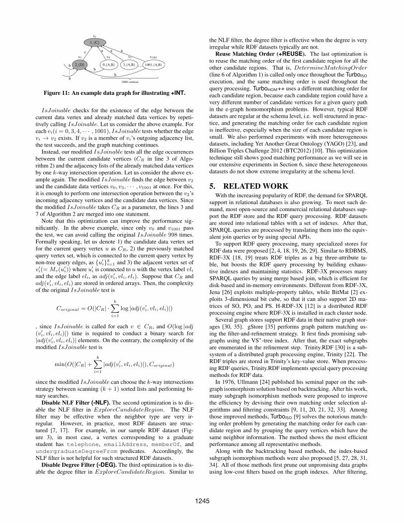
Use intersection on IsJoinable test (+INT). We optimize theIsJoinable test in SubgraphSearch. SubgraphSearch callsthe IsJoinable test by multiple membership operations. However,the optimization allows a bulk of IsJoinable tests with one k-wayintersection operation where k is the number of edges between thecurrent query vertex, u in line 1 of Algorithm 2, and the previouslymatched query vertices connected by non-tree edges.SubgraphSearch checks the existence of the edges between
the current candidate data vertex and the already bounded data ver-tices by calling IsJoinable (line 7 of Algorithm 2) when the corre-sponding query graph has non-tree edges. Let us consider the querygraph (Figure 8), the query tree (Figure 10) and a data graph (Fig-ure 11). Suppose that, for a given matching order u1 → u2 → u0,the vertex v1 is bound to u1, and the vertex v2 is bound to u2.Then, the next step is to bind a data vertex to u0. Because thereis a non-tree edge between u0 and u2, to bind a data vertex of IDvi(i = 0, 3, 4, · · · , 1001) to u0, we need to check whether thereexists an edge vi → v2.
{C}
{D}
b
{A,B}
a
{A,B}
a
{A,B}
a
…
c a
b_,{D}
_,{C}
_,{B}u0
u1
u2
} }1000 vertices
v1
v2 v0 v3 v1001
b a
_,{D}
_,{C}
_,{B}u0
u1
u2
Figure 10: A query tree of the query graph of Figure 8.
1244
bb
b
b…
2,{D}
c
0,{A,B}
a
3,{A,B}
a
1001,{A,B}
a
…
1, {C}
1000 vertices
v1
v2 v0 v3 v1001
Figure 11: An example data graph for illustrating +INT.
IsJoinable checks for the existence of the edge between thecurrent data vertex and already matched data vertices by repeti-tively calling IsJoinable. Let us consider the above example. Foreach vi(i = 0, 3, 4, · · · , 1001), IsJoinable tests whether the edgevi → v2 exists. If v2 is a member of vi’s outgoing adjacency list,the test succeeds, and the graph matching continues.
Instead, our modified IsJoinable tests all the edge occurrencesbetween the current candidate vertices (CR in line 3 of Algo-rithm 2) and the adjacency lists of the already matched data verticesby one k-way intersection operation. Let us consider the above ex-ample again. The modified IsJoinable finds the edge between v2and the candidate data vertices v0, v3, · · · , v1001 at once. For this,it is enough to perform one intersection operation between the v2’sincoming adjacency vertices and the candidate data vertices. Sincethe modified IsJoinable takes CR as a parameter, the lines 3 and7 of Algorithm 2 are merged into one statement.
Note that this optimization can improve the performance sig-nificantly. In the above example, since only v0 and v1001 passthe test, we can avoid calling the original IsJoinable 998 times.Formally speaking, let us denote 1) the candidate data vertex setfor the current query vertex u as CR, 2) the previously matchedquery vertex set, which is connected to the current query vertex bynon-tree query edges, as {u′i}ki=1 and 3) the adjacent vertex set ofv′i(=Mv(u
′i)) where u′i is connected to u with the vertex label vli
and the edge label eli, as adj(v′i, vli, eli). Suppose that CR andadj(v′i, vli, eli) are stored in ordered arrays. Then, the complexityof the original IsJoinable test is
Coriginal = O(|CR| ·k∑i=1
log |adj(v′i, vli, eli)|)
, since IsJoinable is called for each v ∈ CR, and O(log |adj(v′i, vli, eli)|) time is required to conduct a binary search for|adj(v′i, vli, eli)| elements. On the contrary, the complexity of themodified IsJoinable test is
min(O(|CR|+k∑i=1
|adj(v′i, vli, eli)|), Coriginal)
since the modified IsJoinable can choose the k-way intersectionsstrategy between scanning (k + 1) sorted lists and performing bi-nary searches.
Disable NLF Filter (-NLF). The second optimization is to dis-able the NLF filter in ExploreCandidateRegion. The NLFfilter may be effective when the neighbor type are very ir-regular. However, in practice, most RDF datasets are struc-tured [7, 17]. For example, in our sample RDF dataset (Fig-ure 3), in most case, a vertex corresponding to a graduatestudent has telephone, emailAddress, memberOf, andundergraduateDegreeFrom predicates. Accordingly, theNLF filter is not helpful for such structured RDF datasets.
Disable Degree Filter (-DEG). The third optimization is to dis-able the degree filter in ExploreCandidateRegion. Similar to
the NLF filter, the degree filter is effective when the degree is veryirregular while RDF datasets typically are not.
Reuse Matching Order (+REUSE). The last optimization isto reuse the matching order of the first candidate region for all theother candidate regions. That is, DetermineMatchingOrder(line 6 of Algorithm 1) is called only once throughout the TurboISO
execution, and the same matching order is used throughout thequery processing. TurboHOM++ uses a different matching order foreach candidate region, because each candidate region could have avery different number of candidate vertices for a given query pathin the e-graph homomorphism problems. However, typical RDFdatasets are regular at the schema level, i.e. well structured in prac-tice, and generating the matching order for each candidate regionis ineffective, especially when the size of each candidate region issmall. We also performed experiments with more heterogeneousdatasets, including Yet Another Great Ontology (YAGO) [23], andBillion Triples Challenge 2012 (BTC2012) [10]. This optimizationtechnique still shows good matching performance as we will see inour extensive experiments in Section 6, since these heterogeneousdatasets do not show extreme irregularity at the schema level.
5. RELATED WORKWith the increasing popularity of RDF, the demand for SPARQL
support in relational databases is also growing. To meet such de-mand, most open-source and commercial relational databases sup-port the RDF store and the RDF query processing. RDF datasetsare stored into relational tables with a set of indexes. After that,SPARQL queries are processed by translating them into the equiv-alent join queries or by using special APIs.
To support RDF query processing, many specialized stores forRDF data were proposed [2, 4, 18, 19, 26, 29]. Similar to RDBMS,RDF-3X [18, 19] treats RDF triples as a big three-attribute ta-ble, but boosts the RDF query processing by building exhaus-tive indexes and maintaining statistics. RDF-3X processes manySPARQL queries by using merge based join, which is efficient fordisk-based and in-memory environments. Different from RDF-3X,Jena [26] exploits multiple-property tables, while BitMat [2] ex-ploits 3-dimensional bit cube, so that it can also support 2D ma-trices of SO, PO, and PS. H-RDF-3X [12] is a distributed RDFprocessing engine where RDF-3X is installed in each cluster node.
Several graph stores support RDF data in their native graph stor-ages [30, 35]. gStore [35] performs graph pattern matching us-ing the filter-and-refinement strategy. It first finds promising sub-graphs using the VS∗-tree index. After that, the exact subgraphsare enumerated in the refinement step. Trinity.RDF [30] is a sub-system of a distributed graph processing engine, Trinity [22]. TheRDF triples are stored in Trinity’s key-value store. When process-ing RDF queries, Trinity.RDF implements special query processingmethods for RDF data.
In 1976, Ullmann [24] published his seminal paper on the sub-graph isomorphism solution based on backtracking. After his work,many subgraph isomorphism methods were proposed to improvethe efficiency by devising their own matching order selection al-gorithms and filtering constraints [9, 11, 20, 21, 32, 33]. Amongthose improved methods, TurboISO [9] solves the notorious match-ing order problem by generating the matching order for each can-didate region and by grouping the query vertices which have thesame neighbor information. The method shows the most efficientperformance among all representative methods.
Along with the backtracking based methods, the index-basedsubgraph isomorphism methods were also proposed [5, 27, 28, 31,34]. All of those methods first prune out unpromising data graphsusing low-cost filters based on the graph indexes. After filtering,
1245

any subgraph isomorphism methods can be applied to those un-filtered data graphs. This technique is only useful when there aremany small data graphs. Thus, these index-based subgraph isomor-phism methods do not enhance RDF graph processing since thereis only one big graph in an RDF database.
6. EXPERIMENTSWe perform extensive experiments on large-scale real and syn-
thetic datasets in order to show the superiority of a tamed subgraphisomorphism algorithm for RDF query processing. In the experi-ment, we use TurboHOM++. We assume that TurboHOM uses directtransformation, while TurboHOM++ uses type-aware transforma-tion along with all optimizations. The specific goals of the exper-iments are 1) We show the superior performance of TurboHOM++over the state-of-the-art RDF engines (Section 6.2), 2) We analyzethe effect of the type-aware transformation and the series of opti-mizations (Section 6.3), and 3) We show the linear speed-up of theparallel TurboHOM++ with an increasing number of threads (Dueto the space limit, please refer [13] for the detailed result).
6.1 Experiment SetupCompetitors. We choose three representative RDF engines as
competitors of TurboHOM++ – RDF-3X, TripleBit, and System-X.Note that these three systems are publicly available. RDF-3X [19]is a well-known RDF store, showing good performance for vari-ous types of SPARQL queries. TripleBit [29] is a very recent RDFengine efficiently handling large-scale RDF data. System-X is apopular RDF engine exploiting bitmap indexing. We exclude Bit-Mat [2] from performance evaluation since it is clearly inferior toTripleBit [29]. gStore is excluded since it is not publicly available.
Datasets. We use four RDF datasets in the experiment – LUBM[8], YAGO [23], BTC2012 [10], and BSBM [3]. LUBM isa de-facto standard RDF benchmark which provides a syntheticdata generator. Using the generator, we create three datasets –LUBM80, LUBM800, and LUBM8000 where the number repre-sents the scaling factor. YAGO is a real dataset which consists offacts from Wikipedia and the WordNet. BTC2012 is a real datasetcrawled from multiple RDF web resources. Lastly, BSBM is anRDF benchmark which provides a synthetic data generator andbenchmark queries. BSBM uses more general SPARQL query fea-tures such as FILTER, OPTIONAL, and UNION. Due to the spacelimit, please refer [13] for the experimental results for YAGO sincethe performance trends of YAGO are similar to those for BTC2012.
In order to support the original benchmark queries in LUBM, weload the original triples as well as inferred triples into databases. Inorder to obtain inferred triples, we use the state-of-the-art RDF in-ference engine. For example, LUBM8000 contains 1068394687original triples and 869030729 inferred triples. Note that this is thestandard way to perform the LUBM benchmark. However, regard-ing BTC2012, we use the original triples only for database loading.This is because the BTC2012 dataset contains many triples that vi-olate the RDF standard, and thus the RDF inference engine refusesto load and execute inference for the BTC2012 dataset. BSBMcontains 986410726 original triples and 11412064 inferred triples.
Table 1 shows the number of vertices and edges of the graphstransformed by the direct transformation and the type-ware trans-formation. The reduced number of edges in the type-aware trans-formed graph directly affects the amount of graph exploration ine-graph homomorphism matching.
Queries. Regarding LUBM, we use the 14 original benchmarkqueries provided in the website3. Previous work such as [29] and
3http://swat.cse.lehigh.edu/projects/lubm/
Table 1: Graph size statistics (direct: direct transformation,type-aware: type-aware transformation).
|V | direct |E| direct |V | type-aware |E| type-awareLUBM80 2644579 19461754 2644573 12357312LUBM800 26304872 193691328 26304863 122994224LUBM8000 263133301 1937425416 263133295 1230263406BTC2012 367728453 1436545556 367459811 1185887764BSBM 223938701 997822791 1937425416 893575906
[30] modified some of the original queries because executing thoseoriginal queries without the inferred triples returns an empty resultset. Regarding BTC2012, we use the same query sets proposedin [29], because they do not have official benchmark queries. Re-garding BSBM, we used 12 queries in the explore use case 4 whichcontain OPTIONAL, FILTER, and UNION keywords which testthe capability of more general SPARQL query support.
In order to measure the pure subgraph matching performance, (1)we omit modifiers which reorganize the subgraph pattern matchingresults (e.g. DISTINCT and ORDER BY) in all queries and (2) wemeasure the elapsed time excluding the dictionary look-up time.
Running Environment. We conduct the experiments in a serverrunning Linux four Intel Xeon E5-4640 CPUs and 1.5TB RAM.The server has the NUMA [15, 16] architecture with 4 sockets inwhich each socket has its own CPU and local memory.
We measure the elapsed times with a warm cache. To do that,we set up the competitors’ running environment as follows. ForRDF-3X and TripleBit, as done in [30], we put the database files inthe tmpfs in-memory filesystem, which is a kind of RAM disk. ForSystem-X, we set the memory buffer size to 400GB, which is suf-ficient for loading the entire database in memory. We execute everyquery five times, exclude the best and worst times, and compute theaverage of the remaining three.
6.2 Comparison between TurboHOM++ andRDF engines
We report the elapsed times of the benchmark queries using asingle thread. Since the server has a NUMA architecture, memoryallocation is always done within one CPU’s local memory.
LUBM. Table 2 shows the number of solutions for all bench-mark queries in all LUBM datasets. Table 3 shows experimen-tal results for LUBM80, LUBM800, and LUBM8000. Note thatTriplebit was not able to return correct answers for two queries overLUBM80/LUBM800 and for ten queries over LUBM8000. In Ta-ble 3, we use ’X’ or the superscript ‘*’ over the elapsed times whenTripleBit returns incorrect numbers of solutions.
In order to analyze results in depth, we classify the LUBMqueries into two types. The first type of queries has a constant num-ber of solutions regardless of the dataset size. Q1, Q3 ˜ Q5, Q7,Q8, and Q10 ˜ Q12 belong to this type. These queries are calledconstant solution queries. The other queries (Q2, Q6, Q9, Q13,and Q14) have increasing numbers of solutions proportional to thedataset size. These queries are called increasing solution queries.
Regarding the constant solution queries, only TurboHOM++achieves the ideal performance in LUBM, which means constantperformance regardless of dataset size. This phenomenon is an-alyzed as follows. Each constant solution query contains a queryvertex whose ID attribute is set to an entity in the RDF graph. Thus,TurboHOM++ chooses that query vertex as a starting query ver-tex and generates a candidate region. Furthermore, in the LUBM4http://wifo5-03.informatik.uni-mannheim.de/bizer/berlinsparqlbenchmark/spec/ExploreUseCase/index.html
1246
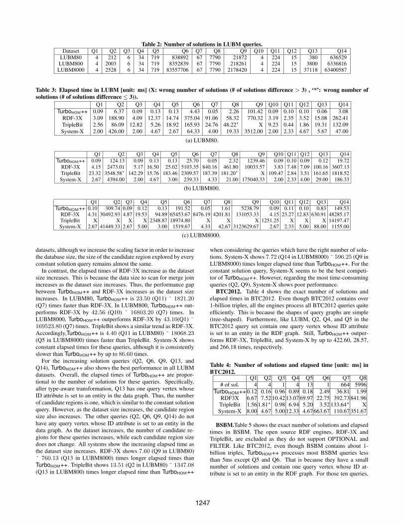
Table 2: Number of solutions in LUBM queries.Dataset Q1 Q2 Q3 Q4 Q5 Q6 Q7 Q8 Q9 Q10 Q11 Q12 Q13 Q14
LUBM80 4 212 6 34 719 838892 67 7790 21872 4 224 15 380 636529LUBM800 4 2003 6 34 719 8352839 67 7790 218261 4 224 15 3800 6336816
LUBM8000 4 2528 6 34 719 83557706 67 7790 2178420 4 224 15 37118 63400587
Table 3: Elapsed time in LUBM [unit: ms] (X: wrong number of solutions (# of solutions difference > 3) , ‘*’: wrong number ofsolutions (# of solutions difference ≤ 3)).
Q1 Q2 Q3 Q4 Q5 Q6 Q7 Q8 Q9 Q10 Q11 Q12 Q13 Q14TurboHOM++ 0.09 6.37 0.09 0.13 0.13 4.43 0.05 2.26 101.42 0.09 0.10 0.10 0.06 3.08
RDF-3X 3.09 188.90 4.09 12.37 14.74 375.04 91.06 58.32 770.32 3.19 2.35 3.52 15.08 262.41TripleBit 2.56 86.09 12.82 5.26 18.92 165.93 24.76 48.22∗ X 9.23 0.44 1.86 19.31 132.09System-X 2.00 426.00 2.00 4.67 2.67 64.33 4.00 19.33 3512.00 2.00 2.33 4.67 5.67 47.00
(a) LUBM80.
Q1 Q2 Q3 Q4 Q5 Q6 Q7 Q8 Q9 Q10 Q11 Q12 Q13 Q14TurboHOM++ 0.09 124.13 0.09 0.13 0.13 25.70 0.05 2.32 1239.46 0.09 0.10 0.09 0.12 19.72
RDF-3X 4.15 2473.01 5.17 16.50 25.02 5103.35 840.16 461.80 10033.57 3.83 7.48 7.09 100.16 3607.13TripleBit 23.32 3548.58∗ 142.29 15.76 183.46 2309.57 187.39 181.20∗ X 109.47 2.84 3.51 161.65 1818.52System-X 2.67 4394.00 2.00 4.67 3.00 239.33 4.33 21.00 175040.33 2.00 2.33 4.00 29.00 186.33
(b) LUBM800.
Q1 Q2 Q3 Q4 Q5 Q6 Q7 Q8 Q9 Q10 Q11 Q12 Q13 Q14TurboHOM++ 0.10 309.74 0.09 0.12 0.13 191.52 0.05 1.61 5238.79 0.09 0.11 0.10 0.83 149.53
RDF-3X 4.31 30492.93 4.87 19.53 94.89 65453.67 8476.19 4201.81 131053.33 4.15 23.27 12.83 630.91 48285.17TripleBit X X X X 2348.87 18974.80 X X X 1251.25 X X X 14197.47System-X 2.67 41449.33 2.67 5.00 3.00 1519.67 4.33 42.67 3123629.67 2.67 2.33 5.00 88.00 1155.00
(c) LUBM8000.
datasets, although we increase the scaling factor in order to increasethe database size, the size of the candidate region explored by everyconstant solution query remains almost the same.
In contrast, the elapsed times of RDF-3X increase as the datasetsize increases. This is because the data size to scan for merge joinincreases as the dataset size increases. Thus, the performance gapbetween TurboHOM++ and RDF-3X increases as the dataset sizeincreases. In LUBM80, TurboHOM++ is 23.50 (Q11) ˜ 1821.20(Q7) times faster than RDF-3X. In LUBM800, TurboHOM++ out-performs RDF-3X by 42.56 (Q10) ˜ 16803.20 (Q7) times. InLUBM8000, TurboHOM++ outperforms RDF-3X by 43.10(Q1) ˜169523.80 (Q7) times. TripleBit shows a similar trend as RDF-3X.Accordingly,TurboHOM++ is 4.40 (Q11 in LUBM80) ˜ 18068.23(Q5 in LUBM8000) times faster than TripleBit. System-X showsconstant elapsed times for these queries, although it is consistentlyslower than TurboHOM++ by up to 86.60 times.
For the increasing solution queries (Q2, Q6, Q9, Q13, andQ14), TurboHOM++ also shows the best performance in all LUBMdatasets. Overall, the elapsed times of TurboHOM++ are propor-tional to the number of solutions for these queries. Specifically,after type-aware transformation, Q13 has one query vertex whoseID attribute is set to an entity in the data graph. Thus, the numberof candidate regions is one, which is similar to the constant solutionquery. However, as the dataset size increases, the candidate regionsize also increases. The other queries (Q2, Q6, Q9, Q14) do nothave any query vertex whose ID attribute is set to an entity in thedata graph. As the dataset increases, the number of candidate re-gions for these queries increases, while each candidate region sizedoes not change. All systems show the increasing elapsed time asthe dataset size increases. RDF-3X shows 7.60 (Q9 in LUBM80)˜ 760.13 (Q13 in LUBM8000) times longer elapsed times thanTurboHOM++. TripleBit shows 13.51 (Q2 in LUBM80) ˜ 1347.08(Q13 in LUBM800) times longer elapsed time than TurboHOM++
when considering the queries which have the right number of solu-tions. System-X shows 7.72 (Q14 in LUBM8000) ˜ 596.25 (Q9 inLUBM8000) times longer elapsed time than TurboHOM++. For theconstant solution query, System-X seems to be the best competi-tor of TurboHOM++. However, regarding the most time-consumingqueries (Q2, Q9), System-X shows poor performance.
BTC2012. Table 4 shows the exact number of solutions andelapsed times in BTC2012. Even though BTC2012 contains over1-billion triples, all the engines process all BTC2012 queries quiteefficiently. This is because the shapes of query graphs are simple(tree-shaped). Furthermore, like LUBM, Q2, Q4, and Q5 in theBTC2012 query set contain one query vertex whose ID attributeis set to an entity in the RDF graph. Still, TurboHOM++ outper-forms RDF-3X, TripleBit, and System-X by up to 422.60, 28.57,and 266.18 times, respectively.
Table 4: Number of solutions and elapsed time [unit: ms] inBTC2012.
Q1 Q2 Q3 Q4 Q5 Q6 Q7 Q8# of sol. 4 4 1 4 13 1 664 5996
TurboHOM++ 0.12 0.16 0.96 0.89 0.18 2.49 36.81 1.99RDF3X 6.67 7.52 10.42 13.07 69.97 22.75 392.73 841.96TripleBit 1.56 1.81∗ 0.98 6.94 5.20 3.52 133.64∗ XSystem-X 8.00 4.67 5.00 12.33 4.67 663.67 110.67 351.67
BSBM.Table 5 shows the exact number of solutions and elapsedtimes in BSBM. The open source RDF engines, RDF-3X andTripleBit, are excluded as they do not support OPTIONAL andFILTER. Like BTC2012, even though BSBM contains about 1-billion triples, TurboHOM++ processes most BSBM queries lessthan 5ms except Q5 and Q6. That is because they have a smallnumber of solutions and contain one query vertex whose ID at-tribute is set to an entity in the RDF graph. For those ten queries,
1247

TurboHOM++ outperforms System-X by 2.37 ˜ 7284.47 times. Q5and Q6 take longer than the other queries because they use expen-sive filters such as join conditions (Q5) and a regular expression(Q6) and filter out a large number of solutions after basic graphpattern matching is finished. Before evaluating FILTER, Q5 (Q6)has 178030 (2848000) solutions from the query graph pattern andonly qualifies 6803 (43508) final solutions.
Table 5: Number of solutions and elapsed time [unit: ms] inBSBM.
Q1 Q2 Q3 Q4 Q5 Q6# of sol. 79 17 202 142 6803 43508
TurboHOM++ 0.58 0.15 8.15 1.27 344.66 3969.18System-X 10 1092.67 19.33 21.67 589.67 9889.00
Q7 Q8 Q9 Q10 Q11 Q12# of sol. 2 1 21 3 10 1
TurboHOM++ 0.25 0.16 0.11 0.23 0.14 0.12System-X 23.33 12.33 4.00 11.00 3.00 8.00
6.3 Effect of Improvement TechniquesWe measure the effect of the improvement techniques including
the type-aware transformation (Section 4.1) and the four optimiza-tions (Section 4.3). For this purpose, we use the largest LUBMdataset, LUBM8000. We first show the effect of the type-awaretransformation because it is beneficial to all LUBM queries. Wenext show the effect of the four optimizations (Section 6.3.2).
6.3.1 Effect of Type-aware TransformationTable 6 shows the elapsed times for the LUBM queries in
LUBM8000 using the direct transformation (TurboHOM) and thetype-aware transformation (TurboHOM++ without optimizations).Compared with the direct transformation, the type-aware transfor-mation improves the query performance by 1.01(Q1) to 27.22(Q6).
The obvious reason for performance improvement is the smallerquery sizes after the type-aware transformation. The reduced sizedquery graph leads to smaller size candidate regions and shorterelapsed times. First of all, Q6 and Q14 benefit the most from thetype-aware transformation. After the type-aware transformation,these queries become point-shaped. That is, solutions of these twoqueries are directly obtained by iterating the data vertices whichhave the vertex label of the query vertex, which corresponds tolines 2–4 in Algorithm 1. Q13 also benefits much from the type-aware transformation, since the type-aware transformation choosesa better starting query vertex than the direct transformation whichchooses a query vertex having type information. Q1, Q3, Q4, Q5,Q7, Q8, Q10, Q11, and Q12 do not benefit from the type-awaretransformation because they already have a small number of candi-date vertices under the direct transformation.
Q2 benefits less than the other long running queries fromthe type-aware transformation. The following is the pro-filing result of Q2 with the direct/type-aware transformation.Q2 with direct transformation takes 26774.73 millisecondsin ExploreCandidateRegion and 31191.29 milliseconds inSubgraphSearch. Note that, with direct transformation, the start-ing vertex is arbitrarily chosen from u0, u1, u2 in Figure 5bsince they all have same vertex label frequency (freq(g, L(ui)) =1, i = 0, 1, 2) and the same degree of 1. In our implementa-tion, the first query vertex u0 is chosen and thus the label of thenon-tree edge is subOrganizationOf. However, with type-awaretransformation, the starting vertex is u1 in Figure 8, and the la-bel of the non-tree edge is memberOf. Although the number of
candidate regions with u1 is the minimum among u0, u1, and u2,the cost of IsJoinable calls for memberOf increases 1.30 times.Thus, Q2 with type-aware transformation takes 9523.60 millisec-onds in ExploreCandiateRegion and 40469.47 milliseconds inSubgraphSearch. We achieve only 1.16 times performance im-provement. However, the cost of the IsJoinable call is signif-icantly reduced by using +INT. Thus, after applying type-awaretransformation and the tailored optimizations, the final elapsed timefor Q2 becomes 309.74ms, i.e., 187.15 times performance im-provement compared with direct transformation only.
6.3.2 Effect of Four OptimizationsIn this experiment, we measure the effect of four optimizations
of TurboHOM++. We use Q2 and Q9 in LUBM8000 since these twoqueries in LUBM8000 are the most time-consuming and exploit alloptimizations. All the other queries are omitted since their elapsedtimes are too short, so that it is hard to recognize the effect of op-timization. Note that the elapsed times of Q1, Q3 ˜ Q5, Q7, Q8,Q10 ˜ Q13 are too short (< 2ms), and Q6 and Q14 do not benefitfrom these optimizations since they are point-shaped.
Figure 12 shows the reduced times of Q2 and Q9 in LUBM8000after applying these optimizations separately. The optimizationtechniques in X-axis are ordered by the reduced in a decreasingmanner — +INT, -NLF, -DEG, and +REUSE. Interestingly, eventhough Q2 and Q9 have the same shape (i.e., trianglular), the mosteffective optimizations were different. +INT was the most effectivein Q2. -NLF was the most effective in Q9 since the size of eachcandidate region was very small. -DEG was more effective in Q9than in Q2 since Q9 has more data vertices applied to the degreefilter. +REUSE was effective in Q9 which has large number ofcandidate regions while Q2 did not benefit from +REUSE.
Figure 12: Reduced elapsed time of each optimization (Elapsedtime of no-optimization: 50016.13ms (Q2) and 17829.50ms(Q9)).
7. CONCLUSIONThe core function of processing RDF data is subgraph pattern
matching. There have been two completely different directions forsupporting efficient subgraph pattern matching. One direction is todevelop specialized RDF query processing engines exploiting theproperties of RDF data, while the other direction is to develop effi-cient subgraph isomorphism algorithms for general, labeled graphs.In this paper, we posed an important research question, “Can sub-graph isomorphism be tamed for efficient RDF processing?” Inorder to address this question, we provided the first direct andcomprehensive comparison of the state-of-the-art subgraph isomor-phism method with representative RDF processing engines.
We first showed that a subgraph isomorphism algorithm requiresminimal modification to handle a graph homomorphism with edgelabel mapping which is the RDF graph pattern matching seman-tics. We then provided a novel transformation method, called
1248

Table 6: Effect of type-aware transformation in LUBM8000 (Performance gain = Direct transformation ÷ Type-aware transforma-tion).
Q1 Q2 Q3 Q4 Q5 Q6 Q7 Q8 Q9 Q10 Q11 Q12 Q13 Q14Direct transformation (ms) 0.101 57966.93 0.11 0.16 0.43 5218.47 0.15 5.63 114116.33 0.10 0.21 0.30 21.48 3886.43
Type-aware transformation (ms) 0.100 50016.13 0.09 0.14 0.13 191.69 0.05 1.73 17829.50 0.09 0.11 0.10 1.33 149.60Performance gain 1.01 1.16 1.23 1.09 3.34 27.22 2.80 3.25 6.40 1.14 1.95 3.01 16.17 25.98
type-aware transformation along with a series of optimization tech-niques. We next performed extensive experiments using RDFbenchmarks in order to show the superiority of the optimized sub-graph isomorphism over representative RDF processing engines.Experimental results showed that the optimized subgraph isomor-phism method achieved consistent and significant speedup overthose RDF processing engines.
This study drew a promising conclusion that a subgraph isomor-phism algorithm tamed for RDF processing can serve as an in-memory accelerator on top of a commercial RDF engine for real-time RDF query processing as well. We believe that this approachopens a new direction for RDF processing, so that both traditionaldirections can merge or benefit from each other.
AcknowledgmentThis work was supported in part by a gift from Oracle Labs’ Exter-nal Research Office. This work was also supported by the NationalResearch Foundation of Korea(NRF) grant funded by the Koreagovernment(MSIP) (No. NRF-2014R1A2A2A01004454) and theMSIP(Ministry of Science, ICT and Future Planning), Korea, un-der the “ICT Consilience Creative Program” (IITP-2015-R0346-15-1007) supervised by the IITP(Institute for Information & com-munications Technology Promotion).
References[1] D. J. Abadi et al. Sw-store: A vertically partitioned dbms for
semantic web data management. The VLDB Journal, 385–406, 2009.
[2] M. Atre et al. Matrix ”bit” loaded: A scalable lightweight joinquery processor for rdf data. In WWW ’10, 41–50.
[3] C. Bizer and A. Schultz. The berlin sparql benchmark. Inter-national Journal on Semantic Web and Information Systems(IJSWIS), 1–24, 2009.
[4] J. Broekstra et al. Sesame: A generic architecture for storingand querying rdf and rdf schema. In ISWC ’02, 54–68.
[5] J. Cheng et al. Fg-index: Towards verification-free query pro-cessing on graph databases. In SIGMOD ’07, 857–872.
[6] W. Fan et al. Graph homomorphism revisited for graphmatching. VLDB ’10, 1161–1172.
[7] A. Gubichev and T. Neumann. Exploiting the query structurefor efficient join ordering in SPARQL queries. In EDBT ’14,439–450.
[8] Y. Guo et al. Lubm: A benchmark for owl knowledge basesystems. Web Semant., 158–182, 2005.
[9] W.-S. Han et al. TurboISO: towards ultrafast and robust sub-graph isomorphism search in large graph databases. In SIG-MOD ’13, 337–348.
[10] A. Harth. Billion Triples Challenge data set. Downloadedfrom http://km.aifb.kit.edu/projects/btc-2012/, 2012.
[11] H. He and A. K. Singh. Graphs-at-a-time: Query languageand access methods for graph databases. In SIGMOD ’08,405–418.
[12] J. Huang, D. J. Abadi, and K. Ren. Scalable sparql queryingof large rdf graphs. VLDB ’11, 1123–1134.
[13] J. Kim et al. Taming subgraph isomorphism for rdf queryprocessing. Tr, 2015. URL http://wshan.net/download/TR/TurboHOM.pdf.
[14] J. Lee et al. An in-depth comparison of subgraph isomor-phism algorithms in graph databases. VLDB ’12, 133–144.
[15] V. Leis et al. Morsel-driven parallelism: A numa-aware queryevaluation framework for the many-core age. In SIGMOD’14, 743–754.
[16] Y. Li, I. Pandis, R. Muller, V. Raman, and G. M. Lohman.Numa-aware algorithms: the case of data shuffling. In CIDR,2013.
[17] T. Neumann and G. Moerkotte. Characteristic sets: Accuratecardinality estimation for rdf queries with multiple joins. InICDE ’11, 984 – 994.
[18] T. Neumann and G. Weikum. x-rdf-3x: fast querying, highupdate rates, and consistency for rdf databases. VLDB ’10,256–263.
[19] T. Neumann and G. Weikum. The rdf-3x engine for scalablemanagement of rdf data. The VLDB Journal, 91–113, 2010.
[20] L. P. Cordella et al. A (sub)graph isomorphism algorithmfor matching large graphs. IEEE Trans. Pattern Anal. Mach.Intell., 1367 – 1372, 2004.
[21] H. Shang et al. Taming verification hardness: An efficientalgorithm for testing subgraph isomorphism. VLDB ’08, 364–375.
[22] B. Shao et al. Trinity: A distributed graph engine on a mem-ory cloud. In SIGMOD ’13, 505–516.
[23] F. M. Suchanek et al. Yago: A large ontology from wikipediaand wordnet. Web Semant., 203–217, 2008.
[24] J. R. Ullmann. An algorithm for subgraph isomorphism. J.ACM, 31–42, 1976.
[25] C. Weiss et al. Hexastore: sextuple indexing for semantic webdata management. VLDB ’08, 1008–1019.
[26] K. Wilkinson and K. Wilkinson. Jena property table imple-mentation. In SSWS ’06, 35–46.
[27] X. Yan et al. Graph indexing: A frequent structure-basedapproach. In SIGMOD ’04, 335–346.
[28] X. Yan et al. Graph indexing based on discriminative fre-quent structure analysis. ACM Trans. Database Syst., 960–993, 2005.
[29] P. Yuan et al. Triplebit: a fast and compact system for largescale rdf data. VLDB ’13, 517–528.
[30] K. Zeng et al. A distributed graph engine for web scale rdfdata. VLDB ’13, 265–276.
[31] S. Zhang et al. Treepi: A novel graph indexing method. InICDE ’07, 966 – 975, .
[32] S. Zhang et al. Gaddi: Distance index based subgraph match-ing in biological networks. In EDBT ’09, 192–203, .
[33] P. Zhao and J. Han. On graph query optimization in largenetworks. VLDB ’10, 340–351.
[34] L. Zou et al. A novel spectral coding in a large graph database.In EDBT ’08, 181–192, .
[35] L. Zou et al. gstore: answering sparql queries via subgraphmatching. VLDB ’11, 482–493, .
1249