taming energy consumption variations in systems benchmarking

HAL Id: hal-02403379https://hal.inria.fr/hal-02403379

Submitted on 24 Jan 2020

HAL is a multi-disciplinary open accessarchive for the deposit and dissemination of sci-entific research documents, whether they are pub-lished or not. The documents may come fromteaching and research institutions in France orabroad, or from public or private research centers.

L’archive ouverte pluridisciplinaire HAL, estdestinée au dépôt et à la diffusion de documentsscientifiques de niveau recherche, publiés ou non,émanant des établissements d’enseignement et derecherche français ou étrangers, des laboratoirespublics ou privés.

Taming Energy Consumption Variations in SystemsBenchmarking

Zakaria Ournani, Mohammed Chakib Belgaid, Romain Rouvoy, Pierre Rust,Joël Penhoat, Lionel Seinturier

To cite this version:Zakaria Ournani, Mohammed Chakib Belgaid, Romain Rouvoy, Pierre Rust, Joël Penhoat, etal.. Taming Energy Consumption Variations in Systems Benchmarking. ICPE’2020 - 11thACM/SPEC International Conference on Performance Engineering, Apr 2020, Edmonton, Canada.�10.1145/3358960.3379142�. �hal-02403379�

https://hal.inria.fr/hal-02403379

https://hal.archives-ouvertes.fr

Taming Energy Consumption Variationsin Systems Benchmarking

Zakaria Ournani

Orange Labs/ Inria / Univ. Lille

[email protected]

Mohammed Chakib Belgaid

Inria / Univ. Lille

[email protected]

Romain Rouvoy

Univ. Lille / Inria / IUF

[email protected]

Pierre Rust

Orange Labs

[email protected]

Joel Penhoat

Orange Labs

[email protected]

Lionel Seinturier

Univ. Lille / Inria

[email protected]

ABSTRACT

The past decade witnessed the inclusion of power measurements

to evaluate the energy efficiency of software systems, thus making

energy a prime indicator along with performance. Nevertheless,

measuring the energy consumption of a software system remains

a tedious task for practitioners. In particular, the energy measure-

ment process may be subject to a lot of variations that hinder

the relevance of potential comparisons. While the state of the art

mostly acknowledged the impact of hardware factors (chip printing

process, CPU temperature), this paper investigates the impact of

controllable factors on these variations. More specifically, we con-

duct an empirical study of multiple controllable parameters that

one can easily tune to tame the energy consumption variations

when benchmarking software systems.

To better understand the causes of such variations, we ran more

than a 1, 000 experiments on more than 100 nodes with different

workloads and configurations. The main factors we studied encom-

pass: experimental protocol, CPU features (C-states, Turbo Boost,

core pinning) and generations, as well as the operating system.

Our experiments showed that, for some workloads, it is possible to

tighten the energy variation by up to 30×. Finally, we summarize

our results as guidelines to tame energy consumption variations.We

argue that the guidelines we deliver are the minimal requirements

to be considered prior to any energy efficiency evaluation.

CCS CONCEPTS

•Hardware→ Power and energy; Power estimation and optimiza-

tion; Platform power issue; Enterprise level and data centers power

issues.

KEYWORDS

Energy Variations; System Benchmarking; Energy Consumption;

Energy Efficiency

1 INTRODUCTION

To conduct robust evaluations, practitioners often try to ensure

reproducible environmental conditions in order to properly bench-

mark their software systems. In this area, reproducibility might

be achieved by ensuring the same execution settings of physical

nodes, virtual machines, clusters or cloud environments. Recently,

the research community has been investigating typical "crimes" in

systems benchmarking and established guidelines for conducting

robust and reproducible evaluations [23].

Node1 Node2 Node3 Node4Nodes

2400

2600

2800

3000

3200

3400

3600

Ener

gy C

onsu

mpt

ion

(mJ)

Figure 1: CPU energy variation for the benchmark CG

In theory, using identical CPU, samememory configuration, simi-

lar storage and networking capabilities, should favour reproducible

experiments. However, when it comes to measuring the energy

consumption of a system, applying acknowledged guidelines and

carefully repeating the same benchmark can nonetheless lead to dif-

ferent energy footprints not only on homogeneous nodes, but even

within a single node. This difference—also called energy variation(EV)—has become a serious threat to the accuracy of experimental

evaluations.

Figure 1 illustrates this variation problem as a violin plot of

20 executions of the benchmark Conjugate Gradient (CG) takenfrom the NAS Parallel Benchmarks (NBP) suite [3], on 4 nodes of

an homogeneous cluster (the cluster Dahu described in Table 1)

at 50 % workload. One can observe a large variation of the energy

consumption, not only among homogeneous nodes, but also at the

scale of a single node, reaching up to 25 % in this example.

Most of the state of the art has been investigating this power con-

sumption issue from a hardware perspective [5, 22] and reported

that the causes of such energy variations are CMOS manufacturing

process of transistors in a chip, differences in node assembly and

data center hot spots. Additionally, [13] described it as a combi-

nation of parameters, mentioning a list of candidate factors, such

as the thermal effect or the CPU frequency, but failing to deliver

a deeper analysis of these factors. Unfortunately, hardware fac-

tors can be hardly tuned to tame the energy variation that can be

observed in systems benchmarking. For example, managing the

CPU temperature or a server position in a cluster, are not actions

Conference’17, July 2017, Washington, DC, USA Zakaria Ournani, Mohammed Chakib Belgaid, Romain Rouvoy, Pierre Rust, Joel Penhoat, and Lionel Seinturier

that one can easily do, especially on the modern data centers and

cloud platforms. Therefore, the goal of this paper is to investigate

the spectrum of factors that can cause or increase the variability

of energy consumption in systems benchmarking, and to propose

effective guidelines to control such factors in order to mitigate this

variability. While this paper does not question the benefits of es-

tablished CPU features, like C-states or Turbo Boost, it delivers

a deeper analysis of the effects they may introduce on a wide set

of experiments and nodes. By quantifying potential energy vari-

ations induced by controllable factors, we intend to identify the

proper configurations that minimize energy variations, depending

on the workload characteristics. These guidelines aim at supporting

practitioners in conducting robust system benchmarks and report-

ing reproducible energy consumption, rather than recommending

production-scale practices or solutions to reduce the power con-

sumption of a given system. The key contributions of this paper

can therefore be summarized as:

(1) Providing a better understanding of the energy variation,

by using different generations of CPU deployed in 4 clus-

ters with more than 100 physical nodes, and by considering

existing systems benchmarks with diverse workloads;

(2) Identifying controllable factors that contribute to the varia-

tion in CPU energy consumption, comparing them against

the state of the art, and completing them with other uncov-

ered assumptions;

(3) Reporting on some guidelines on how to conduct repro-

ducible experiments with less energy variations;

(4) Discussing the differences between inter-nodes and intra-

nodes variations.

The remainder of this paper is organized as follows. Section 2

discusses the related works in the area of power measurements.

Section 3 formalizes our research questions. Section 4 reports on the

experimental setup (hardware, benchmarks, tools andmethodology)

we used in this work. Section 5 analyzes the causes of the variations

we observed along experiments. Finally, we discuss the results of

the different experimented factors, and their impact on the energy

variation in Section 6, while Sections 7 & 8 cover the validity threats

and our conclusions, respectively.

2 RELATEDWORK

In this section, we review the state of the art in the domain of

energy consumption analysis. In particular, one can observe that

several studies considered the evaluation of the processor variation

while executing the same workload, in particular to test distributed

applications running in homogeneous clusters.

Studying Hardware Factors. This variation has often been related

to the manufacturing process [7], but has also been a subject of

many studies, considering several aspects that could impact and

vary the energy consumption across executions and on different

chips. On the one hand, the correlation between the processor tem-

perature and the energy consumption was one of the most explored

paths. Kistowski et al. showed in [15] that identical processors can

exhibit significant energy consumption variation with no close

correlation with the processor temperature and performance. On

the other hand, the authors of [26] claimed that the processor ther-

mal effect is one of the most contributing factors to the energy

variation, and the correlation between the CPU temperature and

the energy consumption variation is very tight. This makes the

processor temperature a delicate factor to consider while compar-

ing energy consumption variations across a set of homogeneous

processors.

The ambient temperature was also discussed in many papers as

a candidate factor for the energy variation of a processor. In [24],

the authors claimed that energy consumption may vary due to

fluctuations caused by the external environment. These fluctuations

may alter the processor temperature and its energy consumption.

However, the temperature inside a data center does not show major

variations from one node to another. In [11], El Mehdi Dirouri et al.showed that switching the spot of two servers does not affect their

energy consumption. Moreover, changing hardware components,

such as the hard drive, the memory or even the power supply, does

not affect the energy variation of a node, making it mainly related

to the processor. This result was recently assessed by [26], where

the rack placement and power supply introduced a maximum of

2.8 % variation in the observed energy consumption.

Beyond hardware components, the accuracy of power meters

has also been questioned. Inadomi et al. [14] used three different

power measurement tools: RAPL, Power Insight1and BGQ EMON.

All of the three tools recorded the same 10% of energy variation,

that was supposedly related to the manufacturing process.

Mitigating Energy Variations. Acknowledging the energy varia-

tion problem on processors, some papers proposed contributions to

reduce and mitigate this variation. In [14], the authors introduced a

variation-aware algorithm that improves application performance

under a power constraint by determining module-level (individ-

ual processor and associated DRAM) power allocation, with up to

5.4× speedup. The authors of [12] proposed parallel algorithms

that tolerate the variability and the non-uniformity by decoupling

per process communication over the available CPU. Acun et al. [2]found out a way to reduce the energy variation on Ivy Bridge and

Sandy Bridge processors, by disabling the Turbo Boost feature to

stabilize the execution time over a set of processors. They also pro-

posed some guidelines to reduce this variation by replacing the old

slow chips, by load balancing the workload on the CPU cores and

leaving one core idle. They claimed that the variation between the

processor cores is insignificant. In [6], the researchers showed how

a parallel system can be used to deal with the energy variation by

compensating the uneven effects of power capping.

In [19], the authors highlight the increase of energy variation

across the latest Intel micro-architectures by a factor of 4 from

Sandy Bridge to Broadwell, a 15% of run-to-run variation within

the same processor and the increase of the inter-cores variation

from 2.5 % to 5 % due to hardware-enforced constraints, concluding

with some recommendations for Broadwell usage, such as running

one hyper-thread per core.

Objective. The aim of our paper is not to reproduce all the ex-

posed results and explored paths. Instead, we intend to check some

of these results on latest hardware components, and to consider

new potential controllable factors that could also contribute to the

1https://www.itssolution.com/products/trellis-power-insight-application

https://www.itssolution.com/products/trellis-power-insight-application

Taming Energy Consumption Variations in Systems Benchmarking Conference’17, July 2017, Washington, DC, USA

energy variation. We also aim to provide practitioners with guide-

lines to conduct robust experiments in a controlled environment,

thus reducing the variation overhead to share trustable results and

build credible comparisons.

3 RESEARCH QUESTIONS

Worth saying, we are aware that part of the energy consumption

variation is due to chip manufacturing differences or some of the

previously discussed enforced factors, such as the thermal effect

or the servers placement. Those parameters are often tricky to

manage, as we cannot have a perfect chips manufacturing process,

or assume that two identical processors have the same thermal

behavior. We will therefore focus on providing the practitioners

with an empirical study of some controllable parameters that can be

tuned to conduct experimental evaluations of energy consumption

with less variation, especially if the practitioners do not have a

physical access to the data center or BIOS configuration, which is

the case on most of the modern cloud platforms and data centers.

These parameters span the choice of the benchmarking protocol,

processor frequencies management, operating system tuning or

some other parameters. The authors of [13] mentioned some of

these potential parameters.

In this paper, we will therefore investigate the following control-

lable factors, which we formalize as 4 research questions:

RQ 1: Does the benchmarking protocol affect the energy vari-

ation?

RQ 2: How important is the impact of the processor features

on the energy variation?

RQ 3: What is the impact of the operating system on the energy

variation? and finally

RQ 4: Does the choice of the processor matter to mitigate the

energy variation?

4 EXPERIMENTAL SETUP

This section describes our detailed experimental environment, cov-

ering the clusters and nodes configuration, the benchmarks we

used and justifying our experimental methodology.

4.1 Hardware Platform

We considered 4 distinct clusters of variable sizes and different

generations of CPU, as summarized in Table 1. In particular, we

used the Grid5000 (G5K) platform in our experiments [4, 20]. G5K

is a bare metal cloud platform that can be used to provision clusters

of identical nodes. In our study, we mainly used the cluster Dahulocated in Grenoble to run most of our tests, as it has one of the

newest Xeon CPUs. We also used the clusters Chetemi, Ecotypeand Paranoia in some of our experiments. Table 1 describes the

configurations of the clusters we considered.

As most of the nodes are equipped with two sockets (physical

processors), we use the acronym CPU or socket to designate one

of the two sockets and PU for the operating system processingunit. The number of PU often doubles the number of available

cores because of the hyper-threading support, as the OS considers

2 hyper-threads sharing the same core as 2 different PU. Figure 2illustrates a detailed topology of a node belonging to the cluster

Dahu.

Table 1: Description of clusters included in the study

Cluster Processor Nodes RAM

Dahu 2× Intel XeonGold 6130 32 192GiB

Chetemi 2× Intel Xeon E5-2630v4 15 768GiB

Ecotype 2× Intel Xeon E5-2630Lv4 48 128GiB

Paranoia 2× Intel Xeon E5-2660v2 8 128GiB

Machine (192 GiB total)

Socket P#0

NUMANode P#0 (96GiB)

L3 (22MB)

L2 (1024KB)

L1d (32KB)

L1i (32KB)

PU P # 0

PU P # 32

Core P#0

L2 (1024KB)

L1d (32KB)

L1i (32KB)

PU P # 30

PU P # 62

Core P#15…

Socket P#1

NUMANode P#1 (96GiB)

L3 (22MB)

L2 (1024KB)

L1d (32KB)

L1i (32KB)

PU P # 1

PU P # 33

Core P#0

L2 (1024KB)

L1d (32KB)

L1i (32KB)

PU P # 31

PU P # 63

Core P#15…

Figure 2: Topology of the nodes of the cluster Dahu

4.2 Systems Benchmarks

Our first criterion to choose the systems benchmarks was the scal-

ability, as we need to run tests at different workloads by choosing

the right number of used PU. The other criteria are the documen-

tation, the accuracy and the references to the benchmark. NASParallel Benchmark (NPB v3.3.1) [3] is one of the most used suite of

benchmarks in the HPC literature and it fulfills our benchmarking

requirements. We mainly used the pseudo application Lower-Uppersymmetric Gauss-Seidel (LU), the Conjugate Gradient (CG) and Em-barrassingly Parallel (EP) computation-intensive benchmarks in our

experiments, with the C data class. These are the main benchmarks

used in many similar works, such as [13]. Nonetheless, in order to

validate our results on a wider set of benchmarks and applications,

we also used Stress-ng v0.10.0,2 pbzip2 v1.1.9,3 linpack4

and sha256 v8.265 as representative systems benchmarks to con-

duct our experiments with a broad diversity of workloads.

4.3 Measurement Tools & Methodology

To study the energy consumption of nodes, we considered Intel

Running Average Power Limit (RAPL) [16], which is one of the most

accurate tools to report the CPU/DRAM global energy consumption.

We also used PowerAPI [8], which is a power monitoring toolkit

that builds a model over RAPL to compute the energy consumption

at process-level when we needed to isolate energy consumption

of a single process. Our clusters are provisioned with a minimal

version of Debian 9 (4.9.0 kernel version) where we install Docker

(version 18.09.5), which will be used to run the RAPL sensor and

2https://kernel.ubuntu.com/~cking/stress-ng

3https://launchpad.net/pbzip2/

4http://www.netlib.org/linpack

5https://linux.die.net/man/1/sha256sum

https://kernel.ubuntu.com/~cking/stress-ng

https://launchpad.net/pbzip2/

http://www.netlib.org/linpack

https://linux.die.net/man/1/sha256sum


100 150 200 250 300STD (mJ)

0.000

0.002

0.004

0.006

0.008

0.010

0.012

0.014

0.016

Rate

DockerBinary

Figure 3: Comparing the variation of binary and Docker ver-

sions of aggregated LU, CG and EP benchmarks

the benchmark itself. The energy sensor collects RAPL reports and

stores them in a remoteMongoDB instance, allowing us to perform

post-mortem analysis in a dedicated environment. Using Docker

makes the deployment process easier on the one hand, and provides

us with a built-in control group encapsulation of the conducted

tests on the other hand. This allows PowerAPI to measures all the

running containers, even the RAPL sensor consumption, as it is

isolated in a container. One potential threat covers the impact of

Docker on the energy variation. We therefore conducted a prelimi-

nary experiment by running the same benchmarks LU, CG and EPin a Docker container and a flat binary format on 3 nodes of the

cluster Dahu to assess if Docker induces an additional variation.

Figure 3 reports that this is not the case, as the energy consumption

variation does not get noticeably affected by Docker while running

a same compiled version of the benchmarks at 5 %, 50 % and 100 %

workloads. In fact, while Docker increases the energy consumption

due to the extra layer it implements [9], it does not noticeably affect

the energy variation. The standard deviation (STD) is even slightly

smaller (STDDocker = 192mJ ,STDBinary = 207mJ ), taking into

account the measurements errors and the OS activity.

Every experiment is conducted on 100 iterations, on multiple

nodes and using the 3 NPB benchmarks we mentioned, with a

warmup phase of 10 iterations for each experiment. In most cases,

we were seeking to evaluate the STandard Deviation (STD), which

is the most representative factor of the energy variation. We tried

to be very careful, while running our experiments, not to fall in

the most common benchmarking "crimes" [23]. As we study the

STD difference of measurements we observed from empirical ex-

periments, we use the bootstrap method [10] to randomly build

multiple subsets of data from the original dataset, and we draw

the STD density of those sets, as illustrated in Figure 3. Given the

space constraints, this paper reports on aggregated results for nodes,

benchmarks and workloads, but the raw data we collected remains

available through the public repository we published.6We believe

this can help to achieve better and more reliable comparisons.

We mainly consider 3 different workloads in our experiments:

single process, 50 %, and 100 %, to cover the low, medium and high

6https://github.com/anonymous-data/Energy-Variation

CPU usage when analyzing the studied parameters effect, respec-

tively. These workloads reflect the ratio of used PU count to the

total available PU.

5 ENERGY VARIATION ANALYSIS

In this section, we aim to establish experimental guidelines to re-

duce the CPU energy variation. We therefore explore many poten-

tial factors and parameters that could have a considerable effect on

the energy variation.

5.1 RQ 1: Benchmarking Protocol

To achieve a robust and reproducible experiment, practitioners

often tend to repeat their tests multiple times, in order to analyze

the related performance indicators, such as execution time, memory

consumption or energy consumption. We therefore aim to study

the benchmarking protocol to identify how to efficiently iterate the

tests to capture a trustable energy consumption evaluation.

In this first experiment, we investigate if changing the testing

protocol affects the energy variation. To achieve this, we consid-

ered 3 execution modes: In the "normal" mode, we iteratively run

the benchmark 100 times without any extra command, while the

"sleep" mode suspends the execution script for 60 seconds between

iterations. Finally, the "reboot" mode automatically reboots the

machine after each iteration. The difference between the normaland sleep modes intends to highlight that the CPU needs some rest

before starting another iteration, especially for an intense workload.

Putting the CPU into sleep for several seconds could give it some

time to reach a lower frequency state or/and reduce its temperature,

which could have an impact on the energy variation. The rebootmode, on the other hand, is the most straightforward way to reset

the machine state after every iteration. It could also be beneficial to

reset the CPU frequency and temperature, the stored data, the cache

or the CPU registries. However, the reboot task takes a considerable

amount of time, so rebooting the node after every single operation

is not the fastest nor the most eco-friendly solution, but it deserves

to be checked to investigate if it effectively enhances the overall

energy variation or not.

Figure 4 reports on 300 aggregated executions of the benchmarks

LU, CG and EP, on 4 machines of the cluster Dahu (cf. Table 1) for

different workloads. We note that the results have been executed

with different datasets sizes (B, C and D for single process, 50 % and

100% respectively) to remedy to the brief execution times at high

workloads for small datasets. This justifies the scale differences of

reported energy consumptions between the 3 modes in Figure 4.

As one can observe, picking one of these strategies does not have a

strong impact on the energy variation for most workloads. In fact,

all the strategies seem to exhibit the same variation with all the

workloads we considered—i.e., the STD is tightly close between the

three modes. The only exception is the reboot mode at 100 % load,

where the STD is 150% times worst, due to an important amount

of outliers. This goes against our expectation, even when setting a

warm-up time after reboot to stabilize the OS.

In Figure 5, we study the standard deviation of the three modes

by constituting 5, 000 random 30-iterations sets from the previous

executions set and we compute the STD in each case, considering

mainly the 100% workload as the STD was 150% higher for the

https://github.com/anonymous-data/Energy-Variation


normal sleep reboot

Modes

7250

7500

7750

8000

8250

8500

8750

9000

Ener

gy C

onsu

mpt

ion

(mJ)

STD=290.85 mJ STD=242.23 mJSTD=260.6 mJSingle Process

normal sleep reboot

Modes

1700

1800

1900

2000

2100

STD=70.38 mJ STD=80.39 mJSTD=77.48 mJ

50%

normal sleep reboot

Modes

5750

6000

6250

6500

6750

7000

7250

STD=123.78 mJ STD=321.57 mJSTD=125.48 mJ100%

Figure 4: Energy variation with the normal, sleep and rebootmodes

100 200 300 400 500STD (mJ)

0.00

0.01

0.02

0.03

0.04

0.05

Rat

e

normalrebootsleep

Figure 5: STD analysis of the normal, sleep and rebootmodes

reboot mode with that load. We can observe that the considerable

amount of outliers in the reboot mode is not negligible, as the STD

density is clearly higher than the two other modes. This makes the

rebootmode as the less appropriate for the energy variation at high

workloads.

To answer RQ 1, we conclude that the benchmarking protocol

partially affects the energy variation, as highlighted by the

reboot mode results for high workloads.

5.2 RQ 2: Processor Features

The C-states provide the ability to switch the CPU between more

or less consuming states upon activities. Turning the C-states on

or off have been subject of many discussions [25], because of its

dynamic frequency mechanism but, to the best of our knowledge,

there have been no fully conducted C-states behavior analysis on

CPU energy variation.

We intend to investigate how much the energy consumption

varies when disabling the C-states (thus, keeping the CPU in the

C0 state) and at which workload. Figure 6 depicts the results of the

experiments we executed on three nodes of the cluster Dahu. Oneach node, we ran the same set of benchmarks with two modes:

C-states on, which is the default mode, and C-states off. Eachiteration includes 100 executions of the same benchmark at a given

workload, with three workload levels. We note that our results have

been confirmed with the benchmarks LU, CG and EP.We can clearly see the effect that has the C-states off mode

when running a single-process application/benchmark. The en-

ergy consumption varies 5 times less than the default mode. In

this case, only one CPU core is used among 2 × 16 physical cores.

The other cores are switched to a low consumption state when

C-states are on, the switching operation causes an important en-

ergy consumption difference between the cores, and could be af-

fected by other activities, such as the kernel activity, causing a

notable energy consumption variation. On the other hand, switch-

ing off the C-states would keep all the cores—even the unused

ones—at a high frequency usage. This highly reduces the varia-

tion, but causes up to 50 % of extra energy consumption in this test

(MeanC−states−of f = 11, 665mJ ,MeanC−states−on = 7, 641mJ ).At a 100% workload, disabling the C-states seems to have no

effect on the total energy consumption nor its variation. In fact, all

the cores are used at 100 % and the C-states module would have no

effect, as the cores are not idle. The same reason would apply for the

50 % load, as the hyper-threading is active on all cores, thus causing

the usage of most of them. For single process workloads, disabling

the C-states causes the process to consume 50% more energy as

reported in Figure 6, but reduces the variation by 5 times compared

to the C-states on mode. This leads to mainly two questions: Can a

process pinning method reduce/increase the energy variation? And,

how does the energy consumption variation evolve at different PU

usage level?

5.2.1 Cores Pinning. To answer the first question, we repeated

the previous test at 50 % workload. In this experiment, we consid-

ered three cores usage strategies, the first one (S1) would pin the

processes on all the PU of one of the two sockets (including hyper-

threads), so it will be used at 100 %, and leave the other CPU idle.

The second strategy (S2) splits the workload on the two sockets

so each CPU will handle 50 % of the load. In this strategy, we only

use the core PU and not the hyper-threads PU, so every process


C-states Off C-states OnModes

7000

8000

9000

10000

11000

12000

Ener

gy C

onsu

mpt

ion

(mJ)

STD = 53.17 mJ STD = 284.70 mJsingel Process


1700

1800

1900

2000

2100

Ener

gy C

onsu

mpt

ion

(mJ)

STD = 64.07 mJ STD = 68.21 mJ50%


6000

6500

7000

Ener

gy C

onsu

mpt

ion

(mJ)

STD=134.06 mJ STD=122.91 mJ100%

Figure 6: Energy variation when disabling the C-states

S1 S2 S3Modes

5000

10000

15000

20000

25000

30000

Ener

gy C

onsu

mpt

ion

(mJ)

Figure 7: Energy variation considering the three cores pin-

ning strategies at 50% workload

would not share his core usage (all the cores are being used). The

third strategy (S3) consists also on splitting the workload between

the two sockets, but considering the usage of the hyper-threads on

each core—i.e., half of the cores are being used over the two CPU.

Figure 7 reports on the energy consumption of the three strategies

when running the benchmark CG on the cluster Dahu. We can no-

tice the big difference between these three execution modes that

we obtained only by changing the PU pinning method (that we

acknowledged with more than 100 additional runs over more than

30 machines and with the benchmarks LU and EP). For example, S2is the least power consuming strategy. We argue that the reason is

related to the isolation of every process on a single physical core, re-

ducing the context switch operations. In the first and third strategy,

32 processes are being scheduled on 16 physical cores using the

hyper-threads PU, which will introduce more context switching,

and thus more energy consumption.

We note that even if the first and third strategies are very similar

(both use hyper-threads, but only on one CPU for the first and

on two CPU for the third), the gap between them is considerable

variation-wise, as the variation is 30 times lower in the first strategy

(STDS1 = 116mJ ,STDS3 = 3, 452mJ ). This shows that the usage ofthe hyper-threads technology is not the main reason behind the

variation, the first strategy has even less variation than the second

one and still uses the hyper-threading.

The reason for the S1 low energy consumption is that one of the

two sockets is idle and will likely be in a lower power P-state, even

with the disabled C-states. The S2 case is also low energy consuming

because by distributing the threads across all the cores, it completes

the task faster than in the other cases. Hence, it consumes less

energy. The S3 is a high consuming strategy because both sockets

are being used, but only half the cores are active. This means that

we pay the energy cost for both sockets being operational and

Table 2: STD (mJ) comparison for 3 pinning strategies

Strategy S1 S2 S3

Node 1 88 270 1,654

Node 2 79 283 2,096

Node 3 58 287 1,725

Node 4 51 229 1,334

for the experiments taking longer to run because of the recurrent

context switching.

Our hypothesis regarding the worst results that we observed

when using the third strategy is the recurrent context switching,

added to the OS scheduling that could reschedule processes from a

socket to another, which invalids the cache usage as a process can

not take profit of the socket local L3 cache when it moves from a

CPU to another (cf. Figure 2).

Moreover, the fact that the variation is 4–5 times higher when

using the strategy S2 compared to S1 (STDS1 = 116mJ , STDS3 =

575mJ ), gives another reason to believe that swapping a process

from a CPU to another increases the variation due to CPU mi-

cro differences, cache misses and cache coherency. While the mean

execution time for the strategy S3 is very high (MeanTimeS3 =46s) compared to the two other strategies (MeanTimeS1 = 11s ,MeanTimeS2 = 7s), we see no correlation between the execution

time and the energy variation, as the S1 still give less variationsthan S2 even if it takes 36 % more time to run.

Table 2 reports on additional aggregated results for the STD

comparison on four other nodes of the cluster Dahu at 50 %, with

the benchmarks LU, CG and EP. In fact, the CPU usage strategy S1is by far the experimentationmode that gave the least variation. The

STD is almost 5 times better than the strategy S2, but is up to 10 %

more energy consuming (MeanS1 = 4469mJ , MeanS2 = 4016mJ ).On the other hand, the strategy S3 is the worst, where the energyconsumption can be up to 5 times higher than the strategy S2(MeanS2 = 4016mJ ,MeanS3 = 21645mJ ) and the variation is much

worst (30 times compared to the first strategy). These results allow

us to have a better understanding of the different processes-to-

PU pinning strategies, where isolating the workload on a single

CPU is the best strategy. Using the hyper-threads PU on multiple

sockets seems to be a bad recommendation, while keeping the

hyper-threading enabled on the machine is not problematic, as long

as the processes are correctly pinned on the PU. Our experiments

show that running one hyper-thread per core is not always the best

to do, at the opposite of the claims of [19].


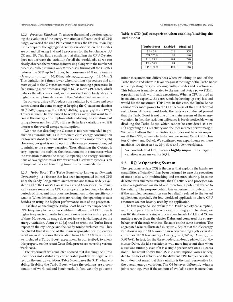
5.2.2 Processes Threshold. To answer the second question regard-

ing the evolution of the energy variation at different levels of CPU

usage, we varied the used PU’s count to track the EV evolution. Fig-

ure 8 compares the aggregated energy variation when the C-states

are on and off using 2, 4 and 8 processes for the benchmarks LU,CG and EP. This figure confirms that disabling the CPU C-states

does not decrease the variation for all the workloads, as we can

clearly observe, the variation is increasing along with the number of

processes. When running only 2 processes, turning off the C-states

reduces the STD up to 6 times, but consumes 20% more energy

(MeanC−states−on = 10, 334mJ , MeanC−states−of f = 12, 594mJ ).This variation is 4 times lower when running 4 processes and al-

most equal to the C-states on mode when running 8 processes. In

fact, running more processes implies to use more CPU cores, which

reduces the idle cores count, so the cores will more likely stay at a

higher consumption state even if the C-states mechanism is on.

In our case, using 4 PU reduces the variation by 4 times and con-

sumes almost the same energy as keeping the C-states mechanism

on (MeanC−states−on = 7, 048mJ ,MeanC−states−of f = 7, 119mJ ).This case would be the closest to reality as we do not want to in-

crease the energy consumption while reducing the variation, but

using a lower number of PU still results in less variation, even if it

increases the overall energy consumption.

We note that disabling the C-states is not recommended in pro-

duction environments, as it introduces extra energy consumption

for low workloads (around 50 % in our case for a single process job).

However, our goal is not to optimize the energy consumption, but

to minimize the energy variation. Thus, disabling the C-states is

very important to stabilize the measurements in some cases when

the variation matters the most. Comparing the energy consump-

tions of two algorithms or two versions of a software systems is an

example of use case benefiting from this recommendation.

5.2.3 Turbo Boost. The Turbo Boost—also known as DynamicOverclocking—is a feature that has been incorporated in Intel CPU

since the Sandy Bridge micro-architecture, and is now widely avail-

able on all of the Core i5, Core i7, Core i9 and Xeon series. It automat-

ically raises some of the CPU cores operating frequency for short

periods of time, and thus boost performances under specific con-

straints. When demanding tasks are running, the operating system

decides on using the highest performance state of the processor.

Disabling or enabling the Turbo Boost has a direct impact on the

CPU frequency behavior, as enabling it allows the CPU to reach

higher frequencies in order to execute some tasks for a short period

of time. However, its usage does not have a trivial impact on the

energy variation. Acun et al. [2] tried to track the Turbo Boost

impact on the Ivy Bridge and the Sandy Bridge architectures. They

concluded that it is one of the main responsible for the energy

variation, as it increases the variation from 1% to 16 %. In our study,

we included a Turbo Boost experiment in our testbed, to check

this property on the recent Xeon Gold processors, covering various

workloads.

The experiment we conducted showed that disabling the Turbo

Boost does not exhibit any considerable positive or negative ef-

fect on the energy variation. Table 3 compares the STD when en-

abling/disabling the Turbo Boost, where the columns are a com-

bination of workload and benchmark. In fact, we only got some

Table 3: STD (mJ) comparison when enabling/disabling the

Turbo Boost

Turbo Boost Enabled Disabled

EP / 5 % 310 308

CG / 25 % 95 140

LU / 25 % 204 240

EP / 50 % 84 79

EP / 100 % 125 110

minor measurements differences when switching on and off the

Turbo Boost, andwhere in favor or against the usage of the Turbo Boost

while repeating tests, considering multiple nodes and benchmarks.

This behavior is mainly related to the thermal design power (TDP),especially at high workloads executions. When a CPU is used at

its maximum capacity, the cores would be heating up very fast and

would hit the maximum TDP limit. In this case, the Turbo Boost

cannot offer more power to the CPU because of the CPU thermal

restrictions. At lower workloads, the tests we conducted proved

that the Turbo Boost is not one of the main reasons of the energy

variation. In fact, the variation difference is barely noticeable when

disabling the Turbo Boost, which cannot be considered as a re-

sult regarding the OS activity and the measurement error margin.

We cannot affirm that the Turbo Boost does not have an impact

on all the CPU, as we only tested on two recent Xeon CPU (clus-

ters Chetemi and Dahu). We confirmed our experiments on these

machines 100 times at 5 %, 25 %, 50 % and 100 % workloads.

We conclude that CPU features highly impact the energy

variation as an answer for RQ 2.

5.3 RQ 3: Operating System

The operating system (OS) is the layer that exploits the hardware

capabilities efficiently. It has been designed to ease the execution

of most tasks with multitasking and resource sharing. In some

delicate tests and measurements, the OS activity and processes can

cause a significant overhead and therefore a potential threat to

the validity. The purpose behind this experiment is to determine

if the sampled consumption can be reliably related to the tested

application, especially for low-workload applications where CPU

resources are not heavily used by the application.

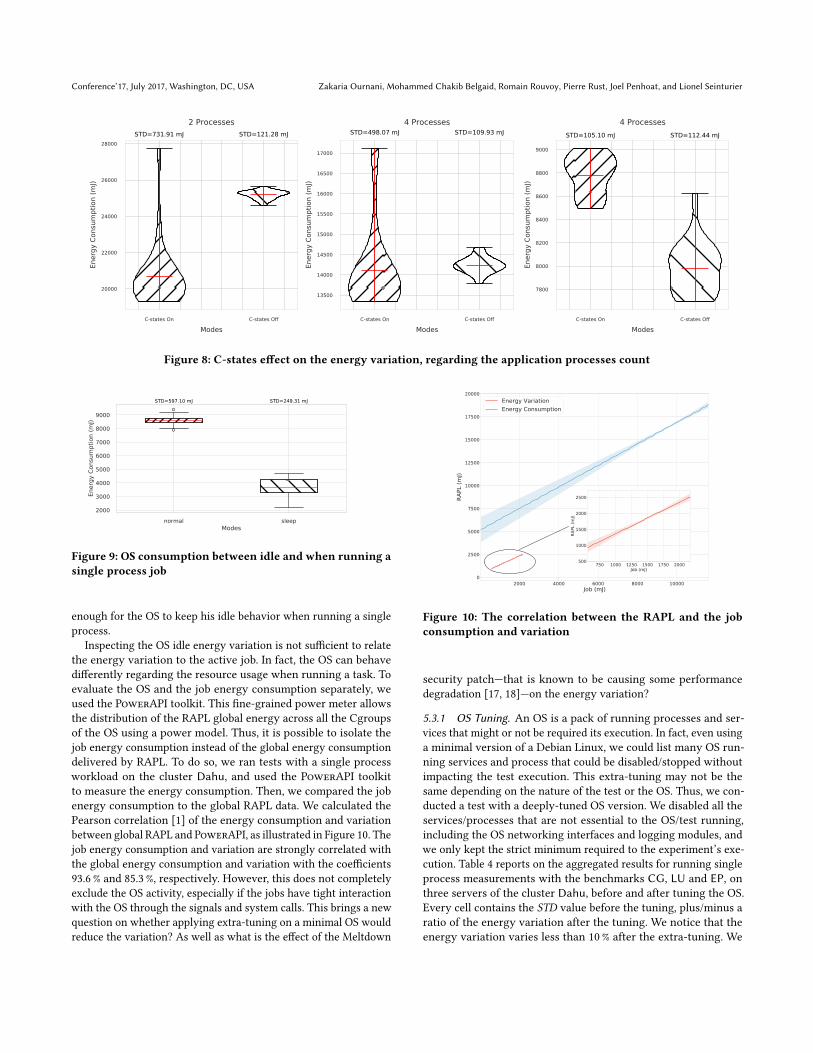
The first way to do is to evaluate theOS idle activity consumption,

and to compare it to a low workload running job. Therefore, we

ran 100 iterations of a single process benchmark EP, LU and CG on

multiple nodes from the cluster Dahu, and compared the energy

behavior of the node with its idle state on the same duration. The

aggregated results, illustrated in Figure 9, depict that the idle energy

variation is up to 140% worst than when running a job, even if it

consumes 120% less energy (Mean Job = 8, 746mJ , MeanIdle =3, 927mJ ). In fact, for the three nodes, randomly picked from the

cluster Dahu, the idle variation is way more important than when

a test was running, even if it is a single process test on a 32-cores

node. This result shows that OS idle consumption varies widely,

due to the lack of activity and the different CPU frequencies states,

but it does not mean that this variation is the main responsible for

the overall energy variation. The OS behaves differently when a

job is running, even if the amount of available cores is more than


C-states On C-states Off

Modes

20000

22000

24000

26000

28000

Ener

gy C

onsu

mpt

ion

(mJ)

STD=731.91 mJ STD=121.28 mJ2 Processes


Modes

13500

14000

14500

15000

15500

16000

16500

17000

Ener

gy C

onsu

mpt

ion

(mJ)



Modes

7800

8000

8200

8400

8600

8800

9000

Ener

gy C

onsu

mpt

ion

(mJ)


Figure 8: C-states effect on the energy variation, regarding the application processes count

normal sleepModes

2000

3000

4000

5000

6000

7000

8000

9000

Ener

gy C

onsu

mpt

ion

(mJ)

STD=249.31 mJSTD=597.10 mJ

singel Process

Figure 9: OS consumption between idle and when running a

single process job

enough for the OS to keep his idle behavior when running a single

process.

Inspecting the OS idle energy variation is not sufficient to relate

the energy variation to the active job. In fact, the OS can behave

differently regarding the resource usage when running a task. To

evaluate the OS and the job energy consumption separately, we

used the PowerAPI toolkit. This fine-grained power meter allows

the distribution of the RAPL global energy across all the Cgroups

of the OS using a power model. Thus, it is possible to isolate the

job energy consumption instead of the global energy consumption

delivered by RAPL. To do so, we ran tests with a single process

workload on the cluster Dahu, and used the PowerAPI toolkit

to measure the energy consumption. Then, we compared the job

energy consumption to the global RAPL data. We calculated the

Pearson correlation [1] of the energy consumption and variation

between global RAPL and PowerAPI, as illustrated in Figure 10. The

job energy consumption and variation are strongly correlated with

the global energy consumption and variation with the coefficients

93.6 % and 85.3 %, respectively. However, this does not completely

exclude the OS activity, especially if the jobs have tight interaction

with the OS through the signals and system calls. This brings a new

question on whether applying extra-tuning on a minimal OS would

reduce the variation? As well as what is the effect of the Meltdown

2000 4000 6000 8000 10000Job (mJ)

0

2500

5000

7500

10000

12500

15000

17500

20000

RAPL

(mJ)

Energy VariationEnergy Consumption

750 1000 1250 1500 1750 2000Job (mJ)

500

1000

1500

2000

2500

RAPL

(mJ)

Figure 10: The correlation between the RAPL and the job

consumption and variation

security patch—that is known to be causing some performance

degradation [17, 18]—on the energy variation?

5.3.1 OS Tuning. An OS is a pack of running processes and ser-

vices that might or not be required its execution. In fact, even using

a minimal version of a Debian Linux, we could list many OS run-

ning services and process that could be disabled/stopped without

impacting the test execution. This extra-tuning may not be the

same depending on the nature of the test or the OS. Thus, we con-

ducted a test with a deeply-tuned OS version. We disabled all the

services/processes that are not essential to the OS/test running,

including the OS networking interfaces and logging modules, and

we only kept the strict minimum required to the experiment’s exe-

cution. Table 4 reports on the aggregated results for running single

process measurements with the benchmarks CG, LU and EP, onthree servers of the cluster Dahu, before and after tuning the OS.

Every cell contains the STD value before the tuning, plus/minus a

ratio of the energy variation after the tuning. We notice that the

energy variation varies less than 10% after the extra-tuning. We


Table 4: STD (mJ) comparison before/after tuning the OS

Node EP CG LU

N1 1370 -9 % 78 +7% 128 +2%

N2 1278 -7 % 64 -1 % 120 +9%

N3 1118 +1% 83 +2% 93 +7%

argue that this variation is not substantial, as it is not stable from

a node to another. Moreover, 10 % of variation is not a representa-

tive difference, due to many factors that can affect it as the CPU

temperature or the measurement errors.

5.3.2 Speculative Executions. Meltdown and Spectre are two of the

most famous hardware vulnerabilities discovered in 2018, and ex-

ploiting them allows a malicious process to access others processes

data that is supposed to be private [17, 18]. They both exploit the

speculative execution technique where a process anticipates some

upcoming tasks, which are not guaranteed to be executed, when

extra resources are available, and revert those changes if not. Some

OS-level patches had been applied to prevent/reduce the criticality

of these vulnerabilities. On the Linux kernel, the patch has been au-

tomatically applied since the version 4.14.12. It mitigates the risk by

isolating the kernel and the user space and preventing the mapping

of most of the kernel memory in the user space. Nikolay et al. havestudied in [21] the impact of patching the OS on the performance.

The results showed that the overall performance decrease is around

2–3 % for most of the benchmarks and real-world applications, only

some specific functions can meet a high performance decrease. In

our study, we are interested in the applied patch’s impact on the

energy variation, as the performance decrease could mean an en-

ergy consumption increase. Thus, we ran the same benchmarks

LU, CG ad EP on the cluster Dahu with different workloads, using

the same OS, with and without the security patch. Table 5 reports

on the STD values before disabling the security patch. A minus

means that the energy varies less without the patch being applied,

while a plus means that it varies more. These results help us to

conclude that the security patch’s effect on the energy variation

is not substantial and can be absorbed through the error margin

for the tested benchmarks. In fact, the best case to consider is the

benchmark LU where the energy variation is less than 10% when

we disable the security patch, but this difference is still moderate.

The little performance difference discussed in [17, 18] may only be

responsible of a small variation, which will be absorbed through

the measurement tools and external noise error margin in most

cases.

Table 5: STD (mJ) comparison with/without the security

patch

Node EP CG LU

N1 269 +2% 83 +1% 108 -6 %

N2 195 +1% 84 -5 % 121 -9 %

N3 223 +/-1 % 72 -4 % 117 +8%

N4 276 +3% 60 +0% 113 -3 %

Table 6: STD (mJ) comparison of experiments from4 clusters

Cluster Dahu Chetemi Ecotype Paranoia

Arch Skylake Broadwell Broadwell Ivy Bridge

Freq 3.7 GHz 3.1 GHz 2.9 GHz 3.0 GHz

TDP 125 W 85 W 55 W 95 W

5% 364 210 75 76

50% 98 86 49 244

100% 119 116 106 240

To answer RQ 3, we conclude that the OS should not be the

main focus of the energy variation taming efforts.

5.4 RQ 4: Processor Generation

Intel microprocessors have noticeably evolved during these last

20 years. Most of the new CPU come with new enhancements to

the chip density, the maximum Frequency or some optimization

features like the C-states or the Turbo Boost. This active evolution

caused that different generations of CPU can handle a task differ-

ently. The aim of this expriment is not to justify the evolution of

the variation across CPU versions/generations, but to observe if the

user can choose the best node to execute her experiments. Previous

papers have discussed the evolution of the energy consumption

variation across CPU generations and concluded that the variation

is getting higher with the latest CPU generations [19, 27], which

makes measurements stability even worse. In this experiment, we

therefore compare four different generations of CPU with the aim

to evaluate the energy variation for each CPU and its correlation

with the generation. Table 6 indicates the characteristics of each of

the tested CPU.

Table 6 also shows the aggregated energy variation of the dif-

ferent generations of nodes for the benchmarks LU, CG and EP.The results attest that the latest versions of CPU do not necessarily

cause more variation. In the experiments we ran, the nodes from

the cluster Paranoia tend to cause more variation at high workloads,

even if they are from the latest generation. While the Skylake CPU

of the clusterDahu cause oftenmore energy variation thanChetemiand the Ecotype Broadwell CPU. We argue that the hypothesis "theenergy consumption on newer CPU varies more" could be true or

not depending on the compared generations, but most importantly,

the chips energy behaviors. On the other hand, our experiments

showed the lowest energy variation when using the Ecotype CPU,these CPU are not the oldest nor the latest, but are tagged with "L"for their low power/TDP. This result rises another hypothesis when

considering CPU choice, which implies selecting the CPU with a

low TDP. This hypothesis has been confirmed on all the Ecotypecluster nodes, especially at low and medium workloads.

Figure 11 is an illustration of the aggregated STD density of

more than 5, 000-random values sets taken from all the conducted

experiments. This shows that the cluster Paranoia reports the worstvariation in most cases, and that Ecotype is the best cluster to

consider to get the least variations, as it has a higher density for

small variation values.

We conclude on affirming RQ 4, as selecting the right CPU

can help to get less variations.


0 50 100 150 200 250STD (mJ)

0.00

0.01

0.02

0.03

0.04

0.05

Rat

e

ChetemiDahuEcotypeParanoia

Figure 11: Energy consumption STD density of the 4 clusters

6 EXPERIMENTAL GUIDELINES

To summarize our experiments, we provide some experimental

guidelines in Table 7, based on the multiple experiments and analy-

sis we did. These guidelines constitute a set ofminimal requirements

or best practices, depending on the workload and the criticality

of the energy measurement precision. It therefore intends to help

practitioners in taming the energy variation on the selected CPU,

and conduct the experiments with the least variations.

Table 7: Experimental Guidelines for Energy Variations

Guideline Load Gain

Use a low TDP CPU Low & medium Up to 3×

Disable the CPU C-states Low Up to 6×

Use the least of sockets in a case of multi-

ple CPU

Medium Up to 30×

Avoid the usage of hyper-threading when-

ever possible

Medium Up to 5×

Avoid rebooting the machine between

tests

High Up to 1.5×

Do not relate to the machine idle variation

to isolate a test EC, the CPU/OS changes

its behavior when a test is running and

can exhibit less variation than idle

Any —

Rather focus the optimization efforts on

the system under test than the OS

Any —

Execute all the similar and comparable ex-

periments on a same machine. Identical

machines can exhibit many differences re-

garding their energy behavior

Any Up to 1.3×

Table 7 gives a proper understanding of known factors, like the

C-states and its variation reduction at low workloads. However, it

also lists some new factors that we identified along the analysis

we conducted in Section 5, such as the results related to the OS or

the reboot mode. Some of the guidelines are more useful/efficient

for specific workloads, as showed in our experiments. Thus, qual-

ifying the workload before conducting the experiments can help

in choosing the proper guidelines to apply. Other studied factors

are not been mentioned in the guidelines, like the Turbo Boost or

the Speculative execution, due to the small effect that has been

observed in our study.

In order to validate the accuracy of our guidelines among a

varied set of benchmarks on one hand, and their effect on the

variation between identical machines on the other hand, we ran

seven experiments with benchmarks and real applications on a

set of four identical nodes from the cluster Dahu, before (normalmode where everything is left to default and to the charge of the

OS) and after (optimized) applying our guidelines. Half of these

experiments has been performed at a 50 % workload and the other

half on single process jobs. The choice of these two workloads is

related to the optimization guidelines that are mainly effective at

low and medium workloads. We note that we used the cluster Dahuover Ecotype to highlight the guidelines effect on the nodes where

the variation is susceptible to be higher.

Figure 12 and 13 highlight the improvement brought by the

adoption of our guidelines. They demonstrate the intra-node STD

reduction at low and medium workloads for all the benchmarks

used at different levels. Concretely, for low workloads, the energy

variation is 2–6 times lower after applying the optimization guide-

lines for the benchmarks LU and EP, as well as Linpack, while itis 1.2–1.8 times better for Sha256. For this workload, the overallenergy consumption after optimization can be up to 80% higher

due to disabling the C-states to keep all the unused cores at a high

power consumption state (MeanLU−normal−Dahu2 = 11, 500mJ ,MeanLU−optimized−Dahu2 = 20, 508mJ ). For medium workloads,

the STD, and thus variation, is up to 100 % better for the benchmark

CG, 20–150% better for the pbzip2 application and up to 100%

for Stress-NG. We note that the optimized version consumes less

energy thanks to an appropriate core pinning method.

Figures 12 and 13 also highlight that applying the guidelines

does not reduce the inter-nodes variation in all the cases. This

variation can be up to 30 % in modern CPU [27]. However, taming

the intra-node variation is a good strategy to identify more relevant

mediums and medians, and then perform accurate comparisons

between the nodes variation. Even though, using the same node

is always better, to avoid the extra inter-nodes variation and thus

improve the stability of measurements.

7 THREATS TO VALIDITY

A number of issues affect the validity of our work. For most of our

experiments, we used the Intel RAPL tool, which has evolved along

Intel CPU generations to be known as one of the most accurate

tools for modern CPU, but still adds an important overhead if we

adopt a sampling at high frequency. The other fine-grained tool

we used for measurements is PowerAPI. It allows to measure the

energy consumption at the granularity of a process or a Cgroup

by dividing the RAPL global energy over the running processes

using a power model. The usage of PowerAPI adds an error margin

because of the power model built over RAPL. The RAPL tool mainly

measures the CPU and DRAM energy consumption. However, even

running CPU/RAM intensive benchmarks would keep a degree

on uncertainty concerning the hard disk and networking energy

consumption. In addition, the operating system adds a layer of

confusion and uncertainty.

The Intel CPU chip manufacturing process and the materials

micro-heterogeneity is one of the biggest issues, as we cannot track

or justify some of the energy variation between identical CPU or


8000

9000

1000

0

1100

0

1200

0

1300

0

1400

0

Energy Consumption (mJ)

norm

alop

timize

dM

odes

STD=227.5 mJ

STD=310.4 mJ

STD=269.4 mJ

STD=254.1 mJ

STD=78.3 mJ

STD=48,9 mJ

STD=187.3 mJ

STD=106.3 mJ

EP Single ProcessDahu30Dahu3Dahu29Dahu25

2000

2250

2500

2750

3000

3250

3500

3750


norm

alop

timize

dM

odes

STD=166.4 mJ

STD=87.2 mJ

STD=125.6 mJ

STD=173.1 mJ

STD=63.0 mJ

STD=56.3 mJ

STD=71.4 mJ

STD=90.2 mJ

CG 50%

Dahu30Dahu3Dahu29Dahu25

1000

0

1200

0

1400

0

1600

0

1800

0

2000

0


norm

alop

timize

dM

odes

STD=422.6 mJSTD=337.5 mJ

STD=559.3 mJ

STD=274.12 mJ

STD=70.9 mJ

STD=82,12 mJ

STD=202.8 mJ

STD=40 mJ

LU Single ProcessDahu18Dahu21Dahu2Dahu31

2500

3000

3500

4000

4500

5000


norm

alop

timize

dM

odes

STD=241.8 mJ

STD=322.5 mJ

STD=291.7 mJ

STD=249.6 mJ

STD=70.5 mJ

STD=64.7 mJ

STD=67.9 mJ

STD=88.6 mJ

Linpack Single Process


1600

1800

2000

2200

2400


norm

alop

timize

dM

odes

STD=118 mJ

STD=78.7 mJ

STD=123.8 mJ

STD=93.1 mJ

STD=88.7 mJ

STD=50.3 mJ

STD=46.6 mJ

STD=85.9 mJ

Pbzip2 50%


200

300

400

500

600

700


norm

alop

timize

dM

odes

STD=81.6 mJ

STD=80.2 mJ

STD=95.6 mJ

STD=94.3 mJ

STD=62.9 mJ

STD=68.4 mJ

STD=52.1 mJ

STD=69.9 mJ

SHA Single Process


Figure 12: Energy variation comparison with/without applying our guidelines

3250 3500 3750 4000 4250 4500 4750


normal

optimized

Mod

es

STD=1133.6 mJ

STD=1089.1 mJ

STD=1087.6 mJ

STD=1086.9 mJ

STD=507.5 mJ

STD=568.9 mJ

STD=554.3 mJ

STD=454.0 mJ

Stress-ng 50%


Figure 13: Energy variation comparison with/without apply-

ing our guidelines for Stress-NG

cores. These CPU/cores might handle frequencies and temperature

differently and behave consequently. This hardware heterogeneity

also makes reproduction complex and requires the usage of the

same nodes on the cluster with the same OS.

8 CONCLUSION

In this paper, we conducted an empirical study of controllable

factors that can increase the energy variations on platforms with

some of the latest CPU, and for several workloads. We provide

a set of guidelines that can be implemented and tuned (through

the OS GRUB for example), especially with the new data centers

isolation trend and the cloud usage, even for scientific and R&D

purposes. Our guidelines aim at helping the user in reducing the

CPU energy variation during systems benchmarking, and conduct

more stable experiments when the variation is critical. For example,

when comparing the energy consumption of two versions of an

algorithm or a software system, where the difference can be tight

and need to be measured accurately.


Overall, our results are not intended to nullify the variability of

the CPU, as some of this variability is related to the chip manufac-

turing process and its thermal behavior. The aim of our work is to

be able to tame and mitigate this variability along controlled ex-

periments. We studied some previously discussed aspects on some

recent CPU, considered new factors that have not been deeply

analyzed to the best of our knowledge, and constituted a set of

guidelines to achieve the variability mitigating purpose. Some of

these factors, like the C-states usage, can reduce the energy vari-

ation up to 500% at low workloads, while choosing the wrong

cores/PU strategy can cause up to 30× more variability.

We believe that our approach can also be used to study/discover

other potential variability factors, and extend our results to alterna-

tive CPU generations/brands. Most importantly, this should moti-

vate future works on creating a better knowledge on the variability

due to CPU manufacturing process and other factors.

REFERENCES

[1] 2008. Pearson’s Correlation Coefficient. Springer Netherlands.[2] Bilge Acun, Phil Miller, and Laxmikant V. Kale. 2016. Variation Among Processors

Under Turbo Boost in HPC Systems. (2016).

[3] D. H. Bailey, E. Barszcz, J. T. Barton, D. S. Browning, R. L. Carter, L. Dagum,

R. A. Fatoohi, P. O. Frederickson, T. A. Lasinski, R. S. Schreiber, H. D. Simon,

V. Venkatakrishnan, and S. K. Weeratunga. 1991. The NAS Parallel Bench-

marks&Mdash;Summary and Preliminary Results. (1991).

[4] Daniel Balouek, Alexandra Carpen Amarie, Ghislain Charrier, Frédéric Desprez,

Emmanuel Jeannot, Emmanuel Jeanvoine, Adrien Lèbre, David Margery, Nicolas

Niclausse, Lucas Nussbaum, Olivier Richard, Christian Pérez, Flavien Quesnel,

Cyril Rohr, and Luc Sarzyniec. 2013. Adding Virtualization Capabilities to the

Grid’5000 Testbed. In Cloud Computing and Services Science. Communications in

Computer and Information Science, Vol. 367. Springer.

[5] S. Borkar. 2005. Designing Reliable Systems from Unreliable Components: The

Challenges of Transistor Variability and Degradation. IEEE Micro 25, 6 (Nov.

2005).

[6] Dimitrios Chasapis, Martin Schulz, Marc Casas, Eduard Ayguadé, Mateo Valero,

Miquel Moretó, and Jesus Labarta. 2016. Runtime-Guided Mitigation of Manufac-

turing Variability in Power-Constrained Multi-Socket NUMA Nodes. (2016).

[7] Henry Coles, Yong Qin, and Phillip Price. 2014. Comparing Server Energy Use andEfficiency Using Small Sample Sizes. Technical Report LBNL-6831E, 1163229.

[8] Maxime Colmant, Romain Rouvoy, Mascha Kurpicz, Anita Sobe, Pascal Felber,

and Lionel Seinturier. 2018. The next 700 CPU power models. Journal of Systemsand Software 144 (2018).

[9] Eddie Antonio Santos, Carson McLean, Christophr Solinas, and Abram Hindle.

2017. How Does Docker Affect Energy Consumption? Evaluating Workloads in

and out of Docker Containers. The journal of systems & Software (2017).[10] Bradley Efron. 2000. The bootstrap and modern statistics. J. Amer. Statist. Assoc.

95, 452 (2000).

[11] Mohammed El Mehdi Diouri, Olivier Gluck, Laurent Lefevre, and Jean-Christophe

Mignot. 2013. Your Cluster Is Not Power Homogeneous: Take Care When De-

signing Green Schedulers! (June 2013).

[12] Adam Hammouda, Andrew R. Siegel, and Stephen F. Siegel. 2015. Noise-Tolerant

Explicit Stencil Computations for Nonuniform Process Execution Rates. ACMTransactions on Parallel Computing 2, 1 (April 2015).

[13] Franz Heinrich, Alexandra Carpen-Amarie, Augustin Degomme, Sascha Hunold,

Arnaud Legrand, Anne-Cécile Orgerie, and Martin Quinson. 2017. Predicting the

Performance and the Power Consumption of MPI Applications With SimGrid.

(2017).

[14] Yuichi Inadomi, Masatsugu Ueda, Masaaki Kondo, Ikuo Miyoshi, Tapasya Patki,

Koji Inoue, Mutsumi Aoyagi, Barry Rountree, Martin Schulz, David Lowenthal,

Yasutaka Wada, and Keiichiro Fukazawa. 2015. Analyzing and Mitigating the

Impact of Manufacturing Variability in Power-Constrained Supercomputing.

(2015).

[15] Joakim v Kisroski, Hansfreid Block, John Beckett, Cloyce Spradling, Klaus-Dieter

Lange, and Samuel Kounev. 2016. Variations in CPU Power Consumption. (March

2016).

[16] Kashif Nizam Khan, Mikael Hirki, Tapio Niemi, Jukka K. Nurminen, and

Zhonghong Ou. 2018. RAPL in Action: Experiences in Using RAPL for Power

Measurements. ACM Trans. Model. Perform. Eval. Comput. Syst. 3, 2, Article 9(March 2018).

[17] Paul Kocher, Jann Horn, Anders Fogh, , Daniel Genkin, Daniel Gruss, Werner

Haas, Mike Hamburg, Moritz Lipp, Stefan Mangard, Thomas Prescher, Michael

Schwarz, and Yuval Yarom. 2019. Spectre Attacks: Exploiting Speculative Execu-

tion. (2019).

[18] Moritz Lipp, Michael Schwarz, Daniel Gruss, Thomas Prescher, Werner Haas,

Anders Fogh, Jann Horn, Stefan Mangard, Paul Kocher, Daniel Genkin, Yuval

Yarom, and Mike Hamburg. 2018. Meltdown: Reading Kernel Memory from User

Space. (2018).

[19] Aniruddha Marathe, Yijia Zhang, Grayson Blanks, Nirmal Kumbhare, Ghaleb

Abdulla, and Barry Rountree. 2017. An Empirical Survey of Performance and

Energy Efficiency Variation on Intel Processors. (2017).

[20] David Margery, Emile Morel, Lucas Nussbaum, Olivier Richard, and Cyril Rohr.

2014. Resources Description, Selection, Reservation and Verification on a Large-

scale Testbed. (May 2014).

[21] Nikolay A. Simakov, Martins D. Innus, Matthew D. Jones, Joseph P. White,

Steven M. Gallo, Robert L. DeLeon, and Thomas R. FOPTurlani. 2018. Effect of

Meltdown and Spectre Patches on the Performance of HPC Applications. CoRRabs/1801.04329 (2018). arXiv:1801.04329

[22] J.W. Tschanz, J.T. Kao, S.G. Narendra, R. Nair, D.A. Antoniadis, A.P. Chandrakasan,

and V. De. 2002. Adaptive Body Bias for Reducing Impacts of Die-to-Die and

within-Die Parameter Variations on Microprocessor Frequency and Leakage.

IEEE Journal of Solid-State Circuits 37, 11 (Nov. 2002).[23] Erik van der Kouwe, Dennis Andriesse, Herbert Bos, Cristiano Giuffrida, and

Gernot Heiser. 2018. Benchmarking Crimes: An Emerging Threat in Systems

Security. CoRR abs/1801.02381 (2018). arXiv:1801.02381

[24] Georgios Varsamopoulos, Ayan Banerjee, and Sandeep K. S. Gupta. 2009. Energy

Efficiency of Thermal-Aware Job Scheduling Algorithms under Various Cooling

Models. In Contemporary Computing. Vol. 40. Springer.[25] A. Vasan, A. Sivasubramaniam, V. Shimpi, T. Sivabalan, and R. Subbiah. 2010.

Worth their watts? - an empirical study of datacenter servers. (Jan 2010).

[26] Yewan Wang, David Nörtershäuser, Stéphane Le Masson, and Jean-Marc Menaud.

2018. Potential Effects on Server PowerMetering andModeling.Wireless Networks(Nov. 2018).

[27] Yewan Wang, David Nörtershäuser, Stéphane Le Masson, and Jean-Marc Menaud.

[n. d.]. Experimental Characterization of Variation in Power Consumption for

Processors of Different Generations. ([n. d.]).

http://arxiv.org/abs/1801.04329

http://arxiv.org/abs/1801.02381

taming energy consumption variations in systems benchmarking

Documents