Provable and Practical Approximations for the DegreeDistribution using Sublinear Graph Samples∗

Talya EdenSchool of Computer Science, Tel Aviv

UniversityTel Aviv, Israel

talyaa01@gmail.com

Shweta JainUniversity of California, Santa Cruz

Santa Cruz, CA, USAsjain12@ucsc.edu

Ali PinarSandia National Laboratories

Livermore, CAapinar@sandia.gov

Dana RonSchool of Computer Science, Tel Aviv

UniversityTel Aviv, Israel

danaron@tau.ac.il

C. SeshadhriUniversity of California, Santa Cruz

Santa Cruz, CAsesh@ucsc.edu

ABSTRACTThe degree distribution is one of the most fundamental propertiesused in the analysis of massive graphs. There is a large literature ongraph sampling, where the goal is to estimate properties (especiallythe degree distribution) of a large graph through a small, randomsample. Estimating the degree distribution of real-world graphsposes a significant challenge, due to their heavy-tailed nature andthe large variance in degrees.

We design a new algorithm, SADDLES, for this problem,using recent mathematical techniques from the field of sublinearalgorithms. The SADDLES algorithm gives provably accurateoutputs for all values of the degree distribution. For the analysis,we define two fatness measures of the degree distribution, calledthe h-index and the z-index. We prove that SADDLES is sublinearin the graph size when these indices are large. A corollary of thisresult is a provably sublinear algorithm for any degree distributionbounded below by a power law.

We deploy our new algorithm on a variety of real datasets anddemonstrate its excellent empirical behavior. In all instances, weget extremely accurate approximations for all values in the degreedistribution by observing at most 1% of the vertices. This is a majorimprovement over the state-of-the-art sampling algorithms, whichtypically sample more than 10% of the vertices to give comparableresults. We also observe that the h and z-indices of real graphs arelarge, validating our theoretical analysis.

ACM Reference Format:Talya Eden, Shweta Jain, Ali Pinar, Dana Ron, and C. Seshadhri. 2018.Provable and Practical Approximations for the Degree Distribution usingSublinear Graph Samples. In Proceedings of ACM Conference (Conference’17).

∗Both Talya Eden and Shweta Jain contributed equally to this work, and are joint firstauthors of this work.

Permission to make digital or hard copies of part or all of this work for personal orclassroom use is granted without fee provided that copies are not made or distributedfor profit or commercial advantage and that copies bear this notice and the full citationon the first page. Copyrights for third-party components of this work must be honored.For all other uses, contact the owner/author(s).Conference’17, July 2017, Washington, DC, USA© 2018 Copyright held by the owner/author(s).ACM ISBN 978-x-xxxx-xxxx-x/YY/MM.https://doi.org/10.1145/nnnnnnn.nnnnnnn

ACM, New York, NY, USA, 11 pages. https://doi.org/10.1145/nnnnnnn.nnnnnnn

1 INTRODUCTIONIn domains as diverse as social sciences, biology, physics,cybersecurity, graphs are used to represent entities and therelationships between them. This has led to the explosive growthof network science as a discipline over the past decade. One ofthe hallmarks of network science is the occurrence of specificgraph properties that are common to varying domains, such asheavy tailed degree distributions, large clustering coefficients,and small-world behavior. Arguably, the most significant amongthese properties is the degree distribution, whose study led to thefoundation of network science [7, 8, 20].

Given an undirected graph G, the degree distribution (ortechnically, histogram) is the sequence of numbers n(1),n(2), . . .,where n(d) is the number of vertices of degree d . In almost allreal-world scenarios, the average degree is small, but the variance(and higher moments) is large. Even for relatively large d , n(d)is still non-zero, and n(d) typically has a smooth non-increasingbehavior. In Fig. 1, we see the typical degree distribution behavior.The average degree in a Google web network is less than 10, butthe maximum degree is more than 5000. There are also numerousvertices with all intermediate degrees. This is referred to as a “heavytailed" distribution. The degree distribution, especially the tail, isof significant relevance to modeling networks, determining theirresilience, spread of information, and for algorithmics [6, 9, 13, 16,33–36, 42].

With full access to G, the degree distribution can be computedin linear time, by simply determining the degree of each vertex.Yet in many scenarios, we only have partial access to the graph,provided through some graph samples. A naive extrapolation ofthe degree distribution can result in biased results. The seminalresearch paper of Faloutsos et al. claimed a power law in the degreedistribution on the Internet [20]. This degree distribution wasdeduced by measuring a power law distribution in the graph samplegenerated by a collection of traceroute queries on a set of routers.Unfortunately, it was mathematically and empirically proven thattraceroute responses can have a power law even if the true network

arX

iv:1

710.

0860

7v3

[cs

.SI]

28

Aug

201

8

does not [1, 11, 27, 37]. In general, a direct extrapolation of thedegree distribution from a graph subsample is not valid for theunderlying graph. This leads to the primary question behind ourwork.

How can we provably and practically estimate the degreedistribution without seeing the entire graph?

There is a rich literature in statistics, data mining, and physicson estimating graph properties (especially the degree distribution)using a small subsample [2, 3, 5, 17, 28, 30, 31, 39, 46, 47].Nonetheless, there is no provable algorithm for the entire degreedistribution, with a formal analysis on when it is sublinear in thenumber of vertices. Furthermore, most empirical studies typicallysample 10-30% of the vertices for reasonable estimates.

1.1 Problem descriptionWe focus on the complementary cumulative degree histogram (oftencalled the cumulative degree distribution) or ccdh of G. This isthe sequence N (d), where N (d) = ∑

r ≥d n(r ) is the number ofvertices of degree at least d . The ccdh is typically used for fittingdistributions, since it averages out noise and is monotonic [12]. Ouraim is to get an accurate bicriteria approximation to the ccdh ofG,at all values of d .

Definition 1.1. The sequence N (d) is an (ε, ε)-estimate of theccdh if ∀d , (1 − ε)N ((1 + ε)d) ≤ N (d) ≤ (1 + ε)N ((1 − ε)d).

Computing an (ε, ε)-estimate is significantly harder thanapproximating the ccdh using standard distribution measures.Statistical measures, such as the KS-distance, χ2, ℓp -norms, etc.tend to ignore the tail, since (in terms of probability mass) it is anegligible portion of the distribution. An (ε, ε)-estimate is accuratefor all d .

The query model: A formal approach requires specifying aquery model for accessing G. We look to the subfields of propertytesting and sublinear algorithms within theoretical computerscience for such models [22, 23]. Consider the following three kindsof queries.

• Vertex queries: acquire a uniform random vertex v ∈ V .• Neighbor queries: given v ∈ V , acquire a uniform random

neighbor u of V .• Degree queries: given v ∈ V , acquire the degree dv .

An algorithm is only allowed to make these queries to process theinput. It has to make some number of queries, and finally producean output. We discuss two query models, and give results for both.

The Standard Model (SM) All queries allowed: This is thestandardmodel in numerous sublinear algorithms results [18, 19, 22–24]. Furthermore, most papers on graph sampling implicitly use thismodel for generating subsamples. Indeed, any method involvingcrawling from a random set of vertices and collecting degrees is inthe SM. This model is the primary setting for our work, and allowsfor comparison with rich body of graph sampling algorithms. It isworth noting that in the SM, one can determine the entire degreedistribution inO(n logn) queries (the extra logn factor comes fromthe coupon collector bound of finding all the vertices throughuniform sampling). Thus, it makes sense to express the number ofqueries made by an algorithm as a fraction of n. Alternately, the

number of queries is basically the number of vertices encounteredby the algorithm. Thus, a sublinear algorithm makes o(n) queries.

The Hidden Degrees Model (HDM) Vertex and neighborqueries allowed, not degree queries: This is a substantially weakermodel. In numerous cybersecurity and network monitoringsettings, an algorithm cannot query for degrees, and has to inferthem indirectly. Observe that this model is significantly harderthan the SM. It takes O((m + n) logn) to determine all the degrees,since one has to at least visit all the edges to find degrees exactly.In this model, we express the number of queries as a fraction ofm.

Regarding uniform random vertex queries: This is a fairlypowerful query, that may not be realizable in all situations. Indeed,Chierichetti et al. explicitly study this problem in social networksand design (non-trivial) algorithms for sampling uniform randomvertices [10]. In a previous work, Dasgupta, Kumar, and Sarlosstudy algorithms for estimating average degree when only randomwalks are possible [14]. Despite this power, we believe that SM isa good testbed for understanding when a small sample of a graphprovably gives properties of the whole. Furthermore, in the contextof graph sampling, access to uniform random vertices is commonly(implicitly) assumed [5, 17, 28, 30, 38, 39, 47]. The vast majority ofexperiments conducted often use uniform random vertices.

As a future direction, we believe it is important to investigatesampling models without random vertex queries.

1.2 Our contributionsOur main theoretical result is a new sampling algorithm, theSublinear Approximations for Degree Distributions LeveragingEdge Samples, or SADDLES. This algorithm provably provides(ε, ε)-approximations for the ccdh. We show how to designSADDLES under both the SM and the HDM.We apply SADDLES ona variety of real datasets and demonstrate its ability to accuratelyapproximate the ccdh with a tiny sample of the graph.

• Sampling algorithm for estimating ccdh: Our algorithmcombines a number of techniques in random sampling to get(ε, ε)-estimates for the ccdh. A crucial component is an applicationof an edge simulation technique, first devised by Eden et al. in thecontext of triangle counting [18, 19]. This (theoretical) techniqueshows how to get a collection of weakly correlated uniform randomedges from independent uniform vertices. SADDLES employs aweighting scheme on top of this method to estimate the ccdh.

• Heavy tails leads to sublinear algorithms: The challengein analyzing SADDLES is in finding parameters of the ccdh thatallow for sublinear query complexity. To that end, we discuss twoparameters that measure “heaviness" of the distribution tail: theclassich-index and a newly defined z-index.We prove that the querycomplexity of SADDLES is sublinear (for both models) wheneverthese indices are large.

• Excellent empirical behavior: We deploy animplementation of SADDLES on a collection of large real-worldgraphs. In all instances, we achieve extremely accurate estimatesfor the entire ccdh by sampling at most 1% of the vertices of thegraph. Refer to Fig. 1. Observe how SADDLES tracks various jumpsin the ccdh, for all graphs in Fig. 1.

• Comparison with existing samplingmethods: A numberof graph sampling methods have been proposed in practice, such

2

(a) amazon0601 copurchase network (b) web-Google web network (c) cit-Patents citation network (d) com-orkut social network

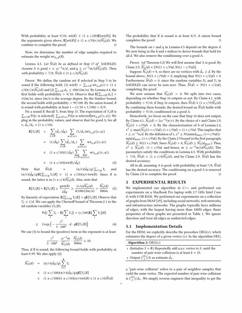
Figure 1: The output of SADDLES on a collection of networks: amazon0601 (403K vertices, 4.9M edges), web-Google (870K vertices,4.3M edges), cit-Patents (3.8M vertices, 16M edges), com-orkut social network (3M vertices, 117M edges). SADDLES samples 1%of the vertices and gives accurate results for the entire (cumulative) degree distribution. For comparison, we show the outputof a number of sampling algorithms from past work, each run with the same number of samples. (Because of the size ofcom-Orkut, methods involving optimization [47] fail to produce an estimate in reasonable time.)

as vertex sampling (VS), snowball sampling (OWS), forest-firesampling (FF), induced graph sampling (IN), random walk (RWJ),edge sampling (ES) [5, 17, 28, 30, 38, 39, 47]. A recent work of Zhanget al. explicitly addresses biases in these sampling methods, andfixes them using optimization techniques [47].We run head-to-headcomparisons with all these sampling methods, and demonstrate theSADDLES gives significantly better practical performance. Fig. 1shows the output of all these sampling methods with a total samplesize of 1% of the vertices. Observe how across the board, themethodsmake erroneous estimates for most of the degree distribution. Theerrors are also very large, for all the methods. This is consistentwith previous work, where methods sample more than 10% of thenumber of vertices.

1.3 Theoretical results in detailOur main theoretical result is a new sampling algorithm, theSublinear Approximations for Degree Distributions LeveragingEdge Samples, or SADDLES.

We first demonstrate our results for power law degreedistributions [7, 8, 20]. Statistical fitting procedures suggest theyoccur to some extent in the real-world, albeit with much noise [12].The classic power law degree distribution sets n(d) ∝ 1/dγ , whereγ is typically in [2, 3]. We build on this to define a power law lowerbound.

Definition 1.2. Fix γ > 2. A degree distribution is bounded belowby a power law with exponent γ , if the ccdh satisfies the followingproperty. There exists a constant τ > 0 such that for all d , N (d) ≥⌊τn/dγ−1⌋.

The following is a corollary of our main result. For convenience,we will suppress query complexity dependencies on ε and lognfactors, using O(·).

Theorem 1.3. Suppose the degree distribution of G is boundedbelow by a power law with exponent γ . Let the average degree bedenoted by d . For any ε > 0, the SADDLES algorithm outputs (with

high probability) an (ε, ε)-approximation to the ccdh and makes thefollowing number of queries.

• SM: O(n1−1γ + n

1− 1γ −1d)

• HDM: O(n1−1

2(γ −1)d)

In most real-world instances, the average degree d is typicallyconstant. Thus, the complexities above are strongly sublinear. Forexample, when γ = 2, we get O(n1/2) for both models. When γ = 3,we get O(n2/3) and O(n3/4).

Our main result is more nuanced, and holds for all degreedistributions. If the ccdh has a heavy tail, we expect N (d) tobe reasonably large even for large values of d . We describe twoformalisms of this notion, through fatness indices.

Definition 1.4. The h-index of the degree distribution is thelargest d such that there are at least d vertices of degree at least d .

This is the exact analogy of the bibliometric h-index [26]. As weshow in the §2.1, h can be approximated by mind (d + N (d))/2. Amore stringent index is obtained by replacing the arithmetic meanby the (smaller) geometric mean.

Definition 1.5. The z-index of the degree distribution is z =mind :N (d )>0

√d · N (d).

Our main theorem asserts that large h and z indices lead to asublinear algorithm for degree distribution estimation. Theorem 1.3is a direct corollary obtained by plugging in values of the indicesfor power laws.

Theorem 1.6. For any ε > 0, the SADDLES algorithm outputs(with high probability) an (ε, ε)-approximation to the ccdh, and makesthe following number of queries.

• SM: O(n/h +m/z2)• HDM: O(m/z)

1.4 Challenges and Main IdeaThe heavy-tailed behavior of the real degree distribution posesthe primary challenge to computing (ε, ε)-estimates to the ccdh.

3

As d increases, there are fewer and fewer vertices of that degree.Sampling uniform random vertices is inefficient when N (d) is small.A natural idea to find high degree vertices to pick a randomneighborof a random vertex. Such a sample is more likely to be a high degreevertex. This is the idea behind methods like snowball sampling,forest fire sampling, randomwalk sampling, graph sample-and-hold,etc. [5, 17, 28, 30, 38, 39, 47]. But these lead to biased samples,since vertices with the same degree may be picked with differingprobabilities.

A direct extrapolation/scaling of the degrees in the observedgraph does not provide an accurate estimate. Our experimentsshow that existing methods always miss the head or the tail. A moreprincipled approach was proposed recently by Zhang et al. [47],by casting the estimation of the unseen portion of the distributionas an optimization problem. From a mathematical standpoint, thevast majority of existing results tend to analyze the KS-statistic, orsome ℓp -norm. As we mentioned earlier, this does not work wellfor measuring the quality of the estimate at all scales. As shown byour experiments, none of these methods give accurate estimate forthe entire ccdh with less than 5% of the vertices.

The main innovation in SADDLES comes through the use ofa recent theoretical technique to simulate edge samples throughvertex samples [18, 19]. The sampling of edges occurs throughtwo stages. In the first stage, the algorithm samples a set of rvertices and sets up a distribution over the sampled vertices suchthat any edge adjacent to a sampled vertex may be sampled withuniform probability. In the second stage, it samples q edges fromthis distribution. While a single edge is uniform random, the set ofedges are correlated.

For a given d , we define a weight function on the edges, suchthat the total weight is exactly N (d). SADDLES estimates the totalweight by scaling up the average weight on a random sample ofedges, generated as discussed above. The difficulty in the analysisis the correlation between the edges. Our main insight is that if thedegree distribution has a fat tail, this correlation can be containedeven for sublinear r and q. Formally, this is achieved by relating theconcentration behavior of the average weight of the sample to theh and z-indices. The final algorithm combines this idea with vertexsampling to get accurate estimates for all d .

The hidden degrees model is dealt with using birthday paradoxtechniques formalized by Ron and Tsur [41]. It is possible toestimate the degree dv using O(

√dv ) neighbor queries. But this

adds overhead to the algorithm, especially for estimating the ccdhat the tail. As discussed earlier, we need methods that bias towardshigher degrees, but this significantly adds to the query cost ofactually estimating the degrees.

1.5 Related WorkThere is a rich body of literature on generating a graph samplethat reveals graph properties of the larger “true" graph. We donot attempt to fully survey this literature, and only refer toresults directly related to our work. The works of Leskovec &Faloutsos [30], Maiya & Berger-Wolf [31], and Ahmed, Neville,& Kompella [2, 5] provide excellent surveys of multiple samplingmethods.

There are a number of sampling methods based on randomcrawls: forest-fire [30], snowball sampling [31], and expansionsampling [30]. As has been detailed in previous work, thesemethodstend to bias certain parts of the network, which can be exploited formore accurate estimates of various properties [30, 31, 39]. A seriesof papers by Ahmed, Neville, and Kompella [2–5] have proposedalternate sampling methods that combine random vertices andedges to get better representative samples.

All these results aim to capture numerous properties of the graph,using a single graph sample. Nonetheless, there is much previouswork focused on the degree distribution. Ribiero and Towsley [39]and Stumpf and Wiuf [46] specifically study degree distributions.Ribiero and Towsley [39] do detailed analysis on degree distributionestimates (they also look at the ccdh) for a variety of these samplingmethods. Their empirical results show significant errors either atthe head or the tail. We note that almost all these results end upsampling up to 20% of the graph to estimate the degree distribution.

Zhang et al. observe that the degree distribution of numeroussampling methods is a random linear projection of the truedistribution [47]. They attempt to invert this (ill-conditioned) linearproblem, to correct the biases. This leads to improvement in theestimate, but the empirical studies typically sample more than 10%of the vertices for good estimates.

A recent line of work by Soundarajan et al. on active probingalso has flavors of graph sampling [44, 45]. In this setting, we startwith a small, arbitrary subgraph and try to grow this subgraphto achieve some coverage objective (like discover the maximumnew vertices, find new edges, etc.). The probing schemes devisedin these papers outperform uniform random sampling methods forcoverage objectives.

Some methods try to match the shape/family of the distribution,rather than estimate it as a whole [46]. Thus, statistical methodscan be used to estimate parameters of the distribution. But it isreasonably well-established that real-world degree distributionsare rarely pure power laws in most instances [12]. Indeed, fittinga power law is rather challenging and naive regression fits onlog-log plots are erroneous, as results of Clauset-Shalizi-Newmanshowed [12].

The subfield of property testing and sublinear algorithms for sparsegraphs within theoretical computer science can be thought of asa formalization of graph sampling to estimate properties. Indeed,our description of the main problem follows this language. Thereis a very rich body of mathematical work in this area (refer toRon’s survey [40]). Practical applications of graph property testingare quite rare, and we are only aware of one previous work onapplications for finding dense cores in router networks [25]. Thespecific problem of estimating the average degree (or the totalnumber of edges) was studied by Feige [21] and Goldreich-Ron [23].Gonen et al. and Eden et al. focus on the problem of estimatinghigher moments of the degree distribution [19, 24]. One of the maintechniques we use of simulating edge queries was developed insublinear algorithms results of Eden et al. [18, 19] in the context oftriangle counting and degree moment estimation. We stress that allthese results are purely theoretical, and their practicality is by nomeans obvious.

On the practical side, Dasgupta, Kumar, and Sarlos studyaverage degree estimation in real graphs, and develop alternate

4

algorithms [14]. They require the graph to have low mixingtime and demonstrate that the algorithm has excellent behaviorin practice (compared to implementations of Feige’s and theGoldreich-Ron algorithm [21, 23]). Dasgupta et al. note thatsampling uniform random vertices is not possible in many settings,and thus they consider a significantly weaker setting than SM orHDM. Chierichetti et al. focus on sampling uniform random vertices,using only a small set of seed vertices and neighbor queries [10].

We note that there is a large body of work on sampling graphsfrom a stream [32]. This is quite different from our setting, sincea streaming algorithm observes every edge at least once. Thespecific problem of estimating the degree distribution at all scaleswas considered by Simpson et al. [43]. They observe many of thechallenges we mentioned earlier: the difficulty of estimating thetail accurately, finding vertices at all degree scales, and combiningestimates from the head and the tail.

2 PRELIMINARIESWe say that the input graph G has n vertices and m edges andm ≥ n (since isolated vertices are not relevant here). For any vertexv , let Γ(v) be the neighborhood of v , and dv be the degree. Asmentioned earlier, n(d) is the number of vertices of degree d andN (d) = ∑

r ≥d n(r ) is the ccdh at d . We use “u.a.r." as a shorthand for“uniform at random". We stress that the all mention of probabilityand error is with respect to the randomness of the samplingalgorithm. There is no stochastic assumption on the input graph G .We use the shorthand A ∈ (1± α)B for A ∈ [(1− α)B, (1+ α)B]. Wewill apply the following (rescaled) Chernoff bound.

Theorem 2.1. [Theorem 1 in [15]] Let X1,X2, . . . ,Xk be asequence of iid random variables with expectation µ. Furthermore,Xi ∈ [0,B].

• For ε < 1, Pr[|∑ki=1 Xi − µk | ≥ εµk] ≤ 2 exp(−ε2µk/3B).

• For t ≥ 2eµ, Pr[∑ki=1 Xi ≥ tk] ≤ 2−tk/B .

2.1 More on Fatness indicesThe following characterization of the h-index will be useful foranalysis. Since (d+N (d))/2 ≤ max(d,N (d)) ≤ d+N (d), this provesthat mind (d + N (d))/2 is a 2-factor approximation to the h-index.

Lemma 2.2. mind max(d,N (d)) ∈ h,h + 1

Proof. Let s = mind max(d,N (d)) and let the minimumbe attained at d∗. If there are multiple minima, let d∗ be thelargest among them. We consider two cases. (Note that N (d) isa monotonically non-increasing sequence.)

Case 1: N (d∗) ≥ d∗. So s = N (d∗). Since d∗ is the largestminimum, for any d > d∗, d > N (d∗). (If not, then the minimum isalso attained at d > d∗.) Thus, d > N (d∗) ≥ N (d). For any d < d∗,N (d) ≥ N (d∗) ≥ d∗ > d . We conclude that d∗ is largest d such thatN (d) ≥ d . Thus, h = d∗.

If s , h, then d∗ < N (d∗). Then, N (d∗ + 1) < N (d∗), otherwisethe minimum would be attained at d∗ + 1. Furthermore, max(d∗ +1,N (d∗ + 1)) > N (d∗), implying d∗ + 1 > N (d∗). This proves thath + 1 > s .

Case 2: d∗ > N (d∗). So s = d∗. For d > d∗, N (d) ≤ N (d∗) < d∗ <d . For d < d∗, N (d) ≥ d∗ > d (if N (d) < d∗, then d∗ would not be

the minimizer). Thus, d∗ − 1 is the largest d such that N (d) ≥ d ,and h = d∗ − 1 = s − 1.

The h-index does not measure d vs N (d) at different scales, anda large h-index only ensures that there are “enough” high-degreevertices. For instance, the h-index does not distinguish betweentwo different distributions whose ccdh N1 and N2 are such thatN1(100) = 100 and N1(d) = 0 for d > 100, and N2(100, 000) = 100and N2(d) = 100 for all other values of d ≥ 100. The h-index inboth these cases is 100.

The h and z-indices are related to each other.

Claim 2.3.√h ≤ z ≤ h.

Proof. Since N (d) is integral, if N (d) > 0, then N (d) ≥ 1. Thus,for all N (d) > 0,

√max(d,N (d)) ≤ d · N (d) ≤ max(d,N (d)). We

take the minimum over all d to complete the proof.

To give some intuition about these indices, we compute theh andz index for power laws. The classic power law degree distributionsets n(d) ∝ 1/dγ , where γ is typically in [2, 3].

Claim 2.4. If a degree distribution is bounded below by a power

law with exponent γ , then h = Ω(n1γ ) and z = Ω(n

12(γ −1) ).

Proof. Consider d ≤ τn1/γ , where τ is defined according toDefinition 1.2. Then, N (d) ≥ ⌊τn/(τ 1/γn(γ−1)/γ )⌋ = Ω(n1/γ ). Thisproves the h-index bound.

Set d∗ = (τn)1

γ −1 . For d ≤ d∗, N (d) ≥ 1 and d · N (d) ≥(τ/2)n/dγ−2 = Ω(n

1γ −1 ). If there exists no d > d∗ such that

N (d) > 0, then z = Ω(n1

2(γ −1) ). If there does exist some such d ,then z = Ω(

√d∗) which yields the same value.

Plugging in values, for γ = 2, both h and z are Ω(√n). For γ = 3,

h = Θ(n1/3) and z = Θ(n1/4).

2.2 Simulating degree queries for HDMThe Hidden Degrees Model does not allow for querying the degreedv of a vertexv . Nonetheless, it is possible to get accurate estimatesof dv by sampling u.a.r. neighbors (with replacement) of v . Thiscan be done by using the birthday paradox argument, as formalizedby Ron and Tsur [41]. Roughly speaking, one repeatedly samplesneighbors until the same vertex is seen twice. If this happens after tsamples, t2 is a constant factor approximation fordv . This argumentcan be refined to get accurate approximations for dv usingO(

√dv )

random edge queries.

Theorem 2.5. [Theorem 3.1 of [41], restated] Fix any α > 0. Thereis an algorithm that outputs a value in (1 ± α)dv with probability> 2/3, and makes an expected O(

√dv/α2) u.a.r. neighbor samples.

For the sake of the theoretical analysis, we will simply assumethis theorem. In the actual implementation of SADDLES, we willdiscuss the specific parameters used. It will be helpful to abstractout the estimation of degrees through the following corollary. Theprocedure DEG(v) will be repeatedly invoked by SADDLES. This isa direct consequence of setting α − ε/10 and applying Theorem ??with δ = 1/n3.

5

Corollary 2.6. There is an algorithm DEG that takes as input avertex v , and has the following properties:

• For all v : with probability > 1 − 1/n3, the output DEG(v) is in(1 ± ε/10)dv .

• The expected running time and query complexity of DEG(v) isO(ε−2

√dv logn).

We will assume that invocations to DEG with the samearguments use the same sequence of random bits. Alternately,imagine that a call to DEG(v, ε) stores the output, so subsequentcalls output the same value. For the sake of analysis, it is convenientto imagine that DEG(v) is called once for all vertices v , and theseresults are stored.

Definition 2.7. The output DEG(v) is denoted by dv . The randombits used in all calls to DEG is collectively denoted Λ. (Thus, Λcompletely specifies all the values dv .) We sayΛ is good if ∀v ∈ V ,dv ∈ (1 ± ε/10)dv .

The following is a consequence of conditional probabilities.

Claim 2.8. Consider any event A, such that for any good Λ,Pr[A|Λ] ≥ p. Then Pr[A] ≥ p − 1/n2.

Proof. The probability that Λ is not good is at most theprobability that for some v , DEG(v) < (1 ± ε/10). By the unionbound and Corollary 2.6, the probability is at most 1/n2.

Note thatPr[A] ≥ ∑

Λgood Pr[Λ] Pr[A|Λ] ≥ p Pr[Λ is good]. Since Λ is goodwith probability at least 1−1/n2, Pr[A] ≥ (1−1/n2)p ≥ p−1/n2.

For any fixedΛ, we set NΛ(d) to be |v |dv ≥ d|. Wewill performthe analysis of SADDLES with respect to the NΛ-values.

Claim 2.9. Suppose Λ is good. For all v , NΛ(v) ∈ [N ((1 +ε/9)d),N ((1 − ε/9)d)].

Proof. Since Λ is good, ∀u, du ∈ (1 ± ε/10)du , Furthermore, ifdu ≥ (1 + ε/9)d , then du ≥ (1 − ε/10)(1 + ε/9)d ≥ d . Analogously,if du ≤ (1 − ε/9)d , then du ≤ (1 + ε/10)(1 − ε/9)d ≤ d . Thus,u |du ≥ d(1 + ε/9) ⊆ u |du ≥ d ⊆ u |du ≥ d(1 − ε/9).

3 THE MAIN RESULT AND SADDLESWe begin by stating the main result, and explaining how heavy tailslead to sublinear algorithms. Note that D refers to a set of degrees,for which we desire an approximation to N (d).

Theorem 3.1. There exists an algorithm SADDLES with thefollowing properties. Let c be a sufficiently large constant. Fix anyε > 0,δ > 0. Suppose that the parameters of SADDLES satisfy thefollowing conditions: r ≥ cε−2n/h, q ≥ cε−2m/z2, ℓ ≥ c log(n/δ ),τ ≥ cε−2.

Then with probability at least 1 − δ , for all d ∈ D, SADDLESoutputs an (ε, ε)-approximation of N (d).

The expected number of queries made depends on the model, andis independent of the size of D.

• SM: O((n/h +m/z2)(ε−2 log(n/δ ))).• HDM: O((m/z)(ε−4 log2(n/δ ))).

Observe how a largerh and z-index lead to smaller running times.Ignoring constant factors and assumingm = O(n), asymptoticallyincreasing h and z-indices lead to sublinear algorithms.

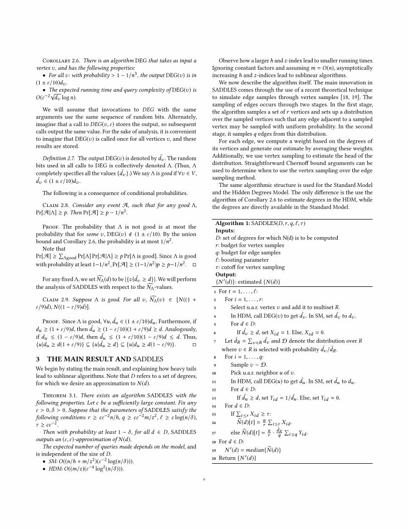
We now describe the algorithm itself. The main innovation inSADDLES comes through the use of a recent theoretical techniqueto simulate edge samples through vertex samples [18, 19]. Thesampling of edges occurs through two stages. In the first stage,the algorithm samples a set of r vertices and sets up a distributionover the sampled vertices such that any edge adjacent to a sampledvertex may be sampled with uniform probability. In the secondstage, it samples q edges from this distribution.

For each edge, we compute a weight based on the degrees ofits vertices and generate our estimate by averaging these weights.Additionally, we use vertex sampling to estimate the head of thedistribution. Straightforward Chernoff bound arguments can beused to determine when to use the vertex sampling over the edgesampling method.

The same algorithmic structure is used for the Standard Modeland the Hidden Degrees Model. The only difference is the use thealgorithm of Corollary 2.6 to estimate degrees in the HDM, whilethe degrees are directly available in the Standard Model.

Algorithm 1: SADDLES(D, r ,q, ℓ,τ )Inputs:D: set of degrees for which N(d) is to be computedr : budget for vertex samplesq: budget for edge samplesℓ: boosting parameterτ : cutoff for vertex samplingOutput:N ′(d): estimated N (d)1 For t = 1, . . . , ℓ:2 For i = 1, . . . , r :3 Select u.a.r. vertex v and add it to multiset R.4 In HDM, call DEG(v) to get dv . In SM, set dv to dv .5 For d ∈ D:6 If dv ≥ d , set Xid = 1. Else, Xid = 0.7 Let dR =

∑v ∈R dv and D denote the distribution over R

where v ∈ R is selected with probability dv/dR .8 For i = 1, . . . ,q:9 Sample v ∼ D.

10 Pick u.a.r. neighbor u of v .11 In HDM, call DEG(u) to get du . In SM, set du to du .12 For d ∈ D:13 If du ≥ d , set Yid = 1/du . Else, set Yid = 0.14 For d ∈ D:15 If

∑i≤r Xid ≥ τ :

16 N (d)[t] = nr

∑i≤r Xid .

17 else N (d)[t] = nr · dRq

∑i≤q Yid .

18 For d ∈ D:19 N ′(d) =medianN (d)20 Return N ′(d)

6

The core theoretical bound: The central technical bound dealswith the properties of each individual estimate N (d)[t].

Theorem 3.2. Suppose r ≥ cε−2n/h, q ≥ cε−2m/z2, τ = cε−2.Then, for alld ∈ D, with probability ≥ 5/6, N (d)[t] ∈ [(1−ε/2)N ((1+ε/2)d), (1 + ε/2)N ((1 − ε/2)d].

The proof of this theorem is the main part of our analysis, whichappears in the next section. Theorem 3.1 can be derived from thistheorem, as we show next.

Proof. (of Theorem 3.1) First, let us prove the error/accuracybound. For a fixed d ∈ D and t ≤ ℓ, Theorem 3.2 asserts thatwe get an accurate estimate with probability ≥ 5/6. Among the ℓindependent invocations, the probability that more than ℓ/3 valuesof N (d)[t] lie outside [(1− ε/2)N ((1+ ε/2)d), (1+ ε/2)N ((1− ε/2)d]is at most exp(−ℓ/100) (by the Chernoff bound of Theorem 2.1). Bythe choice of ℓ ≥ c log(n/δ ), the probability is at most δ/n. Thus,with probability > 1 − δ/n, the median of N (d)[t] gives an (ε, ε)estimate of N (d). By a union bound over all (at most n) d ∈ D, thetotal probability of error over any d is at most δ .

Now for the query complexity. The overall algorithm is the samefor both models, involving multiple invocations of SADDLES. Theonly difference is in DEG, which is trivial when degree queriesare allowed. For the Standard Model, the number of graph queriesmade for a single invocation of SADDLES is simply O(ℓ(r + q))= O(ε−2(n/h +m/z2) log(n/δ )).

For the Hidden Degrees Model, we have to account for theoverhead of Corollary 2.6 for each degree estimated. The numberof queries for a single call to DEG(d) is O(ε−2

√dv logn). The

total overhead of all calls in Step 4 is E[∑v ∈R√dv (ε−2 logn)].

By linearity of expectation, this is O((ε−2 logn)rE[√dv ], where

the expectation is over a uniform random vertex. We can boundrE[

√dv ] ≤ rE[dv ] = O(ε−2n(m/n)/h) = O(ε−2n/h).

The total overhead of all calls in Step 11 requires more care.Note that when DEG(v) is called multiple times for a fixed v , thesubsequent calls require no further queries. (This is because theoutput of the first call can be stored.) We partition the verticesinto two sets S0 = v |dv ≤ z2 and S1 = v |dv > z2. The totalquery cost of queries to S0 is at most O(qz) = O((ε−2 logn)m/z).For the total cost to S1, we directly bound by (ignoring the ε−2 lognfactor)

∑v ∈S1

√dv =

∑v ∈S1 dv/

√dv ≤ z−1

∑v dv = O(m/z). All

in all, the total query complexity isO((ε−4 log2 n)(n/h+m/z)). Sincem ≥ n and z ≤ h, we can simplify to O((ε−4 log2 n)(m/z)).

4 ANALYSIS OF SADDLESWe now prove Theorem 3.2. There are a number of intermediateclaims towards that. We will fix d ∈ D and a choice of t . Abusingnotation, we use N (d) to refer to N (d)[t]. The estimate of Step 16can be analyzed with a direct Chernoff bound.

Claim 4.1. The following holds with probability > 9/10. IfSADDLES(r ,q) outputs an estimate in Step 16 for a given d , thenN (d) ∈ (1 ± ε/10)NΛ(d). If it does not output in Step 16, thenNΛ(d) < (2c/ε2)(n/r ).

Proof. EachXi is an iid Bernoulli random variable, with successprobability precisely NΛ(d)/n. We split into two cases.

Case 1: NΛ(d) ≥ (c/10ε2)(n/r ). By the Chernoff bound ofTheorem 2.1, Pr[|∑i≤r Xi − r NΛ(d)/n | ≥ (ε/10)(r NΛ(d)/n)] ≤2 exp(−(ε2/100)(r NΛ(d)/n) ≤ 1/100.

Case 2: NΛ(d) ≤ (c/10ε2)(n/r ). Note that E[∑i≤r Xi ] ≤ c/10ε2≤ (c/ε2)/2e . By the upper tail bound of Theorem 2.1, Pr[∑i≤r Xi ≥c/ε2] < 1/100.

Thus, with probability at least 99/100, if an estimate is output inStep 16, NΛ(d) > (c/10ε2)(n/r ). By the first case, with probabilityat least 99/100, N (d) is a (1 + ε/10)-estimate for NΛ(d). A unionbound completes the first part.

Furthermore, if NΛ(d) ≥ (2c/ε2)(n/r ), then with probability atleast 99/100, ∑i≤r Xi ≥ (1 − ε/10)r NΛ(d)/n ≥ c/ε2 = τ . A unionbound proves (the contrapositive of) the second part.

We define weights of ordered edges. The weight only depends onthe second member in the pair, but allows for a more convenientanalysis. The weight of ⟨v,u⟩ is the random variable Yi of Step 13.

Definition 4.2. The d-weight of an ordered edge ⟨v,u⟩ for agiven Λ (the randomness of DEG) is defined as follows. We setwtΛ,d (⟨v,u⟩) to be 1/du if du ≥ d , and zero otherwise. For vertexv , wtΛ,d (v) =

∑u ∈Γ(v)wtΛ,d (⟨v,u⟩).

The utility of the weight definition is captured by the followingclaim. The total weight is an approximation of N (d), and thus, wecan analyze how well SADDLES approximates the total weight.

Claim 4.3. If Λ is good,∑v ∈V wtΛ,d (v) ∈ (1 ± ε/9)NΛ(d).

Proof.∑v ∈V

wtΛ,d (v) =∑v ∈V

∑u ∈Γ(v)

1du ≥d/du

=∑

u :du ≥d

∑v ∈Γ(u)

1/du =∑

u :du ≥d

du/du (1)

Since Λ is good, ∀u, du ∈ (1 ± ε/10)du , and du/du ∈ (1 ± ε/9).Applying in (1),

∑v ∈V wtΛ,d (v) ∈ (1 ± ε/9)NΛ(d).

We come to an important lemma, that shows that the weightof the random subset R (chosen in Step 3) is well-concentrated.This is proven using a Chernoff bound, but we need to bound themaximum possible weight to get a good bound on r = |R |.

Lemma 4.4. Fix any good Λ and d . Suppose r ≥ cε−2n/d . Withprobability at least 9/10, ∑v ∈R wtΛ,d (v) ∈ (1 ± ε/8)(r/n)NΛ(d).

Proof. Let wt(R) denote∑v ∈R wtΛ,d (v). By linearity of

expectation, E[wt(R)] = (r/n)· ∑v ∈V wtΛ,d (v) ≥ (r/2n)NΛ(d). Toapply the Chernoff bound, we need to bound the maximum weightof a vertex. For good Λ, the weight wtΛ,d of any ordered pair is atmost 1/(1 − ε/10)d ≤ 2/d . The number of neighbors of v such thatdu ≥ d is at most NΛ(d). Thus, wtΛ,d (v) ≤ 2NΛ(d)/d .

By the Chernoff bound of Theorem 2.1 and setting r ≥ cε−2n/d ,

Pr [|wt(R) − E[wt(R)]| > (ε/20)E[wt(R)]]

< 2 exp(−ε

2 · (cε−2n/d) · (NΛ(d)/2n)3 · 202 · 2NΛ(d)/d

)≤ 1/10

7

With probability at least 9/10, wt(R) ∈ (1 ± ε/20)E[wt(R)]. Bythe arguments given above, E[wt(R)] ∈ (1 ± ε/9)(r/n)NΛ(d). Wecombine to complete the proof.

Now, we determine the number of edge samples required toestimate the weight wtΛ,d (R).

Lemma 4.5. Let N (d) be as defined in Step 17 of SADDLES.Assume Λ is good, r ≥ cε−2n/d , and q ≥ cε−2m/(dNΛ(d)). Then,with probability > 7/8, N (d) ∈ (1 ± ε/4)NΛ(d).

Proof. We define the random set R selected in Step 3 to besound if the following hold. (1) wt(R) = ∑

v ∈R wtΛ,d (v) ∈ (1 ±ε/8)(r/n)NΛ(d) and (2)

∑v ∈R dv ≤ 100r (2m/n). By Lemma 4.4, the

first holds with probability > 9/10. Observe that E[∑v ∈R dv ] =r (2m/n), since 2m/n is the average degree. By the Markov bound,the second holds with probability > 99/100. By the union bound, Ris sound with probability at least 1 − (1/10 + 1/100) > 8/9.

Fix a sound R. Recall Yi from Step 13. The expectation of Yi |R is∑v ∈R Pr[v is selected]·∑u ∈Γ(v) Pr[u is selected]wtΛ,d (⟨v,u⟩). We

plug in the probability values, and observe that for good Λ, for allv , dv/dv ∈ (1 ± ε/10).

E[Yi |R] =∑v ∈R

(dv/dR )∑

u ∈Γ(v)(1/dv )wtΛ,d (⟨v,u⟩)

= (1/dR )∑v ∈R

(dv/dv )∑

u ∈Γ(v)wtΛ,d (⟨v,u⟩)

∈ (1 ± ε/10)(1/dR )∑v ∈R

∑u ∈Γ(v)

wtΛ,d (⟨v,u⟩)

∈ (1 ± ε/10)(wt(R)/dR ) (2)

Note that N (d) = (n/r )(dR/q)∑i≤q Yi and

(n/r )(dR/q)E[∑i≤q Yi |R] ∈ (1 ± ε/10)(n/r )wt(R). Since R is

sound, the latter is in (1 ± ε/4)NΛ(d). Also, note that

E[Yi |R] = E[Y1 |R] ≥qwt(R)2dR

≥ (r/n)NΛ(d)4(100r (2m/n) =

NΛ(d)800m (3)

By linearity of expectation, E[∑i≤q Yi |R] = qE[Y1 |R]. Observe thatYi ≤ 1/d . We can apply the Chernoff bound of Theorem 2.1 to theiid random variables (Yi |R).

Pr[|∑iYi − E[

∑iYi ]| > (ε/100)E[

∑iYi ]|R]

≤ 2 exp(− ε2

3 · 1002· d · qE[Y1 |R]

)(4)

We use (3) to bound the (positive) term in the exponent is at least

ε2

3 · 1002· cε

−2m

NΛ(d)· NΛ(d)800m ≥ 10.

Thus, if R is sound, the following bound holds with probability atleast 0.99. We also apply (2).

NΛ(d) = (n/r )(dR/q)q∑i=1

Yi

∈ (1 ± ε/100)(n/r )(dR/q)qE[Yi |R]∈ (1 ± ε/100)(1 ± ε/10)(n/r )wt(R) ∈ (1 ± ε/4)N (d)

The probability that R is sound is at least 8/9. A union boundcompletes the proof.

The bounds on r and q in Lemma 4.5 depend on the degree d .We now bring in the h and z-indices to derive bounds that hold forall d . We also remove the conditioning over a good Λ.

Proof. (of Theorem 3.2) We will first assume that Λ is good. ByClaim 2.9, NΛ(d) ∈ [N ((1 + ε/9)d,N ((1 − ε/9)d)].

Suppose NΛ(d) = 0, so there are no vertices with dv ≥ d . By thebound above, N ((1 + ε/9)d) = 0, implying that N ((1 + ε/2)d) = 0.Furthermore N (d) = 0, since the random variables Xi and Yi inSADDLES can never be non-zero. Thus, N (d) = N ((1 + ε/2)d),completing the proof.

We now assume that NΛ(d) > 0. We split into two cases,depending on whether Step 16 outputs or not. By Claim 4.1, withprobability > 9/10, if Step 16 outputs, then N (d) ∈ (1 ± ε/9)NΛ(d).By combining these bounds, the desired bound on N (d) holds withprobability > 9/10, conditioned on a good Λ.

Henceforth, we focus on the case that Step 16 does not output.By Claim 4.1, NΛ(d) < 2cε−2(n/r ). By the choice of r and Claim 2.9,NΛ((1 + ε/9)d) < h. By the characterization of h of Lemma 2.2,z2 ≤ max(NΛ((1+ε/9)d), (1+ε/9)d) = (1+ε/9)d . This implies thatr ≥ cε−2n/d . By the definition of z, z2 ≤ N (min(dmax , (1+ε/9)d)) ·min(dmax , (1+ε/9)d). By the Claim 2.9 bound in the first paragraph,NΛ(d) ≥ N ((1+ε/9)d). Since NΛ(d) > 0, NΛ(d) ≥ NΛ(dmax ). Thus,z2 ≤ NΛ(d) · (1 + ε/9)d . and hence, m ≤ cε−2m/(dNΛ(d)). Theparameters satisfy the conditions in Lemma 4.5. With probability> 7/8, N (d) ∈ (1 ± ε/4)NΛ(d), and by Claim 2.9, N (d) has thedesired accuracy.

All in all, assuming Λ is good, with probability at least 7/8, N (d)has the desired accuracy. The conditioning on a good Λ is removedby Claim 2.8 to complete the proof.

5 EXPERIMENTAL RESULTSWe implemented our algorithm in C++ and performed ourexperiments on a MacBook Pro laptop with 2.7 GHz Intel Corei5 with 8 GB RAM. We performed our experiments on a collectionof graphs from SNAP [29], including social networks, web networks,and infrastructure networks. The graphs typically have millionsof edges, with the largest having more than 100M edges. Basicproperties of these graphs are presented in Table 1. We ignoredirection and treat all edges as undirected edges.

5.1 Implementation DetailsFor the HDM, we explicitly describe the procedure DEG(v), whichestimates the degree of a given vertex (v). In the algorithm DEG,

Algorithm 2: DEG(v)1 (Initialize S = ∅.) Repeatedly add u.a.r. vertex to S , until the

number of pair-wise collisions is at least k = 25.2 Output

( |S |2)/k as estimate dv .

a “pair-wise collision" refers to a pair of neighbor samples thatyield the same vertex. The expected number of pair-wise collisionsis

( |S |2)/dv . We simply reverse engineer that inequality to get the

8

estimate dv . Ron and Tsur essentially prove that this estimate haslow variance [41].

Setting the parameter values. The boosting parameter ℓ issimply set to 1. (In some sense, we only introduced the medianboosting for the theoretical union bound. In practice, convergenceis much more rapid that predicted by the Chernoff bound.)

The threshold τ is set to 100. The parameters r and q are chosento be typically around 0.005n. These are not “sublinear" per se, butare an order of magnitude smaller than the queries made in existinggraph sampling results (more discussion in next section).

We set D = ⌊1.1i ⌋, since that gives a sufficiently fine-grainedapproximation at all scales of the degree distribution.

Code for all experiments is available here1.

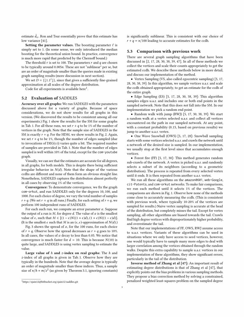
5.2 Evaluation of SADDLESAccuracy over all graphs:We run SADDLESwith the parametersdiscussed above for a variety of graphs. Because of spaceconsiderations, we do not show results for all graphs in thisversion. (We discovered the results to be consistent among all ourexperiments.) Fig. 1 show the results for the SM for some graphsin Tab. 1. For all these runs, we set r + q to be 1% of the number ofvertices in the graph. Note that the sample size of SADDLES in theSM is exactly r + q. For the HDM, we show results in Fig. 2. Again,we set r + q to be 1%, though the number of edges sampled (dueto invocations of DEG(v)) varies quite a bit. The required numberof samples are provided in Tab. 1. Note that the number of edgessampled is well within 10% of the total, except for the com-youtubegraph.

Visually, we can see that the estimates are accurate for all degrees,in all graphs, for both models. This is despite there being sufficientirregular behavior in N (d). Note that the shape of the variousccdhs are different and none of them form an obvious straight line.Nonetheless, SADDLES captures the distribution almost perfectlyin all cases by observing 1% of the vertices.

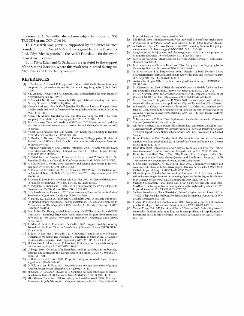
Convergence: To demonstrate convergence, we fix the graphcom-orkut, and run SADDLES only for the degrees 10, 100, and1000. For each choice of degree, we vary the total number of samplesr +q. (We set r = q in all runs.) Finally, for each setting of r +q, weperform 100 independent runs of SADDLES.

For each such run, we compute an error parameter α . Supposethe output of a run isM , for degree d . The value of α is the smallestvalue of ϵ , such that M ∈ [(1 − ϵ)N ((1 + ϵ)d), (1 + ϵ)N ((1 − ϵ)d)].(It is the smallest ϵ such thatM is an (ϵ, ϵ)-approximation of N (d).)

Fig. 3 shows the spread of α , for the 100 runs, for each choiceof r + q. Observe how the spread decreases as r + q goes to 10%.In all cases, the values of α decay to less than 0.05. We notice thatconvergence is much faster for d = 10. This is because N (10) isquite large, and SADDLES is using vertex sampling to estimate thevalue.

Large value of h and z-index on real graphs: The h andz-index of all graphs is given in Tab. 1. Observe how they aretypically in the hundreds. Note that the average degree is typicallyan order of magnitude smaller than these indices. Thus, a samplesize of n/h +m/z2 (as given by Theorem 3.1, ignoring constants)

1https://sjain12@bitbucket.org/sjain12/saddles.git

is significantly sublinear. This is consistent with our choice ofr + q = n/100 leading to accurate estimates for the ccdh.

5.3 Comparison with previous workThere are several graph sampling algorithms that have beendiscussed in [2, 17, 28, 30, 38, 39, 47]. In all of these methods wecollect the vertices and scale their counts appropriately to get theestimated ccdh. We describe these methods below in more detail,and discuss our implementation of the method.

• Vertex Sampling (VS, also called egocentric sampling) [5, 17,28, 30, 38, 39]: In this algorithm, we sample vertices u.a.r. and scalethe ccdh obtained appropriately, to get an estimate for the ccdh ofthe entire graph.

• Edge Sampling (ES) [5, 17, 28, 30, 38, 39]: This algorithmsamples edges u.a.r. and includes one or both end points in thesampled network. Note that this does not fall into the SM. In ourimplementation we pick a random end point.

• Random walk with jump (RWJ) [5, 17, 30, 38, 39]: We starta random walk at a vertex selected u.a.r. and collect all verticesencountered on the path in our sampled network. At any point,with a constant probability (0.15, based on previous results) wejump to another u.a.r. vertex.

• One Wave Snowball (OWS) [5, 17, 28]: Snowball samplingstarts with some vertices selected u.a.r. and crawls the network untila network of the desired size is sampled. In our implementation,we usually stop at the first level since that accumulates enoughvertices.

• Forest fire (FF) [5, 17, 30]: This method generates randomsub-crawls of the network. A vertex is picked u.a.r. and randomlyselects a subset of its neighbors (according to a geometricdistribution). The process is repeated from every selected vertexuntil it ends. It is then repeated from another u.a.r. vertex.

We run all these algorithms on the amazon0601, web-Google,cit-Patents, and com-orkut networks. To make fair comparisons,we run each method until it selects 1% of the vertices. Thecomparisons are shown in Fig. 1. Observe how none of the methodscome close to accurately measuring the ccdh. (This is consistentwith previous work, where typically 10-20% of the vertices aresampled for results.) Naive vertex sampling is accurate at the headof the distribution, but completely misses the tail. Except for vertexsampling, all other algorithms are biased towards the tail. Crawlsfind high degree vertices with disproportionately higher probability,and overestimate the tail.

Note that our implementations of FF, OWS, RWJ assume accessto u.a.r. vertices. Variants of these algorithms can be used insituations where we only have access to seed vertices, however,one would typically have to sample many more edges to deal withlarger correlation among the vertices obtained through the randomwalks. Despite this extra capability to sample u.a.r. vertices in ourimplementation of these algorithms, they show significant errors,particularly in the tail of the distribution.

Inverse method of Zhang et al [47]: An important result ofestimating degree distributions is that of Zhang et al [47], thatexplicitly points out the bias problems in various sampling methods.They propose a bias correction method by solving a constrained,penalized weighted least-squares problem on the sampled degree

9

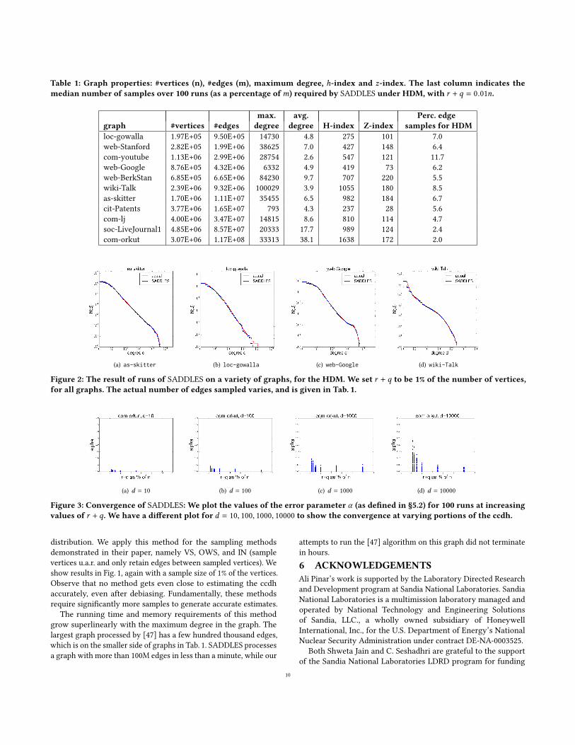
Table 1: Graph properties: #vertices (n), #edges (m), maximum degree, h-index and z-index. The last column indicates themedian number of samples over 100 runs (as a percentage ofm) required by SADDLES under HDM, with r + q = 0.01n.

max. avg. Perc. edgegraph #vertices #edges degree degree H-index Z-index samples for HDMloc-gowalla 1.97E+05 9.50E+05 14730 4.8 275 101 7.0web-Stanford 2.82E+05 1.99E+06 38625 7.0 427 148 6.4com-youtube 1.13E+06 2.99E+06 28754 2.6 547 121 11.7web-Google 8.76E+05 4.32E+06 6332 4.9 419 73 6.2web-BerkStan 6.85E+05 6.65E+06 84230 9.7 707 220 5.5wiki-Talk 2.39E+06 9.32E+06 100029 3.9 1055 180 8.5as-skitter 1.70E+06 1.11E+07 35455 6.5 982 184 6.7cit-Patents 3.77E+06 1.65E+07 793 4.3 237 28 5.6com-lj 4.00E+06 3.47E+07 14815 8.6 810 114 4.7soc-LiveJournal1 4.85E+06 8.57E+07 20333 17.7 989 124 2.4com-orkut 3.07E+06 1.17E+08 33313 38.1 1638 172 2.0

(a) as-skitter (b) loc-gowalla (c) web-Google (d) wiki-Talk

Figure 2: The result of runs of SADDLES on a variety of graphs, for the HDM. We set r + q to be 1% of the number of vertices,for all graphs. The actual number of edges sampled varies, and is given in Tab. 1.

(a) d = 10 (b) d = 100 (c) d = 1000 (d) d = 10000

Figure 3: Convergence of SADDLES: We plot the values of the error parameter α (as defined in §5.2) for 100 runs at increasingvalues of r + q. We have a different plot for d = 10, 100, 1000, 10000 to show the convergence at varying portions of the ccdh.

distribution. We apply this method for the sampling methodsdemonstrated in their paper, namely VS, OWS, and IN (samplevertices u.a.r. and only retain edges between sampled vertices). Weshow results in Fig. 1, again with a sample size of 1% of the vertices.Observe that no method gets even close to estimating the ccdhaccurately, even after debiasing. Fundamentally, these methodsrequire significantly more samples to generate accurate estimates.

The running time and memory requirements of this methodgrow superlinearly with the maximum degree in the graph. Thelargest graph processed by [47] has a few hundred thousand edges,which is on the smaller side of graphs in Tab. 1. SADDLES processesa graph with more than 100M edges in less than a minute, while our

attempts to run the [47] algorithm on this graph did not terminatein hours.6 ACKNOWLEDGEMENTSAli Pinar’s work is supported by the Laboratory Directed Researchand Development program at Sandia National Laboratories. SandiaNational Laboratories is a multimission laboratory managed andoperated by National Technology and Engineering Solutionsof Sandia, LLC., a wholly owned subsidiary of HoneywellInternational, Inc., for the U.S. Department of Energy’s NationalNuclear Security Administration under contract DE-NA-0003525.

Both Shweta Jain and C. Seshadhri are grateful to the supportof the Sandia National Laboratories LDRD program for funding

10

this research. C. Seshadhri also acknowledges the support of NSFTRIPODS grant, CCF-1740850.

This research was partially supported by the Israel ScienceFoundation grant No. 671/13 and by a grant from the Blavatnikfund. Talya Eden is grateful to the Azrieli Foundation for the awardof an Azrieli Fellowship.

Both Talya Eden and C. Seshadhri are grateful to the supportof the Simons Institute, where this work was initiated during theAlgorithms and Uncertainty Semester.

REFERENCES[1] D. Achlioptas, A. Clauset, D. Kempe, and C. Moore. 2009. On the bias of traceroute

sampling: Or, power-law degree distributions in regular graphs. J. ACM 56, 4(2009).

[2] N.K. Ahmed, J. Neville, and R. Kompella. 2010. Reconsidering the Foundations ofNetwork Sampling. In WIN 10.

[3] N. Ahmed, J. Neville, and R. Kompella. 2012. Space-Efficient Sampling from SocialActivity Streams. In SIGKDD BigMine. 1–8.

[4] Nesreen K Ahmed, Nick Duffield, Jennifer Neville, and Ramana Kompella. 2014.Graph sample and hold: A framework for big-graph analytics. In SIGKDD. ACM,ACM, 1446–1455.

[5] Nesreen K Ahmed, Jennifer Neville, and Ramana Kompella. 2014. Networksampling: From static to streaming graphs. TKDD 8, 2 (2014), 7.

[6] Sinan G. Aksoy, Tamara G. Kolda, and Ali Pinar. 2017. Measuring and modelingbipartite graphs with community structure. Journal of Complex Networks (2017).to appear.

[7] Albert-László Barabási and Réka Albert. 1999. Emergence of Scaling in RandomNetworks. Science 286 (Oct. 1999), 509–512.

[8] A. Broder, R. Kumar, F. Maghoul, P. Raghavan, S. Rajagopalan, R. Stata, A.Tomkins, and J. Wiener. 2000. Graph structure in the web. Computer Networks33 (2000), 309–320.

[9] Deepayan Chakrabarti and Christos Faloutsos. 2006. Graph Mining: Laws,Generators, and Algorithms. Comput. Surveys 38, 1 (2006). https://doi.org/10.1145/1132952.1132954

[10] F. Chierichetti, A. Dasgupta, R. Kumar, S. Lattanzi, and T. Sarlos. 2016. OnSampling Nodes in a Network. In Conference on the World Wide Web (WWW).

[11] A. Clauset and C. Moore. 2005. Accuracy and scaling phenomena in internetmapping. Phys. Rev. Lett. 94 (2005), 018701.

[12] A. Clauset, C. R. Shalizi, and M. E. J. Newman. 2009. Power-Law Distributionsin Empirical Data. SIAM Rev. 51, 4 (2009), 661–703. https://doi.org/10.1137/070710111

[13] R. Cohen, K. Erez, D. ben Avraham, and S. Havlin. 2000. Resilience of the Internetto Random Breakdowns. Phys. Rev. Lett. 85, 4626âĂŞ8 (2000).

[14] A. Dasgupta, R. Kumar, and T. Sarlos. 2014. On estimating the average degree. InConference on the World Wide Web (WWW). 795–806.

[15] D. Dubhashi and A. Panconesi. 2012. Concentration of Measure for the Analysis ofRandomised Algorithms. Cambridge University Press.

[16] N. Durak, T.G. Kolda, A. Pinar, and C. Seshadhri. 2013. A scalable null modelfor directed graphs matching all degree distributions: In, out, and reciprocal. InNetwork Science Workshop (NSW), 2013 IEEE 2nd. 23–30. https://doi.org/10.1109/NSW.2013.6609190

[17] Peter Ebbes, Zan Huang, Arvind Rangaswamy, Hari P Thadakamalla, and ORGBUnit. 2008. Sampling large-scale social networks: Insights from simulatednetworks. In 18th Annual Workshop on Information Technologies and Systems,Paris, France.

[18] T. Eden, A. Levi, D. Ron, and C. Seshadhri. 2015. Approximately CountingTriangles in Sublinear Time. In Foundations of Computer Science (FOCS), GRS11(Ed.). 614–633.

[19] T. Eden, D. Ron, and C. Seshadhri. 2017. Sublinear Time Estimation of DegreeDistribution Moments: The Degeneracy Connection. In International Colloquiumon Automata, Languages, and Programming (ICALP), GRS11 (Ed.). 614–633.

[20] M. Faloutsos, P. Faloutsos, and C. Faloutsos. 1999. On power-law relationships ofthe internet topology. In SIGCOMM. 251–262.

[21] U. Feige. 2006. On sums of independent random variables with unboundedvariance and estimating the average degree in a graph. SIAM J. Comput. 35, 4(2006), 964–984.

[22] O. Goldreich and D. Ron. 2002. Property Testing in Bounded Degree Graphs.Algorithmica (2002), 302–343.

[23] O. Goldreich and D. Ron. 2008. Approximating average parameters of graphs.Random Structures and Algorithms 32, 4 (2008), 473–493.

[24] M. Gonen, D. Ron, and Y. Shavitt. 2011. Counting stars and other small subgraphsin sublinear-time. SIAM Journal on Discrete Math 25, 3 (2011), 1365–1411.

[25] Mira Gonen, Dana Ron, Udi Weinsberg, and Avishai Wool. 2008. Finding adense-core in Jellyfish graphs. Computer Networks 52, 15 (2008), 2831–2841.

https://doi.org/10.1016/j.comnet.2008.06.005[26] J. E. Hirsch. 2005. An index to quantify an individual’s scientific research output.

Proceedings of the National Academy of Sciences 102, 46 (2005), 16569âĂŞ16572.[27] A. Lakhina, J. Byers, M. Crovella, and P. Xie. 2003. Sampling biases in IP topology

measurements. In Proceedings of INFOCOMM, Vol. 1. 332–341.[28] Sang Hoon Lee, Pan-Jun Kim, and Hawoong Jeong. 2006. Statistical properties

of sampled networks. Physical Review E 73, 1 (2006), 016102.[29] Jure Leskovec. 2015. SNAP Stanford Network Analysis Project. http://snap.

standord.edu. (2015).[30] Jure Leskovec and Christos Faloutsos. 2006. Sampling from large graphs. In

Knowledge Data and Discovery (KDD). ACM, 631–636.[31] A. S. Maiya and T. Y. Berger-Wolf. 2011. Benefits of Bias: Towards Better

Characterization of Network Sampling, In Knowledge Data and Discovery (KDD).ArXiv e-prints, 105–113. arXiv:1109.3911

[32] Andrew McGregor. 2014. Graph stream algorithms: A survey. SIGMOD 43, 1(2014), 9–20.

[33] M. Mitzenmacher. 2003. A Brief History of Generative Models for Power Lawand Lognormal Distributions. Internet Mathematics 1, 2 (2003), 226–251.

[34] M. E. J. Newman. 2003. The Structure and Function of Complex Networks. SIAMRev. 45, 2 (2003), 167–256. https://doi.org/10.1137/S003614450342480

[35] M. E. J. Newman, S. Strogatz, and D. Watts. 2001. Random graphs with arbitrarydegree distributions and their applications. Physical Review E 64 (2001), 026118.

[36] D. Pennock, G. Flake, S. Lawrence, E. Glover, and C. L. Giles. 2002. Winners don’ttake all: Characterizing the competition for links on the web. Proceedings of theNational Academy of Sciences 99, 8 (2002), 5207–5211. https://doi.org/10.1073/pnas.032085699

[37] T. Petermann and P. Rios. 2004. Exploration of scale-free networks. EuropeanPhysical Journal B 38 (2004), 201–204.

[38] Ali Pinar, Sucheta Soundarajan, Tina Eliassi-Rad, and Brian Gallagher. 2015.MaxOutProbe: An Algorithm for Increasing the Size of Partially Observed Networks.Technical Report. Sandia National Laboratories (SNL-CA), Livermore, CA (UnitedStates).

[39] Bruno Ribeiro and Don Towsley. 2012. On the estimation accuracy of degreedistributions from graph sampling. In Annual Conference on Decision and Control(CDC). IEEE, 5240–5247.

[40] Dana Ron. 2010. Algorithmic and Analysis Techniques in Property Testing.Foundations and Trends in Theoretical Computer Science 5, 2 (2010), 73–205.

[41] Dana Ron and Gilad Tsur. 2016. The Power of an Example: Hidden SetSize Approximation Using Group Queries and Conditional Sampling. ACMTransactions on Computation Theory 8, 4 (2016), 15:1–15:19.

[42] C. Seshadhri, Tamara G. Kolda, and Ali Pinar. 2012. Community structure andscale-free collections of Erdös-Rényi graphs. Physical Review E 85, 5 (May 2012),056109. https://doi.org/10.1103/PhysRevE.85.056109

[43] Olivia Simpson, C Seshadhri, and Andrew McGregor. 2015. Catching the head,tail, and everything in between: a streaming algorithm for the degree distribution.In International Conference on Data Mining (ICDM). IEEE, 979–984.

[44] Sucheta Soundarajan, Tina Eliassi-Rad, Brian Gallagher, and Ali Pinar. 2016.MaxReach: Reducing network incompleteness through node probes. 152–157.https://doi.org/10.1109/ASONAM.2016.7752227

[45] Sucheta Soundarajan, Tina Eliassi-Rad, Brian Gallagher, and Ali Pinar. 2017. ϵ- WGX: Adaptive Edge Probing for Enhancing Incomplete Networks. In WebScience Conference. 161–170.

[46] Michael PH Stumpf and Carsten Wiuf. 2005. Sampling properties of randomgraphs: the degree distribution. Physical Review E 72, 3 (2005), 036118.

[47] Yaonan Zhang, Eric D Kolaczyk, and Bruce D Spencer. 2015. Estimating networkdegree distributions under sampling: An inverse problem, with applications tomonitoring social media networks. The Annals of Applied Statistics 9, 1 (2015),166–199.

11