talent, geography, and offshore r&d
TRANSCRIPT

Talent, Geography, and Offshore R&D∗
Jingting Fan†
This draft: October 2019
Abstract
I model and quantify the impact of a new dimension of global integration: off-
shore R&D. In the model, firms match with heterogeneous researchers to develop new
product blueprints, and then engage in offshore production and exporting. Cross-
country differences in the distributions of firm efficiency and researcher talent gener-
ate a “talent-acquisition” motive for offshore R&D, while trade costs and the frictions
impeding separation of R&D from production lead to a “market-access” motive. I
find evidence for the premise of both motives using a new firm-country level data of
R&D and production. Counterfactuals using the calibrated model show that interna-
tional differences in endowment distributions and the market access motive collec-
tively account for most of the observed offshore R&D. Increasing offshore production
to emerging countries may or may not lead to a large increase in offshore R&D, de-
pending on the fundamental force driving the offshore production increase. In terms
of welfare, incorporating offshore R&D amplifies the gains from global integration by
a factor of 1.2, and has important implications for the welfare gains from traditional
forms of global integration, namely trade and offshore production
Keywords: Gains from openness, multinational firms, offshore R&D, global value
chain, the smile curve
JEL Classification: F21 F23 F40 O32
∗I am deeply grateful to Nuno Limao for his encouragement and guidance throughout my graduatestudy, and to my committee Sebnem Kalemli-Özcan and John Shea for their invaluable feedback, whichgreatly improved the paper. I thank Ariel Burstein, Kamran Bilir, Jonathan Eaton, Gordon Hanson, Wolf-gang Keller, Eunhee Lee, Wenlan Luo, James Markusen, Luca Opromolla, Natalia Ramondo, AndresRodriguez-Clare, Marisol Rodriguez-Chatruc, Felipe Saffie, Lixin Tang, Jim Tybout, Daniel Wilson, StephenYeaple, and seminar participants at numerous institutions and conferences for helpful comments. All errorsare mine.†Department of Economics, Penn State University. Email address: [email protected]
1

1 Introduction
A common narrative of the recent wave of globalization is that reductions in trade barri-ers and communication costs enabled firms from developed countries to offshore the ‘lowvalue-added’ production tasks overseas and specialize at home in ‘high value-added’,skill-intensive tasks such conception, R&D, and marketing. In line with this view, theliterature on multinational production1 and global value chain (GVC) has largely focusedon the causes and consequences of the allocation of production (or different stages of pro-duction) across countries. This view captures only partially the complex strategies usedby modern firms in organizing commerce around the globe, however. Increasingly, firmsengage not only in production but also in R&D activities in their overseas affiliates.2 Asshown in Figure 1, in many host countries, the R&D carried out by foreign firms amountsto a substantial and growing fraction of the total R&D.
The significance of offshore R&D in the data raises a number of questions. From apositive perspective, what are the factors behind firms decision to allocate R&D abroad,and how does the option of doing so affect each country’s specialization in the innova-tion versus production stages of the GVC? From a normative perspective, what are theimplications of offshore R&D for the aggregate efficiency and distributional outcomes,and how do the answer depend on and interact with trade and offshore production? Inthis paper, I attempt to answer these questions quantitatively by combining micro data ofR&D and production within MNCs with a multi-country general equilibrium model.
My analysis proceeds in two steps. In the first step, I document facts that inform thedriving forces of firms’ organization of activities around the world. At the core of thisanalysis is a newly assembled data set of R&D and production at parent-host countrylevel.3 The production data and the ownership information that links firms to their par-ents are from the Orbis database, which has been used in research on MNCs (see e.g.,Fons-Rosen et al., 2013 and Cravino and Levchenko, 2017). I link firms in this data setto the PATSTAT database, which contains the bibliographic information of patents frommore than 90 patent offices. The location of inventors, collected at the patent applica-tion stage by most patent offices, identifies where the invention underlying each patent
1Throughout this paper, I use the term ‘multinational production’ to refer to cases in which a product isproduced in a location different from where it is developed, as in recent studies (Garetto, 2013; Ramondo,2014; Ramondo and Rodríguez-Clare, 2013; Irarrazabal et al., 2013; Arkolakis et al., 2018; and Tintelnot,2016). This term is closely related to ‘offshore production’ in the offshoring literature. I use these two termsinterchangeably, but emphasize that my theory and measurement focus on offshoring within a firm.
2DuPont offers a good example. Headquartered in Delaware, U.S., it has major R&D centers located inthe U.S., Brazil, China, Switzerland, Korea, Germany, and Japan. Moreover, it has production facilities in19 countries, from which it serves around 90 countries.
3Throughout this paper, a ‘parent’ firm refers to the collection of all firms owned by the same entity. Aparent-host country combination refers to the affiliate of the parent firm in the host country.
2

Figure 1: The Level and Growth of Offshore R&D, 1985-2012
Notes: The measure for offshore R&D in country i is Total private R&D expenditures in country i by foreign firmsTotal private R&D expenditures in country i . Uncolored bars indicate the value
of this variable in 2012; colored bars indicate the value at the beginning of the sample, which differs by country and dates back to asearly as 1985. Data source: OECD.
is conducted. Aggregating across all patents granted to a parent firm, I obtain a measurefor R&D at the parent-host country level. This measure is robust to how an MNC assignpatents to its affiliates within the firm.
Three facts emerge from the data set. First, within a parent, R&D and production tendto co-locate. This fact holds both when we compare different affiliates, or using the over-time variations within an affiliate. Second, both the R&D and production of overseas af-filiates decrease with various measures of distance to headquarters, but in different ways.Third, the R&D intensity of an affiliate, measured as the ratio of R&D to sales, is higher inhost country better human capital and—within an affiliate—increases as the host countryexperiences improvements in human capital quality. Together, these facts highlight thenecessary ingredients of the structural model: 1) the efficiency losses when separatingproduction from R&D, 2) significant but potentially heterogeneous headquarter effectsfor affiliate R&D and production, and 3) the role of host country talent for R&D.
In the second step of analysis, I develop a unified framework of firms’ global R&D andproduction decisions incorporating these ingredients. In the model, firms differ along twodimensions: innovation efficiency, which governs how effective a firm is in convertingresearcher input into new product blueprints, and production efficiency, which governsa firm’s productivity in converting production labor into output. Researchers differ intheir talent. Firms can enter foreign countries (hosts) to perform offshore R&D. In eachhost, the firm matches with local researchers to develop new varieties. I model R&D as anassignment problem between firms and researchers, in which researcher talent and firmefficiency are complements (Sampson, 2014; Grossman et al., 2017). This setup deviates
3

from the efficiency units assumption, and implies that quality and quantity of researchersare not perfect substitutes, an important feature of R&D in reality.4
I embed this offshore R&D decision into a multi-country general equilibrium modelof global production and trade (Arkolakis et al., 2018). Specifically, after a product isdeveloped by an R&D center, whether onshore or offshore, the firm first chooses whichcountries to sell it to, and then decides where to produce it. An American company canthus develop a new product in the U.K., produce it in China, and export from there toIndia. The headquarter services (the rent repatriated to parent firms for their knowhow),R&D, production, and marketing constitutes four stages of a GVC. The flexibility for firmsto conduct these stages in different countries captures the complex strategies employedby modern multinationals.
The model allows for two motives for offshore R&D commonly cited by firms: ‘market-access’ and ‘talent-acquisition’.5 The former is straightforward: to save on production andtrade costs, firms want to produce near their markets and in countries with high manu-facturing productivity and low wages. Because separating innovation from production iscostly, firms have incentives to offshore their R&D to large markets and countries with ahigh manufacturing efficiency. The latter motive depends on both firm and host countrycharacteristics. First, it reflects the host country’s relative abundance of talented inventors,which depends on the abundance of talented inventors—an input supply effect, and theabundance of efficient firms competing for talent—an input demand effect. Second, be-cause of the complementarity in innovation, host relative talent abundance interacts withfirm efficiency to reinforce the talent-acquisition motive for high-efficiency firms.
I calibrate the model to data from 25 countries and a composite of 22 other countries. Iparameterize each country’s distribution of firm efficiency using the World ManagementSurvey developed by Bloom et al. (2012), and its talent distribution using the interna-tional cognitive test score database developed by Hanushek and Woessmann (2012). Idetermine other parameters by matching various statistics of the firm size distribution inthe U.S. and the intensities of bilateral international activities, including trade, offshoreproduction, and offshore R&D. The model matches several non-targeted patterns in thedata reasonably well.
I use the calibrated model for counterfactual experiments to uncover two sets of quan-titative results. The first focuses on the empirical relevance of the two motives in deter-mining offshore R&D. I eliminate the incentives of offshore R&D arising from these dis-
4The output distribution of researchers is highly skewed. Akcigit et al. (2016) shows that the averagetop 1% inventor has 1019 lifetime citations, while the median inventor has only 11.
5According to firm-level surveys (see, for example, Thursby and Thursby, 2006), the quality of researchpersonnel and host country market potential are the two most important factors firms consider, whenchoosing where to build their offshore R&D centers.
4

tribution differences by first giving each individual country the management distributionof U.S. (the highest in the world), and then the talent distribution of Brazil (the lowestin the world). The former reduces the average level of offshore R&D by around threequarters, whereas the latter reduces this average by around one third. So differences inthe distributions of talent and management efficiency are an important driving force foroffshore R&D. I also examine how a country’s access to foreign markets through export-ing, and to foreign producers through offshore production, affect its attractiveness as adestination for R&D. While both consumer and producer access increase the return toinnovation in partial equilibrium, I find that they have opposite general equilibrium ef-fects: consumer access reduces inward offshore R&D, while producer access increases it.Therefore, increasing access to foreign markets through reducing exporting costs wouldnot necessarily help a country in attracting R&D-intensive FDI. Country specialization ininnovation or production is the key to understanding this result. When a country losesaccess to foreign consumers through exporting, its competitiveness in production weak-ens, which lowers wages and makes it more attractive as a host for offshore R&D centers.As a result, it specializes more in innovation, and firms do R&D there and offshore theirproduction to other countries. Such specialization is not possible without offshore pro-duction, so when both consumer and producer access are shut down, the average offshoreR&D across countries decreases to less than half of the benchmark level. Together, thesetwo sets of experiments suggest that the talent-acquisition and market-access motives inthe model are strong enough to account for the observed level of offshore R&D.
Related to the market access motive, there is an increasing concern among the devel-oped world that, with the growth of the Chinese economy (in both size and productivity)and reductions in the cost of offshoring, more and more production will be offshoredto China. Given the co-location of R&D and production, increasingly high value-addedR&D will be offshored, too. While a significant literature has examined the consequencesof China’ rise in production and export on other countries,6 how the rise of manufactur-ing productivity in China will affect the developed country through offshore of R&D isnot yet examined. Through counterfactual experiments, I find that increasing offshoreproduction as a result of improving manufacturing productivity in China will increasesoffshore R&D into China only modestly, due to the general equilibrium effect discussedabove. However, the same increase in offshore production resulting from a decrease inthe cost of offshore production in China encourages offshore R&D significantly—the gen-eral equilibrium effect, while still present, is much weaker because foreign production ac-counts for a small fraction of the Chinese economy. These results highlight the importance
6See e.g., Autor et al. (2013) and the reference thereto for empirical work; See e.g., Levchenko and Zhang(2013); Galle et al. (2017); Caliendo et al. (2019) for model-based simulations.
5

of understanding the nature of the shock that leads to increasing offshore production toemerging countries.
The second set of counterfactual experiments focus on the normative implications ofoffshore R&D. I obtain two results. First, analytically (under a special case) and quan-titatively, I show that the option of conducting R&D abroad generates significant wel-fare gains. The average welfare gains from offshore R&D, defined analogously to thegains from trade, are around 2.5% of real income. Compared to a restricted version of themodel with only trade and offshore production, the welfare gains from openness in thefull model with offshore R&D are larger by a factor of 1.2. This amplification is substan-tially larger for emerging countries than for developed countries, mainly because a largershare of R&D in emerging countries is carried out by foreign affiliates. Overlooking thischannel therefore will not only result in underestimating the gains from globalization, butalso bias the assessment of the relative size of the welfare gains across countries.
The second result is, due to the interaction between innovation and production in aGVC, incorporating offshore R&D is important for understanding the welfare gains frommore traditional forms of integration, i.e., offshore production and trade as well. Con-cretely, using China and India as a case, I show that the distribution of the gains acrosscountries of a policy targeting offshore production and trade depends on whether off-shore R&D is incorporated and correctly measured in the model. The intuition is simple—how the benefits from encouraging production and export of a particular product aredistributed depends not only on who manufacture the product, but also on where theproducts are invented and where the parent firms are from, i.e., the structure of the GVC.By characterizing the four-stage GVC using firm and aggregate level data, my calibrationtracks the distribution of value added and thus the distributional effects. More generally,this experiment shows that it is important to model offshore R&D, even if one’s goal is toevaluate the effects of offshore production or trade.
This paper contributes to a recent literature that quantifies the gains from globaliza-tion, especially studies on the aggregate implications of technological transfer throughmultinational activities (see, among others, McGrattan and Prescott, 2009; Burstein andMonge-Naranjo, 2009; Ramondo and Rodríguez-Clare, 2013; Arkolakis et al., 2018; Irar-razabal et al., 2013; Tintelnot, 2016; Garetto, 2013; Fillat and Garetto, 2015; Alviarez, 2016;and Holmes et al., 2015).7 Within this literature, the most closely related paper is Arko-lakis et al. (2018), which studies the welfare gains from trade and offshore production.The present paper differs in two aspects. First, rather than treating innovation efficiency
7See Antràs and Yeaple (2014) for a recent review of the literature on multinational corporations. Alsosee Costinot and Rodriguez-Clare (2014) for a review of quantitative studies on the aggregate implicationsof international trade, which encompasses the bulk of the research on the gains from globalization.
6

of a country as a single exogenous parameter, I decompose it into two measurable com-ponents, firm innovation efficiency and researcher talent, and examine the role of eachin shaping a country’s comparative advantage in innovation. Second, I allow firms toperform offshore R&D by mobilizing their managerial capacity abroad, so a country’scomparative advantage in innovation is endogenous. I show that this channel, combinedwith my calibration of the architecture of the GVC using a novel data set, generates newimplications for both the gains from openness, and the effect of specific policy changes.Recently, using data on both production and R&D of U.S. MNCs, Bilir and Morales (2016)estimates the productivity gains of R&D in affiliates and in the headquarters. The presentpaper differs in that it formally model firms’ incentive for R&D and production in a multi-country general equilibrium setting. These differences allow me to answer a different setof questions.
This paper is also related to the literature explaining the pattern of FDI, dating atleast as far back to as the theoretical work by Helpman (1984) and Markusen (1984) (forhorizontal and vertical FDI, respectively). More recently, researchers have examined thedeterminants of M&A FDI (Nocke and Yeaple, 2007; Nocke and Yeaple, 2008; and Headand Ries, 2008), and have incorporated firm heterogeneity into the model (Helpman et al.,2004).8 This paper contributes to this literature in two ways. Empirically, I document factson allocation of R&D and production across countries, complementing existing studies,which focus on either production or R&D alone, using mostly data of the U.S. MNCs.9
Theoretically, I outline a rich model of R&D and production, which can be viewed as aGVC with four stages. This structure allows the model to capture the complex strategiesfrequently seen in modern multinationals, in a way that existing two-country models ofoffshore R&D cannot (Gersbach and Schmutzler, 2011).10
Finally, this paper also contributes to the burgeoning literature on the measurementof the GVC (Koopman et al., 2014; Timmer et al., 2014; Johnson, 2018). By and large,existing work in this literature has focused on value added by sectoral production. In-creasingly, the specialization of countries along the GVC is about different stages such asinnovation, production, and marketing.11 One possible reason for the lack of systematic
8Studies have also examined empirically the impact on FDI flows of various factors, including skillendowments (Yeaple, 2003), institutions (Alfaro et al., 2008), and taxes and corruption (Wei, 2000).
9For example, Irarrazabal et al. (2013) and Keller and Yeaple (2013) document the headquarter effects forsales. Kerr and Kerr (2014), Kerr et al. (2016), and Branstetter et al. (2013) focus on international cooperationeither among inventors from different countries, or between inventors and firms from different countries.Both forms of cooperation is often within the boundary of multinational firms.
10The quantitative results complement the management literature on firms’ incentives in doing offshoreR&D, most of which are either based on firms’ self-reported incentives or focus on firms in/from a singleregion. See, for example, Ambos (2005), Shimizutani and Todo (2008), and Ito and Wakasugi (2007). Seealso Hall (2011) for a review.
11The founder of Acer Inc. famously postulated the smile curve, according to which the physical produc-
7

measurements on country specialization by task is data availability. Indeed, unlike dataon merchandise trade and sectoral production, systematic data on cross-border flows ofheadquarter services and R&D are more scarce and of poorer quality. By combining anew data set on MNC activities and a structural model, my calibration characterizes aGVC consisting of four broad stages, which is shown to matter for counterfactual out-comes.12
2 Data
2.1 Data Sources and Empirical Sample
I compile a novel data set on R&D and production of a large number of firms from 59countries and the ownership network that links them together. This section outlines thedata sources and necessary steps to prepare them; Appendix provides more details on theprocedures and supplementary data sources.
Financial and ownership data. The financial and ownership data are from the historicdisk of the ORBIS database, extracted in April, 2017. I use the 2016 vintage of the share-holder data to link IDs of individual firms to those of their parent companies (defined tohold more than 50% of control over the company). I define firms not linked to an owneras independent and owned by itself. This data set will allow me to link the productionand R&D activities of affiliates owned by the same parent.
My primary measure of firm production is its sales, also extracted from the historicdisk of the Orbis database. For robustness, I also use value added, which has more lim-ited availability. The original financial data comes at the level of firm-id-year level. Iaggregate all affiliate in a country owned by the same parent so the outcome is parent-host country-year level following the procedures described in Cravino and Levchenko(2018). This procedure gives me a total of around 185 million parent firm-host country-year observations between 1996 and 2016. The overwhelming majority of the parent firmshave only one host—their home countries.
R&D data. I measure firm-level R&D by the output of R&D, granted patents.13 I build
tion is the low value-added task while innovation and marketing are high value-added tasks. Policymakershave used this division of tasks as the basis when advocating ‘moving up’ the value chain.
12In this regard, this exercise is related to De Gortari (2019).13The literature has primarily measured R&D in two different ways, using either the input (R&D expen-
ditures) or output (patents). I choose patents over expenditures for two reasons. The first reason is dataavailability. Whereas firm-level R&D statistics for a large number of linked firms from different countriesare come by, patent statistics are more generally available. The second is a conceptual one—when it comesto cross-country comparison, what ‘R&D’ entails might differ according to the accounting code and taxpolicies, whereas what constitutes a patentable invention is more comparable. In the quantitative analysis,I interpret patents as capture product innovation. This interpretation is consistent with recent evidence
8

the data set using micro data from PATSTAT global database, which covers the universe ofpatent applications across 90 patent offices in the world dating back to as early as the 19thcentury. the status of these patents (for example, whether the applications are approved,and when a patent is left expired), as well as basic information on the assignee (the owner)and inventors of a patent. I match individual patents to firms using a crosswalk fromthe Orbis Intellectual Property Right database. This crosswalk links patent applicationsto firm IDs based on a string matching algorithm on the name, address, and industryclassification of assignees.14 The output of this match, combined with the aforementionedownership information, is a data set of eventually granted patents at parent-firm-yearlevel.
Using patent data to measure R&D at host country level have to drawbacks. First,MNCs are in principle free to assign the ownership of patents to any affiliates within thefirm boundary, so the location of the assignee would be a poor approximation for the lo-cation of the R&D effort leading to the patent. I use the location of the inventors instead.Second, firms apply for multiple patents for protection of the same underlying innovationin different countries. To avoid double counting, I keep only one patent among each fam-ily of patents covering the same innovation.15 With these two adjustments, I aggregatethe data to obtain total number of patents at parent firm-host country-year level, in whichhost country is identified by location of inventors.16 This procedure gives us the universeof firms in the Orbis registry that can be linked to patents. The final sample contains377,617 unique parent firms, most of which conducts R&D in a single host country.
Sample selection and variable definition. Combining the financial and patent data,I obtain a parent firm-host country-year level output (sales) and R&D over the periodof 1996-2016. The majority of firms never patented; and many firms doing R&D haslimited financial information. For most of the empirical analysis that follows, I focus onlyfor firms that have some financial information and at least filed one patent during this
from Argente et. al (2019) that granted patent is predictive of new product introduction. One caveat inusing the patent data is that firms might have purchased the patent from outside and I only identify thelatest owner of a patent. For the quantitative model presented below, purchasing an invention by otherfirms (or acquiring the firm all together) can be viewed as outsourcing R&D to a local firm. As long as theinvention is used for the production and operation of the acquiring firm, for my purpose whether the R&Dis done in house is less crucial.
14The innovation literature has used statistical matching model to merge patent with other firm-leveldata sets. See, Hall et. al (2003) for a pioneering application of this method.
15Patents of the same invention are connected through a common priority established when the firstpatent is filed for the invention.
16In aggregation, it is necessary to take a stand on how to classify patents with inventors from differentcountries. In the baseline analysis, I divide patents based on the number of inventors. For example, if apatent is invented by two inventors in India and one in the U.S., I attribute two-thirds of this to R&D inIndia, and a-third to U.S. When a paten is assigned to more than one firm, I proportionately divide it. Forrobustness, I also perform analysis without weighting patents based on the number of inventors or owners.
9

Table 1: Descriptives of firms, production facilities, and R&D centers
(1) (2) (3) (4)R&D center count
Period Firm count Production facility count Baseline Liberal1 26,485 43,614 30,886 37,6392 48,245 78,728 53,066 63,0503 74,949 116,425 80,191 93,9964 85,802 136,463 89,976 105,525Total 235,481 375,230 254,119 300,210
Note: Each row is a period, a five-year interval from 1996 to 2016. The table reports the countof distinct firms (Column 2), distinct production facilities (Column 2), and distinct R&D centers(Columns 4 through 6). The baseline definition of R&D center requires a host country inventsat least a whole complete patent; the conservative definition requires at least three; the liberaldefinition requires only partial contribution to a patent.
period; I use the full data for quantitative analysis. I supplement this firm-level dataset with country characteristics and various measures of geographic frictions betweencountries.
To reduce measurement errors in using a discrete measure of R&D and to smooth outyearly fluctuations in country characteristics, I aggregate data to four five-year intervalsbetween 1996 and 2016. For the analyses involving the extensive margin decisions, Idefine an MNC to have a production facility in a host country, if it has an affiliated fromthe Orbis data in the country; I define an MNC to have an R&D center in a host country,if it has at least one patent invented there.17 In analyzing the extensive margin decisions,it is also necessary to define the set of countries from which an MNC choose whether toenter or not. I follow the criteria in Ramondo et. al (2016) and select the same 59 countries,which include developed countries and major developing countries
2.2 Descriptive Statistics
This subsection provides descriptive statistics on the combined R&D and production sam-ple. In the appendix I provide similar tabulations for the full sample of firms without anypatent and for firms doing R&D but cannot be matched to the financial data.
Table 1 gives a basic account of the sample coverage. Each row denotes a period. Thefirst column is a count of unique firms in each period. This number increases from aroundtwenty-six thousands during 1996-2000 (Period 1) to around eight-six thousand in 2011-2016 (Period 4), reflecting the broadening coverage of the database. The second column isthe number of unique production affiliates. I define a parent firm-host country combina-tion as a production affiliate is the parent firm has active production in the host country.
17I experiment with different definitions and the results are robust.
10
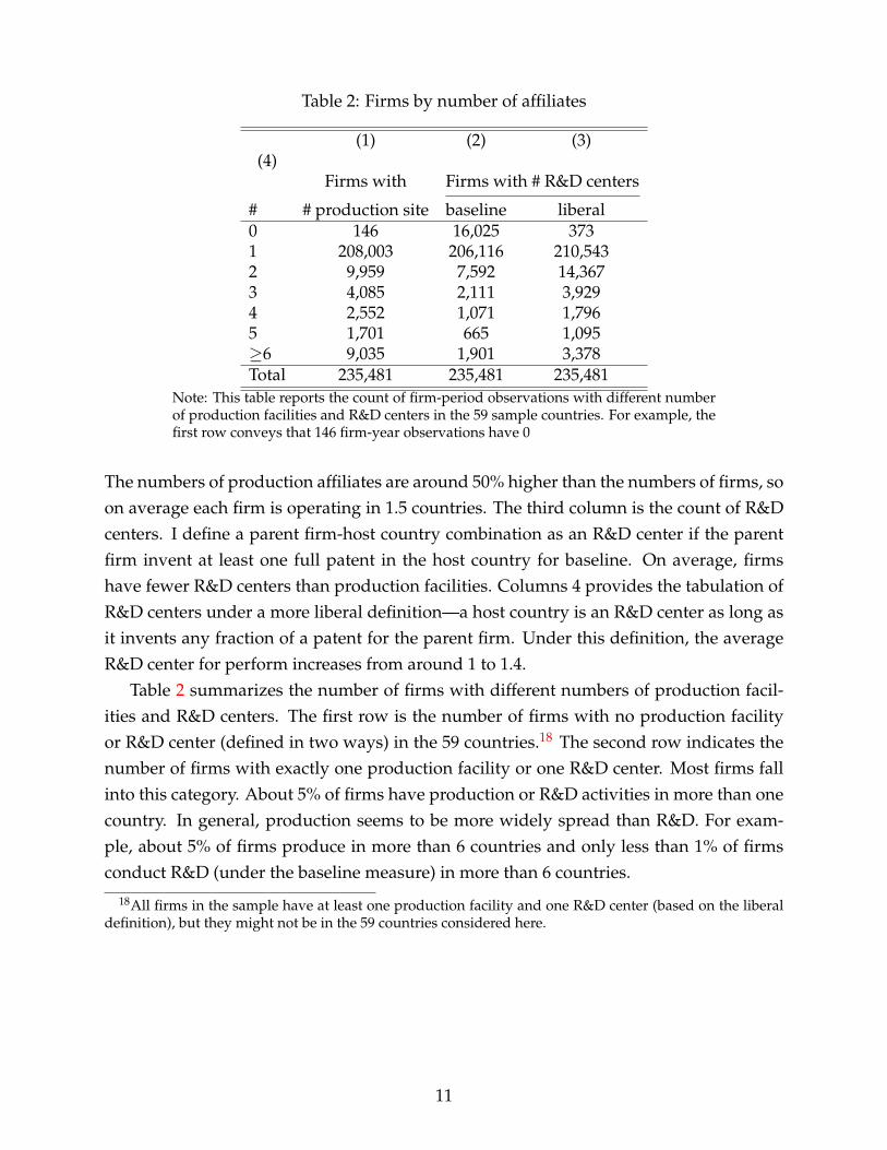
Table 2: Firms by number of affiliates
(1) (2) (3)(4)
Firms with Firms with # R&D centers
# # production site baseline liberal0 146 16,025 3731 208,003 206,116 210,5432 9,959 7,592 14,3673 4,085 2,111 3,9294 2,552 1,071 1,7965 1,701 665 1,095≥6 9,035 1,901 3,378Total 235,481 235,481 235,481
Note: This table reports the count of firm-period observations with different numberof production facilities and R&D centers in the 59 sample countries. For example, thefirst row conveys that 146 firm-year observations have 0
The numbers of production affiliates are around 50% higher than the numbers of firms, soon average each firm is operating in 1.5 countries. The third column is the count of R&Dcenters. I define a parent firm-host country combination as an R&D center if the parentfirm invent at least one full patent in the host country for baseline. On average, firmshave fewer R&D centers than production facilities. Columns 4 provides the tabulation ofR&D centers under a more liberal definition—a host country is an R&D center as long asit invents any fraction of a patent for the parent firm. Under this definition, the averageR&D center for perform increases from around 1 to 1.4.
Table 2 summarizes the number of firms with different numbers of production facil-ities and R&D centers. The first row is the number of firms with no production facilityor R&D center (defined in two ways) in the 59 countries.18 The second row indicates thenumber of firms with exactly one production facility or one R&D center. Most firms fallinto this category. About 5% of firms have production or R&D activities in more than onecountry. In general, production seems to be more widely spread than R&D. For exam-ple, about 5% of firms produce in more than 6 countries and only less than 1% of firmsconduct R&D (under the baseline measure) in more than 6 countries.
18All firms in the sample have at least one production facility and one R&D center (based on the liberaldefinition), but they might not be in the 59 countries considered here.
11

Table 3: Cost of Separating R&D from Production
(1) (2) (3) (4)Dependent variable Production indicator ln (sales)
R&D indicator 0.313∗∗∗ 1.156∗∗∗
(0.003) (0.022)ln (patent count) 0.313∗∗∗ 0.173∗∗
(0.011) (0.078)R2 0.672 0.510 0.565 0.959Within R2 0.048 0.046 0.079 0.004Observations 11889739 139257 27388 20632Firm-period FE Y Y Y YHost-period FE Y Y Y YHome-host FE Y Y YHost-industry FE Y Y YAffiliate FE Y
Note: Columns 1 estimate the effect of having an R&D center on the probability of having aproduction facility in a host country. Conditional on having a production facility in a host, Col-umn 2 estimates the effect of having an R&D center in the same host on the scale of production.Columns 3 and 4 estimate the intensive margin relationship between the size of the R&D centerand the scale of production.Standard errors (clustered at firm level) in parenthesis. ∗ p < 0.10, ∗∗ p < 0.05, ∗∗∗ p < 0.01.
3 Three Facts on Location Choices of R&D and Production
I document three facts on the spatial distribution of R&D and production within a MNC,which collectively highlight the role of geography and talent in the location choice ofMNCs and motivate key ingredients of the model.
3.1 The Cost of Separating R&D from Production
Fact 1: Within a firm, R&D and production tend to be located together.The first fact, reported in Table 3, is on the co-location of R&D and production within
a firm. The first column focuses on the extensive margin and shows that having an R&Dcenter in a country increase the probability of having a production facility in the samecountry by 31%. This estimate is about 10 times the mean value of the dependent vari-able. Column 2 focuses on the relationship between having an R&D center in a host andtotal production in the same country—host country with an R&D center on average hasproduction facilities that are more than 100% larger in sales. Column 3 focuses on theintensive margin for both activities and finds that a 10% increase in the size of the R&Dcenter is associated with 3% increase in the sales of the affiliate. All three specificationscontrol for firm-period fixed effects, so are exploiting within-firm variations across hostcountries. In addition, I control for host-period, home-host, and host-industry (2-digit
12

NACE) fixed effects, to rule out the influence of country or industry specific character-istics, or that affiliates in a host country increase both R&D and production because thehost country economy as a whole grow.
The results so far is supportive of a cost when firms wan to break up production fromR&D, but it can also be driven by the idiosyncratic match quality between a firm and ahost. For example, the technology, human capital, or infrastructures of a country mightbe particularly conducive for some firms because the they fit the technology of the firm,which benefits both R&D and production. To address this concern, Column 4 controlsfor affiliate fixed effect, so it exploits the correlation in over-time changes of productionand R&D output of within an affiliate, controlling on the overall trend of the host countryand the growth of the firm common to all affiliates. To avoid large percentage growth insmall affiliates having a disproportionate impact on the result, I weight the regression bythe square root of the size of an R&D center. The estimated elasticity is around 17%, soaffiliates doing more R&D also see a larger increase in production.
Given the co-location of R&D and production, it might be tempting to think it wouldbe without generality to bundle R&D and production as a composite ‘production’ activityand models MNCs as choosing where to locate this composite activity. Facts 2 and 3 showthat R&D and production of affiliate varies and respond differently to geographic frictionsand other types of country characteristics.
3.2 Headquarter Effects of Affiliate R&D and Production
Fact 2: Both production and R&D in affiliates decrease with distance to the headquar-ters, but at different rates.
The second fact relates R&D and production to various measures of distance betweenthe host country and the headquarters. The literature has documented the activities ofaffiliates in general decreases with distance to headquarters and rationalized this findingusing cost of knowledge transmission and trade costs for input from the headquarters(Yeaple and Keller, 2016; Opromoller et. al). My analysis complements that of the litera-ture by separately investigate the impact on R&D and production.
Table 3 reports the results. In all specifications, I control for firm-period fixed effectsand exclude headquarters from the sample, so the comparison is among affiliates of thesame firm in different countries. I further control for host-industry and host-period fixedeffects so that bilateral variations are not confounded by country or industry character-istics. The first two columns estimate a linear probability model in which the depen-dent variable is an indicator for having a production facility or an R&D center in a hostand the independent variables are measures of distance between the host and the head-
13

Table 4: The headquarter effect on R&D and production
(1) (2) (3) (4)Extensive Margin Intensive Margin
Dependent variable: Production R&D ln (sales) ln (patent count)ln (distance) -0.004∗∗∗ -0.001 -0.255∗∗∗ -0.126∗∗∗
(0.001) (0.000) (0.027) (0.032)Contiguity 0.012∗∗∗ 0.006∗∗∗ 0.198∗∗∗ 0.098
(0.003) (0.002) (0.067) (0.070)Common language 0.008∗ 0.010∗∗∗ 0.257∗∗∗ 0.279∗∗∗
(0.004) (0.002) (0.065) (0.064)Colonial tie 0.016∗∗∗ 0.000 0.213∗∗∗ 0.021
(0.006) (0.003) (0.080) (0.062)R2 0.225 0.095 0.425 0.335Within R2 0.004 0.002 0.014 0.012Observations 11688218 11688218 114150 50135Firm-period FE Y Y Y YHost-industry FE Y Y Y YHost-period FE Y Y Y Y
Note: Columns 1 and 2 estimate the relationship between a host country’s distance distance tothe headquarters and the probability of having a production facility or an R&D center there.Columns 3 and 4 estimate the relationship between distance to headquarters and the size of theproduction facility and the R&D center. Headquarters are excluded from all regressions. Patentcount is weighted by the number of inventors.Standard errors (clustered at country-pair level) in parenthesis. ∗ p < 0.10, ∗∗ p < 0.05, ∗∗∗
p < 0.01.
quarters. The regressions suggest geographic frictions play important but heterogeneousroles. Contiguity and common language are important for both R&D and productionsites, whereas distance and colonial tie matters more for production. The mean value ofthe dependent variable is 0.027 and 0.018, respectively, so the estimated coefficient areeconomically sizable.
Columns 3 and 4 estimate the intensive margin effect between distance to headquar-ters and size of a production facility and an R&D center. The estimates indicator thathaving a common language is important for both activities, but other measures of geo-graphic frictions are in general more important for production than for R&D. Motivatedby this fact, the quantitative model will allows for the two activities to be influenced dif-ferently by geographic frictions.
3.3 The Role of Talent for R&D
Fact 3: Affiliate R&D intensity increases in the quality of human capital of the hostcountry The third fact looks into how the R&D intensity of an affiliate varies across hostcountries. When surveyed about where to locate R&D center, mangers of large multi-
14

Table 5: The Role of Talent in Affiliate R&D Intensity
(1) (2) (3) (4) (5)Dependent variable: ln (patent count/sales)Human capital 0.941∗∗∗ 2.117∗ 3.219∗∗∗ 4.723∗∗∗ 4.757∗∗∗
(0.249) (1.090) (1.199) (1.268) (1.394)IPR protection 0.378 0.263
(0.282) (0.228)R&D subsidies 0.893∗ 0.814∗
(0.468) (0.475)ln (researchers) 0.583∗∗
(0.248)ln (GDP) 0.136 -0.093 0.023 -0.150 -0.515
(0.111) (0.231) (0.388) (0.547) (0.398)ln(GDP per capita) -0.315
(0.251)R2 0.222 0.399 0.697 0.739 0.755Within R2 0.030 0.002 0.012 0.020 0.024Observations 29322 27403 20656 16529 15946Distance measures YFirm-period FE Y Y Y Y YHome-host FE YHost-industry FE YAffiliate FE Y Y Y
Note: The dependent variable is log ratio between patent counts (weighted by number of inven-tors of a patent) and affiliate sales. The first column is a cross-sectional regression that controlsfor firm-period fixed effects and bilateral distance measures (See Table 1 for definition). The sec-ond column controls for time-invariant host characteristics through host-home and host-industryfixed effects. The third to the last columns control for affiliate fixed effects and exploits only over-time variation within individual affiliates.Standard errors (clustered at host-country level) in parenthesis. ∗ p < 0.10, ∗∗ p < 0.05, ∗∗∗
p < 0.01.
national firms frequently rate access to talent as a primary factor (Thursby and Thursby,2005). I examine whether the R&D intensity of an affiliate increases systematically withmeasures of host country talent. Table 5 reports the results. The dependent variable is thelog ratio of affiliate R&D over sales. The independent variables are measures of host coun-try human capital, along with other controls. The first column controls for firm-periodfixed effects and various measures of bilateral distance, so the comparison is within-firm,between host countries. The estimate indicates a significant positive correlation betweenthe R&D intensity of the affiliate and the human capital quality of the country. The sizeand income of the host, on the other hand, does not seems to be important. Columns 2 and3 progressively control for bilateral and host-industry fixed effects, and affiliate fixed ef-fect.19 The result in Column 3 suggests that, as a host country improves quality of human
19This regression exploits overtime variations in human capital of a host country for a given affiliate. Be-cause the overtime changes in GDP and income are highly correlated, I include only one of them. Including
15

capital, affiliates there become more R&D intensive. Column 4 adds IPR protection in-dex and R&D subsidies index, two policy measures likely correlated with R&D. BecauseR&D subsidy data are available for a smaller set of countries, the sample size shrinks.The coefficient for R&D subsidies is marginally significant, but it does not affect the maincoefficient of interest. Finally, in Column 5, I control for the number of researchers. Con-ditioning on the overall human capital, the increase in total number of researchers of acountry is also significantly correlated with the R&D intensity of the affiliate.
To summarize, this section shows that MNCs tend to co-locate their overseas R&Dcenter and production facilities, but the decisions are not the same. Specifically, whileboth types of activities decrease in distance to the headquarters, the decay is faster forproduction than for R&D. The R&D intensity of affiliate in a host country is correlatedwith quality of talent in the host, both in the cross section and overtime. In the appendix,I present various robustness of the three facts using alternative definition of affiliate R&Dand production.
These facts calls for a model of MNCs in which R&D and production are explicitlyintroduced as separate decisions and allowed to depends on differentially on host char-acteristics and geography. In the rest of this paper, I develop such a model to interpret thedata and to quantify the aggregate implications of MNC activities.
4 The model
This section sets up the model and describes firms’ global innovation and operation deci-sions.
4.1 Environment
There are N countries in the model, indexed by i = 1, 2, ...N. Country i is endowed withLR
i measure of researchers, who differ in their talent, θ ∈ Θ, distributed according toHi(θ), and LP
i measure of homogenous production workers.20 Researchers work withR&D centers to develop new differentiated varieties. Production workers manufacturethese varieties and perform operational tasks for R&D centers (in the form of fixed costs).Country i is also endowed with Ei measure of heterogeneous firms with different innova-tion efficiencies, zR ∈ ZR, distributed according to GE
i (zR). Firms build R&D centers in
different countries, which then recruit local researchers to develop new varieties. I use Ri
both does not affect the point estimate for human capital and its statistical significance.20The talent distribution in a country reflects the quality of the education system, education choice, as
well as cultural traits such as openness to innovation. By taking the talent distribution as given, this paperabstracts from the effect of international integration on these factors.
16
to denote the measure of R&D centers in country i. In equilibrium Ri is an endogenousoutcome determined by firms’ offshore R&D decisions.
The representative consumer in country i decides how much to spend on each variety,according to the following preference:
Ui = (∫
Ωi
qi(ω)σ−1
σ dω)σ
σ−1 ,
where Ωi denotes the set of product varieties available in country i, qi(ω) is the consump-tion of variety ω, and σ > 1 is the elasticity of substitution. Let the aggregate consumptionexpenditure in country i be Xi. The demand for variety ω is:
qi(ω) = pi(ω)−σ Xi
Pi1−σ
,
where Pi1−σ =
∫Ωi
pi(ω)1−σdω is the ideal demand price index aggregated over pi(ω),the price of variety ω in country i.
4.2 Firm Decisions: Overview
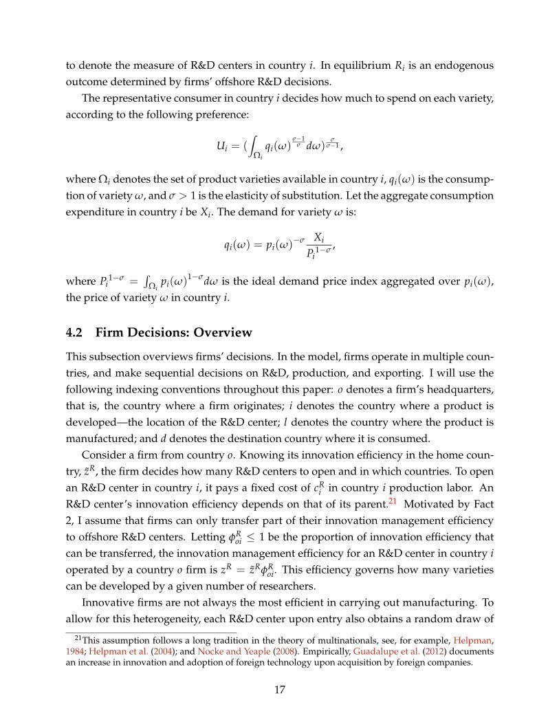
This subsection overviews firms’ decisions. In the model, firms operate in multiple coun-tries, and make sequential decisions on R&D, production, and exporting. I will use thefollowing indexing conventions throughout this paper: o denotes a firm’s headquarters,that is, the country where a firm originates; i denotes the country where a product isdeveloped—the location of the R&D center; l denotes the country where the product ismanufactured; and d denotes the destination country where it is consumed.
Consider a firm from country o. Knowing its innovation efficiency in the home coun-try, zR, the firm decides how many R&D centers to open and in which countries. To openan R&D center in country i, it pays a fixed cost of cR
i in country i production labor. AnR&D center’s innovation efficiency depends on that of its parent.21 Motivated by Fact2, I assume that firms can only transfer part of their innovation management efficiencyto offshore R&D centers. Letting φR
oi ≤ 1 be the proportion of innovation efficiency thatcan be transferred, the innovation management efficiency for an R&D center in country ioperated by a country o firm is zR = zRφR
oi. This efficiency governs how many varietiescan be developed by a given number of researchers.
Innovative firms are not always the most efficient in carrying out manufacturing. Toallow for this heterogeneity, each R&D center upon entry also obtains a random draw of
21This assumption follows a long tradition in the theory of multinationals, see, for example, Helpman,1984; Helpman et al. (2004); and Nocke and Yeaple (2008). Empirically, Guadalupe et al. (2012) documentsan increase in innovation and adoption of foreign technology upon acquisition by foreign companies.
17

Figure 2: Firm’s Two-tiered Decisions
(a) Offshore R&D Decisions
Home Country
o
Innovation Efficiency 𝑧𝑅Host
Country 𝑖1
Retained innovation
efficiency: 𝑧𝑅𝞥𝑜 𝑖1𝑅
Draw production efficiency: 𝑧𝑃from
𝐺𝑃(𝑧𝑃| 𝑧𝑅𝞥𝑜 𝑖1𝑅 )
Host Country
𝑖2
Retained innovation
efficiency: 𝑧𝑅𝞥𝑜 𝑖2𝑅
Draw production efficiency: 𝑧𝑃from
𝐺𝑃(𝑧𝑃| 𝑧𝑅𝞥𝑜 𝑖2𝑅 )
(b) Offshore Production and Export
Host Country
𝑖1
Market 𝑑1
Draw (𝞰1, 𝞰2, 𝞰3, … , 𝞰𝑁),
𝞰𝑙 ∈ 𝐹𝑙(𝑥) = (𝑒−𝑇𝑙𝑥−𝛿)
Production site l
Unit Production Cost: 𝑤𝑙𝑃𝞃𝑙𝑑1
𝑧𝑃𝞥𝑖1𝑙𝑃 𝞰𝑙
18

production management efficiency, denoted zP ∈ ZP, which is common to all productsdeveloped by the R&D center. To capture positive correlation between innovation effi-ciency and production efficiency, the distribution from which zP is drawn increases in zR
in the sense of first-order stochastic dominance. I use GP(zP|zR) to denote the CDF forproduction efficiency draws, with gP(zP|zR) being the corresponding probability densityfunction (PDF).22 This offshore R&D module is illustrated in Figure 2a. As the figure in-dicates, firms can open multiple R&D centers in different countries, but at most one R&Dcenter in each country.
Given the production and innovation efficiency of affiliated R&D centers, (zP, zR),firms recruit researchers in each center to develop new differentiated varieties, and decidewhich countries to sell their products to. To sell products to destination country d, a per-variety fixed marketing cost of cM
d in terms of country d production labor needs to bepaid.
As Figure 2b indicates, firms can potentially manufacture products developed by theirR&D centers in a third country l , where they do not necessarily perform R&D, and thenexport to destination countries. By separating production from R&D (offshore produc-tion), firms can take advantage of cheaper production labor and save on shipping fees.However, geographic separation makes it difficult for R&D centers to communicate withproduction plants, reducing production efficiency. I use φP
il ≤ 1 to denote the fraction ofproductivity that a firm can transfer from its R&D center in country i to production site incountry l. For an R&D center with production efficiency zP, the preserved plant-level off-shore productivity in country l is zPφP
il . I further assume that there is a stochastic element,ηl, idiosyncratic to a production site and a variety, which enters productivity multiplica-tively, so the variety-level productivity in l is zPφP
il ηl. The cost of producing and delivering
one unit of product is wPl τld
zPφPil ηl
, which takes into account the cost of production labor, wPl ,
and shipping fee, τld.In the model, firms perform offshore R&D for several reasons. First, if a country is
relatively abundant in talented inventors, foreign firms might want to enter to make fulluse of their skills. Anecdotes abound about MNCs establishing offshore R&D centers inorder to tap into the local talent pool. Google, for instance, recently announced a planto train two million Android developers in India within the next three years. Accordingto a survey of 200 R&D executives (Thursby and Thursby, 2006), MNCs rank being closeto highly qualified R&D personnel as the most important factor for the location choice ofR&D centers in their home countries and other developed countries, and as the second
22Under this assumption, the production management efficiency is specific to each R&D center. R&Dcenters with different innovation management efficiencies affiliated with the same parent will draw fromdifferent distributions. An alternative interpretation of this production management efficiency is the qualityof products developed by an R&D center.
19

most important factor, right after growth potential, for their new R&D centers in emergingeconomies.
The aforementioned production and trade decisions also imply that firms might chooseto perform R&D in places close to major destination markets, or places with good accessto countries with cheap production labor, in order to produce and distribute their prod-ucts more efficiently.
Importantly, I assume that different varieties developed by a firm, either in the sameor in different R&D centers, are differentiated from each other and from varieties devel-oped by all other firms. This assumption is consistent with how R&D is organized inmany multinational firms. General Electric, for example, organizes its ten research labsby scientific disciplines in five countries (the U.S., Germany, India, China, and Brazil).23
24 This assumption implies that firms make offshore R&D decisions for each country in-dependently and that R&D centers affiliated with the same firm operate as if they areindependent from each other.
Given this independence, in the remainder of this section, I first consider the produc-tion and trade decision of a firm, after a variety has been developed. I then describe theinnovation decision of each R&D center, and firms’ decisions to build offshore R&D cen-ters. Finally, I characterize the market for researchers and analyze the welfare gains fromopenness under a special case.
4.3 Production and Trade
Consider a variety developed by an R&D center (zP, zR) in country i, which can poten-tially be produced in any country by production labor using a linear production tech-nology. For each variety, an R&D center obtains a vector of N idiosyncratic productivitydraws, one for each potential production site, denoted η = (η1, η2, .., ηN). I assume thatηl is independent across countries, and follows a Frechet distribution: F(x) ≡ Prob(η ≤x) = exp(−Λlx−δ), where Λl governs the mean of the draws for country l, and δ governs
23Alternatively, this assumption can be interpreted as capturing M&A FDI. More than 70% of FDI flowsin the data are in the form of mergers and acquisitions (Nocke and Yeaple, 2008). One explanation for thisobservation is that, by transferring know-how and managerial capacity to targets, acquiring firms can im-prove the operating efficiency of the targets. The differentiated-variety assumption adopted in the presentpaper is consistent with this perspective of FDI—multinationals transfer their managerial technology tonewly acquired foreign R&D centers, and increase the efficiency of these R&D centers in carrying out theirindependent product development.
24This assumption treats R&D at headquarters and R&D in offshore centers symmetrically. Recently,Bilir and Morales (2016) estimates the effects of R&D on productivity for multinational firms. They findthat R&D at headquarters have stronger spillover effects to foreign affiliates than R&D at affiliates to otheraffiliates. The current model cannot account for this finding. But an extension of the model that allowsfirms to first invest in R&D to build up "core management capacity" before performing product innovationat home and abroad would be consistent with this finding.
20

the dispersion of the draws across varieties and countries. The productivity for a varietyin country l is: zPφilηl.
Letting wpl denote the wage rate for each unit of production labor in country l, the cost
of serving country d by producing in country l is cild =wp
l τld
zPφpilηl
, where τld is the iceberg
shipping cost from l to d. Given the monopolistic competition market structure, the pricefor a variety sold in country d, if produced in country l, is
pild =σ
σ− 1wp
l τld
zPφpilηl
.
Conditional on serving destination market d, a firm chooses the lowest cost productionlocation for each of its varieties. Because there are no fixed costs in offshore production,all countries are potentially production sites. The price of this variety in country d issimply the lowest one among all possible choices:
pid(η) = minlσ
σ− 1wp
l τld
zPφpilηl.
For each variety and each destination market, production will take place in one country.However, since each R&D center develops a continuum of varieties, in equilibrium, a firmwill serve each destination through all countries in the world.25 For tractability, I assumethat each R&D center needs to decide first which destination markets to enter and paysthe fixed marketing cost before knowing the idiosyncratic country-specific productivitydraws, so firms make destination market entry decisions based on expected profits. Theexpected per-variety profit from market d for the R&D center from country i , defined asπd
i (zP), is
πdi (z
P) =1σ(
σ
σ− 1)1−σΓ(
δ + 1− σ
δ)Pσ−1
d Xd(1zP )
1−σΨσ−1
δid − cM
d wpd ,
where Γ is the Gamma function, and Ψid = ∑l Λl(wp
l τln
φpil)−δ. The first term in this expres-
sion is calculated from 1σ Pσ−1
d Xd∫
minl(pild(η)1−σ)dF(η), with F(η) being the distribution
of η = (η1, η2, ..., ηN).This expected profit increases in the production efficiency of an R&D center, zP, so
there exists a threshold zpid such that R&D centers from i will expend marketing costs and
25This result implies that the model cannot capture the extensive-margin of firms’ offshore productiondecisions. This is not necessarily an important drawback, as the focus of this paper is on offshore R&D andits interaction with offshore production in the aggregate. In the next section I show the model predictionson firms’ offshore R&D decisions are supported empirically.
21

enter country d if and only if their production efficiency is above this threshold. Thiscutoff is given by:
πdi (z
Pid) = 0. (1)
A firm makes an independent entry decision for each destination market. The per-variety expected profit for a firm with production efficiency draw zP, taking into accountits potential entry into all destination markets, is
πi(zP) = ∑d
IzP≥zpid
πdi (z
P). (2)
4.4 Innovation and the Market for Researchers
R&D centers choose the talent of researchers, θ, and their quantity, l(θ), to develop newdifferentiated varieties. Let y be the measure of differentiated varieties developed:
y = f (zR, θ)l(θ)γ,
where γ measures the return to the number of researchers, and f (zR, θ) captures how firminnovation efficiency and researcher talent affect innovation output. I assume that γ < 1,implying decreasing returns to scale in the number of researchers. This assumption hasseveral interpretations. First, it can be thought of as a reduced-form approximation toa model in which R&D requires supervision from the top management, but managerialtime is limited in a company. In such a context, hiring more researchers results in less su-pervision time for each of them, reducing researcher productivity.26 An alternative is tothink of innovation output as a function of both accumulated knowledge capital and re-searcher input. In a static model in which the distribution of knowhow and accumulatedknowledge is given, the research output features decreasing returns to researcher input.Finally, decreasing returns to scale might stem from increases in coordination costs, free-riding, and disagreement among researchers as teams expand.27
Given πi(zP), the per-variety expected profit, the optimization problem for the R&Dcenter is
πRi (z
P, zR) = maxθ∈Θ,l(θ)[πi(zP) f (zR, θ)l(θ)γ − wi(θ)l(θ)],
where wi(θ) is the wage for a researcher with talent θ. As is clear from the equation,the production efficiency of a firm affects innovation incentives because it determines the
26See Antras et al. (2006) for an analysis of the effects of offshoring in a model in which managers canonly supervise a fixed number of workers.
27Such coordination costs have been documented empirically. For example, Haas and Choudhury (2015)finds that, while total patenting increases with the number of members in a team, the increase is smallerthan the increase in the team size—there is decreasing returns in the number of researchers in a team.
22

profit for each variety. I make the following assumption about f :
Assumption 1. f is twice continuously differentiable and increasing in its arguments, i.e., f1, f2 >
0. Further, f is log-supermodular, i.e., ∂2log f (zR,θ)∂zR∂θ
> 0.
The assumption that f1, f2 > 0 simply means that more efficient firms and more ableresearchers are more productive in innovation. The log-supermodularity assumption im-plies strong complementarity between researcher ability and firm efficiency. Under thisassumption, more productive firms have a comparative advantage in working with moreable researchers.28 R&D activities require cooperation between researchers, and a largeamount of managerial and monetary resources. Moreover, after a product prototype isdeveloped, testing and marketing costs are big hurdles to clear before the product canreach consumers. A well-managed firm can do all of these tasks better, so it is especiallyprofitable for them to work with talented researchers. The model captures this idea withthe log-supermodularity of f .
The setup here deviates from the efficiency units assumption. A researcher with hightalent is more valuable than multiple researchers with lower talent. Similarly, a firm withhigh innovation efficiency is more productive in R&D than multiple firms with lower ef-ficiencies. These implications are in line with a few observations in the literature. First, asmentioned earlier, the quality of research talent is one of the top considerations when firmschoose where to build their offshore R&D centers, along with the cost of research labor.29
Second, it is well documented that there are a large number of small and less produc-tive firms in developing countries, the prevalence of which can account for an importantfraction of cross-country income differences (Hsieh and Klenow, 2009). Management effi-ciency might be a source of performance differences between firms (Bloom et al., 2013). Tothe extent that many developing countries have a large number of very small firms, theymight not necessarily the lack a sufficient stock of management efficiency. The model hereis consistent with view that it is not necessarily lack of management efficiency stock, butrather the lack of exceptional firms like Apple and Google, that explains the low incomesin developing countries.30 Finally, the complementarity also implies that the same inven-tor will be paid more to work in a more efficient firm. This is consistent with the finding
28The log-supermodularity assumption has been adopted in a growing literature in international tradewhich uses assignment models to study questions such as the determinants of specialization and the im-pacts of trade integration, as reviewed recently by Costinot et al. (2015). The framework here is similar tothe one in Grossman et al. (2017).
29Branstetter et al. (2013) conducts interviews with foreign-affiliated R&D centers in China. The interviewresponses stress the scale and quality of the research talent in China, rather than its cost.
30Roys and Seshadri (2014) builds a model of matching between heterogeneous entrepreneurs and work-ers, enriched with human capital accumulation, to show that the model can account for the differences inlife cycle dynamics between firms in rich and poor countries, and can explain a substantial share of incomedifferences between countries.
23

that larger and more productive firms pay a wage premium (see, for example, Schank etal., 2007), and the evidence on positive assortative matching between firms and inventorsI provide in the appendix.
I now characterize the market for researchers. Let Ti(zP, zR) : (ZPi , ZR
i ) → Θ be theoptimal choice of θ for an R&D center characterized by (zP, zR). We have the followinglemma:
Lemma 1. Ti is continuous and strictly increasing in zR. Moreover, Ti is independent of zP.
Proof. See appendix.
The proof of Lemma 1 is an extension of assortative matching results in the literature(see, for example, Grossman and Helpman, 2014; Grossman et al., 2017; Sampson, 2014)to the case with an additional source of heterogeneity, namely the production efficiency.Because high zR R&D centers enjoy a higher marginal productivity increase from hir-ing better researchers, they have a comparative advantage in working with high-abilityresearchers, leading to assortative matching. Since zP enters firms’ innovation outputmultiplicatively in the form of πi(zP), higher zP does not affect the type of researchershired by an R&D center, but only their quantity. In the following I will write the matchingfunction simply as Ti(zR), omitting the argument zP.
Given the equilibrium wi(θ), the demand of an R&D center for researchers, if it choosesresearchers with talent θ, is
li(zP, zR) = (γπi(zP) f (zR, θ)
wi(θ))
11−γ . (3)
The corresponding measures of invention and profit are therefore:
yi(zP, zR) = (γπi(zP)
wi(θ))
γ1−γ f (zR, θ)
11−γ , (4)
πRi (z
P, zR) = (γγ
1−γ − γ1
1−γ )wi(θ)− γ
1−γ [πi(zP) f (zR, θ)]1
1−γ . (5)
In equilibrium, firms choose the type of researchers to maximize profit. This requiresthe improvement in marginal output from higher-quality researchers to be exactly offsetby their higher wages. We can obtain this equation by differentiating Equation (5) withrespect to θ:
Lemma 2. wi(θ) satisfies the following relationship:
w′i(θ)wi(θ)
=f2(zR, θ)
γ f (zR, θ)|θ=Ti(zR). (6)
24

Proof. See appendix.
The formal proof of Lemma 2 establishes the differentiability of wi(θ). The proof issimilar to that in Sampson (2014) and is delegated to the appendix.
Since researchers are heterogeneous, labor market clearing requires that the total de-mand equals total supply for each type. Let θi and θi be the lower and upper limits of thesupport for the researcher talent distribution, and let zR
i and zRi denote the lower and up-
per limit of the support for the innovation efficiency distribution, respectively. To derivethe researcher market clearing conditions for each type, I start with an aggregate version:for all θi < θ < θi, the number of researchers with talent lower than θ is equal to the totaldemand for researchers with talent below θ. Formally,
LRi
∫ Ti(zR)
θi
dHi(θ) = Ri
∫ zR
zRi
[∫
ZPli(zP, z)gP
i (zP|z)dzP]gR
i (z)dz
= Ri
∫ zR
zRi
(γ f (z, Ti(z))
wi(Ti(z)))
11−γ [
∫Zp
πi(zp)1
1−γ gPi (z
P|z)dzp]gRi (z)dz,
where Ri is the measure of R&D centers in country i and gRi (z) is their PDF, both of
which are determined in equilibrium by firms’ offshore R&D decisions. On the left ofthis equation is the total number of researchers with talent below Ti(zR), and on the rightside is the corresponding total demand.
Differentiating this equation with respect to zR, we have the following equation:31
LRi T′(zR)hi(Ti(zR)) = Ri(
γ f (zR, Ti(zR))
wi(Ti(zR)))
11−γ
∫ZP
gRi (z
R)πi(zP)1
1−γ gP(zP|zR)dzP (7)
Equation (7) then characterizes the market clearing condition for each researcher type.Equations 6 and 7, together with two boundary values,
Ti(zRi ) = θi, Ti(zR
i ) = θi, (8)
determine the matching function Ti(zR) and the wage schedule wi(θ). In summary, wehave the following results:
Proposition 1. Under Assumption 1, 1) Firms with higher innovation efficiency hire strictly bet-ter researchers. Firms with the same innovation efficiency but different production efficiencies hire
31Because of offshore R&D decisions, gRi is not necessarily continuous. At the finite discontinuous points
of gRi , the matching function might not be differentiable. In this case, Equation 7 is not defined on the dis-
continuous points of gRi . While Ti is still well defined and continuous, the kinks in T′i make it challenging to
solve the matching function numerically. In the quantitative section, I describe a computational algorithmsuited for this context.
25

the same type of researchers in different quantities. 2) The researcher labor market is characterizedby Equations 6, 7, and 8.
4.5 Offshore R&D
Now we can characterize firms’ decisions to open offshore R&D centers. I make the fol-lowing assumption about gP(zP|zR).
Assumption 2. The distribution from which an R&D center draws its production efficiency zP
increases in the innovation efficiency of the R&D center in the sense of first-order stochastic dom-inance.
Define πRi (z
R) as the expected profit (over the possible zP draws) for an R&D centerin country i, with innovation efficiency zR:
πRi (z
R) =∫
ZPπR
i (zP, zR)gP(zP|zR)dzP
Firms compare the expected profit from building an offshore R&D center to the fixedcost of setting up the center, cR
i wPi . By definition (Equations 5 and 2) , πR
i (zP, zR) increases
in zP. We can also show that πRi (z
P, zR) increases with zR.32 Assumption 2 then impliesthat πR
i (zR) increases strictly in zR, so the decision to offshore R&D follows a threshold
rule: there exists a cutoff zRoi, so that firms from country o will perform offshore R&D in
country i if and only if its innovation efficiency is above zRoi. This cutoff is given by the
following zero profit condition:
πRi (z
Roiφ
Roi) = cR
i wPi . (9)
4.6 R&D Center Efficiency Distribution
Firms’ offshore R&D decisions determine gRi , the distribution of innovation management
efficiency, and hence the distribution of production management efficiency, in each coun-try. Given zR
oi, we can now derive R&D centers’ production and innovation efficiencydistributions. Let GR
i (zR) be the CDF for innovation management efficiency of the R&D
centers active in country i, and let GEo (zR) be the CDF of the distribution of innovation
efficiency for firms from country o. Then we have the following equation:
RiGRi (z
R) =N
∑o=1
I zR
φRoi>zR
oiEoGE
o (zR
φRoi)
32From Equation 5, ∂log(πRi (z
P ,zR))
∂zR |θ = Ti(zR) =1
1−γ∂log( f (zR ,θ))
∂zR > 0.
26

Differentiating this equation with respect to zR, we obtain the density function:
gRi (z
R) =1Ri
N
∑o=1
I zR
φRoi>zR
oiEogE
o (zR
φRoi)
1φR
oi. (10)
The PDF for R&D centers with (zP, zR) is gi(zP, zR) = gP(zP|zR)gRi (z
R).
4.7 Aggregation
Knowing gi(zP, zR), I derive the total measure of varieties that are invented in a country,denoted Mi, and the distribution of these varieties over different production efficiencies.Letting mi(zP) be the measure of varieties innovated in country i by R&D centers with aproduction efficiency of zP, then we have:
mi(zP) = Ri
∫ZR
yi(zP, zR)gi(zP, zR)dzR
Mi =∫
ZPmi(zP)dzP,
(11)
where yi(zP, zR) is given by Equation 4. The price index in country d is then given by thefollowing equation:
P1−σd = ∑
i
∫zP>zp
id
mi(zP)[∫
minlpild(η)1−σdF(η)]dzP
= Γ(δ + 1− σ
δ)(
σ
σ− 1)1−σ ∑
iΨ
σ−1δ
id
∫zP>zp
id
mi(zP)zPσ−1dzP
(12)
To express the aggregate objects in the model, let Xid be the total sales in country d ofthe products developed in country i. We have the following:
Xid = Pσ−1d Xd
∫ ∞
zPid
mi(zP)[∫
minlpild(η)1−σdF(η)]dzP
= (σ
σ− 1)1−σΓ(
δ + 1− σ
δ)Pσ−1
d XdΨσ−1
δid
∫ ∞
zPid
mi(zP)(zP)σ−1dzP.(13)
These sales can be fulfilled through production in any country. Letting Xild denote thevalue of production in country l, then we have ∑l Xild = Xid. I further define Yl to be thetotal production of the varieties in country l, so ∑i,d Xild = Yl. The Frechet assumption onidiosyncratic productivity draws also implies that, for each R&D center located in countryi, the share of products it sells in country d that are fulfilled through production in country
27

l is:
ψild =Λl(
wPl τldφP
il)−δ
Ψid,
with Ψid = ∑l Λl(wp
l τld
φpil)−δ. Because this probability is the same for all R&D centers from
country i, it also applies to the aggregate sales:
Xild = ψildXid. (14)
Production workers are used to produce output, and to pay fixed R&D and marketingcosts. The production labor market clearing condition is:
wPd LP
d =σ− 1
σYd︸ ︷︷ ︸
Production
+∑o
EocRd wP
d (1− GRo (z
Rod))︸ ︷︷ ︸
Fixed R&D center setup costs
+ cMd wP
d ∑i
∫ ∞
zPid
mi(zP)dzP
︸ ︷︷ ︸Fixed marketing costs
. (15)
Recall that the density of firms from country o with innovation efficiency zR is gEo (zR).
We can integrate πRi over gE
o (zR) to compute the total profits made by country i R&Dcenters affiliated to firms from country o, denoted Πoi:
Πoi = Eo
∫ zRi
zRoi
πRi (z
RφRoi)gE
o (zR)dzR,
This profit is after deducting R&D, marketing, and production costs, but before de-ducting fixed costs for building R&D centers.
Let Ii be the total R&D expenditures in country i, defined as total compensation toresearchers in country i. Let Ioi be the expenditures in Ii that are incurred by affiliates offirms from country o. Equations 3 and 4 imply that:
Ii = ∑o
Ioi =γ
1− γ ∑o
Πoi
The income of country d comes from three sources: wages of production labor, com-pensation to researchers, and the net profit made by domestic firms from the country.Current account balance requires that total consumption of each country equals total in-come:
Xd = wPd LP
d︸ ︷︷ ︸Production Labor
+∑i[Πdi − EdcR
i wPi (1− GR
d (zRdi))]︸ ︷︷ ︸
Net Profit
+ Id︸︷︷︸Researcher Compensation
. (16)
Definition 1. The competitive equilibrium is defined as a set of allocations and prices, such that
28

all firms optimize, all markets clear, and all firm level decisions are consistent with aggregateallocations and prices (See Appendix for detail).
4.8 The Gains from Openness
In this subsection I focus on a special case to derive an expression for the welfare gainsfrom openness, defined as the percentage change in real income ( Xd
Pd), as a country moves
from complete isolation to the degree of openness observed in the data. This expressionmakes it clear that offshore R&D is a new channel for countries to benefit from globaliza-tion. It also relates the size of this benefit to observable information and model parame-ters. Specifically, I make the following assumption:
Assumption 3. 1) f (zR, θ) = zRθβ;2) Production efficiency, zP, is independent of zR, and follows a Pareto distribution: GP
d (x) =
1− ( xzP
d)−κP ;
3) There is no fixed marketing cost: ∀d, cMd = 0;
4) Firm innovation efficiency, zR, follows a Pareto distribution: GEd (x) = 1− ( x
zRd)−κR .
The first part of the assumption maintains that f (zR, θ) takes a multiplicative form.33
Under this assumption, ∂2log f (zR,θ)∂z∂θ = 0, so f (zR, θ) no longer satisfies the strict log-
supermodularity requirement in Assumption 1. Since a CES function with elasticity ofsubstitution smaller than 1 satisfies strict log-supermodularity, the multiplicative caserepresents the limiting case as the elasticity approaches 1. This simplification will allowus to solve for the equilibrium wage schedule and firm-level decisions analytically.
In the general model, because firms endogenously choose how many varieties to de-velop, aggregation is difficult. The first three components of Assumption 3, however,imply the Pareto distribution of production efficiency for varieties, which admits analyti-cal aggregation. The fourth component in turn allows us to derive the total fixed costs ofR&D in each country. With these simplifications, we have the following:
Proposition 2. Under Assumption 3, the gains from openness for country d, defined as the per-centage change in Xd
Pdas a country moves from complete isolation to the observed equilibrium,
is
GOd = (Xddd
∑l Xdld)−
1δ (
∑l XdldXd
)−1
σ−1 (IddId
)−1−γσ−1 (
σ−1σ
σ−1σ
YdXd
+ (1−γ)κR−1γκR
IdXd(1− Idd
Id))− 1. (17)
Proof. See appendix.
33The assumption that the power of zR is 1 is without loss of generality, because the units of zR can alwaysbe scaled so that it enters f (zR, θ) with a power of 1.
29

This expression highlights various forces through which a country benefits from eco-nomic integration. The first term, Xddd
∑l Xdld, captures the benefits from offshore production
for consumption. The second term, ∑l XdldXd
, captures the benefits from foreign innovationfor consumption. These two terms are direct effects of offshore production and trade inthe model. The third term, Idd
Id, captures the importance of foreign firms in domestic R&D.
Intuitively, the smaller is this ratio, the more a country relies on foreign affiliates for R&D,and the more significant are the welfare gains from offshore R&D. The last term in theequation captures the effects of profit flows on welfare through their impacts on total ex-penditures. This indirect effect tends to bring positive welfare impacts, for countries thatspecialize in R&D (smaller Yd
Xd), and countries that rely more on domestic firms in R&D
(smaller Id−IddXd
).34
In the appendix, I compare this formula to that from Arkolakis et al. (2018). The firsttwo and the fourth terms in Equation 17 also appear in their formula, with minor adjust-ments to reflect the modeling differences. The third term, Idd
Id, does not show up in their
formula. To have an idea of how large this term is, consider the median country in thequantitative section, with about 30% of its R&D done by foreign affiliates. The value of( Idd
Id)−
1−γσ−1 is around 1.055, when γ = 0.4 and σ = 5. All else equal, this term generates
a 5% real income change. So offshore R&D indeed represents a quantitatively importantchannel through which countries benefit from global integration.
5 Parameterization
I now perform a quantitative analysis of the model outlined in Section 3. I focus on asample with 25 countries and a statistical aggregation of another 22 countries.35 I pa-rameterize the model to be consistent with the data in its predictions on the interna-tional interactions between countries and the size distribution of firms within the U.S.This section describes the parameterization procedures, starting with the functional formassumptions.
5.1 Additional Assumptions
In the quantification, I embed an occupational choice into the model. Throughout therest of the paper, I assume that each country is endowed with Li number of workers, withtalent distribution Hi(θ). Workers sort into production labor or research. Each productionworker has one unit of production labor, and each researcher has θ units of talent in
34Finite aggregate fixed R&D costs require (1− γ)κR − 1 > 0.35The list of countries in this statistical aggregation is provided in the appendix.
30

research. Adding occupational choice generates endogenous responses in the supply ofinventors in counterfactuals experiments.
The function f (zR, θ) determines the complementarity between the innovation man-agement efficiency of firms and the talent of researchers. I assume that f is a CES functionwith elasticity of substitution α < 1:
f (zR, θ) = (zRα−1
α + θα−1
α )α
α−1 .
This specification satisfies the log-supermodularity assumption. As α approaches 1, thecomplementarity between researcher talent and firm efficiency weakens.
The distributions of worker talent and firm innovation efficiency are parameterized tobe truncated Pareto distributions, given below:
Hi(θ) =(θ−κθ
ii − θ−κθ
i )
(θi−κθ
i − θi−κθ
i ), GE
i (zR) =
(zRi−κR
i − zRi−κR
i )
(zRi−κR
i − zRi−κR
i ).
In these expressions, the letters with upper and lower bars indicate the upper and lowerbounds for their respective distributions. κR
i and κθi are the truncated-Pareto counterparts
to the shape parameter in the Pareto distribution.To capture the correlation between innovation and production efficiency at the firm
level, I assume that there are two distributions, indicated by H and L (for high and low,respectively), from which firms draw their productivity zP. The probability of drawingfrom the high distribution depends on a firm’s innovation efficiency in the following fash-ion:
Prob(zP ∈ H|zR) =exp(A + B× zR)
1 + exp(A + B× zR), (18)
where A and B are parameters to be estimated. A positive value for B means that moreinnovative firms tend to be more productive as well. H and L are both Pareto distributionwith the same shape parameter κP:
GH(zP) = 1− (zP
HzP )κP , GL(zP) = 1− (
zPL
zP )κP .
I assume that zPL < zP
H, so the H distribution first-order stochastically dominates the Ldistribution.
31

5.2 Parameters Assigned Directly
I set the number of workers in a country, L, to total employment from the Penn WorldTables. To focus on differences in the firm efficiency distributions and to abstract from thedifferences in the number of firms, I set E, the measure of firms, to be proportional to L.This proportion is chosen so that the average employment per firm in the model equalsthe average employment per firm in the U.S.
I directly assign values to a few parameters in the model. Parameter σ, the elastic-ity of substitution between varieties, determines the markup charged by firms. I set thisparameter to be 5, following recent studies in international trade (see Simonovska andWaugh, 2014, for example). This value also implies that 20% of sales are variable prof-its. In the U.S., R&D expenditures account for about 8% of manufacturing sales. Themodel counterpart of R&D expenditures is researcher compensation. I set γ, the shareof researcher compensation in variable profit, to 0.4, so that researcher compensation ac-counts for about 8% of sales in the model.
Equation 14 implies log(Xild) = αid + βil − δlog(τld), where αid and βld are pair fixedeffects. δ therefore determines the elasticity of Xilds with respect to the cost of shippingfrom l to d. Based on Arkolakis et al. (2018), which estimates this specification using theaffiliate production and sales data of U.S. multinationals (i = U.S.), I set δ to 10.9.
Calibrating firm efficiency and worker talent distributions for each country requirescomparable data across countries. I use the World Management Survey by Bloom et al.(2012) and the cognitive test score data by Hanushek and Woessmann (2012) to calibratethese distributions.
The World Management Survey provides firm-level management scores for each coun-try in the sample. In the survey, interviewers rate each firm based on its talent manage-ment policy and production efficiency along various dimensions. The overall manage-ment score for a firm is then averaged over these sub scores. The talent managementscore intends to capture whether firms follow good managerial practice for retaining andincentivizing its talent, so it is closely related to whether a firm is able to make full useof its research talent. I use it to calibrate innovation management distributions. I obtainthree distribution statistics of zR for each country: mean, standard deviation, and disper-sion.
I use firm-level talent and production management scores to estimate A and B, thecoefficients linking a firm’s innovation and production efficiencies. Specifically, I classifya firm as being from a high productivity distribution if its production management scorefalls into the top 1% of the distribution in the world (the top 4% in the U.S.). I then estimatethe relationship between a firm’s innovation management score and the probability that
32

Table 6: Parameters Calibrated Externally
Symbol Descriptions Value Source
σ Elasticity of substitution between varieties 5 Simonovska and Waugh (2014)γ Return to research team size in R&D 0.4 Manufacturing R&D shareδ Dispersion in offshore production efficiency draws 10.9 Arkolakis et al. (2018)A Probability of having a high production efficiency -6.3 EstimatedB Dependence of zP on zR 0.17 Estimated
it is from a high productivity distribution using the Logit model given by Equation 18.This procedure determines A = −6.3, B = 0.167.36
For the talent distribution, I obtain average cognitive score and the share of studentsreaching “basic” and “top” performance from the test score database, which are definedbased on a common absolute level across countries. To pin down the relative scale ofmanagement efficiency and talent, I take the U.S. as the benchmark. Specifically, I setHUS(θ) and GR
US(zR) to be the same, and use the three statistics on the talent management
score to pin down all three parameters in GRUS(z
R).37 I then determine the distributionsfor other countries, by relating their distribution statistics to those of the U.S.38
Table 6 summarizes the information on the parameters determined directly. I chooseadditional parameters jointly in equilibrium, a process I describe below.
5.3 Parameters Determined in Equilibrium
Overview The remaining parameters to be determined include international frictions,τld, φR
oi, φPil, cM
d , and cRi ; country-specific productivity, Λl; production effi-
36The choice of the top 1% cutoff is motivated by the importance of the most productive firms in inter-national business and in production in general. A high cutoff allows me to better capture the distributionof the very top firms. The implicit assumption underlying this calibration strategy is that firms drawingtheir production efficiency from the L distribution constitute the bottom 99% in the production efficiencydistribution, whereas firms drawing from the H distribution constitute the top 1% of production efficiency.This assumption does not hold exactly because under the Pareto assumption, GL(zP) will always overlapwith GH(zP). Given the choice of the cutoff (1%), however, the calibrated ZP
H will be large enough so theoverlap is negligible.
37The talent management score is approximately normal in the data. Since it is well known that thefirm size distribution has a fat tail, I take the exponential of original scores and use that to match firms’innovation efficiency distribution. The statistics I use to pin down each country’s distribution are basedon these exponents of scores. A few countries in the quantitative analysis are not covered by the WorldManagement Survey. I impute their statistics based on country characteristics. The calibration appendixreports the procedures used in the imputation process.
38For firm innovation distributions, the three moments can be perfectly matched by the three parametersin the truncated Pareto distribution. For the talent distribution, however, the truncated Pareto distributioncannot perfectly match all three moments. I therefore use only the average score and the top student shareto pin down the upper bound and the shape parameter, while setting the lower bound to be the sameacross countries. This simplification, however, does not leave out important information, as the correlationbetween the share of students reaching basic performance and the average score is 0.92.
33

ciency distribution parameters, zPL , zP
H, and κP; and complementarity between manage-ment and talent, α. Although in equilibrium these parameters are jointly identified, forcertain parameters some moments are more informative than others. I describe belowhow each parameter is determined.
The iceberg components of international frictions, τld, φRoi, and φP
il, determinethe aggregate flows of international integration. I use them to match bilateral trade shares,offshore R&D shares, and offshore production shares. The data sources for these bilateralrelationship include: the multinational production data sets introduced in Ramondo etal. (2015); bilateral trade including domestic absorption from the World Input-OutputDatabase; and bilateral offshore R&D information based on patenting statistics at USPTOfrom the OECD patent database. To reduce measurement errors, I average the bilateralpatenting and trade data over the period of 1998-2007.39
The fixed components of international costs, cMd and cR
i , determine the extensivemargin of firms’ global operation. Due to lack of this information for a large sample ofcountries, I assume that these fixed costs are the same for all country pairs, and choosethem to match the share of exporters (0.35) and the share of foreign affiliates among re-search active firms (0.037) in the U.S. manufacturing sector, respectively. I calibrate Λl,the labor productivity in production, by matching the real per-capita income of each coun-try.
I normalize zPL to 1, and determine α, zP
H, and κP jointly. α affects both the patternof matching between firms and researchers, and the firm size distribution. Strong com-plementarity (small α) puts efficient firms at an advantage in working with talent, whichaffects the shape of the matching function and the concentration of researchers. Figure 3aplots the model matching function under various α. The matching functions correspond-ing to smaller α tend to be more convex, with a larger share of researchers working forthe top firms.40 I measure the overall convexity of the matching function using the ratiobetween the average slope of the matching function for the top 50% zR firms, and theaverage slope for the bottom 50% firms. This convexity conveys information about thevalue of α, and will be used as a calibration target. I discuss below how I construct themodel and empirical measures for this convexity.
By determining the distribution of talent across firms, α also affects the number ofproducts a firm develops, and hence the firm size distribution. Numerically, it is mostlyinformative about the size of firms in the top 1%. In addition to α, κP and zP
H are alsoimportant about the firm size distribution: κP directly affects the Pareto shape of the firm
39The multinational production database is averaged over 1996-2001 in the original source.40From Equation 7, other things equal, the slope of the matching function reflects the size of the research
teams. The steeper the curve, the larger is the research team. A more convex matching function thus meansa more unequal distribution of research team size, similar to the Lorenz curve.
34

Figure 3: The Model and Empirical Matching Function
(a) Model matching function (b) Empirical and “noisy” model matching function
Notes: In both panels, the horizontal axis plots percentiles of firm innovation efficiency, and the vertical axis plots percentiles ofresearcher talent. The upper panel is the model matching function under different α. The lower panel shows the empirical matchingfunction estimated by the author using the USPTO data (solid line), and simulated “noisy” model matching functions under differentα.
size distribution at the very top, while zPH effectively determines the scale of the top 4%
firms relative to the bottom 96%, as about 4% of U.S. firms draw from the H distribution.Specifics about the matching function I estimate parameters of matching function
based on the test of positive assortative matching between inventors and firms, pre-sented in Appendix C.4.1. Specifically, I measure firm innovation efficiency using theper-inventor innovation output, and inventor talent using past innovation. Focusing on asample of job switchers, I then estimate nonparametrically how the talent of an inventoris related to the innovation efficiency of the new firm, controlling for inventor and firmcharacteristics as well as time and patent category fixed effects. A positive correlationindicates positive assortative matching. The solid line in Figure 3b presents the estimates,along with a 2 s.e. band. The overall convexity measure of this empirical matching func-tion is 1.71.
We cannot directly compare the model convexity measure to its data counterpart. Inthe data, matches are noisy, so the range of the estimated matching function is not [1, 100],whereas in the model, this is always the case. To make the two comparable, I take thestand that in choosing the optimal types of researchers, firms make mistakes. They cannotdifferentiate workers whose talent satisfies firms’ first order condition (Equation 6) withina certain “error margin”. I fix the wage schedule at the benchmark equilibrium, and thenchoose the size of this margin so that the estimated matching function using simulateddata has the same range as the empirical matching function. I then compute the convexity
35

Table 7: Fit of the Targeted Moments
Parameter Value Moments Model Data
cM 0.0693 Share of exporters 0.35 0.35cR 2.6 Share of foreign affiliates 0.042 0.037
zPH, α, κP
zPH = 1.2 Fraction of firms with emp.<100 0.99 0.99
α = 0.7 Fraction of firms with emp.<20 0.95 0.95κP = 8.16 Matching function slope between 0%-50%/ slope between 50-100% 1.58 1.71
Share of emp. in firms with>500 emp. 0.41 0.47Power law coefficient of firm size dist. 1.04 1.05
measure based on this simulated matching function.41
Figure 3b plots the simulated noisy matching function when α is 0.7, which will be thebenchmark calibration, and two different values. The benchmark value offers the best fitfor the overall concavity, determined by the value of the matching function at the 50thfirm percentile. A smaller α could fit the overall shape reasonably well, but misses the toprange. A larger α, on the other hand, is a poor fit overall.
5.4 Computational Algorithm
A detailed account of the computational algorithm is provided in the appendix. Thissection briefly describes the nested procedure I use. In the outer loop, I choose zP
H, κP,cM, cR, and α to match the targets described above. In the middle loop, I iterate over τ,φR, φP, and T to match all bilateral shares and per-capita real income of countries.The inner loop solves the model given exogenous parameters.
This computation algorithm requires solving the researcher market equilibrium for allcountries at different parameter values. With offshore R&D decisions in the model, thedistribution of R&D center innovation efficiency, gR
i (zR), is an endogenous outcome. The
cutoff rule in offshore R&D decisions implies that gRi (z
R) could have multiple disconti-nuities. As a result, the matching function, Ti(zR), is not necessarily differentiable. In thiscase, general boundary value problem solvers routinely fail or takes a long time to findthe solution. In the appendix, I develop a computational algorithm that is well-suited forthis exercise.
36

5.5 Goodness of Model Fit
The calibration process determines that cM = 0.069, cR = 2.6, zPH = 1.2, κP = 8.16, and
α = 0.7. Table 7 reports the value of parameters and the model moments that help pindown these parameters. Overall, the model is able to fit data along these dimensionswell. To validate the model, I present additional implications of the model under thebenchmark calibration and compare them to the data.
The management score difference between large and small firms The calibrationprocedure for κP and zP
H takes the stand that management efficiency differences are thefundamental cause of performance differences among firms.42 To validate this assump-tion, I examine the model’s performance in matching the mapping from managementscore to firm size. This is a valid test because the calibration uses the information onmanagement scores and the firm size distribution separately, but puts no restrictions onhow a one-point increase in the management score at different percentiles of the firm sizedistribution translates into increases in firm size. For this comparison, I use the total man-agement score, defined as the sum of the innovation and production score, for a consistentcomparison with the empirical evidence.
The first panel of Table 8 reports the difference in total management score betweenfirms with 10000 employees and firms with 10 employees for the model and data.43 Inthe model, the difference in total management score between an average firm with 10000employees and an average firm with 10 employees is 1.18 times the standard deviation ofthe management score, which is close to the empirical counterpart of 1.32.
Figure 4 plots nonparametrically the relationship between management score and firmsize from the model and the data. The estimated curve from the data, in the left panel,displays some convexity: initially, firm size increases relatively slowly with managementscore; at the top range, however, a small increase in management score results in a largerpercentage increase in firm size. Such a relationship can always be captured by the modelby choosing how management score scales into productivity, which is partially deter-mined by zP
H. The question is whether the scale chosen to match other moments is ableto generate this relationship. The right panel is the model relationship between manage-
41For different α, the size of the “error margin” needed to match the range of the empirical matchingfunction varies. But as long as α < 1, the simulated matching function can always match the range ofits empirical counterpart. When α approaches 1, firms become increasingly indifferent between differentresearchers. A small amount of mistakes in recruiting would then result in a flat matching function.
42The calibration essentially takes the management score distribution from data, and chooses κP and zPH
so that the variation in firm size is close to that in the data.43The empirical counterpart of this number is from Bloom et al. (2014), which estimates this relationship
nonparametrically, focusing on medium-sized U.S. manufacturing firms with 10-10000 employees. Becausethe two surveys have different scales for scoring, I normalize the increase by the standard deviation of totalmanagement score.
37

Table 8: Additional Untargeted Moments
Management Score and Firm Size Model DataManagement score difference between large and small firms 1.18 1.32
The Management Efficiency of Foreign AffiliatesForeign affiliate advantage 1.33 1.16Coefficient of variation across countries 0.094 0.075Correlation with domestic average score -0.67 -0.84
Figure 4: Management Score Difference Between Large and Small Firms
(a) Data (b) Model
Notes: The left panel shows the model relationship between management score and firm employment in the data estimated in Bloomet al. (2014); the right panel shows the model counterpart. Both are based on the sub-sample of firms with employment between 10and 10000. The range of variation in x-axis is 1.18 times the standard deviation of the management score in the data, and 1.32 in themodel.
ment score and employment. Consistent with the data, the model also generates someconvexity.
The multinational managerial advantage One important assumption of the modelis that affiliates’ innovation efficiency depends on that of their parents, rather than thatof host country domestic firms. This assumption, together with the self-selection mecha-nism, implies that foreign affiliates tend to be more management efficient than domesticfirms, and that the managerial advantage of foreign affiliates is larger in countries withworse domestic innovation management efficiency.
38

Figure 5: Share of R&D in Income: Model versus Data
Notes: This figure plots the share of income from non-production labor in the model against the share of R&D in GDP in the dataacross countries. The measure for the U.S. is normalized to have 1 in both the model and the data.
I validate these implications quantitatively by calculating the foreign affiliate manage-rial advantage for each country. The measure I use is the ratio between average foreignaffiliate innovation efficiency and average domestic firm innovation efficiency, . I thencompare the statistics of this measure among the sample countries to their data counter-part, constructed using the database introduced in Bloom et al. (2012).
The bottom panel of Table 8 reports the statistics of the foreign affiliate managerialadvantage for the sample countries. Both the model and the data indicates a larger inno-vation management score for foreign affiliates compared to domestic firms, although thedifference is larger in the model (33%) than in the data (16%). The variability of the for-eign affiliate advantage measure across countries, captured by its coefficient of variation,is 0.094 in the model, and 0.075 in the data. The correlation between this measure and thehost country average domestic innovation score is −0.67 in the model, and −0.84 in thedata. So quantitatively, the model fits the cross-country pattern of foreign affiliate inno-vation advantage well. In the appendix, I also plot the model foreign affiliate managerialadvantage against its data counterpart for individual countries that are common to bothsamples. Overall the model is a reasonable fit.
Share of non-production income in GDP The model predicts countries will spe-cialize differently in R&D or production. Figure 5 plots the share of income from non-production labor in the model against its counterpart in the data, the share of R&D inGDP. There is a strong correlation between the model and the data across countries, eventhough the model best captures the manufacturing industry while the data is from the
39

aggregate economy.44
International Frictions Finally, I check if the calibrated bilateral frictions are reason-able by comparing their correlations with geographic distance. The correlations betweenthe logs of τ, φR, and φP and the log of distance are 0.2, −0.22, and −0.42, respectively.The signs of these correlations are consistent with larger international frictions for longerdistances (φP and φR are the inverse of costs). The difference between offshore productionand offshore R&D in distance elasticity are also consistent with the reduced-form fact.
6 Counterfactual Experiments
Armed with the parameterized model, I perform counterfactual experiments to shed lighton the determinants and impacts of offshore R&D.
6.1 The Two Motives of Offshore R&D
I first examine the quantitative importance of the talent-acquisition and market-accessmotives for offshore R&D. This is a relevant exercise, because policy makers around theworld are looking to attract R&D intensive FDI. Domestic research talent and access toforeign countries through trade and offshore production are cited as important deter-minants of the attractiveness of a country as a host for offshore R&D centers (Guimón,2009). I perform a set of experiments in which I either change the distribution of talent ormanagement endowments, or the market access of a country. To isolate the effects fromchanges in other countries, when computing these counterfactual equilibria, I change pa-rameters for one single country at a time, keeping model parameters at the benchmarkfor all other countries.
The role of endowment distributions The first set of experiments aim to quantifythe importance of cross-country differences in the distributions of firm efficiency and re-searcher talent in determining offshore R&D. Specifically, I increase innovation efficiencyof each host country, and decrease the talent of their workforce, to see how these twofactors affect the equilibrium offshore R&D. I choose the U.S. innovation efficiency distri-bution and the Brazilian talent distribution as the benchmark, because these two countriesrespectively have the highest management efficiency, and the lowest average talent.
The second column in Table 9 reports the share of R&D done by foreign affiliates foreach host country when it is given the U.S. management efficiency distribution. With animprovement in domestic management efficiency, domestic firms are more competitive in
44The model prediction matches better the ratio between R&D expenditures and manufacturing valueadded.
40

Table 9: The Determinants of Offshore R&D
“Talent Acquisition” “Market Access” All
Country Benchmark Efficiency Talent Both Consumers Producers Both1 2 3 4 5 6 7 8
DevelopedAUS 26.83 0.05 7.61 0.00 30.30 17.83 0.27 0.00AUT 50.21 5.87 25.81 0.00 51.46 39.88 0.00 0.00BEL 57.12 12.25 14.98 2.48 68.15 31.62 0.00 0.00CAN 33.52 13.38 12.19 0.13 38.88 22.73 0.00 0.00DEU 23.85 4.22 7.53 1.03 36.32 11.51 1.65 0.00DNK 33.55 0.93 15.98 0.13 41.22 18.88 0.00 0.00ESP 42.92 0.28 30.96 0.00 45.64 41.03 29.53 0.00FIN 17.93 0.00 0.46 0.00 26.86 1.62 0.00 0.00FRA 33.74 1.00 17.66 0.31 40.32 23.61 2.89 0.00GBR 45.65 17.83 29.04 7.13 54.25 33.23 5.63 0.08GRC 58.00 10.46 53.50 5.72 56.90 57.02 49.54 1.37IRL 55.20 30.23 29.72 0.01 55.21 51.22 0.00 0.00ITA 29.20 0.33 22.11 0.21 32.05 26.31 19.19 0.10JPN 5.05 0.00 2.03 0.00 9.00 2.39 2.35 0.00KOR 4.81 0.00 0.00 0.00 8.80 3.34 1.36 0.00NLD 34.66 1.13 2.83 0.07 54.67 0.81 0.00 0.00POL 60.79 31.85 49.68 21.07 60.72 60.52 43.06 0.25PRT 50.21 0.14 41.17 0.00 60.27 46.95 0.00 0.00SWE 26.97 0.65 3.22 0.00 31.92 7.07 0.00 0.00USA 7.93 7.93 2.97 2.99 13.89 1.92 1.18 0.45
Average 34.91 6.93 18.47 2.06 40.84 24.97 7.83 0.11
EmergingBRA 37.14 5.37 37.14 5.37 40.15 36.49 34.23 4.68CHN 52.13 22.66 46.33 19.40 53.46 52.12 51.28 18.73IND 57.88 35.06 57.08 34.66 58.67 57.74 56.96 33.99MEX 49.26 24.32 49.49 24.40 54.50 48.07 36.78 14.80TUR 51.79 12.04 46.24 9.38 52.43 51.60 49.40 8.37
Average 49.64 19.89 47.25 18.63 51.84 49.20 45.73 16.11
Average 37.85 9.52 24.23 5.38 43.04 29.82 15.41 3.31Notes: The numbers reported in this table are the share of domestic R&D expenditures incurredby affiliates of foreign companies in each country. All numbers are in percentage points. The firstcolumn shows the results from the benchmark calibration. The second column changes the firminnovation efficiency distribution for each country to that of the U.S. The third column changesthe worker talent distribution for each country to that of Brazil. The fourth column combines thechanges in the second and third columns. The fifth column increases exporting costs to infinity.The sixth column increases countries’ outward offshore production costs to infinity. The seventhcolumn combines changes in the fifth and sixth columns. The last column combines changes in thefourth and seventh columns.
41

both labor and product markets. Domestic wages increase and prices decrease, reducingforeign firms’ incentive to enter. Indeed, compared to the share of foreign R&D in thebenchmark equilibrium in the first column, the shares in these counterfactual equilibriaare much lower. The average share of R&D done by foreign affiliates across all countriesis 9.52% , or a quarter of the benchmark value. The decreases are smaller for the largedeveloping countries in the sample—China and India. This likely occurs for two reasons:first, these countries have relatively large domestic market so product market is an impor-tant consideration, and second, these countries are further away from major innovationcountries, so offshore production to these countries is more costly.
I then change each country’s talent distribution to that of Brazil, while keeping its firmefficiency distributions at the benchmark. Intuitively, when domestic talent distributionimproves, R&D outputs of both domestic and foreign-affiliated R&D centers increase. Theincrease in the latter is larger for two reasons. First, foreign affiliates are on average moreproductive, so they benefit more from the improvement in researcher quality. Second, theincrease in R&D output allows more foreign firms to overcome the fixed costs and enter.Column 3 of Table 9 reports the share of R&D by foreign affiliates in each country. Onaverage, foreign affiliates account for about 25% of domestic R&D, which is a decreaseof around one-third from the benchmark value. The size of the decrease, again, variesconsiderably across countries. Perhaps because developed countries had higher talentdistribution to begin with, they experience larger drops in inward offshore R&D.
Finally, I combine the two experiments by changing the distributions of both man-agement efficiency and talent. As can be seen from the fourth column of Table 9, theglobal average share of R&D done by foreign affiliates is around 5%, about one-fifth ofthe benchmark value. Overall, cross-country differences in the distributions of talent andfirm efficiency can account for most of the observed offshore R&D for developed coun-tries, and a smaller but still significant share for large developing countries.
The role of foreign access I now examine the impact of the host country’s access toforeign countries on offshore R&D. In the model, foreign access consists of two channels:access to foreign consumers through exporting, and access to foreign producers throughoffshore production. I consider their separate and joint impacts.
In the first experiment, I increase each host country l’s iceberg export cost, τld, l 6= dto infinity. This shuts down host countries’ direct access to foreign consumers, but R&Dcenters there can still indirectly access foreign consumers through offshore production.The shares of R&D by foreign affiliates in these counterfactual equilibria are reported incolumn 5 of Table 9, which shows small but universal increases in offshore R&D sharesacross countries.
This result might seem surprising at first glance, given the partial equilibrium intu-
42

ition below: eliminating the access to foreign consumers through direct exporting reducesthe return to doing R&D in a host country. This effect is especially strong for more pro-ductive firms, because they export more. So fewer foreign firms enter, and their sharein total R&D decreases. In a model with both trade and offshore production, however,this direct channel is muted—without exporting, firms can still serve foreign consumersby offshoring their production to other countries. Moreover, due to the lower demandfor labor from production, wages for both inventors and production workers decrease,which makes the country more attractive as a host for R&D centers. An increase in ex-port costs thus has a similar effect to a decrease in a host country’s production efficiency,which strengthens its comparative advantage in innovation, driving it to specialize inR&D activities.
In the second experiment, I increase the costs of offshore production in each countryto infinity (by setting φR
il , i 6= l to zero), so it is impossible for R&D centers to performoffshore production in other countries. The 6th column of Table 9 shows that, comparedto the benchmark equilibrium, most countries experience a decrease in offshore R&D. Theaverage share of R&D by foreign affiliates decreases by about 8 percentage points fromthe benchmark economy, to around 30%. Because firms located in emerging economiesin this sample do not perform outward offshoring activities to begin with, the decreasein offshore R&D resulting from this change tends to be more significant for developedeconomies than for emerging economies.
The general equilibrium effect works in the same direction as the partial equilibriumeffect in this case. When the option of offshore production is eliminated, R&D centers inthe host countries have to produce locally to serve both foreign and domestic customers,which increases wages for production workers and inventors, making the country lessattractive as a host for R&D centers. An increase in offshore production costs is thereforesimilar to a reduction in R&D innovation efficiency of a country, which strengthens itscomparative advantage in production.
Column 7 of Table 9 reports the experiment when both exporting and offshore produc-tion are shut down. Compared to column 5, the share of offshore R&D is much smallerfor developed countries, because when offshore production is not an option, countriescan no longer specialize in innovation. For developing countries, the differences betweencolumns 5 and 7 are small, mainly because they do not perform much outward offshoringproduction in the benchmark equilibrium.
Finally, I combine the two sets of experiments reported in this section, by changing thetwo distributions and also eliminating host access to foreign consumers and producers.The average of foreign R&D shares, reported in the last column of Table 9, is 3.3%, orone-tenth of the benchmark value. The only countries that attract a significant share of
43

offshore R&D are large emerging economies, such as Brazil, China, and India. The largemarkets of these countries, and their relative closeness to export and offshore productionfrom other countries, are the reasons for foreign firms to perform R&D in those countries.
6.2 The Rise of China: from Offshore Production to Offshore R&D?
The Chinese economy experienced dramatic growth in both size and productivity overthe past few decades. As the market-access channel predicts, an increasing fraction of pro-duction originally in the developed countries has been offshored to China. An extensiveand still growing literature has examined many impacts of this reallocation.45
One ongoing concern among the policy makers of the developed world is then, giventhe cost of separating R&D from production, whether offshore production to China willlead to growth in offshoring of R&D jobs, which are ‘high value-added’ jobs, to Chinaas well. I use the model to assess this hypothesis. Concretely, I increase the manufac-turing TFP in China so that the U.S. offshore production to China doubles (from 1% ofthe Chinese GDP to around 2%). This manufacturing TFP increase manifests two forcesthat increases offshore production directly—efficiency in production, and the size of themarket. Perhaps surprisingly, the offshore R&D from the U.S. to China increases onlyby one-tenth from the baseline level, much lower than the increase in offshore produc-tion. The general equilibrium effect through China’s specialization in production, in thesame vein as discussed above, is what drives this. Manufacturing TFP growth increasesChina’s comparative advantage in production, which crowds out innovation tasks fromChina. This general equilibrium force offsets much of the potential increase in offshore in-novation by American firms into China that would have occurred due to the direct effectfrom the cost of separating R&D and production.
I conduct a second experiment, in which I reduce the cost of offshore production byAmerican firms only to China so that the offshore production from the U.S. to Chinadoubles. In this case, offshore innovation from the U.S. to China increases by 70%, signif-icantly more than in the first experiment—while the general equilibrium effects still playa role, it is much less pronounced because the U.S. firms only account for a small share ofChinese GDP. This exercise highlights that, while in the partial equilibrium, offshore in-novation to China follows offshore production, in the general equilibrium, whether thisforce is significant depends on the underlying shock that leads to increase in offshoreproduction.46
45Most papers in this area such as Autor et al. (2013) usually consider the impact of increasing importfrom China, without specifying whether the goods are invented in China (generic trade) or in the U.S.(offshore production). Using firm-level data, Bloom et al. (2019) shows the effect realizes through offshoreproduction by American MNCs.
46In both exercises, I assume the talent and firm distributions in China remain the same. To the extent
44

Figure 6: The Welfare Gains from Offshore R&D
Notes: The vertical axis shows the welfare gains from offshore R&D (%), and the horizontal axis shows the share of R&D in a hostcountry performed by foreign affiliates in the model economy.
6.3 The Gains from Offshore R&D
I now turn to the normative aspect of offshore R&D. As a starting point, I examine thewelfare gains from various forms of economic integrations by eliminating each channelfrom the model separately. I define the gains from offshore R&D as the increase in realincome as a country moves from an equilibrium where offshore R&D is not allowed tothe baseline equilibrium. I define gains from trade and gains from offshore productionanalogously. I compare these gains from individual channels to the overall gains fromopenness.
The first column in Table 10 presents the welfare gains from offshore R&D. The un-weighted average welfare gain is 2.6%. This average, however, masks a great deal ofcountry heterogeneity. Some countries, such as China, India, and Greece, benefit byaround 4% or higher. Meanwhile countries like Japan and Korea barely receive any ben-efits or even lose, due to the general equilibrium effect from international competition.Figure 6 plots the gains from offshore R&D against the share of foreign affiliates in do-mestic R&D for each country. Countries with a higher share of R&D done by foreignerstend to benefit more from offshore R&D.
The second and third columns report the gains from trade and the gains from offshore
that China’s economy growth is accompany (or caused) improving firm distribution and worker quality,the counterfactuals will be different.
45

Table 10: The Welfare Gains from International Economic Integration
ISO Offshore R&D Trade Offshore Prod. Openness Trade & Offshore Prod.1 2 3 4 5
DevelopedAUS 1.14 5.64 2.09 19.47 17.24AUT 3.28 10.67 3.12 52.43 43.98BEL 4.51 15.94 4.52 74.15 61.53CAN 1.76 9.43 3.53 43.56 38.74DEU 1.18 7.08 3.17 24.87 22.88DNK 1.77 17.23 2.32 43.02 40.40ESP 2.67 3.95 0.32 17.61 12.69FIN 1.17 8.12 3.00 21.70 20.86FRA 1.91 6.90 2.34 22.51 19.62GBR 2.51 8.47 4.59 34.68 28.82GRC 4.51 7.67 0.03 20.54 13.32IRL 4.11 12.55 2.17 60.98 48.39ITA 1.23 3.33 0.42 11.35 9.22JPN -0.29 3.16 1.31 4.75 4.69KOR 0.03 3.83 0.15 6.60 6.45NLD 2.18 19.47 9.43 64.29 62.48POL 4.93 5.01 0.61 28.20 17.45PRT 3.24 5.23 2.48 43.77 33.17SWE 1.93 8.79 3.52 34.33 31.72USA 1.93 8.92 3.97 16.08 15.90
Average 2.29 8.57 2.65 32.24 27.48
EmergingBRA 2.12 -0.46 0.09 6.91 3.27CHN 4.11 -0.92 -0.05 7.96 2.40IND 4.93 -0.53 0.04 9.48 3.70MEX 2.97 3.61 0.73 20.73 13.60TUR 3.95 3.27 -0.18 12.06 6.14
Average 3.61 1 0.13 11.43 6.41
Average 2.55 7.06 2.15 28.08 23.27
46

production, respectively. The average is around 7.0% for trade, and 2.1% for offshoreproduction. Again, the welfare gains take a wide range of values. As expected, smallereconomies and countries that are closer to major markets, such as Belgium, Netherlands,and Ireland, gain more from both trade and offshore production. Larger and more remoteeconomies, such as India, gain less. Some countries even receive modest losses from tradeand offshore production.
In the fourth column are the overall gains from openness. They range from 16% forthe U.S. to 74% for Belgium, with an average of 35%. The gains from openness are almostalways larger than the sum of the gains from the three forms of economic integration,which means these three forms of integration are substitutes—the benefit from additionalopenness is smaller once a country is already open in other dimensions. The substitu-tion between trade and offshore production is intuitive—since these two are alternativeways of serving goods from where they are invented to where they are consumed, whenone channel is present, the marginal benefits from the other channel are lower. The lastcolumn of Table 10 reports the combined gains from trade and offshore production, com-puted from a counterfactual scenario where both trade and offshore production are elim-inated. Indeed, the values in column 5 are universally larger than the sum of columns2 and 3. This result is consistent with the finding in Arkolakis et al. (2018), in a settingwithout offshore R&D.
The interaction pattern between offshore R&D and the combined effect of trade andoffshore production is more nuanced—while in most countries, the sum of columns 1 and5 is still smaller than column 4, the difference is small. In countries like the U.S., the sumof gains from offshore R&D and the gains from trade and offshore production is actuallylarger than the gains from openness.
This difference is again related to the interaction among various forces through coun-try specialization. First, there is a demand-for-R&D channel. The option to export andto produce offshore raises the return to innovation. Because of the fixed marketing cost,this benefits more efficient firms particularly, who are also the ones most likely to per-form offshore R&D. This demand side channel therefore tends to increase the gains fromoffshore R&D when trade and offshore production are present. However, there is also alabor-supply channel. Since innovation and production compete for workers, the generalequilibrium effect discussed in the previous section sets in. When one sector expands ina country, wages increase, making the country benefit less from new opportunities in theother sector.
Offshore R&D tends to increase the R&D efficiency in countries that are relativelyscarce in high efficiency firms, which weakens the comparative advantage of these coun-tries in production. Because those are also the countries that tend to specialize in produc-
47

Figure 7: The Substitution Between International Activities
Notes: The vertical axis shows the sum of gains from offshore R&D and the combined gains from trade and offshore production,divided by the overall gains from openness. The horizontal axis shows the share researcher compensation in total income.
tion, offshore R&D reduces their gains from trade and offshore production by weakeningtheir comparative advantage. The substitution between offshore R&D, trade and offshoreproduction is stronger for countries with strong comparative advantage in production.We can use the ratio between the sum of gains from offshore R&D and the combinedgains from trade and offshore production over the gains from openness as a measure ofthe strength of this substitution. A lower ratio means smaller marginal gains from furtherintegrating the economy once it is already integrated through other ways, and thereforerepresents stronger substitution. I use the share of income generated by R&D labor in thecalibrated equilibrium as a measure for comparative advantage in innovation. Figure 7displays the relationship between these two measures. As conjectured, the substitution ismore important, for countries with comparative advantage in production.
How important is accounting for offshore R&D in understanding the gains from open-ness? Figure 8 plots the relationship between host income and the ratio between the gainsfrom openness in the benchmark model, shown in Table 10, and the gains from opennessin a restricted-version of the model without offshore R&D. With offshore R&D as an ad-ditional channel for gains from openness, the ratio is generally larger than 1, indicatinghigher gains from openness in the benchmark model. The average of this ratio amongthe model countries is 1.2. This amplification, however differs significantly across coun-tries. For emerging countries in the sample, such as China, India, Brazil, and Turkey, thegains from openness are more than 100% higher in the benchmark model with offshore
48

Figure 8: Relative Importance of Offshore R&D
Notes: The vertical axis shows the ratio between gains from openness in the benchmark model, and the gains from openness in amodel without offshore R&D. The horizontal axis shows host income.
R&D. This amplification is much lower for developed countries. For example, for theU.S., the inclusion of offshore R&D only increases the gains from openness by 15%. Thewide range of the ratio also underscores the importance of incorporating offshore R&D—overlooking this channel will not only understate the gains from openness, but also biasthe comparison of the gains from openness across countries.
Why do developing countries benefit more from offshore R&D? Further examinationof countries’ participation in various forms of integration suggests that during the sam-ple period, developing countries participated more intensively in offshore R&D than intrade and offshore production. By fitting this pattern, the model implies that the frictionsimpeding offshore R&D increase more slowly with distance than the frictions impedingtrade and offshore production. As a result, developing countries which are far away frommajor home countries of innovating firms—U.S., West Europe, and Japan—participatemore intensively in offshore R&D, and less intensively in offshore production.
To sum up, the counterfactual experiments in this section demonstrate that offshoreR&D represents a quantitatively important new channel through which countries benefitfrom globalization. It is a weak substitute for trade and offshore production in general,although the substitution patterns depend on a country’s specialization in innovation orproduction in the world economy. Further, by showing that offshore R&D and otherforms of globalization have very different impacts across countries, the results also high-light the importance of modelling offshore R&D separately, rather than treating it as part
49

of the offshore production process.
6.4 Further Liberalization of China and India
Existing quantitative research on multinational activities usually does not allow firms tomake independent decisions on offshore R&D and production. I evaluate whether thisis an important restriction by comparing the welfare implications of liberalizing offshoreR&D and offshore production. Doing so is potentially important because policy makersusually have at their disposal policies that specifically target production or innovationactivities.
As an example, I focus on the case of China and India and evaluate two types ofopenness policies. This exercise is interesting in its own right, because both countries arebecoming popular destinations for offshore production and R&D. Related to this trend,their governments are attempting to attract more foreign companies, especially R&D in-tensive ones, by cutting red tape and speeding up the entry approval process.
I first consider an inward offshore R&D liberalization that makes it easier for foreignfirms to open R&D centers in India and China. More specifically, I reduce the fixed costsof R&D in these countries by 20%. This reduction in cost can be interpreted as a tax creditfor the upfront investment in R&D, subsidized land, or speedy approval of entry. Themagnitude of the reduction is well within the range of policies commonly used.47 Thefirst column of Table 11 reports the results. As we can see, China and India benefit by 0.6and 0.9 percent in welfare from such a policy, while other countries are not significantlyaffected.
The second experiment is a liberalization in inward offshore production, which in-creases φP
oi by 10% for i = India, China, o 6= i. Because these two types of liberalizationsdo not necessarily share the same fiscal costs or administrative burdens, I do not com-pare the levels of the welfare gains, but instead focus on the distributions of the welfaregains across countries. The second column of Table 11 shows that India and China stillbenefit from this liberalization. But differently from the first experiment, major devel-oped countries also benefit significantly. The difference between these two experimentsis due to the interaction between offshore R&D and countries’ specialization in the worldeconomy. Because offshore R&D into China and India reduces these two countries’ com-parative advantage in production, it pushes developed countries to be less specialized ininnovation. As a result, they do not benefit much in the first experiment. Inward offshoreproduction liberalization, on the other hand, allows China and India to be more special-
47For example, in 2012, to attract a $30 billion investment in a chip factory from Samsung Electronics Co.Ltd., the Chinese city Xi’An offered an package of favorable policies, including free land, infrastructure,and tax credits. The land alone was valued at $4 billion, more than 10% of the initial investment cost.
50

Table 11: Further Inward FDI Liberalization in China and India
Policy 1 Policy 2 Policy 3
CHN 0.65 0.20 0.13IND 0.89 0.19 0.12DEU 0.00 0.17 0.21JPN 0.00 0.15 0.24USA -0.01 0.09 0.26
Notes: All numbers are in percentage point terms. Policy 1 is a unilateral reduction of 20% infixed inward offshore R&D costs for China and India from the benchmark equilibrium. Policy 2is a unilateral reduction of 10% in inward offshore production costs for China and India. Policy3 simulates the same shock as in Policy 2 in a restricted version of the model without offshoreR&D..
ized in production, and developed countries to be more specialized in innovation, thusbenefiting everyone. These two experiments demonstrate that openness to offshore R&Dand offshore production could have different welfare implications for other countries. Itis thus very important to separate offshore R&D and offshore production in the model, tobetter evaluate specific policies.
Because of the interactions among the three forms of global integration, incorporatingoffshore R&D also affects our understanding of the effects of other types of policies. Ifocus on China and India as an example to illustrate this point. Specifically, I consider thesame liberalization for China and India in inward offshore production as in the secondexperiment, but in a restricted version of the model without offshore R&D. The welfareimpacts of this experiment are reported in the third column of Table 11. Compared tothe second column, the welfare gains are significantly smaller for China and India, butlarger for developed countries. The reason for the difference is that, when there is nooffshore R&D, openness to offshore production only crowds out R&D by domestic firms,so Chinese and Indian firm owners bear all the reduction in profit from increased inwardoffshore production. This reduces the aggregate welfare gains in these two countries,but increases the welfare gains to developed countries. The difference in welfare impactssuggests that even if one’s goal is solely to understand the effect of liberalizing offshoreproduction, it is important to incorporate offshore R&D into the model.
7 Conclusion
Talented researchers and efficient firms are both necessary inputs to invention of newproducts, but they are distributed unevenly across countries. By carrying out their R&Dand production activities offshore, firms mobilize their management technology acrossborders, which forms a GVC of tasks and bring about important aggregate gains. This
51

paper develops a unified model of firms’ global R&D and production decisions, featuringtalent-acquisition and market-access motives for offshore R&D. These motives generatetestable implications on the pattern of offshore R&D by firms with different efficienciesand in host countries with different characteristics. Counterfactuals using the calibratedmodel suggest these two motives can account for over 90% of the observed offshore R&D,and shed light on the discussion on whether increasing offshore production to emergingcountries such as China will lead to subsequent offshoring of innovation as well.
Quantitatively, the welfare gains from offshore R&D are on average 2.5% of real in-come. Incorporating this channel amplifies the welfare gains from openness by a factorof 1.2, with more amplification for developing countries than for developed countries.Further experiments show that a country’s openness to offshore R&D and offshore pro-duction have very different spillover effects to other countries. Moreover, because of theinteraction among various forms of international integration, whether offshore R&D de-cisions are allowed makes a difference when evaluating the effects of liberalizing offshoreproduction. All these results point to the importance of incorporating offshore R&D for abetter understanding of globalization.
This paper abstracts from many potential channels through which it can affect ag-gregate welfare, such as the spillover between foreign and domestic R&D centers, andthe effects of offshore R&D on growth. Moreover, although offshore R&D is one way forefficient firms and talented researchers from different countries to work together, an alter-native is for researchers to migrate, which this paper abstracts from. All these are excitingopportunities for future research.
References
Akcigit, Ufuk, Salomé Baslandze, and Stefanie Stantcheva, “Taxation and the Interna-tional Mobility of Inventors,” The American Economic Review, 2016, 106 (10), 2930–2981.
Alfaro, Laura, Sebnem Kalemli-Ozcan, and Vadym Volosovych, “Why Doesn’t CapitalFlow from Rich to Poor Countries? An Empirical Investigation,” The Review of Eco-nomics and Statistics, 2008, 90 (2), 347–368.
Alviarez, Vanessa, “Multinational Production and Comparative Advantage,” WorkingPaper, University of British Columbia, 2016.
Ambos, Björn, “Foreign Direct Investment in Industrial Research and Development: AStudy of German MNCs,” Research Policy, 2005, 34 (4), 395–410.
Antràs, Pol and Stephen Yeaple, “Multinational Firms and the Structure of InternationalTrade,” Handbook of International Economics, 2014, 4, 55.
52

Antras, Pol, Luis Garicano, and Esteban Rossi-Hansberg, “Offshoring in a KnowledgeEconomy,” The Quarterly Journal of Economics, 2006, 121 (1), 31–77.
Arkolakis, Costas, Natalia Ramondo, Andrés Rodríguez-Clare, and Stephen Yeaple,“Innovation and production in the global economy,” American Economic Review, 2018,108 (8), 2128–73.
Autor, David H., David Dorn, and Gordon H. Hanson, “The China Syndrome: LocalLabor Market Effects of Import Competition in the United States,” American EconomicReview, October 2013, 103 (6), 2121–68.
Bilir, L Kamran and Eduardo Morales, “Innovation in the global firm,” 2016.Bloom, Nicholas, Benn Eifert, Aprajit Mahajan, David McKenzie, and John Roberts,
“Does Management Matter? Evidence from India,” The Quarterly Journal of Economics,2013, 1 (51), 51., Christos Genakos, Raffaella Sadun, and John Van Reenen, “Management PracticesAcross Firms and Countries,” The Academy of Management Perspectives, 2012, 26 (1), 12–33., Erik Brynjolfsson, Lucia Foster, Ron S Jarmin, Megha Patnaik, Itay Saporta Eksten,and John Van Reenen, “IT and Management in America,” CEPR Discussion Paper No.DP9886, 2014., Kyle Handley, Andre Kurman, and Phillip Luck, “The Impact of Chinese Trade onUS Employment: The Good, The Bad, and The Debatable,” 2019.
Branstetter, Li, Guangwei Li, and Francisco Veloso, “The Globalization of R&D: China,India and the Rise of International Co-invention,” Unpublished Manuscript, 2013.
Burstein, Ariel T and Alexander Monge-Naranjo, “Foreign Know-how, Firm Control,and the Income of Developing Countries,” The Quarterly Journal of Economics, 2009,p. 149.
Caliendo, Lorenzo, Maximiliano Dvorkin, and Fernando Parro, “Trade and labor mar-ket dynamics: General equilibrium analysis of the china trade shock,” Econometrica,2019, 87 (3), 741–835.
Costinot, Arnaud and Andres Rodriguez-Clare, “Trade Theory with Numbers: Quanti-fying the Consequences of Globalization,” Handbook of International Economics, 2014, 4,197., Jonathan Vogel et al., “Beyond Ricardo: Assignment Models in International Trade,”Annual Review of Economics, 2015, 7 (1), 31–62.
Cravino, Javier and Andrei A Levchenko, “Multinational firms and international busi-ness cycle transmission,” The Quarterly Journal of Economics, 2017, 132 (2), 921–962.
Fillat, José L and Stefania Garetto, “Risk, returns, and multinational production,” TheQuarterly Journal of Economics, 2015, 130 (4), 2027–2073.
53

Fons-Rosen, Christian, Sebnem Kalemli-Ozcan, Bent E Sørensen, Carolina Villegas-Sanchez, and Vadym Volosovych, “Quantifying productivity gains from foreign in-vestment,” 2013.
Galle, Simon, Andrés Rodríguez-Clare, and Moises Yi, “Slicing the pie: Quantifying theaggregate and distributional effects of trade,” 2017.
Garetto, Stefania, “Input sourcing and multinational production,” American EconomicJournal: Macroeconomics, 2013, 5 (2), 118–51.
Gersbach, Hans and Armin Schmutzler, “Foreign Direct Investment and R&D-Offshoring,” Oxford Economic Papers, 2011, 63 (1), 134–157.
Gortari, Alonso De, “Disentangling global value chains,” 2019.Grossman, Gene M and Elhanan Helpman, “Growth, Trade, and Inequality,” National
Bureau of Economic Research Working Paper, 2014., , Philipp Kircher et al., “Matching, Sorting, and the Distributional Effects of Inter-national Trade,” Journal of Political Economy, 2017.
Guadalupe, Maria, Olga Kuzmina, and Catherine Thomas, “Innovation and ForeignOwnership,” The American Economic Review, 2012, 102 (7), 3594–3627.
Guimón, José, “Government Strategies to Attract R&D-Intensive FDI,” The Journal of Tech-nology Transfer, 2009, 34 (4), 364–379.
Haas, Martine R and Prithwiraj Raj Choudhury, “Collaborate to Innovate? Teams andPatent Generation in a Global R&D Center,” 2015.
Hall, Bronwyn H, “The Internationalization of R&D,” Available at SSRN 2179941, 2011.Hanushek, Eric A and Ludger Woessmann, “Do Better Schools Lead to More Growth?
Cognitive Skills, Economic Outcomes, and Causation,” Journal of Economic Growth,2012, 17 (4), 267–321.
Head, Keith and John Ries, “FDI as an Outcome of the Market for Corporate Control:Theory and Evidence,” Journal of International Economics, 2008, 74 (1), 2–20.
Helpman, Elhanan, “A Simple Theory of Ttrade with Multinational Corporations,” Jour-nal of Political Economy, 1984, 92 (3)., Marc J Melitz, and Stephen R Yeaple, “Export Versus FDI with HeterogeneousFirms,” American Economic Review, 2004, 94 (1), 300–316.
Holmes, Thomas J, Ellen R McGrattan, and Edward C Prescott, “Quid Pro Quo: Tech-nology Capital Transfers for Market Access in China,” The Review of Economic Studies,2015, p. rdv008.
Hsieh, Chang-Tai and Peter J Klenow, “Misallocation and Manufacturing TFP in Chinaand India,” The Quarterly Journal of Economics, 2009, 124 (4), 1403–1448.
Irarrazabal, Alfonso, Andreas Moxnes, and Luca David Opromolla, “The Margins ofMultinational Production and the Role of Intrafirm Trade,” Journal of Political Economy,
54

2013, 121 (1), 74–126.Ito, Banri and Ryuhei Wakasugi, “What Factors Determine the Mode of Overseas R&D
by Multinationals? Empirical Evidence,” Research Policy, 2007, 36 (8), 1275–1287.Johnson, Robert C, “Measuring global value chains,” Annual Review of Economics, 2018,
10, 207–236.Keller, Wolfgang and Stephen Ross Yeaple, “The Gravity of Knowledge,” American Eco-
nomic Review, 2013, 103 (4), 1414–1444.Kerr, Sari Pekkala and William R Kerr, “Global Collaborative Patents,” National Bureau
of Economic Research Working Paper, 2014., , Caglar Ozden, and Christopher Robert Parsons, “Global Talent Flows,” WorldBank Policy Research Working Paper, 2016, (7852).
Koopman, Robert, Zhi Wang, and Shang-Jin Wei, “Tracing value-added and doublecounting in gross exports,” American Economic Review, 2014, 104 (2), 459–94.
Levchenko, Andrei A and Jing Zhang, “The Global Labor Market Impact of EmergingGiants: a Quantitative Assessment,” IMF Economic Review, 2013, 61 (3), 479–519.
Markusen, James R, “Multinationals, Multi-Plant Economies, and the Gains from Trade,”Journal of International Economics, 1984, 16 (3), 205–226.
McGrattan, Ellen R and Edward C Prescott, “Openness, Technology Capital, and Devel-opment,” Journal of Economic Theory, 2009, 144 (6), 2454–2476.
Nocke, Volker and Stephen Yeaple, “Cross-Border Mergers and Acquisitions vs. Green-field Foreign Direct Investment: The Role of Firm Heterogeneity,” Journal of InternationalEconomics, 2007, 72 (2), 336–365.and , “An Assignment Theory of Foreign Direct Investment,” The Review of EconomicStudies, 2008, 75 (2), 529–557.
Ramondo, Natalia, “A Quantitative Approach to Multinational Production,” Journal ofInternational Economics, 2014, 93 (1), 108–122.and Andrés Rodríguez-Clare, “Trade, Multinational Production, and the Gains from
Openness,” Journal of Political Economy, 2013, 121 (2), 273–322., , and Felix Tintelnot, “Multinational Production: Data and Stylized Facts,” TheAmerican Economic Review, 2015, 105 (5), 530–536.
Roys, Nicolas and Ananth Seshadri, “Economic Development and the Organization ofProduction,” Mimeo, 2014.
Sampson, Thomas, “Selection into Trade and Wage Inequality,” American Economic Jour-nal: Microeconomics, 2014, 6 (3), 157–202.
Schank, Thorsten, Claus Schnabel, and Joachim Wagner, “Do Exporters Really PayHigher Wages? First Evidence from German Linked Employer–Employee Data,” Jour-nal of International Economics, 2007, 72 (1), 52–74.
55

Shimizutani, Satoshi and Yasuyuki Todo, “What Determines Overseas R&D Activities?The Case of Japanese Multinational Firms,” Research Policy, 2008, 37 (3), 530–544.
Simonovska, Ina and Michael E Waugh, “The Elasticity of Trade: Estimates and Evi-dence,” Journal of International Economics, 2014, 92 (1), 34–50.
Thursby, Marie and Jerry Thursby, Here or There?: A Survey of Factors in Multina-tional R&D Location–Report to the Government-University-Industry Research Roundtable,National Academies Press, 2006.
Timmer, Marcel P, Abdul Azeez Erumban, Bart Los, Robert Stehrer, and Gaaitzen J DeVries, “Slicing up global value chains,” Journal of economic perspectives, 2014, 28 (2), 99–118.
Tintelnot, Felix, “Global Production with Export Platforms,” The Quarterly Journal of Eco-nomics, 2016, p. qjw037.
Wei, Shang-Jin, “How Taxing is Corruption on International Investors?,” Review of Eco-nomics and Statistics, 2000, 82 (1), 1–11.
Yeaple, Stephen Ross, “The Role of Skill Endowments in the Structure of US OutwardForeign Direct Investment,” Review of Economics and Statistics, 2003, 85 (3), 726–734.
56