taking the risk out of systemic risk measurement by levent
TRANSCRIPT
Taking the risk out of systemic risk measurement
by
Levent Guntay and Paul Kupiec1
August 2014
ABSTRACT
Conditional value at risk (CoVaR) and marginal expected shortfall (MES) have been proposed as
measures of systemic risk. Some argue these statistics should be used to impose a “systemic risk tax” on
financial institutions. These recommendations are premature because CoVaR and MES are ad hoc
measures that: (1) eschew statistical inference; (2) confound systemic and systematic risk; and, (3) poorly
measure asymptotic tail dependence in stock returns. We introduce a null hypothesis to separate systemic
from systematic risk and construct hypothesis tests. These tests are applied to daily stock returns data for
over 3500 firms during 2006-2007. CoVaR (MES) tests identify almost 500 (1000) firms as systemically
important. Both tests identify many more real-side firms than financial firms, and they often disagree
about which firms are systemic. Analysis of hypotheses tests’ performance for nested alternative
distributions finds: (1) skewness in returns can cause false test rejections; (2) even when asymptotic tail
dependence is very strong, CoVaR and MES may not detect systemic risk. Our overall conclusion is that
CoVaR and MES statistics are unreliable measures of systemic risk.
Key Words: systemic risk, conditional value at risk, CoVaR, marginal expected shortfall, MES,
systemically important financial institutions, SIFIs
1 The authors are, respectively, Senior Financial Economist, Federal Deposit Insurance Corporation and Resident
Scholar, The American Enterprise Institute. The views in this paper are those of the authors alone. They do not
represent the official views of the American Enterprise Institute or the Federal Deposit Insurance Corporation.
Emails: [email protected] phone: 202-862-7167 (corresponding author), [email protected], phone: 202-898-
6819
2
Taking the risk out of systemic risk measurement
I. Introduction
A number of economists have proposed using specific measures of stock return tail dependence
as indicators for the “systemic risk” created by large financial institutions.2 In this paper, we
focus on two proposed systemic risk measures: conditional value at risk (CoVaR) and marginal
expected shortfall (MES). Proponents of these measures have argued that CoVaR and MES
statistics should be used as a basis to tax large complex financial institutions to penalize them for
the systemic risk that they create [Acharya, Engle and Richardson (2012), Acharya, Pedersen,
Philippon and Richardson (2010)] or to indirectly tax these institutions by requiring enhanced
regulatory capital and liquidity requirements calibrated using these measures [Adrian and
Brunnermeier (2011)].
The argument for using CoVaR and MES to measure of systemic risk is simple enough. Should
a systemically important financial institution teeter on the brink of default, its elevated risk of
failure will negatively impact the lower tail of the stock return distributions of many other firms
in the economy. The loss-tail of firms’ return distributions will experience a negative shift
because the institution’s failure will spread losses throughout the financial sector and choke off
credit intermediation to the real economy. Formally, stock returns will have asymptotic left-tail
dependence with the stock returns of a systemically important financial institution. Intuitively,
CoVaR and MES are empirical measures of the shift in the loss-tail of stock return distributions
brought on by a specific conditioning event, so it is reasonable to think they might be useful for
identifying and measuring the systemic risk potential of an institution.
The CoVaR measure is the difference between two 1 percent value-at-risk (VaR)3 measures.
First, the 1 percent VaR of a portfolio is calculated using returns conditioned on the event that a
single large financial institution experiences a return equal to the 1 percent quantile of its
unconditional return distribution. The second step is to subtract the VaR of the same portfolio
conditioned on the event that the large financial institution in question experiences a median
2 These papers include: Acharya, Engle and Richardson (2012), Acharya, Pedersen, Philippon and Richardson
(2010), Adrian and Brunnermeier (2011) and Brownlees and Engle (2012). See Flood, Lo and Valavanis (2012) for
a recent survey of this literature. Kupiec (2012) or Benoit, Colletaz, Hurlin and Perignon (2012) provide a critical
assessment. 3 In this literature, a 1 percent VaR measure is defined as the 1 percent quantile of the underlying return distribution.
3
return. CoVaR is typically estimated using quantile regression on the grounds that such estimates
are non-parametric and free from biases that may be introduced by inappropriately restrictive
parametric distributional assumptions.
MES is the expected shortfall calculated from a conditional return distribution for an individual
financial institution where the conditioning event is a large negative market return realization.
Two proposed measures of systemic risk, Expected Systemic Shortfall (SES) and the Systemic
Risk Index (SRISK) are simple transformations of the MES that generate an approximation of
the extra capital the financial institution will need to survive a virtual market meltdown. The
primary input into SES and SRISK measures is the financial institution’s MES which is
estimated as the institution’s average stock return on days when the market portfolio experiences
a return realization that is in its 5 percent unconditional lower tail. This measure is non-
parametric as it requires no maintained hypothesis about the probability density that generates
observed stock return data.
The existing literature argues that CoVaR or MES estimates that are large relative to other
financial firm estimates are evidence that a financial institution is a source of systemic risk. The
validity of these systemic risk measures is established by showing that virtually all of the large
financial institutions that required government assistance (or failed) during the recent financial
crisis exhibited large CoVaR or MES measures immediately prior to the crisis. Moreover, the
nonparametric nature of CoVaR and the MES estimators has been portrayed as a strength since
they avoid biases that may be introduced by inappropriate parametric distributional assumptions.
We identify a number of important weaknesses in the CoVaR and MES literature. One important
flaw is that it eschews formal statistical hypothesis tests to identify systemic risk. A second
weakness is that the CoVaR and MES measures are contaminated by systematic risk.4 Firms that
have large systematic risk are more likely to produce large (negative) CoVaR and MES statistics
even when there is no systemic risk in stock returns.
To address these two short comings, we introduce the null hypothesis that returns have a
multivariate Gaussian distribution. The Gaussian distribution is asymptotically tail independent
which rules out systemic risk. Using the Gaussian null, we construct classical hypothesis test
4 See, for example Kupiec (2012) or Benoit, Colletaz, Hurlin and Perignon (2012).
4
statistics that use alternative CoVaR and MES estimators to detect asymptotic tail dependence.
We use Monte Carlo simulations to construct the critical values of the small sample distributions
of our two test statistics.
We use daily return data on 3518 firms and the CRSP equally-weighted market portfolio over the
sample period 2006-2007 to construct CoVaR and MES hypothesis tests and identify
systemically important firms. The CoVaR test identifies roughly 500 firms as sources of
systemic risk; the MES test identifies nearly 1000 firms. Both tests identify many more real-side
than financial firms, and the tests often disagree about which firms are a source of systemic risk.
To better understand our hypothesis test results, we perform simulations to evaluate the
performance of our hypothesis tests for nested alternative return distributions, some with
asymptotic tail dependence, and others asymptotically tail independent. Our analysis shows that
our hypothesis tests may reject the null hypothesis in the presence of return skewness patterns
that are common in the data, even when the return distributions are asymptotically tail
independent.5 Thus a rejection of the null need not be an indication of systemic risk. This
finding highlights the potential benefit of choosing a more general null hypothesis to construct
the test statistics, but other findings suggest that the search for a better null is probably moot.
The final and fatal weakness we identify is a lack of power: CoVaR and MES measures are
unable to reliably detect asymptotic tail dependence, even when asymptotic tail dependence is
exceptionally strong. We show that distributions with weak but non-zero asymptotic tail
dependence produce CoVaR and MES sampling distributions that significantly overlap the
sampling distributions of CoVaR and MES estimators from nested distributions that are
asymptotically tail independent. Unless asymptotic tail dependence is very strong, the CoVaR
and MES test statistics will have low power meaning that they are unable to reliably distinguish
returns with asymptotic tail dependence from returns that come from an asymptotically tail-
independent return distribution. Even when asymptotic tail dependence is strong, the CoVaR and
MES test statistics have poor power characteristics because, as asymptotic tail dependence
increases, the variance of the CoVaR and MES estimates grow significantly. Paradoxically, the
5 A distribution’s skewness can cause the hypothesis tests to under- or over-reject, depending on the pattern of
skewness in the data. When the market return distribution is strongly negatively skewed, and individual returns are
weakly positively skewed, the tests over-reject the null hypothesis. This pattern is particularly common in our
sample of stock returns.
5
CoVaR and MES systemic risk proxies are noisier and less efficient when there is more systemic
risk.
The remainder of the paper is organized as follows. Section II provides a brief overview of the
existing literature. Section III applies the CoVaR and MES measures to the daily returns of 3518
individual stocks over the sample period 2006-2007 and highlights many features that are
counterintuitive if CoVaR and MES are reliable measuring systemic risk. Section IV derives
CoVaR and MES measures when returns are multivariate Gaussian, and it constructs classical
hypothesis test statistics and calculates the critical values of their sampling distribution under the
Gaussian null. Section V applies our hypothesis tests to the pre-crisis sample of individual sock
returns data. Section VI investigates the properties of our hypothesis test statistics under nested
alternative return distribution assumptions that both include and exclude asymptotic tail
dependence. Section VII provides our summary and conclusions.
II. Literature Review
1. Conditional Value at Risk (CoVaR)
Let �̃�𝑃 represent the return on a reference portfolio of stocks, �̃�𝑗represent the return on an
individual stock, �̃�𝑃|𝑅𝑗 = 𝑟 be the return on the reference portfolio conditional on a specific
realized value for 𝑅�̃�, 𝑅𝑗 = 𝑟, and 𝑉𝑎𝑅(𝑅�̃�,p) represent the p-percent value at risk for stock j, or
the critical value of the return distribution for �̃�𝑗 below which, there is at most p-percent
probability of a smaller return realization.
Adrian and Brunnermeier (2012) define the q-percent CoVaR measure for firm j to be the q-
percent quantile of a reference portfolio’s conditional return distribution, where the reference
portfolio’s distribution is conditioned on a return realization for stock j equal to its q-percent
VaR value. Using our notation, firm j’s q-percent CoVaR is formally defined as:
𝐶𝑜𝑉𝑎𝑅(�̃�𝑃|𝑗, 𝑞 ) = 𝑉𝑎𝑅[�̃�𝑃|𝑅𝑗 = 𝑉𝑎𝑅(�̃�𝑗,q), q] (1)
Adrian and Brunnermeier define ∆CoVaR is the difference between the stock j’s q-percent
CoVaR and the stock’s median CoVaR defined as stock j’s CoVaR calculated conditional on a
median market return.

6
∆𝐶𝑜𝑉𝑎𝑅(�̃�𝑃|𝑗 , 𝑞) = 𝐶𝑜𝑉𝑎𝑅(�̃�𝑃|𝑗 , 𝑞) − 𝐶𝑜𝑉𝑎𝑅(�̃�𝑃|𝑗, 50%) (2)
Adrian and Brunnermeier (2011) set “q” equal to 1-percent and estimate ∆CoVaR using quantile
regressions. They also show that GARCH-based ∆CoVaR estimates yield values similar to
quantile regression estimators. They argue that ∆CoVaR measures how an institution contributes
to the systemic risk of the overall financial system.6
2. Marginal Expected Shortfall (MES)
Acharya, Pedersen, Phillipon, and Richardson (2010) define MES as the marginal contribution of
firm j to the expected shortfall of the financial system. Formally, MES for firm j is the expected
value of the stock return �̃�𝑗 conditional on the market portfolio return �̃�𝑀 being at or below the
sample q-percent quantile.
𝑀𝐸𝑆(�̃�𝑗 , 𝑞) = 𝐸(�̃�𝑗|𝑅𝑀 < 𝑉𝑎𝑅(�̃�𝑀, 𝑞)) (3)
Higher levels of MES imply that firm j is more likely to be undercapitalized in the bad states of
the economy and thus contribute more to the aggregate risk of the financial system.
Acharya, Pedersen, Phillipon, and Richardson (2010) use a 5 percent left-tail market return
threshold and estimate MES by taking a selected-sample average. They argue that that MES
calculated over the 2006-2007 period can predict stock returns during the crisis. Brownlees and
Engle (2012) and Acharya, Engle and Richardson (2012) refine the MES measure and use
dynamic volatility and correlation models to estimate MES from firm and market returns.
Systemic Expected Shortfall (SES)
Acharya, Pedersen, Phillipon, and Richardson (2010) define Systemic Expected Shortfall (SES)
as the expected undercapitalization of bank i when the aggregate banking system as a whole is
undercapitalized. Acharya, Engle, and Richardson (2012) rename SES as SRISK and define
SRISK for firm j:
𝑆𝑅𝐼𝑆𝐾𝑗 = 𝑚𝑎𝑥 ( 0 , 𝐸𝑞𝑢𝑖𝑡𝑦𝑗 [ 𝐾 𝐿𝑒𝑣𝑒𝑟𝑎𝑔𝑒𝑗 – (1 − 𝐾) 𝑒𝑥𝑝(−18 𝑀𝐸𝑆𝑗) ] ) (4)
6 Adrian and Brunnermeier (2011) also estimate a measure they call “forward-∆CoVaR” by projecting estimates of
∆CoVaR on bank-level characteristics.
7
where 𝐸𝑞𝑢𝑖𝑡𝑦𝑗 denotes market capitalization of firm j, K is the minimum capital requirement for
banks, and leverage is the book value of bank j’s debt divided by equity. The authors appeal to
extreme value theory to argue that the transformation t 𝑒𝑥𝑝(−18 𝑀𝐸𝑆𝑗) converts MES, which is
estimated on moderately bad days into a proxy for MES measured during the extreme event of a
systemic banking crisis.7
MES only depends on stock return moments while SRISK/SES incorporates additional
information about firm size and leverage. Since the underlying intuition in these systemic risk
measures is that systemic risk potential can be measured using information compounded in
observed stock return distributions, we focus our interest on the MES component of the SES risk
measure.
III. Do CoVaR and MES Statistics Measure Systemic Risk?
The existing CoVaR and MES literature focuses on the stock returns of large financial
instructions just prior to the crisis. It argues that CoVaR and MES are measures of systemic risk
because there is a high correspondence between institutions that had large MES and CoVaR
measures immediately prior to the crisis and institutions that subsequently required extensive
government capital injections or failed. While this justification can seem convincing in the
context of a selected sample of financial firms, the argument becomes less convincing when it is
viewed in a broader context. CoVaR and MES statistics can be calculated for all firms with
stock return data and it is informative to see the magnitude of CoVaR and MES statistics for
firms outside of the financial services industry.
In this section we calculate the MES and ∆CoVaR measures using the nonparametric methods
recommended in the literature for all CRSP stocks with close to 500 days of daily return data in
the sample period 2006-2007. We start with all US firms identified in CRSP database between
2006 and 2007. We calculate daily log returns on days where reported closing prices are based
on transactions. We exclude security issues other than common stock such as ADRs and REITs.
7 MES is estimated on days when the market portfolio realization is in the lower 5 percent tail. This within-sample
condition is likely less severe than the returns associated with a financial crisis. Scaled MES is an approximation for
the expected losses on financial crisis days. It is based on an extreme value approximation that links expected losses
under more extreme events to sample MES estimates based on less restrictive conditions.
8
We eliminate firms if: the market capitalization is less than $100 million. These filters result in
3518 return series.
Our reference portfolio is the CRSP equally-weighted index. For each firm in the sample, we
estimate 1 percent ΔCoVaR statistics using quantile regression.8 We measure MES for each stock
as the average stock returns on days when the equally-weighted market portfolio experiences a
return in the 5 percent lower tail of its sampling distribution. The reference portfolio is the CRSP
equally-weighted market portfolio.
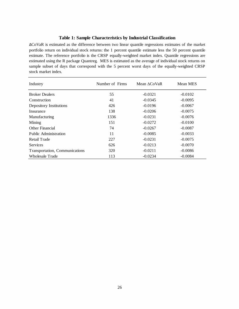
Table 1 describes the sample. It lists the number of firm in the sample by industry and the
average ∆CoVaR and MES estimates for each industry. The ΔCoVaR estimates indicate that, on
average, the construction industry has the largest (negative) ∆CoVaR estimates suggesting that,
on average, this industry has the most systemic risk. Following the construction industry,
according to the ΔCoVaR measure, on average, broker-dealers and mining firms are the next
most important industry sources of systemic risk. According to the MES statistic, on average
broker-dealers are the largest contributors to systemic risk, followed by mining companies and
then the construction industry.
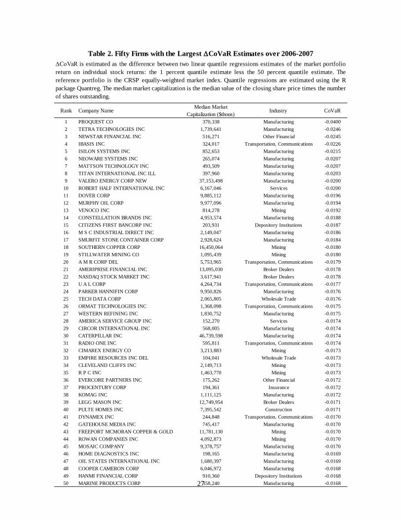
Table 2 lists the fifty companies that exhibit the largest ΔCoVaR measures in descending order
of “systemic risk” importance as indicated by the magnitude of their 1-percent ΔCoVaR
statistics. Most of the firms listed in Table 1 are part of the “real-side” of the economy and have
nothing to do with the financial services sector. Among the firms listed in Table 2 are 7 financial
firms. It is very unlikely that anyone would view any of these 7 firms as “systemically
important.” The depository institution with the largest ΔCoVaR statistic, Citizens First Bancorp,
has less than half the indicated systemic risk of Proquest, the company with the largest ΔCoVaR
systemic risk measure among traded firms.
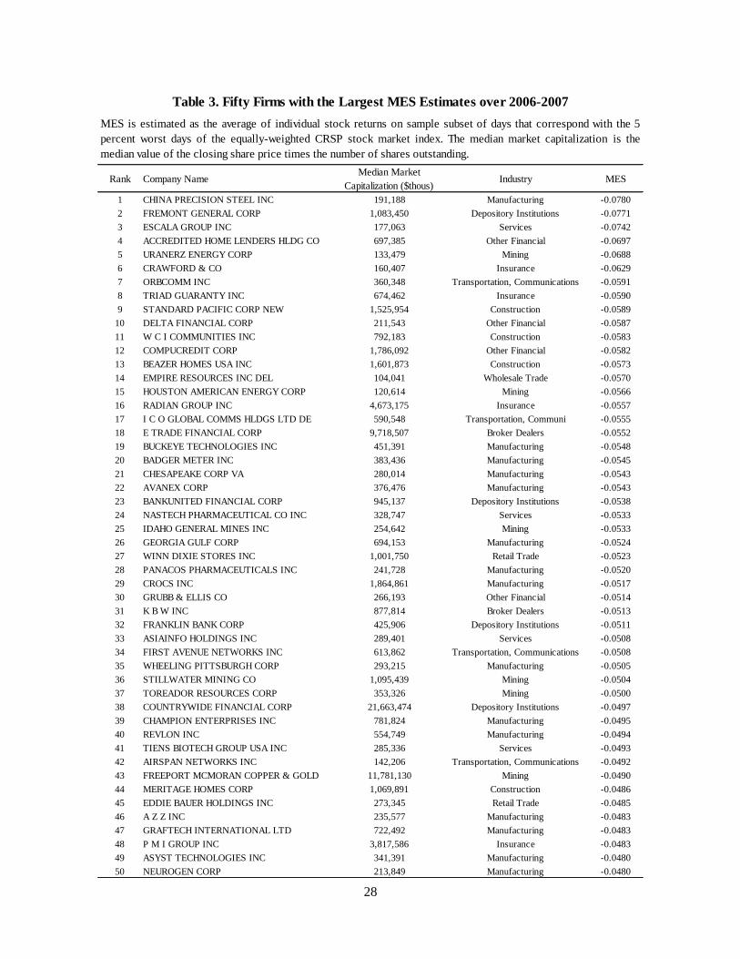
Table 3 lists, in descending order, the fifty companies with the largest (negative) MES systemic
risk measures. While the top-fifty MES firms are still dominated by the real sector, the MES
statistic does generate a list of “high risk” financial firms that did subsequently flounder during
the crisis. CompuCredit, E-trade, Countrywide Financial, IndyMac, BankUnited Financial, Net
8 ∆CoVaR is the difference between the two quantile regression estimates: the 1 percent quantile regression of the
market portfolio on an individual firm’s return less the estimate of the 50 percent quantile regression of the market
return on the individual firm’s return.
9
Bank, Accredited Home Lenders and Fremont General Corporation all experienced serious
distress or failed subsequent to the onset of the financial crisis. Still, none of these firms are
exceptionally large and none was considered to be systemically important or “too-big-to-fail”
during the financial crisis. The firm with the largest MES, China Precision Steel, is not a
financial firm. It is not particularly important for the U.S. domestic economy as more than 60
percent of its operations are in China.
The results in Table 1 through 3 demonstrate that when ΔCoVaR and MES statistics are
calculated for all traded stocks in the years immediately preceding the crisis (2006-2007), the
largest financial institutions that are alleged to be the primary sources of systemic risk for the
economy do not even appear among the list of firms with the fifty most negative ΔCoVaR or
MES estimates. The omission of the largest financial institutions from either list calls into
question previous claims that ΔCoVaR and MES provide accurate measures of a firm’s potential
to cause systemic risk.
Another troubling feature of MES and ΔCoVaR estimates is that there is a systematic
relationship between ΔCoVaR and MES statistics and common market factor beta risk. A
significant share of the cross sectional variation in ΔCoVaR and MES statistics can be attributed
to variation in firms’ systematic risk or the firm’s return correlation with the returns from the
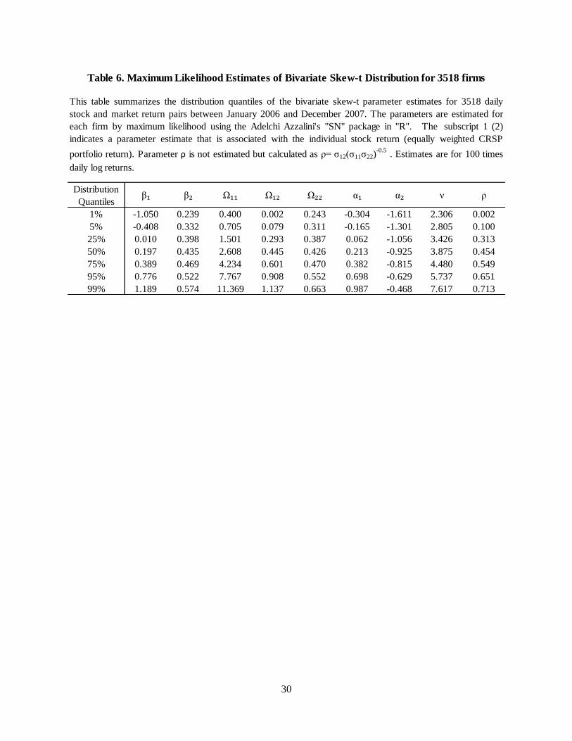
equally-weighted CRSP portfolio.9 Figure 1 shows the fit of a regression of the sample
individual stock MES estimates on their market model beta coefficients estimates. The simple
market model beta coefficient (systematic market risk) explains nearly three-quarters of the
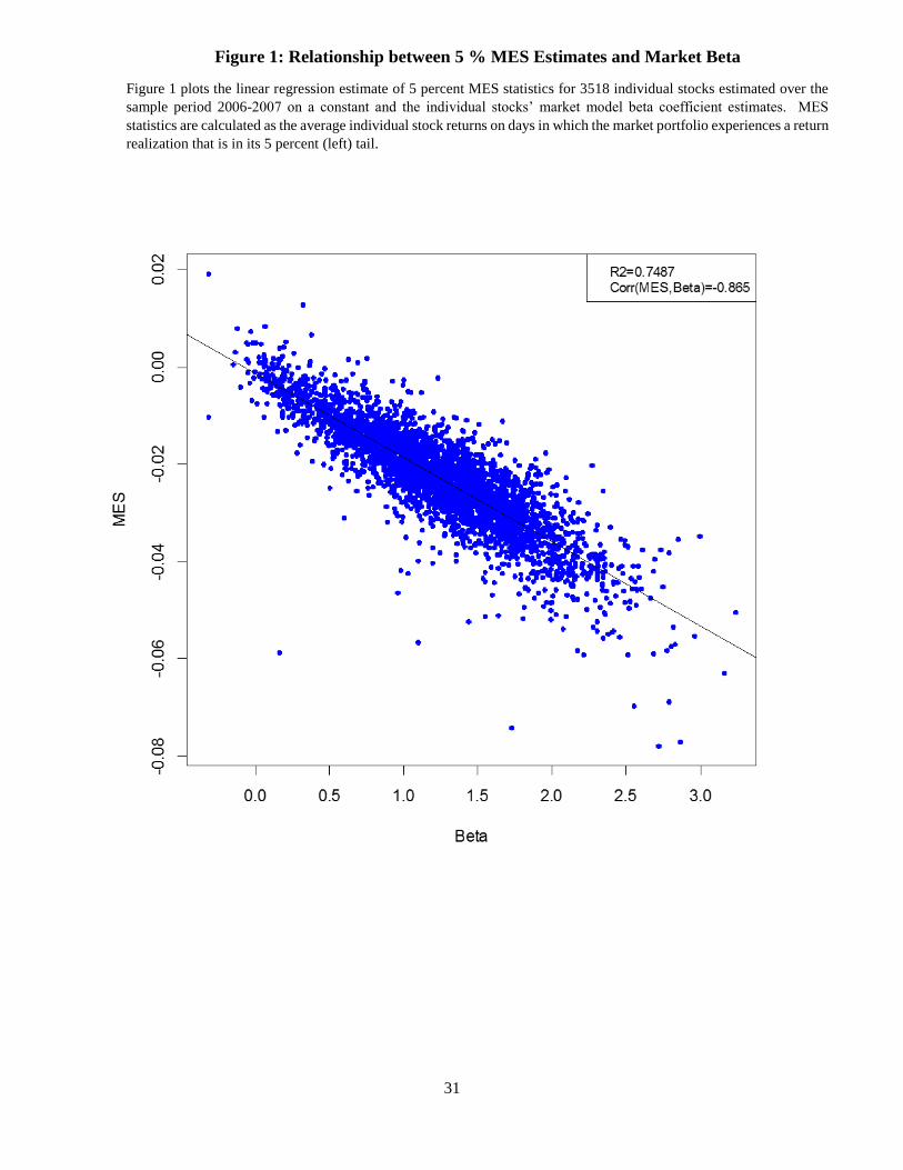
cross-section variation in MES estimates. Figure 2 shows the fit of a cross-sectional regression
of ΔCoVaR estimates on individual stocks’ sample correlation estimates with the equally-
weighted market portfolio return. This regression explains nearly 30 percent of the observed
cross-sectional variation in the sample ΔCoVaR estimates.
The data clearly show that, the greater a firm’s systematic risk, the greater the potential that it
produces a large value ΔCoVaR or MES statistic. Hence, to construct a ΔCoVaR or MES-based
test for systemic risk, it is first necessary to remove the effects of a firm’s systematic risk. In the
next section, we construct ΔCoVaR and MES-based test statistics that remove the effects of
9 Our estimates for ΔCoVaR or MES are similar when we use S&P 500 or value-weighted market portfolio.
10
systematic risk and common factor correlation that are compounded in the “raw” ΔCoVaR and
MES measures.
IV. Systematic Risk Hypothesis Test based on ΔCoVaR and MES Statistics
To construct classical hypothesis tests to detect systemic from ∆CoVaR and MES statistics, we
must adopt a null hypothesis for stock returns that excludes the possibility of systemic risk.
Under the null hypothesis, we develop test statistics using ΔCoVaR and MES estimates that
allow us to assess the probability that the MES and ∆CoVaR estimates would be observed if the
null hypothesis is true. When we observe ∆CoVaR and MES test statistics that are so large that
they are highly unlucky to be generated under the null hypothesis return distribution, we reject
the null hypothesis in favor of alternative stock return generating process that includes the
possibility of systemic risk.
Admissible candidates for the distribution under the null hypothesis must exhibit asymptotic left-
tail independence since we formally define systemic risk as asymptotic dependence in the left tail
of the distribution. The bivariate Gaussian distribution satisfies the independence condition, is
analytically tractable, and given the long history of using the Gaussian distribution to model
stock returns, it is a logical distribution to use initially. In the penultimate section of this paper,
we discuss the performance of our test statistic under alternative hypotheses that deviate from the
Gaussian null hypothesis including alternatives that are asymptotically tail independent and
thereby lack systemic risk.
When (�̃�𝑗, �̃�𝑃) have a bivariate normal distribution, Φ [(𝜇𝑗𝜇𝑃
) , (𝜎𝑗
2 𝜌𝜎𝑗𝜎𝑃
𝜌𝜎𝑗𝜎𝑃 𝜎𝑃2 )], where Φ(𝑎, 𝑏)
represent the Gaussian distribution function with mean “a” and variance “b”. The conditional
distributions are also normal random variables,
�̃�𝑗|(�̃�𝑃 = 𝑟𝑃𝑖) ~ Φ [𝜇𝑗 + 𝜌𝜎𝑗
𝜎𝑃(𝑟𝑃𝑖 − 𝜇𝑃), (1 − 𝜌2)𝜎𝑗
2] (5a)
�̃�𝑃|(�̃�𝑗 = 𝑟𝑗𝑖 )~ Φ [𝜇𝑃 + 𝜌𝜎𝑃
𝜎𝑗(𝑟𝑗𝑖 − 𝜇𝑗), (1 − 𝜌2)𝜎𝑃
2] (5b)
where 𝜇𝑗 and 𝜇𝑃 represent the individual (univariate) return means, 𝜎𝑗2 and 𝜎𝑃
2 represent the
individual return variances and 𝜌 represents the correlation between the returns.
11
Parametric CoVaR for Gaussian Returns
CoVaR can be measured in two ways. One CoVaR measures the conditional VaR of a reference
portfolio conditional on an individual stock experiencing an extreme left-tail return event. A
second possible CoVaR calculation (called the Exposure CoVaR) measures the conditional value
at risk of an individual stock conditional on the reference portfolio experiencing an extreme left-
tail return event. While we derive closed form expressions for both measures, we focus our
analysis on the former measure during the rest of the paper.
First we derive the CoVaR measure for the reference portfolio conditioned on the extreme
negative return of an individual stock. The conditional distribution function for �̃�𝑃 conditional
on �̃�𝑗 equal to its 1 percent value at risk is,
�̃�𝑃| (�̃�𝑗 = Φ−1(. 01, �̃�𝑗)) ~ Φ [𝜇𝑃 + 𝜌𝜎𝑃
𝜎𝑗(Φ−1(. 01, �̃�𝑗) − 𝜇𝑗), (1 − 𝜌2)𝜎𝑃
2] , (6)
and observing Φ−1(. 01, �̃�𝑗) = 𝜇𝑗 − 2.32635 𝜎𝑗, the 1 percent CoVaR for the portfolio
conditional on �̃�𝑗 equal to its 1 percent VaR is,
𝐶𝑜𝑉𝑎𝑅 (�̃�𝑃| (�̃�𝑗 = Φ−1(. 01, �̃�𝑗))) = 𝜇𝑃 − 𝜌𝜎𝑃
𝜎𝑗(2.32635 𝜎𝑗) − 2.32635 𝜎𝑃√1 − 𝜌2 , (7)
The conditional return distribution for the portfolio, conditional on �̃�𝑗 equal to its median is,
�̃�𝑃| (�̃�𝑗 = Φ−1(. 50, �̃�𝑗)) ~ 𝑁[𝜇𝑃, (1 − 𝜌2)𝜎𝑃2]. (8)
Consequently, the CoVaR for the portfolio with �̃�𝑗 evaluated at its median return is,
𝐶𝑜𝑉𝑎𝑅 (�̃�𝑃| (�̃�𝑗 = Φ−1(. 50, �̃�𝑗))) = 𝜇𝑃 − 2.32635𝜎𝑃√1 − 𝜌2 , (9)
Subtracting (8) from (7) and defining 𝛽𝑗𝑃 =𝐶𝑜𝑣(�̃�𝑗,�̃�𝑃)
𝜎𝑃2 , the contribution CoVaR measure is,
∆𝐶𝑜𝑉𝑎𝑅 (�̃�𝑃| (�̃�𝑗 = Φ−1(. 01, �̃�𝑗))) = − 𝛽𝑗𝑃 ∙ 2.32635 𝜎𝑃
2
𝜎𝑗 (10a)
= −𝜌 ∙ 2.32635𝜎𝑃 (10b)
12
Reversing the order of the conditioning variable (i.e., the CoVaR for �̃�𝑗 conditional on �̃�𝑃 equal
to its 1 percent VaR ), it is straight-forward to show that the so-called exposure CoVaR measure
is,
∆𝐶𝑜𝑉𝑎𝑅 (�̃�𝑖| (�̃�𝑃 = Φ−1(. 01, �̃�𝑃))) = − 𝛽𝑗𝑃 ∙ 2.32635 𝜎𝑃, (11a)
= −𝜌 ∙ 2.32635𝜎𝑗 (11b)
Regardless of which return is used to do the conditioning, both ∆CoVaR measures are negatively
related to the correlation between the stock and the reference portfolio return.
1. Parametric MES for Gaussian Returns
The marginal expected shortfall measure is the expected shortfall calculated from a conditional
return distribution. In Acharya, Pedersen, Philippon and Richardson (2010), the conditioning
event is when the return on a reference portfolio, �̃�𝑃, is less than or equal to its 5 percent VaR
value. The reference portfolio could be a well-diversified portfolio representing the entire stock
market, or a portfolio of bank stocks.
Under the assumption of bivariate normality, the conditional stock return is normally distributed,
and consequently,
𝐸(�̃�𝑗|�̃�𝑃 = 𝑟𝑃) = 𝜇𝑗 − 𝜌𝜎𝑗
𝜎𝑃 𝜇𝑃 + 𝜌
𝜎𝑗
𝜎𝑃𝑟𝑃. (12)
Now, if �̃�𝑃 is normally distributed with mean 𝜇𝑃 and standard deviation 𝜎𝑃, then the expected
value of the market return truncated above the value “b” is,
𝐸(�̃�𝑃|�̃�𝑃 < 𝑏) = 𝜇𝑃 − 𝜎𝑃 [𝜙(
𝑏−𝜇𝑃𝜎𝑃
)
Φ(𝑏−𝜇𝑃
𝜎𝑃)], (13)
If b is the lower 5 percent tail value, 𝑏 = 𝜇𝑃 − 1.645𝜎𝑃, and the expected shortfall measure is,
𝐸(�̃�𝑗|�̃�𝑃 < 𝑉𝑎𝑅(�̃�𝑃, 95%)) = 𝜇𝑗 − 𝜌𝜎𝑗 [𝜙(−1.645)
Φ(−1.645)] (14a)
= 𝜇𝑗 − 2.062839 𝜎𝑀 𝛽𝑗𝑃 (14b)
13
where the constant (2.062839) is a consequence of the 5 percent tail conditioning on the market
return, i.e., 𝜙(−1.645)
Φ(−1.645)= 2.062839.
2. Systemic Risk Test Statistics when Returns are Gaussian
Our hypothesis test statistic is constructed as difference between non-parametric and parametric
(Gaussian) ∆CoVaR (or MES) estimates, scaled to remove dependence on a volatility parameter.
Under the null hypothesis of Gaussian returns, the parametric MES and ∆CoVaR estimators are
unbiased and efficient since they are maximum likelihood estimates. Similarly, under the null
hypothesis the alternative non-parametric ∆CoVaR and MES estimators are unbiased, but they
are not efficient as they do not use any information on the parametric form of the stock return
distribution. If the alternative hypothesis is true, nonparametric ∆CoVaR and MES estimators
should have expected values that differ from their parametric Gaussian counterparts. Under the
alternative hypothesis, the magnitude of the nonparametric estimators reflect tail-dependence in
the sample data while their parametric Gaussian estimates do not. Thus, if the alternative
hypothesis that stock returns are in part driven by systemic risk is correct, the nonparametric
estimators should produce larger (more negative) ∆CoVaR and MES statistics.
Under the null hypothesis, the difference between the two estimators (nonparametric and
parametric) has an expected value of 0, but has a sampling error in any given sample. An
important issue is whether the variance of this sampling error is independent of the
characteristics of the stock and portfolio returns that are being analyzed. It turns out that the
difference between the non-parametric and the Gaussian parametric estimators has a sampling
error that depends on both the return correlation and a volatility parameter. We can control for
volatility dependence by normalizing the differences between the nonparametric and parametric
measures by an estimate of the relevant volatility parameter, but we are still left with the returns
correlation as a “nuisance” parameter that must be controlled for when we construct our small
sample Monte Carlo test statistic simulations.
Let ∆𝐶𝑜𝑉𝑎𝑅̌ represent the non-parametric quantile regression estimator for the contribution
∆CoVaR measure. Let ∆𝐶𝑜𝑉𝑎𝑅̂ represent the sample parametric Gaussian estimator for
∆CoVaR, and let 𝜎�̂� represent the sample standard deviation of the returns on the reference
portfolio. We define the CoVaR test statistic as,
14
𝜅𝐶𝑜𝑉𝑎𝑅 = −∆𝐶𝑜𝑉𝑎𝑅̌ −∆𝐶𝑜𝑉𝑎𝑅̂
𝜎�̂�. (15)
Under the Gaussian null hypothesis, it can be easily demonstrated the sampling distribution of
𝜅𝐶𝑜𝑉𝑎𝑅 depends only on the correlation parameter between the stock returns and the returns on
the reference portfolio.
Under the alternative hypothesis of systemic risk, ∆𝐶𝑜𝑉𝑎𝑅 −̌ ∆𝐶𝑜𝑉𝑎𝑅̂ is expected to be
negative, and since �̂�𝑃 is positive, systemic risk is evident when the test statistic produces a large
positive value. Statistical significance is determined by comparing the test value for 𝜅𝐶𝑜𝑉𝑎𝑅 with
its sampling distribution under the null. When the test value of 𝜅𝐶𝑜𝑉𝑎𝑅 is in the far right-hand
tail of its sampling distribution, we can reject the null hypothesis of no systemic risk. The critical
value used to establish statistical significance determines the type 1 error rate for the test. For
example, rejecting the null hypothesis for test values at or above the 95 percent quantile of the
sampling distribution for 𝜅𝐶𝑜𝑉𝑎𝑅 is consistent with a 5 percent type 1 error meaning there is at
most 5 percent chance of rejecting a true null hypothesis.
Let 𝑀𝐸�̌� represent the non-parametric estimator for MES. The literature defines it as the average
individual stock return on days when the reference portfolio has a return realization in its lower
tail. We condition on reference portfolio returns in the 5 percent tail. Let 𝑀𝐸�̂� represent the
sample parametric Gaussian estimator for MES and �̂�𝑖 represent the sample standard deviation of
the individual stock return in the calculation. We define the MES test statistic as,
𝜅𝑀𝐸𝑆 = −𝑀𝐸�̌�−𝑀𝐸�̂�
�̂�𝑖 (17)
Under the alternative hypothesis of systemic risk, 𝑀𝐸�̌� is expected to produce a larger negative
number compared to 𝑀𝐸�̂�, and since �̂�𝑖 is positive, systemic risk is evident when the test statistic
produces a large positive value. As in the ∆CoVaR case, this test statistic still depends on the
correlation between the stock and the reference portfolio, so correlation is a “nuisance”
parameter that enters into the sampling distribution critical value calculations.
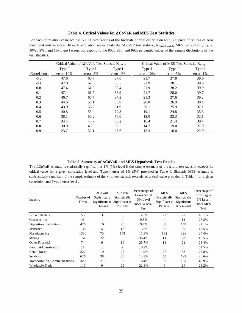
In Table 4 we report the small sample distribution 1, 5 and 10 percent critical value estimates for
the 𝜅𝐶𝑜𝑉𝑎𝑅 and 𝜅𝑀𝐸𝑆 for 12 different portfolio-stock return correlation assumptions between -0.2
15
and 0.9.10 The critical values are calculated using Monte Carlo Simulation11 for a sample size of
500 observations, the equivalent of about two years of daily data. We focus on a two-year
estimation window because the characteristics of institutions, especially large financial
institutions, change very quickly over time through mergers and acquisitions. The critical value
statistics we report are based on 50,000 Monte Carlo simulations.
V. Systemic Risk Test Application to 2006-2007 Stock Returns Data
1. Estimation Methodology
We use daily CRSP stock return data from the period 2006-2007 to calculate 𝜅𝐶𝑜𝑉𝑎𝑅 and 𝜅𝑀𝐸𝑆.
The data set construction is discussed in Section III.
Nonparametric CoVaR
We estimate the nonparametric ΔCoVaR statistic, ∆𝐶𝑜𝑉𝑎𝑅̌ , in three steps:
We run a 1-percent quantile regression of the CRSP equally weighted market return, 𝑅𝑀
on 𝑅𝑗 and estimate 𝛽�̂�, the stock return coefficient in the quantile regression.
Estimate the 1-percent sample quantile and the median of the firm’s stock return, 𝑅𝑗,
𝑉𝑎�̌�(𝑅𝑗, 𝑞) and 𝑉𝑎�̌�(𝑅𝑗, 0.50).
Nonparametric ΔCoVaR estimator is defined as:
∆𝐶𝑜𝑉𝑎𝑅̌ (𝑅𝑀 |𝑅𝑗 = 𝑉𝑎𝑅(𝑅𝑗 , 𝑞)) = 𝛽�̂� (𝑉𝑎�̌�(𝑅𝑗 , 𝑞) − 𝑉𝑎�̌�(𝑅𝑗, 0.50)) (18)
We estimate our parametric ΔCoVaR statistic, ∆𝐶𝑜𝑉𝑎𝑅̂ , using equation (11) and the
sample moments of individual stock returns and the equally-weighted market portfolio
returns.
10Under the null hypothesis, we use Monte Carlo simulations to construct the sampling distribution for the
hypothesis test statistics. The 90th, 95th, and 99th percentiles of the estimated sampling distribution determine,
respectively, the 10 percent, 5 percent and 1 percent critical values of the test statistic. If the null hypothesis true,
and we reject the null hypothesis if the sample statistic exceeds the critical threshold value, the type I error is 10
percent, 5 percent or 1 percent respectively because there is less than a 10 percent, 5 percent or 1 percent probability
of observing a larger value than the threshold in any random sample of 500 observations if the null hypothesis is
true. 11 We use the quantile regression package QUANTREG in R written by Roger Koenker.
16
Nonparametric MES
We estimate nonparametric MES, 𝑀𝐸𝑆,̌ as the average of individual stock returns on sample
subset of days that correspond with the 5 percent worst days of the equally-weighted broad stock
market index.
𝑀𝐸�̌�(𝑅𝑗 , 5%) =∑ 𝑅𝑗 𝐼(𝑅𝑚<𝑉𝑎𝑅(𝑅𝑚,5%))
∑ 𝐼(𝑅𝑚<𝑉𝑎𝑅(𝑅𝑚,5%))=
1
𝑁∑ 𝑅𝑗𝑅𝑚<𝑉𝑎𝑅5%
(19)
where I(.) is the indicator function and N is the number of 5 percent worst days for the market.
We measure parametric MES, 𝑀𝐸�̂�, using expression (14) and sample moments for individual
stock returns and the returns on the equally-weighted market portfolio.
2. Hypothesis Test Results
Table 5 summarizes 𝜅𝐶𝑜𝑉𝑎𝑅 and 𝜅𝑀𝐸𝑆 hypothesis test results. Evaluated at the 5 percent level of
the test, the 𝜅𝐶𝑜𝑉𝑎𝑅 test identifies 496 of 3518 firms as systemically important, or 14 percent of
all sample firms. Ranked by industry, the mining industry has the largest share of firms
identified as systemically important (36.4 percent), followed by “other financial” (25.7 percent)
and wholesale trade (22.1 percent). Among the remaining financial services industries, broker
dealers have the largest share of firms identified as systemically important (14.5 percent),
followed by insurance (13 percent) and depository institutions (9.4 percent).
The 𝜅𝑀𝐸𝑆 test identifies a much larger number of firms as systemically important. At the 5
percent level, the MES test identifies 979 firms as potential sources of systemic risk, or 28
percent of the firms in the sample. Among specific industries, public administration has the
largest share of firms with systemic risk potential (54.5 percent), followed by broker dealers
(49.1 percent), and transportation, communications and utilities (46.9 percent). Among the
remaining financial services industries, insurance had the largest share of firms identified as
systemically risky (43.5 percent), followed by depository institutions (37.7 percent) and other
financial (28.4 percent).
These formal hypothesis tests identify many more firms as sources of systemic compared to
previous papers that examined only a small subset of financial institutions. And, unlike prior
papers, because we examine all firms with actively traded equity, we identify many real-side
17
firms as systemically important. If systemic risk is manifest as asymptotic tail dependence in
stock returns, and if our MES and CoVaR tests reliably identify tail dependence, then a lot firms
will require systemic risk taxes or heightened prudential standards as prophylactic measures to
keep the financial system safe. Clearly, the issue of the reliability of our test statistics is central.
The Gaussian null hypothesis is very restrictive and it is important to understand whether
commonly observed non-Gaussian stock return characteristics can lead to a test rejection even
when stock returns are asymptotically tail independent.
VI. Do 𝜿𝑪𝒐𝑽𝒂𝑹 and 𝜿𝑴𝑬𝑺 Rejections Detect Asymptotic Tail Dependence?
Let (𝑅1̃, 𝑅2̃) represent a bivariate random vector with individual univariate marginal distributions
defined by 𝐹1(𝑟) = 𝑃𝑟(�̃�1 ≤ 𝑟), and 𝐹2(𝑟) = 𝑃𝑟(�̃�2 ≤ 𝑟). Let 𝐿(𝑢) represent the conditional
probability,
𝐿(𝑢) = 𝑃𝑟(𝐹1(𝑅1) < 𝑢| 𝐹2(𝑅2) < 𝑢) (20)
The asymptotic left tail dependence between 𝑅1̃ and 𝑅2̃ is defined as, 𝐿 = lim𝑢→0
𝐿(𝑢). If this limit
is 0, the random variables are asymptotically independent in their left tails. If the limit is
positive, then the random variables have asymptotic tail dependence in the left tail. The larger is
the value of the limit, the stronger is the left-tail dependence.
Many distributions can be used to model stock returns, and among these, any distribution that
exhibits asymptotic left-tail independence is a candidate for use as the null hypothesis in the
construction of our CoVaR and MES test statistics. In this section, we consider the properties of
the Gaussian null hypothesis against a family of alternative distributions nested within the
bivariate skew-t distribution. Depending on parameter values, the bivariate skew-t-distribution
nests the bivariate skewed Gaussian distribution and the bivariate symmetric student-t and
Gaussian distributions.
Let 𝑑 be the dimension of the multivariate distribution. Let 𝑦 be a (𝑑 × 1) random vector,
and 𝛽 and 𝛼 (𝑑 × 1) vectors of constants. Ω is a (𝑑 × 𝑑) positive definite matrix. 𝜈 ∈
(0, ∞) is the scalar that represents the degrees of freedom parameter. The multivariate skew-t
density 𝑦~𝑓𝑇(𝑦, 𝛽, Ω, 𝛼, 𝜈) is defined in Azzalini (2005):
18
𝑓𝑇(𝑦, 𝛽, Ω, 𝛼, 𝜈) = 2𝑡𝑑(𝑦; 𝛽, 𝛺, 𝜈)𝑇1 (𝛼𝑇𝜔−1(𝑦 − 𝛽) (𝜈+𝑑
𝑄𝑦+𝜈)
0.5
; 𝜈 + 𝑑) (21)
where, 𝑡𝑑(𝑦; 𝛽, 𝛺, 𝜈) =𝛤(0.5(𝜈+𝑑))
|𝛺|0.5(𝜋𝜈)𝑑 2⁄ 𝛤(0.5𝜈)(1+𝑄𝑦 𝜈⁄ )(𝜈+𝑑) 2⁄
is the density function of a d-dimensional student t variate with ν degrees of freedom, and
T1(x;ν+d) denotes the scalar t distribution with ν+d degrees of freedom. 𝛽 is the location
parameter which controls the distribution means, 𝛼 is the parameter which controls the skewness
of the distribution,12 and Ω is a generalized covariance matrix.13 The remaining parameters are,
𝜔 = 𝑑𝑖𝑎𝑔(𝛺)0.5 and 𝑄𝑦 = (𝑦 − 𝛽)𝑇𝛺−1(𝑦 − 𝛽).
The skew-t distribution nests the symmetric t-distribution, (𝛼 = 0 ,0 < 𝜈 < ∞), the skewed
Gaussian distribution, (𝛼 ≠ 0, 𝜈 = ∞), and the symmetric Gaussian distribution, (𝛼 = 0, 𝜈 = ∞).
The flexibility of the skew-t distribution facilities the process of evaluating the behavior of the
∆CoVaR and MES hypothesis test statistics under a number of plausible alternative hypothesis.
It is well-known that the Gaussian distribution is asymptotically tail independent. The skewed-
Gaussian distribution is also asymptotically tail independent [Bortot (2010)]. Both the skewed
and symmetric t-distributions have asymptotic tail dependence where the tail dependence
depends on the degrees of freedom parameter, the generalized correlation parameter, and the
skewness parameters.
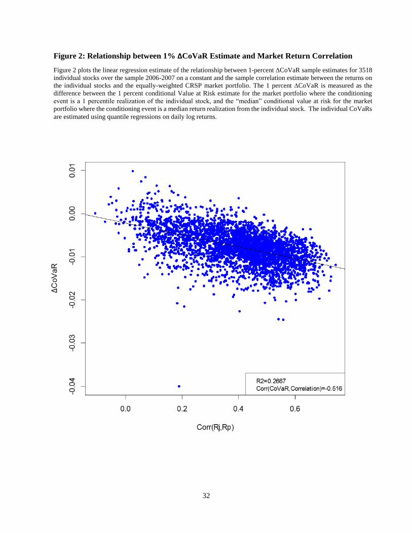
The expression for the asymptotic left tail dependence of a bivariate symmetric t distribution is
given by,
𝐿𝑠𝑦𝑚 𝑡 = 2𝑇1 (−√(𝜈+1)(1−𝜌)
√1+𝜌, 𝜐 + 1) (22)
where 𝑇1(𝑥, 𝜈) is the distribution function for a univariate t distribution with 𝜈 degrees of
freedom. Figure 3 illustrates the relationship between the asymptotic tail dependence in the
symmetric bivariate t distribution and the distribution’s correlation and degrees of freedom
12 α is not equal to but monotonically related to skewness. α=0 implies a symmetric non-skewed distribution,
whereas α > 0 (α < 0) implies positive (negative) skewness. It is also called the “shape” or the “slant” parameter. 13 Ω is equal to the covariance matrix of y only when the skewness and kurtosis are 0 (α=0, ν=∞).
19
parameters. The higher the bivariate correlation and smaller the degrees of freedom, the stronger
the distribution’s asymptotic tail dependence.
In most cases, there is no closed-form expression for the asymptotic tail dependence of a
bivariate skew-t distribution. In the special case where the skew is identical across the individual
random variables, 𝛼1 = 𝛼2 = 𝛼 , the distribution’s asymptotic tail dependence is given by
𝐿𝑠𝑘𝑒𝑤−𝑡 = 𝐾(𝛼, 𝜈, 𝜌) 2𝑇1 (−√(𝜈+1)(1−𝜌)
√1+𝜌, 𝜐 + 1), (23)
where, 𝐾(𝛼, 𝜈, 𝜌) =𝑇1(2𝛼√
(𝜈+2)(1+𝜌)
2;𝜈+2)
𝑇1(𝛼(1+𝜌)√𝜈+1
√1+𝛼2(1−𝜌2)
; 𝜈+1)
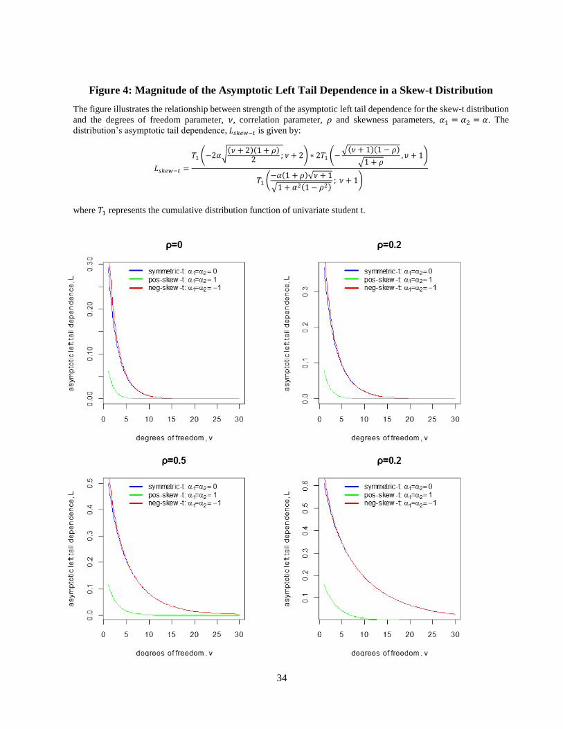
Figure 4 illustrates the relationship between strength of the asymptotic tail dependence for the
skew-t distribution and the degrees of freedom parameter, 𝜈, correlation parameter ρ, and
skewness parameters 𝛼1 = 𝛼2 = 𝛼. We observe that negative skewness increases tail
dependence, but only when the degree of freedom is low, that is when tails of the distribution are
fat.
We estimated the parameters for the bivariate skew-t distribution using maximum likelihood for
each of the 3518 stocks in our sample paired with the CRSP equally-weighted market return.14
The subscript 1 (2) indicates a parameter estimate that is associated with the individual stock
return (equally-weighted CRSP portfolio return). The distribution of resulting parameter
estimates is reported in Table 6. Key parameters of interest in Table 6 are 𝛼1, 𝛼2, 𝜐, and 𝜌.
Table 6 shows that, for most of the stocks in the sample over the 2006-2007 sample period, �̂�1 >
0, indicating that most individual stock’s return distributions are positively skewed. This finding
is consistent with the literature [e.g., Singleton and Wingender (2006), or Carr et al, (2002)].
𝛼2 is the parameter that determines the skewness of the market return distribution. While its
magnitude varies among the 3518 bivariate maximum likelihood estimations, in all cases, �̂�2 <
0, indicating that the market return distribution is negatively skewed.15 Again, a negatively
14 We used the “sn” package in “R” written by Adelchi Azzalini 15 The market skewness parameter is estimated simultaneously with the individual stock’s skewness parameter and
the single degrees of freedom parameter for the bivariate distribution. Ideally we would prefer to estimate the entire
20
skewed market return distribution is consistent with the literature [e.g., Fama (1965), Duffee
(1995), Carr et al, (2002)), or Adrian and Rosenberg (2008)].
The degrees of freedom parameter, 𝜐, is the most important determinant of the asymptotic tail
dependence of the bivariate distribution. The results in Table 6 show that in more than 75
percent of the sample, 𝜐 < 4.5.
Our test statistics are derived under the null hypothesis that stock returns are bivariate normal.
The results in Table 6 suggest that the Gaussian null hypothesis is incorrect in a large number of
cases as indicated by non-zero skewness parameter estimates and a predominance of small
values for the degrees of freedom estimate. It is important to understand how alternative return
distributions affect the sampling distribution of our test statistics. For example, will return
distributions with asymptotic tail dependence reliably cause our test statistic to reject the
Gaussian null? Will any degree of asymptotic tail dependence cause a rejection of the null
hypothesis or must the asymptotic tail dependence reach a critical strength before it is detected?
Will skewness trigger a rejection of null hypothesis even when returns have no asymptotic tail
dependence? The bivariate skew-t distribution provides an ideal model of stock returns that can
be used to investigate all of these questions.
In the remainder of this section we generate simulated stock return data from alternative
parameterizations of the skew-t distributions and estimate the sampling distribution for our
hypothesis test statistics using Monte Carlo simulation and kernel density estimation. For
alternative parameterizations, we calculate our hypothesis test statistics for 10,000 samples of
500 observations. We consider alternative parameterizations of the skew-t distribution that use
parameter values that more realistically represent the underlying distribution of the actual stock
return series.
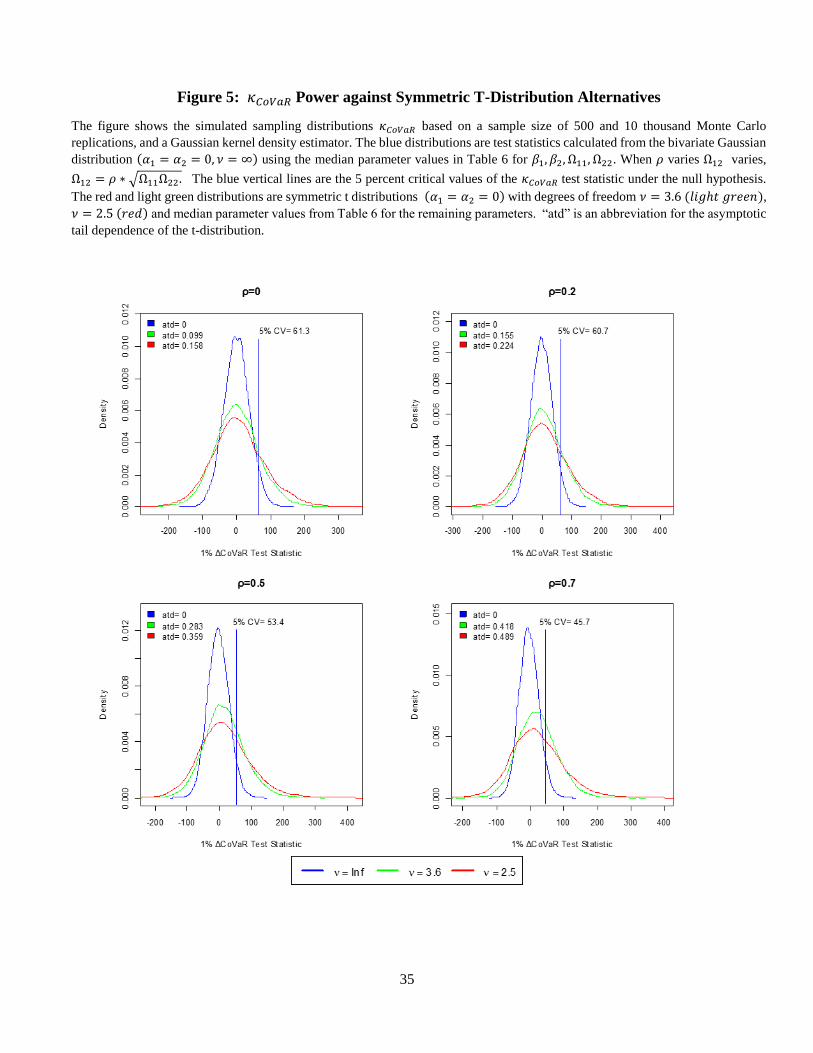
We first investigate whether 𝜅𝐶𝑜𝑉𝑎𝑅 and 𝜅𝑀𝐸𝑆 have statistical power against alternative
hypothesis that include negative asymptotic tail dependence. Figure 5 plots the sampling
distribution for the 𝜅𝐶𝑜𝑉𝑎𝑅 test statistic under the Gaussian null hypothesis distribution and two
multivariate (3518 dimensions) skew-t distribution simultaneously and thereby get one set of parameters for the
market portfolio. However, with only 500 daily observations, the joint return system not be identified unless
additional structural simplification are imposed to reduce the number of independent parameters that must be
estimated.
21
symmetric t distributions with degrees of freedom that are characteristic of the estimates
produced in our cross section of stock returns.
Recall that the asymptotic tail dependence of the t distribution is largest when the correlation is
strong and the degrees of freedom parameter is small. Across the panels in Figure 5, as 𝜌
increases, we plot the sampling distributions for 𝜅𝐶𝑜𝑉𝑎𝑅 test statistics as the underlying
distributions have stronger and stronger asymptotic tail dependence. For most of the
distributions, the sampling distribution for 𝜅𝐶𝑜𝑉𝑎𝑅 under the null hypothesis substantially
overlaps the sampling distributions for 𝜅𝐶𝑜𝑉𝑎𝑅 under the alternative hypothesis, and the
alternative hypothesis sampling distributions have relatively little cumulative probability to the
right of the 5 percent critical value under the null hypothesis. This relationship indicates that is
highly probable that, should the alternative hypothesis be true, the calculated test statistics may
not reject the null. In other words, the 𝜅𝐶𝑜𝑉𝑎𝑅 test has lower power for detecting asymptotic tail
dependence. This is especially true for 𝜌 = 0 and 𝜌 = .2 panels when the asymptotic tail
dependence of the alternative t distributions is under 30 percent.
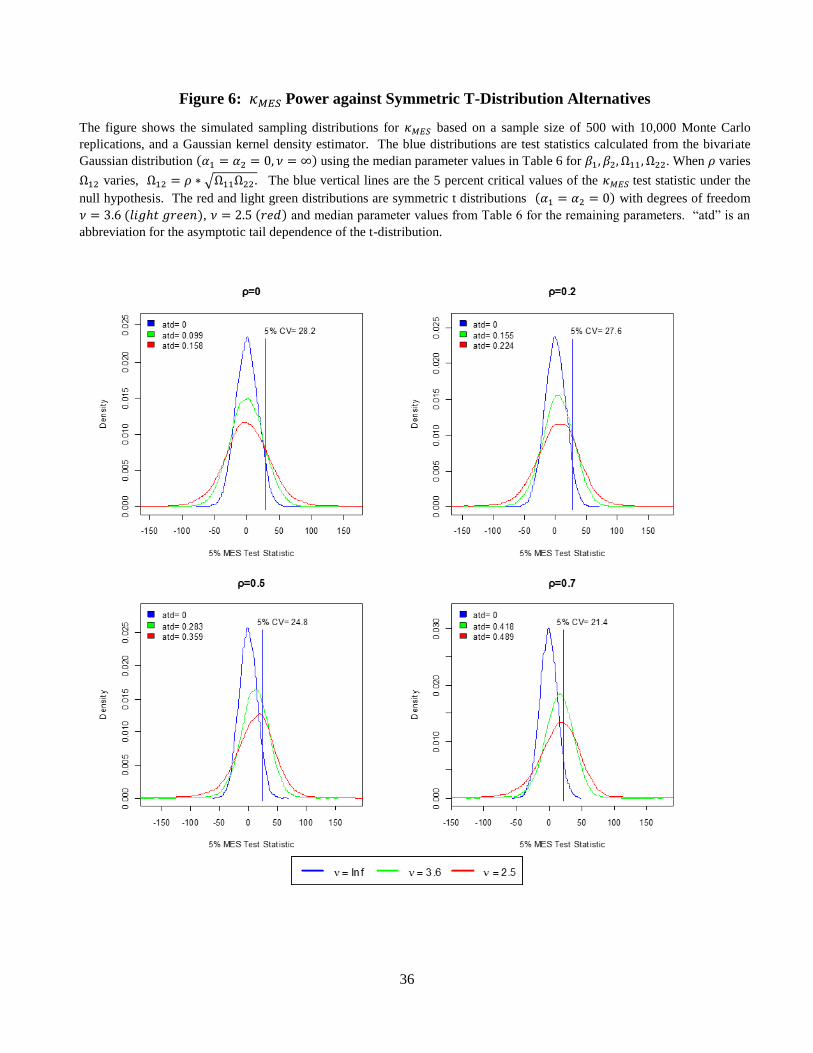
Figure 6 repeats the symmetric t distribution power simulations for the 𝜅𝑀𝐸𝑆 test statistic and the
results are similar to those for the 𝜅𝐶𝑜𝑉𝑎𝑅 statistic. While the 𝜅𝑀𝐸𝑆 test has slightly better power
characteristics compared to 𝜅𝐶𝑜𝑉𝑎𝑅, it still has poor power unless the returns have very strong
asymptotic tail dependence. For example, the 𝜌=.7 panel shows that, even when asymptotic tail
dependence is 0.489, the power of the 𝜅𝑀𝐸𝑆 test is still only about 50 percent meaning that if the
alternative hypothesis of tail dependence is true, the test will not reject the null hypothesis about
half the time.
What is more, the figures also show that as, asymptotic tail dependency increases, the variance of
𝜅𝐶𝑜𝑉𝑎𝑅 and 𝜅𝑀𝐸𝑆 test statistics grow significantly. Hence, almost paradoxically, these test
statistics become noisier and less efficient when the distribution has greater systemic risk. This
tradeoff between the magnitude of systemic risk to be detected and the efficiency of the tests
statistic estimators may be small sample issue. Relatively short time series (about 500 daily
observations) are too small to effectively detect tail dependence. However, the use of longer time
series is impractical because the characteristics of the individual firms, especially the largest
financial institutions, can change dramatically within a period of only a few years.
22
Taken together Figures 5 and 6 make a strong case against using ∆CoVaR and MES as measures
of systemic risk. Even after correcting for market risk, and developing a formal hypothesis test,
the ∆CoVaR and MES are not going to be able to accurately distinguish returns with asymptotic
tail dependence from returns that are independent in the asymptotic tails. While the lack of
statistical power calls into question the value of further research on refining our ∆CoVaR and
MES hypothesis test statistics, it is still valuable to better understand the consequences of
adopting the Gaussian null hypothesis.
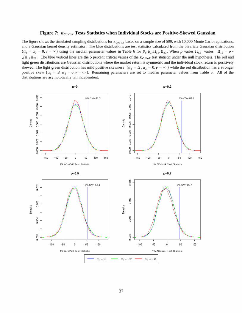
Figures 7 and 8 analyze the behavior of the 𝜅𝐶𝑜𝑉𝑎𝑅 and 𝜅𝑀𝐸𝑆 test statistics under alternative
return distributions in which market returns are symmetric Gaussian, but individual firm returns
are positively skewed Gaussian. Under these alternative distributions, returns are asymptotically
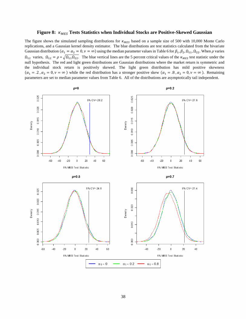
independent and the null hypothesis should not be rejected. Figures 7 and 8 show that the
sampling distributions for 𝜅𝐶𝑜𝑉𝑎𝑅 and 𝜅𝑀𝐸𝑆 test statistics under the alternative hypothesis are
very similar to the sampling distribution under the null, and there is little risk that positively
skewed Gaussian individual returns (with symmetric Gaussian market returns) will generate
many false rejections of the null.
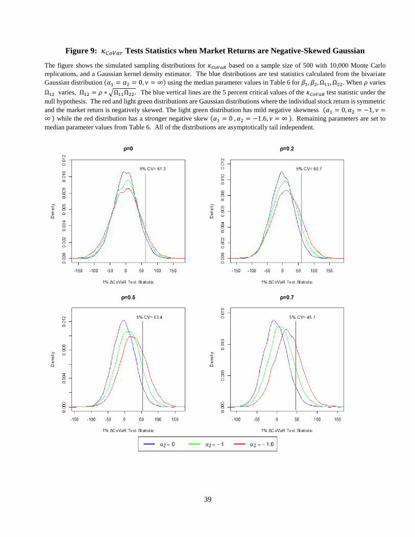
Figures 9 and 10 analyze the behavior of the 𝜅𝐶𝑜𝑉𝑎𝑅 and 𝜅𝑀𝐸𝑆 test statistics under alternative
return distributions in which market returns are negatively skewed Gaussian, but individual firm
returns are symmetric Gaussian. Returns are asymptotically independent and the null hypothesis
should not be rejected. Figures 9 and 10 clearly show that negatively skewed market returns can
cause false rejection of the null hypothesis. This is especially true when the individual stocks and
the market are highly positively correlated. The 𝜅𝐶𝑜𝑉𝑎𝑅 seems to be more susceptible to this
type of error, but for both statistics, the Gaussian null hypothesis critical values will cause false
rejections that could be misinterpreted as evidence of tail dependence and systemic risk.
Figures 11 and 12 analyze the behavior of the 𝜅𝐶𝑜𝑉𝑎𝑅 and 𝜅𝑀𝐸𝑆 test statistics under alternative
return distributions in which market returns are negatively skewed Gaussian, and individual firm
returns are positively-skewed Gaussian. Negative market skewness with positive individual
stock skewness is the most prevalent pattern observed in the data. Here again, returns are
asymptotically independent and the null hypothesis should not be rejected. The pattern in
Figures 11 and 12 is similar. Mild positive individual stock skewness with relatively strong
negative market skewness and strong positive return correlation is a pattern that is likely to
23
generate false rejections of the null hypothesis. This particular skewness and correlation pattern
is predominant in the 2006-2007 sample data suggesting that the large number of rejections in
our sample may owe in part to an overly restrictive null hypothesis. Generalizing the test
statistic to incorporate a skewed Gaussian distribution under the null would be a step in the right
direction, but again the poor ∆CoVaR and MES power characteristics show there will be limited
benefits for further refinements.
VII. Summary and Conclusions
In this paper, we develop a new methodology to control for systematic risk biases inherent in
CoVaR and MES risk measures and construct classical hypothesis tests for the presence of
systemic risk. The methodology and test statistics are based on the Gaussian model of stock
returns. We use Monte Carlo simulation to estimate the critical values of the sampling
distributions of our proposed test statistics and use these critical values to test for evidence of
systemic risk in a wide cross section of stocks using daily return data over the period 2006-2007.
Our methodology introduces formal hypothesis tests to detect systemic risk, tests which
heretofore have been absent from the literature. However, our hypothesis tests are composite
tests, and as a consequence they do not provide an ideal solution to the CoVaR and MES
measurement issues we identify. Our hypothesis tests for MES and ∆CoVaR require a
maintained hypothesis of a specific return distribution under the null hypothesis. The composite
nature of the null hypothesis is problematic because it can lead to false indications of systemic
risk. For example, we show that, depending on the return generating process, our tests reject
may the null hypothesis of no systemic risk even when returns are generated by a tail-
independent distributions. Thus, the choice of a specific return distribution to characterize returns
under the null hypothesis is a crucial aspect of systemic risk test design that has garnered little
attention in the literature. While this finding suggests a research agenda focused on clarifying
the nature of stock returns under null hypothesis, our findings on the power of ∆CoVaR and
MES tests suggest that these efforts would be wasted.
In particular, our simulation results suggest that ∆CoVaR and MES statistics are unlikely to
detect asymptotic tail dependence unless the tail dependence is very strong. And even in cases
with strong tail dependence, the power of these tests is limited. The power limitations are a
consequence of sampling variance of ∆CoVaR and MES statistics. In small samples (e.g. 500
24
observations), as tail dependence strengthens, the variance of the MES and CoVaR estimators
increases. If systemic risk is truly manifest as asymptotic left-tail dependence in stock returns,
∆CoVaR and MES seem incapable of providing a reliable measure of a firm’s systemic risk
potential.
References
Acharya, V., Engle, R., Richardson, M., 2012. “Capital Shortfall: A New Approach to Ranking
and Regulating Systemic Risks”, The American Economic Review 102, 59-64.
Acharya, V. V., Pedersen, L., Philippon, T., and Richardson, M., 2010. “Measuring Systemic
Risk”, Technical report, Department of Finance, Working paper, NYU Stern School of Business.
Adrian, T. and Brunnermeier, M. K., 2011. “CoVaR”, FRB of New York. Staff Report No. 348.
Adrian, Tobias, and Joshua Rosenberg, 2008. “Stock Returns and Volatility: Pricing the Short-
Run and Long-Run Components of Market Risk, Journal of Finance, Vol. 63, No. 6, pp. 2997-
3030.
Azzalini, A., (2005). Skew-normal distribution and related multivariate families. Scandinavian
Journal of Statistics, Vol 32, pp. 159-188.
Azzalini, A. and A. Capitanio, (2003). Distributions generated by perturbation of symmetry with
emphasis on a multivariate skew t distribution. Journal of the Royal Statistical Society, B, Vol
65, pp. 367-389.
Benoit, S. G. Colletaz, C. Hurlin, and C. Perignon, 2012. “A Theoretical and Empirical
Comparison of Systemic Risk Measures.” Working Paper, University of Orleans, France.
Bisias, D., Flood, M., Lo, A., and Valavanis, S., 2012. A survey of systemic risk analytics. U.S.
Department of Treasury, Office of Financial Research Working Paper.
Bortot, Paola, 2010, Tail dependence in bivariate skew-Normal and skew-t distributions.
Department of Statistical Sciences, Working paper, University of Bologna
Brownlees, C. and Engle, R., 2012. “Volatility, Correlation and Tails for Systemic Risk
Measurement”, Working Paper, New York University.
Carr, P., H. Geman, D. B. Madan, and M. Yor, (2002). The fine structure of asset returns: An
empirical investigation. The Journal of Business, 75(2), 305-333.
25
Duffee, G. R., 1995. “Stock Returns and Volatility: A Firm-Level Analysis. Journal of Financial
Economics, Vol. 37, pp. 399-420.
Fama, E. F., 1965. “The Behavior of Stock Market Prices,” Journal of Business, Vol. 38, pp. 34-
105.
Kupiec, Paul, 2012. “Discussion of Acharya, V.; Engle, R.; Richardson, M., ‘Capital Shortfall: A
New Approach to Ranking and Regulating Systemic Risks,’ American Economic Association
Meetings, Chicago, Ill., January 2012.
Kupiec, Paul, 1998. “Stress Testing in a Value at Risk Framework,” The Journal of Derivatives,
Vol. 6, No. 1.
Singleton, Clay, and J. Wingender, 1986. “Skewness Persistence in Common Stock Returns,”
The Journal of Financial and Quantitative Analysis, Vol. 21, No. 3, pp. 335-341.
26
Industry Number of Firms Mean DCoVaR Mean MES
Broker Dealers 55 -0.0321 -0.0102
Construction 41 -0.0345 -0.0095
Depository Institutions 426 -0.0196 -0.0067
Insurance 138 -0.0206 -0.0075
Manufacturing 1336 -0.0231 -0.0076
Mining 151 -0.0272 -0.0100
Other Financial 74 -0.0267 -0.0087
Public Administration 11 -0.0085 -0.0033
Retail Trade 227 -0.0231 -0.0075
Services 626 -0.0213 -0.0070
Transportation, Communications 320 -0.0211 -0.0086
Wholesale Trade 113 -0.0234 -0.0084
Table 1: Sample Characteristics by Industrial Classification
∆CoVaR is estimated as the difference between two linear quantile regressions estimates of the market
portfolio return on individual stock returns: the 1 percent quantile estimate less the 50 percent quantile
estimate. The reference portfolio is the CRSP equally-weighted market index. Quantile regressions are
estimated using the R package Quantreg. MES is estimated as the average of individual stock returns on
sample subset of days that correspond with the 5 percent worst days of the equally-weighted CRSP
stock market index.
27
Rank Company NameMedian Market
Capitalization ($thous)Industry CoVaR
1 PROQUEST CO 370,338 Manufacturing -0.0400
2 TETRA TECHNOLOGIES INC 1,739,641 Manufacturing -0.0246
3 NEWSTAR FINANCIAL INC 516,271 Other Financial -0.0245
4 IBASIS INC 324,017 Transportation, Communications -0.0226
5 ISILON SYSTEMS INC 852,653 Manufacturing -0.0215
6 NEOWARE SYSTEMS INC 265,074 Manufacturing -0.0207
7 MATTSON TECHNOLOGY INC 493,509 Manufacturing -0.0207
8 TITAN INTERNATIONAL INC ILL 397,960 Manufacturing -0.0203
9 VALERO ENERGY CORP NEW 37,153,498 Manufacturing -0.0200
10 ROBERT HALF INTERNATIONAL INC 6,167,046 Services -0.0200
11 DOVER CORP 9,885,112 Manufacturing -0.0196
12 MURPHY OIL CORP 9,977,096 Manufacturing -0.0194
13 VENOCO INC 814,278 Mining -0.0192
14 CONSTELLATION BRANDS INC 4,953,574 Manufacturing -0.0188
15 CITIZENS FIRST BANCORP INC 203,931 Depository Institutions -0.0187
16 M S C INDUSTRIAL DIRECT INC 2,149,047 Manufacturing -0.0186
17 SMURFIT STONE CONTAINER CORP 2,928,624 Manufacturing -0.0184
18 SOUTHERN COPPER CORP 16,450,064 Mining -0.0180
19 STILLWATER MINING CO 1,095,439 Mining -0.0180
20 A M R CORP DEL 5,753,965 Transportation, Communications -0.0179
21 AMERIPRISE FINANCIAL INC 13,095,030 Broker Dealers -0.0178
22 NASDAQ STOCK MARKET INC 3,617,941 Broker Dealers -0.0178
23 U A L CORP 4,264,734 Transportation, Communications -0.0177
24 PARKER HANNIFIN CORP 9,950,826 Manufacturing -0.0176
25 TECH DATA CORP 2,065,805 Wholesale Trade -0.0176
26 ORMAT TECHNOLOGIES INC 1,368,098 Transportation, Communications -0.0175
27 WESTERN REFINING INC 1,830,752 Manufacturing -0.0175
28 AMERICA SERVICE GROUP INC 152,270 Services -0.0174
29 CIRCOR INTERNATIONAL INC 568,005 Manufacturing -0.0174
30 CATERPILLAR INC 46,739,598 Manufacturing -0.0174
31 RADIO ONE INC 595,811 Transportation, Communications -0.0174
32 CIMAREX ENERGY CO 3,213,883 Mining -0.0173
33 EMPIRE RESOURCES INC DEL 104,041 Wholesale Trade -0.0173
34 CLEVELAND CLIFFS INC 2,149,713 Mining -0.0173
35 R P C INC 1,463,770 Mining -0.0173
36 EVERCORE PARTNERS INC 175,262 Other Financial -0.0172
37 PROCENTURY CORP 194,361 Insurance -0.0172
38 KOMAG INC 1,111,125 Manufacturing -0.0172
39 LEGG MASON INC 12,749,954 Broker Dealers -0.0171
40 PULTE HOMES INC 7,395,542 Construction -0.0171
41 DYNAMEX INC 244,848 Transportation, Communications -0.0170
42 GATEHOUSE MEDIA INC 745,417 Manufacturing -0.0170
43 FREEPORT MCMORAN COPPER & GOLD 11,781,130 Mining -0.0170
44 ROWAN COMPANIES INC 4,092,873 Mining -0.0170
45 MOSAIC COMPANY 9,378,757 Manufacturing -0.0170
46 HOME DIAGNOSTICS INC 198,165 Manufacturing -0.0169
47 OIL STATES INTERNATIONAL INC 1,680,397 Manufacturing -0.0169
48 COOPER CAMERON CORP 6,046,972 Manufacturing -0.0168
49 HANMI FINANCIAL CORP 910,360 Depository Institutions -0.0168
50 MARINE PRODUCTS CORP 358,240 Manufacturing -0.0168
Table 2. Fifty Firms with the Largest DCoVaR Estimates over 2006-2007
∆CoVaR is estimated as the difference between two linear quantile regressions estimates of the market portfolio
return on individual stock returns: the 1 percent quantile estimate less the 50 percent quantile estimate. The
reference portfolio is the CRSP equally-weighted market index. Quantile regressions are estimated using the R
package Quantreg. The median market capitalization is the median value of the closing share price times the number
of shares outstanding.
28
Rank Company NameMedian Market
Capitalization ($thous)Industry MES
1 CHINA PRECISION STEEL INC 191,188 Manufacturing -0.0780
2 FREMONT GENERAL CORP 1,083,450 Depository Institutions -0.0771
3 ESCALA GROUP INC 177,063 Services -0.0742
4 ACCREDITED HOME LENDERS HLDG CO 697,385 Other Financial -0.0697
5 URANERZ ENERGY CORP 133,479 Mining -0.0688
6 CRAWFORD & CO 160,407 Insurance -0.0629
7 ORBCOMM INC 360,348 Transportation, Communications -0.0591
8 TRIAD GUARANTY INC 674,462 Insurance -0.0590
9 STANDARD PACIFIC CORP NEW 1,525,954 Construction -0.0589
10 DELTA FINANCIAL CORP 211,543 Other Financial -0.0587
11 W C I COMMUNITIES INC 792,183 Construction -0.0583
12 COMPUCREDIT CORP 1,786,092 Other Financial -0.0582
13 BEAZER HOMES USA INC 1,601,873 Construction -0.0573
14 EMPIRE RESOURCES INC DEL 104,041 Wholesale Trade -0.0570
15 HOUSTON AMERICAN ENERGY CORP 120,614 Mining -0.0566
16 RADIAN GROUP INC 4,673,175 Insurance -0.0557
17 I C O GLOBAL COMMS HLDGS LTD DE 590,548 Transportation, Communi -0.0555
18 E TRADE FINANCIAL CORP 9,718,507 Broker Dealers -0.0552
19 BUCKEYE TECHNOLOGIES INC 451,391 Manufacturing -0.0548
20 BADGER METER INC 383,436 Manufacturing -0.0545
21 CHESAPEAKE CORP VA 280,014 Manufacturing -0.0543
22 AVANEX CORP 376,476 Manufacturing -0.0543
23 BANKUNITED FINANCIAL CORP 945,137 Depository Institutions -0.0538
24 NASTECH PHARMACEUTICAL CO INC 328,747 Services -0.0533
25 IDAHO GENERAL MINES INC 254,642 Mining -0.0533
26 GEORGIA GULF CORP 694,153 Manufacturing -0.0524
27 WINN DIXIE STORES INC 1,001,750 Retail Trade -0.0523
28 PANACOS PHARMACEUTICALS INC 241,728 Manufacturing -0.0520
29 CROCS INC 1,864,861 Manufacturing -0.0517
30 GRUBB & ELLIS CO 266,193 Other Financial -0.0514
31 K B W INC 877,814 Broker Dealers -0.0513
32 FRANKLIN BANK CORP 425,906 Depository Institutions -0.0511
33 ASIAINFO HOLDINGS INC 289,401 Services -0.0508
34 FIRST AVENUE NETWORKS INC 613,862 Transportation, Communications -0.0508
35 WHEELING PITTSBURGH CORP 293,215 Manufacturing -0.0505
36 STILLWATER MINING CO 1,095,439 Mining -0.0504
37 TOREADOR RESOURCES CORP 353,326 Mining -0.0500
38 COUNTRYWIDE FINANCIAL CORP 21,663,474 Depository Institutions -0.0497
39 CHAMPION ENTERPRISES INC 781,824 Manufacturing -0.0495
40 REVLON INC 554,749 Manufacturing -0.0494
41 TIENS BIOTECH GROUP USA INC 285,336 Services -0.0493
42 AIRSPAN NETWORKS INC 142,206 Transportation, Communications -0.0492
43 FREEPORT MCMORAN COPPER & GOLD 11,781,130 Mining -0.0490
44 MERITAGE HOMES CORP 1,069,891 Construction -0.0486
45 EDDIE BAUER HOLDINGS INC 273,345 Retail Trade -0.0485
46 A Z Z INC 235,577 Manufacturing -0.0483
47 GRAFTECH INTERNATIONAL LTD 722,492 Manufacturing -0.0483
48 P M I GROUP INC 3,817,586 Insurance -0.0483
49 ASYST TECHNOLOGIES INC 341,391 Manufacturing -0.0480
50 NEUROGEN CORP 213,849 Manufacturing -0.0480
Table 3. Fifty Firms with the Largest MES Estimates over 2006-2007
MES is estimated as the average of individual stock returns on sample subset of days that correspond with the 5
percent worst days of the equally-weighted CRSP stock market index. The median market capitalization is the
median value of the closing share price times the number of shares outstanding.
29
Type I Type I Type I Type I Type I Type I
Correlation error=10% error=5% error=1% error=10% error=5% error=1%
-0.2 47.6 60.7 87.0 21.7 27.8 39.6
-0.1 47.8 62.3 88.5 21.9 28.1 39.8
0.0 47.4 61.3 88.4 21.9 28.2 39.9
0.1 47.1 61.5 88.9 21.7 28.0 39.7
0.2 46.7 60.7 87.2 21.3 27.6 39.2
0.3 44.6 58.1 83.8 20.8 26.9 38.4
0.4 43.0 56.2 81.9 20.1 25.9 37.1
0.5 40.8 53.4 79.8 19.1 24.8 35.3
0.6 38.1 50.2 74.0 18.0 23.3 33.1
0.7 34.4 45.7 68.2 16.4 21.4 30.4
0.8 30.0 40.3 59.5 14.7 19.0 27.0
0.9 23.7 32.1 48.6 12.3 16.0 22.9
Critical Value of DCoVaR Test Statistic KCoVaR Critical Value of MES Test Statistic, KMES
For each correlation value we run 50,000 simulations of the bivariate normal distribution with 500 pairs of returns of zero
mean and unit variance. In each simulation we estimate the DCoVaR test statistic, KCoVaR and the MES test statistic, KMES.
10% , 5% , and 1% Type I errors correspond to the 90th, 95th and 99th percentile values of the sample distibutions of the
test statistics.
Table 4. Critical Values for DCoVaR and MES Test Statistics
IndustryNumber of
Firms
DCoVaR
Statistically
Significant at
1% level
DCoVaR
Statistically
Significant at
5% level
Percentage of
Firms Sig. at
5% Level
under DCoVaR
Test
MES
Statistically
Significant at
1% level
MES
Statistically
Significant
at 5% level
Percentage of
Firms Sig. at
5% Level
under MES
Test
Broker Dealers 55 3 8 14.5% 22 27 49.1%
Construction 41 1 4 9.8% 4 11 26.8%
Depository Institutions 426 16 40 9.4% 88 158 37.1%
Insurance 138 5 18 13.0% 36 60 43.5%
Manufacturing 1336 75 159 11.9% 132 326 24.4%
Mining 151 22 55 36.4% 11 28 18.5%
Other Financial 74 9 19 25.7% 13 21 28.4%
Public Administration 11 1 2 18.2% 0 6 54.5%
Retail Trade 227 10 27 11.9% 27 63 27.8%
Services 626 38 80 12.8% 50 129 20.6%
Transportation, Communications 320 21 59 18.4% 80 150 46.9%
Wholesale Trade 113 9 25 22.1% 8 24 21.2%
Table 5. Summary of DCoVaR and MES Hypothesis Test Results
The DCoVaR estimate is statistically significant at 1% (5%) level if the sample estimate of the κCoVaR test statistic exceeds its
critical value for a given correlation level and Type I error of 1% (5%) provided in Table 4. Similarly MES estimate is
statististically significant if the sample estimate of the κMES test statistic exceeds its critical value provided in Table 4 for a given
correlation and Type I error level .
30
Distribution
Quantilesβ₁ β₂ Ω₁₁ Ω₁₂ Ω₂₂ α₁ α₂ ν ρ
1% -1.050 0.239 0.400 0.002 0.243 -0.304 -1.611 2.306 0.002
5% -0.408 0.332 0.705 0.079 0.311 -0.165 -1.301 2.805 0.100
25% 0.010 0.398 1.501 0.293 0.387 0.062 -1.056 3.426 0.313
50% 0.197 0.435 2.608 0.445 0.426 0.213 -0.925 3.875 0.454
75% 0.389 0.469 4.234 0.601 0.470 0.382 -0.815 4.480 0.549
95% 0.776 0.522 7.767 0.908 0.552 0.698 -0.629 5.737 0.651
99% 1.189 0.574 11.369 1.137 0.663 0.987 -0.468 7.617 0.713
This table summarizes the distribution quantiles of the bivariate skew-t parameter estimates for 3518 daily
stock and market return pairs between January 2006 and December 2007. The parameters are estimated for
each firm by maximum likelihood using the Adelchi Azzalini's "SN" package in "R". The subscript 1 (2)
indicates a parameter estimate that is associated with the individual stock return (equally weighted CRSP
portfolio return). Parameter ρ is not estimated but calculated as ρ= σ12(σ11σ22)-0.5
. Estimates are for 100 times
daily log returns.
Table 6. Maximum Likelihood Estimates of Bivariate Skew-t Distribution for 3518 firms
31
Figure 1: Relationship between 5 % MES Estimates and Market Beta
Figure 1 plots the linear regression estimate of 5 percent MES statistics for 3518 individual stocks estimated over the
sample period 2006-2007 on a constant and the individual stocks’ market model beta coefficient estimates. MES
statistics are calculated as the average individual stock returns on days in which the market portfolio experiences a return
realization that is in its 5 percent (left) tail.
32
Figure 2: Relationship between 1% ΔCoVaR Estimate and Market Return Correlation
Figure 2 plots the linear regression estimate of the relationship between 1-percent ∆CoVaR sample estimates for 3518
individual stocks over the sample 2006-2007 on a constant and the sample correlation estimate between the returns on
the individual stocks and the equally-weighted CRSP market portfolio. The 1 percent ∆CoVaR is measured as the
difference between the 1 percent conditional Value at Risk estimate for the market portfolio where the conditioning
event is a 1 percentile realization of the individual stock, and the “median” conditional value at risk for the market
portfolio where the conditioning event is a median return realization from the individual stock. The individual CoVaRs
are estimated using quantile regressions on daily log returns.
33
Figure 3: Symmetric T-Distribution Asymptotic Tail Dependence as a Function of
Correlation and Degrees of Freedom
The figure plots the asymptotic tail dependence for various levels of degrees of freedom and correlation for the
symmetric bivariate t distribution. Asymptotic tail dependence is given by:
𝐿𝑠𝑦𝑚 𝑡 = 2𝑇1 (−√(𝜈 + 1)(1 − 𝜌)
√1 + 𝜌, 𝜐 + 1)
34
Figure 4: Magnitude of the Asymptotic Left Tail Dependence in a Skew-t Distribution
The figure illustrates the relationship between strength of the asymptotic left tail dependence for the skew-t distribution
and the degrees of freedom parameter, 𝜈, correlation parameter, 𝜌 and skewness parameters, 𝛼1 = 𝛼2 = 𝛼. The
distribution’s asymptotic tail dependence, 𝐿𝑠𝑘𝑒𝑤−𝑡 is given by:
𝐿𝑠𝑘𝑒𝑤−𝑡 =
𝑇1 (−2𝛼√(𝜈 + 2)(1 + 𝜌)2
; 𝜈 + 2) ∗ 2𝑇1 (−√(𝜈 + 1)(1 − 𝜌)
√1 + 𝜌, 𝜐 + 1)
𝑇1 (−𝛼(1 + 𝜌)√𝜈 + 1
√1 + 𝛼2(1 − 𝜌2); 𝜈 + 1)
where 𝑇1 represents the cumulative distribution function of univariate student t.
35
Figure 5: 𝜅𝐶𝑜𝑉𝑎𝑅 Power against Symmetric T-Distribution Alternatives
The figure shows the simulated sampling distributions 𝜅𝐶𝑜𝑉𝑎𝑅 based on a sample size of 500 and 10 thousand Monte Carlo
replications, and a Gaussian kernel density estimator. The blue distributions are test statistics calculated from the bivariate Gaussian
distribution (𝛼1 = 𝛼2 = 0, 𝜈 = ∞) using the median parameter values in Table 6 for 𝛽1, 𝛽2, Ω11, Ω22. When 𝜌 varies Ω12 varies,
Ω12 = 𝜌 ∗ √Ω11Ω22. The blue vertical lines are the 5 percent critical values of the 𝜅𝐶𝑜𝑉𝑎𝑅 test statistic under the null hypothesis.
The red and light green distributions are symmetric t distributions (𝛼1 = 𝛼2 = 0) with degrees of freedom 𝜈 = 3.6 (𝑙𝑖𝑔ℎ𝑡 𝑔𝑟𝑒𝑒𝑛),
𝜈 = 2.5 (𝑟𝑒𝑑) and median parameter values from Table 6 for the remaining parameters. “atd” is an abbreviation for the asymptotic
tail dependence of the t-distribution.
36
Figure 6: 𝜅𝑀𝐸𝑆 Power against Symmetric T-Distribution Alternatives
The figure shows the simulated sampling distributions for 𝜅𝑀𝐸𝑆 based on a sample size of 500 with 10,000 Monte Carlo
replications, and a Gaussian kernel density estimator. The blue distributions are test statistics calculated from the bivariate
Gaussian distribution (𝛼1 = 𝛼2 = 0, 𝜈 = ∞) using the median parameter values in Table 6 for 𝛽1, 𝛽2, Ω11, Ω22. When 𝜌 varies
Ω12 varies, Ω12 = 𝜌 ∗ √Ω11Ω22. The blue vertical lines are the 5 percent critical values of the 𝜅𝑀𝐸𝑆 test statistic under the
null hypothesis. The red and light green distributions are symmetric t distributions (𝛼1 = 𝛼2 = 0) with degrees of freedom
𝜈 = 3.6 (𝑙𝑖𝑔ℎ𝑡 𝑔𝑟𝑒𝑒𝑛), 𝜈 = 2.5 (𝑟𝑒𝑑) and median parameter values from Table 6 for the remaining parameters. “atd” is an
abbreviation for the asymptotic tail dependence of the t-distribution.
37
Figure 7: 𝜅𝐶𝑜𝑉𝑎𝑟 Tests Statistics when Individual Stocks are Positive-Skewed Gaussian
The figure shows the simulated sampling distributions for 𝜅𝐶𝑜𝑉𝑎𝑅 based on a sample size of 500, with 10,000 Monte Carlo replications,
and a Gaussian kernel density estimator. The blue distributions are test statistics calculated from the bivariate Gaussian distribution
(𝛼1 = 𝛼2 = 0, 𝜈 = ∞) using the median parameter values in Table 6 for 𝛽1, 𝛽2, Ω11, Ω22. When 𝜌 varies Ω12 varies, Ω12 = 𝜌 ∗
√Ω11Ω22. The blue vertical lines are the 5 percent critical values of the 𝜅𝐶𝑜𝑉𝑎𝑅 test statistic under the null hypothesis. The red and
light green distributions are Gaussian distributions where the market return is symmetric and the individual stock return is positively
skewed. The light green distribution has mild positive skewness (𝛼1 = .2 , 𝛼2 = 0, 𝜈 = ∞ ) while the red distribution has a stronger
positive skew (𝛼1 = .8 , 𝛼2 = 0, 𝜈 = ∞ ). Remaining parameters are set to median parameter values from Table 6. All of the
distributions are asymptotically tail independent.
38
Figure 8: 𝜅𝑀𝐸𝑆 Tests Statistics when Individual Stocks are Positive-Skewed Gaussian
The figure shows the simulated sampling distributions for 𝜅𝑀𝐸𝑆 based on a sample size of 500 with 10,000 Monte Carlo
replications, and a Gaussian kernel density estimator. The blue distributions are test statistics calculated from the bivariate
Gaussian distribution (𝛼1 = 𝛼2 = 0, 𝜈 = ∞) using the median parameter values in Table 6 for 𝛽1, 𝛽2, Ω11, Ω22. When 𝜌 varies
Ω12 varies, Ω12 = 𝜌 ∗ √Ω11Ω22. The blue vertical lines are the 5 percent critical values of the 𝜅𝑀𝐸𝑆 test statistic under the
null hypothesis. The red and light green distributions are Gaussian distributions where the market return is symmetric and
the individual stock return is positively skewed. The light green distribution has mild positive skewness
(𝛼1 = .2 , 𝛼2 = 0, 𝜈 = ∞ ) while the red distribution has a stronger positive skew (𝛼1 = .8 , 𝛼2 = 0, 𝜈 = ∞ ). Remaining
parameters are set to median parameter values from Table 6. All of the distributions are asymptotically tail independent.
39
Figure 9: 𝜅𝐶𝑜𝑉𝑎𝑟 Tests Statistics when Market Returns are Negative-Skewed Gaussian
The figure shows the simulated sampling distributions for 𝜅𝐶𝑜𝑉𝑎𝑅 based on a sample size of 500 with 10,000 Monte Carlo
replications, and a Gaussian kernel density estimator. The blue distributions are test statistics calculated from the bivariate
Gaussian distribution (𝛼1 = 𝛼2 = 0, 𝜈 = ∞) using the median parameter values in Table 6 for 𝛽1, 𝛽2, Ω11, Ω22. When 𝜌 varies
Ω12 varies, Ω12 = 𝜌 ∗ √Ω11Ω22. The blue vertical lines are the 5 percent critical values of the 𝜅𝐶𝑜𝑉𝑎𝑅 test statistic under the
null hypothesis. The red and light green distributions are Gaussian distributions where the individual stock return is symmetric
and the market return is negatively skewed. The light green distribution has mild negative skewness (𝛼1 = 0, 𝛼2 = −1, 𝜈 =
∞ ) while the red distribution has a stronger negative skew (𝛼1 = 0 , 𝛼2 = −1.6, 𝜈 = ∞ ). Remaining parameters are set to
median parameter values from Table 6. All of the distributions are asymptotically tail independent.
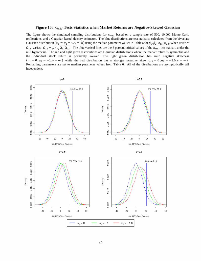
40
Figure 10: 𝜅𝑀𝐸𝑆 Tests Statistics when Market Returns are Negative-Skewed Gaussian
The figure shows the simulated sampling distributions for 𝜅𝑀𝐸𝑆 based on a sample size of 500, 10,000 Monte Carlo
replications, and a Gaussian kernel density estimator. The blue distributions are test statistics calculated from the bivariate
Gaussian distribution (𝛼1 = 𝛼2 = 0, 𝜈 = ∞) using the median parameter values in Table 6 for 𝛽1, 𝛽2, Ω11, Ω22. When 𝜌 varies
Ω12 varies, Ω12 = 𝜌 ∗ √Ω11Ω22. The blue vertical lines are the 5 percent critical values of the 𝜅𝑀𝐸𝑆 test statistic under the
null hypothesis. The red and light green distributions are Gaussian distributions where the market return is symmetric and
the individual stock return is positively skewed. The light green distribution has mild negative skewness
(𝛼1 = 0 , 𝛼2 = −1, 𝜈 = ∞ ) while the red distribution has a stronger negative skew (𝛼1 = 0 , 𝛼2 = −1.6, 𝜈 = ∞ ).
Remaining parameters are set to median parameter values from Table 6. All of the distributions are asymptotically tail
independent.
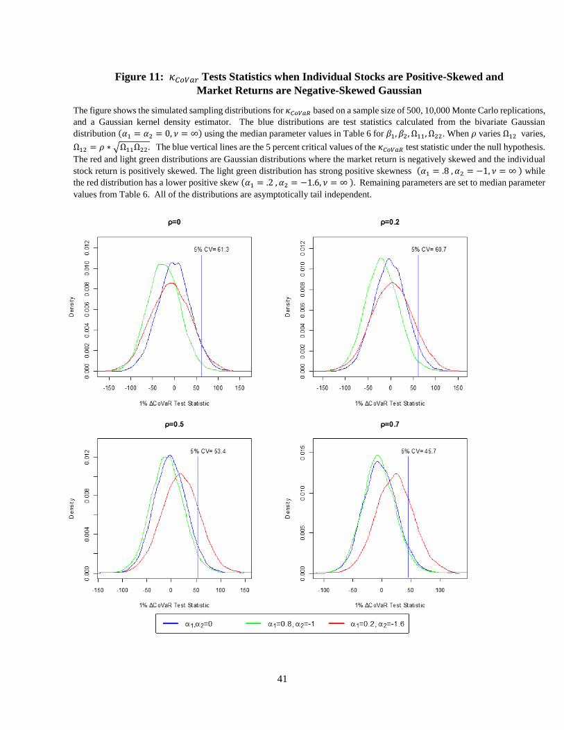
41
Figure 11: 𝜅𝐶𝑜𝑉𝑎𝑟 Tests Statistics when Individual Stocks are Positive-Skewed and
Market Returns are Negative-Skewed Gaussian
The figure shows the simulated sampling distributions for 𝜅𝐶𝑜𝑉𝑎𝑅 based on a sample size of 500, 10,000 Monte Carlo replications,
and a Gaussian kernel density estimator. The blue distributions are test statistics calculated from the bivariate Gaussian
distribution (𝛼1 = 𝛼2 = 0, 𝜈 = ∞) using the median parameter values in Table 6 for 𝛽1, 𝛽2, Ω11, Ω22. When 𝜌 varies Ω12 varies,
Ω12 = 𝜌 ∗ √Ω11Ω22. The blue vertical lines are the 5 percent critical values of the 𝜅𝐶𝑜𝑉𝑎𝑅 test statistic under the null hypothesis.
The red and light green distributions are Gaussian distributions where the market return is negatively skewed and the individual
stock return is positively skewed. The light green distribution has strong positive skewness (𝛼1 = .8 , 𝛼2 = −1, 𝜈 = ∞ ) while
the red distribution has a lower positive skew (𝛼1 = .2 , 𝛼2 = −1.6, 𝜈 = ∞ ). Remaining parameters are set to median parameter
values from Table 6. All of the distributions are asymptotically tail independent.
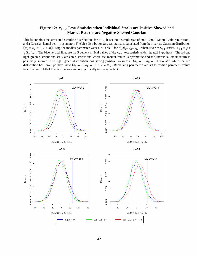
42
Figure 12: 𝜅𝑀𝐸𝑆 Tests Statistics when Individual Stocks are Positive-Skewed and
Market Returns are Negative-Skewed Gaussian
This figure plots the simulated sampling distributions for 𝜅𝑀𝐸𝑆 based on a sample size of 500, 10,000 Monte Carlo replications,
and a Gaussian kernel density estimator. The blue distributions are test statistics calculated from the bivariate Gaussian distribution
(𝛼1 = 𝛼2 = 0, 𝜈 = ∞) using the median parameter values in Table 6 for 𝛽1, 𝛽2, Ω11, Ω22. When 𝜌 varies Ω12 varies, Ω12 = 𝜌 ∗
√Ω11Ω22. The blue vertical lines are the 5 percent critical values of the 𝜅𝑀𝐸𝑆 test statistic under the null hypothesis. The red and
light green distributions are Gaussian distributions where the market return is symmetric and the individual stock return is
positively skewed. The light green distribution has strong positive skewness (𝛼1 = .8 , 𝛼2 = −1, 𝜈 = ∞ ) while the red
distribution has lower positive skew (𝛼1 = .2 , 𝛼2 = −1.6, 𝜈 = ∞ ). Remaining parameters are set to median parameter values
from Table 6. All of the distributions are asymptotically tail independent.