taking the plunge: an introduction to undertaking seascape

Taking the Plunge: An Introduction to Undertaking Seascape Genetic Studies and Using Biophysical Models

Libby Liggins1,*, Eric A. Treml1,2 and Cynthia Riginos11School of Biological Sciences, The University of Queensland 2Department of Zoology, The University of Melbourne* Correspondence address: L. Liggins, School of Biological Sciences, The University of Queensland, St. Lucia Qld 4072, Australia. E-mail: [email protected].

AbstractThe field of seascape genetics aims to evaluate the effects of environmental features on spatial genetic patterns of marine organisms. Although many methods of genetic analysis and inference appropriate to ‘‘marine landscapes’’ derive from terrestrial landscape genetics, aspects of marine living introduce special challenges for assessing spatial genetic variation. For instance, marine organisms are often highly dispersive, so that genetic patterns can be subtle, and the temporal variability of the marine environment makes these patterns difficult to characterise. Tools and techniques from oceanography can help describe the highly connected and dynamic nature of the marine environment. In particular, models incorporating physical oceanography and species attributes in realistic simulations (e.g. biophysical models) can help us understand this complex process and formulate spatially explicit biologically-informed predictions of gene flow. Thus, researchers embarking on a seascape genetic study need a solid understanding of marine organisms and spatial genetics perhaps combined with knowledge of physical oceanography and ecological modeling. Although some researchers may acquire proficiency in all of these areas, seascape genetic studies incorporating biophysical modeling are likely to bring together groups of investigators with complementary expertise. This preliminary guide is intended to be a starting point for a reader new to either seascape genetics or biophysical models.

What’s in a Bit of Water?

Seascape genetics is a sub discipline of ‘‘landscape genetics’’ focused on marine habitats and species. Landscape genetics draws upon methods from landscape ecology and geography to characterize spatial factors and uses methods derived from population genetics as metrics of genetic variation (Manel et al. 2003; Storfer et al. 2010). The majority of landscape genetic studies to date have been in terrestrial habitats (Storfer et al. 2010), but there has been increasing interest in applying these concepts to marine organisms and seascapes. Examples of seascape genetic studies include those interested in the historical colonisation and migration patterns among marine populations, contemporary patterns of dispersal among populations, and patterns of neutral and adaptive genetic variation in relation to past or present features of the seascape (see Riginos & Liggins 2013, this issue, for a review of studies). Here, we focus on the methodologies that apply to such investigations.

The most challenging element of the marine environment for traditional spatial genetic techniques is ocean dynamics (Galindo et al. 2006; Selkoe et al. 2008). The fluidity of the ocean and the strength of ocean currents can lead populations to be highly connected by dispersive individuals, and disconnected by ocean barriers, in non-intuitive ways. In addition, the physical template of the ocean, including salinity, light, temperature and currents, fluctuates through time (see Figure 1, Riginos & Liggins 2013). Furthermore, life histories of marine organisms often differ from terrestrial organisms (Strathmann 1990) and can vary substantially among marine organisms, so that inter-population genetic exchange can occur via gametes, embryos, larvae and⁄or adults, in any combination. These various modes of exchange are differentially impacted by ocean dynamics; for example, ocean currents are a dispersal vector for some passive species (and in some locations and seasons only) and for other life history strategies (e.g. strong-swimming or benthic) a current may be either irrelevant or act as a barrier.

Many seascape genetic studies have benefited from considering their genetic data alongside physical oceanographic models (e.g. White et al. 2010; Alberto et al. 2011; similar to the utility of wind models in the study of gene flow via wind-dispersed pollen or seeds in land plants, see Levin et al. 2003). However, certain life history features and behaviors of marine organisms are also important

Geography Compass 7/3 (2013): 173–196, 10.1111/gec3.12031

Liggins et al. 2013 - Seascape genetic methods including biophysical models

determinants of dispersal (Gerlach et al. 2007; Kingsford et al. 2002; Strathmann 1990) prompting the use of biologically-informed models similar to those used for terrestrial animals and already used for some marine mammals (e.g. Austin et al. 2004). Thus, coupled biological-physical models (hereafter biophysical models) incorporating ocean circulation data have emerged as away to help generate seascape genetic hypotheses, produce biophysical data to correlate with genetic data, and examine the mechanisms underlying genetic patterns.

This preliminary guide is intended to supplement the accompanying review (‘Seascape genetics: populations, individuals, and genes marooned and adrift’, Riginos & Liggins 2013, current issue) in which distinguishing features of the marine environment are described, and influential seascape genetic studies are discussed. In the present paper, we focus on experimental design and methodologies: we first identify considerations specific to seascape genetics in the context of present-day methods and analytical developments in the field of landscape genetics. In the second part of this paper, we introduce biophysical models, review their use in combination with genetic data, and highlight relevant technical considerations in their use. (Note that important terms are explained in the appended glossary).

Undertaking Seascape Genetic Studies

The central purpose of seascape genetic studies is to infer associations between spatial environmental features and genetic variation that may be neutral (shaped by processes of mutation, genetic drift and gene flow) or adaptive (influenced by natural selection). Although the focal environmental features may differ from those of terrestrial landscape studies, many methods of analysis and inference will be the same. Thus, general reviews of landscape genetics are recommended (e.g. Holderegger & Wagner 2008; Manel et al. 2003; Storfer et al. 2007). Here we review aspects of experimental design of seascape genetic studies aimed at investigating neutral genetic patterns and point readers to key references for further reading.

A PRIORI IDENTIFICATION OF RELEVANT SEASCAPE FEATURES AND STUDY DESIGN

The design and field sampling approach of any spatial genetic study is very important, yet these elements are frequently overlooked and⁄or underestimated (see Storfer et al. 2007; for an extended discussion of approaches in landscape genetics; see Table 1 for a summary of considerations relevant to seascape genetics studies). Which seascape features are sensible to investigate should be informed by knowledge of the organism’s biology, ecology and the geography of its range (see Figure 1 for biological characteristics of marine organisms that may be relevant, some of which are discussed below). In turn, the geographic nature and length of time for which spatial features persist should guide the choice of genetic markers and methods of analysis (Anderson et al. 2010; and see Figure 1 in Riginos & Liggins 2013 for examples of genetically relevant seascape features).

In order to rigorously evaluate the effect of any geographic feature (marine or terrestrial) on genetic structure, sampling should be spatially broad, so that the genetic patterns revealed as a consequence of that feature, can be assessed within the broader ‘genetic-background’. However, undertaking an optimal sampling design across a seascape is possibly more challenging than on land, given that many parts of the marine environment are under studied or are inaccessible (to most investigators). The consequence is that comprehensive sampling across a species’ entire geographic range tends to be rare. Inferences from marine datasets often must assume there are unsampled populations and lineages, which has implications for their analysis and interpretation (see Schwartz & McKelvey 2008; Slatkin 2004).

When deciding on the arrangement of sampling across a seascape, spatial autocorrelation (Legendre 1993), or the correlation among environmental features simply due to distance (e.g. depth, latitude, longitude, temperature etc.) needs to be accommodated (as is the case for any spatial analysis). While the influence of these distance related patterns can sometimes be analytically partitioned (see partial Mantel tests and multivariate approaches below), these complications would be more easily dealt with within a strategic sampling design (e.g. stratified random; for discussion on the effects of sampling design see Schwartz & McKelvey 2008).



!"#$%$&'

(")*"$'+,*$-.($&'

"/,(%&'(0123'45351607'/8495:423'2;838<='/8495:423';5>2?80:4'"4=@@5<:='87'@8A:2607'B7<0A57561'>2;8<2<'4>8C4'D0307='EF487A'

"45GF23':59:0HF1607''

I87'2AA:5A2607'&5GJ;8245H'H8495:423'

K8A>'E51F7H8<='-07J:27H0@'@267A'L:55H87A'2AA:5A26074'%5@90:233='45A:5A2<5H':59:0HF1607'K8A>'?2:82715'87':59:0HF16?5'4F11544'''''

K8A>'@0:<238<='

M2<1>=N10767F0F4'H84<:8;F607'O3F1<F267A'909F32607'48P5'

$Q516?5'909F32607'48P5'&951854':27A5'

'

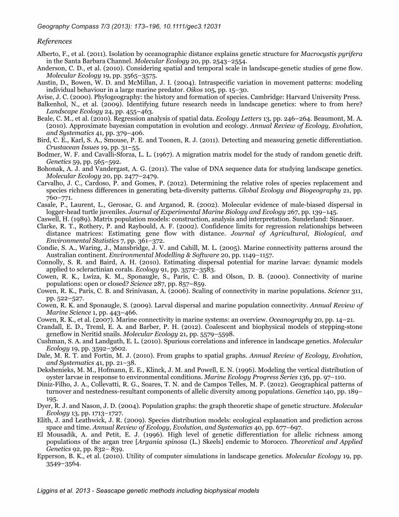
Attributes of species biology will influence marker choice and what is considered to be a sufficient sample size. Many marine organisms are likely to have large effective population sizes resulting from high vagility and fecundity (Hellberg 2009). The process of genetic drift is inversely related to effective population size (Wright 1931). The large population size of many marine organisms, thus, contributes to high levels of genetic diversity within populations and low genetic differentiation between populations (Hedrick 1999), a situation in which statistical tests of population structure are prone to both Type I and Type II error (Waples 1998). These characteristics may necessitate sampling more individuals per population (to capture the asymptote of intra-population genetic diversity) and⁄or the

Fig. 1 Biological characteristics of marine organisms that should be considered in the design, sampling, and analysis of a seascape genetic study. (Note that many of these characteristics are not exclusive to marine organisms, but are also common in terrestrial organisms). Colored bars depict the life stages at which the biological characteristics are relevant (central grey circle: gametes, larvae, juveniles, adults). Local selection during any life stage (dark blue) can influence the interpretation of genetic patterns and genetic measures that assume marker neutrality (the influence of high dispersal ability, ontogenetic habitat shifts, dispersal behavior and the analytical challenges posed by asymmetry in migration are discussed in the main text). Kin aggregation during the larval, juvenile and⁄or adult stages (light blue), can compromise sampling design unless samples are taken sufficiently distant from each other. The ability of some colonial organisms to undergo asexual reproduction (i.e. more than one individual with the same genotype) and colony fusion during juvenile and⁄or adult stages (i.e. one individual with several genotypes; light green) means physically identified ‘individuals’ are not necessarily representative of genetic ‘individuals’ complicating sampling design and violating the Hardy-Weinberg Equilibrium (HWE) model assumption of ‘random mating’. Fluctuating population size (pink) is common in many marine invertebrates and violates the assumption of ‘constant’ and ‘large population size’ in many population genetic models (such as HWE and the island model of migration; the influence of effective population size, species range and patchy or continuous distributions on sampling are discussed in the main text). High mortality during the gametic, larval and⁄or juvenile life stages (light orange) encourages appropriate targetting of life stages, given the study objectives. Non-random mating during the adult and gametic life stages (dark green) violate the assumptions of population genetic models; high variance in reproductive success can lead to small effective population sizes that violate the HWE assumption of ‘large population size’ and can lead to temporal shifts in the genetic composition of age-classes (discussed in the main text, as is the influence of high fecundity, breeding aggregations and temporally segregated reproduction on sampling efforts and analysis). The influence of sex-biased dispersal during the juvenile, adult and⁄or gametic phases (dark orange) are discussed in the main text.



use of more unlinked molecular markers (Waples 1998), permitting analyses based on linkage disequilibria, which are more sensitive to recent isolation between populations than frequency based metrics (see below).

One important caution is that marine or terrestrial studies relying on a single marker (such as mitochondrial DNA, mtDNA) or few markers, must assume that the marker studied is representative of population processes throughout the genome; thus, selective neutrality is implicitly assumed and the large variance in coalescence times among loci is not taken into consideration. In the case of haploid mtDNA (or chloroplast DNA, cpDNA, for algae or sea plants) only properties of female lineages are actually being estimated which may be inappropriate if there is sex-biased dispersal (as in some marine turtles, e.g. Casale et al. 2002). For extensive discussions regarding the appropriate choice of markers, see Manel et al. (2010) and Bohonak & Vandergast (2011).

Focal age-class is important to consider when sampling marine organisms that change their dispersal behaviour, or shift their habitat use over their life time, to avoid obtaining misleading genetic patterns (see Figure 1). The ecologies of age-classes often vary in the marine realm: pelagic larvae develop into benthic adults in many species; and in other species, juveniles will disperse widely and remain solitary whereas adults form social or breeding groups (e.g. leopard seals, Forcada & Robinson 2006). In these examples, sampling one age-class, will provide a different genetic pattern to sampling the other age-class. In some species ontogenetic shifts may be very subtle, for example, larval cardinal fish settle onto rubble and sand areas away from continuous reef sites where adults reside (Finn & Kingsford 1996). These behaviors can confound the interpretation of spatial genetic patterns and co-varying environmental factors if age-class is not taken into account (also see Goldberg & Waits 2010).

The spatial genetic patterns of marine animals are also known to shift over time (Johnson & Black 1982; Planes & Lenfant 2002; Selkoe et al. 2006), potentially due to temporally variable seascape features including currents and⁄or certain reproductive strategies (e.g. high variance in reproductive success, Figure 1). Although this phenomenon is also reported in terrestrial systems (mammals, Scribner et al. 1991; plants, Hossaert-McKey et al. 1996; insects, Guillemaud et al. 2003) it appears to be particularly prevalent in the marine system (Toonen & Grosberg 2011). The occurrence of such temporal genetic shifts encourage consistent timing of sampling (i.e. consistent age-group and timing across locations), and suggest it may be appropriate to sample each population several times, so that the temporal fluctuations in allele frequencies may be captured and accounted for when describing spatial genetic patterns.

INDIVIDUALS OR POPULATIONS?

A fundamental consideration in planning a study is whether individual- or population based sampling and methods of analysis will be employed (Anderson et al. 2010). Individual based analyses use multilocus genotypes to cluster individuals into groups (as in Pritchard 2000) and to infer relatedness and parentage (as in Gerber et al. 2003). Population level analyses typically rely on allele frequencies, although some are based on allelic richness (as in Petit et al. 1998 and Diniz-Filho et al. 2012, see below). In practice many studies, especially those based on multilocus microsatellite genotypes, will use both individual- and population based analyses. However, sampling efforts (individual- or population based) will often be determined by the focal organism’s habit.

Many marine habitats are patchy, therefore sampling strategies familiar to terrestrial systems can also be appropriate to marine systems. In general, if the relevant spatial scale for analysis is small and the species of interest does not have a clumpy distribution but is fairly continuously distributed, then individual-based sampling may be more appropriate. Even over larger distances, individual-based analytical approaches are attractive in that adults and juveniles can be assigned to interbreeding groups based on the genotypes of sampled individuals using parentage analysis and assignment tests (as in Saenz-Agudelo et al. 2009). This ability to delineate groups based on Hardy-Weinberg expectations and linkage disequilibria is useful for species that only aggregate during breeding, but have been sampled outside of the breeding period, or sympatric populations that are segregated by spawning time only.

The primary drawback of individual-based analyses is that multiple unlinked markers (such as microsatellites) are required, whereby power is enhanced by sampling many individuals for many loci (typically 10 or more; for discussion on the effects of sample size, number of markers, and allelic



!!!!"#$%&!'!!(!)*++#,-!./!0.1)23&,#42.1)!,&%&5#14!4.!46&!3&)271!#13!)#+8%217!./!#!)&#)0#8&!7&1&420)!)4*3-9!0.++.1!7&1&420!+&#)*,&)9!#13!).+&!+&46.3)!/.,!46&!#1#%-)2)!./!7&1&420!8#44&,1)!#%.17)23&!7&.7,#8620!#13!&152,.1+&14#%!3#4#!!

:&)271!! ;#+8%217! <&1&420!+&#)*,&)!=!8#44&,1)! :.!)8#42#%!/&#4*,&)!8,&3204!7&1&420!8#44&,1)>!

!;&#)0#8&!/&#4*,&?)!!"##$%&'()#$*$&+$,&'&+-"$.$/&''&+"$01*23$!

"#$%!&'!%#(!)(*(+$,%!'-$%&$*!

$,.!%(/-0)$*!'1$*(2!

!

@#,21&!.,7#12)+?)!!"##$%&'()#$*$&+$45&"$676#)3$!

"#$%!3($%4)('!03!%#(!'-(1&('!

5&0*067!$,.!(10*067!$)(!

)(*(+$,%!%0!%#(!84('%&0,2!

!

"#$%!&'!%#(!6(06)$-#&1!)$,6(!03!%#(!

'-(1&('2!

!

@.%&0*%#,!+#,A&,?)!!

9&,6*(!0)!/4*%&-*(!*01&2!

!

:)(!%#(!*01&!*&,;(.2!

!

"#$%!&'!%#(!/0.(!03!&,#()&%$,1(2!

!

:)(!%#(7!*&;(*7!%0!(+0*+(!&,!$,!

$--)0<&/$%(*7!,(4%)$*!/$,,()!0)!$)(!

%#(7!*&;(*7!%0!

5(!4,.()!'(*(1%&0,2!

!

:)(!%#(7!+$)&$5*(!(,046#!30)!

%#(!301$*!%&/('1$*(2!

!B.1)23&,C!!

9-$%&$*!'1$*(!03!'$/-*&,6!

!

9-$%&$*!$))$,6(/(,%!03!'$/-*&,6!

!

=(-*&1$%&0,!03!'($'1$-(!3($%4)('!

!

>0%(,%&$*!30)!'-$%&$*!$4%010))(*$%&0,!

!

?,.&+&.4$*!0)!-0-4*$%&0,!5$'(.!

'$/-*&,6!

!

@4/5()!03!-0-4*$%&0,'!%0!'$/-*(!

!

:--)0-)&$%(!'$/-*(!'&A(!B%0%$*!$,.!

-()!-0-4*$%&0,C!

!

:--)0-)&$%(!$6(!1*$''!30)!84('%&0,!

!

>0%(,%&$*!30)!4,'$/-*(.!-0-4*$%&0,'!

$,.!-$)%'!03!'-(1&('!)$,6(!

!

:'-(1%'!03!%#(!'-(1&('!5&0*067!$,.!

(10*067!B'((!D&64)(!EC!

!<&1&.%.7-!!

@(%F0);'!

!

>#7*06(,(%&1!%)(('!

!

:25&,)24-!D!EEF24621GG!!

G($'4)('!03!6(,(%&1!.&+()'&%7H!8#I!$**(*&1!)&1#,(''I!$**(*&1!.&+()'&%7I!$,.!

'&/&*$)!.('1)&-%0)'!

!

:2//&,&142#42.1!D!EE$&4F&&1GG!!

G($'4)('!03!6(,(%&1!.&'%$,1(I!

.&33()(,1('!&,!$**(*(!3)(84(,1&('I!

3&<$%&0,!$,.!.&33()(,%&$%&0,!&,.&1('H!

D9JI!KI!K('%I!$,.!'&/&*$)!&,.&1('!

!

<&1&!/%.F!!

:''&6,/(,%!%('%'!

!

L0$*('1(,%!('%&/$%('!

!

!HI8%.,#425&!9"&+'$'#-:)#;#)#+<#=$'#+#4&<$=747>!!!

-#7*06(06)$-#7I!1*4'%()&,6I!5$))&()!.(%(1%&0,!

!

B.,,&%#425&!9"&+'$'#+#4&<$7+=$#+?&)-+@#+47A$@#7"()#"B$"(<5$7"$)#@-4#AC$"#+"#=$=747B$D&-65C"&<7A$=747B$@#7"()#"$=#)&?#=$?&7$A#7"4:<-"4:6745$7+7AC"&"B$)#"&"47+<#$"();7<#"B$<&)<(&4$45#-)C$7+=$;-)$')765$45#-)C>$!

MMF&%#&,NNO!'%$,.$).!4,&+$)&$%(!0)!

/4*%&+$)&$%(!/(%#0.'!

!

MM5(%F((,NNO!G$%)&<!10/-$)&'0,!

/(%#0.'I!G$,%(*!%('%'I!-$)%&$*!G$,%(*!%('%'I!$,.!0%#()!

/4*%&+$)&$%(!$--)0$1#('!%#$%!$110//0.$%(!,0,O

&,.(-(,.(,1(!B&P(P!&'0*$%&0,O57O.&'%$,1(I!&'0*$%&0,O57O

(,+&)0,/(,%I!&'0*$%&0,O57O)('&'%$,1(I!(%1PC!

!J-8.46&)2)!4&)4217!E$6)&-)&$5C6-45#"#"$<7+$D#$&+;-)@#=$("&+'$@#45-="$"(<5$7">$!

Q$5&%$%R,&1#(!/0.(*&,6I!5&0-#7'&1$*!/0.(*&,6!$,.!

'&/4*$%&0,'!

$

F5#$;&4$-;$45#$5C6-45#"&"$4-$45#$-D"#)?#=$'#+#4&<$=747$<7+$D#$7""#""#=$("&+'$(+&?7)&74#$7+=$@(A4&?7)&74#$@#45-="$"(<5$7"$45-"#$7D-?#$$

!

!

richness see Landguth et al. 2012b). Historically, marker development has been financially and technically restrictive, however recent developments in sequencing technologies has made marker development for non-model organisms, such as many marine organisms, considerably more accessible.

For studies interested in longer time frames and sampling over larger distances (which may be necessitated given the patch sizes and distances between patches for seascape features, see Figure 1 in Riginos & Liggins 2013) population-level analyses based on allele frequencies or genealogies can be appropriate and informative. Population-level studies often necessitate sampling fewer individuals per location relative to individual-based methods so that more locations can be included, which can provide greater power for testing the effects of specific seascape features. Population-level analyses also tend to be more flexible with regards to number and type of genetic markers employed and those based on allele frequencies or coalescence will reflect historical averages, and will be less sensitive to recent population subdivision than assignment test methods based on multilocus genotypes.

GENETIC VARIATION WITHIN AND BETWEEN SPATIAL UNITS

Many summary statistics from population genetics may be used as response variables in a seascape genetic study. Genetic response variables can be divided into two main groups: those that provide a metric within a single spatial unit (an individual, population or geographic region) and those that reflect a contrast between spatial units (within and between metrics can be based on individual genotypes or population attributes). For instance, measures of genetic diversity, such as allelic diversity, allelic richness, and heterozygosity are typically expressed as values tied to an explicit spatial unit. In contrast, genetic distances and indices of genetic differentiation (e.g. FST, Wright 1943; Nei’s D, Nei 1972; Dest, Jost 2008) express the difference between spatial units and hence are not linked to a single location but to two or more locations. The differences between populations described by genetic distances primarily reflect the duration of isolation (where genetic drift causes divergence between populations) and the magnitude of isolation (influencing gene flow since separation).

There are many differentiation indices and some are more appropriate than others in certain instances (see Bird et al. 2011; for suggestions). For example, gene flow can be inferred as the inverse



of FST, however the underlying population model assumes no mutation or change in population size (for a complete discussion of factors affecting and appropriate interpretation of this metric see Whitlock & McCauley 1999). Classic population genetic models often have underlying assumptions that will be unrealistic for many marine species (Selkoe et al. 2008) and could lead to the erroneous interpretation of genetic patterns (see Karl et al. 2012, for a discussion on this topic). Recently it has become clear that the inherent variability of genetic markers can also bias some differentiation indices, and this phenomenon is of particular concern in seascape genetics because marine organisms typically display high genetic diversities (see Meirmans & Hedrick 2011, for an overview and suggested solution).

In study species where gene flow should be substantial and⁄or past changes in population size are likely, assignment tests or coalescent methods are more appropriate estimators of genetic connections than those based on genetic distances or differentiation indices (see Marko & Hart 2011, for a recent review of approaches). These methods can infer directionality of gene flow and therefore may be more useful for evaluating asymmetric processes such as transport by currents and investigating source-sink dynamics. However, assignment tests and coalescent approaches are often computationally intensive, and like most applications of genetic distance metrics, usually assume selective neutrality.

The most common metrics used to describe genetic variation within and between are discussed above, but there are other approaches that bridge this distinction and may allow a more nuanced understanding of genetic patterns in the marine system. For instance, Foll & Gaggiotti (2006) have developed a population-specific metric of FST that estimates how distinct a population is relative to all others. The authors were able to use this metric to relate local FST to environmental factors using a linear model (discussed below). Petit et al. (1998) have also suggested a method for partitioning the allelic richness of a population to reflect richness due to novel alleles (divergence), versus those shared with other populations.

Borrowing theory and measures from other fields of science could provide novel approaches to characterising genetic patterns in the sea. For example, Diniz-Filho et al. (2012) presented an approach, whereby differences in allelic richness between populations are partitioned into ‘turnover’ (alleles found in one population and not the other) and differences in richness (when one population’s diversity is nested within the other) in a similar manner to the partitioning of beta-diversity in ecological investigations (e.g. Carvalho et al. 2012). In a very different approach, Dyer & Nason (2004) pioneered a method using graph theory to derive conditional genetic distances (cGD) among populations that take into account the relationship each population has with every other population in the study (for an introduction to graph theoretic representations of genetic data see Garroway et al. 2008; Dale & Fortin 2010). In their method, a population graph is constructed, in which nodes (populations) are only connected by edges when there is genetic covariance (based on the cGDs) between them. One of the several advantages associated with using such ecological or graph theoretic approaches is that it allows access to a well-established suite of analyses.

EVALUATING RELATIONSHIPS BETWEEN ENVIRONMENTAL PREDICTORS AND GENETIC PATTERNS

Seascape genetics, like landscape genetics, is concerned with patterns resulting from dispersal and gene flow (or conversely, barriers that restrict gene flow) and habitat characteristics that modify movements and successful immigration (quality, available space, predators, etc.). The interdisciplinary nature of landscape genetics offers spatially explicit and quantitative methods to assess the relationship between genetic patterns and environmental features and can complement other well-established approaches such as phylogeography (Avise 2000) and habitat or niche modeling (Elith & Leathwick 2009).

A common null hypothesis for genetic patterns established over space has been isolation-by-distance (IBD, Wright 1943, Slatkin 1993; Rousset 2000), where a positive relationship is expected between geographic distance and genetic differentiation for continuously distributed populations (or individuals) that approximate an equilibrium between migration and genetic drift. Indeed, some marine organisms exhibit an IBD pattern (Selkoe & Toonen 2011), but others have an irregular pattern of genetic differentiation (i.e ‘chaotic patchiness’), suggesting seascape features unrelated to Euclidean distance also influence genetic patterns (Riginos & Liggins 2013; Selkoe et al. 2008).

In terrestrial studies, ecological distances are often modeled by weighting the cost (resistance) of traversing various habitats or features and using least-cost-path analyses (as in Spear et al. 2010) or



isolation-by-resistance (McRae 2006) within a geographic information system (GIS). In marine studies, simple over water distance is a commonly used least-cost-path approach, and the increasing availability of remote sensing tools allows investigators to categorize or rank some seascape attributes to create resistance surfaces. Therefore some simplified least-cost-path and isolation-by-resistance approaches can be easily adapted to the seascape. But other, more ecologically meaningful estimates are difficult to implement within a dynamic ocean environment (Galindo et al. 2010). For example, circuit theory (McRae 2008), which takes every possible path among populations into consideration simultaneously, may be inappropriate in systems where dispersal is likely to have directionality. In these instances, biophysical models that use ocean dynamics to capture asymmetries in dispersal, offer a more appropriate method (see next section).

Although ideally a spatial genetic study has a priori hypotheses regarding structuring factors (e.g. distance, barriers and⁄or habitat and environment characteristics), many studies evaluate their genetic patterns against qualitative predictions or use a series of statistics to examine predictions in turn. For example, clustering methods and barrier detection methods identify natural groupings based on genotypes or allele frequencies (see Guillot et al. 2009 for a review of methods) and are frequently used to infer spatial locations of genetic discontinuities; from these putative barriers, potential causes are sometimes qualitatively assessed, largely in a post hoc manner (Anderson et al. 2010; Holderegger & Wagner 2008; Storfer et al. 2010). Whereas such clustering approaches are useful for data exploration and hypothesis generation, their utility for testing alternative or multiple causative factors is limited (and can be misleading, Cushman & Landguth 2010). Some studies employ multiple approaches in series, for example, testing for IBD and also using an analysis of molecular variance (AMOVA, Excoffier et al. 1992) to test the effect of specific barriers, or in combination with isolation-by-environment (IBE) analyses to assess the influence of habitat or environmental characteristics (e.g. Fontaine et al. 2007). These methods have limited utility as they do not consider geographic distance (which can thought of as a source of spatial autocorrelation for IBE analyses), potential barriers and other relevant environmental characteristics in combination.

More rigorous approaches use multivariate frameworks and model testing to infer the importance of specific factors (Balkenhol et al. 2009; Cushman & Landguth 2010; Storfer et al. 2007). For genetic response variables that are tied to a specific location (within variables), linear models can be used, but caution should be taken as spatial autocorrelation may exist between these sites where within variables are measured (see Beale et al. 2010, for example approaches of accounting for this). Similar care should be exercised when using statistics relying on the relationship between locations. These measures violate the statistical assumption of independence, as each single locational unit will be involved in multiple pairwise comparisons. This issue of non-independence has been long recognized in testing for IBD and is often resolved by the use of Mantel tests (Mantel 1967) where significance is assessed via permutation (although there are other methods, e.g. the maximum-likelihood population-effects model, Clarke et al. 2002).

Partial Mantel tests (Smouse 1986) are often used to accommodate multiple predictive factors; however, this method has been suggested to have low power and may be misleading (Balkenhol et al. 2009; Legendre & Fortin 2010; but see Cushman & Landguth 2010). While several other multivariate methods have been proposed in landscape genetics (reviewed by Legendre 2005; Storfer et al. 2007; Balkenhol et al. 2009; Thomassen et al. 2010), many approaches are tailored to certain study systems and thus their methods are not easily transferred. This is particularly the case for seascape genetic analyses where the system may be data depauperate or biologically dependent on very different processes. Nonetheless, the literature of landscape genetics and spatial statistics are inspiring innovative seascape genetic approaches (see Table 1 in Riginos & Liggins 2013 for empirical examples of multivariate seascape assessments).

CORRELATION, NOT CAUSATION

Most landscape genetic studies look for biologically informed correlations but are not able to test for causation. To demonstrate a mechanistic link between a putative spatial factor and genetic variation (either neutral or selective) requires evaluation, such as direct observation of dispersal and reproduction, reciprocal transplantation, common garden experiments, or functional genomics (Feder & Mitchell-Olds 2003; Lowry & Willis 2010). Within the scope of current landscape genetic techniques however, any strong correlation will be bolstered by sound explanation of the organismal biology and



its relation to the environment (comparative approaches can also lend strength to weak patterns, see Selkoe et al. 2010). Hence, making an informed choice of organism, sampling design, and environmental variables or seascape features will enhance any seascape genetic study. In addition, using modeling and simulation approaches such as those described in the next section, one can test their understanding of the mechanisms that lead to the observed spatial genetic patterns (also see Epperson et al. 2010; Thomassen et al. 2010; Landguth et al. 2012a, for simulation approaches in landscape genetics).

Using Biophysical Models in Seascape Genetic Studies

Many seascape features can be quantified using methods similar to those of terrestrial landscape genetics (described in the above section). However, seascape genetic studies can also draw from a complementary set of tools: biophysical models provide methods to simulate individual dispersal, population connectivity, and even genetic patterns across the seascape. In this section we describe the methods of biophysical modeling and their relevant outputs, highlight ways in which genetic and biophysical data may be used together, and point out some considerations for their use.

METHODS OF BIOPHYSICAL MODELING

In a marine context, biophysical models are used to simulate the movement of individuals or propagules by incorporating ocean dynamics derived from hydrodynamic models forced by winds, tides, solar radiance, freshwater inputs, and other characteristics that may influence organismal movement, growth, behavior and survival. These physical factors are then coupled with biological attributes of the focal organism, such as (but not limited to) pelagic larval duration (PLD, Siegel et al. 2003) dispersal behavior (Dekshenieks et al. 1996), mortality (Possingham & Roughgarden 1990) and growth rate (Lett et al. 2010).

There are many approaches, methods, and techniques to model dispersal and population connectivity in the marine system. Each method should incorporate ocean features and the species’ biology within a spatially realistic framework (North et al. 2009). This framework can be accomplished in many ways, ranging from a simple oceanographic distance model of marine population connectivity, which assumes this distance is an adequate proxy for the ‘real’ dispersal process (e.g. White et al. 2010) up to a full spatially- explicit and coupled biophysical model where the individual virtual larvae have unique biological attributes and behavior (e.g. Paris & Chérubin 2007). Adding complexity (or realism) to these models may include incorporating post-settlement processes such as mortality, density-dependence, recruitment, maturity, fecundity, and other population (meta-population) dynamics. A primary challenge is deciding what level of complexity (and spatial resolution) is appropriate for the study questions.

Common biophysical approaches include modeling the dynamics of an entire cohort of swimming virtual larvae as a cloud or plume within a complex ocean (Mora et al. 2011; Treml et al. 2008, 2012) and modeling larvae as individual particles swimming⁄floating in a dynamic ocean (Cowen et al. 2000; Kool et al. 2010; Mitarai et al. 2009). Individual based models (Grimm & Railsback 2005) are becoming more popular and accessible where individual larvae can be assigned properties and behavior allowing them to interact within a simulation environment. These models are also well suited to a wide range of life histories in the sea, from benthic-reef associated organisms (e.g. coral) to highly social, pelagic organisms (e.g. dolphins).

The versatility of biophysical models has been harnessed to inform population dynamics (Possingham & Roughgarden 1990), fisheries stock structure (North et al. 2009), and to estimate larval dispersal distances and patterns (e.g. mussels, Gilg & Hilbish 2003; reef fish, Cowen et al. 2006). To date, biophysical models have been used alongside seascape genetic studies exclusively to model larval dispersal and population connectivity in organisms that have a bi-partite life history. These modeling techniques are particularly attractive for studies that focus on organisms with pelagic gametes or larvae (Leis et al. 2011) as there is often no direct way to observe and quantify propagule movement among populations due to their small size and potentially large distances travelled (but see Jones et al. 2005 for a coupled genetic and physical tracking approach). Here, we review some of the promising methods in which these sources of data can be jointly examined.



COUPLING BIOPHYSICAL MODELS AND SEASCAPE GENETIC DATA

The output of biophysical models relevant to seascape genetic questions can include the dispersal pathway of an individual (or individuals), a species’ or population’s dispersal kernel describing the probability of dispersal with distance from a source, and various connectivity matrices describing the pairwise dispersal characteristics. Common connectivity matrices include the probability matrix, the population transition matrix (Caswell 1989, Cowen et al. 2006), a migration matrix (Bodmer & Cavalli-Sforza 1967), source distribution matrix (Cowen et al. 2007) or a matrix of proportional immigration (Cowen et al. 2006). Which model output is of most interest to geneticists depends on the question and the focal timeframe. For example, genetic assignments tests, or parentage based analyses across one generation or one reproductive event can be compared to modeled dispersal estimates that also represent single dispersal events (Epperson et al. 2010). If the question is concerned more with the long-term average, and⁄or rare events (near the ‘tail’ of a dispersal kernel) such as those measured using mtDNA, then averaging over many model simulations, modeling a cloud of larvae, and⁄or explicitly tracking rare potential events may be important.

There is no straight-forward method to quantitatively test the fit of genetic data and biophysical model outputs. Dispersal matrices derived from biophysical models are pair-wise and directional, thus intuitively they can be compared with pairwise genetic matrices of gene flow (also directional). For genetic measures that are site-specific (within measures), and between measures that are typically symmetrical (e.g. pairwise FST produces a triangular matrix), often the biophysically derived data and⁄or empirical genetic data will be converted to allow comparison.

One useful framework for investigating site-specific, pairwise, aggregate, or network-wide emergent properties of both genetic and biophysically derived data is with graph theory. The structure of complex dispersal or connectivity matrices can be represented as a network allowing graph metrics and properties to be easily calculated (e.g. node centrality, degree, flow patterns and modularity; see Treml et al. 2008; Urban et al. 2009; Treml et al. 2012). For example, Selkoe et al. (2010) used a network representation of their biophysically derived connectivity matrix to calculate a site-specific flow metric, termed ‘eigenvector centrality’ for comparison with various measures of genetic diversity. In another approach Kininmonth et al. (2010) created a network representation of their pairwise FST matrix based on ten microsatellite loci of a brooding coral in an attempt to identify genetic ‘communities’ (i.e. highly connected modules within the network) across the Great Barrier Reef using graph theory. Further, the authors used a network representation of hydrodynamic and distance based models for the same region to cross inform the designation of ‘communities’ based on the likely dispersal of coral propagules.

Another promising means to assess the fit of genetic data with the simulations of a biophysical model is by using the connectivity matrices produced by the biophysical model to explain or predict the empirical genetic data. For example, Kool et al. (2010, 2011) used a matrix approach (based on the matrix model of migration developed by Bodmer & Cavalli-Sforza 1967) to project a time-averaged connectivity matrix forward in time. The projected genetic patterns (genetic diversity and genetic differentiation) could then be compared qualitatively with the empirical genetic patterns over the same seascape (as in Foster et al. 2012). (Also see Galindo et al. 2006, 2010, for a slightly different method).

In high dispersal species it may be preferable to focus on the inter-population genetic measures of gene flow (estimated from coalescent or assignment method approaches as discussed previously), rather than indices of differentiation, to maintain the directionality of relationships. For example, Crandall et al. (2012) used a probabilistic coalescent framework to model gene flow of neritid snails in the Pacific based on the asymmetric connectivity probability matrix of their biophysical model. This method enabled the authors to evaluate the relative performance of the biophysically derived matrix in describing patterns of gene flow relative to other hypothesized and classic population models.

Generally, biophysical simulations and genetic patterns across a common seascape have been in agreement; however there have been cases of inconsistency (Foster et al. 2012; Galindo et al. 2010). Discrepancies between a biophysical model (or any simulation) and observed genetic data can highlight where other processes not already captured may be operating or where the genetic assumptions and⁄or the model assumptions are violated.



CONSIDERATIONS WHEN USING BIOPHYSICAL MODELS WITH GENETIC DATA

While the use of biophysical models and computer simulation approaches in landscape and seascape genetics is very promising (Balkenhol et al. 2009; Epperson et al. 2010), there are some considerations for their use that warrant highlighting. Some of these points are outlined below.

First, modeling methods rely on having reputable physical and biological data (Gallego et al. 2007; Metaxas & Saunders 2009). Ocean circulation models are now available for most of the world’s oceans, but these are often not well resolved at small spatial scales and along complex coastlines (Cowen & Sponaugle 2009), where tides and complex topographies dominate flows. The advancement of satellite data acquisition means there is a multitude of contemporary and comprehensive environmental data available to be used in modeling approaches, however, attention to the biological parameters within these models has been less rigorous (but see Connolly & Baird 2010). This disparity is understandable given that biological parameters are difficult to quantify across different environments and species, and often require a combination of observation and experimentation that can be labor intensive (Metaxas & Saunders 2009).

Second, aligning the resolution and spatio-temporal scale between the biophysical model and genetic model⁄data is essential. Obviously, a biophysical model with resolution defined by a 10 km grid is not suitable, for example, to inform any genetic relationship between seagrass beds separated by 2 km. Likewise, a biophysical model that is based on contemporary ocean currents may inaccurately simulate genetic relationships that have formed over thousands of years (such as those investigated using population sampling and measured using mtDNA markers; but see Crandall et al. 2012).

Third, deciding which parameters are appropriate for inclusion and using the appropriate level of model complexity for the application is important (Gallego et al. 2007; Hannah 2007). Where a biophysical model of larval dispersal per se is used alongside genetic data, one is implicitly interested in the degree to which larval dispersal is driving genetic patterns across the seascape (Kool et al. 2010). In most cases, realized connectivity may also depend on habitat quality, variation in reproduction, population density and local selection (see discussion of environmental variables, above), in addition to the dispersal process. While modeling of post-settlement survival is rare (Hinckley et al. 1996), the addition of selection to biophysical models (as differential mortality or fecundity as functions of the underlying environment and individual genotypes; Epperson et al. 2010) may make them more realistic (Balkenhol et al. 2009). However, modeling approaches can quickly become computationally expensive, lose statistical power and gain uncertainty as more variables are introduced.

Fourth, biophysical models should include some level of model evaluation and parameter validation (Hannah 2007). Physical oceanographic measurements can be used to validate the physical parameters and processes and while it has been suggested that the integrated bio-physical portion can be ‘validated’ using empirical genetic data (Galindo et al. 2006; Hellberg et al. 2002) this may not be appropriate (or possible) due to the mismatch between genetic model assumptions and biophysical modeling assumptions. Genetic data has its own inherent assumptions and inconsistencies particularly over large timeframes (but see assessment of error using probabilistic coalescent frameworks in Crandall et al. 2012). To build confidence in a biophysical model, the sensitivity of predicted and observed data matches to changing a variety of parameters should be explored (Treml et al. 2012). There are also several methods available to aid in model selection (see Hartig et al. 2011), such as Approximate Bayesian Computing (Beaumont 2010) and pattern-oriented modeling (Grimm & Railsback 2012; Grimm et al. 2005). However, as with all modeling approaches, the user must also be aware that, strictly speaking, the biophysical models cannot be validated. The model is necessarily a simplification of the natural system with a finite number of parameters and processes, and therefore will not ‘truthfully’ represent the system (Oreskes et al. 1994). As a result, model evaluation, as opposed to ‘validation’, is a key component in integrating models and empirical data.

Lastly, biophysical modeling is quite technical and requires substantial expertise in physical oceanography and marine ecology, and available⁄adequate computing resources. Although biophysical models are being made more accessible (see Condie et al. 2005; Roberts et al. 2010), their use requires sound data, appropriate parameters, and thorough understanding of the inherent assumptions, and what the model output represents.



Conclusions

Undertaking a seascape genetic study requires an understanding of the focal organisms’ biology and how it is likely to interact with the seascape features of interest (see Figure 1). Using well-considered sampling design (i.e. spatial arrangement, individuals or populations) and genetic methods (i.e. choice of marker, methods of analyses) is invaluable in teasing apart the relative influences of competing seascape features (see Table 1). Methods of analysis are becoming more rigorous and spatially explicit offering better opportunities for the interpretation of the genetic patterns, however taking an informed approach to any seascape genetic question and study design cannot be underestimated.

Seascape genetics is increasingly forming a discipline distinct from ‘‘landscape genetics’’ (Riginos & Liggins 2013). The biology of marine organisms and the marine environment inspire questions that are often distinct from questions asked of terrestrial systems, some of which require the development of new techniques and the melding of different areas of expertise. The topic of greatest marine-focused development relevant to landscape genetics has been biophysical modeling. Despite there being several challenges remaining, the integration of biophysical modeling and seascape genetics is exciting not only for the knowledge that it will generate about the marine system, but because it encourages collaboration and mutual understanding between experts and across disciplines.

Glossary

A Molecular Analysis Of Variance (AMOVA): a method of partitioning hierarchical genetic diversity into groupings that is analogous to an analysis of variance: proportions of variance are expressed according to hierarchies, such as within and among populations, within and among groups etc. (Excoffier et al. 1992).

Alleles: different forms (polymorphisms) of the same marker (locus).Allelic diversity: a measure of how many alleles are in a population for a locus. It can be expressed as a

number or a proportion.Allele frequencies: the frequency of an allele in a population is called the allele frequency. Genetically

distinct populations will differ in their composition or frequency of alleles.Allelic richness: the number or proportion of alleles within a population with a correction for sample size

bias (El Mousadik & Petit 1996).Assignment tests: a statistical approach that assigns an individual to the sampled population from which

its genotype is most likely to be derived.Bayesian: a field of statistics that combines data with prior information about parameter values in order to

derive posterior probabilities of different models or parameter values.Benthic: marine organisms that live on, in or attached to the sea floor.Biophysical modeling: couples physical and biological data to model a biological system.Bi-partite life history: many marine organisms have a bi-partite life history, whereby they have a

planktonic dispersive early stage (as gametes, eggs and⁄or larvae), after which they ‘settle’ (and metamorphose) to resume a benthic juvenile and adult stage.

Bottleneck (genetic): a population bottleneck occurs when the effective population size, Ne, decreases substantially. A bottleneck causes an immediate decrease in genetic diversity, promoting stochastic genetic drift.

Coalescence (times): the event (or timing) of common ancestry for two alleles found in the present day population. For example, mtDNA of two siblings coalesces in the previous generation as they both received their copies from their mother.

Chloroplast DNA (cpDNA): cytoplasmic elements containing a circular genome. They share many properties with mtDNA, including maternal transmission, but are only found in algae and plants.

Circuit theory: electrical circuit theory that can be used to model connectivity. Models based on circuit theory have the advantage of being able to evaluate the contributions of multiple dispersal pathways, simultaneously considering redundancy in a connection and also increasing connectivity via multiple pathways (McRae 2008).

Dispersal kernel: a probability density function describing how far individuals disperse from their place of origin. The mode has demographic relevance, whereas the tail is relevant on an evolutionary level (Paris & Chérubin 2007).

Effective population size (Ne): an index of how many individuals are passing on their genetic material. It represents the size of the ‘‘ideal population’’ that would lose variation or ‘drift’ at the same rate observed in the real biological population. Ne is an important parameter in population genetics and can be used to model and predict drift and changes in genetic diversity.



Euclidean geographic distance: the shortest path between two geographic points; may account for the curvature of the earth.

FST: FST describes the proportion of genetic variation that is attributable to variation between populations relative to the total variation among all populations (Wright 1943). There are many specific methods for calculating FST and its derivatives (see Meirmans & Hedrick 2011).

Gene flow: the spread of alleles⁄genes from one population to another resulting from migrant individuals moving among populations. In the absence of selection and drift, gene flow would eventually homogenize allele frequencies across populations. Mathematically gene flow is expressed as Nem, the product of the effective population size (Ne) and migration rate (m). Nem is the number of migrant individuals per generation.

Genealogy: a genealogy portrays the ancestral relationship between individuals and is usually presented in a tree-like form. Common usages of genealogies include tracing the inheritance of alleles across generations, or a genealogy can represent a summary of evolutionary changes for a locus whereby splitting events on the tree represent mutation creating a new variant.

Genetic admixture: when interbreeding occurs between two genetically differentiated populations, the resultant population and individuals are considered ‘‘admixed’’. Admixture is a common source of linkage disequilibria.

Genetic distance: a measure of genetic distinctness between populations, which should be proportional to the amount of time since the populations diverged (assuming the loci are neutral and there has no gene flow following divergence). There are many specific methods for calculating genetic distance, for instance by changing the weightings among mutational models (Nei & Kumar 2000).

Genetic drift: changes in allele frequencies caused by random effects of sampling when gametes are passed from one generation to the next. Genetic drift is the main process leading to neutral genetic structure and is inversely proportional to effective population size; small populations experience greater genetic drift.

Genetic variation or genetic diversity: a measure of heritable attributes, generally but not exclusively at the DNA level (i.e. single nucleotide polymorphisms, haplotypes, alleles, etc.). Genetic variation is quantifiable within individuals (diploid heterozygous individuals have different alleles at the same loci), among individuals, among populations, and among species.

Genomics: the study of the function of genes and the structure and evolution of genomes.Genotype: the precise combination of alleles (typically across many loci) found in an individual.Graph theory: a body of mathematical knowledge in which structural units are depicted as nodes with

relationships between them depicted as links. Graph theory provides a flexible framework that can clarify the relationship between structures and processes, including the mechanisms of configuration effects and compositional differences.

Habitat⁄niche modeling: the process of using algorithms to predict the distribution of species in geographic space based on a mathematical representation of their known distribution in environmental space (i.e. habitat⁄niche).

Haplotype: a stretch of DNA that may include multiple polymorphic sites. Most frequently, the term is used to refer specifically to DNA sequences from haploid markers (such as mtDNA or cpDNA). Technically, however, the two copies (alleles) of nuclear diploid DNA sequences are also haplotypes.

Haplotype diversity: a measure of how many haplotypes are in a population for a locus. May be expressed as a number or a proportion.

Hardy-Weinberg Equilibrium (HWE): a population genetic principle stating that allele and genotype frequencies reach equilibrium within a single generation and remain constant, assuming that a population is large (unlimited), has random mating, no genetic drift, no selection, no gene flow, and no mutation. HWE is often an assumption underlying population genetic analysis, and is a useful null model often used to infer assortative mating, selection, or migration.

Heterozygosity (He): a measure of genetic diversity. Within an individual, heterozygosity is the proportion of loci with two different alleles. Within populations, heterozygosity can be expressed as observed or expected heterozygosity. Observed heterozygosity (Ho) is the proportion of individuals in the population that are heterozygous (for the locus or loci of interest). The expected heterozygosity (He) is the heterozygosity that would be observed if there was complete random mating; it is calculated from allele frequencies rather than observed genotypes.

Island model of migration: a population genetic model that combines the effects of gene flow and genetic drift. The model assumes: there is an infinite number of populations, populations each have a constant size (N), individuals migrate among populations at a constant rate of m, every individual is equally likely to migrate, there is no mutation or selection and every population is in a migration-genetic drift equilibrium (Wright 1931).

Isolation-by-distance (IBD): the pattern of local genetic differences that can accumulate under geographically restricted dispersal. It is based on stepping stone model of migration, and assumes that migration



between populations occurs at the same rate as genetic drift within populations (e.g. a migration-drift equilibrium). IBD results from the expectation that genetic distance will increase with geographic distance (Wright 1943).

Isolation-by-environment (IBE): the pattern of local genetic differences that can accumulate due to the local environment. A pattern of genetic differences between populations that are correlated with environmental differences in their habitats is referred to as an IBE pattern (Mendez et al. 2010).

Isolation-by-resistance: the pattern of local genetic differences that can accumulate due to the landscape resistance, which results from different landscape elements filtering gene flow in differing ways (McRae 2006).

Landscape genetics: a field of study that quantifies the effect of landscape and⁄or environmental characteristics on gene flow or spatial genetic variation (Storfer et al. 2007).

Least-cost-path analyses (LCP): with least-cost-path analysis, connectivity values are based on the path of least resistance between any two landscape elements.

Lineage: an evolutionary lineage is a group of species, or populations or gene variants that form an exclusive line of descent, often represented in a phylogenetic tree or network.

Linear model: a mathematical model describing the effect of one or more predictive variables on an observed response variable. In land- or seascape genetics, environmental features usually comprise predictive variables and a genetic metric is the response variable.

Linkage disequilibria: a pattern found when alleles from different loci do not assort independently. Linkage equilibrium (the independence of loci) is assumed in many population genetic methods. Linkage disequilibrium can be caused by physical linkage (i.e. loci are close together on the genome) or by demographic events such as bottlenecks followed by rapid expansion, mixing between previously isolated groups, extreme drift in small populations, and selection.

Locus (plural: loci): a locus is any region of the genome. The term is vague with regards to size and function of the genomic region in question.

Mantel tests: a permutation-based statistical test describing the correlation between two distance or dissimilarity matrices (Mantel 1967). A partial Mantel simultaneously accounts for the effects of other distance matrices (Smouse 1986).

Marker (genetic): a genetically heritable and variable trait or locus.Microevolutionary processes: evolutionary processes including mutation, selection, gene flow, and

genetic drift that lead to a change in allele composition and allele frequencies within a population over time.Microsatellite (loci): simple DNA sequence repeats, typically of 2–6 base pairs motifs. Both alleles are

discernable for diploid organisms and microsatellites are well-known for their high rate of mutation making them well-suited for inferring demographic processes over relatively recent timescales.

Migration: in population genetics, migration (m) is the rate (i.e. proportion of the total population) at which migrants are exchanged among populations.

Mitochondrial DNA (mtDNA): cytoplasmic elements that contain a small circular genome and are transmitted from mothers to their progeny. Genetic studies of animals frequently focus on the mtDNA because it is easy to sequence and also maternal transmission reduces the total copies in a population relative to nuclear genes (as mtDNA is both haploid and only persists through female lineages). The smaller population size of mtDNA relative to nuclear loci means that genetic drift acts more efficiently changing allele frequencies in populations more rapidly (albeit over evolutionary time scales of tens of thousands or more years).

Mutation: an alteration to the genome, which creates new alleles. The rate and process of mutation varies by locus. A point mutation alters the nucleotide sequence for a single nucleotide, insertions add new nucleotides, and deletions remove nucleotides.

Neutral locus: a locus evolving without the influence of selection. Although selection cannot be statistically detected for many loci and neutrality is therefore assumed in these instances, in reality it is unclear whether any locus is ever absolutely neutral. Most population genetic methods of inferring gene flow assume (approximate) neutrality.

Neutral population processes: gene flow, genetic drift and mutation are neutral population processes. If there is no selection and loci are neutral, only drift and gene flow affect the fate of a new allele created by mutation.

Parentage analysis: a statistical approach that assigns an individual to parents or parental populations based on their genotypes.

Pelagic larval duration (PLD): the length of time a larva spends in the pelagic environment after hatching and before settling onto a reef and⁄or metamorphosing.

Pelagic: marine organisms (or their gametes) that live in the open sea, or the water column away from the benthos.



Population genetics: a field of biology that studies the genetic composition of populations, and the changes in genetic composition that result from microevolutionary processes.

Population (genetic) structure: a descriptor of the tendency for individuals within a population to be more genetically similar than individuals from different populations. Species biology and geographical features influence the degree of population genetic structuring found across geographic space (via microevolutionary processes).

Phylogeography: a field of study concerned with the microevolutionary and geographical processes governing the geographic distributions of genealogical lineages within and among closely related species (Avise 2000).

Recruitment: the process and phase by which ‘settlers’ in a marine population successfully recruit into the adult population.

Seascape genetics: an area of study that evaluates the effects of spatially variable structural and environmental features on genetic patterns of marine organisms; equivalent to marine landscape genetics.

Selection: the non-random survival or mortality (of individuals) associated with a specific heritable trait(s). Various statistical tests can infer the imprint of selection on specific loci.

Self-recruitment: also called local replenishment; recruitment into a population from itself.Settlement: the process of pelagic larvae transitioning into a benthic life style. Metamorphosis occurs

during the settlement process.Source-sink dynamics: a meta-population construct where a ‘source’ is a population in which the net

export of individuals is greater than the net import of individuals; the reverse is a ‘sink’.Unlinked markers: loci that are not physically linked. Using unlinked markers increases the statistical

power to infer past population history and locus-specific selection.

Acknowledgements

We thank HP Possingham, ED Crandall, JA Kupfer and one anonymous reviewer for comments that substantially improved the manuscript. LL was supported by an Australian Postgraduate Award from the Australian Government and a Queensland Government Smart Futures PhD Scholarship. Many of the ideas discussed here grew out of work funded by the Australian Research Council (DP0878306, to CR), the Sea World Research & Rescue Foundation (SWR⁄1⁄2012, to CR and LL), a Paddy Pallin Foundation and The Foundation for National Parks & Wildlife Science Grant, an Ecological Society of Australia Student Research Grant, the Lerner Gray Memorial Fund of the American Museum of Natural History, a Great Barrier Reef Marine Park Authority’s Science for Management Award, and an Explorer’s Club Exploration Fund (to LL).

Short Biographies

Libby Liggins is a PhD candidate at the University of Queensland within the School of Biological Sciences. Her current research takes a phylogeographic and population genetic approach to understanding connectivity among coral reef populations in several species common to the Austral-West-Pacific region. Specifically, she is interested in understanding the drivers of spatial genetic patterns across this region and shifts in the genetic composition of populations across life history stages and through time. Libby completed her BSc in Ecology, Biodiversity and Environmental Science and MSc in Conservation Biology within the School of Biological Sciences at Victoria University of Wellington.

Eric Treml’s research is focused primarily on the spatial ecology of marine systems, testing hypotheses regarding marine population connectivity (dispersal corridors and barriers), and exploring the implications for marine conservation and ecosystem-based management. This research integrates dynamic modeling, spatial analysis with GIS, graph theory, and population genetic techniques. Eric is currently a Research Fellow at the University of Melbourne and recently completed a World Wildlife Fund Fuller Fellowship at the University of Queensland. His academic training includes a BSc and MSc in marine biology and ecology and a PhD from Duke University’s Nicholas School of the Environment.

Cynthia Riginos has a long-standing interest in the ecological and evolutionary implications of planktonic larval dispersal. She is currently a Senior Lecturer at the University of Queensland in the School of Biological Sciences. She teaches first year Genetics, second year Ecology, and a senior



undergraduate class in Ecological and Evolutionary Genetics. She and her research group work on a wide array of organisms (even some that lack planktonic larvae), including reef fishes, cartilaginous fishes, mollusks, echinoderms, ascidians, and insects. Current topics of interest include applying spatially explicit methods to marine population genetics and using genomic tools to measure post-settlement selection. Cynthia received her MS and PhD from the University of Arizona in Ecology and Evolutionary Biology and was a post-doctoral fellow for many years at Duke University in the Department of Biology.

Further reading

SPECIAL ISSUE on landscape genetics (2010). Molecular Ecology 19 (17), pp. 3489–3835. A collection of reviews and original articles related to landscape genetics.

Bohonak, A. J. and Vandergast, A. G. (2011). The value of DNA sequence data for studying landscape genetics. Molecular Ecology 20, pp. 2477–2479. A discussion of genetic markers and methods of analysis in landscape genetics.

Cowen, R. K. and Sponaugle, S. (2009). Larval dispersal and marine population connectivity. Annual Review of Marine Science 1, pp. 443–466. A review on larval dispersal and marine connectivity including biophysical models.

Gallego, A., North, E. W., Petitgas, P. and Browman. H. I. (idea and coordination) (2007) Advances in modelling physical-biological interactions in fish early life history. Marine Ecology Progress Series THEME SECTION 347, pp. 121–306. A collection of reviews and original articles related to modeling the fish early life history.

Guillot, G., Leblois, R. L., Coulon, A. L. and Frantz, A. C. (2009). Statistical methods in spatial genetics. Molecular Ecology 18, pp. 4734–4756. A review of methods for spatial analysis.

Hellberg, M. E. (2009). Gene flow and isolation among populations of marine animals. Annual Review of Ecology, Evolution and Systematics 40, pp. 291–310. A general review of population genetics of marine organisms.

Holderegger, R. and Wagner, H. H. (2008). Landscape Genetics. BioScience 59, pp. 199–207. A general review of landscape genetics.

Manel, S., Schwartz, M. K., Luikart, G. and Taberlet, P. (2003). Landscape genetics: combining landscape ecology and population genetics. Trends in Ecology & Evolution 18, pp. 189–197. A general review of landscape genetics.

Marko, P. B. and Hart, M. W. (2011). The complex analytical landscape of gene flow inference. Trends in Ecology & Evolution 26, pp. 448–456. A recent review of analytical approaches for estimating geneflow.

North, E. W., Gallego, A. and Petitgas, P. 2009. Manual of recommended practices for modelling physical-biological interactions in fish early-life. Copenhagen: International council for the Exploration of the Sea cooperative Research Report 295, pp. 1–112. A manual of recommended practices for modeling the early life history of fish.

Roberts, J. J., Best, B. D., Dunn, D. C., Treml, E. A. and Halpin, P. N. (2010). Marine Geospatial Ecology Tools: an integrated framework for ecological geoprocessing with ArcGIS, Python, R, MATLAB, and C++. Environmental Modelling & Software 25, pp. 1197–1207. A description of the Marine Geospatial Ecology Tools package that hosts a publicly available biophysical model capable of evaluating the impact of biological and environmental parameters on marine population connectivity across various seascapes.

Selkoe, K. A., Henzler, C. M. and Gaines, S. D. (2008). Seascape genetics and the spatial ecology of marine populations. Fish and Fisheries 9, pp. 363–377. A general review of seascape genetics.

Storfer, A., Murphy, M. A., Evans, J. S., Goldberg, C. S., Robinson, S., Spear, S. F., Dezzani, R., Delmelle, E., Vierling, L. and Waits, L. P. (2007). Putting the ‘landscape’ in landscape genetics. Heredity 98, pp. 128–142. An extended discussion of sampling approaches and design considerations in landscape genetics.



References

Alberto, F., et al. (2011). Isolation by oceanographic distance explains genetic structure for Macrocystis pyrifera in the Santa Barbara Channel. Molecular Ecology 20, pp. 2543–2554.

Anderson, C. D., et al. (2010). Considering spatial and temporal scale in landscape-genetic studies of gene flow. Molecular Ecology 19, pp. 3565–3575.

Austin, D., Bowen, W. D. and McMillan, J. I. (2004). Intraspecific variation in movement patterns: modeling individual behaviour in a large marine predator. Oikos 105, pp. 15–30.

Avise, J. C. (2000). Phylogeography: the history and formation of species. Cambridge: Harvard University Press. Balkenhol, N., et al. (2009). Identifying future research needs in landscape genetics: where to from here?

Landscape Ecology 24, pp. 455–463. Beale, C. M., et al. (2010). Regression analysis of spatial data. Ecology Letters 13, pp. 246–264. Beaumont, M. A.

(2010). Approximate bayesian computation in evolution and ecology. Annual Review of Ecology, Evolution, and Systematics 41, pp. 379–406.

Bird, C. E., Karl, S. A., Smouse, P. E. and Toonen, R. J. (2011). Detecting and measuring genetic differentiation. Crustacean Issues 19, pp. 31–55.

Bodmer, W. F. and Cavalli-Sforza, L. L. (1967). A migration matrix model for the study of random genetic drift. Genetics 59, pp. 565–592.

Bohonak, A. J. and Vandergast, A. G. (2011). The value of DNA sequence data for studying landscape genetics. Molecular Ecology 20, pp. 2477–2479.

Carvalho, J. C., Cardoso, P. and Gomes, P. (2012). Determining the relative roles of species replacement and species richness differences in generating beta-diversity patterns. Global Ecology and Biogeography 21, pp. 760–771.

Casale, P., Laurent, L., Gerosac, G. and Arganod, R. (2002). Molecular evidence of male-biased dispersal in logger-head turtle juveniles. Journal of Experimental Marine Biology and Ecology 267, pp. 139–145.

Caswell, H. (1989). Matrix population models: construction, analysis and interpretation. Sunderland: Sinauer. Clarke, R. T., Rothery, P. and Raybould, A. F. (2002). Confidence limits for regression relationships between

distance matrices: Estimating gene flow with distance. Journal of Agricultural, Biological, and Environmental Statistics 7, pp. 361–372.

Condie, S. A., Waring, J., Mansbridge, J. V. and Cahill, M. L. (2005). Marine connectivity patterns around the Australian continent. Environmental Modelling & Software 20, pp. 1149–1157.

Connolly, S. R. and Baird, A. H. (2010). Estimating dispersal potential for marine larvae: dynamic models applied to scleractinian corals. Ecology 91, pp. 3572–3583.

Cowen, R. K., Lwiza, K. M., Sponaugle, S., Paris, C. B. and Olson, D. B. (2000). Connectivity of marine populations: open or closed? Science 287, pp. 857–859.

Cowen, R. K., Paris, C. B. and Srinivasan, A. (2006). Scaling of connectivity in marine populations. Science 311, pp. 522–527.

Cowen, R. K. and Sponaugle, S. (2009). Larval dispersal and marine population connectivity. Annual Review of Marine Science 1, pp. 443–466.

Cowen, R. K., et al. (2007). Marine connectivity in marine systems: an overview. Oceanography 20, pp. 14–21.Crandall, E. D., Treml, E. A. and Barber, P. H. (2012). Coalescent and biophysical models of stepping-stone

geneflow in Neritid snails. Molecular Ecology 21, pp. 5579–5598. Cushman, S. A. and Landguth, E. L. (2010). Spurious correlations and inference in landscape genetics. Molecular

Ecology 19, pp. 3592–3602. Dale, M. R. T. and Fortin, M. J. (2010). From graphs to spatial graphs. Annual Review of Ecology, Evolution,

and Systematics 41, pp. 21–38. Dekshenieks, M. M., Hofmann, E. E., Klinck, J. M. and Powell, E. N. (1996). Modeling the vertical distribution of

oyster larvae in response to environmental conditions. Marine Ecology Progress Series 136, pp. 97–110. Diniz-Filho, J. A., Collevatti, R. G., Soares, T. N. and de Campos Telles, M. P. (2012). Geographical patterns of

turnover and nestedness-resultant components of allelic diversity among populations. Genetica 140, pp. 189–195.

Dyer, R. J. and Nason, J. D. (2004). Population graphs: the graph theoretic shape of genetic structure. Molecular Ecology 13, pp. 1713–1727.

Elith, J. and Leathwick, J. R. (2009). Species distribution models: ecological explanation and prediction across space and time. Annual Review of Ecology, Evolution, and Systematics 40, pp. 677–697.

El Mousadik, A. and Petit, E. J. (1996). High level of genetic differentiation for allelic richness among populations of the argan tree [Argania spinosa (L.) Skeels] endemic to Morocco. Theoretical and Applied Genetics 92, pp. 832– 839.

Epperson, B. K., et al. (2010). Utility of computer simulations in landscape genetics. Molecular Ecology 19, pp. 3549–3564.



Excoffier, L., Smouse, P. and Quattro, J. M. (1992). Analysis of molecular variance inferred from metric distances among DNA haplotypes: application to human mitochondrial DNA restriction data. Genetics 131, pp. 479–491.

Feder, M. E. and Mitchell-Olds, T. (2003). Evolutionary and ecological functional genomics. Nature Reviews 4, pp. 649–655.

Finn, M. D. and Kingsford, M. J. (1996). Two-phase recruitment of Apogonids (Pisces) on the Great Barrier Reef. Marine and Freshwater Research 47, pp. 423–432.

Foll, M. and Gaggiotti, O. (2006). Identifying the environmental factors that determine the genetic structure of populations. Genetics 174, pp. 875–891.

Fontaine, M. C., et al. (2007). Rise of oceanographic barriers in continuous populations of a cetacean: the genetic structure of harbour porpoises in Old World waters. BMC Biology 5, doi: 10.1186/17417007-5-30.

Forcada, J. and Robinson, S. L. (2006). Population abundance, structure and turnover estimates for leopard seals during winter dispersal combining tagging and photo-identification data. Polar Biology 29, pp. 1052–1062.

Foster, N. L., et al. (2012). Connectivity of Caribbean coral populations: complementary insights from empirical and modelled gene flow. Molecular Ecology 21, pp. 1143–1157.

Galindo, H. M., et al. (2010). Seascape genetics along a steep cline: using genetic patterns to test predictions of marine larval dispersal. Molecular Ecology 19, pp. 3692–3707.

Galindo, H., Olson, D. and Palumbi, S. R. (2006). Seascape genetics: a coupled oceanographic-genetic model predicts population structure of Caribbean corals. Current Biology 16, pp. 1622–1626.

Gallego, A., North, E. W. and Petitgas, P. (2007). Introduction: status and future of modelling physical-biological interactions during the early life of fishes. Marine Ecology Progress Series 347, pp. 121–126.

Garroway, C. J., Bowman, J., Carr, D. and Wilson, P. J. (2008). Applications of graph theory to landscape genetics. Evolutionary Applications 1, pp. 620–630.

Gerber, S., Chabrier, P. and Kremer, A. (2003). FAMOZ: a software for parentage analysis using dominant, codominant and uniparentally inherited markers. Molecular Ecology Notes, 3, pp. 479–481.

Gerlach, G., et al. (2007). Smelling home can prevent dispersal of reef fish larvae. Proceedings of the National Academy of Sciences of the United States of America 104, pp. 858–863.

Gilg, M. R. and Hilbish, T. J. (2003). The geography of marine larval dispersal: coupling genetics with fine-scale physical oceanography. Ecology 84, pp. 2989–2998.

Goldberg, C. S. and Waits, L. P. (2010). Quantification and reduction of bias from sampling larvae to infer population and landscape genetic structure. Molecular Ecology Resources 10, pp. 304–313.

Grimm, V. and Railsback, S. F. (2005). Individual-based Modeling and Ecology. Princeton: Princeton University Press.

Grimm, V. and Railsback, S. F. (2012). Pattern-oriented modelling: a ‘multi-scope’ for predictive systems ecology. Philosophical Transactions of the Royal Society of London. Series B, Biological sciences 367, pp. 298–310.

Grimm, V., et al. (2005). Pattern-oriented modeling of agent-based complex systems: lessons from ecology. Science 310, pp. 987–991.

Guillemaud, T., Mieuzet, L. and Simon, J. C. (2003). Spatial and temporal genetic variability in French populations of the peach-potato aphid, Myzus persicae. Heredity 91, pp. 143–152.

Guillot, G., Leblois, R. L., Coulon, A. L. and Frantz, A. C. (2009). Statistical methods in spatial genetics. Molecular Ecology 18, pp. 4734–4756.

Hannah, C. G. (2007). Future directions in modelling physical–biological interactions. Marine Ecology Progress Series 347, pp. 301–306.

Hartig, F., et al. (2011). Statistical inference for stochastic simulation models-theory and application. Ecology Letters 14, pp. 816–827.

Hedrick, P. W. (1999). Highly variable loci and their interpretation in evolution and conservation. Evolution 53, pp. 313–318.

Hellberg, M. E. (2009). Gene flow and isolation among populations of marine animals. Annual Review of Ecology, Evolution and Systematics 40, pp. 291–310.

Hellberg, M. E., Burton, R. S., Neigel, J. E. and Palumbi, S. R. (2002). Genetic assessment of connectivity among marine populations. Bulletin of Marine Science 70, pp. 273–290.

Hinckley, S., Hermann, A. J. and Megray, B. A. (1996). Development of a spatially explicit, individual-based models of marine fish early life history. Marine Ecology Progress Series 139, pp. 47–68.

Holderegger, R. and Wagner, H. H. (2008). Landscape Genetics. BioScience 59, pp. 199–207.Hossaert-McKey, M., et al. (1996). The evolving genetic history of a population of Lathyrus sylvestris: evidence

from temporal and spatial genetic structure. Evolution 50, pp. 1808–1821. Johnson, M. S. and Black, R. (1982). Chaotic genetic patchiness in an intertidal limpet, Siphonaria sp. Marine

Biology 70, pp. 157–164.



Jones, G. P., Planes, S. and R., T. S. (2005). Coral reef fish larvae settle close to home. Current Biology 15, pp. 1314–1318.

Jost, L. (2008). GST and its relatives do not measure differentiation. Molecular Ecology 17, pp. 4015–4026. Karl, S. A., Toonen, R. J., Grant, W. S. and Bowen, B. W. (2012). Common misconceptions in molecular ecology:

echoes of the modern synthesis. Molecular Ecology 21, pp. 4171–4189.Kingsford, M. J., et al. (2002). Sensory environments, larval abilities and local self-recruitment. Bulletin of

Marine Science 70, pp. 309–340. Kininmonth, S., van Oppen, M. J. H. and Possingham, H. P. (2010). Determining the community structure of the

coral Seriatopora hystrix from hydrodynamic and genetic networks. Ecological Modelling 221, pp. 2870–2880.

Kool, J. T., Paris, C. B., Andréfouët, S. and Cowen, R. K. (2010). Complex migration and the development of genetic structure in subdivided populations: an example from Caribbean coral reef ecosystems. Ecography 33, pp. 597–606.

Kool, J. T., Paris, C. B., Barber, P. H. and Cowen, R. K. (2011). Connectivity and the development of population genetic structure in Indo-West Pacific coral reef communities. Global Ecology and Biogeography 20, pp. 695–706.

Landguth, E. L., Cushman, S. A. and Johnson, N. A. (2012a). Simulating natural selection in landscape genetics. Molecular Ecology Resources 12, pp. 363–368.

Landguth, E. L., et al. (2012b). Effects of sample size, number of markers, and allelic richness on the detection of spatial genetic pattern. Molecular Ecology Resources 12, pp. 276–284.

Legendre, P. (1993). Spatial autocorrelation: trouble or new paradigm? Ecology 74, pp. 1659–1673.Legendre, P. (2005). Analyzing beta diversity: partitioning the spatial variation of community composition data.

Ecological Monographs 75, pp. 435–450. Legendre, P. and Fortin, M.-J. (2010). Comparison of the Mantel test and alternative approaches for detecting

complex multivariate relationships in the spatial analysis of genetic data. Molecular Ecology Resources 10, pp. 831–844.

Leis, J. M., van Herwerden, L. and Patterson, H. M. (2011). Estimating connectivity in marine fish populations: what works best? Oceanography and Marine Biology 49, pp. 193–234.

Lett, C., Ayata, S.-D., Huret, M. and Irisson, J.-O. (2010). Biophysical modelling to investigate the effects of climate change on marine population dispersal and connectivity. Progress in Oceanography 87, pp. 106–113.

Levin, S. A., Muller-Landau, H. C., Nathan, R. and Chave, J. (2003). The ecology and evolution of seed dispersal: a theoretical perspective. Annual Review of Ecology, Evolution, and Systematics 34, pp. 575–604.

Lowry, D. B. and Willis, J. H. (2010). A widespread chromosomal inversion polymorphism contributes to a major life-history transition, local adaptation, and reproductive isolation. PLoS Biology 8(9), e1000500. doi: 10.1371/journal.pbio.1000500.

Manel, S., Schwartz, M. K., Luikart, G. and Taberlet, P. (2003). Landscape genetics: combining landscape ecology and population genetics. Trends in Ecology & Evolution 18, pp. 189–197.

Manel, S., et al. (2010). Perspectives on the use of landscape genetics to detect genetic adaptive variation in the field. Molecular Ecology 19, pp. 3760–3772.

Mantel, N. (1967). The detection of disease clustering and a generalized regression approach. Cancer Research 27, pp. 209–220.

Marko, P. B. and Hart, M. W. (2011). The complex analytical landscape of gene flow inference. Trends in Ecology & Evolution 26, pp. 448–456.

McRae, B. H. (2006). Isolation by resistance. Evolution 60, pp. 1551–1561. McRae, B. H. (2008). Using circuit theory to model connectivity in ecology, evolution and conservation. Ecology

89, pp. 2712–2724. Meirmans, P. G. and Hedrick, P. W. (2011). Assessing population structure: FST and related measures. Molecular

Ecology Resources 11, pp. 5–18. Mendez, M., et al. (2010). Isolation by environmental distance in mobile marine species: molecular ecology of

franciscana dolphins at their southern range. Molecular Ecology 19, pp. 2212–2228.Metaxas, A. and Saunders, M. (2009). Quantifying the ‘‘bio-’’ components in biophysical models of larval

transport in marine benthic invertebrates: advances and pitfalls. Biological Bulletin 216, pp. 257–272. Mitarai, S., et al. (2009). Quantifying connectivity in the coastal ocean with application to the Southern

California Bight. Journal of Geophysical Research 114, C10026. doi: 10.1029/2008JC00516. Mora, C., et al. (2011). High connectivity among habitats precludes the relationship between dispersal and range

size in tropical reef fishes. Ecography 35, pp. 89–96. Nei, M. (1972). Analysis of gene diversity in subdivided populations. Proceedings of the National Academy of

Sciences of the United States of America 70, pp. 3321–3323.Nei, M. and Kumar, S. (2000). Molecular evolution and phylogenetics. New York: Oxford University Press, Inc.



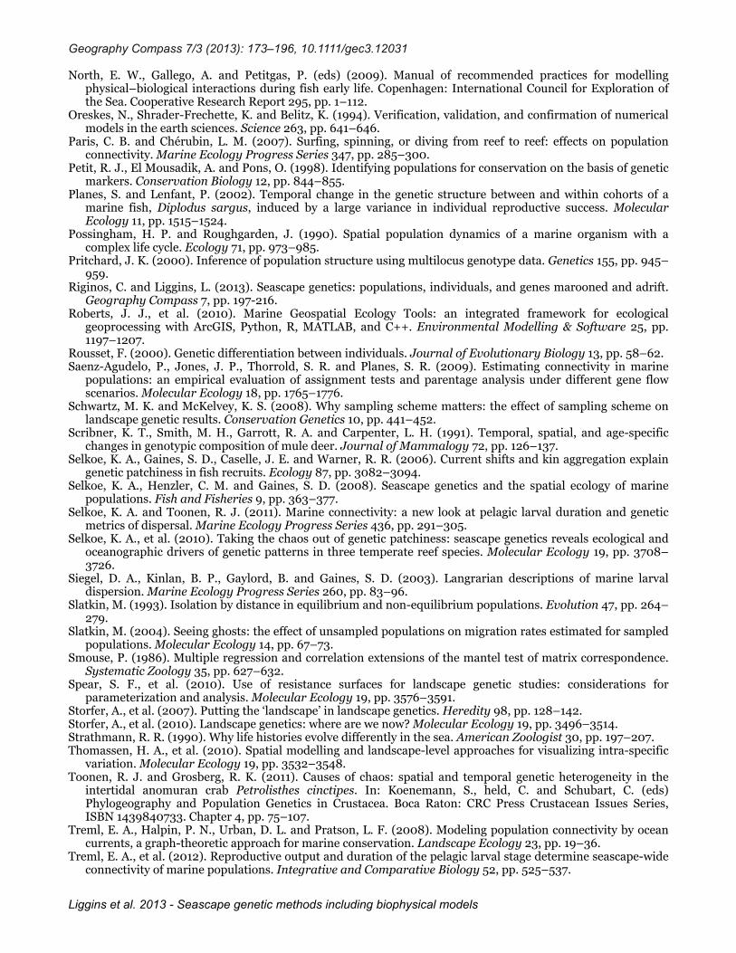
North, E. W., Gallego, A. and Petitgas, P. (eds) (2009). Manual of recommended practices for modelling physical–biological interactions during fish early life. Copenhagen: International Council for Exploration of the Sea. Cooperative Research Report 295, pp. 1–112.

Oreskes, N., Shrader-Frechette, K. and Belitz, K. (1994). Verification, validation, and confirmation of numerical models in the earth sciences. Science 263, pp. 641–646.

Paris, C. B. and Chérubin, L. M. (2007). Surfing, spinning, or diving from reef to reef: effects on population connectivity. Marine Ecology Progress Series 347, pp. 285–300.

Petit, R. J., El Mousadik, A. and Pons, O. (1998). Identifying populations for conservation on the basis of genetic markers. Conservation Biology 12, pp. 844–855.

Planes, S. and Lenfant, P. (2002). Temporal change in the genetic structure between and within cohorts of a marine fish, Diplodus sargus, induced by a large variance in individual reproductive success. Molecular Ecology 11, pp. 1515–1524.

Possingham, H. P. and Roughgarden, J. (1990). Spatial population dynamics of a marine organism with a complex life cycle. Ecology 71, pp. 973–985.

Pritchard, J. K. (2000). Inference of population structure using multilocus genotype data. Genetics 155, pp. 945–959.

Riginos, C. and Liggins, L. (2013). Seascape genetics: populations, individuals, and genes marooned and adrift. Geography Compass 7, pp. 197-216.

Roberts, J. J., et al. (2010). Marine Geospatial Ecology Tools: an integrated framework for ecological geoprocessing with ArcGIS, Python, R, MATLAB, and C++. Environmental Modelling & Software 25, pp. 1197–1207.

Rousset, F. (2000). Genetic differentiation between individuals. Journal of Evolutionary Biology 13, pp. 58–62. Saenz-Agudelo, P., Jones, J. P., Thorrold, S. R. and Planes, S. R. (2009). Estimating connectivity in marine

populations: an empirical evaluation of assignment tests and parentage analysis under different gene flow scenarios. Molecular Ecology 18, pp. 1765–1776.

Schwartz, M. K. and McKelvey, K. S. (2008). Why sampling scheme matters: the effect of sampling scheme on landscape genetic results. Conservation Genetics 10, pp. 441–452.

Scribner, K. T., Smith, M. H., Garrott, R. A. and Carpenter, L. H. (1991). Temporal, spatial, and age-specific changes in genotypic composition of mule deer. Journal of Mammalogy 72, pp. 126–137.

Selkoe, K. A., Gaines, S. D., Caselle, J. E. and Warner, R. R. (2006). Current shifts and kin aggregation explain genetic patchiness in fish recruits. Ecology 87, pp. 3082–3094.

Selkoe, K. A., Henzler, C. M. and Gaines, S. D. (2008). Seascape genetics and the spatial ecology of marine populations. Fish and Fisheries 9, pp. 363–377.

Selkoe, K. A. and Toonen, R. J. (2011). Marine connectivity: a new look at pelagic larval duration and genetic metrics of dispersal. Marine Ecology Progress Series 436, pp. 291–305.

Selkoe, K. A., et al. (2010). Taking the chaos out of genetic patchiness: seascape genetics reveals ecological and oceanographic drivers of genetic patterns in three temperate reef species. Molecular Ecology 19, pp. 3708–3726.

Siegel, D. A., Kinlan, B. P., Gaylord, B. and Gaines, S. D. (2003). Langrarian descriptions of marine larval dispersion. Marine Ecology Progress Series 260, pp. 83–96.

Slatkin, M. (1993). Isolation by distance in equilibrium and non-equilibrium populations. Evolution 47, pp. 264–279.

Slatkin, M. (2004). Seeing ghosts: the effect of unsampled populations on migration rates estimated for sampled populations. Molecular Ecology 14, pp. 67–73.

Smouse, P. (1986). Multiple regression and correlation extensions of the mantel test of matrix correspondence. Systematic Zoology 35, pp. 627–632.

Spear, S. F., et al. (2010). Use of resistance surfaces for landscape genetic studies: considerations for parameterization and analysis. Molecular Ecology 19, pp. 3576–3591.

Storfer, A., et al. (2007). Putting the ‘landscape’ in landscape genetics. Heredity 98, pp. 128–142.Storfer, A., et al. (2010). Landscape genetics: where are we now? Molecular Ecology 19, pp. 3496–3514. Strathmann, R. R. (1990). Why life histories evolve differently in the sea. American Zoologist 30, pp. 197–207. Thomassen, H. A., et al. (2010). Spatial modelling and landscape-level approaches for visualizing intra-specific

variation. Molecular Ecology 19, pp. 3532–3548. Toonen, R. J. and Grosberg, R. K. (2011). Causes of chaos: spatial and temporal genetic heterogeneity in the

intertidal anomuran crab Petrolisthes cinctipes. In: Koenemann, S., held, C. and Schubart, C. (eds) Phylogeography and Population Genetics in Crustacea. Boca Raton: CRC Press Crustacean Issues Series, ISBN 1439840733. Chapter 4, pp. 75–107.

Treml, E. A., Halpin, P. N., Urban, D. L. and Pratson, L. F. (2008). Modeling population connectivity by ocean currents, a graph-theoretic approach for marine conservation. Landscape Ecology 23, pp. 19–36.

Treml, E. A., et al. (2012). Reproductive output and duration of the pelagic larval stage determine seascape-wide connectivity of marine populations. Integrative and Comparative Biology 52, pp. 525–537.



Urban, D. L., Minor, E. S., Treml, E. A. and Schick, R. S. (2009). Graph models of habitat mosaics. Ecology Letters 12, pp. 260–273.

Waples, R. S. (1998). Separating the wheat from the chaff: patterns of genetic differentiation in high gene flow species. The Journal of Heredity 89, pp. 438–450.

White, C., et al. (2010). Ocean currents help explain population genetic structure. Proceedings of the Royal Society of London: Series B 277, pp. 1685–1694.

Whitlock, M. C. and McCauley, D. E. (1999). Indirect measures of gene flow and migration: FST ≠ 1 ⁄(4Nm+1). Heredity 82, 11, pp. 7–125.

Wright, S. (1931). Evolution in mendelian populations. Genetics 16, pp. 97–159. Wright, S. (1943). Isolation by distance. Genetics 28, pp. 114–138.



taking the plunge: an introduction to undertaking seascape

Documents