Electronic copy available at: http://ssrn.com/abstract=2777657

Tail protection for long investors: Convexity at work

J.-P. Bouchaud, T.-L. Dao, C. Deremble, Y. Lempérière, T.-T. Nguyen, M. Potters

May 9, 2016

Abstract

We relate the performance of trend following strategy to the di�erence between a long-term anda short-term variance. We show that this result is rather general, and holds for various de�nitionsof the trend. We use this result to explain the positive convexity property of CTA performance andshow that it is a much stronger e�ect than initially thought. This result also enable us to highlightinteresting connections with Risk Parity portfolio.

Finally, we propose a new portfolio of options that gives us a pure exposure to the variance ofthe underlying, shedding some light on the link between trend and volatility, and also helping usunderstanding the exact role of hedging.

1

Electronic copy available at: http://ssrn.com/abstract=2777657

Contents

1 Introduction 3

2 The trend on a single asset 5

2.1 A toy model for the trend . . . . . . . . . . . . . . . . . . . . . . . . . . . . . . . . . . 52.2 Trend following using an exponential moving average . . . . . . . . . . . . . . . . . . . 62.3 Changing the shape of the signal . . . . . . . . . . . . . . . . . . . . . . . . . . . . . . 62.4 A word on skewness . . . . . . . . . . . . . . . . . . . . . . . . . . . . . . . . . . . . . 72.5 Discussion . . . . . . . . . . . . . . . . . . . . . . . . . . . . . . . . . . . . . . . . . . . 7

3 Convexity at work on real data 8

3.1 Understanding the SG CTA Index . . . . . . . . . . . . . . . . . . . . . . . . . . . . . 83.1.1 The pool . . . . . . . . . . . . . . . . . . . . . . . . . . . . . . . . . . . . . . . 83.1.2 Comparing the performances with the SG CTA Index . . . . . . . . . . . . . . 83.1.3 The convexity of the SG CTA Index with the stock market . . . . . . . . . . . 9

3.2 Convexity and diversi�cation . . . . . . . . . . . . . . . . . . . . . . . . . . . . . . . . 103.2.1 Estimating the convexity of a diversi�ed trend with respect to the stock market 103.2.2 A global portfolio . . . . . . . . . . . . . . . . . . . . . . . . . . . . . . . . . . . 113.2.3 Reproducing a Risk-Parity index . . . . . . . . . . . . . . . . . . . . . . . . . . 113.2.4 Link between Trend and Risk Parity . . . . . . . . . . . . . . . . . . . . . . . . 12

4 The link with options 12

4.1 A collection of strangles . . . . . . . . . . . . . . . . . . . . . . . . . . . . . . . . . . . 134.2 Trend and re-hedging . . . . . . . . . . . . . . . . . . . . . . . . . . . . . . . . . . . . . 144.3 Conclusions . . . . . . . . . . . . . . . . . . . . . . . . . . . . . . . . . . . . . . . . . . 14

5 Summary and perspectives 15

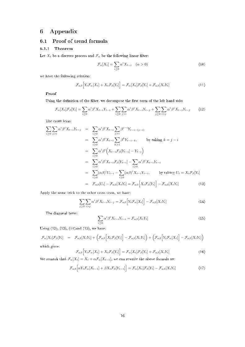
6 Appendix 16

6.1 Proof of trend formula . . . . . . . . . . . . . . . . . . . . . . . . . . . . . . . . . . . . 166.1.1 Theorem . . . . . . . . . . . . . . . . . . . . . . . . . . . . . . . . . . . . . . . 166.1.2 Discrete equation for EMA �lter . . . . . . . . . . . . . . . . . . . . . . . . . . 17

6.2 Generalized trend formula for trend-following . . . . . . . . . . . . . . . . . . . . . . . 176.2.1 Trend formula in continuous-time framework . . . . . . . . . . . . . . . . . . . 176.2.2 Linear trend estimation . . . . . . . . . . . . . . . . . . . . . . . . . . . . . . . 186.2.3 Non-linear trend estimation . . . . . . . . . . . . . . . . . . . . . . . . . . . . . 18

6.3 E�ect of diversi�cation . . . . . . . . . . . . . . . . . . . . . . . . . . . . . . . . . . . . 186.3.1 Convexity versus index . . . . . . . . . . . . . . . . . . . . . . . . . . . . . . . . 186.3.2 Convexity versus risk parity . . . . . . . . . . . . . . . . . . . . . . . . . . . . . 19

6.4 Strangle portfolio: Mark-to-the-market and Greeks . . . . . . . . . . . . . . . . . . . . 19

2

1 Introduction

A key concept in �nance is the idea of diversi�cation: if you can �nd decorrelated alphas, your totalperformance will be smoother, and your Sharpe ratio higher (see [9] for the original paper). Evenbetter is the situation when one strategy registers large gains on average when others take a hit(negative correlation). In particular, since a lot of investors have a long stock exposure, a strategythat performs well (or at least does not turn south) when the market goes down sounds like a veryuseful diversi�cation, and should be actively seeked by long investors.

A typical example of such a strategy is a long-option portfolio. Speci�c option portfolios, calledvariance swaps, are designed to give one an exposure to the realized variance of an asset, thereforeproviding direct protection when the volatility rises (see for example [20, 21] for detailed reviews onthe topic). Unfortunately, these portfolio typically exhibit strong negative drifts, which makes thema costly protection indeed.

Hedge funds are yet another alternative. The hedge fund industry has always claimed that itsperformance is not correlated to the market, and therefore hedge funds should be viewed as a sourceof diversi�cation, as well as providing pure alpha. However, if we plot the monthly performance ofthe HFRX index, a global Hedge Fund index, as a function of market return, like we do in �g.1, wesee a strong positive correlation between the two variables (i.e. when the market goes down, so dohedge funds returns), and a negative convexity: the performance is worse in periods of high marketvolatility, so that if we try a quadratic �t, the leading coe�cent is negative. In other words, hedgefunds seem to have di�culty ful�lling their promises in terms of diversi�cation (see [3] for a detailedanalysis of hedge fund performance).

One interesting exception to this is the case of CTAs: in 2008 in particular, their performanceduring the Lehman crisis was very strong, triggering a subsequent massive rise in assets (currentestimates are in the range of USD 300 bns, see [12]). This has been con�rmed by various studieswho have looked at CTA performance during or immediately after market crashes, and found aboveaverage performances [5, 10] (followed by below-par results, see [11] and references therein). Wereproduce the basis of these conclusions in �g.2 and 3, where we plot monthly returns of the twomain CTA indices as a function of market performance. As we can see, these strategies have indeedperformed on average better when the market volatility has been high.

Unfortunately, this convexity is based on �imsy statistical evidence (see [4] though), as quanti�edby the very low value of the R2 in both �ts (around 0.02). Therefore, it seems crucial to makesure that we are not looking at a statistical artifact. We will try in this paper to understand themechanism at work behind this convex behaviour, and to �nd a better way to quantify it, so thatwe can be assured this is not a statistical �uke (which we con�rm in �g.9). To do this, we will needto understand the trading patterns by CTAs, and the strategies they use.

As already noticed [3] (and we will demonstrate it again in this paper), CTA performance canactually be explained by one very simple strategy: trend following [13]. This strategy's robustnessand stability to a wide range of parameters, as well as the fact that it works across a large set of assetclasses, make the out-of-sample performance even more impressive, while the simplicity of the ideamakes it very suitable to the algorithmic trading style favoured by many CTA funds [14]. In a previouspaper, we have already studied the signi�cance of this strategy, and found that it is persistent over2 centuries [16], making it one of the most signi�cant market anomalies ever documented (barringsome HF e�ect). The problem we therefore want to tackle now is to understand, and quantify, theconvexity inherent to any trend following strategy.

We start by deriving some equations relating the performance of a single-asset trending strategyto the di�erence between a long-term and a short-term variance. We show that this result is rathergeneral, and holds for various de�nitions of the trend. We can then prove that this single-assettrend shows the expected convexity properties. To understand the CTA performance, we replicatethe SG CTA Index, using surprisingly few parameters. We can then understand how to measurethe convexity, and we will see a much stronger e�ect than naively plotted in �g.2. We will theninvestigate in detail the impact of diversi�cation on this convexity, and �nd interesting connectionswith Risk Parity strategies. Finally, we look at the most simple convex strategy: buying options. Weconsider a new portfolio of options that gives us a pure exposure to the variance of the underlying.We �nd that the pay-o� of these simpli�ed variance swaps appears to be strikingly similar to that ofa simple trending strategy. This shed some light on the link between trend and volatility, somewhatjustifying the "long vol" attribute of trend strategies, but also helps us understand the di�erencesbetween long-option portfolios and trending, and the exact role of hedging.

3

-10 %

-5 %

0 %

5 %

10 %

-20 % -15 % -10 % -5 % 0 % 5 % 10 % 15 % 20 %

Figure 1: Monthly returns of HFRI index vs. monthly returns of S&P. We see a concave relationship:hedge funds do worse when volatility is high.

-10 %

-5 %

0 %

5 %

10 %

-20 % -15 % -10 % -5 % 0 % 5 % 10 % 15 % 20 %

Figure 2: Monthly returns of BTOP 50 vs. monthly returns of S&P. We �t this with the ansatzy = ax2 + bx+ c. R2 = 0.02. The convexity is visible, but the R2 is low.

-10 %

-5 %

0 %

5 %

10 %

-20 % -15 % -10 % -5 % 0 % 5 % 10 % 15 % 20 %

Figure 3: Monthly returns of SG CTA Index vs. monthly returns of S&P. We �t this with the ansatzy = ax2 + bx+ c and get a convex function (R2 = 0.02).

4

2 The trend on a single asset

2.1 A toy model for the trend

We begin this study with a simpli�ed model, which will make all the derivations very straightforward,while keeping the main features of the more sophisticated models. We consider a predictor on day twhose value is simply the price di�erence between t and 0:

Pt = St − S0 =

tXi=0

∆i

where St is the price of our asset at day t, and ∆t = St − St−1 is the price di�erence (or return)between days t− 1 and t.

The daily P&L from t− 1 to t will be:

Gt = ∆tPt−1 = ∆t

t−1Xi=1

∆i

G1 = 0

Now we can aggregate the performance of our trending predictor from day 0 to a given day τ ,and re-arrange the sums:

τXt=2

Gt =

τXt=2

∆t

t−1Xi=1

∆i

=X

2≤t≤τ,i<t

∆t∆i

2

τXt=1

Gt =

τXt=1

∆t

!2

−τXt=1

∆2t

= (Sτ − S0)2 −τXt=1

∆2t

This simple formula is at the core of our understanding of the performance of a trending system.In a nutshell, it says that the performance, aggregated over τ days, is proportional to the di�erencebetween the realized variance computed over τ -days and the variance computed using 1-day returns.It makes perfect sense, since the di�erence between these 2 terms is the sum of cross-terms ∆t∆t′ ,which are related to the auto-correlation of the return. So the trend performance is positive if returnsare auto-correlated, which is very intuitive.

This calls for two more comments. First, we considered our time unit to be a day, but really, it isthe time over which we change our predictor, and rebalance our portfolio: this formula applies to afast, intraday trend as well as a monthly trend. We simply need to compute the short-term varianceover 1 time step, whatever that time step is.

Secondly, we have considered here ∆t to be price di�erences. Following simple optimizationprocedures to manage the heteroskedasticity of �nancial time series, it is quite customary to normalizethese returns by an estimate of the volatility, to have objects with unit variance (or as close to thatas possible). A typical example is some past exponential moving average of realized volatility overtime-scale τ :

σt = αqLτσ [∆2

t ]

with Lτ [Xt] = (1−λ)Pi≤t λ

t−iXi, and λ = 2τ+1

. α is an empirical factor that takes into account thefat tails of the return distribution, as well as the correlation of volatility. In practice, we consideredα = 1.05 and τσ = 10 in the rest of this paper.

We can reproduce all the computations above with normalized returns Rt = ∆tσt−1

, and �nd that

the performance of this new, risk-managed trend aggregated over τ days is:

τXt=1

Gt =1

2

τXt=0

Rt

!2

−τXt=0

R2t

!

We notice that, by de�nition, < R2t >= 1 if our volatility estimator is un-biased so the last term of

the eqution is known on average. This means that the performance of this simple trend is simplygoverned by the long-term variance of the underlying.

5

-30 %

-20 %

-10 %

0 %

10 %

20 %

30 %

40 %

50 %

60 %

-3 -2 -1 0 1 2 3

Figure 4: Mτ ′ [G] as a function of P , the past trend, for a trending system on the S&P with τ = 180.

If we consider a long history of this strategy, and split it in sub-samples of size τ , we can plot theperformance aggregated over this time scale as a function of the (normalized) return of the underlyingover the same time scale. This return is precisely X = 1√

τ

Pti+τt=ti

Rt. We have already pointed outthat the second term in the formula above averages to 1, so we get the conditional expectation ofthe pnl:

〈G〉X =τ

2(X2 − 1)

This formula is very simple, and clearly shows that we should expect convexity from such a simplestrategy, but only over a certain time-scale: it should work well when the underlying asset hasexperienced large moves over the trending time horizon. On the other hand, it does clearly notprovide a protection for a massive movement that happens over 1 time step; any price "jump" is nothedged by a trending strategy, and its average performance should be null.

2.2 Trend following using an exponential moving average

In reality, most funds use moving averages to compute their trending signals [18]. Therefore, it isimportant to generalize and extend our formula above to these types of �lters. In this subsection, weconsider a very standard trend-following strategy, which uses the exponential moving average (EMA)�lter to de�ne its prediction Pt =

√τLτ [Rt] (the extra factor

√τ simply ensures that our predictor

has unit variance).De�ning τ ′ = τ

2+ 1

2τ, and Gt = Pt−1Rt, we can write (see Appendix 6.1.2 for the proof):

Lτ ′ [Gt] =

√τ

τ − 1

`P 2t − Lτ ′

ˆR2t

˜´(1)

As we can see, here as well, the performance, once averaged over a suitable period of time, canbe rewritten as a di�erence beween 2 variance-type expressions: the �rst based on the aggregatedpast return (i.e. the position of our trend following system), and the second based on the 1-dayreturns properly re-normalized. Rather than the average performance, we may want to considerMτ ′ [Gt] = τ ′Lτ ′ [Gt], which is closer to the aggregated performance over time τ ′. If our volatilityestimate is un-biased and ensures that the second variance stays close to 1, then we have

〈Mτ ′ [G]〉P =τ ′√τ

τ − 1

`P 2 − 1

´(2)

As an illustration of the validity of this formula, we have plotted in �g.4 the cumulated perfor-mance over τ ′ daysMτ ′ [Gt] = τ ′Lτ ′ [Gt] for τ = 180 of a trend strategy with target volatility around15%. As we can see, we get a very good agreement between the theoretical line and the realizedperformance. In particular, the convexity is quite visible in this set-up, while it would have beenutterly blurred had we looked at 1-day, or even 1-month, returns.

This sensitivity to the averaging time means that we need to estimate carefully the time-scaleCTAs use to de�ne their trend if we want to see any clear sign of convexity in the CTA performances.

2.3 Changing the shape of the signal

In practice, people use a wide range of �lters to capture the trend anomaly: square average insteadof exponential, Vertical-Horizontal Filters, Strength Indices, crossing of 2 price averages... We want

6

-40 %

-30 %

-20 %

-10 %

0 %

10 %

20 %

30 %

40 %

-3 -2 -1 0 1 2 3

Figure 5: Mτ ′ [G] as a function of P , the past trend, for a 180-day saturated trending system on theS&P. The V-shape is very strong.

to present here a case of particular interest: what happens if we simply take the sign of our signal,rather than scaling our positions with the strength of it? This is quite common in practice, since itprevents us from taking extreme positions on one single asset, and loose the bene�ts of diversi�cation.

We can show that, in this case, we can rewrite the performance in the following form (see 6.2.3):

〈Mτ [Gt]〉P =√τ

|P | −

r2

π

!. (3)

We have plotted in �g.5 the typical shape of the cumulated performance over τ days Mτ [G] as afunction of P , and here as well, we get the best performance when the market experiences largevolatility over the time scale used to compute the trend. Instead of a parabolic �t, however, we seea piece-wise linear pro�le.

Since even in this extreme regime, we get a convex behaviour, we believe that intermediate caseswhere our positions should interpolate between the parabola of eq.1 and the V-shaped curve weobtained here, while keeping the convex feature of the trend.

2.4 A word on skewness

Skewness has been proposed as a measure of risk when determining what is a risk premium (see[17] for a thourough discussion on the subject). It is usually assumed that the skewness of trendfollowing is positive (see [1, 7] , and [2] for a general framework). Here, we can see that this followsdirectly from eq.1, on long time-scales at least. Indeed, if we assume that the returns follow agaussian distribution, then so does Pt, which is a linear combination of gaussian returns. Finally, theaggregated P&L varies as the square of Pt, which means that it follows a χ2 distribution, which hasa known positive skewness. So we see that the aggregated P&L of a trend does structurally showpositive skewness.

On a daily time scale, this is more subtle. If the returns are well-behaved, and exhibit somelevel of auto-correlation (i.e. if the P&L of the trend is positive on average), then it should exhibitpositive skewness. This explains the measured skewness on daily time-scales, since trend followinghas been a winning strategy over the last decades. In the absence of auto-correlation, however, thereis no reason to measure a positive skewness, as was already pointed out in [1].

2.5 Discussion

We have seen that the performance of a trending strategy, once aggregated over a suitable timehorizon, can be rewritten as a di�erence between a long-term and a short-term variance. If weproperly risk-manage our portfolio, the short-term variance is on average constant, and therefore theP&L is directly linked to the square of the past long-term return. In other words, there is a strongconvexity on this single-asset strategy.

It is striking that this conclusion does not depend on the overall perforamce of the trend itself;we may assume returns to be perfectly decorrelated, and hence the trend to have vanishing expectedreturn. Nonetheless, there would be convexity if we aggregate returns on the proper time scale.

7

Gov. bonds Short rates Indices FX Commodities10Y U.S. Note Euribor S&P 500 EUR/USD WTI Crude Oil

Bund Eurodollar EuroStoxx 50 JPY/USD GoldLong Gilts Short Sterling FTSE 100 GBP/USD Copper

JGB Nikkei 225 AUD/USD SoybeanCHF/USD

Figure 6: Liquid futures per sector. This selection is stable across time, and does not vary for decades.

We have also established that this result does not depend on the exact shape of the �lter: wego from a parabola to a V-shaped function if we take the sign of the average return, but the idearemains the same.

It is also interesting to recall that we are limited by the re-balancing period of the trend: if wetake an N-day trend, re-computed every n days, we can expect some protection when the marketmoves a lot over N days, but there is no such thing if there is a large sudden movement on a periodof time smaller than n days; our system is just blind to these oscillations. We need a quicker trendto take these into account.

3 Convexity at work on real data

In this section, we want to understand how our model is related to real data based on CTA per-formance. In particular, we conside the SG CTA Index 1, and show that our simple trend allow usto reproduce its performance (as previously shown in [13]). We �nd that the convexity we measureonce we get the right time scale, thoguh much larger than what we measure in the introduction (see�g.3), is not as high as what we observed in the previous section. This is of course because of thediversi�cation of contracts over which CTAs operate. Therefore, we will link the convexity of thediversi�ed trend with the performance of a diversi�ed long portfolio, whch we �nd to be very closeto that of a Risk Parity index.

3.1 Understanding the SG CTA Index

3.1.1 The pool

We �rst want to compare the performance of a simple trend following system to that of the mostfamous CTA index: the SG CTA Index. For simplicity, we considered in our simulations onlyfutures contracts in 5 sectors: stock indices, government bonds, short rates, foreign exchange, andcommodities. In each of these sectors, we considered the most liquid contracts. We end up with aselection outlined in table 6.

We believe that this selection is rather un-biased, since liquidity is quite stable over time, andthese contracts have been available for at least a few decades. In any case, adding or removing a fewcontracts should not a�ect our results.

3.1.2 Comparing the performances with the SG CTA Index

We have already de�ned a predictor Pt which has unit variance and is based over an EMA of thepast returns. We also have seen that we want a position on each asset which scales with the inverseof the volatility, so as to achieve a gain in percent Gkt on asset k with constant volatility (to �rstorder). We now want to be more speci�c: we de�ne Πk

t = P kt AL

σktto be the position a typical CTA

will take to follow predictor P kt on asset k. A is the assets under management of the fund, andL is its overall leverage ratio, used to achieve the relevant target volatility. These 2 quantities areconstant across time and assets. We also call wk the weight allocated to the strategy on asset k, sothat we can rewrite the total gain in percent as:

Gt =Xk

wkGkt =

Xk

wkΠkt−1∆k

t

A= L

Xk

wkPkt−1

∆kt

σkt−1

(4)

which is what we were looking for. We see that the total gain is the sum over all assets of terms withunit volatility, multiplied by the weight wk.

1Data available at the following URL: http://www.barclayhedge.com/research/indices/calyon/

8

0 %

20 %

40 %

60 %

80 %

100 %

0 50 100 150 200 250 300 350 400

Figure 7: correlation between Gt and the SG CTA Index as a function of the time-scale of the trend weused τ . As we can see, the maximum is around τ = 180 days.

0 %

20 %

40 %

60 %

80 %

100 %

120 %

140 %

2000 2002 2004 2006 2008 2010 2012 2014 2016

NewEdge CTA IndexReplicator

Figure 8: Cumulated returns of Gt and the SG CTA Index. We seem to capture all the alpha containedin the SG CTA Index with our simple replicator.

To compare our simulated performance Gt with the SG CTA Index, we need to determine thevalue of L, and determine the weights wk. Once again for the sake of simplicity, we choose toallocate the same amount of risk on each asset: wk = 1/N . We believe we could probably achieve ahigher correlation with a more sophisticated risk allocation (like in [15] for example), but we wantto keep this procedure as simple as possible, and, as we will see, this should be enough to allow us todetermine the time-scale of the trend used by CTAs. We then determine the value of L by requiringthat our simulated P&L should have the same volatility than the SG CTA Index. We �nd that weneed L = 0.01 no mater the time-scale of our trend, as long as P kt is properly normalized.

To be really accurate, and compare this strategy with traded funds, we need to make someassumptions on the fee structure. We assume a 1% �at fee for transaction costs ct, and a typical 2%management fee-20% incentive fee for the fund ft. We also took the 3-6 Month Treasury Bill indexas the risk-free rate rt, and de�ne Gt = Gt− ct− ft + rt as the total virtual performance of a typicalfund net of all fees and including capital gains.

To determine the relevant time scale, we can now compute Gt and correlate this with the SGCTA Index returns: Gt. The result of this procedure is plotted in �g.7. As we can see, there is amaximum in the correlation around τ = 180. This value is the typical time scale of the CTA trend.

What is actually striking is how high the correlation is (above 80%), while all we did was toperform a basic, un-sophisticated trend on the most liquid assets in the planet. Fig.8 shows thatwe actually capture most of the alpha contained in this index, since the Sharpe ratios of the twostrategies are very close. This shows that some of the alpha captured by CTAs can be understoodin terms of a very simple strategy.

3.1.3 The convexity of the SG CTA Index with the stock market

We have seen that we can reproduce quite accurately the performance of CTAs as measured by theSG CTA Index, using a simple trend with very few parameters. We only need one global multiplier

9

-10 %

-5 %

0 %

5 %

10 %

15 %

20 %

25 %

30 %

-3 -2 -1 0 1 2 3

Figure 9: Cumulated performance over τ ′ days of the SG CTA Index as a function of Pt on the S&Pfuture, with τ = 180. R2 = 0.18, which is quite better than what we have if we use monthly data (see�g.3).

L to ensure that our simulation has the right volatility, and we �t the time scale of the trend tomaximze the correlation. We �nd the optimal value τ = 180, and achieve a very good level ofcorrelation for such a crude simulation, above 80%. No doubt that we could improve that if we allowfor a more sophisticated portfolio allocation.

This is beyond the scope of this paper, however: we were merely looking for the best value forτ , which we �nd to be τ = 180, and τ ′ = 90. We can now see if the convexity is in any waymore apparent if we average like we propose in Eq.2. We therefore computeMτ ′ [Gt] = τ ′Lτ ′ [Gt],the cumulated SG CTA Index performance over τ ′ days, as a function of the S&P return over thetrending time scale τ : Pt =

√τLτ [Rt]. The result is plotted in �g.9, and as we can see, we do get a

much more convincing R2 (0.2 in stead of 0.02).So it does seem there is some convexity in the SG CTA Index, if we average our variables over

the right time scales. The still relatively low value of the R2 can intuitively be understood: it comesfrom the fact that we need more than one asset to reproduce the index, and therefore, we only havea noisy version of the single-asset convexity we studied in the previous section. We therefore needto understand how this diversi�cation will a�ect the convexity of a trending strategy.

3.2 Convexity and diversi�cation

We have seen in the previous section that the convexity of the SG CTA Index with respect to onesingle asset, though signi�cant, is far from perfect because of its diversi�cation. Therefore, we shouldestimate how this diversi�cation a�ects the relationship outlined in eq.2. To further understand whatportfolio a diversi�ed trend is actually hedging, we will introduce a long-only diversi�ed portfolio,and show that a diversi�ed trending strategy is convex with respect to this product. We �nally linkthis long-only portfolio to Risk Parity indices.

3.2.1 Estimating the convexity of a diversi�ed trend with respect to the stock

market

As explained above, convexity in the industry is often understood in terms of stock market returns:what does a strategy do if the stock market moves a lot, either up or down? That is perfectlyunderstandable since many investors are exposed to the stock market, and are therefore eager tohave a hedge in case of a market crash. We have seen before that a trending strategy on the indexitself provides a strong hedge, but this leads to rather poor performances. CTAs usually propose adiversi�ed strategy, which therefore dilutes the convexity.

We now want to quantify this. In Appendix 6.3, we show that, in a certain limit (negligibledrifts in all assets, correct normalization of returns...), we can rewrite the relationship between thecumulated return over τ ′ of a diversi�ed trend strategy and the past trend on the stock index as:

Mτ ′ [Gt] ∝ β2`P 2t − 1

´(5)

with Pt the trend on the index, and β2 =Pk β

2k the average of the squared β between each asset

and the stock market.

10

This result is rather intuitive: if the market moves a lot over τ ′, showing a high return auto-correlation, then an asset with either a very positive or a very negative β will show a similar amountof auto-correlation (i.e. strong performance for a trending strategy), so it makes sense to considerβ2k. Alternatively, when βk is close to 0, there is no reason to expect any hedge from this asset in

case of market turmoil.Eq.5 explains why our R2 is not higher in Fig.9: all asets are obviously not 100% correlated with

the S&P! Incidentally, the correlation we get betweenMτ ′ [Gt], the aggregated performance, and P 2t

on the S&P is a measure of the average β2 of our portfolio with the S&P. With the portfolio outlinedabove, and the value of our R2, we get β2 = 0.23, which seems consistent with the pool of assets weconsider.

3.2.2 A global portfolio

We now want to introduce a portfolio in which we have a long position on every asset that we usein our SG CTA Index replicator. Namely, we consider positions A L

σkt, where A represents the assets

under management, and L the leverage we use, so that the percentage returns of this portfolio canbe written as:

Grpt = LXk

wk∆kt

σkt−1

(6)

This portfolio is some sort of a global portfolio, being exposed to everything we have in our universe:indices, bonds, commodities, and a basket of currencies. We also note that the risk taken on everyasset is the same.

Now, to hedge this portfolio, we could use a trend following strategy on its own performance Grp:we go long when this portfolio has made money over the last τ days, and short otherwise. Thatwould lead to results very similar to the ones shown in Fig.4; namely, we would �nd a very strongconvexity.

We now want to show that the diversi�ed trend CTAs do also provides a hedge for this portfolio,that is actually better than just a trend on the global portfolio. To do so, and remembering that Gtis the P&L of the SG CTA Index replicator, we notice that:

〈Mτ ′ [Gt]〉P =Xk

wk〈Mτ ′ [Gkt ]〉kP =

Xk

wkLτ ′√τ

τ − 1((P kt )2 − 1) ≥ Lτ

′√ττ − 1

(P 2 − 1)

where P =Pk wkP

kt , and we used the convexity of the parabola in the �nal step of the derivation.

Using Eq.6, we can rewrite this in the form:

Mτ ′ [Gt] ≥τ ′√τ

τ − 1

`(Mτ [Grpt ])2 − 1

´(7)

Eq.7 shows how good the diversi�ed hedge performs: while a normal trend on the portfolioensures that the performance stays on average on the parabola, the diversi�cation means that weare on average above this parabola. This means that CTAs do provide a very signi�cant protectionto large moves in this global portfolio we have built. We now have to �nd out how we can interpretthis long-only portfolio.

3.2.3 Reproducing a Risk-Parity index

Risk-Parity is a class of investment that, like CTAs, takes positions in a wide range of securities. Themain feature of this strategy is, as emphasized by its name, the fact that each asset class provides thesame contribution to the global risk (Equal Risk Contribution, see [19] for an excellent introductionon the subject). To �rst order, assuming the asset cross-correlations all take the same value, it meansthat the positions on a given asset scales inversely with its volatility, just like our positions when wereproduce the SG CTA Index. In Risk-Parity, however, we only take long positions, which makes ita good candidate to understand our global portfolio.

Based on these similarities, we tried to compare our portfolio with J.P. Morgan Risk-Parity indexusing the same ideas than for the SG CTA Index. Here as well, we �t L in Eq.6 so that our simulationhas the same volatility than the real index, (we �nd L = 0.0114), and we use equal weighting amongstour pool. We also made assumptions for the costs: no execution costs (always long), and a 1% �atmangement fee. The risk-free rate is the same, so that we can also de�ne Grpt = Grpt − f

rpt + rt as

the performance of our global portfolio, net of all fees.Based on these assumptions, we are able to reproduce the J.P. Morgan Risk Parity index with

a very good precision (see �g.10): the correlation is as high as 89%! No doubt that here as well,

11

0 %

5 %

10 %

15 %

20 %

25 %

Jan 2011 Jan 2012 Jan 2013 Jan 2014 Jan 2015

JP Morgan Risk Parity IndexReplicator

Figure 10: Replication of the J.P. Morgan Risk-Parity index using our pool of futures. The correlationis strikingly high, at 89%, and we seem here as well to capture most of the alpha in the product.

-10 %

-5 %

0 %

5 %

10 %

15 %

20 %

25 %

30 %

-20 % -10 % 0 % 10 % 20 %

Figure 11: Cumulated CTA performanceM[G] as a function of the cumulated Risk-Parity performanceM[Grp]. We use our own proxies built on the pool in table 6

we could increase this level by choosing a more appropriate set of product weights through a moresophisticated portfolio construction, but we feel this is good enouh for our purposes, and it wouldnot a�ect our results anyway.

3.2.4 Link between Trend and Risk Parity

We can now understand the meaning of our global portfolio, that is actually very close to a RiskParity investment. therefore, Eq.7 tells us that a diversi�ed trend provides a very good hedge for aRisk Parity investor.

To con�rm this, we have used our proxies for CTA and Risk-Parity performance Gt and Grpt . In

�g.11, we plotMτ ′ [Gt] as a function ofMτ [Grpt ]. As we can see, the inequality is indeed satis�ed.We reproduced this experiment, using real data from the o�cial indices (we needed to put back thecosts to make the performances comparable, however, so we used the assumptions we made in theprevious section). We show the result in �g.12. In both cases, the inequality is very well satis�ed.What this means is that trend following does naturally provide a hedge to those investors exposed toRisk Parity. Indeed, as eq.7 shows, when Risk Parity experiences a large drawdown, we can expecta good performance from the trend.

4 The link with options

We now turn to another feature of trend following strategies: various papers have mentionned theirsimilarities with long-option portfolios, such as At-The-Money (ATM) straddles (a portfolio com-posed of a Put and a Call option both at the money). This is a very natural connection, sinceboth strategies have known convex properties. We want to link these results to our formalism. Wewill propose a new option portfolio that allow us to capture a long-volatility performance in a very

12

-10 %

-5 %

0 %

5 %

10 %

15 %

20 %

25 %

30 %

-20 % -10 % 0 % 10 % 20 %

Figure 12: Cumulated SG CTA Index performance M[G] as a function of the cumulated J.P. MorganRisk-Parity index performanceM[Grp]. We put back costs to create "pure" performances.

simple, model-free way (that does not require any black-Scholes inspired machinery). The pay-o� ofthis portfolio is actually very close to that of a trend following strategy. We will see how a trendingstrategy is very naturally interpreted as the hedge of this portfolio, and how this hedge essentiallyswaps the long-term variance for the short-term one. It also gives us a more detailed understandingof the volatility we are exposed to in each case, and why the price we pay for the protection isdi�erent.

4.1 A collection of strangles

We begin our study by considering a simple straddle, composed of an ATM Put and an ATM Calloption (similar to what was considered in [23]). It is quite straightforward to verify that the pay-o�of this portfolio can be written as:

G[0,T ] = |ST − S0| − (CS0,T + PS0,T )

= |∆[0,T ]| −r

2

πS0

√Tσatm,T

where σatm is the ATM implied volatility. We notice that we are exposed to the total return between0 and T . To get an expression which looks closer to eq.1, we need to consider an in�nite equi-weightedcollection of strangles, centered at the money:

Uniform pro�le = 2

Z S0

0

(K − ST )+dK| {z }h(S0−ST )+

i2+ 2

Z ∞S0

(ST −K)+dK| {z }h(ST−S0)+

i2= (ST − S0)2

After a simple integration, we can see that this portfolio has the following pay-o�:

PnlStrangles[0,T ] =1

2

`∆2

[0,T ] − T σ2´ (8)

where σ is de�ned by:

σ =

s2

T

` Z S0

0

PK,T +

Z ∞S0

CK,T´

Eq.8 is quite suggestive. It tells us that this portfolio receives the long-term variance ∆2[0,T ], and

pays a �xed price at the start of the trade: σ2. Note that this long-term variance is the same wereceive when we follow our toy trend following model at the start of this paper. The only di�erence isthe price we pay to receive this variance: realized vs. implied volatility. Since options are notoriouslysold at a premium, an option strategy would be more expensive than a trend following one.

In practice, we can only buy a �nite set of options, but, just like any trend strategy shouldinterpolate between the linear and the fully capped trend (Eq. 1 and 5), we believe that the pay-o�of our real portfolio should lie somewhere in between the pay-o� of our in�nite collection of strangles,and that of a single straddle. The farther we can go, the larger the quadratic region will be.

13

Figure 13: Re-balancing uniform-weight portfolio by trading futures between two spot prices

4.2 Trend and re-hedging

At t = 0, our option portfolio satis�es ∆ = 0, since we consider strangles centered at the money.We can try intuitively to understand what is the hedging trade we have to do when the spot pricemoves from S0 to St. Figuratively, we have to re-center our portfolio P around the new price St, sowe have to exchange Calls for Puts (Puts for Calls) if the price has gone up (down) between St andS0. But selling a Call and buying a Put at the same strike is the same as selling the underlying, sothe hedging tells us to sell the underlying, by an amount St−S0 when the price goes up, and to buyit if it goes down (see �g.13 for an illustration of this procedure).

This trade hedge is exactly the opposite of what our toy-model for trend following does, so weknow the hedge performance can be written as:

Pnlhedge = −(∆2[0,T ] −

Xt

∆2t )

We derive in Appendix 6.4 formulae for all the usual greeks in a more mathematical way, but itis quite neat to see that we can get a feeling for ∆ that is accurate.

If we add the pay-o� of our portfolio with this re-hedge performance, we get the total performanceof our hedged portfolio of strangles:

PnlHedg.Str[0,T ] =Xt

∆2t − T σ2 (9)

4.3 Conclusions

As we can see, the hedging strategy exchanges the variance of the total return over the period [0, T ]with the variance de�ned using the re-hedging frequency (see[22] for a detailed account on the role ofhedging, and [24] for a derivation of the importance of the hedging frequency in a di�erent set-up).At the end, our portfolio exhibits the exact performance of a variance swap, but the formulae weused are model-independant, we never need Black-Scholes inspired models. This type of constructionalso helps us understand that it is the hedging strategy that decides which volatility we are exposedto: if we re-hedge every 5 minutes, we get the volatility of 5-minutes returns, while we get dailyvolatility if we re-hedge at the close of the day. The price we pay for the options σ, on the otherhand, is always the same.

It also helps us clarify the similarities between a trend following system and a long naked straddleportfolio. They are both exposed to the long term variance ∆2

[0,T ] (i.e. they both provide protectionfor a long-stock portfolio), but the second one buys that exposure at a �xed price σ while the �rstone pays the short-term variance

Pt ∆2

t . An interesting consequence is that, if a shock occurs in onesingle day that dominates the return over the interval [0, T ], the naked straddle will make money,since the entry price is �xed, while the trend will be �at on average. In other words, the straddle isa better hedge, and therefore its price σ should be higher than the real volatility

Pt ∆2

t .The premium we pay on options is however quite high, and long-gamma portfolios have been

consistently losing money over the past 2 decades, while trend following has actually posted positiveperformance. So, even if options provide a better hedge, it still seems that trend following is a muchcheaper way to hedge a long-only exposure.

14

5 Summary and perspectives

In this paper, we have shown that a single-asset trend has a built-in convexity if we aggregate itsreturns over the right time-scale. This becomes apparent if we rewrite the performance of the trend asa swap between the variance de�ned over long-term returns (typically the time scale of the trending�lter) and the one de�ned over short-term returns (the rebalancing of our portfolio). This featureappears to hold for various �lters and saturation levels.

The importance of these 2 time-scales has been underlined, and it is clear that the convexity (andthe hedging propoerties) are only present over long-term time scales (as de�ned by the trending �lteritself): it is wrong to expect a 6-month trending system rebalanced every week to hedge against amarket crash that lasted only a few days.

We also turned our attention to CTA indices, and particularly the SG CTA Index. We haveproposed a simple replication index, using a very natural un-saturated trend on a pool of very liquidassets. Assuming realistic fees, and �tting only the time-scale of the �lter, we get a very goodcorrelation (above 80%), and capture the drift completely. This shows again that CTAs are simplyfollowing a long-term trending signal, and there is little added value in their idiosyncrasies.

However, this also shows us that a CTA does not provide the same hedge a single-asset trendprovides: some of the convexity is lost because of diversi�cation. We however have found thatCTAs do o�er an interesting hedge to Risk-Parity products, which we approximated with a verygood precision by long positions on the main asset classes. This property is quite new, and we feelit makes the trend a valid addition in the book of any manager holding Risk Parity products (orsimply a diversi�ed long position in both equities and bonds).

We then turned our attention to the link between trend and volatility. We found that a simpletrending toy-model shares an exposure to the long-term variance with a naked straddle. The dif-ference is the fact that the entry price for the straddle is �xed by the at-the-money volatility, whilethe trend pays the realized short-term variance. We then propose a very clean way to get exposureto this short term variance by using the trending toy-model as a hedging strategy for a portfolio ofstrangles. This is a simple, model-free portfolio that o�ers the same pay-o� than traditional varianceswaps.

All in all, these results prove that a trending system does o�er protection to long-term largemoves of the market. This, coupled with the high signi�cance of this market anomaly, really setsit apart in the world of investment strategies. A more pressing issue could be the capacity of thisstrategy, but recent performance seems to be quite in line with long-term returns, so there is littleevidence of over-crowding.

The future of CTA industry is still unclear, whether large established funds will continue tocharge thier usual fees, or if cheaper investment vehicles will attract interest. What we have seen inthis paper is that there is little value in the "superior skill" of a single CTA, unless this CTA hascorrelation with the SG CTA Index that is signi�cantly below 80% (i.e. it does something di�erentfrom what we have proposed). For a simple trend exposure (which is desirable in a diversi�edportfolio), a cheap alternative may well be enough.

15

6 Appendix

6.1 Proof of trend formula

6.1.1 Theorem

Let Xt be a discrete process and Fα be the following linear �lter:

Fα[Xt] =Xi≥0

αiXt−i (α > 0) (10)

we have the following relation:

FαβhYtFα[Xt] +XtFβ [Yt]

i= Fα[Xt]Fβ [Yt] + Fαβ [XtYt] (11)

Proof

Using the de�nition of the �lter, we decompose the �rst term of the left hand-side:

Fα[Xt]Fβ [Yt] =Xi≥0

αiβiXt−iYt−i +Xi≥0

Xj>i

αiβjXt−iYt−j +Xj≥0

Xi>j

αiβjXt−iYt−j (12)

The cross term:Xi≥0

Xj>i

αiβjXt−iYt−j =Xi≥0

αiβiXt−iXj>i

βj−iYt−i−(j−i)

=Xi≥0

αiβiXt−iXk≥1

βkYt−i−k, by taking k = j − i

=Xi≥0

αiβi“Xt−iFβ [Yt−i]− Yt−i

”=

Xi≥0

αiβiXt−iFβ [Yt−i]−Xi≥0

αiβiXt−iYt−i

=Xi≥0

(αβ)iUt−i −Xi≥0

(αβ)iXt−iYt−i, by taking Ut = XtFβ [Yt]

= Fαβ [Ut]−Fαβ [XtYt] = FαβhXtFβ [Yt]

i−Fαβ [XtYt] (13)

Apply the same trick to the other cross term, we have:Xj≥0

Xi>j

αiβjXt−iYt−j = FαβhYtFα[Xt]

i−Fαβ [XtYt] (14)

The diagonal term: Xi≥0

αiβiXt−iYt−i = Fαβ [XtYt] (15)

Using (12), (13), (14)and (15), we have:

Fα[Xt]Fβ [Yt] = Fαβ [XtYt] +“Fαβ

hXtFβ [Yt]

i−Fαβ [XtYt]

”+“Fαβ

hYtFα[Xt]

i−Fαβ [XtYt]

”which gives:

FαβhYtFα[Xt] +XtFβ [Yt]

i= Fα[Xt]Fβ [Yt] + Fαβ [XtYt] (16)

We remark that Fα[Xt] = Xt + αFα[Xt−1], we can rewrite the above formula as:

FαβhαYtFα[Xt−1] + βXtFβ [Yt−1]

i= Fα[Xt]Fβ [Yt]−Fαβ [XtYt] (17)

16

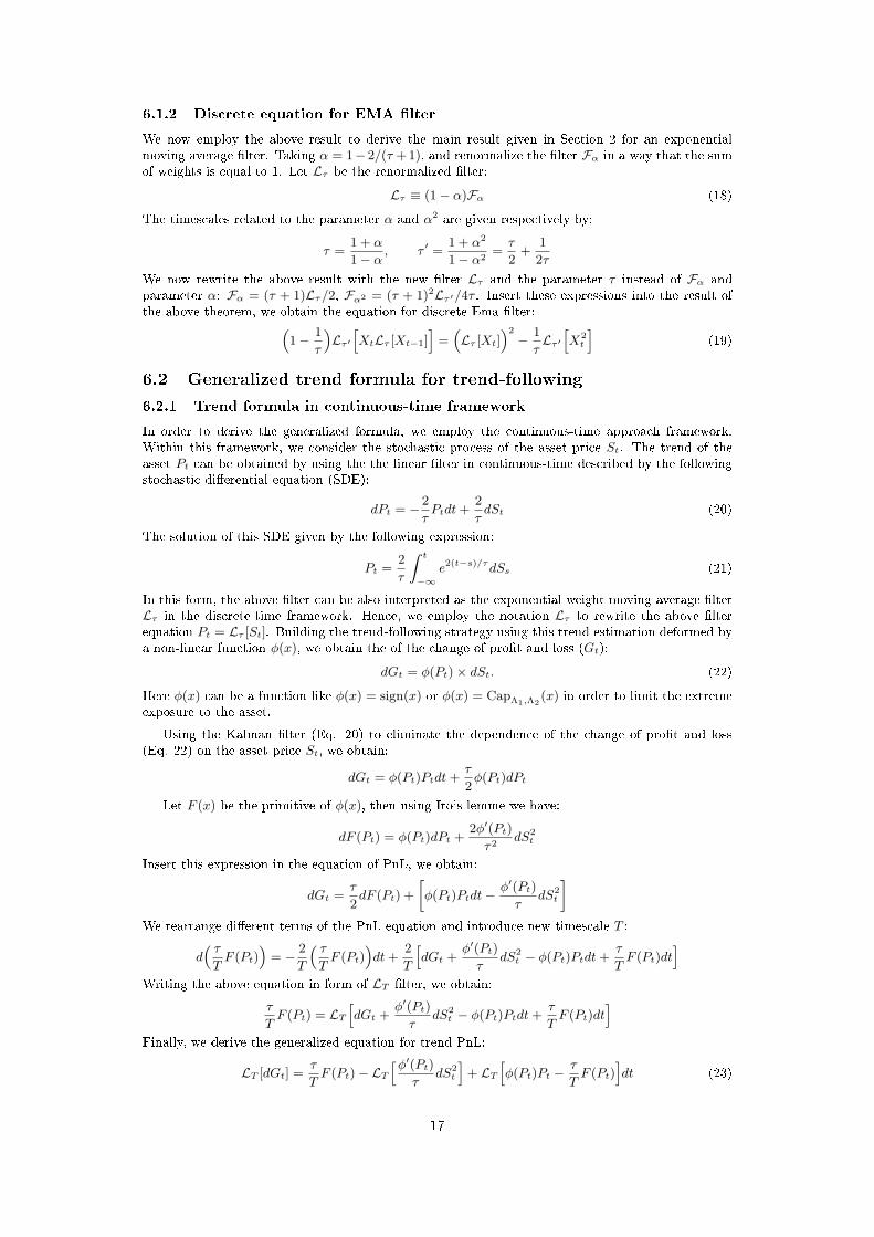
6.1.2 Discrete equation for EMA �lter

We now employ the above result to derive the main result given in Section 2 for an exponentialmoving average �lter. Taking α = 1− 2/(τ + 1), and renormalize the �lter Fα in a way that the sumof weights is equal to 1. Let Lτ be the renormalized �lter:

Lτ ≡ (1− α)Fα (18)

The timescales related to the parameter α and α2 are given respectively by:

τ =1 + α

1− α, τ ′ =1 + α2

1− α2=τ

2+

1

2τ

We now rewrite the above result with the new �lter Lτ and the parameter τ instead of Fα andparameter α: Fα = (τ + 1)Lτ/2, Fα2 = (τ + 1)2Lτ ′/4τ . Insert these expressions into the result ofthe above theorem, we obtain the equation for discrete Ema �lter:“

1− 1

τ

”Lτ ′hXtLτ [Xt−1]

i=“Lτ [Xt]

”2

− 1

τLτ ′hX2t

i(19)

6.2 Generalized trend formula for trend-following

6.2.1 Trend formula in continuous-time framework

In order to derive the generalized formula, we employ the continuous-time approach framework.Within this framework, we consider the stochastic process of the asset price St. The trend of theasset Pt can be obtained by using the the linear �lter in continuous-time described by the followingstochastic di�erential equation (SDE):

dPt = − 2

τPtdt+

2

τdSt (20)

The solution of this SDE given by the following expression:

Pt =2

τ

Z t

−∞e2(t−s)/τdSs (21)

In this form, the above �lter can be also interpreted as the exponential weight moving average �lterLτ in the discrete-time framework. Hence, we employ the notation Lτ to rewrite the above �lterequation Pt = Lτ [St]. Building the trend-following strategy using this trend estimation deformed bya non-linear function φ(x), we obtain the of the change of pro�t and loss (Gt):

dGt = φ(Pt)× dSt. (22)

Here φ(x) can be a function like φ(x) = sign(x) or φ(x) = CapΛ1,Λ2(x) in order to limit the extreme

exposure to the asset.

Using the Kalman �lter (Eq. 20) to eliminate the dependence of the change of pro�t and loss(Eq. 22) on the asset price St, we obtain:

dGt = φ(Pt)Ptdt+τ

2φ(Pt)dPt

Let F (x) be the primitive of φ(x), then using Ito's lemme we have:

dF (Pt) = φ(Pt)dPt +2φ′(Pt)

τ2dS2

t

Insert this expression in the equation of PnL, we obtain:

dGt =τ

2dF (Pt) +

»φ(Pt)Ptdt−

φ′(Pt)

τdS2

t

–We rearrange di�erent terms of the PnL equation and introduce new timescale T :

d“ τTF (Pt)

”= − 2

T

“ τTF (Pt)

”dt+

2

T

hdGt +

φ′(Pt)

τdS2

t − φ(Pt)Ptdt+τ

TF (Pt)dt

iWriting the above equation in form of LT �lter, we obtain:

τ

TF (Pt) = LT

hdGt +

φ′(Pt)

τdS2

t − φ(Pt)Ptdt+τ

TF (Pt)dt

iFinally, we derive the generalized equation for trend PnL:

LT [dGt] =τ

TF (Pt)− LT

hφ′(Pt)τ

dS2t

i+ LT

hφ(Pt)Pt −

τ

TF (Pt)

idt (23)

17

6.2.2 Linear trend estimation

In the case where φ(x) = x, we have F (x) = x2/2, then we �nd the result showed for discreteapproach:

LT [dG] =τ

2TP 2t −

1

τLT [dS2

t ] +“

1− τ

2T

”LT [P 2

t ]dt (24)

With the choice of timescale T = τ/2 we eliminate the last term (correction term) then obtain:

LT [dG] = P 2t −

1

2TLT [dS2

t ] (25)

6.2.3 Non-linear trend estimation

Let us consider now the case φ(x) = sign(x) hence its primitive is F (x) = |x| and its derivative isφ′(x) = 2δ(x). We obtain:

LT [dGt] =τ

T|Pt| −

2

τLThδ(Pt)dS

2t

i+“

1− τ

T

”LT [|Pt|]dt

With the choice of timescale T = τ , we eliminate the last term (correction term) then obtain thefollowing equation:

Lτ [dGt] = |Pt| −2

τLτhδ(µt)dS

2t

iFor return dSt is risk managed at stable volatility σ and follows Gaussian process dSt ∼ N (µ, σ), wehave the following approximation: D

Lτhδ(Pt)dS

2t

iEP≈ σ2〈δ(P )〉

As the trend estimate Pt follows the following distribution N (µ, σ/√τ), we have:

〈δ(P )〉 =

Z ∞−∞

δ(x)1√

2πσµe−x

2/2σµdx =

rτ

2π

1

σ

Insert this approximation in the PnL equation, we obtain the result for the case of sign of trend:

〈Lτ [dGt]〉P = |Pt| −r

2

πτσ (26)

Renormalize the predictor as Pt → Pt√τ/σ, we obtain the formula:

〈Mτ [dGt]〉P =√τ“|Pt| −

r2

π

”(27)

6.3 E�ect of diversi�cation

We provide here the proofs of the convexity of the trend with respected to the index and the risk-parity portfolio for the multi-asset case.

6.3.1 Convexity versus index

Let us consider a multi-asset trend following portfolio with weight distribution {wk} for k = 1 . . . Nover N assets with return ∆k. We derive now convexity with respected to a given asset (S&P indexfor example) denoted by index s. Let us de�ne some notation:

Pk,t = Pk,t − αk with αk = E[Pk,t] and ν2k = E[P 2

k,t]

Therefore Ps,t is the trend estimated on the return of the asset s. We project now the individualtrend Pk,t on this direction and obtain:

Pk,t = βkPs,t + αk,t with βk =E[Pk,tPs,t]

ν2s

Insert this decomposition in the sum of individual trend formula and perform some algebraic calcu-lations, we obtain �nally: D

Mτ ′ [Gt] | Ps,t = pE→ lβ2

“p2 − ν2

s + α2”

18

in which the di�erent average quantities β2, α2, α, ν2s are de�ned as below:

β2 =1

N

NXk=1

β2k, α2 =

PNk=1 α

2kPN

k=1 β2k

, α =

PNk=1 βkαkPNk=1 β

2k

Ps,t = Ps,t + α, ν2s = E[P 2

s,t] = ν2s + α2

Note that if all drifts are zero in average and if the time series are properly normalized the aboveequation simply writes:

Mτ ′ˆGt˜≈ lβ2

`P 2s,t − 1

´(28)

6.3.2 Convexity versus risk parity

We can de�ne the total trend indicator:

Pt =

NXk=1

wkPk,t

Applying the trend formula for individual products then performing the weighted sum using {wk},we obtain:

Mτ ′ [Gt] ≥ l

P 2t −

NXk=1

wkLτ ′ [∆2k,t]

!Taking conditional expectation on the total trend, we obtain similar result for the single asset case:

˙Mτ ′ [Gt] | Pt = p

¸≥

*l

P 2t −

NXk=1

wkLτ ′ˆ∆2k,t

˜!| Pt = p

+→ l

`p2 − 1

´This result provides a lower bound of the convexity with respected the weighted average trend.

We now rewrite the above inequality in form of the �lter Mτ instead of the EMA-�lter Lτ forboth sides then obtain:

Mτ ′ [Gt] ≥ l„Mτ [Rt]

2

τ− 1

«(29)

6.4 Strangle portfolio: Mark-to-the-market and Greeks

In this appendix, we compute the mark-to-the-market PnL of the above payo�:

PnL[0,T ] = R2[0,T ] − T σ2

T

Here, σ2 is the implied variance of daily return.

σ2T =

2

T

“Z S0

PK,T +

ZS0

CK,T”

Let us employ the following decomposition at time t ∈ [0, T ]:

R2[0,T ] =

“R[0,t−1] +R[t,T ]

”2

= R2[0,t−1] + 2R[0,t]R[t,T ] +R2

[t,T ]

Pricing this quantity at time t by the market-measure E gives us the mark-to-the-market value ofthis payo�:

PnL[0,t] = Et“R2

[0,T ]

”− T σ2

T

= R2[0,t−1] +R[0,t−1]Et

“R[t,T ]

”+ Et

“R2

[t,T ]

”− T σ2

T

= R2[0,t−1] +R[0,t−1]Et

“ST − St

”+ Et

“R2

[t,T ]

”− T σ2

T

19

Here, we have to price a new portfolio of strangles Et“R2

[t,T ]

”centered at St and a future contract

Et“ST − St

”with fair price zero. The new strangles portfolio gives us simply τ σ2

τ while the fair

price of future contract is zero. Hence, we obtain �nally the market price of our original portfolio:

PnL[0,t] = R2[0,t−1] + τ σ2

τ − T σ2T

Here τ = T − t is the time-to-maturity. Therefore, the daily mark-to-the-market PnL is given by:

PnLt = PnL[0,t+1] − PnL[0,t]

= R2t + ((τ − 1)σ2

τ−1 − τ σ2τ ) + 2R[0,t−1]Rt

=“R2t − σ2

τ−1

”| {z }Gamma PnL

+ τ“σ2τ−1 − σ2

τ

”| {z }

Vega PnL

+ 2(St − S0)Rt| {z }Delta PnL

From the above equation, we deduce simply the global Greeks of the strangle portfolio:

Γ = 1, V = 2τ στ , ∆t = 2(St − S0) (30)

20

References

[1] Marc Potters, Jean-Philippe Bouchaud.: Trend followers lose more often than they gain, arxiv,(august 2005).

[2] Benjamin Bruder, Nicolas Gaussel: Risk-Return Analysis of Dynamical investment Strategies,Lyxor White Paper, Issue 7 (june 2011).

[3] Fung W. and Hsieh D.A.: Empirical Characteristics of Dynamic Trading Strategies: The Caseof Hedge Funds, Review of Financial studies, 10(2), pp. 275-302 (1997).

[4] Fung W. and Hsieh D.A.: Survivorship bias and Investment Style in the Returns of CTAs, Journalof Portfolio Managemenent, 23 (30-41)

[5] Fung W. and Hsieh D.A.: The Risk in Hedge Fund Strategies: Theory and Evidence from TrendFollowers, Review of Financial studies, Review of Financial studies, 14(2), pp. 313-341.

[6] Brian Hurst , Yao Hua Ool and Lasse H. Pedersen: A Century of Evidence on Trend-FollowingInvesting, AQR capital management (2012).

[7] Richard J. Martin and D Zou: Momentum trading: 'skews me, Risk , (august 2012).

[8] Are CTAs long Volatility?, Winton Research Brief , (january 2015).

[9] Markowitz H.: Portfolio Selection, Journal of Finance, 7(1), 77-91 , (1952).

[10] Richard J. Martin and A Bana: Nonlinear momentum strategies, Risk , (november 2012).

[11] Hutchinson M. and O'Brien J.: Is this Time Di�erent? Trend Following and Financial Crises,Working paper, (2014).

[12] Mundt M.: Estimating the Capacity of the Managed Futures Industry, CTA Intelligence 12,(2014).

[13] Baltas N. and Kosowski R: Momentum Strategies in Futures Markets and Trend-FollowingFunds, Paris December Finance Meeting , (2012).

[14] Covel M.: The Complete Turtle Trader, Harper Collins, New York.

[15] Clare A et al.: Trend Following, Risk Parity and Momentum in Commodity Futures, Workingpaper, (2012).

[16] Lemperiere Y. et al.: Two Centuries of Trend Following, Journal of Investing Strategies 3(3),41-61 , (2014).

[17] Lemperiere Y. et al.: Risk Premia: Asymmetric Tail Risk and Excess Returns, Accepted inQuantitative Finance , (2015).

[18] Denis S. Grebenkov and Jeremy Serror: Following a Trend with an Exponential Moving Average:Analytical Results for a Gaussian Model, Physica A: Statistical Mechanics and its ApplicationsVolume 394, 288�303 (january 2014).

[19] Thierry Roncalli: Introduction to Risk Parity and Budgeting, Chapman & Hall.

[20] Kresimir Demeter� et al: More Than You Ever Wanted to Know About Volatility Swaps Gold-man Sachs Quantitative Strategies Research Notes, 1999.

[21] Peter Carr and Liuren Wu: Variance Risk Premia. AFA 2005 Philadelphia Meetings (2007).

[22] Bruno Dupire: Optimal Process Approximation: Application to Delta Hedging and TechnicalAnalysis, Quantitative �nance: Developments, Applications and Problems, Cambridge UK, (july2005).

[23] Ian Martin: Simple Variace Swaps. Working Paper

[24] Cornalba L. et al.:Option Pricing and Hedging with temporal Correlations, arxiv: cond-mat/0011506v1

21