table of contents - library.e.abb.com · table of contents “analysis of interaction between...
TRANSCRIPT

TABLE OF CONTENTS
“Analysis of Interaction between Ancillary Service Markets and Energy Markets Using Power Market Simulator,” by Yuam Liao, Xiaoming Feng, and Jiuping Pan “Determination of Boiler Efficiency During Transient Conditions,” by Robert Kneile “Process Modeling of Flexible Robotic Grinding,” by Jianjun Wang, Yunquan Sun, Zhongxue Gan, and Kazem Karerounian “Experiences in Applying Agile Software Development Practices in New Product Development,” by Aldo Dagnino, Karen Smiley, Hema Srikanth, Annie I. Anton, and Laurie Williams “Industrial Real-Time Regression Testing and Analysis Using Firewalls,” by Lee White and Brian Robinson

1
Abstract—In typical open power markets, generating units
are allowed to bid their energy and capacity to energy and ancillary service markets at the same time. The system operator uses an optimization procedure to determine the accepted bids of units and clearing prices of different markets. Since the same generating unit can participate different markets simultaneously, different markets may impact one another. Study of how different markets interact with each other can provide insights to the market operation and behavior, which may be useful for market participants to make sound bidding decisions. However, this procedure can be complex and appropriate simulation tools would be helpful. In this paper, a power market simulator is utilized to study the interaction between ancillary service and energy markets. Ancillary service markets for regulation down reserve, regulation up reserve, spinning reserve, non-spinning reserve and replacement reserve are considered. Case studies using a model built on a power market located in the U.S. East Interconnect are reported.
Index Terms—Ancillary Service Markets, Electricity Energy Market, Power Market Simulation, Competitive Power Market, Locational Marginal Price.
I. INTRODUCTION
N a competitive power market, there are energy market and different ancillary service markets. To ensure the electricity
energy to be delivered reliably and the system to be operated securely, various ancillary services are needed [1]-[7]. There are different types of ancillary services such as voltage support, regulation, etc. The real power generating capacity related ancillary services, including regulation down reserve (RDR), regulation up reserve (RUR), spinning reserve (SR), non-spinning reserve (NSR) and replacement reserve (RR), are particularly important, and will be considered in this paper. Regulation is the load following capability under automatic generation control (AGC) [2]-[4]. SR is a type of operating reserve, which is a resource capacity synchronized to the system that is unloaded, is able to respond immediately to serve load, and is fully available within ten minutes. NSR
Yuan Liao ([email protected]), Xiaoming Feng
([email protected]), and Jiuping Pan ([email protected]) are with ABB Corporate Research, Raleigh, NC 27606, USA.
differs SR in that NSR is not synchronized to the system. RR is a resource capacity nonsynchronized to the system, which is able to serve load normally within thirty or sixty minutes [2]-[4]. Reserves can be provided by generating units or interruptible load in some cases. When provided by generating units, the amount of reserve that can be supplied depends on the ramping rate, unit capacity and current dispatched output. Energy and ancillary services are unbundled in a competitive market, and can be provided separately by different market participants. Since the same resource can be bidden to different markets at the same time, different markets may interact with each other.
A power market simulator can be a possible tool to study behavior of different markets by carrying out market simulation studies. Developing security constrained resource scheduling algorithms for economically procuring adequate amount of energy and ancillary services and pricing them poses a complex and challenging task. This paper illustrates how market simulator GridView models ancillary service markets, how ancillary service markets impact energy market, and how ancillary service markets interact with each other [8]-[9].
II. MARKET SIMULATION MODELS
GridView is a market simulation program that is able to
perform transmission/security constrained unit commitment and economic dispatch. Detailed transmission network model is included to ensure physical feasibility of power flows [8]-[9].
The simulation program requires data from the following major categories: • Supply – generating capacity location, heat rates, fuel
cost, operation constraints, and bidding information • Demand – spatial load distribution over time • Ancillary service requirements • Transmission – load flow model, interface limitations,
transmission nomogram, and security constraints Other data categories may include market scenarios, market rules, reliability performance data, and environmental constraint data.
The simulation program mimics the operation of open electricity markets by performing transmission security constrained unit commitment and economic dispatch. This is done sequentially in chronological order for a period from a
Analysis of Interaction between Ancillary Service Markets and Energy Market Using
Power Market Simulator Yuan Liao, Member, IEEE, Xiaoming Feng, Member, IEEE, Jiuping Pan, Member, IEEE
I

2
week to a few years, depending on the objective of the application.
A salient feature of GridView is the transmission security constrained unit commitment. This procedure determines the startup, shutdown schedules and dispatch levels of generators to minimize the total system cost while satisfying the various generation and transmission constraints.
The economic dispatch with transmission security constraint, also known as security constrained optimal power flow (SCOPF), solves an optimization problem subject to various transmission related constraints. Here the objective is to minimize a generalized cost function that, in addition to the cost (or generation bid) of serving the demand, also includes costs for un-served load, penalty cost for reserve inadequacy, transmission tariffs, and penalty cost for transmission limit violations. The cost term for un-served loads provides cost account for emergency load shedding in case of supply shortage or import transmission limitations. GridView Database for US regional power market is utilized to build the market model for the study system.
GridView’s unit commitment and economic dispatch process is capable of modeling various ancillary service markets.
III. MODELING OF ANCILLARY SERVICE MARKETS IN A POWER MARKET SIMULATOR
In a competitive power market, there are energy markets and
different ancillary service markets. In this paper, the real power generating capacity related ancillary services are considered. Types of ancillary services may include regulation down reserve (RDR), regulation up reserve (RUR), spinning reserve (SR), non-spinning reserve (NSR), and replacement reserve (RR). A typical power market includes a day-ahead market and a real-time balancing market. The work presented in this paper relates to simulation of the day-ahead market.
Modeling ancillary services in the simulation software requires data from both demand side and supply side. On the demand side, the system consists of areas and regions, and each area, region, or the system itself may have requirements for each type of ancillary services. The amount of reserve requirement can be determined using various approaches [6]-[7]. In one possible approach, area reserve requirement can be specified as a percentage of the load in the load area. On the supply side, generating units or interruptible loads can bid any number of blocks at certain prices for certain amount for any type of ancillary service markets. The system operator is responsible for procuring adequate resources from the supply side to meet the demand side requirements in the least cost way while satisfying transmission and security constraints. A security constrained unit commitment and economic dispatch algorithm is developed for this purpose.
Fig. 1 shows the flowchart of the unit commitment and economic dispatch process for simultaneously clearing energy and ancillary service markets. The algorithm first procures sufficient units to satisfy the requirements of RDR, RUR and SR based on the energy and individual reserve requirements and unit bids. Then sufficient off-line units are procured to
satisfy the needs of NSR and RR based on individual reserve requirements and unit bids. After that, the accepted bids for individual units to different markets and market clearing prices for different markets are determined by minimizing the total cost for satisfying the needs of all the markets, which is achieved by solving a security constrained optimization problem.
Procure sufficient units to satisfy the requirement of
Energy, Regulation Down, Regulation Up, and SpinningReserve.
Procure sufficient units to satisfy Non-Spinning andReplacement Reserve.
Clear energy and ancillary service markets by optimizingresource scheduling
Calculate the clearing prices and accepted bids for unitsto energy and ancillary service markets
Fig. 1. Energy and ancillary service markets clearing algorithm flowchart
In certain cases, a reserve requirement can not be satisfied due to constraints on unit capacity and transmission flow limits, where a price cap for that reserve is usually specified. In the work presented here, the price cap for reserve is set to around 500 $/MWh. This is equivalent of setting the penalty factor for reserve inadequacy equal to the price cap in the optimization process. In addition, the penalty factor for un-served load is set equal to 1000 $/MWh.
IV. INTERACTION BETWEEN DIFFERENT MARKETS
When the reserve requirement for an area is enforced, the
generating units in that area needs to set aside certain amount of capacity for that reserve, and thus how the load in that area is served may be changed. For example, energy may need to be imported from other areas, or cheaper units, in terms of energy production cost, in that area are reserved to satisfy the reserve while more expensive units, in terms of energy production cost, in that area are used to serve its load if the expensive units can not provide certain reserves due to unit characteristics. The locational marginal price (LMP) for energy therefore may change due to modeling of ancillary services.
Modeling of one type of ancillary service may have impact on modeling of another type of ancillary service. For example, enforcing spinning reserve could impact the price of regulation up reserve. When both spinning reserve and regulation up reserve is enforced for an area, that area may need to set aside more reserve, and may not have adequate generating capacity to serve its load and energy importation is needed, which may change the price of both energy and regulation down,

3
compared to the case when spinning reserve requirement is not enforced.
This section will present case studies to illustrate the impact of modeling ancillary services on energy prices and energy production cost, and the interaction between ancillary service markets.
The tested case used for analysis of ancillary service modeling is built on a power market located in the East Interconnect of U.S. The GridView simulation program is utilized in carrying out the studies. All five types of reserves are modeled in the studies. Although the system model is comparable to the real system in scope and complexity, the simulation results and analysis are presented for illustration purpose in discussing the issues and procedures in ancillary service modeling analysis, and do not necessarily represent the actual system operation conditions. The data used in the study are obtained from commercially available software. The study horizon is one week in the Year 2003. The system has about 550 generating plants, including 450 thermal units, 80 hydro plants and 20 pumped storage plants. The system consists of about 16 load areas. In the following studies, we will simulate the cases with and without enforcing ancillary service requirements. In the cases of enforcing reserves, we will specify the reserve requirement of load areas as equal to 4% or 5% of the load in the area.
The average LMP for generators with and without enforcing ancillary service (AS) requirements are shown in Fig. 2. “4% requirement” in the figure caption indicates that the reserve requirement is specified as equal to 4% of the load in the load areas. The prices at hour 67 are not shown.
0
10
20
30
40
50
60
1 16 31 46 61 76 91 106
121
136
151
166
Hour
LM
P ($
/MW
h)
No AS
With AS
Fig. 2. Average LMP for generators with and without enforcing ancillary service requirements (4% requirement)
It is seen that LMP with AS enforcement is generally larger than the LMP without AS enforcement, possible reasons being 1) cheaper units are set aside for reserve and more expensive units have to serve load when those expensive units are unable to provide the required reserve due to unit ramping rate limitation or due to unit’s being not bidden to specific reserve markets, and 2) enforcing reserve requirement may entail
energy importation, which may be more expensive and may also incur additional transmission congestion cost.
The same results are plotted in Fig. 3 with prices at hour 67 shown. A price spike of 498.05 $/MWh for the case with AS enforcement appears at hour 67. Possible reason for the occurrence of the price spike when modeling AS is given as follows. When the area reserve requirement can not be satisfied due to limitation on unit capacities and transmission flows, the reserve price for the area will be close to the reserve price cap. Since penalty for un-served load is higher than penalty for reserve inadequacy, supplying an incremental load at a bus will result in a reserve inadequacy approximately equal to the incremental load, which will cost approximately the reserve price cap. Therefore, the energy marginal price for that bus will be approximately equal to the reserve price cap.
0
100
200
300
400
500
600
1 15 29 43 57 71 85 99 113
127
141
155
Hour
LM
P (
$/M
Wh
)
No AS
With AS
Fig. 3. Average LMP for generators with and without enforcing ancillary service requirements (4% requirement)
The generation level and generation cost for selected areas is shown in Table I. It is seen that modeling ancillary services has brought about differences in generation level and cost for load areas. When an area does not have enough unit capacities to provide required reserves, the area will need to import certain amount of energy from other areas to serve its load so that it can set aside adequate capacity for reserve, which can cause the differences shown in Table I.
TABLE I
GENERATION LEVEL AND COST FOR SELECTED AREAS (4% REQUIREMENT)
Area 1 Area 2 Area 3 Area 4 Modeling
AS Generation (MWh) 307,859.0 926,362.0 269,414.0 9,369.0 No Generation (MWh) 304,161.0 936,147.0 288,111.0 46,765.0 Yes Generation Cost ($) 8,875,784.0 16,941,8 68.0 7,779,848.0 276,516.0 No Generation Cost ($) 8,870,420.0 17,402,596.0 8,510,126.0 1,907,179.9 Yes
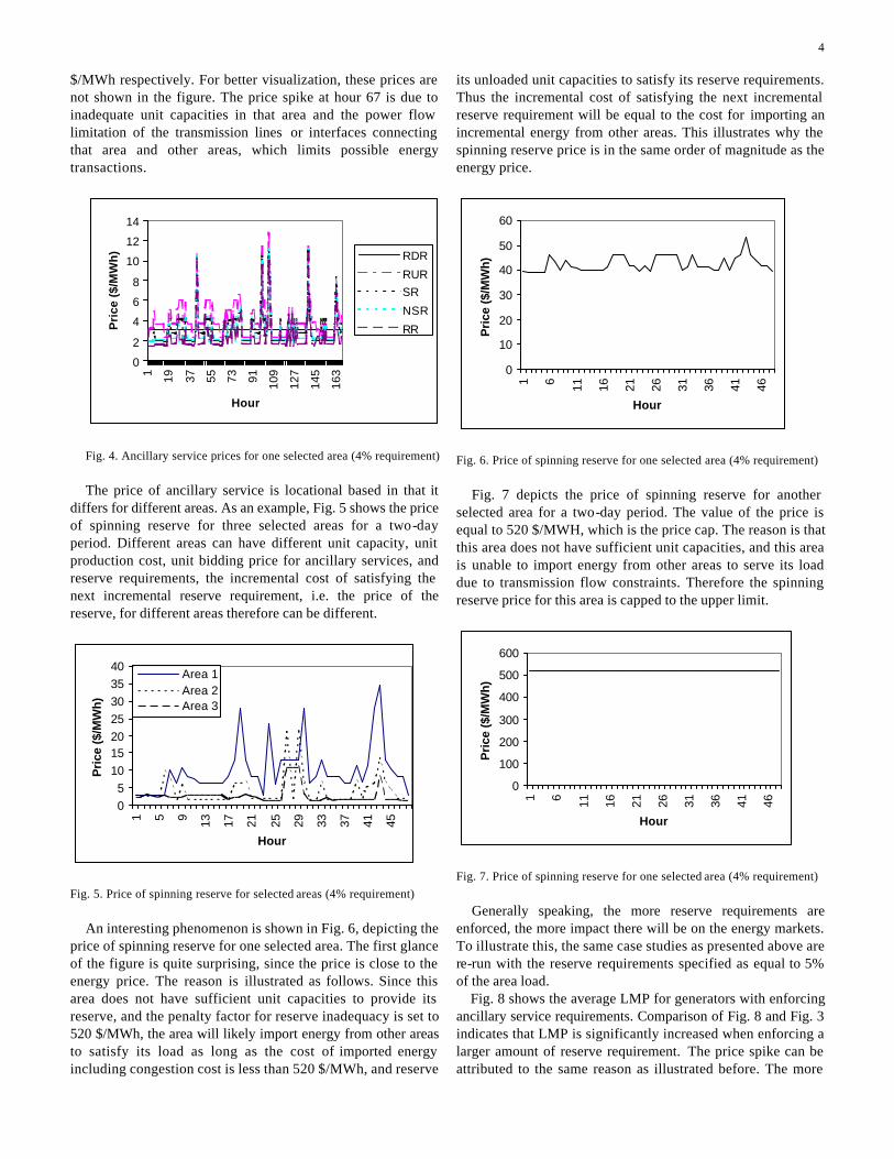
The prices of different types of ancillary services for one selected area are plotted in Fig. 4. The actual prices for RUR, SR, NSR and RR at hour 67 are 457.0, 456.7, 456.8, and 456.3
4
$/MWh respectively. For better visualization, these prices are not shown in the figure. The price spike at hour 67 is due to inadequate unit capacities in that area and the power flow limitation of the transmission lines or interfaces connecting that area and other areas, which limits possible energy transactions.
0
2
4
6
8
10
12
14
1 19 37 55 73 91 109
127
145
163
Hour
Pri
ce (
$/M
Wh
) RDR
RURSR
NSR
RR
Fig. 4. Ancillary service prices for one selected area (4% requirement)
The price of ancillary service is locational based in that it
differs for different areas. As an example, Fig. 5 shows the price of spinning reserve for three selected areas for a two-day period. Different areas can have different unit capacity, unit production cost, unit bidding price for ancillary services, and reserve requirements, the incremental cost of satisfying the next incremental reserve requirement, i.e. the price of the reserve, for different areas therefore can be different.
05
10152025303540
1 5 9 13 17 21 25 29 33 37 41 45
Hour
Pri
ce ($
/MW
h)
Area 1Area 2Area 3
Fig. 5. Price of spinning reserve for selected areas (4% requirement)
An interesting phenomenon is shown in Fig. 6, depicting the price of spinning reserve for one selected area. The first glance of the figure is quite surprising, since the price is close to the energy price. The reason is illustrated as follows. Since this area does not have sufficient unit capacities to provide its reserve, and the penalty factor for reserve inadequacy is set to 520 $/MWh, the area will likely import energy from other areas to satisfy its load as long as the cost of imported energy including congestion cost is less than 520 $/MWh, and reserve
its unloaded unit capacities to satisfy its reserve requirements. Thus the incremental cost of satisfying the next incremental reserve requirement will be equal to the cost for importing an incremental energy from other areas. This illustrates why the spinning reserve price is in the same order of magnitude as the energy price.
0
10
20
30
40
50
60
1 6 11 16 21 26 31 36 41 46
Hour
Pri
ce ($
/MW
h)
Fig. 6. Price of spinning reserve for one selected area (4% requirement)
Fig. 7 depicts the price of spinning reserve for another selected area for a two-day period. The value of the price is equal to 520 $/MWH, which is the price cap. The reason is that this area does not have sufficient unit capacities, and this area is unable to import energy from other areas to serve its load due to transmission flow constraints. Therefore the spinning reserve price for this area is capped to the upper limit.
0
100
200
300
400
500
600
1 6 11 16 21 26 31 36 41 46
Hour
Pri
ce ($
/MW
h)
Fig. 7. Price of spinning reserve for one selected area (4% requirement)
Generally speaking, the more reserve requirements are enforced, the more impact there will be on the energy markets. To illustrate this, the same case studies as presented above are re-run with the reserve requirements specified as equal to 5% of the area load. Fig. 8 shows the average LMP for generators with enforcing ancillary service requirements. Comparison of Fig. 8 and Fig. 3 indicates that LMP is significantly increased when enforcing a larger amount of reserve requirement. The price spike can be attributed to the same reason as illustrated before. The more

5
reserve required, the more likely it will be for that area to be unable to satisfy the reserve requirement, which can lead to the price spike.
0
100
200
300
400
500
6001 17 33 49 65 81 97 113
129
145
161
Hour
LM
P ($
/MW
h)
Fig. 8. Average LMP for generators with enforcing ancillary service requirements (5% requirement)
Price of the spinning reserve for selected areas are shown in Fig. 9. Comparison with results shown in Fig. 5 reveals that the price is significantly higher when the reserve requirement is increased. When the reserve requirement is increased, it is more likely for the reserve price to go up or approach the price cap since it is more likely that the reserve can not be satisfied due to insufficient generation resources and transmission flow limits.
0
100
200
300
400
500
600
1 6 11 16 21 26 31 36 41 46
Hour
Pri
ce ($
/MW
h)
Area 1Area 2Area 3
Fig. 9. Price of spinning reserve for selected areas (5% requirement)
The generation level and generation cost for selected areas is shown in Table II.
TABLE II GENERATION LEVEL AND COST FOR SELECTED AREAS (5%
REQUIREMENT)
Area 1 Area 2 Area 3 Area 4 Modeling
AS Generation (MWh) 307,859.0 926,362.0 269,414.0 9,369.0 No Generation (MWh) 303,109.0 933,284.0 296,627.0 59,859.0 Yes Generation Cost ($) 8,875,784.0 16,941,868.0 7,779,848.0 276,516.0 No Generation Cost ($) 10,025,788.0 17,282,256.0 8,849,072.0 2,503,235.0 Yes
Comparison with results shown in Table I indicates that different amount of reserve requirement can lead to different generation level and generation cost, since different amount of capacity will be set aside and different amount of energy importation will be transacted based on economic and system-security considerations. Not only can modeling one type of ancillary service markets impact the energy market, it can also bring about impact on another type of ancillary service market. Fig. 10-12 shows the price of RUR, NSR and RR when the spinning reserve is enforced or not enforced. Note that the results shown in the figures are based on simulation studies with reserve requirement set equal to 4% of area load. It is shown that generally the prices of RUR, NSR and RR are higher when enforcing the SR than those obtained when not enforcing the SR. Possible reasons are given as follows. When SR is enforced, the area has higher probability of needing energy importation, which may be more expensive and may also incur additional transmission congestion cost. In addition, some cheaper units may set aside part of its capacity for SR, and more expensive units may need to meet the energy demand. These factors could increase the price of other types of reserves.
0
2
4
6
8
10
12
1 5 9 13 17 21 25 29 33 37 41 45
Hour
Pri
ce (
$/M
Wh
)
Without SRWith SR
Fig. 10. Price of regulation up reserve with and without enforcing spinning reserve (4% requirement)

6
0
2
4
6
8
10
12
1 6 11 16 21 26 31 36 41 46
Hour
Pri
ce ($
/MW
h)
Without SR
With SR
Fig. 11. Price of non-spinning reserve with and without enforcing spinning reserve (4% requirement)
0
2
4
6
8
10
12
1 6 11 16 21 26 31 36 41 46
Hour
Pri
ce ($
/MW
h)
Without SR
With SR
Fig. 12. Price of replacement reserve with and without enforcing spinning reserve (4% requirement)
V. CONCLUSIONS
Ancillary service markets (regulation down, regulation up, spinning reserve, non-spinning reserve and replacement reserve) interact with the enery market and among themselves. To appreciate the nature and predict the consequences of these interactions, ancillary service markets are simultaneously cleared with the energy market in an integrated electricity market simulation program, GridView. Results from example system simulations demonstrate impact of ancillary service on the energy market, showing the significance and necessity of including ancillary service modeling in market analysis using a simulation software.
VI. DISCLAIMER
This paper does not necessarily reflect the viewpoints of ABB Inc. Any errors or omissions are the sole responsibility of the authors.
VII. REFERENCES [1] New England Power Pool, Market Rules & Procedures, February
27, 2002. [2] New York ISO, Ancillary Service Manual, July 15, 1999.
[3] New York ISO, System Operation Procedures, May 21, 2001. [4] New York ISO, Day Ahead Scheduling Manual, June 12, 2001. [5] PJM Manual for Scheduling Operations (M-11), December 1, 2002. [6] PJM Reserve Requirements (M-20), January 1, 2001. [7] 2003 ERCOT Methodologies for Determining Ancillary Service
Requirements, July 26, 2002 [8] X. Feng, L. Tang, Z. Wang, J. Yang, W. Wong, H. Chao, and R.
Mukerji, “An integrated electrical power system and market analysis tool for asset utilization assessment”, IEEE PES Summer Meeting, Chicago, July 2002.
[9] X. Feng, J. Pan, L. Tang, H. Chao, and J. Yang, “Economic evaluation of transmission congestion relief based on power market simulations”, IEEE PES General Meeting, 2002.U.S.
VIII. BIOGRAPHIES
Yuan Liao (M’2000) is with ABB Corporate Research USA. He currently works on projects related to developing algorithms and software for power market modeling and simulation, and large-scale resource scheduling optimization.
Xiaoming Feng (M’87) is an executive consulting R&D engineer with ABB Corporate Research in USA. He has over a dozen years of industry experience working as management consultant, R&D engineer, software developer and software product manager. His research interests include simulation, analysis, planning and optimization of electric power delivery and control systems using advanced simulation, optimization, probabilistic techniques, and information technology. In recent years, he was the principal investigator in research in high performance decomposition/relaxation techniques and general heuristics for large-scale resource scheduling, multi-step recursive techniques for short -term electricity price forecast, and simulation methodology for competitive electricity markets.
Jiuping Pan (M’97) received his B.S.E.E and M.S.E.E. from Shandong University of Technology, China, and then his Ph.D. in electrical engineering from Virginia Tech, USA. He is currently a principal consulting R&D engineer at ABB Corporate Research US. His main working experiences and research interests include generation and transmission planning, power system reliability assessment, network assessment management, and competitive market simulation studies.
Determination of Boiler Efficiency During Transient Conditions By Robert Kneile, Ph.D., Consulting Research Engineer, U.S. C.R.C. Abstract The determination of boiler efficiency is always based on the plant operating at steady-state conditions. In fact, the Power Test Codes go to great lengths to define what is considered steady-state for the purpose of boiler efficiency determination. Most modern data acquisition systems have algorithms for determining boiler efficiency based on real time data. In general, these boiler efficiency algorithms are based on the same steady-state computations, even though the plant may be going through transients. Hence, there is concern in the accuracy of computation of boiler efficiency during transient operation. This paper discusses the confidence that can be placed on the accuracy of boiler efficiency and proposes an alternative to refining the computations. Introduction According to the Power Test Codes, boiler efficiency is defined to be valid only when the data is collected as steady-state conditions. In analyzing the computations of boiler efficiency under transient conditions, referred to here as “dynamic boiler efficiency”, many components in the boiler are changing which affects the validity of the computations. Since by definition, boiler efficiency is only valid at steady-state conditions, the concept of dynamic boiler efficiency needs to be clarified. In this article, dynamic boiler efficiency is a quantity that would provide a realistic indicator of boiler efficiency as if it was calculated under steady-state conditions. How this quantity is determined is subjective since any set of measurements used for boiler efficiency calculation during transients will never represent steady-state operation. Discussion of dynamic boiler efficiency will focus upon the concept that energy is absorbed within the boiler when there is more energy going into the boiler than going out. The energy absorbed, in part, has potential to produce additional steam; hence, some of this energy should be credited in determining boiler efficiency. Likewise, when there is less energy going into the boiler than going out, there is a net depletion of energy within the boiler and boiler efficiency should be adjusted according.

Simple Definition of Boiler Efficiency The definition of boiler efficiency is kept simple to easily identify the main affects on the determination of boiler efficiency and to illustrate an approach for determining dynamic boiler efficiency. Results from the analysis can easily be applied to more complex boiler efficiency computations that may include numerous boiler credits and losses. Historically, boiler efficiency has been defined by both the input-output method and the heat loss method. Boiler efficiency by the input-output method is defined as:
%100FuelInHeat
FluidWorkingbyAbsorbedHeatoutputinput =−µ
For a boiler producing steam, the “Heat Absorbed by Working Fluid” is the sum of the individual steam supply line flow rates times their corresponding enthalpy rise.
∑ ∆= steamsteam HWFluidWorkingbyAbsorbedHeat The Heat In Fuel is defined as the fuel rate multiplied by the higher heating value of fuel.
fFHFuelInHeat = In terms of these quantities, the input-output method becomes:
%100f
steamsteamoutputinput FH
HW∑ ∆=−µ
Boiler efficiency by the heat loss method is defined as:
%1001 ⎟⎟⎠
⎞⎜⎜⎝
⎛−=
FuelInHeatLossesHeat
lossheatµ
or
%1001 ⎟⎟⎠
⎞⎜⎜⎝
⎛−=
f
Losslossheat FH
Qµ
Since the “Heat in the Fuel” is considered to be separated into “Heat Absorbed by Working Fluid” plus “Heat Losses”, the two efficiency equations are essentially equivalent at steady-state conditions. But this is only true under ideal conditions (measurements used for the two boiler efficiency calculations are not the same) and assumptions (e.g., heat loss due to surface radiation and convection applies to the heat loss method only and is usually approximated from a standard radiation loss chart).
2

Even if these two efficiencies are computed to be the same under steady-state conditions, they cannot be expected to be equal under dynamic conditions. One approach is to assume a dynamic boiler efficiency to be the average of the two efficiencies. This could be a poor approach for two reasons. First, there is no guarantee that a realistic dynamic boiler efficiency will even be between the two individual efficiencies. And second, one of the two boiler efficiencies might give a better value than the other under dynamic conditions. In the following discussion, these two issues become clarified. Definition of Dynamic Boiler Efficiency When a boiler is operating under transient conditions, many factors can contribute to the distortion of the efficiency calculation. The following is a partial list of items that can affect boiler efficiency calculations:
- thermal holdup in the boiler metal masses - thermal holdup in the boiler fluids - potential energy change with change in main steam pressure - dynamic lag of pulverizers - dynamic lag of sensors
Boiler dynamics is primarily affected by the large amount of holdup of both metal masses and fluid masses. Assuming this, the main contribution to dynamic boiler efficiency is primarily related to the thermal holdup. A dynamic energy balance on the boiler can be defined as:
Losssteamsteamf QHWFHdtdQ −∆−= ∑
where dQ/dt represents the change in thermal energy holdup resulting from dynamic conditions. While representing thermal holdup by a single quantity in a complex operation such as a boiler is an over-simplification, it nonetheless becomes useful in analyzing the boiler efficiency calculation under transient conditions. The dynamic boiler efficiency can now be defined as:
%100)/(
f
steamsteamdyn FH
dtdQKHW +∆= ∑µ
where K represents the fraction of dynamic thermal energy stored that will eventually be a contributing quantity to boiler efficiency.
3

Through algebraic manipulation, it is fortuitous that the dynamic heat rate can be defined in terms of a weighted average of the input-output and heat loss boiler efficiencies. ( )outputinputlossheatoutputinputdyn K −− −+= µµµµ When K is set to 1, the dynamic boiler efficiency becomes the boiler efficiency determined by the heat loss method; likewise, when K is set to 0, the dynamic boiler efficiency becomes the boiler efficiency determined by the input-output method. Hence, there is good reason to believe that a value representing dynamic boiler efficiency should be between the two individual efficiencies. Now, it would be beneficial to know if one of the two efficiency values provides a more realistic representation of the true operating efficiency. The following observations can be made from the above definition of dynamic boiler efficiency:
1. If the stored thermal energy will all be turned into useful steam (i.e., K =1), then boiler efficiency is better represented by the heat loss method.
2. If none of the stored thermal energy will be turned into useful steam (i.e., K =0), then
boiler efficiency is better represented by the input-output method. The difficulty lies in identifying the amount of stored energy that will be released with the steam and the remaining amount that will be lost. The issue is further complicated since the amount of heat absorbed in the boiler that is recoverable into steam is dependent upon what caused the transient and the rate at which the boiler goes back to steady-state conditions. Several mechanisms affecting the rate of energy holdup and the ability to recover this energy into useful steam production are identified here.
1. Most of the thermal energy stored in the steam/water due to increases in temperature or drum level is likely to be recovered as useful energy in the steam.
2. The energy stored in the pulverizer (i.e., extra coal) due to pulverizer transients
represents storage of extra coal. Hence, its thermal energy recovery should be no different than the current boiler efficiency.
3. Most of the thermal energy stored on the furnace side is expected to be lost with the
stack gas. However, the amount of thermal energy stored in furnace side of the boiler is considerably less than the energy stored elsewhere. This is evident by noting that the transients on furnace side are considerably faster that the steam/water side.
4. The thermal energy stored in the boiler tubes is the most difficult to reason where the
stored thermal energy end up. If the boiler transient was on the steam/water side, most of the stored thermal energy should return back to the steam/water, provided the transient was short enough to minimize the increase in the boiler surface temperature on
4

the gas side. For slower transients, the rise in tube surface temperature on the furnace side will start to reduce radiant heat transfer into the tube.
5. Heat loss by radiation is an important contributor to boiler efficiency, especially at low
load conditions. Yet, it is relatively constant with load changes. Hence, it should not play any significant role in boiler transients.
Based upon the above reasoning, much of the stored energy should go into the steam as transients are diminished. Thus, dynamic boiler efficiency is likely to be closer to realistic conditions when the value of K is near one. This implies that boiler efficiency by the heat loss method is probably a better indicator than the input-output method for boiler efficiency during transients. Boiler Dynamics Boiler dynamics can occur for many reasons. The following identifies several areas of plant dynamics, listed in the order of increasing severity.
- operating at a specific load condition (e.g., design load) with minimal load changes. - maneuvering from low load to design load (and vice versa) - plant equipment failure (e.g., mill trip or plant runback)
Intuitively, the more the plant is changing in operation, the less confidence there can be placed on boiler efficiency calculations. The severity of boiler dynamics can be defined in terms of rate of thermal energy absorbed, normalized to the amount of energy added to steam production.
∑ ∆
=steamsteam
S HWdtdQX /
Figure 1 identifies the relative effect of the different boiler efficiencies to the severity of boiler dynamics. When the boiler is going through mild dynamics, (identified by the first two cases above), XS should be below 0.05. At this condition boiler efficiency for K = 1 (heat loss method) and at K = 0.75 are relatively close to each other as one might expect. The true representation of the dynamic boiler efficiency should likely take on similar values. The boiler efficiency for K = 0 (input-output method) shows significant deviations, even when XS is at 0.05 and becomes much worse with increasing severity.
5

Figure 1 - Dynamic Boiler Efficiency
0.82
0.84
0.86
0.88
0.90
0.92
0.94
0.96
0.98
1.00
1.02
0.00 0.02 0.04 0.06 0.08 0.10 0.12 0.14 0.16 0.18 0.20Severity of Boiler Dynamics - (dQ/dt)/WdH
Nor
mal
ized
Boi
ler E
ffici
ency
u(d
yn) /
u(h
eat l
oss)
k=1.00 - u(heat loss)k=0.75k=0.50k=0.25k=0.00 - u(input-output)
Experimental Evaluation Ramping the boiler up in load is probably the most important transient period for computing boiler efficiency. If boiler efficiency is already known at a specific load condition (i.e., boiler efficiency determined at steady-state conditions), the value of K can be computed experimentally. Assuming the value of the dynamic boiler efficiency is representative of boiler efficiency at steady-state conditions, the above dynamic boiler efficiency equation can be solved for K:
⎟⎟⎠
⎞⎜⎜⎝
⎛
−
−=
−
−
outputinputlossheat
outputinputssKµµ
µµ
where
ssµ = boiler efficiency at steady state conditions
lossheatµ = boiler efficiency by heat loss method (computed under transient condition)
outputinput−µ = boiler efficiency by input-output method (computed under transient condition Using the above equation to solve for K at several load conditions, the value of K can now be determined as a function of load condition. Hence, an online determination of boiler
6
efficiency can be determined during load ramping that should better represent the true value of boiler efficiency. Conclusion A detailed analysis of boiler efficiency calculations under dynamic conditions, looking at all possible contributions to boiler dynamics, is not realistic. However, boiler dynamics represented as a container of thermal energy provides some insight into the performance of steady-state boiler efficiency calculations. Specific analysis of the various mechanisms of boiler dynamics indicates that boiler efficiency calculated by the heat loss method is not as susceptible error resulting from boiler transients as the input-output method. Hence, it would be the preferred value when considering just the two values. If both the heat loss and input-output boiler efficiencies are determined online, the better representation of boiler efficiency would be a weighted average of the two efficiencies. It is possible to determine the weighting factor experimentally. Once the weighting factor is known, future online boiler efficiency calculations based on the dynamic boiler efficiency algorithm should provide more realistic results. =================================================== Nomenclature F = Boiler fuel flow rate Hf = Higher heating value of fuel ∆Hstream = Enthalpy rise of steam in the boiler Qloss = Boiler losses
Q = heat absorbed by the boiler K = fraction of energy stored that will contribute to boiler efficiency
Wstream = Steam flow from the boiler XS = Severity of boiler efficiency µdyn = Dynamic boiler efficiency µheat loss = Boiler efficiency by the heat loss method µinput-output = Boiler efficiency by the input-output method µss = Steady-state boiler efficiency ============================================================ Note: Analysis of what happens in the boiler during transients is a very complex phenomenon, and is very subjective. Hence, other approaches for determining boiler efficiency during transients is possible, such as averaging the data over some specified length of time. In fact, averaging over a short time period should do well to smooth out the fast dynamics on the furnace side.
7

Biography Robert Kneile is a Consulting Applications Engineer at the ABB’s Corporate Research Center in Wickliffe, Ohio. At ABB, Dr. Kneile has been involved in model predictive control, dynamic reconciliation of data and asset monitoring. His previous experience at Bailey Controls include development of online power plant performance calculations and operating training simulators. A member of AIChE, he holds B.S. and M.S. degrees in Chemical Engineering from the University of Missouri at Columbia and Ph.D. degree in Chemical Engineering from Purdue University.
8
1. INTRODUCTION
The contoured parts that are commonly finished using
multiple axes milling machines, profilers, or by hand-held methods can also be finished using a robot along with belt grinding equipment. Owing to the higher flexibility of the robotic belt grinding workcell, this configuration offers greater versatility when dealing with many fabricated parts having irregular contoured shapes. Compared with conventional grinding processes, robotic belt grinding is more forgiving, cost effective, and introduces more versatility into many grinding and finishing operations. Depending on the application, the robotic belt grinding can be used either to achieve relatively high material removal rates and/or satisfactory surface finishes.
At present, robots are commonly employed in many conventional metal-grinding applications. However, unlike the conventional grinding process in which the grinding wheels used are relatively rigid, the abrasive element in robotic belt grinding is far more flexible. Therefore the conventional grinding process modeling cannot directly be applied. Since the use of flexible belt grinding equipment in manufacturing applications is relatively recent, currently there is a negligible amount of published information available in this field. Thus, the primary objective of this study is to develop a process model suitable for the application of flexible belt grinding equipment as utilized in robotic material grinding applications.
2. NOMENCLATURE
a Depth of cut, mm Ac Contact area between the grinding wheel and
workpiece, mm2/mm Fth Threshold force to removal the material from
workpiece, N/mm2 WRP Material removal parameter, mm3/s, N MRR Material removal rate, mm3/s, mm Fn Normal force, N/mm R Contact wheel radius, mm L Contact length, mm θ Contact angle, degree ∆ Contact wheel deformation, mm V Workpiece infeed rate, mm/s Cr Robot compliance, mm/N Cw Grinding compliance, mm/N Ct Equivalent tooling compliance, mm/N
Cg Grinding loop compliance, mm/N
rX∆ Robot deformation, mm
tX∆ Tool wear, mm
gX∆ Grinder displacement, mm
ε Deformation coefficient
3. OVERVIEW OF GRINDING PROCESS MODELING
Many researchers and engineers have made a great effort to develop the process modeling for grinding process. Hahn [1] described the conventional grinding process by the “Wheelwork Characteristic Chart” using the relationship between the volumetric rates of stock removal and the normal interface force intensity. It was shown that the sharpness of the grinding wheel will be decreased as wear flat develops on the abrasive grains.
When robotic grinding was emerged, researchers have tried to apply conventional grinding process model to flexible robotic grinding. Most previous work has been done in robotic deburring or disk grinding [2]. A static model [3] and dynamic model [4] for robotic disk grinding system were established by Whitney and Brown. In those conventional models, workpiece cutting stiffness and grinding wheel wear stiffness are simply defined as a constant dxFKw = and
dsFK s = . Persoons and Vanherck [5] built a model based on experimental results for robotic cup wheel grinding. Persoons’s model confirmed the well-known behavior in conventional grinding that the workpiece material removal rate is proportional to the exerted force.
All of the previous models are based on the assumption that the contact area between the workpiece and grinding wheel is simple-point-contact. As a result, the contact area is treated as constant and process modeling is a simplified relationship between the normal force and the material removal rate.
In robotic belt grinding, the contact area between the abrasive surface and workpiece varies, and as a consequence, the grinding force always varies in the grinding process even though the depth of cut is a constant. Literature searches have not identified any information regarding the compliant nature of the belt grinding process. The preliminary test results conducted in this research have identified significant differences between robotic belt grinding and conventional grinding.
Process Modeling of Flexible Robotic Grinding
Jianjun Wang*, Yunquan Sun*, zhongxue Gan*, and Kazem Kazerounian **
* Robotic & Automation, ABB Corporate Research, USA (Tel : +1-860-285-6964; E-mail: [email protected])
**Department of Mechanical Engineering, University of Connecticut, CT, USA (Tel : +1-860-486-2251; E-mail: [email protected])
Abstract: In this paper, an extended process model is proposed for the application of flexible belt grinding equipment as utilized in robotic grinding. The analytical and experimental results corresponding to grinding force, material removal rate (MRR) and contact area in the robotic grinding shows the difference between the conventional grinding and the flexible robotic grinding. The process model representing the relationship between the material removal and the normal force acting at the contact area has been applied to robotic programming and control. The application of the developed model in blade grinding demonstrates the effectiveness of proposed process model. Keywords: process modeling, robotic grinding, blade, material removal rate

ICCAS2003 October 22-25, Gyeongju TEMF Hotel, Gyeongju, Korea
Therefore, it is necessary for robotic industry to develop the process modeling to adapt into flexible robotic grinding. Based on the study of the material removal mechanism and the dynamic characteristics of the associated robot, process characterization will be investigated in an attempt to obtain appropriate process input-output relationships. This part of the study will establish the basic process modeling for a flexible belt grinding process from both analytical and experimental results.
4. THEORETICAL ANALYSIS OF ROBOTIC
GRINDING PROCESS MODEL 4.1 Basic process model in robotic grinding
In order to effectively investigate the new process model, the basic concepts set forth by Hahn and Lindsay will be pursued in this study. However, further considerations that must be addressed are summarized as: 1) In conventional grinding, flat or cylindrical, the applied
equivalent diameters are in most times considered to be constant. However, a belt grinding process is more commonly applied to parts having irregular contours and local curvature must be considered. The real area of contact is far more complicated than in conventional grinding. It is not only related to the development of wear flats on the abrasive grains, but also related to the other important parameters such as the local curvature of the workpiece, contact wheel hardness and diameter, belt tension, belt properties.
2) The surface speed of the grinding wheel is an important parameter in the conventional grinding process. Because of the variation of belt grinding contact area during the grinding process, the workpiece infeed rate must be controlled in an effort to maintain a more or less constant rate of material removal.
3) Because of the relative flexibility of belt grinding elements, it is anticipated that the threshold force behavior is considerably different from that of conventional grinding.
Considering those factors, this study will focus on the relationship among the normal cutting force, the MRR and the contact area, which can be described by the following equation:
nthc FWRPMRRFA =+⋅ / (1) Where:
Ac Contact area between the grinding wheel and workpiece, mm2/mm;
Fth Threshold force to removal the material from workpiece, N/mm2;
WRP Material removal parameter ( Nsmm ,3 ), which is the material removal rate under unit force;
MRR Material removal rate ( mmsmm ,3 ); Fn Normal force, N/mm.
Rewriting Eq. (1) as: [ ] cnthc AFFAWRPMRR =+× (2) This rewriting indicates the following facts: 1) While the contact area changes significantly during the
grinding process, contact area becomes a variable in process model. Therefore, the process model is a 3D relationship among force, MRR and contact area.
2) When the contact area is considered, the robotic grinding process is not constant force control, but constant pressure control.
3) Considering force, MRR and contact area as three variables, Fth and WRP determined by abrasive tool will be treated as the model parameters to be determined.
FN
MRRAC
Fth plane(blunt belt)
Fth
Fth plane(fresh belt)
Fig. 1 Relationship among MRR, Contact Force, FN and
Contact Area, AC under Different Belt Conditions
Fig. 1 shows the comparative relationships of FN, MRR, and AC, based on Eq. (1) for fresh and blunt grinding belts. Consistent with the result from Hahn, it can be seen that a force can be supported between a grinding wheel and workpiece without material removal taking place. This region is known as the “rubbing zone”. When the force exceeds a critical value, material removal takes place, initially non-linearly known as the “plowing zone”. As the force is increased further the removal rate increases linearly in the region known as the “cutting zone”. A two dimensional model by taking a section parallel to the plan consisting of FN and MRR axes show in Fig. 1 will be identical to the model developed by Hahn [1]. In addition, this 3D model considers the nature of the robotic grinding with flexible contact wheel and different curvature of the workpiece.
Contact wheel
Material to be removed
Contact area
Geometric error
Fig. 2 Effect of workpiece geometric error on contact area, AC
Considering
VaMRR ×= (3) Where a Depth of cut, mm V Workpiece infeed rate, mm/s Thus, Eq. (2) can be further rewritten as:
( ) ( ) thcnc FAFWRPAVa −=×× (4) This equation further reveals the relation among actual
depth of cut with feed speed and contact area. Fig. 2 shows the change in AC resulting from a geometric error on the workpiece for a hypothetically stiff roller. In practice, the roller will usually be flexible and there will be flattening of the contact wheel. Based on the hardness of the contact wheel and the kind of the grinding belt backing, a theoretical model will be developed in this study. Preliminary tests made by

ICCAS2003 October 22-25, Gyeongju TEMF Hotel, Gyeongju, Korea
measuring the difference between the displacement of the contact wheel and the real motion of the robot have shown that the contact area varies with the change of contact wheel hardness, belt tension, and workpiece geometry. 4.2 Local curvature in flexible robotic grinding vs equivalent Diameter in conventional grinding
From Eq. (4), it is observed that the local curvature will significantly affect the grinding force. In order to consider the effect of the cutting action for the difference in curvature of the wheel and work in the contact region in the conventional grinding process, Hahn [1] related the difference of curvature of internal or external grinding to the surface grinding by considering an equivalent diameter. Due to the characteristic of the robotic grinding process, such as the flexible contact wheel, the flexible robot arm, and the complex geometry of the workpiece, the equivalent diameter cannot be used in this process. Instead the local curvature is introduced to consider the change of the contact area during the grinding process. A speed factor will be calculated based on the normalized local curvature. The robot speed is adjusted according to the speed factor for each process point. The maximum speed of the path will be determined by the process model, which will be discussed in detail in the next section. 4.3 Contact stiffness and deformation
Process modeling describes the relationship of grinding force and depth of cut. However, actual depth of cut is affected by the overall system deformation. Therefore overall system model needs to be considered while applying the process modeling into robotic process control. Fig. 3 illustrates the compliant nature of the overall flexible robotic grinding system. A description of the appropriate terms is given as:
(9)
Contact wheel
Force sensor
Nominal path Robot arm
Grinding belt
Real path
rC
wC
tC
gC
Fig. 3 Compliances in Robotic Belt Grinding
( )
( )n
rr FforceNormal
xndeformatioRobotCcomplianceRobot
∆=
(5) ( )( )n
w FforceNormalacutofDepth
CcomplianceGrinding = (6)
( )n
tt FforceNormal
XToolwearCcompliancetoolingEquivalent
)(∆= (7)
( )n
gg FforceNormal
XGrinderCComplianceLoopGrinder
)(∆= (8)
The total compliance between the workpiece and the
grinding surface is formulated as:
gtwr
n
g
n
t
nn
r
n
totaltotal
CCCC
F
X
FX
Fa
FX
FX
C
+++=
∆+
∆++
∆=
∆=
(9)
It is obvious that when the normal force exists between the workpiece and the grinding tool, the deformations of the robot, the grinding wheel and the workpiece have to be considered if an accurate depth cut is obtained. The true depth of cut will be the total commanded displacement with subtraction of wheel deformation, robot arm deformation and wheel movement. Based on this fact, the process model in Eq. (4) will be rewritten as:
( )[ ]th
c
n
c
ngtrTotal FAF
WRPA
VFCCCX−=
×××−−−∆
(10)
( ) thc
n
c
Total FAF
VWRPA
VX−⋅+=
⋅⋅∆ ε1 (11)
where:
( )
WRP
CCC gwr ++=ε (12)
and ∆XTotal is the robot commanded displacement, V is robot speed. This expression provides a robot control format for a flexible grinding process.
As shown in Fig. 4, a special experiment was performed to investigate deformation effects on the contact area. In this test, the robot arm holds the workpiece and pushes against the contact wheel. LVDT 1 and LVDT2 are used to measure the grinding wheel motion and the robot arm motion respectively. An ATI force/torque sensor is used to monitor the contact force. The belt tension pressure is 2 bars and the air cylinder pressure to support the contact wheel is 3.0 bars.
Force sensor
Robot Arm
GripperWorkpieceGrinding belt
Contact Wheel
LVDT 1
LVDT 2
Contact length
Fig. 4 Contact Area and Contact Stiffness Testing
Fig. 5 shows a clear picture of the robot compliance, wheel compliance and the grinding wheel and robot movement. It can be observed that the total command displacement has been divided into four portions: robot deformation, robot movement, grinding wheel deformation and grinding wheel movement.
As the robot approaches the grinding wheel, the force between the robot and the wheel will build up. Before the system reaches its critical stiffness, the robot and the grind wheel will be deformed due to the built-up force. The actual movement of the robot and the grinding wheel is smaller than the command displacement. When the system reaches the critical stiffness, the contact force is balanced with the air cylinder support pressure. At and after this critical point, the
ICCAS2003 October 22-25, Gyeongju TEMF Hotel, Gyeongju, Korea
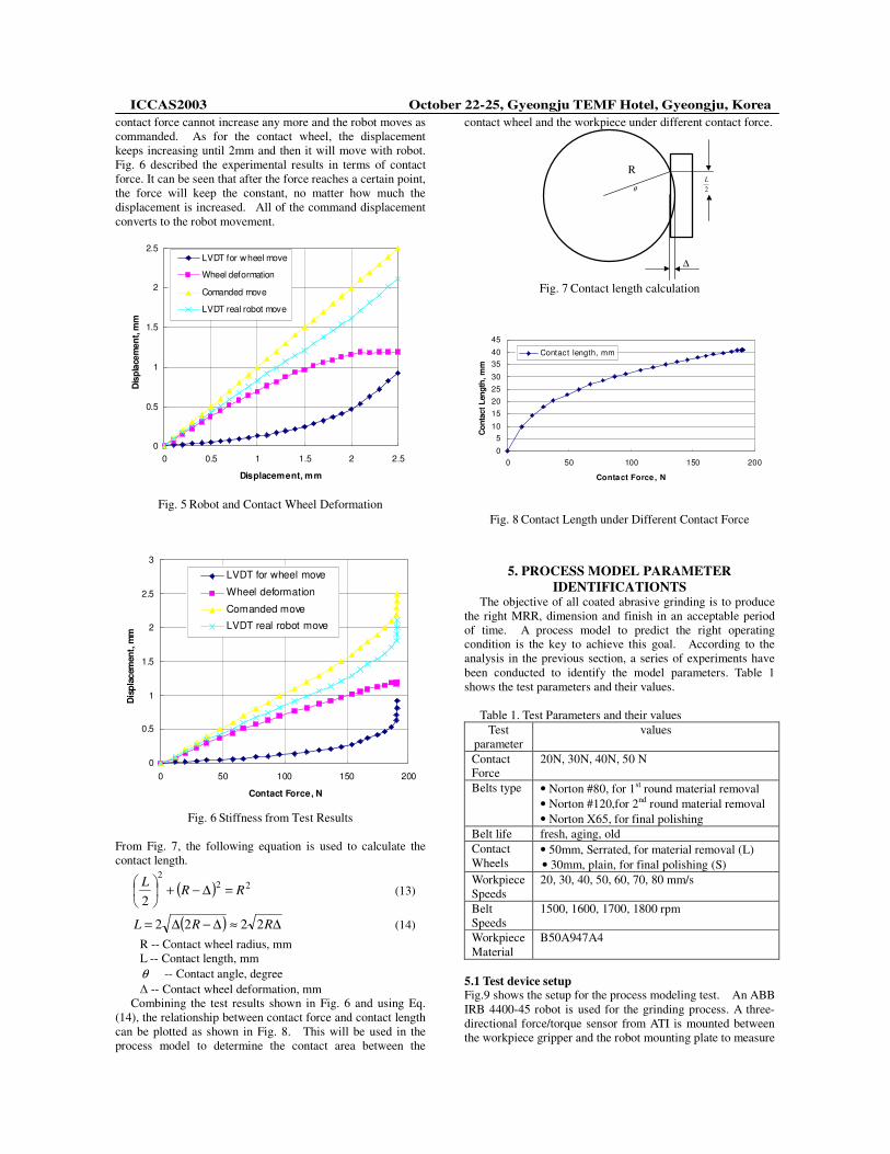
contact force cannot increase any more and the robot moves as commanded. As for the contact wheel, the displacement keeps increasing until 2mm and then it will move with robot. Fig. 6 described the experimental results in terms of contact force. It can be seen that after the force reaches a certain point, the force will keep the constant, no matter how much the displacement is increased. All of the command displacement converts to the robot movement.
0
0.5
1
1.5
2
2.5
0 0.5 1 1.5 2 2.5
Displacement, mm
Dis
plac
emen
t, m
m
LVDT for wheel move
Wheel deformation
Comanded move
LVDT real robot move
Fig. 5 Robot and Contact Wheel Deformation
0
0.5
1
1.5
2
2.5
3
0 50 100 150 200
Contact Force, N
Dis
plac
emen
t, m
m
LVDT for wheel move
Wheel deformation
Comanded move
LVDT real robot move
Fig. 6 Stiffness from Test Results
From Fig. 7, the following equation is used to calculate the contact length.
( ) 222
2RR
L =∆−+��
���
� (13)
( ) ∆≈∆−∆= RRL 2222 (14) R -- Contact wheel radius, mm L -- Contact length, mm θ -- Contact angle, degree � -- Contact wheel deformation, mm
Combining the test results shown in Fig. 6 and using Eq. (14), the relationship between contact force and contact length can be plotted as shown in Fig. 8. This will be used in the process model to determine the contact area between the
contact wheel and the workpiece under different contact force.
R
2L
θ
∆
Fig. 7 Contact length calculation
0
510
15202530
3540
45
0 50 100 150 200
Contact Force , NC
onta
ct L
engt
h, m
m
Contact length, mm
Fig. 8 Contact Length under Different Contact Force
5. PROCESS MODEL PARAMETER IDENTIFICATIONTS
The objective of all coated abrasive grinding is to produce the right MRR, dimension and finish in an acceptable period of time. A process model to predict the right operating condition is the key to achieve this goal. According to the analysis in the previous section, a series of experiments have been conducted to identify the model parameters. Table 1 shows the test parameters and their values.
Table 1. Test Parameters and their values
Test parameter
values
Contact Force
20N, 30N, 40N, 50 N
Belts type • Norton #80, for 1st round material removal • Norton #120,for 2nd round material removal • Norton X65, for final polishing
Belt life fresh, aging, old Contact Wheels
• 50mm, Serrated, for material removal (L) • 30mm, plain, for final polishing (S)
Workpiece Speeds
20, 30, 40, 50, 60, 70, 80 mm/s
Belt Speeds
1500, 1600, 1700, 1800 rpm
Workpiece Material
B50A947A4
5.1 Test device setup Fig.9 shows the setup for the process modeling test. An ABB IRB 4400-45 robot is used for the grinding process. A three- directional force/torque sensor from ATI is mounted between the workpiece gripper and the robot mounting plate to measure

ICCAS2003 October 22-25, Gyeongju TEMF Hotel, Gyeongju, Korea
Contact wheel
Force sensorRobot Arm
Gripper Workpiece
Grinding belt
Motor
Z
FyFT
Fz
Robotmovingdirection
YContact wheelrotate direction
Fig. 9 Process Modeling Testing Setup
the contact force between the workpiece and the grinding belt.
5.2 Process model testing results In this section, the test results for the Material Removal Rate under different operating conditions are illustrated. The test results include the MRR under different:
• Contact forces between workpiece and contact wheel • Belt life • Belts type and grit size • Belt speeds • Contact wheels (Large and small, plain and serrated)
Fig. 10 shows the material removal under different contact force and robot speed (Feedrate).
0
0.01
0.02
0.03
0.04
0.05
0.06
0.07
20 30 40 50 60 70 80
Robot Speed, mm/s
Mat
eria
l Rem
oval
, mm
20 N30 N40 N
50 N
• Contact wheel diameter: 400 mm• Contact wheel hardness: 30• Contact wheel type: Plain• Belt speed, 1500 rpm• Workpiece Material: B50A947A4• Contact force setup: 20 to 50 N• Belt: Norton SG R495 P80
Fig. 10 Material removal under different contact force and
robot speed
According to Eq. (3) and Eq. (4), if the grinding pressure keeps constant, then the relationship between the material removal (depth of cut) and the robot speed (feed rate) can be obtained as:
( ) WRPAFFVa cthn ⋅⋅−=⋅ (15)
If ( ) WRPAFF cthn ⋅⋅− keeps constant, thus
.ConstVa =× (16) which is a hyperbola curve. With difference force set-up values, the hyperbola curve will change its position in the
graphics. The experimental results shown in Fig. 10 prove the feasibility of model.
During this test, the lowest robot speed observed is higher than 20mm/s. Below this speed, the workpiece burn happened. On the other hand, the robot speed has to be limited under 50 mm/s to keep the reasonable material removal in production.
0
0.01
0.02
0.03
0.04
0.05
0.06
0.07
0 10 20 30 40 50 60 70
Force, NM
ater
ial R
emov
al, m
m
20 mm/s30 mm/s40 mm/s
50 mm/s60 mm/s70 mm/s
80 mm/s
Fig.11. Threshold Force Under Different Robot Speed
From Eq. (2), the relationship between the material removal and the contact force is described by a linear equation, as shown in Fig 11. The threshold force thF is the offset of this line equation, while WRP is the slope.
thC
n FAF
WRPMRR −= (17)
���
����
�−= th
c
n FAF
WRPMRR (18)
Due to the additional flexibility of the belt grinding elements, it is anticipated that the threshold force behaviors considerably different from that of conventional grinding. This is because the extra flexibility will make the belt relatively sharper, which in turn increases WRP and further causes the reduction of the threshold force.
In grinding process, belt wear is another reason to cause the inconsistent workpiece finish. The common methods to compensate the belt wear include:
• Increase the contact force; • Increase the belt speed; Since increasing contact force will create more chance for
the workpiece burn, the method of increasing belt speed is widely used. Fig. 12 shows that increasing the belt speed can increase the material removal effectively.
Belt types and grit size also affect WRP. To compare the performance of different belt types and grit sizes, both fresh belt (shown in Fig. 13) and the aging belt are tested. The Norton P80 and P120 are used to compare the same type of belts with different grit size. As can be seen, the material removal for fresh P80 and P120 belts does not make much difference. But the workpiece temperature will be much lower if using P80 rather than P120.
Fig 14 demonstrates the influence of the wheel size on the material removal rate. Under the same process condition, the smaller serrated contact wheel will produce a much larger
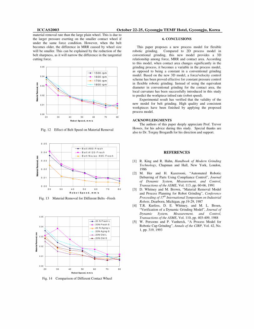
ICCAS2003 October 22-25, Gyeongju TEMF Hotel, Gyeongju, Korea
material removal rate than the large plain wheel. This is due to the larger pressure exerting on the smaller contact wheel if under the same force condition. However, when the belt becomes older, the difference in MRR caused by wheel size will be smaller. This can be explained by the reduction of the belt sharpness, as it will narrow the difference in the tangential cutting force.
0.00
0.01
0.02
0.03
0.04
0.05
2 0 30 40 50 60 70 80
Rob o t Sp e e d, m m /s
Mat
eria
l Rem
oval
, mm
15 00 rpm16 00 rpm
17 00 rpm18 00 rpm
Fig. 12 Effect of Belt Speed on Material Removal
0 .0 0
0 .0 1
0 .0 2
0 .0 3
0 .0 4
0 .0 5
2 0 3 0 4 0 5 0 6 0 7 0 8 0
R o b o t S p e e d , m m / s
Mat
eria
l Rem
oval
, mm
B e l t # 8 0 - F r e s h
B e l t # 1 2 0 - F r e s h
B e l t N o z a c X 6 5 - F r e s h
Fig. 13 Material Removal for Different Belts –Fresh
0 .00
0 .01
0 .02
0 .03
0 .04
0 .05
20 30 40 50 60 70 80
Robot Spe e d, m m /s
Mat
eria
l Rem
oval
, mm
20 N-F resh-L
20 N-F resh-S
20 N-A g ing-L
20 N-A g ing-S
20 N-Old-L
20 N-Old-S
Fig. 14 Comparison of Different Contact Wheel
6. CONCLUSIONS
This paper proposes a new process model for flexible
robotic grinding. Compared to 2D process model in conventional grinding, this new model provides a 3D relationship among force, MRR and contact area. According to this model, when contact area changes significantly in the grinding process, it becomes a variable in the process model, as opposed to being a constant in a conventional grinding model. Based on the new 3D model, a force/velocity control scheme has been proved effective for constant pressure control in flexible robotic grinding. Instead of using the equivalent diameter in conventional grinding for the contact area, the local curvature has been successfully introduced in this study to predict the workpiece infeed rate (robot speed).
Experimental result has verified that the validity of the new model for belt grinding. High quality and consistent workpieces have been finished by applying the proposed process model.
ACKNOWLEDGMENTS
The authors of this paper deeply appreciate Prof. Trevor Howes, for his advice during this study. Special thanks are also to Dr. Torgny Brogardh for his direction and support.
REFERENCES
[1] R. King and R. Hahn, Handbook of Modern Grinding Technology, Chapman and Hall, New York, London, 1986
[2] M. Her and H. Kazerooni, “Automated Robotic Deburring of Parts Using Compliance Control”, Journal of Dynamic System, Measurement, and Control, Transactions of the ASME, Vol. 113, pp. 60-66, 1991
[3] D. Whitney and M. Brown, “Material Removal Model and Process Planning for Robot Grinding”, Conference Proceeding of 17th International Symposium on Industrial Robots, Dearborn, Michigan, pp.19-29, 1987
[4] T.R. Kurfess, D. E. Whitney, and M. L. Broen, “Verification of a Dynamic Grinding Model”, Journal of Dynamic System, Measurement, and Control, Transactions of the ASME, Vol. 110, pp. 403-409, 1988
[5] W. Persoons and P. Vanherck, “A Process Model for Robotic Cup Grinding”, Annals of the CIRP, Vol. 42, No. 1, pp. 319, 1993

EXPERIENCES IN APPLYING AGILE SOFTWARE DEVELOPMENT PRACTICES IN NEW PRODUCT DEVELOPMENT
Aldo Dagnino1, Karen Smiley1, Hema Srikanth2, Annie I. Antón2, Laurie Williams2
1 ABB US Corporate Research, {aldo.dagnino, karen.smiley}@us.abb.com 1021 Main Campus Drive, Raleigh, NC, 27606, USA
2 North Carolina State University, {hlsrikan, aianton, lawilli3}@ncsu.edu 900 Main Campus Drive, Raleigh, NC, 27695, USA
ABSTRACT Experiences with software technology development projects at ABB Inc. indicated a need for additional flexibility and speed during explorations of applying new technologies to future products. A case study was conducted at ABB to compare and contrast the use of an evolutionary-agile approach with a more traditional incremental approach in two different technology development projects. The study indicated benefits associated with the evolutionary approach with agile practices, such as streamlined documentation, increased customer involvement, enhanced customer satisfaction, increased capability to include emergent requirements, and increased risk management ability. This paper suggests that using agile practices during the Research and Development (R&D) phase of new product development contributes to improving productivity, to increasing value-added activities, to showing progress early in the development project, and to enhancing customer satisfaction. Another observation derived from this study is that by offering a carefully selected subset of agile practices, ABB R&D groups are more likely to successfully incorporate them into their existing processes. KEY WORDS New software-intensive product development, agile practices 1. Introduction ABB Inc.1 is a multi-national corporation that develops products, largely software-intensive, for the power and automation technology market segments. Before a decision is made to begin a new project, a feasibility study is carried out to ensure that a resulting product is likely to have good economic potential [1]. After a working prototype is developed at the Corporate Research Center (CRC) lab, this prototype is turned into a product, or “productized,” by the Business Unit (BU). To ensure maximum efficiency, suitable lifecycles and processes need to be applied during the various development phases.
The ABB Software Process Initiative (ASPI) group, an international team of in-house product development process engineers, acts as the internal ABB Corporate Engineering Process Group (CEPG) and helps BUs choose the most efficient product development processes to optimize time, quality, and functionality [2, 3, 4, 5, 6, 7]. The ASPI group has deployed research and development techniques to improve speed and flexibility in software-intensive product development. Early in the year 2001, a two-stage Incremental Development Model (IDM) was created, tailored, and deployed by the ASPI group. After several technology development projects were carried out using this model, a need for further flexibility and speed sparked the creation of a more flexible and more agile Evolutionary Development Model (EDM) [5]. This paper reports on a case study that compares the incremental and the evolutionary models applied to two technology development projects at ABB. The projects were of similar size and comparable complexity. The estimated development time was under one calendar year for each project. The same team of five people developed both prototype-working systems (which served as the basis for the final products) in parallel. Our research goal for this study was to identify the process model more suitable for technology development projects and ABB. Using the Goal-Question-Metric approach [8], we defined the research question and metrics that needed to be collected to answer the research question. Question: Which process model is more effective for technology development projects: incremental or evolutionary? To answer this question, we determined that five metrics should be collected:
a. Time spent on documentation and project planning b. Customer involvement and satisfaction c. Requirements volatility d. Delivery of business value e. Risk reduction

Details on how these measures were defined and gathered are provided below. 2. Application of Agile Practices in ABB Research & Development In this section, we discuss ABB’s product development cycle. We also provide information on the software processes that were developed and used for technology development projects. 2.1. The ABB Product Development Cycle The product development cycle at ABB includes three primary phases, as shown in Figure 1. During the Feasibility Study Phase, a product idea is evaluated based on its potential business value and technological feasibility. The Technology Development (TD) Phase is associated with the activities performed to evaluate in greater depth the technological feasibility and business value of the proposed product. These initial development activities are primarily executed by the ABB CRCs, with involvement from the ABB BUs. TD projects at ABB typically last 6-12 months. The primary deliverable from the TD phase is a working prototype system that has the primary functionality of the intended final product. The third phase is the Product Development (PD) Phase, during which the prototype system is further enhanced and developed into a product by the BU that is responsible for sales to external customers and for supporting and maintaining the final product. ABB uses a “Gate Model” (GM) [1] to evaluate the business value of potential new products, to help ensure consistent execution and sound decision-making throughout the development lifecycle. Formal business decision processes like the ABB GM generally consist of different development stages, separated by business-decision evaluation points known as gates. Figure 1 shows the gates (numbered 0 through 7) of the ABB Gate
Model, and how the TD and PD phases are synchronized. Using the ABB Gate Model, achievement of predetermined pre-gate milestones is evaluated and business decisions are made on whether the project should be continued, amended, or stopped. 2.2. ABB Incremental Product Development In early 2001, an evaluation of the software development models used at ABB revealed that the traditional "waterfall" or Big Design Up Front (BDUF) [2] model was most commonly used within ABB development groups. However, the BDUF models did not always suit the needs of rapid-development TD projects within ABB. The exploratory nature of the projects and associated volatility of the requirements exacerbates the high documentation burden of BDUF models, frustrating the development teams and increasing the costs of adapting to shifts in technological direction based upon early discoveries from the feasibility assessments. For those projects in which the requirements are not highly volatile and the scope of the project can be defined early in the project, using an IDM is appropriate. Traditionally, an IDM had been used in TD activities at ABB. This incremental process incorporated small releases (in two increments of 2-4 months each) and a sound software development discipline. Given the desired time-to-market, the period from Gates 2-5 was expected to span a short period of time, so using more than two increments was viewed as impractical. However, an assessment of the amount of effort invested in documenting the requirements, managing the project, and preparing for (sometimes repeated) gate meetings for projects in the TD phase revealed that a “leaner” development model might be beneficial. Additional analyses showed that there was also significant room for improvement in speed, flexibility to accommodate emerging requirements, customer focus, customer engagement, and developer-friendliness. As a result of this evaluation, two initiatives were undertaken: Continued process streamlining and reduction of the
artifacts associated with the incremental model; and Creation of an agile process alternative.
Figure 1. ABB Product Development Phases and Gates
Technology Development Phase
Product Development Phase
G0 G1 G2 G3 G4 G5 G6 G7Corporate Research
Organization
Business Unit
Product
Feasibility Study Phase
FeasibilityStudy Report
PilotRelease
G0 G1 G2 G3 G4 G5 G6 G7

The second initiative will be discussed in the following two subsections. 2.3. Agile Product Development: ADEPT Agile Development in Evolutionary Prototyping Technique (ADEPT) [5, 10] was developed to increase agility and maturity on TD projects. Although several existing agile processes and lifecycle models [2, 3, 6] were considered, we decided to use a traditional evolutionary lifecycle model as a base model and add a subset of agile practices to that model to create ADEPT [5, 9]. It has been our experience that ABB development groups who are accustomed to more traditional software development approaches are able to accept more easily a gradual approach to incorporating agile practices, as provided by ADEPT, versus attempting to transition immediately to a fully agile methodology. Figure 2 provides a graphical representation of ADEPT. The ovals portray process activities, curved rectangles represent the artifacts, thicker arrows indicate control flows through the process, and the narrower arrows indicate data flowing as a result of the activities. The ADEPT model has three primary stages: During the Project Evaluation stage, team members
meet with the customer to negotiate project scope, gather system features, assign feature responsibility to team members or groups within the project team, and negotiate features to be implemented in the upcoming iteration. The Feature Development stage encapsulates the
activities performed in an ADEPT iteration. During this stage, developers may employ “agile” practices to plan, design, develop, test, and integrate features. At the beginning of the stage, the group meets with the customer to identify and negotiate the requirements to be implemented in the iteration. After the negotiation process, each team member or group concurrently plans, implements, and tests the requirements for the assigned features. During the initial customer evaluation, the customer suggests additions or revisions. These suggestions are addressed by applying additional feature development stages or iterations as needed. During the Project Completion stage, the
development team validates the system, delivers the system (pilot or prototype) to the customer, and conducts a project evaluation. The working prototype is given to the BU responsible for productizing it.
By having an evolutionary lifecycle model, an important agility principle was included in ADEPT: the ability to incrementally enhance the functionality of the software and thus allow for flexible adaptation to changing requirements.
Project Evaluation Stage
Feature Development Stage( Evolutions )
Risk-MitigationMeetings
FunctionalTesting
Gather Features Assign Feature Responsibility to Team's Groups
Feature Implementation
Feature Testing and Integration Initial Customer
Evaluation
Negotiate Project Scope
WhiteboardDesign
Feature Planning and Design
Final Customer Validation and
Product Delivery
Negotiate Feature Requirements
Project Completion Stage
Project Evaluation
Negotiate Evolution's Features
Project Plan -Requirements
Worksheet
AcceptanceTests
AcceptanceTesting
Final ProjectReport
System
Figure 2. ADEPT Lifecycle Model
2.4. Comparisons and Contrasts Between IDM and ADEPT A comparison between the IDM and the ADEPT model is presented in Table 1, highlighting diverse aspects of both models as applied on TD projects at ABB. 2.5 Case Study A case study to compare the use of ADEPT and IDM was conducted using two projects at ABB. Project A used the more traditional IDM, and Project B used ADEPT. The goal of Project A was to develop a working prototype system for monitoring key performance indicators (KPI) of critical manufacturing processes (e.g. winding, assembly, test) and report the status from the shop floor to the boardroom for continuous process improvements and benchmarking. The project was developed using a new ABB integration platform [9] to monitor all manufacturing processes for a power transformer factory. The working prototype system was

Criteria IDM (Incremental Development
Model) ADEPT (Evolutionary Development
Model [EDM]) Lifecycle model Incremental Evolutionary Number of Cycles 2 increments Typically 4 to 5 iterations Cycle length Approximately 3 months Approximately 1 month Planning focus Entire project (G2-G5) Next cycle (emergent plans) Documentation 'weight'
Traditional ('heavy') with some adjustments for research nature and short timetables
Lightweight (spreadsheets, whiteboards, pictures)
Customer involvement
Requirements elicitation (G0-G1) and sign-off at Gate 2; acceptance testing before Gate 5
Active involvement throughout the project in identifying, negotiating, and evaluating results for each cycle
Inspections Traditional - peer reviews of document deliverables, code reviews
Traditional - peer reviews of document deliverables, code reviews
Risk management 'Active' (goal), risk sheets updated at least once per gate
Weekly formal risk mitigation meetings, daily informal meetings, and risk sheets
Customer Satisfaction
Limited customer involvement after Gate 2; customer satisfaction often does not meet expectations
Continuous involvement of customers and shorter development cycles yields increased customer satisfaction
Development Team Satisfaction
Team complains about spending a lot of time documenting project
Team happy with customer and with progress shown in project
Table 1. Comparison of IDM and ADEPT
implemented in one factory in Switzerland, and the solution will be scalable throughout the Business Area (25 facilities) to enable real-time enterprise management capabilities. Additionally, the solution will be capable of supporting forecasting and scheduling in the future. Project B was developed using the same integration platform used in Project A. The goal of Project B was to develop a working prototype system to assist power transformer sales hubs to utilize production and engineering resources globally. The new working prototype system links an ABB customer, one of ten ABB sales hubs, four of 25 ABB manufacturing sites, and a supplier, with real time information flows among them. The new system allows the ABB sales hub to better utilize global production and engineering resources. Each factory has one or more systems to manage forecasting, quoting, product engineering, order management, scheduling and manufacturing execution, finished goods, inventory, materials, and supply chain management. Project B’s working prototype system provided the vision for the final system: a single viewpoint into the critical information needed for engineering and manufacturing resource management around the world. This single point of view will then allow economies of scale to flourish. Critical resources and supplies required to manufacture power transformers will now become shared resources. Projects A and B were selected for this case study because of their similarities, which included:
1. Both teams had the same developers working together, although different team members served as project leaders. Both project teams were geographically dispersed: the software developers were all working at the same location in Raleigh, North Carolina, but the team members primarily responsible for the requirements development activities (the project managers) were located in Athens, Georgia, and traveled to sites that served as pilots for the working-prototype systems.
2. The objective of both projects was to deliver a working prototype application system to improve ABB’s internal manufacturing processes.
3. The customers for both projects were located in the same ABB BU, which is dedicated to the manufacture of power transformers. The internal ABB BU customers for both projects (plant operators and sales personnel in distribution transformer plants located in the US, Switzerland, and Canada) were reasonably accessible to the requirements development teams.
4. The estimated effort and expected elapsed time for both projects were very similar (1.5 person-years effort and 8 calendar months duration).
5. Similar new technology was employed in both projects, as described above.
6. The projects commenced at the same time and progressed in parallel through their development lifecycles.
7. ASPI would be actively coaching both projects. The case study was conducted as follows. Two people in each development team (the technical writer and the

project leader) regularly collected project data and supplied it to ASPI for analysis. Data were collected twice a month during the case study, and included activity time records, monitoring of how often software requirements were modified, analysis of customer satisfaction, project progress measures, and artifacts used in the projects. As the projects were completed and there were indications that the use of ADEPT brought significant benefits, additional TD projects were started with ADEPT. A summary of the qualitative observations carried out during the case study is presented below in Table 2, organized according to several topics. Each topic describes specific problems encountered during the 18 months of TD projects in ABB CRCs prior to the inception of ADEPT, how ADEPT addresses these problems, and the observations identified by comparing Project A (which used the more traditional IDM) and Project B (which used ADEPT). These topic areas are also discussed in further detail below. 2.5.1 Streamlined Documentation and Project Planning The team for Project A spent 150 hours developing the project plan and 330 hours documenting the project requirements, for a total of 480 hours of documentation. The total effort for Project A was around 2400 hours. Since the second pilot customer did not find the proposed solution acceptable, this development and testing effort was for supporting only a single pilot customer. The team for Project B took 110 hours to develop the project plan and 165 to document the requirements, for a total of 275 hours of documentation effort using ADEPT. The total effort for Project B was around 2700 hours to develop and deploy for both pilot customers. A qualitative estimation of the complexity of both projects suggested that they
were comparable. Therefore, the reduction in the documentation time is attributed to the “lighter” approach defined in ADEPT, which prescribes the use of non-traditional documentation templates such as spreadsheets, white-boards, and pictures. 2.5.2 Customer Satisfaction When IDM was applied to developing Project A and previous ABB technology projects, customers were typically involved only at the beginning of the project (to obtain requirements) and at the end of the two increments (to show resulting functionality). This approach increased the possibility of miscommunication, delays, deficiency in providing timely feedback during the development phase, and overall lack of flexibility during the development phase. The ADEPT methodology includes an explicit mechanism to facilitate customer involvement by increasing the frequency of meetings with the customer. The use of ADEPT allowed the team for Project B to have continuous feedback from the customer and adjust the activities as the project progressed. The observed increase in customer satisfaction on Project B, compared to Project A, is directly attributable to this increased involvement and feedback. 2.5.3 Accommodation of Volatility in Requirements Volatility of the requirements was measured by counting the number of times a requirement was changed, and by counting the number of new requirements identified during each cycle. When Project A was evaluated at Gate 2, the requirements were perceived to be stable (based upon the degree of uncertainty expressed by the customers and relevant stakeholders in defining the desired functionality of the proposed system), and the stakeholders considered two increments based on approved requirements to be acceptable. However, as the
Factors Validation Approach Incremental Model (IDM)
Results ADEPT Results
Streamlined Documentation
Recorded time spent by team members in documentation
20% of project time 10% of project time
Customer Satisfaction
Interviews with customers
50% of customers completely satisfied (1 out of 2)
100% of customers completely satisfied (2 out of 2)
Requirements Volatility
Interviews with Project Manager
Limited capability to accept changes in requirements
More adaptable to accept changes in requirements: 50-60% of requirements changed
Business Value Validation with the customer(s)
Value shown in two increments
Value shown in four iterations
Risk Reduction Continuous monitoring Risks evaluated at two points in time (Gate 3 and Gate 4)
Risks evaluated every week
Number of Cycles
Recorded number of cycles from project
2 iterations 4 iterations
Cycle length Recorded length of cycles in projects
3 months 1 month average
Table 2. Validation Approach for IDM and ADEPT

project progressed, requirements changes surfaced repeatedly, and the team was not able to accommodate all of them. We observed significantly increased effort by the team for requirements documentation, as well as the dissatisfaction of one of the two pilot customers for Project A. Both of these observations are likely to be attributable to the decreased flexibility and increased overhead of the IDM. ADEPT inherently allows a development team to be adaptable and re-evaluate the requirements for each iteration through the risk mitigation meetings. By doing detailed planning only on the features and requirements to be implemented in a specific cycle, ADEPT enabled the team for Project B to incorporate changes in requirements at a later stage with less impact to the project. 2.5.4 Business Value Implementation of requirements using IDM on Project A showed progress in two increments of about four months, and therefore showed customer value twice throughout the project following Gate 2. Using the more frequent deliveries that ADEPT incorporates (about a month apart), the developers on Project B were able to show initial value more quickly after Gate 2, and showed added value more often during implementation, without wasting time on throwaway mock-ups, because ADEPT focuses on working software from the start. 2.5.5 Reduced Risks Previous projects that followed IDM often did not focus on risk management until shortly before each gate assessment, and then strived to update their risk sheets all at once. The weekly team meetings advocated by ADEPT included risk identification and evaluation, and risk mitigation planning. In the case study, the team that used ADEPT was observed to demonstrate a higher level of awareness of risks and a more proactive approach to managing them. As a result, the ADEPT team (Project B) was more effective in minimizing the impact of risks on their project than the IDM team (Project A). 3. Conclusion Project B using ADEPT was successful in satisfying two pilot customers in 2700 effort hours, with 10% of the project effort dedicated to documentation and planning. Project A using IDM was only able to satisfy one of two pilot customers in 2400 effort hours, with twice the effort in documentation and planning, in a comparable project. This study suggests that ADEPT may facilitate the management of technology development projects with their inherent uncertainty, due to their need for greater adaptability. This is because ADEPT increases the flexibility with which the development team can respond to changes in requirements, enhances customer involvement and communication, increases team
productive time, and allows showing progress frequently. This study also suggests that by gradually introducing agile practices, a development team may be more likely to incorporate them into their internal development process. 4. Acknowledgements The authors wish to acknowledge the insights and contributions of James Pierre and Guojun Zhu (ABB Project Managers) and the whole ABB development team. References: [1] C. Wallin, F. Ekdahl, and S. B. M. Larsson,
Integrating business and software development models, IEEE Software, November-December 2002, 28-33.
[2] K. Auer and R. Miller, XP applied (Reading,
Massachusetts: Addison Wesley Professional, 2001).
[3] A. Cockburn, Agile software development (Reading,
Massachusetts: Addison Wesley Longman, 2001). [4] M. B. Chrissis, M. Konrad, and S. Shrum, CMMI®:
guidelines for process integration and product improvement (SEI Series in Software Engineering, Pearson Education Inc., 2003).
[5] A. Dagnino and K. Smiley, Agile development in
evolutionary prototyping technique (Internal ABB document, 2002).
[6] J. Highsmith, Agile software development
ecosystems (Boston, MA: Addison Wesley, 2002). [7] M. C. Paulk, B. Curtis, and M. B. Chrissis,
Capability maturity model for software version 1.1 (SEI CMU/SEI-93-TR, February, 1993).
[8] V. Basili, G. Caldiera, and D. H. Rombach, "The
Goal Question Metric Paradigm," in Encyclopedia of Software Engineering, vol. 2: John Wiley and Sons, Inc., 1994, pp. 528-532.
[9] L. Bratthall, R. van der Geest, H. Hoffman, E.
Jellum, Z. Korendo, R. Martinez, M. Orkisz, C. Zeidler, and J. S. Andersson, Integrating hundreds of products through one architecture - the Industrial IT architecture. Proceedings, International Conference on Software Engineering, 2002.
[10] H. Srikanth and A. I. Antón, Towards achieving a
balance between planning and agility in software development (NCSU Technical Report TR-2003-11, April 5, 2003)

Industrial Real-Time Regression Testing and Analysis Using Firewalls
Lee White Department of EECS
Case Western Reserve University [email protected]
Brian Robinson ABB Inc.
Cleveland, OH [email protected]
Abstract Industrial real-time systems are complex and need to be thoroughly tested before being released to the customer. We have found that last minute changes are often responsible for the introduction of defects, causing serious problems for the customer. In this paper, we will demonstrate that these defects can be introduced into real-time software in diverse ways, and there is no simple regression testing method that can deal with all of these defect sources. This paper will describe the application of a testing firewall for regression testing whose form will differ depending upon the defect. The idea of the testing firewall is to limit the regression testing to those potentially affected system elements directly dependent upon changed system elements, and then to thoroughly test these elements. This has resulted in substantial savings in regression testing costs, and yet has been effective in detecting critical defects with significant implication in terms of customer acceptance at ABB. Empirical studies will be reported for these experiences in an industrial setting. Keywords: Software Testing, Regression Testing, Real-Time Software, Software Defects, Testing Firewall, Deadlock 1. Introduction Real-time software is complex, and has to be designed to achieve many real-time constraints, which imposes extra testing challenges. All of these real-time testing constraints will not be addressed in this paper; we have been primarily involved with the effects of incremental changes adversely affecting the quality of delivered real-time software, with serious consequences in customer acceptance. In order to convince upper management and the development staff of the effectiveness and practicality of
regression testing to address these regression defects, the regression testing had to be low cost and efficient enough to test each incremental build, and yet sufficiently robust enough to detect major regression defects. In order to accommodate these conditions, we have utilized the concept of a testing firewall. A testing firewall was first proposed by Leung and White [1] for procedural designs. The firewall took module dependencies into account so that all modules were reliably unit and integration tested inside the firewall, and reliable integration tests were run for all interactions from the firewall with all modules not in the firewall. Of course, this can only be guaranteed if all tests were reliable, which is not possible in practice. For this reason, Bible, Rothermel and Rosenblum [2] compared a number of selective regression testing methods, and concluded that the firewall testing method is not safe; a subset of a given test suite is safe if that subset is guaranteed to detect all the defects that the entire suite detects. However, this paper will show that as a practical matter, the firewall method can be quite effective, despite this theoretical limitation. This paper will also provide the first large-scale industrial validation of the procedural testing firewall. Next the testing firewall concept was applied to object-oriented software designs, and the firewall was defined for this case by Kung, Gao, et. al. [3,4], and by White and Abdullah [5], who provided for more features of object-oriented systems, such as polymorphism. White and Leung also showed that a firewall could be defined to regression tests involving global variables. More recently, White, Almezen and Sastry [6] successfully applied the firewall to the regression testing of graphical user interfaces (GUIs). In this paper, we will show how a firewall can also be developed to detect deadlock due to a program change, but it will not be a testing firewall. Surprisingly, it will be shown that it is preferable that deadlock be detected in this case by a firewall using analysis rather than by testing. In real-time systems, deadlock can occur due to many mechanisms: here we will examine tasks and semaphores, tasks and message queues, and task interactions.

Computational experience and empirical studies with testing firewalls for both procedural design and object-oriented software in a real-time industrial environment will be reported. The experience with firewall analysis for deadlocks will also be described. Section 2 will describe the procedural design testing firewall in greater detail. In Section 3, the differences in the object-oriented testing firewall will be given. Section 4 will discuss a testing firewall for GUI systems and for global variables. Section 5 will provide a detailed discussion of deadlock, the analysis firewall, and the mechanisms of several causes for deadlock. Section 6 will present the results of computational experience with deadlock detection due to software changes, and also empirical studies of the procedural design and object-oriented design firewalls. These empirical studies were conducted at ABB on past and current real-time software products and releases. Section 7 will discuss other work in the area of testing and verification of real-time systems, and we will put our studies in the context of that work. Section 8 will present our conclusions and indicate some future research in real-time systems.
Figure 1 Procedural Firewall
2. The Procedural Design Firewall Leung and White [1] developed the procedural firewall in 1990; an example of such a firewall is shown in Figure 1. Here we assume that modules A1-A4 are modified; A1, A3 and A4 are code-changed, whereas A2 is spec-changed; the testing firewall is defined by the arrows shown in boldface. The testing firewall specifically requires that integration tests be conducted between u2 and A1, A3; between u4 and A2; between A3 and u7, u8; and between A4 and u5, u6. If reliable testing could be done, the theory states that u2 need not be unit tested; however, in order to be thorough, since the integration testing may be thorough but not reliable, it might be pragmatic to also
unit test u2, since its scope of control most directly involves all the modified modules A1-A4. Although Figure 1 does not clearly depict this, it is implicitly assumed that software changes are incremental in a very large software system, so that the testing firewall is small compared to the rest of the system. Hence the number of tests to be conducted on the modified modules and within the firewall is much smaller than the number of tests corresponding to the part of the software system outside of the firewall, and the savings in tests run and total test time can be substantial. The assumptions for the procedural design firewall are:
1) All faults are due to the changes in the software, i.e., there were no residual faults in the system before the changes were made;
2) There are no global dependencies; 3) The unit and integration tests are assumed to be
reliable; 4) The number of modules changed in the system is
small, i.e., a small percentage of the total number of modules in the software system; this means that the change is only incremental.
The problem posed by the violation of assumption 1) is that there can be interactions between existing faults and the changed modules. However, this situation can be dealt with in the firewall analysis, although it is more complicated. If there are global variables violating assumption 2), then there are analyses given in references [7,8] to deal with this situation. Assumption 3) is the most serious assumption, for we know that a reliable test is not possible to achieve in practice. However, reference [9] showed that unreliable integration tests could be tolerated, and a modified firewall could still be designed; but the unit tests must be reliable, or we cannot guarantee the reliability of firewall regression testing. Fortunately, the firewall is still useful and practical even though absolute reliability cannot be guaranteed, as long as the tests are well designed to detect most commonly occurring faults. The reason for assumption 4) is that if the number of changed modules gets too large, then the firewall is no longer incremental, and there is no point in trying to obtain a smaller set of tests, i.e., a selective regression test set. If too many modules of the system are changed, then one might as well completely retest the entire software system, reusing previous tests where possible, modifying others and designing new tests where necessary. The empirical results of utilizing procedural design firewalls in real-time systems will be given and discussed in Section 6.2. 3. Firewall for Object-Oriented Software The object-oriented testing firewall is more complicated than the procedural design firewall because the object-oriented model is much more complex than the procedural design model; there are simply many more issues to

contend with. For example, classes (and objects) contain both member functions (methods) and data members (attributes or state-variables), and can belong to inheritance hierarchies. Classes can be related by other relations: composition, association, instantiation and using. In addition, we modeled polymorphism in the object-oriented firewall. All these concepts are defined and discussed in reference [5] by White and Abdullah. In the object-oriented firewall model applied to our empirical studies of real-time software, polymorphism was not included, and no polymorphism effects were observed to be modeled. Only two software systems were designed and implemented in practice as object-oriented systems, and the firewall model results are reported in Section 6.3 of the empirical studies in this paper. 4. Firewalls for GUI Systems and Global Variables Last year, White, Almezen and Sastry [6] showed how their GUI testing technique could be applied for regression testing GUI systems by providing a firewall. This success was important, for it has been known for some time how difficult regression testing GUI systems could be [10]. The assumptions are the same as given in Section 2, but the construction of the firewall is further complicated by observability problems, in that many failures in the GUI system under test may not be seen by the tester without the use of special memory tools [6,11]. The GUI firewall construction takes this into account, assuming that some failures may not have been detected, and further testing is required. A commercial system (RealNetwork) was used to empirically evaluate the GUI firewall. It is interesting that both conditions 1) and 4) were severely violated. Despite the fact that there were many original faults in the GUI system 1) before it was changed, the firewall was still successful. Also the change was not incremental at all 4), but it was found that the firewall approach still reduced the number of tests by 50%, and was effective at finding failures, as long as the tests reflected the behavior of the GUI system after change rather than before the change [6]. The real-time study in the present paper did not include use of the GUI firewall, but there is a clear intent to implement and evaluate it in the real-time environment in the future. A firewall was developed for global variables by White and Leung [8], where a thorough firewall for global variables was discussed. This involved constructing a testing firewall whenever a module was changed containing either a definition or a use of a global variable. In this real-time study, the firewall involved only changes of definition of global variables. Although this is not complete, one must understand that at ABB, the problem of testing global variables is often totally ignored,
so any attention to the change of global variables is an improvement. In Section 6.4, some limited experience with this global variable firewall will be given. 5. Deadlock Deadlock occurs when two or more processes request the same resources, and since the resources are held by the processes and not released, none of the contending processes can make progress in their activity. In real-time software, we have discovered that this not only occurs in the case of tasks and semaphores (which are the processes and resources, respectively), but also deadlock can occur with message queues, task interaction, etc. Next we discuss tasks and semaphores to illustrate the approach used to detect deadlock; given this discussion, the other possible sources of deadlock can be summarized more briefly. Also we have discovered that in practical real-time systems at ABB, initial designs seldom contain conditions for deadlock, but frequently these conditions were the result of hasty revisions of the code without careful testing or analysis.
Figure 2 Two-Way Deadlock Condition
5.1 Two-Way Tasks and Semaphores The detailed discussion of deadlock in Sections 5.1 and 5.2 is not new, but is given for the benefit of the reader; new work is reported in Sections 5.3 and 5.4. First consider the case of two tasks and two semaphores as shown in Figure 2. We arbitrarily assume that task T1 goes first before task T2; T1 takes semaphore S1 first, and later will request semaphore S2. Later, task T2 first takes semaphore S2, but before T1 has requested S2; T2 later requests semaphore S1. Neither tasks T1 nor T2 can proceed, because T1 holds S1 and T2 holds S2, and neither has released them; T1 needs S2, T2 needs S1. Note that it is precisely the ordering of tasks T1 and T2 for the semaphores that causes this deadlock problem. If the ordering were the same, i.e., T2 requested S1 first and then S2, no deadlock could occur. Given this analysis, note that real-time software is complicated, and a deadlock of the type indicated by the conditions given in Figure 2 may not occur in thousands of runs of the software. Yet deadlock can still occur if just

the right timings are encountered between T1 and T2, and also in the interval between the times that T1 takes S1 and S2. Thus trying to test the software to see if deadlocks may occur has proved to be futile, as it may be unlikely to occur under all ordinary conditions of running the software, and yet some unlikely timings (e.g., encountered with a customer’s platform and installation) will cause the deadlock to occur. In order to provide a more general test for deadlock, a test can be run with the insertion of a WAIT within task T1; it was found empirically at ABB that a WAIT of smallest possible increment (1 ms) in our real-time industrial software will cause the deadlock to occur if it is possible to do so. The addition of this WAIT would be inserted into either task just before the take of the second semaphore. This allows the other task to run, and to request both its semaphores, thus inducing any deadlock, if it exists. However, the important observation here is that although this test involving the inserted WAIT will detect a deadlock if it is possible to occur under any condition, it does not guarantee that there are any possible timing conditions that will actually achieve the occurrence of deadlock. Thus a static analysis as given in Figure 2 may be simpler to use to predict if a deadlock is possible, and the execution of a dynamic test does not offer any advantage over static analysis. The static analysis is simply to ascertain that the configuration given in Figure 2 exists between tasks T1 and T2, involving their mutual involvement with semaphores S1 and S2. 5.2 Three-Way Deadlock: Tasks and Semaphores Next we consider three-way deadlocks that can also occur in real-time software shown in Figure 3; three tasks T1, T2 and T3 are involved, and three semaphores S1, S2 and S3. Note that T1 is assumed to take S1 first, and later requests S2; T3 first takes S2, and later requests S3; T2 first takes S3, and later requests S1. Note that this again constitutes deadlock.
Figure 3 Three Way Deadlock
In the same way, one could contemplate k-way deadlocks, where k=3, 4, 5, … n but finally k would be limited to the number of tasks and semaphores, whichever
is smaller. The analysis of k-way deadlocks could become very complex, given the combinations, but for large k, are unlikely to occur. 5.3 Firewalls for Tasks and Semaphores Deadlocks Unlike the firewalls for procedural design software, object-oriented software and GUI systems, which are testing firewalls, and described in Sections 2, 3 and 4, respectively, the firewalls for detecting deadlocks will be based on structural analysis, not testing. The structural analysis will consist of labeled graphs; more specifically, labeled lattices rather than labeled trees. Search of these lattices will begin with a node corresponding to either a modified task or a modified semaphore. For the 2-way deadlock situation, firewall lattices are shown in Figure 4.
Figure 4 Deadlock Firewall for a Modified Task
Note that in Figure 4, we will look for 4-cycles, based upon our discussion in Section 5.1. First of all, any of the task or semaphore nodes in Figure 4 might also be modified, but still need to be included in this figure. Thus, in this case, a 4-cycle would be examined two or more times in various firewalls, and if this indicated a deadlock, it would be detected each time it occurred in different firewalls. Second, all of the 4-cycles examined must involve the changed task/semaphore that roots the lattice. Yet in Figure 4, observe that the 4-cycle (S2,T3,S3,T2) does not involve T1, and still it indicates a new deadlock. There are two interpretations of this situation: • if any of the four nodes of this 4-cylce represent a
modified task or semaphore, then another firewall will be formed with that modified task or semaphore as a root for the lattice; since this 4-cycle will occur in that lattice firewall, and the deadlock will be detected there, it does not need to be examined in the given firewall.
• if none of the four nodes of this 4-cycle represent a modified task or semaphore, then even though a deadlock exists here, this deadlock is not due to any

changes in the software, but existed in the software before any modifications were made; it is not the responsibility of a regression analysis to detect a deadlock that existed prior to the software modification.
Finally, it should be clear that each firewall can also be used to detect 3-way deadlocks, 4-way deadlocks, etc., by simply extending the search for 6-cycles, 8-cycles, etc., respectively. Recall that at most k-way deadlocks need to be detected, where k is the smaller number of tasks or semaphores. Although this analysis should be geared up to detect k-way deadlocks, in practice we have not seen higher order than 3-way deadlocks. 5.4 Other Sources of Deadlocks Our experience with real-time systems has shown that there are many other sources of deadlock that do not deal with just tasks and semaphores; we will describe how deadlocks also arise from the use of message queues and also from task interactions through the exchange of messages. More generally, we must look for deadlocks whenever a number of processes share any type or number of resources. Also, ask the question: is the task ever waiting for some resource (such as a message) not under its own control? First consider the issue of message queues; the problem occurs if and when message queues fill up, a condition very difficult to preclude or predict. Consider the situation in Figure 5 which utilizes message queues Q1 or Q2. Since neither T1 nor T2 receive messages, there is no waiting to respond to such messages if message queues Q1 or Q2 should fill up. Similarly, since T3 does not send messages, if either Q1 or Q2 fill up, this does not cause deadlock in waiting for messages from that filled queue. Figure 6 shows another situation; here if any message queue fills up, there is a corresponding task that cannot process an incoming message by responding to a filled message queue, and deadlock occurs. For example, if Q1 fills up, task T1 cannot process incoming messages that require an outgoing message be sent. This indicates a necessary condition for deadlock: a task must be both a producer and consumer of messages. Figure 7 shows a case when only one task T1 satisfies this condition; only a filled message queue Q1 can cause deadlock to occur.
Figure 5 No Deadlock for Any Full Message
Queue
Figure 6 Deadlock Possible for Any Full
Message Queue
Figure 7 Deadlock Possible for Only One Full
Message Queue The firewall will consist of looking for a situation due to a software modification where a task has both incoming and outgoing messages, where one or more outgoing messages involves a message queue; only if that message queue fills up can deadlock occur. We also discovered that tasks that interact by sending signals to one another can also constitute a form of deadlock. Figure 8 shows how this can occur. Task T1 sends signal 1 to task T2 and waits for a responding signal (signal 2) from task T2. Task T2 sends a message to task T3 on message queue Q1, and it also sends a signal back to task T1. If message queue Q1 is full, task T2 can not send a signal back to T1 on message queue Q2. Also, if message queue Q2 is full, then task T3 will not be able to read from message queue Q1, which will cause T2 to deadlock. This corresponds to our general guideline of waiting for some resource (such as a message) not under our control, and this delay constitutes deadlock. This situation shows how signals can be a part of system deadlock. Again the firewall will consist of looking for a situation due to a software modification; a task that has both incoming and outgoing signals can form part of a system deadlock.
Figure 8 Interacting Tasks with Potential
Deadlock
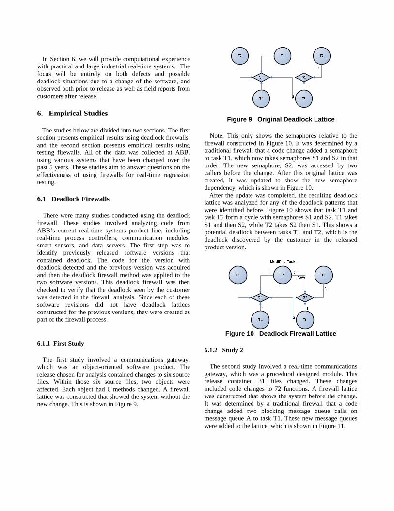
In Section 6, we will provide computational experience with practical and large industrial real-time systems. The focus will be entirely on both defects and possible deadlock situations due to a change of the software, and observed both prior to release as well as field reports from customers after release. 6. Empirical Studies The studies below are divided into two sections. The first section presents empirical results using deadlock firewalls, and the second section presents empirical results using testing firewalls. All of the data was collected at ABB, using various systems that have been changed over the past 5 years. These studies aim to answer questions on the effectiveness of using firewalls for real-time regression testing. 6.1 Deadlock Firewalls There were many studies conducted using the deadlock firewall. These studies involved analyzing code from ABB’s current real-time systems product line, including real-time process controllers, communication modules, smart sensors, and data servers. The first step was to identify previously released software versions that contained deadlock. The code for the version with deadlock detected and the previous version was acquired and then the deadlock firewall method was applied to the two software versions. This deadlock firewall was then checked to verify that the deadlock seen by the customer was detected in the firewall analysis. Since each of these software revisions did not have deadlock lattices constructed for the previous versions, they were created as part of the firewall process. 6.1.1 First Study The first study involved a communications gateway, which was an object-oriented software product. The release chosen for analysis contained changes to six source files. Within those six source files, two objects were affected. Each object had 6 methods changed. A firewall lattice was constructed that showed the system without the new change. This is shown in Figure 9.
Figure 9 Original Deadlock Lattice Note: This only shows the semaphores relative to the firewall constructed in Figure 10. It was determined by a traditional firewall that a code change added a semaphore to task T1, which now takes semaphores S1 and S2 in that order. The new semaphore, S2, was accessed by two callers before the change. After this original lattice was created, it was updated to show the new semaphore dependency, which is shown in Figure 10. After the update was completed, the resulting deadlock lattice was analyzed for any of the deadlock patterns that were identified before. Figure 10 shows that task T1 and task T5 form a cycle with semaphores S1 and S2. T1 takes S1 and then S2, while T2 takes S2 then S1. This shows a potential deadlock between tasks T1 and T2, which is the deadlock discovered by the customer in the released product version.
Figure 10 Deadlock Firewall Lattice
6.1.2 Study 2 The second study involved a real-time communications gateway, which was a procedural designed module. This release contained 31 files changed. These changes included code changes to 72 functions. A firewall lattice was constructed that shows the system before the change. It was determined by a traditional firewall that a code change added two blocking message queue calls on message queue A to task T1. These new message queues were added to the lattice, which is shown in Figure 11.

Figure 11 Deadlock Firewall Lattice
The firewall analysis shows that task T1 now both sends and receives on message queue A. Since both the message queue send and receive operations are blocking, this situation leads to a message queue deadlock, as described in Section 5.4. This problem was detected in the field by customers on this software version and reported to ABB.
6.1.3 Study 3 The third study involved another communications module, which was also a procedurally designed module. This release contained 22 changed files, which contained 41 modified functions. A firewall lattice was constructed that shows the system before the change. It was determined by a traditional firewall analysis that tasks T1 and T2 now use a blocking message queue send. The new message queues were added to the graph; the results of the firewall are shown in Figure 12.
T2
T1
T3
T4
T5
Message Queue A
Message Queue A
Message Queue B
Message Queue B
Message Queue C
Message Queue C
Message Queue D
Figure 12 Deadlock Firewall Lattice
The firewall analysis shows that task T1 sends a message to task T3 via message queue A. Then task T3 sends a message to task T4 on message queue B. After that, task T4 sends a message to task T1 on message queue C. This shows a cyclical deadlock, as described in Section 5.4. This cyclical deadlock was the same deadlock detected by customers in the field and reported to ABB in this software version.
6.1.4 Study 4 The final case study involved using the deadlock firewall analysis on a new piece of changed software. This software had passed all of its unit, integration, regression, and systems tests and was certified as ready for release by
the test department. This new software had 93 files modified, including 112 functions. The deadlock firewall analysis was conducted and yielded the firewall lattice shown in Figure 13.
Figure 13 Firewall Deadlock Lattice
This lattice shows that task T1 sends a message to task T2 on message queue A. Then task T2 sends signal 1 to task T3 and then waits for signal 2 from T3. Task T3 sends a message to T1 on message queue B, and also signals back to task T2. This is a cyclical deadlock case using both signals and message queues. As soon as any one message queue is full, all three tasks will have deadlock. This deadlock was successfully detected by the firewall method, and a major defect was detected prior to release of the software. In addition, three other deadlock conditions were detected, Two of the three dealt with message queue additions, as discussed in study 2, and the other dealt with a more traditional semaphore deadlock. These lattices are not shown here, as they are similar to the above studies.
6.1.5 Summary of Deadlock Firewalls The above case studies show the effectiveness of the deadlock firewall for real-time systems. The first three deadlocks above were detected by customers in the field after installing the new software. The fourth was detected before release, saving a major product defect from being released. These deadlocks were not detected in any testing that was conducted at ABB, including long term stress testing. All of the above deadlocks were added after the first release of the software, due to other customer reported problems. This shows that deadlock can be added quite frequently to minor, incremental software builds. The first three deadlocks caused ABB over 15 man weeks each to debug, fix, test, and re-release. In the meantime, all customers had to use the previous software release, which in some cases did not have the features they needed. These deadlock defects were a major problem for ABB.
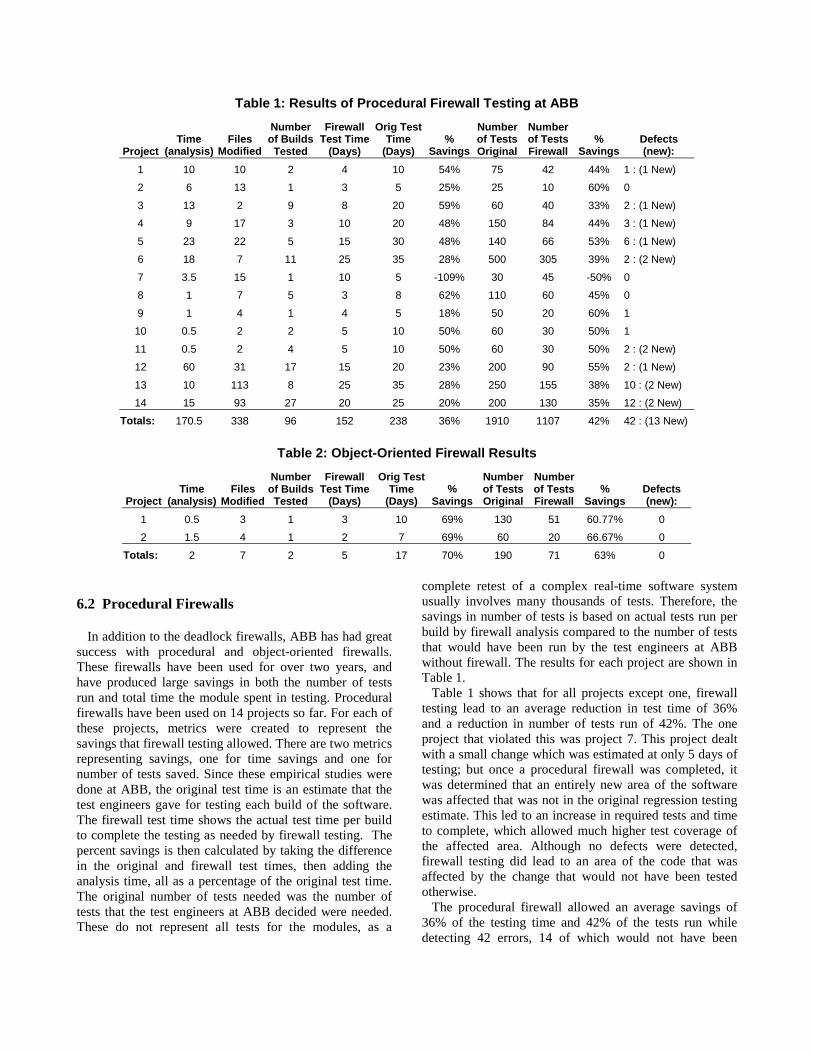
Table 1: Results of Procedural Firewall Testing at ABB
Project Time
(analysis) Files
Modified
Number of Builds Tested
Firewall Test Time
(Days)
Orig Test Time
(Days) %
Savings
Number of Tests Original
Number of Tests Firewall
% Savings
Defects (new):
1 10 10 2 4 10 54% 75 42 44% 1 : (1 New)
2 6 13 1 3 5 25% 25 10 60% 0
3 13 2 9 8 20 59% 60 40 33% 2 : (1 New)
4 9 17 3 10 20 48% 150 84 44% 3 : (1 New)
5 23 22 5 15 30 48% 140 66 53% 6 : (1 New)
6 18 7 11 25 35 28% 500 305 39% 2 : (2 New)
7 3.5 15 1 10 5 -109% 30 45 -50% 0
8 1 7 5 3 8 62% 110 60 45% 0
9 1 4 1 4 5 18% 50 20 60% 1
10 0.5 2 2 5 10 50% 60 30 50% 1
11 0.5 2 4 5 10 50% 60 30 50% 2 : (2 New)
12 60 31 17 15 20 23% 200 90 55% 2 : (1 New)
13 10 113 8 25 35 28% 250 155 38% 10 : (2 New)
14 15 93 27 20 25 20% 200 130 35% 12 : (2 New)
Totals: 170.5 338 96 152 238 36% 1910 1107 42% 42 : (13 New)
Table 2: Object-Oriented Firewall Results
Project Time
(analysis) Files
Modified
Number of Builds Tested
Firewall Test Time
(Days)
Orig Test Time
(Days) %
Savings
Number of Tests Original
Number of Tests Firewall
% Savings
Defects (new):
1 0.5 3 1 3 10 69% 130 51 60.77% 0
2 1.5 4 1 2 7 69% 60 20 66.67% 0
Totals: 2 7 2 5 17 70% 190 71 63% 0
6.2 Procedural Firewalls In addition to the deadlock firewalls, ABB has had great success with procedural and object-oriented firewalls. These firewalls have been used for over two years, and have produced large savings in both the number of tests run and total time the module spent in testing. Procedural firewalls have been used on 14 projects so far. For each of these projects, metrics were created to represent the savings that firewall testing allowed. There are two metrics representing savings, one for time savings and one for number of tests saved. Since these empirical studies were done at ABB, the original test time is an estimate that the test engineers gave for testing each build of the software. The firewall test time shows the actual test time per build to complete the testing as needed by firewall testing. The percent savings is then calculated by taking the difference in the original and firewall test times, then adding the analysis time, all as a percentage of the original test time. The original number of tests needed was the number of tests that the test engineers at ABB decided were needed. These do not represent all tests for the modules, as a
complete retest of a complex real-time software system usually involves many thousands of tests. Therefore, the savings in number of tests is based on actual tests run per build by firewall analysis compared to the number of tests that would have been run by the test engineers at ABB without firewall. The results for each project are shown in Table 1. Table 1 shows that for all projects except one, firewall testing lead to an average reduction in test time of 36% and a reduction in number of tests run of 42%. The one project that violated this was project 7. This project dealt with a small change which was estimated at only 5 days of testing; but once a procedural firewall was completed, it was determined that an entirely new area of the software was affected that was not in the original regression testing estimate. This led to an increase in required tests and time to complete, which allowed much higher test coverage of the affected area. Although no defects were detected, firewall testing did lead to an area of the code that was affected by the change that would not have been tested otherwise. The procedural firewall allowed an average savings of 36% of the testing time and 42% of the tests run while detecting 42 errors, 14 of which would not have been

detected under the previous testing method. These data show that firewall testing allows the tester to understand what area of the software changed and what other parts of the software are affected by that change. This leads to more efficient software testing with fewer wasted tests. No additional errors were detected by the customer on the above software releases that were due to the changes in these releases to date. There were additional defects found, but none were regression or unit test failures. These were pre-existing defects that were created in the original release. 6.3 Object-Oriented Firewalls In addition to procedural firewalls, ABB has used the object-oriented firewall on two software releases. The same metrics and format were used for the object-oriented firewall as for the procedural firewall. These results are shown in Table 2. Table 2 shows that using the object-oriented firewall led to a savings of 70% on total test time and 63% on number of tests run. These numbers are high due to the fact that only two releases were used and both releases were for the same product. In addition, no defects were detected in testing. This was due to the simplicity of the changes in the software. No additional errors were detected in these releases after shipment to the customers to date. 6.4 Global Variable Firewalls ABB has also used global variable firewalls on three software releases. For each of these releases, it was determined that a global variable was defined in a new way. This means that an existing global variable was used, but a new value was assigned to it. This led to a firewall of all uses and definitions of the global variable throughout the software. For the three software releases that used the global variable firewall, no errors were detected. In addition, after over three years in the field, no customers have detected any errors due to global variables. 7. Related Work The notion of deadlock was identified as early as 1972 by Rick Holt [12], where he provided necessary and sufficient conditions for its identification, and also characterized it as a directed cycle in a wait-for digraph. In 1973, Clarence Ellis [13] proved theoretically that as the number of processes and resources increase in a computer system, the probability (or rate of) deadlock increases, although it may still rarely occur. In 1980, Tiko Kameda provided some testing guidelines to achieve deadlock-free computer systems [14].
Other technologies have been used to detect deadlock or guarantee deadlock-free software. For example, in 1990 Dillon [15] used axiomatic specifications and symbolic execution to generate verification conditions to demonstrate absence of deadlock and other safety properties in Ada tasking programs. More recently, model checking has also been used to detect deadlock. In 1995, Mandrioli et. al. [16] used temporal logic to address testing of timing constraints. In 1998, A. En-Nouaary et. al. utilized a state characterization method called the Timed Wp-method to generate tests for real-time systems [17]. In 2001, these same authors presented an extensive real-time fault model to which the Timed Wp-method could be applied [18]. More recently, R. Cordell-Oliver described an alternate finite-state model to test for timing problems in real-time systems [19]. However, more consistent with the theme of this paper, in 2003, Sean Beatty entitles his paper “Where Testing Fails”, and addresses the problems of stack overflows, race conditions and deadlocks [20]. Although some researchers recommend that practitioners not try to detect unlikely potential deadlocks, he recommends the easiest way to avoid them is to use the following design guidelines: • Threads should have no more than one resource
locked at any time. • A thread completely allocates all its needed resources
before it begins execution. • Threads that acquire multiple resources must look
(and release) them in a system wide preset order. This is similar to our approach, where in regression testing we identify potential deadlocks, and ask our software engineers to redesign, avoiding such deadlocks. Beatty also mentions the problem of message passing deadlocks. Also in 2003, Gertrude Levine identified five different deadlock situations, explaining that this has caused problems for both researchers and practitioners when they confuse these different types of deadlock [21]. There has not been much discussion of the need for and consequences of not performing regression testing of modified real-time systems. In 1986, Hassan Gomaa investigated incremental development of real-time systems, and subsequent integration testing [22]. More recently in 2001, Thane et. al. has also recommended integration testing of real-time systems [23].
8. Conclusions and Future Research At ABB, we found that serious problems were being delivered in the real-time software to the customers primarily because of last minute changes. There were many different sources of these problems; we discovered deadlock due to three different mechanisms: tasks and semaphores, tasks and message queues, and task interactions, as well as other types of software defects.

Firewalls were developed for each of these problem sources; these firewalls were very effective in detecting these problems, and at lower cost, since we only systematically searched for defects directly related to the modified areas of the system. In future research, we want to apply firewalls to two other sources of problems: GUI testing and memory leaks due to incremental changes in real-time systems. Since we have already worked out the testing firewall details for GUI systems, it is only a matter of applying this at ABB. For memory leaks, however, this is a new research problem that we have not yet examined. Another area of research is to see if there is any way to combine these firewalls, in the sense that we can share firewall resources or code, so as to reduce the effort to construct all of these firewalls in the presence of incremental change. References [1] Hareton Leung and Lee White, “A Study of Integration Testing and Software Regression at the Integration Level”, Proc. of Conf. on Software Maintenance, pp 290-301, San Diego, 1990. [2] John Bible, Gregg Rothermel and David Rosenblum, “A Comparative Study of Course- and Fine-Grained Safe Regression Test-Selection Techniques”, ACM Trans. on Software Engineering and Methodology, Vol. 10, No. 2, pp 149-183, April 2001. [3] D. Kung, J. Gao, P. Hsia, F. Wen, Y. Toyoshima and C. Chen, “Class Firewall, Test Order and Regression Testing of Object-Oriented Programs”, J. of Object-Oriented Programming, Vol. 8, No. 2, pp 51-65, May 1995. [4] D. Kung, J.Gao, P. Hsia, F. Wen, Y. Toyoshima and C. Chen, “Change Impact Identification in Object-Oriented Software Maintenance”, Proc.of Int. Conf. on Software Maintenance, pp 202-211, Victoria, B. C., Canada, 1994. [5] Lee White and Khalil Abdullah, “A Firewall Approach for the Regression Testin of Object-Oriented Software”, Software Quality Week, San Francisco, May 1997. [6] Lee White, Husain Almezen and Shivakumar Sastry, “Firewall Regression Testing of GUI Sequences and Their Interactions”, Proc. of Int. Conf. on Software Maintenance, pp 398-409, Amsterdam, Sept. 2003. [7] Hareton Leung and Lee White, “Insights into Testing and Regression Testing Global Variables”, J. of Software Maintenance, Vol 2, No. 4, pp 209-222, Dec. 1991. [8] Lee White and Hareton Leung, “A Firewall Concept for both Control Flow and Data Flow in Regression Integration Testing”, Proc. of Conf. on Software Maintenance, pp 262-271, Orlando, FL, 1992. [9] Khalil Abdullah, Jim Kimble and Lee White, “Correcting for Unreliable Regression Integration Testing”, Proc. of Int. Conf. on Software Maintenance, pp 232-241, Nice, France, 1995. [10] A. M. Memon, M. E. Polack and M. L. Soffa, “Hierarchical GUI Test Case Generation Using Automated Planning”, IEEE Trans. on Software Engineering, SE-27(2), pp 144-155, 2001. [11] Lee White, Husain Almezen and Nasser Alzeidi, “User-Based Testing of GUI Sequences and Their Interactions”, Proc.
of Int. Symp. on Software Reliability Engineering, pp 54-63, Hong Kong, Nov. 2001 [12] R. C. Holt, “Some Deadlock Properties of Computer Systems”, ACM Computing Surveys, Vol. 4, No. 3, pp 179-196, Sept. 1972. [13] Clarence Ellis, “On the Probability of Deadlock in Computer Systems, ACM SIGOPS Operating Systems Review, pp 88-95, Vol. 6, Nos. 1-2, June 1973. [14] Tiko Kameda, “Testing Deadlock-Freedom of Computer Systems”, Journal of the ACM, Vol 27, No. 2, pp 170-280, 1980. [15] Laura K. Dillon, “Verifying General Safety Properties of Ada Tasking Programs”, IEEE Trans. on Software Engineering, SE-16(1), pp 51-63, Jan. 1990. [16] Dino Mandrioli, Sandrio Morasca and Angelo Morzenti, “Generating Test Cases for Real-Time Systems from Logic Specifications”, ACM Trans. on Computer Systems,Vol. 13, No. 4, pp 365-398, Nov. 1995. [17] A. En-Nouaary, R. Dssouli, F. Khendek and A. Elqortobi, “Timed Test Cases Generation Based on State Characterisation Technique”, Proc. 19th IEEE Real-TimeSystems Symp. (RTSS ’98), pp 1023-1038, Dec. 1998. [18] A. En-Nouaary, R. Dssouli and F. Khendek, “Timed Wp-Method: Testing Real Time Systems”, IEEE Trans. on Software Eng., Vol. 28, No. 11, pp 1023-1038, Nov. 2002. [19] Rachel Cardell-Oliver, “Conformance Test Experiments for Distributed Real-Time Systems”, Int. Symp. on Systems Testing and Analysis (ISSTA-02), pp 159-163, July, 2002. [20] Sean Beatty, “Where Testing Fails”, Embedded Systems Programming, pp 36-41, Aug. 2003. [21] Gertrude Levine, “Defining Deadlock”, ACM SIGOPS Operating Systems Review, Vol. 37, No. 1, pp 54-64, Jan. 2003. [22] Hassan Gomaa, “Software Development of Real-Time Systems”, Comm. of ACM, Vol. 29, No. 7, pp 657-668, July 1986. [23] Henrik Thane, Anders Pettersson and Hans Hansson, “Integration Testing of Fixed Priority Scheduled Real-Time Systems”, IEEE Real-Time Embedded System Workshop, pp 1-9, Dec. 2001.