table of content issue n° 42 - esarda.jrc.ec.europa.eu · esarda bulletin, no. 42, november 2009 1...
TRANSCRIPT

ISSN 0392-3029
Number 42November 2009
ESARDA is an association formed to advance and harmonize research and development for safeguards. The Parties to the association are:Areva, FranceATI, AustriaBNFL, United KingdomCEA, FranceCNCAN, RomaniaEDF, FranceENEA, ItalyEuropean CommissionFZJ, GermanyHAEA, HungaryIKI, HungaryIRSN, FranceMITyC, SpainNRPA, NorwaySCK/CEN, BelgiumSellafield Ltd, United KingdomSFOE, SwitzerlandSpringfields Fuels Limited, United KingdomSSM, SwedenSTUK, FinlandUKAEA, United KingdomVATESI, LithuaniaWKK, Germany
EditorC. Versino on behalf of ESARDAEC, Joint Research CentreT.P. 210I-21020 Ispra (VA), ItalyTel. +39 0332-789603, Fax. +39 [email protected]
Editorial CommitteeB. Autrusson (IRSN, France)K. Axell (SSM, Sweden)H. Böck (ATI, Austria)J-L Martins (EC, TREN, Luxembourg)P. Peerani (EC, JRC, IPSC, Italy)A. Rezniczek (Uba-GmbH, Germany)B. Richter (FZJ, Germany)F. Sevini (EC, JRC, IPSC, Italy)J. Tushingham (NNL, United Kingdom)C. Versino (EC, JRC, IPSC, Italy)
Scientific and technical papers submittedfor publication are reviewed by the EditorialCommittee.
Manuscripts are to be sent to the Editor following the ‘instructions for authors’ available on the ‘Bulletin’ page of the ESARDA website.Photos or diagrams should be of high quality.
Accepted manuscripts are published free of charge.
N.B. Articles and other material in ESARDA.Bulletin do not necessarily present the views or policies of ESARDA nor of the European Commission.
ESARDA Bulletin is published jointly by ESARDA and the Joint Research Centre of theEuropean Commission.It is distributed free of charge.
The publication is authorized by ESARDA.
© Copyright is reserved, but part of this publica-tion may be reproduced, stored in a retrieval system, or transmitted in any form or by any means, mechanical, photocopy, recording, or otherwise, provided that the source is properlyacknowledged.
Cover designed by N. BährEC, JRC, Ispra, Italy
Printed by IMPRIMERIE CENTRALE – Luxembourg
Table of Content issue n° 42Editorial
Special Issue on Non Destructive Analysis .............................................................. 1P. Peerani
Scientific articles
ESARDA Multiplicity Benchmark Exercise - Phase III and IV .................................. 2 P. Peerani, M. Swinhoe, A-L. Weber, L. G. Evans
A Good Practice Guide for the use of Modelling Codes in Non Destructive Assay of Nuclear Materials ......................................................................................... 26 P.M.J. Chard (Editor)

ESARDA BULLETIN, No. 42, November 2009
1
Editorial
In June 2006, the ESARDA Bulletin published as Issue number 34 the first of the Bulletin’s Special Issues. Special Issues are published occasionally, in addition to the two regular Bulletins published per year, and have a monographic character, being the entire number dedicated to a specific and single topic.
The first Special Issue was dedicated to NDA and contained the final report of the ESARDA Multiplicity Benchmark (at that time dealing with phases I and II). After three years we are back with a Special Issue entirely dedicated to two products of the ESARDA NDA Working Group:
• thereportoftheIIIandIVphasesoftheESARDAMultiplicitybenchmark;
• theGoodPracticeGuidefortheuseofModellingCodesinNonDestructiveAssayofNuclearMaterials.
The first paper describes the continuation of the project that made the subject of the previous Special Issue. Benchmarking is a common procedure in applied science in order to assess and validate methodologies, techniques or components (either instruments or software). The ESARDA Multiplicity Benchmark had a two-fold goal:
• testandvalidateMonteCarlocodesinthesimulationofneutronmultiplicitycounters;
• testandvalidateLIST-modedataacquisitionsoftwarefortheprocessingoftime-stampedpulsetrains.
For this reason, already at the initial step the benchmark had been split in two phases: one aiming to compare fullMonteCarlomodellingofaneutronmultiplicitysystem,thesecondaimingtocomparedataprocessingcodes for the analysis of acquired LIST-mode data. At the time of the first exercise launched in 2003, LIST-mode acquisition system were still under development, so the first exercise was focussed to a series of theoretical cases:sotheMonteCarlosimulationswerebenchmarkedagainsttheoreticalpoint-modelmathematicalsolu-tionsandtheprocessingcodeswereappliedtosyntheticpulsetrainsproducedbyMonteCarlosimulations.
When the first hardware developments were completed at some research laboratories, the first neutron counting systems with LIST-mode data acquisition become available and the NDA working group spon-soredaseriesofexperimentalcampaignsperformedduring2006and2007atthePERLAlaboratoryofJRCto compare some systems. These campaigns made available a set of experimental data that were used asabasisforthecontinuationoftheexercise.TheIIIandIVphasesofthemultiplicitybenchmarkconsistrespectively in thecomparisonof fullMonteCarlosimulationsandLIST-modepulse trainanalysiswith experimental data. The results of this exercise make the subject of the report in this Bulletin.
Thesecondpaperfocusesonasubjectpartlyincommonwiththepreviousone,MonteCarlosimulation.This technique has become more and more frequently used as a complementary tool in NDA measure-ments, in particular replacing experimental calibration when suitable reference material are not available. The introduction of numerical calibration in safeguards procedures had initially to win the reluctance of many sceptics, but an extensive effort of validation (also through several benchmarks organised by the ESARDA NDA working group) and the success of the first trial cases allowed finally to have this technique accepted by IAEA and Euratom.
OnceMonteCarlobecameastandardtechnique,thenuclearsafeguardscommunityrealisedtheneedtoestab-lishcommonandclearrulesontheapplicationofMonteCarlomodelling.InparticulartheIAEAstimulatedtheNDAworkinggrouptodevelopagoodpracticeguide(GPG)innumericalsimulationonasimilarbasisofGPG’sused in the other (experimental) measurement techniques. The document presented in this Bulletin results from thecontributionsofseveralMonteCarloexpertsoftheNDAworkinggroupandprovidesasetofrecommenda-tions of best practices in the application of numerical simulation and modelling of NDA techniques.
Special Issue on Non Destructive AnalysisP. PeeraniEuropean Commission, Joint Research Centre

ESARDA BULLETIN, No. 42, November 2009
2
ESARDA Multiplicity Benchmark Exercise – Phases III and IVP. Peerani1, M. Swinhoe2, A-L. Weber3, L. G. Evans4
1. European Commission, Joint Research Centre, IPSC – Ispra (VA), Italy2. Institut de Radioprotection et Surete Nucleaire, Fontenay-aux-Roses, France3. N-1, Safeguards Science and Technology Group, LANL – Los Alamos (NM), USA4. University of Birmingham, Canberra – Meriden (CT), USAE-mail: [email protected]
Abstract
In 2003 the ESARDA NDA working group launched a benchmark exercise in order to compare the dif-ferent algorithms and codes used in the simulation of neutron multiplicity counters. The results of the 1st and 2nd phase of the ESARDA Multiplicity Bench-mark, based on synthetic cases, have been pub-lished in the ESARDA Bulletin number 34. Notwith-standing the satisfactory conclusion that all the algorithms developed by the different participants in the first two phases and used to analyse the pulse trains have proven to be satisfactory, the working group felt that an extension to real experimental cases would have added a supplementary value to the exercise that brought to the organisation of phases III and IV. This paper summarises the out-comes of the benchmark, whose full report will soon be made available on the ESARDA Bulletin.
Keywords: NDA, neutron counting, neutron multi-plicity,MonteCarlo.
1. Rationale
In 2003 the ESARDA NDA working group launched a benchmark exercise in order to compare the dif-ferent algorithms and codes used in the simulation of neutron multiplicity counters. In order to derive the maximum amount of information and at the same time to allow a large participation, the work-ing group decided to split the exercise into two parts with two participation levels: a full simulation exercise where participants were asked to compute the count rates starting from the basic technical specifications and/or a partial exercise involving the processing of the pulse trains produced by a single laboratory. The results of participants performing the entire exercise enabled a comparison among thedifferentMonteCarlocodesforthesimulationof neutron multiplicity counters. The results of the partial exercise help to test the available algorithms
for pulse train analysis and to derive some impor-tant information about the models applied for dead-time correction. The results of the 1st and 2nd phase of the ESARDA Multiplicity Benchmark have been published elsewhere [1, 2].
All the cases run in the first two phases of the benchmark were theoretical. So the conclusions derived had to be considered as a relative behav-iour of the different models, techniques and codes. Notwithstanding the satisfactory conclusion that all the algorithms developed by the different partici-pants in the first two phases and used to analyse the pulse trains have proven to be satisfactory, the working group felt that an extension to real experi-mental cases would add value to the exercise.
First of all it would provide a further validation to the MonteCarlocodessuchasMCNPX,MCNP-PTAorMCNP-Polimiinthespecificfieldofneutroncorre-lations. In fact to our knowledge, there has been no othercaseofabenchmarkcomparingMonteCarloto experiments on neutron correlations, except the previous ESARDA exercise and even in that case the comparison was limited to Reals (or Doubles) counting [3]. A complete assessment with compari-son of calculated and measured Singles, Doubles and Triples would be accomplished through the 3rd phase of the ESARDA Multiplicity Benchmark.
A more practical consideration brings us to the jus-tification of the 4th phase. Nowadays most of the neutron counting systems is based on feeding a train of TTL logic pulses into a neutron analyser per-forming the time correlation analysis. In future these systems could be replaced by the introduction of time-stamped data acquisition cards that replace the logical pulse by a digital time stamp (LIST mode acquisition). These digital pulse trains could be di-rectly fed to an acquisition computer and processed by software, without further need for an additional hardware component, such as an (ordinary or Mul-
Scientific articles
ESARDA BULLETIN, No. 42, November 2009
3
tiplicity) Shift Register Analyser. This could be the future major development in practical neutron cor-relation analysis, given data transfer rates, storage and analysis criteria can be met. There are potential secondary benefits: e.g. more robust monitoring of thestateofthehealthoftheequipment;thepoten-tial for continued operation with revised calibration parametersgivenfailureofasub-setofdetectors;accesstoalternativeanalysismethods;acompleterecordof thedata; refined fault findingcapabilityetc. The programs developed by the participants to the 2nd phase of the ESARDA Multiplicity Bench-mark can be used directly and without any modifi-cation to process the digital pulse trains produced by experimental measurements performed in LIST mode. The main aim of this exercise is to test and validate the LIST mode operation of neutron multi-plicity counters against the established practice.
2. Description of the exercise
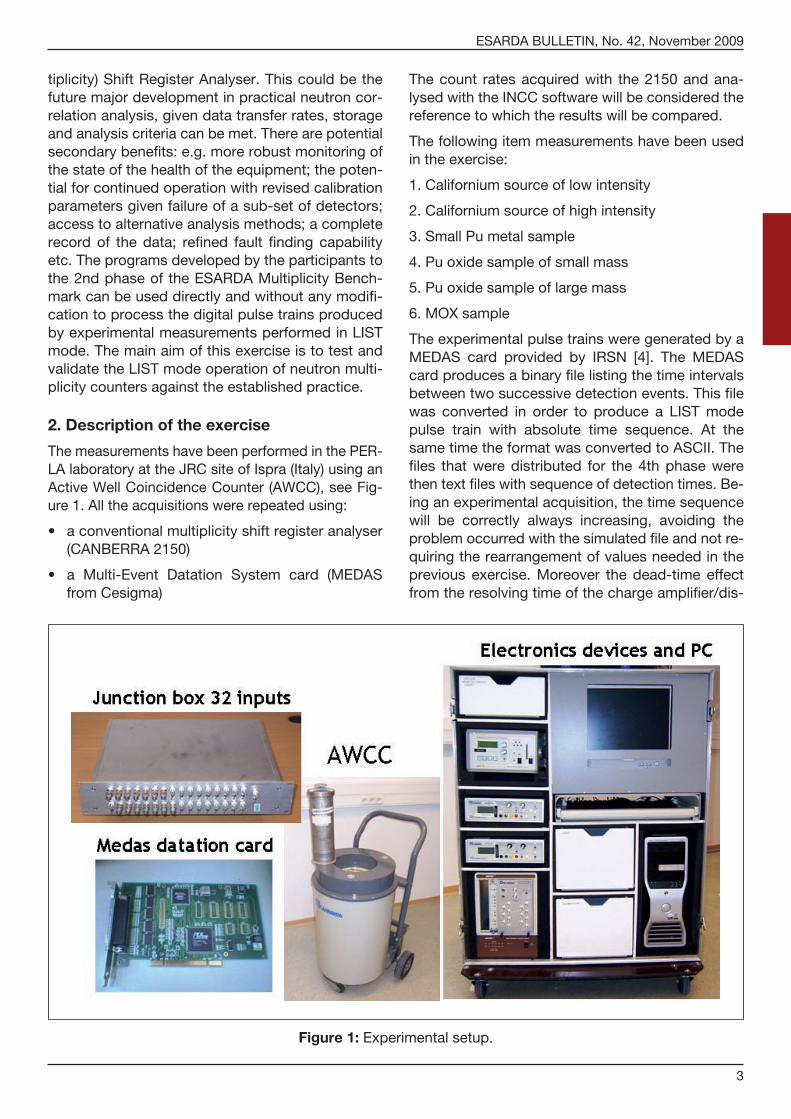
ThemeasurementshavebeenperformedinthePER-LAlaboratoryattheJRCsiteofIspra(Italy)usinganActiveWellCoincidenceCounter(AWCC),seeFig-ure 1. All the acquisitions were repeated using:
• aconventionalmultiplicityshiftregisteranalyser(CANBERRA2150)
• a Multi-Event Datation System card (MEDASfromCesigma)
Thecount ratesacquiredwith the2150andana-lysedwiththeINCCsoftwarewillbeconsideredthereference to which the results will be compared.
The following item measurements have been used in the exercise:
1.Californiumsourceoflowintensity
2.Californiumsourceofhighintensity
3.SmallPumetalsample
4.Puoxidesampleofsmallmass
5.Puoxidesampleoflargemass
6.MOXsample
The experimental pulse trains were generated by a MEDAS card provided by IRSN [4]. The MEDAS card produces a binary file listing the time intervals between two successive detection events. This file was converted in order to produce a LIST mode pulse train with absolute time sequence. At the sametimetheformatwasconvertedtoASCII.Thefiles that were distributed for the 4th phase were then text files with sequence of detection times. Be-ing an experimental acquisition, the time sequence will be correctly always increasing, avoiding the problem occurred with the simulated file and not re-quiring the rearrangement of values needed in the previous exercise. Moreover the dead-time effect from the resolving time of the charge amplifier/dis-
Figure 1: Experimental setup.
ESARDA BULLETIN, No. 42, November 2009
4
criminator boards and subsequent stages of elec-tronic processing is embedded in the measurement chain, so the participants were not asked to remove counts in order to simulate dead-time effects.
3. Specifications for the pulse train generation
ThedetectorusedwasanActiveWellCoincidenceCounter (AWCC) in fastconfiguration (Cd liner in-side the cavity) with both disks removed (cavity height35cm)[5].Thiscorrespondstothespecifi-cation of the one used in the 1st phase avoiding the participants the effort to develop a new detector model. Only the samples had to be modelled ac-cording to the detailed description provided below.
3.1. Case 1 – Cf source of low intensity
Thiscase refers to themeasurementofaCf-252sourceplacedat the centreof theAWCCcavity.Geometrically the source is a very small piece of metal wire and to all effects can be considered point-like. It is contained in a cylindrical stainless steel capsule with an external radius of 0.4 cm, height of 1 cm and wall thickness of 0.13 cm. The intensityofthesource(6005-NC)wascertifiedbyNPLandafterdecaycorrectionitresultstobe3781n/s at the measurement date (with a 1-sigma uncer-tainty of about 1%).
3.2. Case 2 – Cf source of high intensity
The case refers to a geometrical configuration iden-tical to case 1. The only difference is the intensity of thesource (6001-NC) thatwas497200n/sat themeasurement date (with a 1-sigma uncertainty of about 1%).
3.3. Case 3 – Pu metal sample
The case refers to the measurement of a plutonium metal sample (PERLA-211), indeed a PuGa alloywith1.5%Ga.Thegeometryisathin(0.6mm)met-al disk and an approximate diameter of 3.3 cm. It was placed horizontally at the cavity mid-plane (17.5cmfromthebottom).Theplutoniumcertifiedmasswas9.455g, the isotopiccompositionwas0.13%Pu-238, 75.66%Pu-239, 21.49%Pu-240,1.95%Pu-241and0.77%Pu-242,theAm/Puratiowas0.0186,alldatareferredtoJuly1996.
3.4. Case 4 – Pu oxide sample of small mass
The samplewas thePERLA sample 102, being aPuO2 powder with an estimated density of 2.6 g/cm3 contained in a model-200 container. The plutonium
certifiedmasswas51.455g(59.13gofpowder),theisotopiccompositionwas0.199%Pu-238,70.955%Pu-239, 24.583% Pu-240, 3.288% Pu-241 and0.975% Pu-242, the Am/Pu ratio was 0.0102, alldata referred toNovember1987.Thecontainer isconstituted by two shells: an inner cylinder in AISI-304 stainless steel wrapped in a polyurethane bag (this latter can be neglected in the model), all insert-ed in an outer cylindrical box also in AISI-304 stain-less steel, sealed with steel bolts. A 10-cm high alu-minium spacer was used to place the sample at the centre of the measurement cavity.
3.5. Case 5 – Pu oxide sample of large mass
The sample was the PERLA sample 111, also aPuO2 powder, having the same density and isotopic composition of sample 102, only the total mass and container type change. The plutonium certified masswas999.825g(1148.96gofpowder),alwaysreferred toNovember 1987. The containerwas amodel-1000, similar in shape and composition to the previous one, only having larger dimensions. It wasplacedatthebottomoftheAWCCcavity.
3.6. Case 6 – MOX sample
ThesamplewasthePERLAsampleENEA01.ThisisaMOXpowdercontainedinamodel-2500con-tainer placed at the bottomof the AWCC cavity.ThenetMOXpowdermassis1011.13g,ofwhich675.4gisuraniumand168.151gisplutonium.ThedensityissignificantlylowerthanthePuO2powderand was estimated to be 0.7÷0.9 g/cm3. Uranium enrichment is natural, whereas the plutonium iso-topiccompositionwas0.17%Pu-238,66.54%Pu-239, 28.02% Pu-240, 3.26% Pu-241 and 2.01%Pu-242,theAm/Puratiowas0.0081,datareferredtoDecember1988.
4. Results from full simulations
The scope of this part of the exercise is to have a comparison of the different codes available for the complete simulation of a neutron multiplicity coun-ter. Six laboratories provided results for the full exercise.
The laboratories are more or less the same who participated to the phase 1 and they used the same codes:MCNPXbyLANLandIRSN,MCNP-PTAbyJRC,MCNP-PoliMibyChalmersandUniv.Michi-ganandMCNP+AMtechniquebyIPPE.Anewpar-ticipant, IRSN, provided two sets of results: one withMCNPXwith direct calculation ofmoments,thesecondbygeneratingpulsetrainswithMCNPXand then processing the files with the post-proces-

ESARDA BULLETIN, No. 42, November 2009
5
sor TRIDEN, used also for phase 4. Methodological details have been already described in [1] and will not be repeated here.
a) Zero dead-time
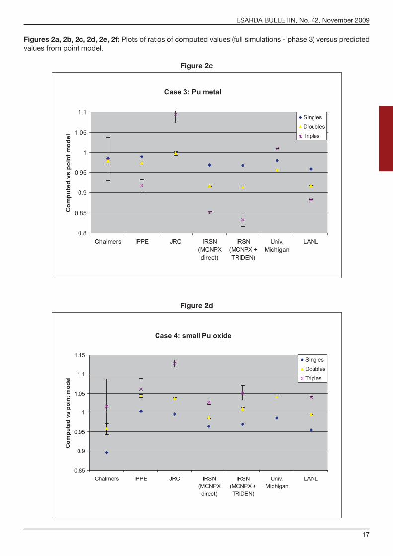
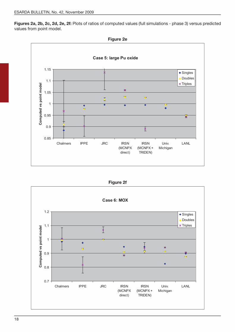
Table 1 shows the comparison of the simulation results in an ideal case of zero dead-time. The quoted uncertainties are purely statistical at 1-sigma level. In this case the calculated values can be compared with the theoretical value com-puted using the point model [6]. The results are also reported in graphical form on plots shown in Figures2a to2f; forpractical reasons in theseplots the point model value was set as reference to 1 even though there is no evidence that this can be assumed as a “true value”. In the axis the participants are labelled from 1 to 6 according to the same order of Table 1.
It is worthwhile to note that comparison to the point model is not trivial, because it requires the knowledge of parameters like the efficiency, the leakage multiplication and the gate utilisation factors. The Pu sources are confounded by(alpha,n) neutrons with a different energy distri-bution and a finite extent which may violate the strict assumptions of the point model, but more importantly the items were not all measured in the same position so there will be a shift in effi-ciency from the centre to the floor. Some vari-ants of the point model may imply a simple ex-ponential die-away and theAWCC is not trulyideal in that sense. The “reference” values re-ported in Table 1 have been computed applying the point model equations with some simplifica-tions and approximations. The values for effi-ciency and multiplication were derived from the MonteCarlocalculations;thisautomaticallyac-counts for variation of efficiency within the cavity, size and shape of the sample, different energy of neutrons from (alpha,n) and spontaneous fission. The doubles gate fraction was computed assum-ing a single exponential with an approximate die-awaytimeof50μsandthetriplesgatefractionwas assumed to be the square of the doubles gate fraction. The moments of the induced fis-sion multiplicity distributions were taken from fast(1MeV)neutronfission,notfromthermalfis-sion as often used.
The results of the simulations at zero dead-time show an excellent agreement among the differ-ent participants, with standard deviations within a few percent in most of the cases. It is true that all the methods have a common model for the simulationofneutrontransportbasedonMCNP,
but the methods differ on the treatment of time correlations and in any case we always expect some effects linked to the human factor (the way in which the user models the system). Taking all this into account the agreement among the re-sults is satisfying.
Even though there is no clear evidence of strong systematic errors, some clear trends are visible. For instance all the results based on MCNPXtend to be consistently lower than those based onMCNP-Polimi;MCNP-PTAtendstooveresti-mate Triples, whereas IPPE method tends to underestimate them.
Moreover the agreement between simulations, theoretical expectations and measurements are also good. This confirms the applicability of the point model in the cases represented in this exercise.
b) Dead-time effects
The previous data cannot be directly compared with measurements, since measured data are af-fected by dead-time effects. So we have two possibilities, either we correct the measured data in order to derive zero dead-time values or the dead-time effects should be included in the sim-ulation. Dead-time corrected experimental val-ues have been also included in Table 1 and can be compared with the zero dead-time simula-tions there. In this section we have considered the second option.
MCNP-PTAallowsdirectmodellingofdead-timefor each component of the electronic chain (am-plifiersandOR-chainormixer),MCNPXcanpro-duce a pulse train file that can be post-proc-essed by a simulation program that includes dead-time effects (in case of IRSN the TRIDEN software uses a global system dead-time). Both codes apply a paralysable dead-time model. JRCusedadead-timecomponentof1μspereach of the 6 amplifiers and 20 ns for the OR-chain; thiscorrespondstoasystemdead-timeof1000/6+20=187ns,consistentwiththeoneusedbyIRSN(170ns).ThereforeIRSNandJRCprovided as well a set of results that can be di-rectly compared with measured values. This is reported in Table 2.
When comparing simulations with measure-ments, we notice a less close agreement. This can only be marginally attributed to the uncer-tainty introduced by dead-time effects, or the way how the dead-time is modelled. There is certainly some unresolved inconsistency be-tween the model and the reality. This is espe-

ESARDA BULLETIN, No. 42, November 2009
6
cially true for the low count rate cases where the dead-time correction is negligible. This is con-firmed by the comparison of the dead-time cor-rections (obtained by dividing the results of Ta-ble 1 by those of Table 2) shown in Table 3.
By consequence we have to attribute the origin of the discrepancies to modelling and, to a less extent, to the nuclear data used by the two codes. Indeed we have to keep in mind that the PERLAstandardsarecertifiedwithaveryhighprecision in terms of mass and isotopic compo-sition, but much less in terms of their geometri-calproperties.Containersizeisofcourseknown,but there is a large uncertainty on the powder densityofcases4,5and6thatisreflectedonan uncertainty of the filling height and therefore on the actual sample dimensions. This affects quite strongly the multiplication and therefore in-troduces a systematic error that increases with the order of the moments. Especially in case 6 thedensityofMOXpowderisnotknownatall(explaining the strong discrepancies in this case), whereasthedensityofPuO2(assumedtobe2.6g/cm3) has been obtained using some gamma scanning of the containers that allowed us to de-rive the powder filling height with reasonable ac-curacy. A similar consideration applies to case 3 where the sample thickness is not certified.
5. Results from pulse train analysis
The LIST mode files processed from the MEDAS card acquisitions have been distributed to the par-ticipants, who were requested to compute the Sin-gles, Doubles and Triples counting rates for all the pulse trains. For each case 1000-second acquisi-tions were performed, more precisely ten independ-ent acquisitions of 100 seconds. The participants produced the S, D and T count rates (average on the ten short acquisitions) together with their abso-lute uncertainties. Additionally they were requested to provide indicative processing times of the pulse trainstogetherwiththePCcharacteristics.
The same consideration about the methodology ap-plies to phase 4, where the participants used the same tools as in phase 2 and therefore they are fully de-scribed in the final report of the first two phases [1].
All the results are reported in tabular form in Table 4 and graphically in Figures 3a to 3f. Generally the agreement among the different processing codes is extremely good: negligible deviations in Singles (less than 0.1%), agreement within 0.1%-0.4% in Doubles. Nevertheless dispersion up to 4% in Tri-
ples is visible, indicating that the way to compute them is not totally homogeneous.
The values can also be compared to the measured S, D, T with a multiplicity shift register. Indeed it is one of the scopes of the exercise to assess the ca-pability of LIST mode acquisition to correctly collect the measured data in view of a possible alternate technology in time-stamped data acquisition for neu-tron counting applications. Indeed the results show that data acquired with the data acquisition card and processed with all the tested codes agree with the multiplicity shift register data within the statistical uncertainties. We should bear in mind that the shift register measurements and the LIST mode measure-ments were done with the same experimental setup, but sequentially in time. This means that they do not refer exactly to the very same pulse train, but to two sequential pulse trains acquired in identical condi-tions. Also it is possible that the shift register and List Mode units introduce slightly different dead-times. So we can only conclude that they coincide within the statistical uncertainty and no systematic deviations have been revealed. We remind that the “measured” data reported in Table 4 refer to the raw values provided by multiplicity shift register without any correction (neither dead-time nor background).
Observation of the data in Table 4 reveals that the assessment of uncertainties in the mean count rates varies between participants. As reported above, the relative standard deviations in the mean count rates vary up to a maximum of 4% for Triples, however the deviations in the uncertainty estimates them-selves are significantly greater. A deviation of up to 460% has been observed in the calculated uncer-tainties, relative to the measured uncertainties. The greatest dispersion in uncertainty estimates be-tween participants was for the uncertainties in the mean Triples rates for case 2 with the highest source intensity.
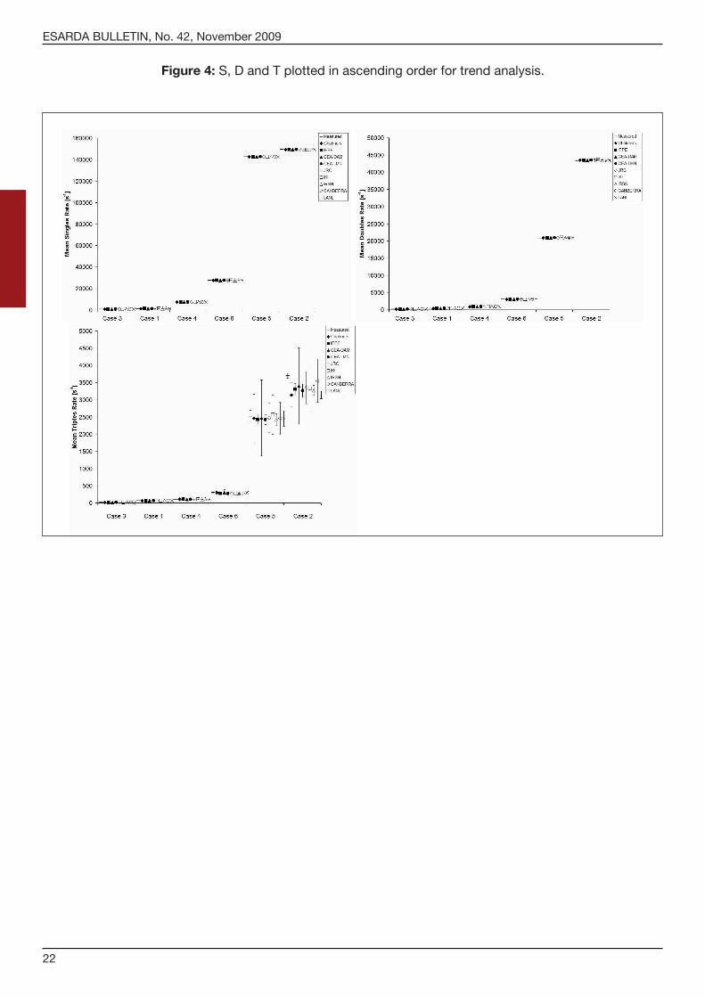
Three summary plots are given in Figure 4 to show the measured Singles, Doubles and Triples count rates, in ascending order of count rate, for each of the six source cases. It is then of interest to plot the Singles, Doubles and Triples rates for each of the cases individually to illustrate trends in the data and the magnitude of differences in the uncertainty esti-mates between participants. The measured and calculated Singles, Doubles and Triples rates have been plotted for each of the six source cases in Fig-ures5a,5band5c,respectively.Cleartrendinginthe distribution of uncertainties can be observed in these three figures. Participant laboratory CEA-DAM had consistently higher uncertainty estimates than other participants. This can be explained by

ESARDA BULLETIN, No. 42, November 2009
7
the fact that reporteduncertainties forCEA-DAMwere quoted as two standard deviations of the mean count rates. It has therefore been deemed necessary to document how uncertainties were cal-culated. All participants were asked to provide a detailed method of how they calculated the uncer-tainties on the Singles, Doubles and Triples rates. Calculation methods from individual participantgroups have been reported in Appendix.
The S, D and T rates from each group have been plotted in ascending order (from lowest to highest) on 3 curves, along with the reported uncertainty values to see if any further trending in the data can be observed. This also provides a visual check as to whether one participant is consistently low or high in reporting uncertainties – see Figure 4.
A further point of interest is the processing time re-quired which varies by more than an order of mag-nitude. This will be partly due to the computer processing power available but there may also be tips and tricks that could benefit the safeguards community, if, as we expect, there is widespread future use of list mode data. For instance IKI processingcodeissystematicallythefastest;thiscould be due to the use of integer mathematics, which is much faster than using floating point num-bers.JRCpost-processingcodehadanevolutionduring the exercise that reduced his running time of more of an order of magnitude, just by optimising theprogramming(compareresultsJRCandJRC-2in Table 4).
6. Conclusions
The results presented here lead to a number of in-teresting and important conclusions. There are two separate topics. The first is the simulation of meas-urementsusingMonteCarlo.Inthisareatheresultsof the different participants are very similar. Howev-er differences do remain. This is in spite of the fact that the basic geometric model was the same in all cases. A close comparison of the input/output files used by the participants will reveal the sources of these differences. The effect of input parameters such as fill height or nuclear data is available in these results and could lead to useful information on theaccuracyofsimulationsforMonteCarlousers.
The second part of the work involved the analysis of pulse trains. In this area also the results from the different participants are very similar. The difference between the results is small for most practical pur-poses. However when one considers that each team was starting from identical pulse trains it seems that further detailed comparison of the algo-
rithms used would be warranted. One free parame-ter in the analysis is the length of the long delay and another difference is how the physical end of the data is treated. Otherwise the results would be ex-pected to be truly identical. A study of the different data treatment algorithms could be used to estab-lish a reference standard for the data analysis.
One outstanding feature of these results is the quoted absolute error. The values appear to vary by an order of magnitude from group to group. This is an important issue that again should be studied by a more detailed comparison of the calculation meth-ods and even definitions of uncertainty used by the different groups. The results could be compared to the values from the shift register electronics and theoretical values. We just underline that from a theoretical point of view the statistical uncertainty of a measurement should not depend on the fact that the acquisition is done using a shift register or LIST mode.
Overall, the results of this exercise show that all participants are capable of good performance for practical purposes. However, comparison of the methods used by the different groups should allow the establishment of more robust analysis tech-niques with more reliable error estimates.
Appendix – calculation of uncertainties
Here we will report the methods used by some of the participants to estimate the uncertainties based on information provided by the authors:
JRC:
The quoted uncertainty is the sample standard de-viations for counting rates computed using the 10 results of the individual runs.
Birmingham/CanberraMethod(L.Evans):
In each of the 6 cases, the MSR analysis was com-pleted for each of the 10 pulse trains. Each of the 10 pulse trains (approximately 100 seconds in length) were further divided into 10 segments of approxi-mately 10 seconds in duration, then 20 cycles of ap-proximately5secondsinduration.Thepurposeofthis segmented pulse train analysis was to enable the estimation of the dispersion in the mean rates, based on replicate counting of an assay item.
The mean S, D and T rates quoted in the spread-sheet were calculated by the following method:
• S,D&Trateswerecalculatedforeachcycle
• AverageS,D&Trateswerecalculatedforeachpulse train by summing rates from each of the cycles and dividing by the number of cycles.

ESARDA BULLETIN, No. 42, November 2009
8
• ThefinalmeanratesquotedforeachsourcearetheaverageoftheS,D&Tratesfromeachofthe 10 pulse trains.
The uncertainty in each of the mean rates is ex-pressed as the standard error, representing the spread in the mean rates over the 10 (or 20 seg-ments as appropriate). Again, the standard error quoted in the final results is an average uncertainty over each of the 10 pulse trains.
CEA-DAM(R.Oddou):
The calculated uncertainties is equal the twice standard deviation of the 10 values
S=mean(Si) (i=1to10)Sabsunc=2*standarddeviation(Si) (i=1to10)The same was done for D and T.
Note: in order to make the results consistent with theotherparticipants,theCEA-DAMresultsreport-ed in Table 4 and in Figures 3 are those provided by the author divided by two.
Chalmers(B.Dahl):
The uncertainty given was calculated as the stand-ard deviation according to the formula
where is the mean value and are the values from the 10 different sets.
IPPE(V.Nizhnik):
Two methods were used: the first estimates count-ing rate random errors based on sample standard deviation upon 10 cycles (pulse-trains). The sec-ond one is based on theoretical standard deviation estimation derived from summarized SR multiplic-ity distribution. For these calculations we used procedures described in [B. Harker, M. Krick: “INCCSoftwareUsersManual”, LA-UR-99-1291(July1998)].
Both methods showed good agreement for Singles and Doubles counting rates, but at the same time, big discrepancy was observed between these two methods for Triples.
References[1] P.Peerani:“ESARDAMultiplicityBenchmarkExercise–Final
report”, ESARDA Bulletin, Nr. 34, June 2006, pages 2-32.
[2] P.Peerani,M.Swinhoe:“ResultsoftheESARDAMultiplicityBenchmarkExercise”,Proc.ofthe47thINMMAnnualMeet-ing, Nashville (TN), 17-20 July 2006.
[3] P.Baeten,M.Bruggeman,P.Chard,S.Croft,D.Parker,C.Zimmerman, M. Looman, S. Guardini: “Results of the ESARDA REALSPredictionBenchmarkExercise”,ESARDABulletin,Nr.31,April2002,pages18-22.
[4] http://gno.cesigma.free.fr/Gb/Accueil/Sommaire.htm
[5] http://www.canberra.com/pdf/Products/Systems_pdf/jcc_51.pdf
[6] N. Ensslin et al.: “Application Guide to Neutron Multiplicity Counting”,LA-13422-M(November1998).

ESARDA BULLETIN, No. 42, November 2009
9
Counting
timeSingles
rateS abs.
unc.Doubles
rateD abs.
unc.Triples
rateT abs.
unc.
Case 1: Cf low intensity
Point model 1170 380.28 68.84
Experimental (DT corrected) 1211 382.64 67.66
ChalmersUniv. 1000 1175 3.85 386.56 4.25 71.66 3.25
IPPE 1000 1147 2.12 362.00 1.34 61.01 0.43
JRC 52000 1167 0.21 376.61 0.13 73.70 0.88
IRSN(MCNPXdirect) 1167 0.47 374.68 0.37 67.34 0.19
IRSN(MCNPX+TRIDEN) 1000 1165 2.20 374.29 1.37 67.69 0.91
Univ. Michigan 1160 376.91 73.64
LANL 1160 0.46 372.48 0.45 66.85 0.21
Relative standard deviation 0.01 0.02 0.07
Case 2: Cf high intensity
Point model 153837 50011 9053
Experimental (DT corrected) 153768 48545 8347
ChalmersUniv. 1000 154692 23.88 51032 238.47 9432 585.63
IPPE 1000 150770 17.83 47602 82.24 8022 219.28
JRC 402 153070 25.73 48880 123.23 8760 363.82
IRSN(MCNPXdirect) 153318 61.33 49240 49.24 8850 24.78
IRSN(MCNPX+TRIDEN) 1000 153282 11.80 49318 49.07 8434 72.57
Univ. Michigan 153572 49786 8656
LANL 151826 60.73 48738 58.49 8747 27.99
Relative standard deviation 0.01 0.02 0.05
Case 3: Pu metal
Point model 724 142.38 16.72
Experimental (DT corrected) 721 129.25 14.29
ChalmersUniv. 1000 713 3.06 139.48 1.59 16.45 0.89
IPPE 1000 716 0.91 138.65 0.85 15.35 0.22
JRC 52000 722 0.17 142.17 0.74 18.31 0.41
IRSN(MCNPXdirect) 701 0.14 130.46 0.09 14.24 0.03
IRSN(MCNPX+TRIDEN) 1000 700 1.51 129.97 0.51 13.93 0.23
Univ. Michigan 708 136.13 16.89
LANL 693 0.03 130.64 0.01 14.76 0.01
Relative standard deviation 0.01 0.04 0.10
Case 4: Pu oxide small mass
Point model 7297 904.87 107.36
Experimental (DT corrected) 7328 919.14 113.83
ChalmersUniv. 1000 6534 5.87 866.51 12.48 109.03 7.85
IPPE 1000 7317 2.83 944.07 4.10 113.96 3.08
JRC 6378 7282 1.40 945.02 1.39 126.93 1.14
IRSN(MCNPXdirect) 7031 6.24 892.64 1.38 110.14 0.62
IRSN(MCNPX+TRIDEN) 1000 7072 3.42 912.41 3.65 112.86 2.22
Univ. Michigan 7196 942.05 136.16
LANL 6962 0.92 901.04 0.61 111.58 0.26
Relative standard deviation 0.04 0.03 0.09
Table 1: Results from (zero dead-time) simulations and comparison with theoretical (point model) values.

ESARDA BULLETIN, No. 42, November 2009
10
Counting
timeSingles
rateS abs.
unc.Doubles
rateD abs.
unc.Triples
rateT abs.
unc.
Case 5: Pu oxide large mass
Point model 147656 23009 4224
Experimental (DT corrected) 146568 23316 4595
ChalmersUniv. 1000 130564 33.01 20957 238.98 4093 546.71
IPPE 1000 146530 16.00 22487 71.05 3814 170.95
JRC 242 147060 31.30 23456 147.31 4802 363.75
IRSN(MCNPXdirect) 146731 28.43 23748 17.39 4474 11.60
IRSN(MCNPX+TRIDEN) 1000 146818 4.38 23650 24.25 3765 36.59
Univ. Michigan 144804 22940 5137
LANL 139974 15.10 21894 17.70 3980 8.90
Relative standard deviation 0.04 0.05 0.12
Case 6: MOX sample
Point model 26157 3411 371.56
Experimental (DT corrected) 27772 3128 348.26
ChalmersUniv. 1000 25719 10.93 3397 37.14 373.18 30.04
IPPE 1000 25504 4.00 3184 10.74 303.24 17.94
JRC 2388 26135 4.60 3414 8.53 397.14 8.44
IRSN(MCNPXdirect) 24784 4.63 3109 1.87 329.09 0.72
IRSN(MCNPX+TRIDEN) 1000 24773 3.95 3124 7.59 348.58 13.53
Univ. Michigan 21552 3123 349.58
LANL 23507 2.50 2991 2.40 336.21 0.80
Relative standard deviation 0.06 0.05 0.09
Table 1: Results from (zero dead-time) simulations and comparison with theoretical (point model) values.

ESARDA BULLETIN, No. 42, November 2009
11
Singles rate Doubles rate Triples rate
Case 1: Cf low intensity
measured 1208.08 380.73 66.62MCNP-PTA 1164.60 374.73 71.96
(C-E)/E -3.6% -1.6% 8.0%
MCNP-Polimi 1157.74 375.63 72.60
(C-E)/E -4.2% -1.3% 9.0%
MCNPX+post-processor 1162.61 372.82 66.65
(C-E)/E -3.8% -2.1% 0.0%
Case 2: Cf high intensity
measured 149338 43374 3695MCNP-PTA 148660 43673 3743
(C-E)/E -0.5% 0.7% 1.3%
MCNP-Polimi 149976 45438 4550
(C-E)/E 0.4% 4.8% 23.1%
MCNPX+post-processor 149145 44398 3734
(C-E)/E -0.1% 2.4% 1.0%
Case 3: Pu metal
measured 720.51 129.09 14.07MCNP-PTA 701.41 133.32 15.07
(C-E)/E -2.7% 3.3% 7.1%
MCNP-Polimi 707.63 135.83 16.65
(C-E)/E -1.8% 5.2% 18.4%
MCNPX+post-processor 698.72 129.50 13.69
(C-E)/E -3.0% 0.3% -2.7%
Case 4: Pu oxide small mass
measured 7313.46 912.24 109.29MCNP-PTA 7267.50 937.93 121.09
(C-E)/E -0.6% 2.8% 10.8%
MCNP-Polimi 7183.27 935.75 130.34
(C-E)/E -1.8% 2.6% 19.3%
MCNPX+post-processor 7059.04 906.40 108.36
(C-E)/E -3.5% -0.6% -0.9%
Case 5: Pu oxide large mass
measured 142622 20873 2519MCNP-PTA 143100 20998 2632
(C-E)/E 0.3% 0.6% 4.5%
MCNP-Polimi 141739 21156 3696
(C-E)/E -0.6% 1.4% 46.7%
MCNPX+post-processor 143143 21499 2053
(C-E)/E 0.4% 3.0% -18.5%
Case 6: MOX sample
measured 27623 3064 301.8MCNP-PTA 25995 3344 344.2
(C-E)/E -5.9% 9.1% 14.0%
MCNP-Polimi 21471 3078 320.3
(C-E)/E -22.3% 0.5% 6.1%
MCNPX+post-processor 24654 3066 303.40
(C-E)/E -10.7% 0.1% 0.5%
Table 2:Comparisonofmeasurementsandsimulationswithdead-timeeffects.

ESARDA BULLETIN, No. 42, November 2009
12
Singles Doubles Triples
Case 1: Cf low intensity
MCNP-PTA 1.002 1.005 1.024
MCNP-Polimi 1.002 1.003 1.014
MCNPX+TRIDEN 1.002 1.004 1.016
Case 2: Cf high intensity
MCNP-PTA 1.03 1.12 2.34
MCNP-Polimi 1.02 1.10 1.90
MCNPX+TRIDEN 1.03 1.11 2.26
Case 3: Pu metal
MCNP-PTA 1.001 1.003 1.016
MCNP-Polimi 1.001 1.002 1.014
MCNPX+TRIDEN 1.002 1.004 1.018
Case 4: Pu oxide small mass
MCNP-PTA 1.002 1.008 1.048
MCNP-Polimi 1.002 1.007 1.045
MCNPX+TRIDEN 1.002 1.007 1.042
Case 5: Pu oxide large mass
MCNP-PTA 1.03 1.12 1.82
MCNP-Polimi 1.02 1.08 1.39
MCNPX+TRIDEN 1.03 1.10 1.83
Case 6: MOX
MCNP-PTA 1.005 1.021 1.15
MCNP-Polimi 1.004 1.015 1.09
MCNPX+TRIDEN 1.005 1.019 1.15
Table 3:Comparisonofdead-timecorrectionfactors.
ESARDA BULLETIN, No. 42, November 2009
13
Counting time
Singles rate
S abs. unc.
Doubles rate
D abs. unc.
Triples rate
T abs. unc.
Time
Case 1: Cf low intensity
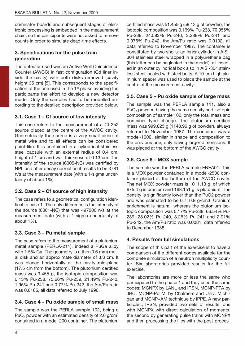
Measured 1247.87 1.58 380.78 0.84 66.65 0.48
ChalmersUniv. 1053.32 1244.42 4.49 382.26 2.94 67.09 2.23 3.4
IPPE 1050.00 1244.44 1.43 381.70 0.77 66.39 0.57 1.0
CEA-DAM 1053.32 1244.34 4.49 381.88 2.43 66.72 2.99 0.5
CEA-LMN 1243.94 1.57 381.90 1.14 66.74 0.75 0.7
AREVA 1040.00 1244.30 4.37 382.07 3.87 72.52 2.74 8.2
JRC 1053.24 1244.40 4.48 381.26 2.94 66.23 2.12 2.0
JRC-2 1053.32 1244.37 4.50 381.80 2.82 66.67 1.98 2.8
IKI 954.90 1243.90 1.10 382.60 1.20 67.30 2.00 1.0
IRSN 1053.29 1244.39 1.42 381.60 0.75 66.35 1.75 5.9
CANBERRA 1053.20 1244.70 4.61 381.32 3.50 66.37 2.51 0.9
Univ. Michigan 1053.30 1244.36 381.96 72.48
LANL 1053.25 1244.39 1.42 382.23 0.92 67.07 0.71 0.8
Rel. stand. dev. 0.000 0.001 0.034
Case 2: Cf high intensity
Measured 149378.13 7.30 43373.58 33.22 3695.29 71.23
ChalmersUniv. 1000.39 149364.24 45.84 43522.80 178.00 3142.29 352.84 4030.0
IPPE 1000.00 149360.00 15.22 43454.00 66.91 3310.80 161.28 34.0
CEA-DAM 1000.39 149362.55 45.87 43522.68 231.62 3403.39 551.33 689.3
CEA-LMN 149364.27 16.74 43470.35 77.52 3266.27 189.99 45.3
AREVA 990.00 149364.15 43.03 43492.82 245.88 3785.99 455.87 972.1
JRC 1000.34 149364.22 45.80 43525.16 286.15 3353.66 469.35 4989.0
JRC-2 1000.38 149364.26 45.87 43513.48 251.58 3328.03 644.65 218.0
IKI 999.06 149364.00 12.00 43543.00 65.00 3334.00 646.00 17.0
IRSN 1000.38 149364.26 14.50 43470.39 64.04 3271.56 144.81 2267.9
CANBERRA 1000.30 149364.63 59.18 43532.54 244.70 3554.16 627.31 1075.0
Univ. Michigan 1000.40 149360.80 43484.06 4053.14
LANL 1000.34 149364.21 14.49 43522.92 55.69 3145.53 112.13 113.0
Rel. stand. dev. 0.000 0.001 0.032
Case 3: Pu metal
Measured 760.288 1.123 129.141 0.566 14.099 0.303
ChalmersUniv. 1269.51 761.16 3.34 130.84 1.68 14.16 0.68 2.5
IPPE 1270.00 761.15 1.06 130.62 0.46 13.95 0.20 0.0
CEA-DAM 1269.51 761.12 3.34 131.07 1.53 14.20 0.65 0.3
CEA-LMN 760.10 1.03 130.42 0.59 14.00 0.28 0.6
AREVA 1000.00 760.10 3.45 130.45 1.57 15.50 0.88 3.4
JRC 1269.42 761.17 3.34 130.62 1.55 14.13 0.48 2.0
JRC-2 1269.51 761.14 3.34 130.86 1.66 14.23 0.72 2.4
IKI 1108.76 760.50 0.90 130.70 0.60 14.40 0.80 1.0
IRSN 1269.48 761.15 1.06 130.68 0.44 13.98 0.19 4.3
CANBERRA 1269.40 761.33 3.09 130.63 1.52 14.16 0.62 1.1
Univ. Michigan 1269.50 761.43 130.68 15.50
LANL 1269.41 761.16 1.06 130.84 0.53 14.16 0.22 0.8
Rel. stand. dev. 0.001 0.001 0.009
Table 4: Results from experimental pulse train processing and comparison with multiplicity shift register measurements.

ESARDA BULLETIN, No. 42, November 2009
14
Counting time
Singles rate
S abs. unc.
Doubles rate
D abs. unc.
Triples rate
T abs. unc.
Time
Case 4: Pu oxide small mass
Measured 7353.24 4.43 912.29 3.76 109.32 2.83
ChalmersUniv. 1070.66 7345.31 11.26 913.10 8.62 110.78 6.96 28.3
IPPE 1070.00 7345.30 3.56 906.72 3.94 106.56 2.55 3.0
CEA-DAM 1070.66 7345.18 11.26 910.12 9.43 110.11 8.22 4.1
CEA-LMN 7345.65 3.09 906.43 3.66 107.00 2.35 2.2
AREVA 1000.00 7345.65 12.16 910.25 10.89 117.06 7.27 29.9
JRC 1070.62 7345.30 11.28 908.96 9.20 108.53 6.17 37.0
JRC-2 1070.66 7345.27 11.25 906.70 6.84 109.61 7.89 11.6
IKI 1053.90 7345.40 2.60 907.40 3.30 110.00 7.70 1.0
IRSN 1070.65 7345.27 3.56 906.65 4.12 106.49 2.66 38.3
CANBERRA 1070.60 7345.47 9.24 908.95 10.54 108.76 6.44 8.0
Univ. Michigan 1070.60 7345.64 907.41 118.75
LANL 1070.61 7345.29 3.57 913.10 2.73 110.78 2.21 3.7
Rel. stand. dev. 0.000 0.003 0.015
Case 5: Pu oxide large mass
Measured 142661.62 16.19 20873.04 40.18 2518.91 175.20
ChalmersUniv. 1001.80 142611.58 33.83 20940.06 255.57 2459.96 702.97 3700.0
IPPE 1000.00 142610.00 10.85 20909.00 63.13 2432.50 142.18 33.0
CEA-DAM 1001.80 142609.95 33.91 20949.26 164.21 2473.05 551.68 630.0
CEA-LMN 142611.03 14.21 20913.85 63.36 2420.11 141.24 44.1
AREVA 1000.00 142611.03 33.80 20931.81 237.37 2911.00 743.75 907.5
JRC 1001.76 142611.49 34.04 20925.37 209.17 2473.20 431.78 4536.0
JRC-2 1001.79 142611.59 33.92 20973.49 108.53 2562.83 566.41 208.0
IKI 1000.84 142611.00 12.00 20987.00 56.00 2568.00 572.00 16.0
IRSN 1001.79 142611.59 10.72 20912.59 67.72 2422.62 171.51 2096.9
CANBERRA 1001.80 142612.12 38.28 20934.08 183.00 2462.23 460.18 916.4
Univ. Michigan 1001.80 141606.60 20776.55 2872.58
LANL 1001.75 142611.47 10.76 20939.33 80.74 2458.78 223.22 104.0
Rel. stand. dev. 0.002 0.002 0.021
Case 6: MOX sample
Measured 27662.76 5.23 3063.97 15.55 301.84 19.31
ChalmersUniv. 1018.88 27658.27 17.35 3082.96 35.38 292.67 47.84 200.0
IPPE 1020.00 27658.00 5.50 3053.40 9.83 276.40 10.37 6.0
CEA-DAM 1018.88 27657.91 17.33 3059.32 18.40 303.23 40.18 31.3
CEA-LMN 27658.42 6.25 3053.55 11.82 274.67 11.99 7.8
AREVA 1000.00 27658.43 18.47 3073.31 35.94 310.16 44.15 118.4
JRC 1018.84 27658.23 17.33 3075.91 26.28 283.85 36.96 224.0
JRC-2 1018.87 27658.24 17.33 3071.09 22.21 294.35 38.00 40.0
IKI 912.89 27661.30 5.50 3071.90 10.60 281.50 37.40 3.0
IRSN 1018.87 27658.24 5.48 3052.45 9.93 276.79 10.75 179.2
CANBERRA 1018.80 27658.48 21.07 3075.86 35.71 283.15 35.56 52.1
Univ. Michigan 1018.90 27657.43 3055.31 315.23
LANL 1018.84 27658.22 5.48 3082.92 11.18 292.69 15.15 14.2
Rel. stand. dev. 0.000 0.004 0.031
Table 4: Results from experimental pulse train processing and comparison with multiplicity shift register measurements.

ESARDA BULLETIN, No. 42, November 2009
15
Participant Contributors Institution
JRC PaoloPeeraniZ. DzbikowiczM. Marin FerrerLuc DechampPascalDransart
EuropeanCommission,JointResearchCentre,IPSC,Ispra,Italy
LANL Martyn SwinhoeSteve Tobin
N-1, Safeguards Science and Technology Group Los Alamos (NM), USA
CANBERRA (Univ.Birmingham)
StephenCroftLouise G. Evans
CANBERRAIndustriesIncMeriden(CT),USA
IPPE Boris RyazanovVladimirNyzhnikValeryBoulanenko
InstituteforPhysicsandPowerEngineering,RMTC,Obninsk,Russia
IRSN Anne-Laure WeberThierry Lambert
Institut de Radioprotection et Sûreté Nucléaire, IRSN/DSMR/SATE, Fontenay-aux-Roses, France
CEA-DAM Raphael Oddou Commissariatal'EnergieAtomique,CEA/DAM,Bruyères-le-Châtel,France
CEA-LMN Anne-CecileRaoux Commissariatàl'EnergieAtomique,DTN/SMTM/LMN,Cadarache,France
ChalmersUniversity Berit Dahl ImrePazsit
Dept. of Nuclear Engineering, ChalmersUniversityofTechnology,Goteborg, Sweden
IKI Janos Bagi Jozsef Huszti
Institute of Isotopes of the Hungarian Academy of SciencesBudapest, Hungary
AREVA Lionel Tondut AREVANC,établissementdeLaHague,Baumont Hague, France
Univ. Michigan SaraPozziShaunClarkeEric Miller
University of Michigan, Dept. Nucl. Eng.,Ann Arbor (MI), USA
Table 5:Contributorstothe“ESARDAMultiplicityBenchmarkExercise”.

ESARDA BULLETIN, No. 42, November 2009
16
Figures 2a, 2b, 2c, 2d, 2e, 2f:Plotsofratiosofcomputedvalues(fullsimulations-phase3)versuspredictedvalues from point model.
Figure 2a
Figure 2b
ESARDA BULLETIN, No. 42, November 2009
17
Figures 2a, 2b, 2c, 2d, 2e, 2f:Plotsofratiosofcomputedvalues(fullsimulations-phase3)versuspredictedvalues from point model.
Figure 2c
Figure 2d
ESARDA BULLETIN, No. 42, November 2009
18
Figures 2a, 2b, 2c, 2d, 2e, 2f:Plotsofratiosofcomputedvalues(fullsimulations-phase3)versuspredictedvalues from point model.
Figure 2e
Figure 2f

ESARDA BULLETIN, No. 42, November 2009
19
Figures 3a, 3b, 3c, 3d, 3e, 3f:Plotsofratiosofcomputedvalues(pulsetrainanalysis-phase4)versusmeasured values from Multiplicity Shift Register.
Figure 3a
Figure 3b

ESARDA BULLETIN, No. 42, November 2009
20
Figures 3a, 3b, 3c, 3d, 3e, 3f:Plotsofratiosofcomputedvalues(pulsetrainanalysis-phase4)versusmeasured values from Multiplicity Shift Register.
Figure 3c
Figure 3d

ESARDA BULLETIN, No. 42, November 2009
21
Figures 3a, 3b, 3c, 3d, 3e, 3f:Plotsofratiosofcomputedvalues(pulsetrainanalysis-phase4)versusmeasured values from Multiplicity Shift Register.
Figure 3e
Figure 3f
ESARDA BULLETIN, No. 42, November 2009
22
Figure 4: S, D and T plotted in ascending order for trend analysis.

ESARDA BULLETIN, No. 42, November 2009
23
Figure 5a: Measured and calculated mean Singles count rates for each case, together with reported uncertainties.

ESARDA BULLETIN, No. 42, November 2009
24
Figure 5b: Measured and calculated mean Doubles count rates for each case, together with reported uncertainties.

ESARDA BULLETIN, No. 42, November 2009
25
Figure 5c: Measured and calculated mean Triples count rates for each case, together with reported uncertainties.

ESARDA BULLETIN, No. 42, November 2009
26
A Good Practice Guide for the use of Modelling Codes in Non Destructive Assay of Nuclear MaterialsEditor: P.M.J. Chard1
List of principal contributors from the ESARDA NDA Working Group:P. M. J. Chard1, S. Croft2, M.Looman3, P. Peerani4, H. Tagziria4, M. Bruggeman5, A. Laure-Weber6
1. CANBERRA UK Ltd2. CANBERRA Industries3. Consulenze Tecniche, Italy4. European Commission, Joint Research Centre5. SCK / CEN6. IRSN / Fontenay
Executive Summary
The IAEA has requested that the accepted princi-ples of best practice for the use of radiometric mod-elling codes, in the Non Destructive Assay (NDA) field of the nuclear industry, should be documented. These include various code types, from discrete or-dinate and Monte Carlo transport codes, to reactor physics “burnup codes”. In the nuclear industry, these codes are used for a variety of application do-mains including nuclear material safeguards, to waste assay and environmental remediation.
The intention of this guide, by documenting best practice, is to both provide confidence for technical, management and regulatory staff, in the validity of the results of modelling codes, and provide a con-venient knowledge base for technical staff in this highly specialist field.
A specialist group of experts was convened under the auspices of the ESARDA NDA working group, seeking specialist input from recognized experts in the industry as appropriate.
The resulting “good practice guide” is not intended as an exhaustive, prescriptive document. Rather, it is hoped that practitioners, managers and regula-tors, can use the document to provide guidance as to acceptable practices governing the use of these specialist codes. It should be noted that some de-gree of prior familiarity with the physics, codes, modelling techniques and applications is assumed; the guide is not suitable for a complete novice.
Following introductory remarks, scope and overview of modelling methods the bulk of the guide is con-tained in 7 targeted sections. These set out good practice associated with key aspects which are:
• Problem definition,
• Benchmarking / validation,
• Training / competency,
• Quality Assurance,
• Nuclear Data,
• Physics treatments,
• Uncertainties.
A reference list is provided allowing the reader to explore specific aspects in detail. For ease of refer-ence an Appendix summarising important basic nu-clear data is provided.
It is concluded that modelling tools are well devel-oped and in widespread use and, properly applied are powerful and accurate. It is anticipated that the state of best practice will continue to evolve.
1. Introduction
Computermodellingcodesarewidelyusedasde-sign tools for Non Destructive Assay (NDA) equip-ment, to assess performance and to predict the ef-fects under extremes of conditions. Modelling codes have the distinct advantage over experimental tech-niques, in that complex geometries may be easily represented, without the need for radionuclide / fis-sile standards. Moreover, it is possible to model geometric conditions for which it is impossible or highly impractical to take measurements under con-trolled conditions. There are a variety of codes used, includingbothMonteCarlobasedcodessuchasMCNPTM(andvariants)andMCBEND,andanalyticalcodessuchasANISNandISOCS.
The increasing availability of powerful computer proc-essors, combined with the ease of graphic visualisa-tion, means that the fields of applicability of computer modelling techniques in NDA, are broadening. Whilst historically, modelling techniques were a valuable de-sign aid, being used by NDA engineers and physi-cists to determine optimum NDA system designs, reliance was still placed upon experimental calibra-tion using validated, representative samples and ra-dionuclide / fissile standards. Especially in the field of nuclear materials safeguards, confidence in the valid-ity of the calibrations is vital. However, the increasing sophistication of computer modelling codes and
ESARDA BULLETIN, No. 42, November 2009
27
techniques, combined with the reduction in availabil-ity of nuclear material standards, is now leading to the use of computer modelling to perform direct “source-less” calibrations in an absolute sense.
Modelling, by definition, mimics a real process using a mathematical representation of a physical system. It is therefore not perfect and is limited by the valid-ity of the assumptions and the appropriateness of the model employed. Limitations exist as a result of a number of factors. These include the validity of the geometry model, the accuracy of the nuclear data employed by the code, and the validity of the phys-ics treatments and any interpretational models used by the software, to convert the raw reaction rates, into a representation of the instrument response.
The increasing use of modelling codes is leading to a higher profile for these techniques in the nuclear industry. When one considers that modelling is now used for direct calibrations of NDA systems, it should not be a surprise that the industry is coming under increasing scrutiny by regulatory authorities and senior managers within the nuclear industry. There are legitimate concerns as to how confidence can be assured, in the accuracy of the results of NDA systems for which modelling has played an im-portant role in determining the system configuration / calibration. The fact that this is a highly specialised industry, and that the use of modelling codes re-quires a high level of expertise by their practitioners, can lead to a “black art” perception, which can only accentuate theseconcerns.Confidence in the re-sults of modelling codes can only result from the rigorous adoption of a number of “best practice” guidelines by the modelling practitioners, compris-ing both technical and non-technical considerations. Technical considerations include the nuclear data used, the validity of the physics treatments and in-terpretational models, benchmarking the code under representative conditions, and the use of specific codes according to recognised procedures. Non-technical factors include Quality Assurance, training and competency of the modelling practitioner.
It is recognised that there are a large number of codes in use, including application-specific vari-ants of established codes written by a different organisa-tion from the code originator. It would be impractical to develop a generic best practice document, in-cluding specific information for individual codes. The scope of this document is therefore not limited to any specific modelling codes. However, the par-ticular families of codes for which the document ap-plies, is described, the generic best practice princi-ples being valid across this full range of code types. It is also recognised that codes are constantly being
developed and new fields of application identified. Their use for Research and Development including design of specialist NDA equipment, has clear long term benefits for the nuclear industry, for which it would be of no benefit to impose limitations on their conditions of use. The use of modelling codes for specialist / design applications, is therefore consid-ered to be outside of the scope of this document. This document applies to the use of codes for func-tions which have a direct impact on the results pro-duced by an NDA system, including such activities as calibration. Some of the best practice principles, areequallyvalidfordesignandR&D,buttheirrele-vance in these areas should be considered accord-ing to the specific application.
In the field of radiometric measurements, various standards and “good practice guides” exist, see for example the UK standard guide [1]. However, in the expanding field of computer modelling, such stand-ards do not exist.
This guide addresses the above concerns, describ-ing recognised industry best practice techniques for the application of computer modelling tools in NDA. The document has been produced under the aus-pices of the ESARDA NDA working group, by a group of specialists from both ESARDA organisations and organisations outside of the EU. They include repre-sentatives from Nuclear Operations organisations, NDA equipment suppliers, R&D laboratories, andregulatory authorities. In preparing this document, a wealth of experience has been drawn upon, from specialists active in this field. For example, we have worked in collaboration with the IAEA, who have re-cently produced a guideline document to describe best practice procedures within the IAEA, based on a co-ordinated experts meeting [2]. It is hoped that these new “best practice” guidelines will be of use to the nuclear industry including managers of plant op-erations organisations, NDA system physicists / en-gineers, as well as regulatory authorities who must be satisfied in the integrity of NDA systems.
As the field evolves and methods and nuclear data improve it will be necessary to periodically revisit this guide to allow a status update on specific points, however our aim has been to assemble good practices of enduring value.
2. Scope
The intention of this guide is to document estab-lished best practice methodologies that will ensure correct use of modelling codes, as applied to the direct calibration of Non Destructive Assay (NDA) equipment. When applied to calibration of systems,
ESARDA BULLETIN, No. 42, November 2009
28
the use of the modelling codes has a direct impact on the output results, and as such, it is very impor-tant to ensure the validity of the modelling per-formed. A large variety of codes is in use in the NDA industry, and it is not intended for this guide to be prescriptive to individual codes. Instead, the princi-ples documented in this guide are relevant to the full range of codes.
The particular families of codes for which this docu-ment applies, is described below, the generic best practice principles being valid across this full range of code types. It is also recognised that codes are constantly being developed and new fields of appli-cation identified. Their use for Research and Devel-opment including design of specialist NDA equip-ment, has clear long term benefits for the nuclear industry, for which it would be of no benefit to im-pose limitations on their conditions of use. The use of modelling codes for specialist / design applications, is therefore considered to be outside of the scope of this document. This document applies to the use of codes for functions which have a direct impact on the results produced by an NDA system, including such activities as calibration. Some of the best prac-tice principles, are, of course, equally valid for design andR&D,buttheirrelevance intheseareasshouldbe considered according to the specific application.
The range of code types includes the following:
1. Analytical codes
2.MonteCarlotransportcodes.
3. Deterministic transport codes
4. Reactor physics codes
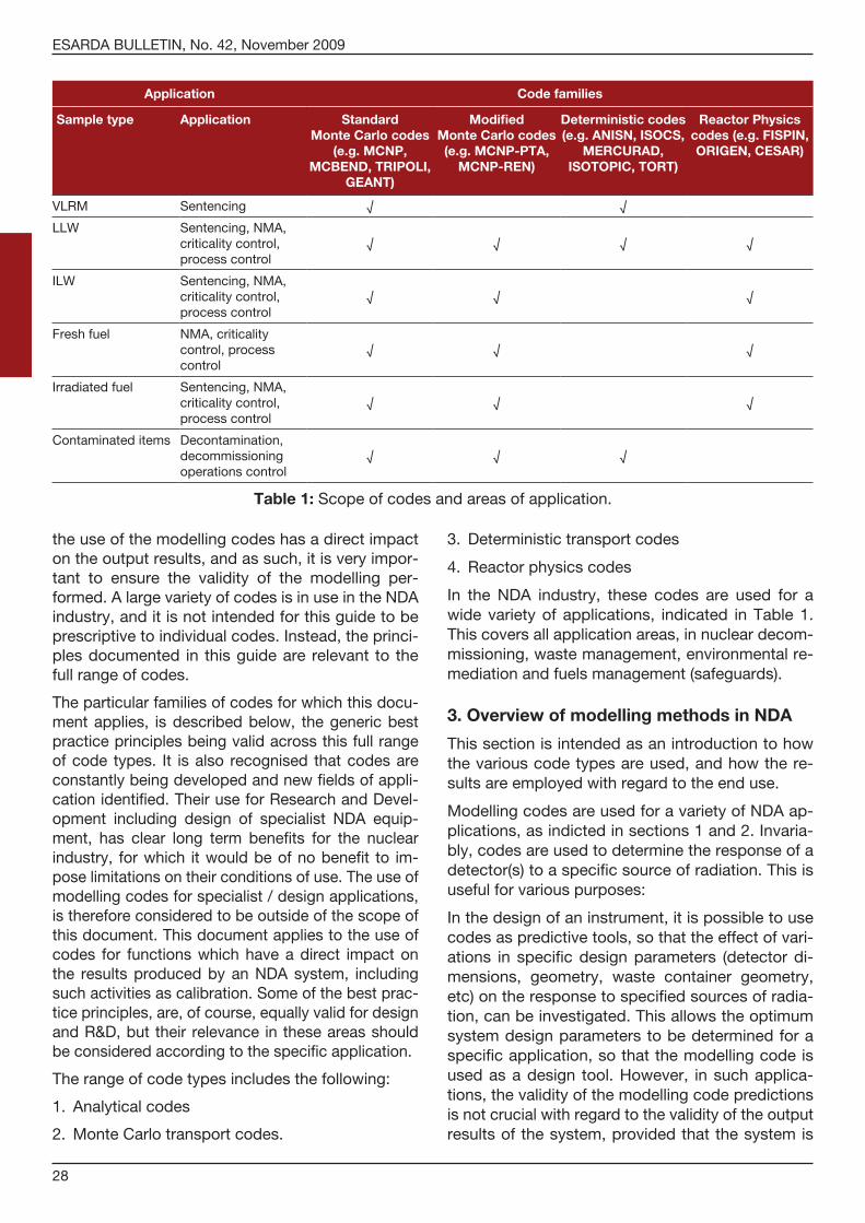
In the NDA industry, these codes are used for a wide variety of applications, indicated in Table 1. This covers all application areas, in nuclear decom-missioning, waste management, environmental re-mediation and fuels management (safeguards).
3. Overview of modelling methods in NDA
This section is intended as an introduction to how the various code types are used, and how the re-sults are employed with regard to the end use.
Modelling codes are used for a variety of NDA ap-plications, as indicted in sections 1 and 2. Invaria-bly, codes are used to determine the response of a detector(s) to a specific source of radiation. This is useful for various purposes:
In the design of an instrument, it is possible to use codes as predictive tools, so that the effect of vari-ations in specific design parameters (detector di-mensions, geometry, waste container geometry, etc) on the response to specified sources of radia-tion, can be investigated. This allows the optimum system design parameters to be determined for a specific application, so that the modelling code is used as a design tool. However, in such applica-tions, the validity of the modelling code predictions is not crucial with regard to the validity of the output results of the system, provided that the system is
Application Code families
Sample type Application Standard Monte Carlo codes
(e.g. MCNP, MCBEND, TRIPOLI,
GEANT)
Modified Monte Carlo codes (e.g. MCNP-PTA,
MCNP-REN)
Deterministic codes (e.g. ANISN, ISOCS,
MERCURAD, ISOTOPIC, TORT)
Reactor Physics codes (e.g. FISPIN, ORIGEN, CESAR)
VLRM Sentencing √ √
LLW Sentencing, NMA, criticality control, process control
√ √ √ √
ILW Sentencing, NMA, criticality control, process control
√ √ √
Fresh fuel NMA, criticality control, process control
√ √ √
Irradiated fuel Sentencing, NMA, criticality control, process control
√ √ √
Contaminateditems Decontamination, decommissioning operations control
√ √ √
Table 1: Scope of codes and areas of application.

ESARDA BULLETIN, No. 42, November 2009
29
calibrated in the traditional manner, using physical radionuclide ( / ) sources or nuclear material (usu-ally plutonium / uranium).
The other main application area for modelling codes, is in the direct calibration of NDA instru-ments. In these applications, codes are used as a direct replacement for physical radionuclide sourc-es and / or nuclear material. This represents a sub-stantial diversion from traditional methods relying on physical reference standards. However, the de-creasing availability of such standards, combined with the increasing accessibility of powerful com-puting technology, increases the arguments in fa-vour of this method. The advantages are obvious, in that physical reference standards are no longer re-quired. However, the disadvantages are obvious, since the confidence that is obtained by calibration with real physical standards that are known to be highly representative of the actual material to be measured by the system, is absent.
There are various NDA applications where model-ling codes are being used increasingly in support of direct system calibrations. It is incumbent upon the organisations that perform such system calibra-tions, to ensure a high degree of confidence in the validity of the predictions from the modelling codes. This confidence comes from a number of technical and non-technical factors, including the following: appropriate definition of the modelling objectives, operator training, Quality Assurance procedures, model validation / benchmarking, appropriate phys-ics techniques and use of nuclear data, and treat-ment of modelling uncertainties.
In summary, the application areas commonly cov-ered, include the following.
• Instrumentdesign.
• Instrument performance modelling (sensitivitystudies etc.).
• Calibration(absolute,relative,andextendingcal-ibration ranges by way of extrapolation or inter-polation for example to extend the calibration based on 252CfmeasurementstoPuitemswithdifferent shape).
• Calculation of correction factors (for exampleself-absorption factors in gamma spectrometry, self-shielding factors in active neutron counting, neutron self-multiplication in passive neutron counting, relative responses for different waste matrices) for which measurement with represent-ative physical standards is impractical.
• Assessmentofshielding/background/interfer-ences such as cosmic-rays.
• Specialistexpertreviewassessments/Interpre-tation of unusual assay results.
• Characterisationofitems(e.g.Burnupcodesforinventory / SNF).
• Uncertainty assessments (by calculating rangeof response for different conditions, such as container wall thickness, waste matrix, source distribution).
• Calculation of spectrum shapes for specificmeasurement scenarios.
• Assessmentofeffectsofdesignchangestoas-say system performance, for example source spectrum tailoring, and effects of changing the detector geometry.
• Calculationofeffectsofsourcespectrumtailor-ing, on instrument performance.
• Shieldingcalculationsforradiationsafetystudies(calculating the dose rate as a function of source – detector geometry and different complex shielding configurations).
Below, we present a number of examples which des-cribe the way that modelling codes have been used to tackle a range of different types of problems.
In addition to these common applications of system calibration and sensitivity studies, NDA system de-signs sometimes employ modelling codes embed-ded within thee core software / analysis engines. For example, some gamma scanning systems such as the Tomographic Gamma Scanner [3] employ ray tracing codes for assessment of waste contain-er matrix attenuation properties.
ThemostwidelyusedMonte-CarlocodeinthefieldofnuclearmaterialmeasurementisMCNP[4].
Other widely used Monte Carlo codes includeMCBEND[8]andTRIPOLI[9]andtheGEANTsys-temusedatCERN[10].
3.1. Example 1: Calibration of neutron counters using Monte Carlo
One of the main applications of numerical simula-tion of NDA techniques is the calibration of neutron counters.
The main complication in the calibration procedure of NDA techniques derives from the extremely high sensitivity of these measurements to a lot of param-eters: geometry (shape and dimension), chemical/physical form, container, impurities. An accurate calibration procedure requires a set of standards being as similar as possible to the samples to be measured. This means that a large variety of refer-
ESARDA BULLETIN, No. 42, November 2009
30
ence materials have to be produced to represent all the possible items of the nuclear fuel cycle subject to accountancy verification. The geometry of the sample, for instance, has a big importance on the response of neutron counters. Generally different calibration curves have to be established for each typeofcontainer.Presenceofothermaterialsinthesample matrix and/or in the container walls affects as well NDA measurements. Heavy materials shield gamma rays, whether light materials moderate neu-trons changing dramatically their behaviour. Even the presence of determined elements (like boron, beryllium, and cadmium) as impurities at trace level can perturb the result. Uranium enrichment and plu-tonium isotopic composition introduce a further pa-rameter influencing the measurement and contrib-uting to the proliferation of standard requirements.
Due to the high number of (sometime costly) special fissile reference materials required by NDA tech-niques, it becomes fundamental to investigate and develop methodologies giving the possibility to re-duce these requirements. Here is where computa-tionalmethods,andinparticularMonteCarlosimu-lations, can play an important role. Having a suitable model for instrument simulation, it is no longer strict-ly necessary to have a reference material identical to the sample for instrument calibration. A single well-characterised standard can be used as a representa-tive of a wide class of “similar” items and to establish a “basic” calibration. Then it is possible to compute withtheMonteCarlothedeviationfromtheidealbe-haviour (represented by the basic calibration curve) due to the presence of relatively small differences between the real sample and the standard: geome-try, presence of other elements, different chemical/physical properties, effect of isotopic composition, etc. Another possibility is to use calculations to ex-trapolate an experimental calibration curve beyond the boundaries fixed by the available standards.
We call this first lower level “soft” application of calculation to the calibration process. The calibra-tion procedure is still strongly relying on experimen-taldata.Calculationsinterveneonlyata“relative” level producing just corrections to the experimental calibration. Since the correction factors are gener-ally second order terms of the basic response func-tion, the accuracy requirements for the calculations are not so demanding. For instance when the effect of the simulated deviation from the experiment is lower than 10% of the global instrument response, an accuracy of a few percents in the relative correc-tion factor is certainly enough.
Nevertheless there could be situations where cali-bration standards identical, or even similar, to the
item are not available. In this case the experimental calibration is impossible and we need to establish a calibration procedure entirely based on computa-tional modelling. We call this extreme case “hard” application of calculation. Of course, no matter how much we can trust our confidence in our modelling capabilities, a totally blind application of a compu-tational calibration would be extremely dangerous. BeforeanyuseofMonteCarlofor“absolute” cali-bration, the model has to be extensively validated. A wide series of experimental measures have to be simulated in order to confirm the quality and to as-sess the accuracy of the computational model.
An intermediate case between the “soft” and “hard” extremes happens when a single standard is avail-able allowing the measure of a single experimental point. In this case the full calibration curve has to be produced by calculations and the experimental point provides the validation. In alternative the com-puted curve could be adjusted or re-scaled to fit the experimental point.
Of course the accuracy required for an absolute calibration is much higher than in case of relative applications. The performances of the computa-tional tool should be as close as possible to the re-sults expected from an experimental procedure, that means of the order of 1% or better. This is to-dayat the limitofMonteCarlocapability,butweexpect to improve this situation in a near future, mainly through a reduction of uncertainties on nu-clear data. An extensive use of “hard” computation-al calibration could be soon a reality and a standard widely accepted procedure.
Modelling is used to reduce reliance upon repre-sentative calibration standards, reduce calibration resource needs (manpower) and reduce overall costs. Recent developments and successful bench-marking have shown that such “hard” calibrations can be used, under some conditions, with confi-dence, thus removing the need for absolute refer-ence standards (such as fissile material). A common practice in modelling neutron counting systems is to use calibrated neutron sources (that is, with knownneutronemissionandpurity) insteadofPustandards. For example, 252CfspontaneousfissionsourceshaveaspectrumveryclosetothatofPuand can be used as “transfer” reference standards. They can be used to conveniently represent dis-persedPu (the small physicalmass gives rise tonegligible self-multiplication and self-shielding ef-fects). Modelling is therefore often performed to simulate experiments with a 252Cfsource,forbench-marking and sensitivity studies.

ESARDA BULLETIN, No. 42, November 2009
31
Monte Carlo modelling is most widely used formodelling of neutron assay systems – the estab-lished code MCNP [4] being perhaps the mostwidely used.
3.2. Example 2: Typical approach for in-situ gamma spectroscopy modelling
Modelling codes are often used to perform efficien-cy calibrations in support of quantitative gamma ray spectroscopy measurements, for example in de-commissioning and waste management. Examples include measurements on plant items with geo-metries for which it is prohibitively difficult to con-struct a calibration geometry with the appropriate distribution of sources, such as heterogeneously filled waste drums, and bulk waste items from de-commissioning operations.
It is possible, using commonly available codes, to use computer modelling techniques to calculate the efficiencies for such geometries, thereby permitting quantitative analysis. Modelling tools allow various geometries to be modelled including different shapes of item, container fill – matrix, and source distribution, together with options for the detector details and shielding / collimation.
By modelling the range of such parameters, it is possible to study in a systematic manner, the ef-fects of varying key geometry parameters, on the measurement results, in order to estimate the meas-urement uncertainty. Such studies are not generally practical by measurement, due to the difficulties as-sociated with arranging appropriate sample / source geometries.
Varioustechniquesareusedtoperformsuchcalcu-lations, includingMonte–Carlomodelling (codessuchasMCNP[4]andMCBEND[8]andTRIPOLI[9]) for the detector response function, and “line of sight”attenuationmodels(codessuchasISOCS[5,6and7]andMERCURAD[11and12])todeterminethe sample attenuation and sometimes the detector responsefunction(the“MERCUREv6”softwareisdistributedbyCanberrathroughthe“MERCURAD”human graphical interface). As for neutron applica-tions, it is crucial to ensure that particular measure-ment applications are performed within the defined dynamic range of for which the modelling has been benchmarked and for which code validations, exist. References [5and21]provideexamplesof theseactivities.
With recent advances in modelling methodologies, it is becoming common to model full pulse height spectra (to predict performance under realistic field
conditions), as well as calculating full energy peak efficiencies and relative efficiencies.
3.3. Example 3: Typical approach for reactor physics codes
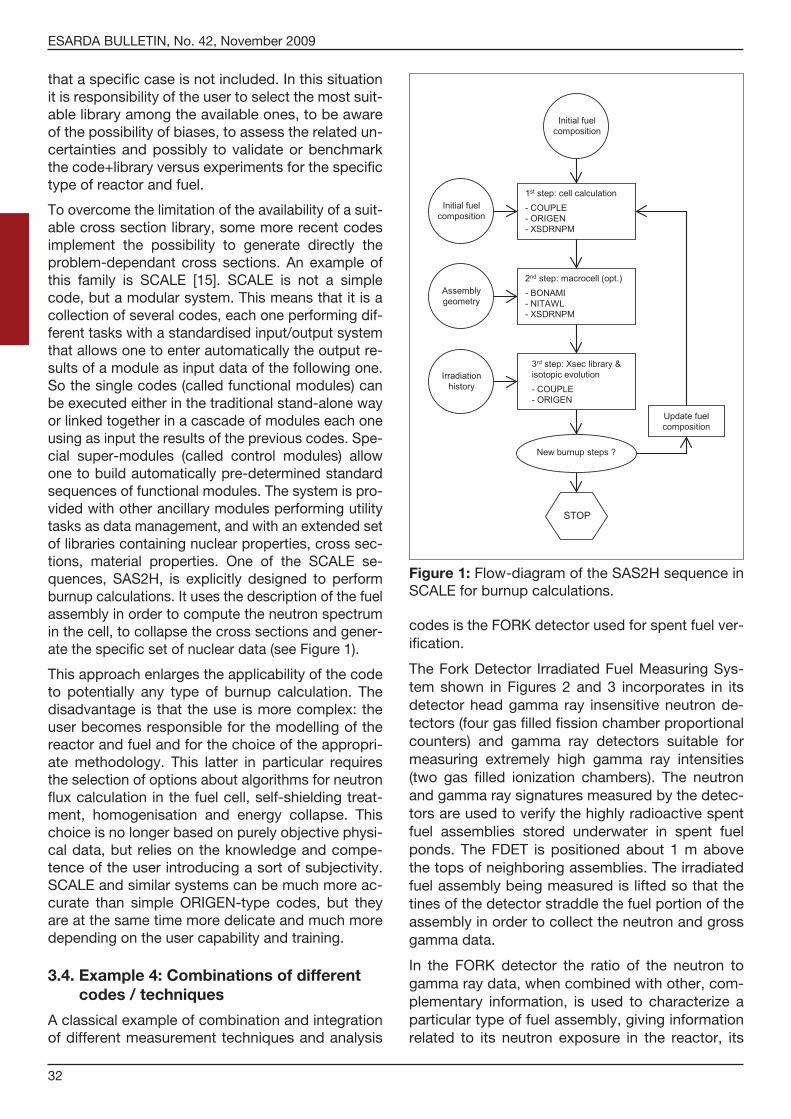
Reactor physics codes in support of NDA measure-ments are mostly used to compute the composition of irradiated materials. In fact, it is often very diffi-cult (or mostly impossible) to measure the mass of nuclear material in irradiated fuel. This is due to the fact that differently from fresh nuclear material where the spontaneous fission neutrons are gener-ated basically from plutonium and can be used for quantitative assay of plutonium mass, in spent fuel the dominating neutron signal comes from (even very small amounts of) curium and overwhelms the plutonium signal. Therefore, being the direct meas-urement of SNM impossible, most of NDA tech-niques aim to the confirmation of the fuel burnup through themeasurement of Cm-generated neu-trons or of fission product photons and the amount of SNM is therefore inferred through the calculation of spent fuel composition using isotopic generation/depletion codes.
The historically most used among this family of codes is ORIGEN [14]. It solves the huge system of differential equations describing the time evolution of any number of isotopes accounting for all types of nuclear decay chains and neutron induced reac-tions. The use of this code is relatively straightfor-ward and accessible for users who are not special-ist in nuclear physics. In fact most of the required input is "objective": that means it requires mostly physical data as initial composition and irradiation history (time and flux or specific power). The major limitation of ORIGEN derives from the availability of nuclear data. In fact, in order to solve the evolution equation accounting for neutron induced nuclear reaction, the code needs to know the 1-group neu-tron cross sections for all isotopes. To obtain an accurate 1-group cross section set, it is necessary to collapse energy-dependant or multi-group cross sections to 1-group by weighing on the energy spectrum of the neutron flux. This step is very deli-cate and requires the use of sophisticated models and codes and a deep knowledge in nuclear phys-ics. For this reason the normal approach is to have libraries developed by specialists who can produce dedicated cross sections sets for any type of reac-tor and fuel. Normally ORIGEN (or similar codes) is distributed together with a wide set of cross section libraries covering the most typical cases and match-ing the most frequent needs. Nevertheless no library set can be fully comprehensive and it may happen
ESARDA BULLETIN, No. 42, November 2009
32
that a specific case is not included. In this situation it is responsibility of the user to select the most suit-able library among the available ones, to be aware of the possibility of biases, to assess the related un-certainties and possibly to validate or benchmark thecode+libraryversusexperimentsforthespecifictype of reactor and fuel.
To overcome the limitation of the availability of a suit-able cross section library, some more recent codes implement the possibility to generate directly the problem-dependant cross sections. An example of this family is SCALE [15]. SCALE is not a simplecode, but a modular system. This means that it is a collection of several codes, each one performing dif-ferent tasks with a standardised input/output system that allows one to enter automatically the output re-sults of a module as input data of the following one. So the single codes (called functional modules) can be executed either in the traditional stand-alone way or linked together in a cascade of modules each one using as input the results of the previous codes. Spe-cial super-modules (called control modules) allow one to build automatically pre-determined standard sequences of functional modules. The system is pro-vided with other ancillary modules performing utility tasks as data management, and with an extended set of libraries containing nuclear properties, cross sec-tions, material properties. One of the SCALE se-quences, SAS2H, is explicitly designed to perform burnup calculations. It uses the description of the fuel assembly in order to compute the neutron spectrum in the cell, to collapse the cross sections and gener-ate the specific set of nuclear data (see Figure 1).
This approach enlarges the applicability of the code to potentially any type of burnup calculation. The disadvantage is that the use is more complex: the user becomes responsible for the modelling of the reactor and fuel and for the choice of the appropri-ate methodology. This latter in particular requires the selection of options about algorithms for neutron flux calculation in the fuel cell, self-shielding treat-ment, homogenisation and energy collapse. This choice is no longer based on purely objective physi-cal data, but relies on the knowledge and compe-tence of the user introducing a sort of subjectivity. SCALEandsimilarsystemscanbemuchmoreac-curate than simple ORIGEN-type codes, but they are at the same time more delicate and much more depending on the user capability and training.
3.4. Example 4: Combinations of different codes / techniques
A classical example of combination and integration of different measurement techniques and analysis
codes is the FORK detector used for spent fuel ver-ification.
The Fork Detector Irradiated Fuel Measuring Sys-tem shown in Figures 2 and 3 incorporates in its detector head gamma ray insensitive neutron de-tectors (four gas filled fission chamber proportional counters) and gamma ray detectors suitable for measuring extremely high gamma ray intensities (two gas filled ionization chambers). The neutron and gamma ray signatures measured by the detec-tors are used to verify the highly radioactive spent fuel assemblies stored underwater in spent fuel ponds. The FDET is positioned about 1 m above the tops of neighboring assemblies. The irradiated fuel assembly being measured is lifted so that the tines of the detector straddle the fuel portion of the assembly in order to collect the neutron and gross gamma data.
In the FORK detector the ratio of the neutron to gamma ray data, when combined with other, com-plementary information, is used to characterize a particular type of fuel assembly, giving information related to its neutron exposure in the reactor, its
Figure 1: Flow-diagram of the SAS2H sequence in SCALEforburnupcalculations.

ESARDA BULLETIN, No. 42, November 2009
33
initial fissile fuel content and its irradiation history (e.g. the number of cycles for which the assembly was in the reactor). The gamma radiation is domi-nated by the fission products, mostly 137Csinagedspentfuel.TheneutronsignalisdeterminedtheCmand Pu isotopes, but in large majority is due to244Cm.Theconfirmationofoperator’sdeclarationofthe initial composition, fuel burnup and cooling time is done by comparing the neutron and gamma ra-diation measured by the detector with the expected composition of the spent fuel computed with inven-tory codes, such as those described in example 3. In parallel the detector calibration (that is conver-sion of 244Cmmass inneutroncount rate)canbedonewithMonteCarlocodesasdescribedinex-ample 1.
TheSMOPYsystem[17]isanothersystemusedforfuel verification measurements. This system uses a combination of neutron and gamma detection to measure the burnup. The methodology combines
measurement of the total neutron emission rate, with the fission product yields and modelling using theCESARcode[18],forburnupmeasurementap-plications such burnup credit assessment.
Combinationsofcodesareoftenused forvariouscombined reactor physics applications, for example theCRISTALcodesystem[19]whichusesacombi-nationoftheAPOLLO,TRIPOLIandMORETcodes.
For decommissioning applications, combinations of measurement techniques / modelling codes are sometimes combined to develop an integrated measurement solution. An example is the combined use of dose-rate simulation with modelling to deter-mine the response function of a detector for a par-ticular geometry. Gamma imaging can support such studies, in order to determine, for example, the lo-cations within a plant glovebox containing the high-est concentrations of holdup. Dose-rate modelling can determine the operator doserate at particular locations, whilst calculations of the detection re-sponsefunction(withacodesuchasISOCS)canallow the activity of measured nuclides, to be quan-tified. Such modelling allows can allow, for exam-ple, glovebox dismantling operations top be opti-mized, reducing operator doserates whilst providing activity assessments for plant items. Examples of such approaches are given in [12 and 13].
4. Best Practice Methodologies
4.1. Problem Definition
Before a modelling campaign can proceed, it is vital that a clear understanding is formulated, of the ob-jectives of the work. The nature of the objectives can heavily influence the modelling techniques de-ployed.
It is recommended that the objectives are clearly documented, to enable the modelling campaign to beconductedproperly.Commonobjectivesincludethe following:
1. Determination of optimum geometry for a par-ticular NDA system design, by making incremen-tal changes in the model to key system parame-ters (it would probably be extremely impractical to make these adjustments experimentally).
2. Investigation of the variability in response of a system, to well defined variations in sample – specific parameters (for example fissile material mass / nuclide activity, waste container dimen-sions, waste matrix composition, etc.).
Figure 2: Drawing of the FORK detector during safeguards inspection measurements. In red: the FORK detector, in green: the fuel assembly to be measured.
Figure 3: Fork detector during safeguards inspec-tion measurement [16].

ESARDA BULLETIN, No. 42, November 2009
34
3. Direct calibration of an NDA instrument, to deter-mine the relationship between the source activity (or mass) and the measurement response.
4. To determine a set of sample – specific parame-ters that are related in some way, to the results of an NDA measurement.
These objectives may each require different tech-niques to be applied, in the use of the appropriate modelling codes.
When used for design of NDA instruments, the re-sults of the modelling are only applied in allowing the system design to be optimised, in a systematic manner that would not have been otherwise possi-ble. It is only the instrument design itself, that has been influenced by the modelling. For these design applications, there are less stringent requirements on the modelling practitioner, than would be the case for direct calibration applications, for example. The designer must have a certain level of confi-dence in the results of the modelling, in order to avoid expensive mistakes in the system design. However, use of the modelling in this way does not have a direct impact on the output results of the NDA system. For such design applications, design-ers often use elaborate features of the applicable codes (e.g. variance reduction techniques) to opti-mise the design process.
Codescanbeusedinapredictivemannertopre-dict the variability in response of a system to identi-fied changes in specific sample parameters. In such case, the codes are used to illustrate the variability in response or output quantity (e.g. mass or activi-ty), but only for illustrative purposes. The results of this modelling may influence the schedule for a measurement campaign later, but they do not di-rectly affect the output result of the system itself. Modelling may be deployed in such a manner, in order to design a measurement campaign, for pur-poses of recalibrating an NDA system, for example. However, the subsequent calibration campaign would then invariably be subject to its own proce-dures. In these applications, it is obviously impor-tant that experience has previously been built up in the use of the code for the particular application. The consequences of not adopting best practice, could be delays to measurement campaigns, per-haps requiring additional radionuclide sources to be procured, with the obvious associated “knock-on” costs.
It is when modelling is used for direct calibration of NDA systems, that the modelling results have the highest importance. In these cases, the modelling has a direct effect on the output of the NDA system.
The consequences of not adopting best practice methodologies, are obviously potentially the most serious, in these cases. One is relying on the mod-elling to determine the relationship between the source-specific parameter (usually activity or fissile mass)and themeasurand.Particularemphasis isplaced on benchmarking, when modelling is used in this way. It is particularly important that the bench-marking has been demonstrated to be applicable across the full dynamic range, wherever possible. In practice this usually means that a particular model-ling technique should be benchmarked to show good agreement between experiment and model, over a measurand range equivalent to that for which a new calibration is being developed. It is also ap-propriate to consider new benchmark campaigns, for example when a code methodology (such as co-incidence counting) is to be applied for a new type of fuel assembly.
Some modelling codes are used indirectly, to relate the output result of an NDA system, to some other quantity. The most common example of this is re-actor physics “burn-up” codes. In these codes, it is common to relate, for example, the 137Cs activity(which is often readily measured by an NDA sys-tem), to the activities of various other un-measura-ble / nuclides and actinides. In such cases, the (otherwise unrelated) result of an NDA system is combined with the results of the modelling code, to yield nuclide activities, which may later be used for waste sentencing purposes. A similar level of strin-gency is therefore required, as for calibration appli-cations, and benchmarking should be considered as equally important.
In documenting the problem definition, considera-tion should be given to the existence of relevant benchmarks, and whether any further preparatory benchmark work is required before a specific mod-elling campaign can proceed.
The following aspects should be considered, as a minimum, when documenting the requirements of a specific modelling campaign:
• What is the end-use project / who is the cus-tomer?
• IsthemodellingrelatedtoanexistingNDAsys-tem (in which case, is there an existing model), or a new system?
• Whatistherangeofsample–specificpropertiesto be considered?
• Whatquantityistobecalculated?
• Howaretheresultstobeused?
ESARDA BULLETIN, No. 42, November 2009
35
• What accuracy is required for the calculated results?
• What precision is required for the calculated results?
• Howarethemodelledquantitiestobeconvertedinto NDA system output quantities (e.g. combi-nationofMCNPcalculatedquantitiestoproducethe neutron counter “Reals” coincidence count rate)?
• Howaretheresultstobereported?
• Whatbenchmarksexist?
• Arenewbenchmarksrequired?
These considerations can determine the modelling techniques to be used. For example, it is possible that documented benchmarks relevant for the spe-cific application, show that it is not possible to achieve the required accuracy, and further bench-marking must be sought. The required statistical precision has a large impact on the length of time to be assigned to the models.
If the results are to be used to calibrate a safety – critical NDA system, there may be specific plant re-quirements that dictate a higher level of stringency with regard to calibration validation.
4.2. Benchmarking / Validation
One of the most important factors regarding the correct use of modelling in support of NDA system calibration / performance testing, is to ensure that the system model is appropriately benchmarked against experiment. In practice, this means that a benchmark measurement is performed, under typi-cal conditions for the NDA system, and a model is performed under identical conditions. Comparingthe measured and calculated system response, al-lows an assessment of the level of agreement, to be performed. The problem definition phase of a mod-elling campaign should define the level of bench-mark agreement, that is required for a specific ap-plication. Modelling results can be renormalized, to take into account any such bias.
Benchmark experiments are used to compare the modelled / measured response for a wide range of geometries, designed to simulate various applica-tions. It is crucial to ensure that particular measure-ment applications are performed within this defined dynamic range, for which established benchmarks andcodevalidations,exist.Reference [5]givesaset of example benchmarks for the widely used ISOCSsystem,whilereferences[20]and[21]pro-
vide example benchmarks for the commonly used MCNPcode.
It is vital that the validity of the model is confirmed throughout the dynamic range of the parameter space to which the model will be implemented. For example, if modelling is being used to determine theeffectofadrummatrixonaPNCCsystemre-sponse, then one should devise a benchmark ex-periment using a matrix which leads to a system response representative of the range of real matri-ces. This means that a benchmark is required which represents the typical range of measurement condi-tions. In practice, if the modelling and measurement results show a discrepancy of say 10 %, this can be interpreted as a fixed bias, and it is therefore ap-propriate to apply this factor as a normalisation constant to all results predicted by the model, if the results are to be used to calibrate an NDA system. In the above example, if the real range of matrices produces a modest variability in response, to say ± 20 %, then a single benchmark with a typical ma-trix within this range, would suffice. However, it would not be sufficient to assume that the same benchmark test is still valid, if a model is to be ap-plied to the same system with a grossly different geometry, for which the response has changed substantially (e.g. changing to cadmium liner mode in active neutron NDA systems).
If a model has been obtained from a contractor or other external organisation, then an appropriate benchmark should be sought, prior to use of the model. Sometimes, this can take the form of ap-pealing to a publication in the open scientific litera-ture, or a referenced communication with the con-tractor.
It is recognised that it is not always practical to ob-tain benchmarks that comprehensively cover the full dynamic range for a parameter space of interest. For example, it may not be possible to obtain a benchmark for an enrichment value for a new fuel element type, because it is impossible to perform a benchmark experiment when a physical sample is not available. In such circumstances, a technical as-sessment should be performed, to assess the im-pact of this lack of availability of benchmark experi-ment data. This may include, for example, inspection of the nuclear data, and an intelligent assessment of whether the extrapolation to a new enrichment value (in the case of the example above), is likely to have any significant impact.
AnotherexampleistheuseofMCNPtoextrapolateto new fuel types, and / or extrapolating to higher masses for which benchmarks do not exist. This

ESARDA BULLETIN, No. 42, November 2009
36
approach may be justified, provided that one has a lot of confidence in the physics methodologies and the validity of the nuclear data used. For example, special physics studies can be performed, to vali-date such extrapolations.
Publishedbenchmarksexistforwidelyusedcodes.ForexampleforMCNP,alargenumberofbench-marks exist for neutron and photon applications [see references 20 and 21 respectively]. For specific NDA application areas such as nuclear fuel verifica-tionbyPNCCassay, specialbenchmarkprojectsare typically organised [see references 22, 23 and 24]. Similarly, benchmarks exist for the gamma-ray attenuationmodellingcodeISOCSandothers[seereferences25and26]. ISOCS iswidelydeployedfor calculating the efficiency of detectors for difficult geometries for which it is impractical to construct representative physical calibration standards.
4.2.1. Case- Study 1: Calibration of neutron counters at JRC
JRC has performed calibrations for DG-TREN(Euratom Inspections) and for the IAEA to provide calibrations of various neutron coincidence count-ing systems for different applications where suitable reference materials for experimental calibration were not available. The description of the different problems, of the proposed solutions and of the ob-tained performances and results are documented in references[27,28,29,30,31,32and33]andcoverseveral applications:
• measurementofHEUfuelswithextremelyhigh235U linear masses
• extension of calibration curves of collars for LWR fresh fuel assemblies with higher 235U enrichment
• calculations of correction factors for burnablepoison in various conditions
• calibrationcurvesforVVERfuelassemblies
• useofAWCCforspecialHEUrods
• passivecollarsformagazinesofMOXfuelrods
• passiveneutronscannerfor“chaussettes”withseveralboxesofPuO2 powders.
We want to summarise here the basic concepts that were applied and the operational procedure fol-lowed in all these cases. This procedure could be used as an indication of good practice for this kind ofapplication.ThebasicprocedureappliedatJRCis based on the following steps:
• measurementinthePERLAlaboratoryofalargeset of reference standards with the same detec-
tor (and eventually the same source for active systems) to be used
• comparisonbetweenMonteCarlo calculationsand the experimental results in order to validate the computational model of the detector
• generationwithMonteCarlocalculationsoftheresponse function of the detector with the spe-cial type of samples
• on-siteverificationofrealsamples.
The development of an accurate model for the neu-tron detector is the most important and delicate task of the entire procedure. The first two steps aim to the validation of the computational model of the detector. Once a fully validated model of a counter has been properly benchmarked, this opens theo-retically the path to the calibration for any kind of sample. Indeed the first two steps validate at the same time the model of the detector and the mod-els of the reference samples measured in the labo-ratory campaign.
It remains questionable how much is reliable the developmentoftheMonteCarlomodelofthespe-cial samples for which the calibration has to be computed in the third step. This is much harder to be proven and it is possibly the weakest point of the suggested procedure, since there is no a-priori way to guarantee the quality of a new model. Of course the situation will be much better when the reference materials used in the first steps are very similar to the special samples: in particular when they have the same geometry, since the geometry is themost delicate parameter of aMonte Carlomodel, where it is higher the probability of making errors. For instance, in the case of the extension of the calibration curve of fresh fuel at higher enrich-ment,thegeometricalmodelofthePWRandBWRfuel assemblies had been validated in the first phase with respect to real measurements, so the extrapo-lation to higher enrichment (involving only the mod-ification of the material composition) was straight-forward and error-proof.
Recommendations from user experience:
Trying to generalise the outcome of the experience coming from the analysis of a large set of compari-sons between calculations versus experiments with neutron coincidence counters, we can draw some general remarks:
• theaccuratedescriptionofthegeometry(dimen-sions, compositions, density) of the detector is of paramount importance

ESARDA BULLETIN, No. 42, November 2009
37
• do not rely on construction drawings and informa-tion provided by the manufacturer, but get the above mentioned parameters by direct measurement
• agreementisgenerallybetterincadmiumlineddetectors (fast or epithermal neutron spectrum) than in fully thermalised assemblies, this sug-gests some refining could be needed in the cross sections of polyethylene, probably in the S( , ) treatment [4] and in the influence of temperature
• forpassivesystemsoneofthemainsourcesoferror comes from nuclear data – 1% in the spon-taneous fission half-life gives directly an uncer-tainty of 1% on efficiency and therefore on To-tals and 2% on Reals
• weknowthemultiplicitydistributionsonlywithhigh uncertainties
• inactivesystemswehavealsotoaddthelimitedknowledge on the interrogation (Am,Li) source spectrum, especially in the low energy tail.
Practically we can conclude that the accurateknowledge of nuclear data is currently the bottle-neckfortheperformanceofMonteCarlomodellingof neutron counters.
4.2.2. Case- Study 2: Benchmark exercises performed for neutron safeguards assay
In recent years, three benchmark exercises have been organised, to establish the performance of MonteCarlomodellingtechniquesasappliedtothesafeguards assay of fissile material. These followed the gradual development and improvement in avail-ability of modelling hardware, and sophistication of interpretational models. These projects include the following:
• RealsPredictionExercise[22]
This project compared a wide range of Monte Carlomodellingcodesandinterpretationalmod-els, applied to calculate the Reals response for a PWR fuel assembly in an AWCC collar. Theproject highlighted the level of agreement that could be achieved using the modelling tools available at the time, and demonstrated the im-portance of nuclear data in producing accurate results. At the time of this project, most of the interpretational models were based on point model approximations.
• SimpleCaseBenchmark[23]
This project was based on a simple neutron slab counting geometry and compared the use of dif-
ferentMonteCarlocodes tocalculate theeffi-ciencyforacalibrated,traceable252Cfradionu-clide reference source. The results were comparedwiththemeasuredefficiency.A252Cfsource was used because such a source is often used to measure and calculate the efficiency for benchmarksystems,toallowMonteCarlomod-elling to calculate calibration parameters in a “relative” sense. The analysis focussed on the effects of different codes, physics treatments and nuclear data. The importance of the nuclear data was shown, in the context of the fundamen-tal limitation that these impose on the accuracy with which modelling tools can calculate abso-lute responses. Areas for further development were recommended, for example in the evalua-tion of a consensus source spectrum term.
• MultiplicityBenchmark[24]
With the increasing availability of powerful com-puting platforms, it is now possible to simulate directly,throughMonteCarlomodelling,there-sponse of neutron coincidence and multiplicity analysis electronics, rather than relying on the in-termediate stage of the interpretational point model which necessitates inherent approxima-tions. This benchmark project is directed at the establishment of a standard modelling code and methodology, which is capable of direct simula-tion of all of the aspects of neutron coincidence / multiplicity analysis systems (efficiency, dead-time, multiplicity distributions and moments, etc.).
4.2.3. Case- study 3: Validations for gamma spectrometry waste measurements [5 and 13]
For in-situ gamma spectroscopy modelling codes a large number of published benchmarks exist (see, for example, references [5 and 13]). However, inview of the versatility of the modelling codes, it is important to be aware of the magnitude of the un-certainties, and the effects of the approximations and assumptions that are made when modelling both the geometry of the physical item to be meas-ured and the spatial distribution of the activity with-in it. For this reason, it is important that the valida-tion carefully bounds the specific assay problem. This is particularly important when seeking regula-tory acceptance of proposed methodologies.
Typically, in the fields of decommissioning and waste management, validation exercises for gamma and neutron assay applications are performed on a project-specific basis, recognising the unique na-

ESARDA BULLETIN, No. 42, November 2009
38
tureofmanyprojectsandwastestreams.Validationoften includes the construction of inactive simulated waste containers with re-entrant tubes inserted, al-lowing placement of radioisotope standards at well defined positions covering the full range from best toworstcasemeasurementscenarios.Comparisonof measurement and calculation then allows a vali-dation to be made for the modelling process. In this context, the terms “validation” and “benchmark” may be used interchangeably. Other validation methods are sometimes achieved through the use of sampling and laboratory analysis. For example, when measuring bags of (homogeneous) soil by in-situ gamma spectroscopy, it is possible to take small samples from various positions throughout the bag. The specific activity of these samples is then measured by laboratory techniques, and com-pared with the overall specific activity for the bag as measured by the in-situ technique.
4.3. Training / Competency
When modelling a physical problem, the quality of the result is a combination of three main compo-nents:
• theuseofacode implementing accurate math-ematical models adequate to describe the phys-ical reality coupled with efficient algorithms to solve the mathematical equations
• theuseofasetofbestavailablephysical data (such as nuclear cross sections) describing the material properties at the best of the current knowledge
• therepresentationofasystemusinganappro-priate geometry model and physical treatments
• anexperiencedandcompetentuser.
The human factor is probably the most difficult component to be assessed. In fact the typical ac-curacy of a method can be evaluated through an appropriate benchmarking campaign and the influ-ence of uncertainties on nuclear data can be de-rived by a sensitivity analysis. There is no way to evaluate a priori the effect on the result of a poor or experienced use of a code.
The ideal user should:
• be capable to understand all the implicationsand consequences of the choice of any param-eter that the code leave free to be set by the user
• utiliseinanoptimalwayallthepossibleoptionsand approximations offered by the technique
• describethephysicalmodelwiththehighestac-curacy reasonably achievable, using simplifica-tions only when clearly demonstrated to be not influent
• assurethatassumptionsandsimplificationsaf-fecting significantly the result are made only in a conservative way, when this concept is applica-ble (for instance in criticality evaluation and dose estimation).
Any quality assurance systems require that any op-erator performing a task is competent and trained to do it. This applies also to the use of codes and physical models. Any individual using a code should have gone through a complete training process in-cluding:
• havinganappropriateeducationalbackground
• participation to dedicated/specialised trainingcourses
• onthejoblearningwithtutoringfromotherexpe-rienced user(s).
Training itself does not guarantee the correct appli-cation of the acquired generic knowledge to a spe-cific problem. The human factor can be improved only through a complete validation process involv-ingtheentire(code+user)system.Insection4.2we have described how a code can be assessed and validated through a large number of compari-sons between calculations and experimental data. Indeed each user should run himself at least a lim-ited number of benchmark cases in problems that are as close as possible to the problem to be solved in order to prove and validate its own capability to model adequately the problem.
4.4. Quality Assurance
This section is not intended as a prescriptive step-by-step procedure. In practice, modelling codes are too complex to simplify along these lines. In-stead, the procedure gives general guidelines which, if followed by specialist NDA staff, will en-sure a high degree of confidence in the validity of the results produced. In any case, NDA specialist staff will be fully trained (see section 4.3) and com-petent in the details of the modelling process, through a combination of experience, and a work-ing familiarity with the operations manuals prior to engaging in any work.
It is important that practitioners of modelling codes take care to ensure that careful records are kept of their modelling work. This ensures traceability, al-

ESARDA BULLETIN, No. 42, November 2009
39
lowing modelling programs to be recreated by oth-ers, and ensuring repeatability.
It is recommended that dedicated logbooks are used to record the working details associated with model development, and for recording input and output data. These logbooks should also be used to record all relevant data and information associ-ated with a modelling program, as described in this document.
For large modelling campaigns, a model specifica-tion document may be produced, providing a tem-plate for running the models, and recording results. This approach is useful if the modelling is to be per-formed by a team of physicists. The model specifi-cation document should contain information such as the geometry models and source descriptions required, the output data required, the format of the results, and the precision requirements (relevant for stochasticmodellingcodessuchasMCNP).Thisapproach can greatly assist the peer review and auditing processes, for applications where a large amount of data is created.
Typical contents of a modelling specification docu-ment are:
• Reference to benchmark applications, demon-strating the validity of the code, for the parame-ter range of interest.
• Referencetobenchmarkedmodelwhichisavail-able, from which a new model for the present application, can be derived, with minimum ex-trapolation / interpolation.
• MCNPmodelsproducedforsimilarapplicationsin previous work.
• Relevanttechnicalreportsproducedinpreviouswork.
• Detailsofparametervariationsrequired.
• Detailsofoutputtalliesrequired.
• Detailsofrecommendedanalysisprocedure/in-terpretational model to convert from model re-sults to system response.
Typical outputs from a modelling program are:
• Checked and Approved Models (MCNP InputFiles).
• ModelCheckingRecords.
• ModellingResults(MCNPOutputFiles).
• Dataanalysisspreadsheetsetc.
• Analysisresults includingdescriptionof the in-terpretational model used to convert the raw out-
put tally from the mode, into a system response quantity (e.g. count rate).
• Technicalreport.
The data to be included in the logbook should in-clude the following information:
• Each page should be numbered, and labelledwith a project reference.
• Author.
• Date.
• Referencenumbertotheparticularprojectthatthe model relates to.
• Reference to a previous model (from which anew model is developed), if applicable.
• Referencetorelevantsectionofmodellingspec-ification.
• Descriptionandsketchesdescribingthemodelgeometry development, allowing a reviewer to follow the model development.
• Changehistory(differencesbetweenmodelsasthey are developed).
• Modeldescription, includingdetails for thefol-lowing:
- Source term (position, energy spectrum, direc-tionality, etc.).
- Materials used for the various parts (cells) of the geometry.
• Full references should be given to supportingdata used to develop geometry models and physics modeling techniques, including engi-neering drawings, measurements, technical papers, etc.
• Recordsofassumptions/approximationsmadein setting up the models.
• Detailsandjustifications,foralldeparturesfromnormal practice (for example, the use of special variancereductiontechniquesinMCNP).
• Recordoftheversionofthecodebeingused.
• Detailsof,andreferenceto,allnucleardataused(e.g. fixed library supplied with the code).
• Commentsthroughout.
• Records ofmodel filenames (input and outputfiles), and directory path structure.
• Recordsoffilenamesforanalysisprogramsandspreadsheets etc.
• Detailsofcomputerruntimesasappropriate.

ESARDA BULLETIN, No. 42, November 2009
40
• Detailsofoutputresults/tallies,anduncertain-ties.
• Derivationandstatementof“fitnessforpurpose”of modelling technique depending on the end-use and consequences (for example with regard to the effect on the output of a measurement system).
• Recordofpeerreviewofmodels.
• Record of any manual “check” calculations / spread sheets which might be performed in order to add confidence in the validity of the modelling code results (for example it is common practice, when setting up new modelling approaches, to check the validity of the results incrementally, to build up con-fidence in each new stage of the approach).
Model checking:
During the development of a geometry model for an NDA system, full use should be made of any in-built or subsidiary geometry debugging facilities. These may allow detailed views to be displayed, with graphical indications of areas with erroneously de-finedgeometry.ExamplesincludetheMCNP-VISEDprogram, available with the most recent distribu-tionsofMCNP.
Models should be checked and validated (“peer re-viewed”) by a physicist, qualified in the operation of the particular modelling code and procedure. Model checking records sheets may be used as appropri-ate to provide evidence that the checking and vali-dation has been carried out correctly.
Typically, when developing a geometry model for a system which is to be used to perform calibrations, model development should proceed (recording full details of the model development process, in the logbook) until a base model has been developed, for which it can be demonstrated that adequate benchmarking agreement can be obtained, with ex-periment. At this stage, the model should be “fro-zen” for future reference, and subject to peer re-view. Normally, parameters of interest (e.g. waste drum dimensions, source geometry, fuel element enrichment, etc.) are then varied, to perform the modelling campaign (it is not normally required to perform peer review for each of these individual models). When used for calibration applications, system details such as the nuclear data libraries, physics tallies deployed, and detector configura-tion, should not normally be varied at this stage, having frozen the base model. However, when used for sensitivity studies / design studies, it may of course be necessary to make modifications of this
kind, in which case additional peer reviews may be performed, depending on the complexity of each particular application.
Departures from established normal practices:
Departures from normal practices (as prescribed in the code manual) should be fully justified and docu-mented. Operators should be fully conversant with the correct methodologies for using a particular modelling code (for example, through completing anMCNPcourse). It is outside the scopeof thisdocument to prescribe specific methodologies for operation of specific codes. However, operators should comply with the conditions of the code man-ual, which generally reflect a large amount of accu-mulated experience from a range of operators (for example, using beta-testing, and input from user’s forums). All departures from these normal proce-dures should be subject to written justification.
4.5. Nuclear Data
4.5.1 Introduction
The design, evaluation and interpretation of NDA measurements invariably require basic physical data such as decay data and interaction coefficients to be available. The experimental and theoretical lit-erature on the determination of such quantities as: half-life; decay scheme; energy; branching ratio;photoninteractioncoefficients;neutroncross-sec-tions; reaction product yields; charged particlestopping powers etc. is vast, in a constant state of change, and can be confusing. The task of collating and evaluating data to create a self-consistent, or at least a screened, reference set is an activity re-quiring specialist knowledge, experience and tools. It can often be a painstaking undertaking and might best be described as a scientific art.
For the most part, therefore, the selection of physi-cal data is best made from a reputable and recent evaluated source which will be maintained. It should be referenced and remain accessible so that other workers may also make use of it to repeat the cal-culations made with it.
A physical measurement is meaningless unless it is accompanied by a statement of the confidence in the results. Similarly the data one uses should have an uncertainty assessment associated with it. For some classes of data this may be hard to provide. If the experimental data base is sparse, contradictory and or highly convoluted with other physical data or if theoretical models have been used to guide the evaluation it is often quite difficult to evaluate the

ESARDA BULLETIN, No. 42, November 2009
41
uncertainties objectively. Some evaluators may pro-vide semi-subjective commentary. Furthermore the uses of the data may not result in a simple sensitiv-ity analysis. For example in calculating the slowing down behaviour of fast neutrons in a material the scattering cross section and chemical binding treat-ment may be sampled many times in a highly prob-lem dependent way. In such cases it is useful to have several evaluated data sets available, perhaps different revisions or perhaps performed by differ-ent groups, to use as reference values, and to re-peat to calculations to find out what impact a par-ticular choice has. It is also valuable to vary the input data systematically in other ways to determine the sensitivity for the problem at hand.
Accordingly we may think of evaluated data as being a convenient source of reference data. The particular evaluation one chooses should ideally yield results that are acceptable against benchmarks relevant to the problem at hand but it is a mistake to think of a particular evaluation as necessarily the best data. An evaluation provides at best a snap shot which is hopefully reasonably representative of the current state of knowledge. The proof of which data set is better than another depends on detailed comparison against careful experiments and this can be rather difficult to decide. Evaluations of difference prove-nance therefore have great value in allowing the user of the information to gauge the impact on the final results of interest to them, of the choice of data.
If a system has been calibrated in such a way that it makes use of a particular set of physical data then it is important that the interpretation of the meas-urements make use of the exact same data in as much as that matters to the outcome. In other words one should be rigorously consistent.
Similarly one cannot change the data used to inter-pret data arbitrarily as new evaluation become avail-able since, although this may result in a ‘better’ de-cay correction, say, it will also result in a discontinuity with what went before and the important purpose of some measurements is to consistently verify the item is unchanged.
Many computational tools have embedded within them data sets which the user can make use of, and the same is true also of some interpretational codes which have preloaded libraries (e.g. MGA). In these cases the user is freed from the burden of searching and selecting suitable sources of data but retains the responsibility of confirming the data is fit for purpose and does not give rise to inconsistencies in use.
The purpose of this “good practice guide” is to pro-vide guidance to ensure that correct procedures are
followed in the selection of nuclear data sets, as part of performing modelling calculations in NDA. The important point here, is that one should follow a defined set of principles, in order to provide con-fidence in the validity of the nuclear data deployed. In practice this includes issues such as what factors need to be considered when selecting the most ap-propriate nuclear data library, and how these data libraries should be managed.
It is outside of the scope of this document, to pre-scribe recommended values for specific nuclear data parameters. The nuclear data must be considered as part of a closed system when used as part of a mod-elling code, and can only be validated as such. How-ever, it is possible, from the extensive benchmark exercises that have been performed in support of the development of modelling codes in nuclear materials safeguards, to comment on areas where further at-tention is needed., and on exercises which indeed provided useful information on preferred nuclear data sets, in the sense that the best agreement was achieved with benchmark experiments.
Wepresentinreferences[34,35,36,37,38,39,40,41 and 42], examples of recent work in the fields of neutron and gamma NDA techniques.
4.5.2. Nuclear data for Monte Carlo simulation of neutron counters
AllMonteCarlocodesforneutrontransportsimula-tion are provided with cross section libraries. For in-stance MCNP, one of the most frequently usedcodes, is distributed with its own set of libraries and continuously new libraries are produced by different laboratories following the demand and the release of upgraded new evaluated nuclear data files (ENDF, JEFF, JENDL and others). A world-wide activity of validation of these data is permanently ongoing.
It is out of the scope of this guide to discuss and analyse the quality of MCNP libraries. Generallyspeaking, neutron counting requirements are not differentfromanyotherapplicationofMonteCarlocodes and no specific improvements are needed, with maybe just the following exception.
All the modelling codes need an adequate description of the medium properties and in the case of codes used in modelling NDA techniques the nuclear data are the most relevant. Often codes are released with their set of nuclear data. Any validation procedure guarantees the correct performance of the code and associated nuclear data, so it has to be considered a uniqueandcompactsystem.Changingnucleardatawill invalidate the passed validation and require a new benchmark of the code with the modified data.

ESARDA BULLETIN, No. 42, November 2009
42
We will provide here a synoptic of nuclear data used in neutron counting. The nuclear data needed de-pend on the kind of application. For instance they are used by some of the interpretation models ap-plied to process the rough measured data. In this section we will consider the so-called “point model” that is generally implemented in the systems based on the multiplicity counting technique.
4.5.2.1. Models for the interpretation of measured data
The point model is at the basis of the multiplicity counting technique [43 and 44]. It states that it is possible to determine the spontaneous fission rate in a plutonium sample by measuring three experimental quantities (the Singles, Doubles and Triples counting rates) and solving the system of the three equations governing the diffusion and detection of neutrons:
where:
F=spontaneousfissionrateinsample,=neutrondetectionefficiency,M=Totalneutronmultiplication (in practice the model requires that the leakage multiplicationML=MT),=( ,n) to spontaneous fission neutron ratio,
fd, ft=doublesandtriplesgatefraction,sj=j-thmomentsofthespontaneousfission
neutron distribution,ij=j-thmomentsoftheinducedfissionneutron
distribution.
The gate fractions fd, ft represent the proportion of the doubles and triples coincidence signal (respectively) which is observable within the fixed, finite duration co-incidencecountinginterval.Reference[45]givesade-scription of the calculation of these parameters.
The nuclear data appearing in the point model equations above are the first, second and third re-duced factorial moments of the multiplicity distribu-tions. They are defined as:
where r is the reaction identification having value s (spontaneousfission)ori(inducedfission)andPr( ) is the multiplicity distribution (probability that in a fission event secondary neutrons are generated). To compute them it is therefore necessary to know the multiplicity distributions for spontaneous and neutron induced fission. The knowledge of other nuclear data is necessary, even if they do not ap-pear directly into the equations. To relate the spon-taneous fission rate (F) to the 240Puequivalentmasswe need to know the specific spontaneous fission neutron emission rate (neutrons per second gram of Pu),whichisdeterminedbythedecayconstant,thespontaneous fission branching ratio and s1 of 240Pu.Then to compute the total plutonium mass (totalPu)from the 240Pueffectivemass,thesamedatafortheother even numbered plutonium isotopes (238Puand242Pu)areused.Moreovertodeterminethe ratio we need to know the specific ( ,n) neutron yields for all the five plutonium isotopes and for 241Am.
In thenotationusedbyLANLandCanberra,onedefinesthesecondfactorialmomentasv2=<v(v-1)>=sum{v(v-1)P(v)takenoverv=1tov_max}andthethird factorial moment as v3=<v(v-1)(v-2)>=sum{v(v-1)(v-2)P(v)takenoverv=2tov_max}.Workinginterms of these factorial moments and in the equa-tions for S, D and T one would therefore use v1/1=v1/1!,v2/2=v2/2!andv3/6=v3/3!explicitlywherevn/n!iscalledthereduced factorial moment. However, in thealternativenotationusedbyJRC(and expressed in equations 1, 2, 3 and 4 above) one works in terms of reduced factorial moments directly such that sj denotes the j-th reduced facto-rialmoments(thatis,theJRCformalism).Thismayappear confusing at first. However it is simply a matterofconvention; thenucleardataandequa-tions are identical. The outcome is that with the (JRCnotation) vn in equations1, 2, 3 and4 it isnecessarytoreplacethesetermsbyvn/n!tocon-vert to LANL notation. Similarly, it is necessary to replace the termsbyn! vnwhenconverting fromLANLtoJRCformalism.
Expressions for the solution of equations 1, 2 and 3 for the three commonly unknown parameters F, and M, are given in references [44] and [46].
4.5.2.2. Nuclear data for neutron transport
InMonteCarlo simulation the entire instrumentaldevice is described and all the possible physical events from neutron generation, during transport, until detection must be adequately modelled. This means that the nuclear data set required is omni-comprehensive. Here we give a short list of physical properties involved:

ESARDA BULLETIN, No. 42, November 2009
43
• crosssectionsforallneutronreactionsforallthematerials contained in the samples, sample con-tainersandneutrondetectors;
• spontaneousfissiondata(half-life,branchingra-tio, neutron yield, multiplicity distributions, sec-ondaryneutronspectra)forevenisotopesofPu,238U and 252Cf;
• induced fissiondata (neutron yield,multiplicitydistributions, secondary neutron spectra, de-pendence from incident neutron energy) for all U andPuisotopes;
• ( -n) reaction data (alpha-decay constant, neu-tron yield in different compounds and emitted neutronspectra) forallUandPu isotopesand241Am;
• interrogation source data (neutron yield andspectrum) for AmLi and other sources used in active neutron counting.
Most of the neutron counters have polyethylene as moderator. At thermal energies lattice effects on neutronscatteringarenotnegligible.MCNPcanusea special thermal treatment, S( , ) [4], to model this effect. Unfortunately only a single S( , ) library is available for polyethylene at 300 K. Extensive stud-ies and the already referred benchmarks have shown some systematic deviations especially in strongly moderated systems. There is also experimental evi-dence of the influence of temperature. Some im-provements in Monte Carlo simulation could beprobably expected by a better modelling of the ther-mal treatment and/or by the production of tempera-ture dependent S( , ) libraries for polyethylene.
In appendix A we provide a collection of neutron nuclear data that derive from the experience in benchmarking NDA instruments and measure-ments.
4.5.3. Nuclear data used in gamma spectrometry
The most common application of modelling to gam-ma spectroscopy in nuclear material safeguards applications is the “physical model” used to inter-pret the gamma spectra ofU andPu and derivetheir isotopic composition according to the intrinsic calibration method. This principle finds direct ex-pression in analysis codes such as MGA [47], MGA-U[48]andFRAM[49]andIGA[50].
In practice, the application of Pu andU isotopicsanalysis codes such as MGA, FRAM and IGA is somewhat different in character, than quantitative codessuchasMonteCarlocodesusedtocalculate
detector responses. The codes use nuclear data but this is relative and based on operational experience and may not correspond exactly to book values. Typically only counting statistics are propagated and this is a weakness. In practice, with these codes, is-sues such as the method of fitting peaks, under-standing peak resolution broadening and methods of stripping the spectral continuum, effects of interfer-ence peaks, etc, are very important, emphasising the importance of understanding the problem, on com-mencement of a modelling program.
The nuclear data necessary to perform this type of analysis are those necessary to compute the gam-ma-ray emissions for the uranium and plutonium isotopes, that reduces to the decay half-lives and the branching ratios, the latter being the probability that following a decay a gamma ray with a specific energy is emitted. There are not a lot of recent and accurate data for branching ratios of uranium and plutonium isotopes, the most complete collection dates back to the 70’s [42].
Nevertheless it is important to remark that when gamma spectrometry is used for isotopic composi-tion determination than for quantitative assessment. This means that it is not required a high accuracy on the absolute values of the individual branching ratios, but a good knowledge of the relative intensi-ties between different energies. This feature has a little bit opened the door to a sort of flexible inter-pretation of the branching ratios to be used in the gamma spectrometry codes.
Based on the fact that experimentally measured branching ratios are known only with large uncer-tainties and on the need to have just accurate rela-tive ratios, the branching ratios are often treated not as nuclear data, but as adjustable parameters. This means that often the branching ratio data set has been tuned by the authors in order to reproduce at the best a set of results on experimental data with well-characterised standards. Of course this empiri-cal approach limits the application of the data set of parameter set-up (no longer to be called nuclear data) only to cases contained within the “phase space” of the trial set. Any change of the kind of ap-plication to materials or conditions outside the vali-dation boundary will cause a lack of validity of the parameter file and require a new validation or a new parameter set. Of course the adjustment of the branching ratios cannot be left arbitrarily free to the ordinary user. Only the real specialist should be al-lowed to change the branching ratios and to release a parameter file with a well-defined range of validity and a new appropriate validation.

ESARDA BULLETIN, No. 42, November 2009
44
This empirical procedure has been followed histori-cally in most of the applications of gamma spec-trometry to nuclear safeguards and has produced excellent results, so it is considered justified even though for a purist it would seem a little bit “handy craft” and cannot be described as a recommended example of a good practice. From a formal point of view the most correct approach would be as fol-lows. The handycraft probably reflects the fact that the book values need changing. Note also that book values apply across the whole range, but MGA only needs differences in groups:
• tofixthebranchingratiosandtheothernucleardata to the best known available value with their associated uncertainties and store them in a unique configuration file independent from the kindofapplication;
• foreachapplicationdomain,benchmarking(seesection 4.2) the performances of the system (code+nuclear data) to a set of experimentaldata;
• to derive accuracy and eventually (applicationdependent)biasfactors;
• toapply“a-posteriori”correctionfactorstoac-count for systematic deviations of the method.
It should be noted that gamma spectroscopy is also, of course, used for quantitative assay of / isotopes in various applications in waste manage-ment and decommissioning, as well as for uranium and plutonium assay in safeguards and waste sen-tencing. As described above, the validity of any modelling used to calibrate these systems, is de-pendant on the existence of established bench-marks, covering the full “dynamic range” of the modelling deployed. In applications where calibra-tion relies on computer modelling to calculate the attenuationofgammaraysinasample(e.g.ISOCS),data libraries describing the mass attenuation coef-ficient as a function of gamma ray energy, are also used. This data is based upon the photoelectric, Compton scattering, and pair-production cross-sections. The basic principles governing best prac-tice of such libraries, are the same as those de-scribed above for neutron cross-sections. The data in these libraries is generally better defined than neutron cross-sections, where there are some known issues for particular isotopes / neutron ener-gies, particularly in regions showing rich resonant structure.
References[34,35,36,37and38]provideusefulfurther reading, on this subject.
4.6. Physics treatments
4.6.1. Physics aspects of cross-section data
To a large extent, and especially as far as neutrons and photons of energy below 20 MeV are con-cerned,thephysicsinvolvedinMonteCarlosimula-tion, is fundamentally based on the nuclear data available to and selected by the user. Taking into account effects such coherent/incoherent scatter-ing, form factors, Doppler and temperature effects, angular distributions, the neutron cross-section data is for instance used to determine:
• Howfarwillaparticletravelbeforecolliding.
• Ifacollisionoccurred,whichcomponentisotopewas that collision with.
• What fraction of the particle weight was ab-sorbed.
• Whichtypeofreactionoccurred.
• Howmanysecondaryneutronsareemittedandfor each of them what is the energy and angle of emission etc.
There are many data libraries available to users and a serious selection of the library to use for a particular application can thus be important for many reasons.
Neutron cross section libraries, for instance, contain in addition to neutron cross section data for tens of reactions, angular and energy distribution for many reactions, heating numbers, reaction Q-values, pho-ton production cross section etc. These libraries have become so simple to use that they are easy to abuse too. They result from processing the nuclear data evaluations and compilations, which them-selves are the fruit of experiments and model codes, usingcodessuchasNJOYtoyielddataeitherinaso called pointwise or multigroup form.
In generating data, various evaluation and process-ing methods are used and many approximations, assumptions and choices are made, such as choice of experiments and representations, interpolation, thresholds, Q-values, representation of angular dis-tributions as equi-probable bins, etc. For the same evaluation, a different processing may also be ap-plied using different processing codes (NJOY,TRANSX, AMPX, SCALE), resulting in either fullcontinuous(classC,e.g.26000.60CinMCNPjar-gon),thinnedcontinuous(e.g.26000.61CinMCNP)or discrete energy data (e.g. 26000.60D), which might also have different temperatures, tolerances etc.Discreteenergyversions(ClassD)ofcontinu-ous energy libraries have often been produced, when computer memory was of essence, whereby

ESARDA BULLETIN, No. 42, November 2009
45
all cross sections are averaged into a fixed set of 262 energy bins.
In choosing neutron cross section tables, one should thus consider the sensitivity of results to dif-ferent evaluations and philosophies, the neutron energy spectra involved, the temperature at which data were processed and the availability of photon-production data. This is achieved by running the modelling codes using cross-section libraries or us-ing special codes designed to produce tailored cross-sections for use by specific modelling codes / applications.
Above20MeVandupto150MeV,somenucleardata has to some extent become available in recent years but this is still insufficient. Thus, a combina-tion of data, nuclear models and various approxi-mations are often made use of to the best one can. Above150MeVtheoreticalmodels,withtheiras-sumptions and approximations are in general the only option.
Electron transport physics is important in some gamma assay modelling applications, where the secondary gamma radiations produced by electron (photoelectrons) interactions, are important for the particular calculation. In electron transport, the physics primarily based also on the cross section data available to which, more approximations (than for neutron transport) are applied and the effects (e.g. bremsstrahlung) considered are more varied. Variousalgorithmsformulti-scatteringareusedinelectron transport which is analogue in essence. The user must be aware of, not all which cross-sec-tion data is used, but also of all the models, algo-rithms and approximations, assumptions and de-faults options (cards) used within a code as to avoid the black box syndrome.
4.6.2. Variance reduction techniques
For problems where analogue simulation is inap-propriate, a non-analogue game can be played by sampling from a distorted transport kernel, whereby the expectation values of the different scores are preserved, whilst the particle histories that contrib-ute most to the required scores are forced to be sampled more frequently. Such methods are uni-versally used for deep penetration problems or highlyscatteringproblems[51,52and53].
The objective of distorting the transport kernel (known as biasing) is to reduce either the variance of the score (variance reduction techniques) or the computer “runtime” (acceleration techniques) need-ed to obtain a given statistical accuracy.
A measure of the success of any biasing method
can be obtained by investigating the ratio
where is the variance on the final score and T is the computer time used to obtain that variance. This ratio is often called the Figure of Merit (FOM) for the simulation. An increase in the FOM, which depends also on the machine used, indicates an in-crease in the efficiency with which the simulation is being performed.
Many effective biasing schemes exist are currently being developed further. Some of the methods, such as particle splitting and Russian roulette, have almost universal application, whilst others, such as the exponential transform, are limited to certain classes of problem. Some of these techniques re-quire care, for example angular biasing may not al-low for scatter build-up properly.
MCNP,forinstance,usesthefollowingfourtypesof variance reduction techniques:
• Truncationmethods:timeandenergycut-off.
• Populationcontrolmethods:weightcut-off,ge-ometry or/and energy splitting and Russian rou-lette, weight window generator.
• Modified sampling methods: implicit capture,general source biasing, forced collisions and ex-ponential transform.
• Partially deterministicmethods: point and ringdetectorsandDXTRAN.
These methods and their application are fully de-scribedintheMCNPmanualandthesampleprob-lempaperforvariancereductioninMCNPbyBooth[54].Ithasbeenshownthatapplyingappropriatelymost of the above techniques to a deep penetration problem example in the Booth paper, one reaches convergence within a few minutes compared to es-timatedyearsofcalculationsona1990’sPC.
Because variance reduction techniques use non-analogue particle transport with no real tracks in-volved, it can happen that portions of the physical phase space may not be allowed to contribute to the results. In such cases, one may not be sampling therightproblembutratheratotallydifferentone;yet giving all seemingly good results that may be inaccurate by as much 2 to 3 standard deviations. This is called false convergence, which is a major pitfall in variance reduction techniques.
This can not happen in analogue transportation (preferred whenever possible) whereby as one is dealing with real physical tracks and particles, one
ESARDA BULLETIN, No. 42, November 2009
46
can not force too much sampling in one area of im-portance or direction, thus ensuring that the prob-lem to be modelled contains all the source particles. Despite ever more powerful computers, variance reductions techniques are often required in many deep penetration or high scattering problems. How-ever and fortunately many NDA applications such as detector response calculation would not require variance reductions and acceleration techniques in general. Furthermore codes such asMCNPhavenow installed statistical packages that if added to user experience and open eyes can avoid help in avoiding such pitfalls.
InaMonteCarlosimulation,theaverageunderlyingbehaviour of the system is inferred from the sam-pled behaviour of simulated particle histories by in-vokingtheCentralLimitTheoremofmathematicalprobability on which the techniques is fundamen-tally based. It is thus only appropriate to mention here that one needs to check that central limit theo-rem is satisfied.
MCNPhasarguablyoneofthemostrobuststatisti-calanalysispackagesofallMonteCarlocodes.Inaddition to the usual mean and variance, the user is providedwith the varianceof the variance (VOV),which involves the first four history score moments and represents the error of the error. The tally score probabilitydensityfunction(PDF)isestimatedandten statistical checks are incorporated to avoid false convergence. False convergence is quantitatively characterised by the non-existence of the variance or mean (1st and 2nd moments) and thus the non-satisfaction of the central limit theorem, which is the most fundamental principle in the Monte Carlomethod. By inspecting the slope of the tail of the underlying tally score PDF one can estimate thenumber of moments that exist and hence determine whethertheVOV,thevarianceandeventhemeanexist. The VOV ismore sensitive to large historyscores and should decrease as 1/N where N is the number of histories.
Sensitivity to other factors such as sample density, container wall details and moisture content, do not produce Gaussian shaped uncertainties. Therefore special consideration (normally through sensitivity studies) is required to determine the shape of their distributions to allow propagation to calculate the correct TMU. The effect of each parameter varia-tion, on the output, must be carefully studied, sam-pling results using a known probability distribution to represent the realistic possible range of the pa-rameter (for example Gaussian, rectangular, or tri-angular distribution). A similar sampling exercise
would then be followed to combine the effects of simultaneous variability in different parameters.
4.6.3. Thermal effects and related issues
Thermal neutron transportation is complicated by the fact that neutrons do not see a single nucleus but the entire molecule and because the velocity distribution (Doppler broadening) of the target at-oms and molecules in the laboratory frame cannot be neglected. Target nuclei are put in motion by the zero-point motion and non-zero temperature of the material as the neutrons tend to be thermalised to the corresponding energies. Low energy and wave-length neutrons may interact with the lattice spac-ing of the solid thus creating peak structures in cross sections, each one corresponding to a par-ticular set of crystal planes. Furthermore coherent scattering (interference of scattered waves) add constructively in some directions and destructively in others thus affecting the angular distributions (Bragg scattering). The double differential cross sections are also modified as neutrons can loose or gain energy in discrete amounts.
Temperature effects are difficult to model and can be particularly important if AE/kT is small where A is the atomic weight of target, E the neutron energy, k the Boltzmann coefficient and T is the temperature. Consequently,inmanyproblemswherethermalisa-tion(<4eV)isinvolved,thethermalS( , ) tables [4] should be invoked to model the neutron scattering as impacted by the binding of the scattering nucle-usinthemoderator.InMCNPthermalS( , ) tables are invoked using the MT card to model the neutron scattering as impacted by the binding of the scat-tering nucleus in the moderator. The isotope scat-tering data is then overridden if one is in the S( , ) energy range.
When comparing the response functions of various polyethylene moderated detectors used in NDA measurements, the agreement obtained is generally better for cadmium lined detectors (fast or epither-mal neutron spectrum) than for fully thermalised as-semblies. This may suggest that one may need to refine our use and knowledge for polyethylene, per-haps as far as the S( , ) treatment and temperature effects are concerned. Agreement is also often bet-ter for cylindrical assay chambers, than for square chambers, indicating the greater degree of difficulty in accurately modelling the multiple scattering of neutrons in corner regions of the latter geometry (where the effects of any inaccuracies in cross-sec-tion data will become more pronounced).

ESARDA BULLETIN, No. 42, November 2009
47
A test example is shown in Table 2 whereby a neu-tron collar detector installed at a processing plan was modelled with and without the S( , ) treatment foramagazinefullofMOX(MixedPu-U)oxidere-actorpins [55]. Thedifference inReals rates, thebest signature for verification, is as much as 7.9%. It is 4.2% for Totals rates.
Collar counter – MCNP modelling method
Calculated quantity
Count rate (s-1)
Ratio of result (with / without thermal treatment)
with S( , ) treatment
Reals 1.1999E+04 7.9%
Total 3.4423E+05 4.2%
without S( , ) Reals 1.3023E+04
Totals 3.5948E+05
Table 2:MCNPcalculatedRealsandTotalscountrates for a Collar (for a MOX fuel pin magazine)counterwithandwithoutthermaltreatment[55].
4.6.4. Neutron multiplicity distributions
In assessing uncertainty budgets and sensitivity analysis, one must bear in mind that a poor knowl-edge or inadequate use of the multiplicity distribu-tions can generate large uncertainties.
Insomecodes,aspreviouslydone inMCNP, thenumber of neutrons generated in a fission event is calculated by sampling only two values:
• Integer(< >)withprobability=1–[< >–Int(< >)]
• [Int(< >)+1]withprobability=[< >–Int(< >)]
While this is reasonably adequate for reproducing, for a large number of events, the average number of neutrons,< >,anditsderivativesrelatedtothefirstmoment such as neutron fluences, coincidence rates which are associated with higher moments of the multiplicity distributions are not correctly mod-elled in sampling the number of fission neutrons. Recent modelling codes have successfully mod-elled the true multiplicity distributions correctly, however.
4.6.5. Importance of random numbers in Monte Carlo modelling
MonteCarlosimulationalsoreliesheavilyonusingrandom (or pseudo-random) number generators. Thus one must ensure that the random number generator used is sound and that any correlations between various calculations that may be due to using the same starting pseudorandom number is removed, as has been shown for example at the
NationalPhysicalLaboratory[56]investigatingtheresponse functions and effective centre of a moder-ated BF3 counter at various energies and distances from the neutron source. In such cases one should ensure that a different random starting number is chosen randomly to avoid unphysical structures and effects in the distributions and entities studied.
References [4,51,52,53,54,55and56]provideuseful further reading, on this subject.
4.7. Treatment of Uncertainties
In this section we define the different kinds of un-certainties, that are relevant for computer modelling applications in the field of NDA. We describe best practice formalisms for expressing the uncertainties of (modelled) quantities, and how to propagate them to give their contributions towards the total measurement uncertainty of the end result of a measurement, consistent with established practice for NDA measurements (see for example [1]). Illus-trations are given with reference to examples of typical modelling applications, including typical sources of uncertainty, and how they are expressed, quantified and propagated. The best practice pro-cedures recommended here are consistent with the industry-recommended guidelines for treatment of uncertainties in NDA measurements, noting that modelling techniques are simply tools used to pro-vide some of the parameters (most commonly the measurement parameter) required to evaluate the result of an NDA measurement (usually fissile mass or nuclide activity).
In the last decade, modelling and simulation have been increasingly used in scientific research and in the analysis and design of engineering systems. Studies have been devoted to the estimation of the total modelling and simulation uncertainty in com-putational predictions (see references [57 and58]and the references herein). These studies generally consider different definitions of uncertainty and error than those defined and used for experimental meas-urements.Commonlyonecandefinethefollowingcomponents: variability, uncertainty and error.
Variability describes the inherent variation associ-ated with the physical system or the environment. It is generally represented as a distributed quantity (e.g. the exact dimension of a manufactured part). Variability is also referred toasstochasticuncer-tainty, aleatory uncertainty, inherent uncertainty and irreducible uncertainty.
Uncertainty describes the source of nondeterminis-tic behaviour and is sometimes also indicated as epistemic uncertainty and reducible uncertainty. Un-

ESARDA BULLETIN, No. 42, November 2009
48
certainty may be defined as a potential deficiency in the modelling or simulation process that is due to lack of complete knowledge (e.g. due to vagueness, nonspecificity or dissonance). As a consequence, uncertainty may be reduced by increasing the knowledge. Uncertainty typically is represented by modern information theories (e.g fuzzy set theory).
Error is defined as a recognizable deficiency in any phase of the modelling and simulation that is not due to lack of knowledge. Examples of errors are the finite precision arithmetic in a computer, ap-proximations made to simplify the modelling of a physical process, mistakes or blunders made by the analyst. Errors may be acknowledged (recognized, magnitude is known) or unacknowledged (not rec-ognized, but recognizable) The term “Bias” is often used to represent the fixed deviation between the true value and the measured value, as a result of such errors or mistakes.
According to these definitions, variability and un-certainty differ from the error by the fact that the first two deal with a level of knowledge that is known (albeit this knowledge may be incomplete), while error deals with knowledge (and therefore a potentialbiasintheresults)thatisunknown.Varia-bility and uncertainty will produce stochastic, non-deterministic effects, whereas errors yield a repro-ducible or deterministic bias in the simulation.
Usually, the term “uncertainty” is used to embrace the above – defined terms “variability” and “uncer-tainty”. At this point, it is important to understand the difference between the commonly used terms “random” and “systematic” uncertainties. A random uncertainty is defined by a distribution of possible values of the parameter, centred about a mean val-ue, usually corresponding to the true value. The na-ture of the distribution function (e.g. gaussian, rec-tangular, triangular) is important. A systematic uncertainty represents as fixed bias or “error”, such that every measurement is different from the true value,bythesamefixedamount.Poissoncountingstatistics is the most common example of a random uncertainty. This terminology has been largely su-perseded by the terms “Type A” and “Type B” un-certainties[59].TypeAuncertaintiesarethosethatcan be evaluated by statistical means, whereas Type B uncertainties must be evaluated by other means.Countingstatisticsisacommonexampleofa Type A uncertainty, whereas the effect of an un-certain waste matrix, is typically represented by a Type B uncertainty because the uncertainty could be manifested as a fixed bias or “offset”.
In the field of NDA measurements / modelling, both types of uncertainty can be important. For example, consider the gamma measurement of drums of waste where drums can be classified according to density. Each nuclide activity measurement will be subject to random counting uncertainties. However, the uncertainty on the final activity may be a func-tion of the drum density. For example, it may be known that a certain waste matrix type / density, always gives the same bias, due to the effect of the physics algorithms being always the same for that type of matrix. In this sense, the observed bias in the end result contains both random and system-atic components. Thus when talking about drums of that particular matrix type, we can talk about a systematic uncertainty of say “10 % underestima-tion”, as well as a purely random component due to counting statistics. However, when considering a random population of drums containing different matrices, the distribution of systematic bias can usually be treated as a random distribution. Similar examples are also applicable for the results of com-puter modelling, applied to NDA applications.
The term “precision” is often used to represent the repeatability of an observation, measurement or calculation. In the absence of any bias or system-atic error, it is often the case that the mean value converges on the true value, if a large number of observations is made. The term precision is often used to represent random, statistical or “Type A” uncertainties.
The term “accuracy” is used to describe the close-ness of an observation (measurement or calcula-tion) to the true value. Thus an accurate measure-ment is one with a low bias and uncertainty.
The term “Total Measurement Uncertainty” express-es the total uncertainty associated with a measure-ment. It includes both the random and systematic components, and requires careful propagation of the individual terms.
Further reading on the expression of uncertainties canbefoundinreferences[59,60,61,62,63,64,65,66,67and68].
This section aims at summarizing the most impor-tant sources of variability, uncertainty and error in computer simulations related to non-destructive as-say and characterization of special nuclear material. This discussion on uncertainty is equally valid for the use of modelling codes for other NDA applica-tions (i.e. for measuring radionuclides that are not, in themselves, classified as special nuclear materi-al). It is assumed that commercially available and validated codes are used for that purpose.

ESARDA BULLETIN, No. 42, November 2009
49
4.7.1. Estimation of total uncertainty determined by the variability of input
Typical simulation problems that are considered here are: particle transport and interactions (neu-trons, photons, electrons…), burnup and depletion computations, criticality calculations. These prob-lemsarestudiedwithMonteCarlocodessuchas:MCNP,KENO,MCBEND,TRIPOLI,MORSE,EGS4,PENELOPE,MONK,ITS,FLUKA,LAHET,ordeter-ministic discrete ordinates codes such as: ANISN, DOORS,DANTSYS,PARTISN,TWOTRAN,CEPXS/ONELD, or simple gamma ray attenuation codes such as ISOTOPIC, ISOCS, MERCURAD / PAS-CALYSandGAMMASHIELD.
Most of the physical parameters describing these problems are identifiable as variability e.g. each pa-rameter may be represented by a distribution. The important point here, is the uncertainty knowledge of what is the true value of a parameter, which leads to an uncertainty in the end result of the simulation. The total uncertainty resulting from the variability of different parameters is obtained by the well known uncertainty propagation laws. If the simulation re-sult is represented as a response F that, given a set of input parameters i and i each with its variability
i, defines the output then the variability on a simu-lation result R can be represented as :
Evaluation of the covariance terms requires that the matrix of behaviours is analysed.
TypicallyadvancedMonteCarlomethodsusethetechnique of differential sampling that computes the derivatives of the response with respect to some of the input parameters at the same time as the re-sponse are used for that purpose. Differential sam-pling with respect to material parameters is availa-bleinMCNP[4].Insuchcomputationsoneormoreof the parameters is varied between its boundaries and the variation of the result is observed. Since not all parameters are independent of one another it may be necessary to investigate possible correla-tions. However, for codes where such differential analysis is not available, it is necessary for the user to quantify the individual uncertainties by a compre-hensive sensitivity study, exploring the sensitivity of the end result to variability in the parameters for which the true physical value is not known.
Interval mathematics is the simplest way to repre-sent total uncertainty when only the bounds of pa-
rameters under concern are available. Each uncer-tain parameter is described by an interval number.
Another approach is to use response surface meth-ods which are used to assess variabilities. The only way to determine the uncertainty will be by using the simulation code itself.
4.7.2. Analysis of different types of uncertainty
Table 3 lists the most important parameters gener-ally used in simulation programs considered in this document.
The physical dimensions:
A problem definition (see section 4.1) for the simula-tion of particle transport requires that the dimensions of all objects are properly defined. In practice the di-mensions are only known with limited accuracy e.g. thedeadlayerofaHPGedetectorcrystal,thespe-cificshapeoftheHPGecrystalwhenitisbulletized,the effective length of the anode wire in a ³He detec-tor tube etc. In these situations the best estimates should be used for these parameters, and it may be necessary to investigate the impact by considering different values for these parameters. In many situa-tions the actual geometry is simplified, and details (e.g. small objects) which are believed not to be im-portant arenot considered in the simulation.Careshould also be used in determining where the actual problem ends in space (e.g. it may be necessary to consider reflection by nearby walls that at first sight may appear as not being part of the problem).
Chemicalcomposition:
It is the properties of the materials that build the problem geometry that will determine the transport of particles and their interactions with these materi-als. Depending on the values of the cross sections for certain interactions some elements or isotopes may have an important impact on the result. Hence the material compositions should be considered with care, and laboratory analysis may be required to determine the actual composition of certain ma-terials in the problem. Moreover in some problems, attention should be even paid to trace elements or impurities that may exist in the materials. If these impurities have large interaction probability with the particles considered (e.g. neutron poisons) neglect-ing these may result in strongly biased results.
Material density:
The density of materials together with the composi-tion determines the reaction rates of the particles
ESARDA BULLETIN, No. 42, November 2009
50
that will interact with the material. The density of ma-terials is often looked up in standard tables describ-ing the physical properties of materials, however in practice the actual density may deviate from these values and it may be required to determine the den-sity (e.g. the density of polyethylene used as neutron moderator). For gas filled detectors it is very impor-tant to know precisely the gas pressure and eventu-ally to correct for temperature in order to determine the number of atoms per unit volume. The density and composition of any gamma shields / collimators (especially graduated filters) is obviously important.
Nuclear data:
Cross sections are generally part of the simulationcode and the user may not have to provide these. However in some simulation codes the user may se-lectthecrosssectionlibraries.Crosssectionsshouldbe selected with care and with judgment expertise: the libraries should be fit for purpose e.g. the temperature at which cross sections are given should correspond to the considered temperature in the problem, when considering discrete energy groups, the grouping should be apt for the problem considered.
For gamma calculations, the half-lives and gamma attenuation cross-section libraries are relevant. The branching ratios and abundances of gamma emis-sions are important for quantitative gamma spec-troscopy calculations, while knowledge of the neu-tron yields and multiplicity data is critical to understanding the uncertainties for neutron count-ingmodelling.Calculationsperformedwithdifferentcredible data sets may be used to estimate the state of knowledge uncertainty.
MonteCarlocalculationstatistics:
InMonteCarlosimulation,oneofthemostimpor-tant computational parameters is the number of ini-tial particles that is run. Most codes consider the influence of this parameter and report results to-gether with a relative uncertainty due to the finite number of histories that were run. This uncertainty however may not be considered as the total uncer-tainty. Consideration should also be given to thestatistical convergence of a tally, as the number of source particles increases. Some codes, for exam-pleMCNP[4],providetoolsformonitoringthiscon-vergence. If tallies are “well behaved”, then the standard deviation will be inversely proportional to the square root of the number of source particles that have been tracked. However, it is possible that rare events (for example occasional contribution from very high weight particles) can give large step changes in tallies, causing departure from this nor-
malbehaviour.MostMonteCarlocodesautomati-cally provide statistical uncertainties as part of the normal output, so this component is easy to assess. Tally fluctuation charts should be inspected to check for such behaviour, with reference to the guidelines in the code manual (for example, [4]).
When using physics – based “variance reduction” techniquesto“accelerate”MonteCarloruns,effec-tively increasing the number of source particles that are tracked, great care must be taken to ensure that correct procedures are followed in accordance with the recommendations of the code authors and es-tablished benchmarks, in order to ensure that the results are reliable, and that no significant bias (sys-tematic error or unacknowledged error) is apparent (see section 4.6 for further discussions on this sub-ject). Techniques appropriate for one type of prob-lem (for example uncollided flux) may not be suita-ble for some other types of problems (for example where scatter contribution is needed).
Possiblesourcesoferrororbias:
Sources of error, as defined above, may be identified at two distinct levels: errors induced by the user of the code (e.g. simplifications used to describe the prob-lem with the input parameters) and errors inherent to the code (e.g. made by the developers of the code).
Acknowledged errors:
Acknowledged errors are known by the modeller and the magnitude (bias) may be investigated. Some examples of typical acknowledged errors are given in the Table 4.
Unacknowledged errors:
Unacknowledged errors by definition are not ac-counted for when considering total uncertainty. As such, unacknowledged errors are mistakes, which are best avoided by thorough verification. Examples ofunacknowledgederrorsaregiveninTable5.
4.7.3. Total uncertainty in absolute versus relative simulations
Simulations results generally can be used in two ways: as an absolute simulation result (e.g. abso-lutedetectionefficiencyofaHPGedetector)orinarelative way where the actual result is the ratio of two simulation results. Relative simulation results are typically used to predict a response of a meas-urement situation which is not too much different from another measurement situation (e.g. detector response of a point source compared to a small volume source in gamma ray spectrometry).
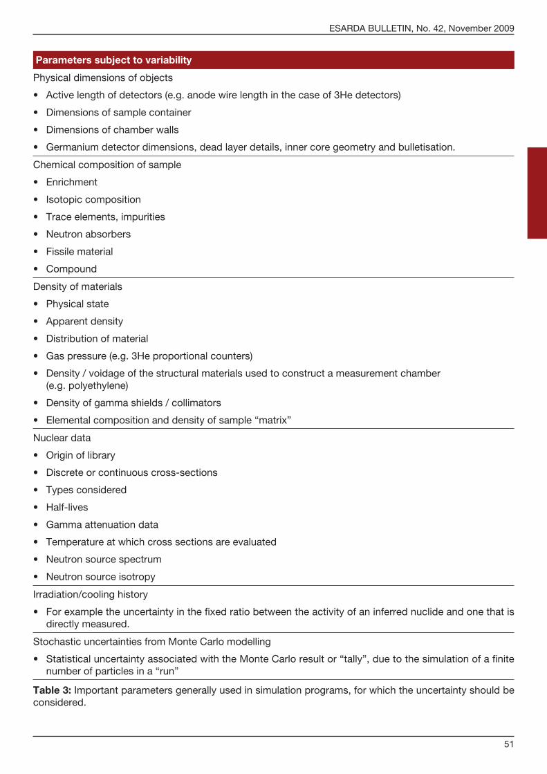
ESARDA BULLETIN, No. 42, November 2009
51
Parameters subject to variability
Physicaldimensionsofobjects
• Activelengthofdetectors(e.g.anodewirelengthinthecaseof3Hedetectors)
• Dimensionsofsamplecontainer
• Dimensionsofchamberwalls
• Germaniumdetectordimensions,deadlayerdetails,innercoregeometryandbulletisation.
Chemicalcompositionofsample
• Enrichment
• Isotopiccomposition
• Traceelements,impurities
• Neutronabsorbers
• Fissilematerial
• Compound
Density of materials
• Physicalstate
• Apparentdensity
• Distributionofmaterial
• Gaspressure(e.g.3Heproportionalcounters)
• Density/voidageofthestructuralmaterialsusedtoconstructameasurementchamber (e.g. polyethylene)
• Densityofgammashields/collimators
• Elementalcompositionanddensityofsample“matrix”
Nuclear data
• Originoflibrary
• Discreteorcontinuouscross-sections
• Typesconsidered
• Half-lives
• Gammaattenuationdata
• Temperatureatwhichcrosssectionsareevaluated
• Neutronsourcespectrum
• Neutronsourceisotropy
Irradiation/cooling history
• Forexampletheuncertaintyinthefixedratiobetweentheactivityofaninferrednuclideandonethatisdirectly measured.
StochasticuncertaintiesfromMonteCarlomodelling
• StatisticaluncertaintyassociatedwiththeMonteCarloresultor“tally”,duetothesimulationofafinitenumber of particles in a “run”
Table 3: Important parameters generally used in simulation programs, for which the uncertainty should be considered.
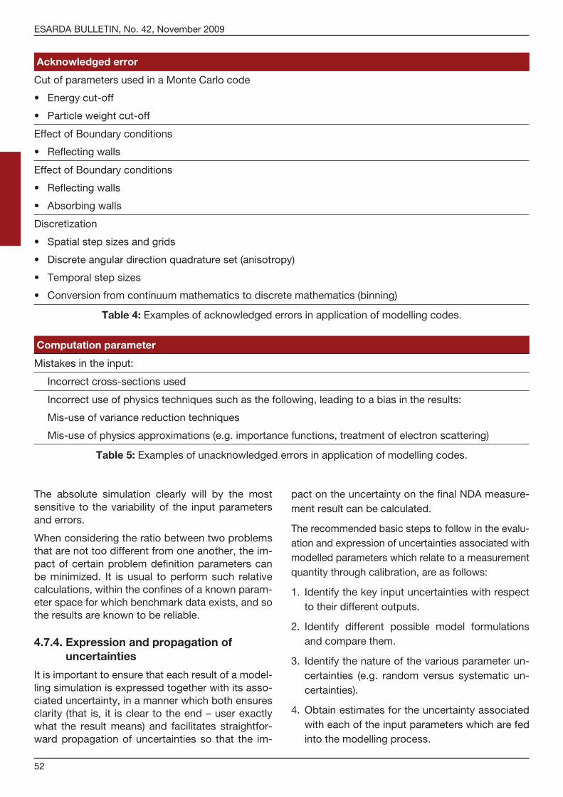
ESARDA BULLETIN, No. 42, November 2009
52
The absolute simulation clearly will by the most sensitive to the variability of the input parameters and errors.
When considering the ratio between two problems that are not too different from one another, the im-pact of certain problem definition parameters can be minimized. It is usual to perform such relative calculations, within the confines of a known param-eter space for which benchmark data exists, and so the results are known to be reliable.
4.7.4. Expression and propagation of uncertainties
It is important to ensure that each result of a model-ling simulation is expressed together with its asso-ciated uncertainty, in a manner which both ensures clarity (that is, it is clear to the end – user exactly what the result means) and facilitates straightfor-ward propagation of uncertainties so that the im-
pact on the uncertainty on the final NDA measure-ment result can be calculated.
The recommended basic steps to follow in the evalu-ation and expression of uncertainties associated with modelled parameters which relate to a measurement quantity through calibration, are as follows:
1. Identify the key input uncertainties with respect to their different outputs.
2. Identify different possible model formulations and compare them.
3. Identify the nature of the various parameter un-certainties (e.g. random versus systematic un-certainties).
4. Obtain estimates for the uncertainty associated with each of the input parameters which are fed into the modelling process.
Acknowledged error
CutofparametersusedinaMonteCarlocode
• Energycut-off
• Particleweightcut-off
Effect of Boundary conditions
• Reflectingwalls
Effect of Boundary conditions
• Reflectingwalls
• Absorbingwalls
Discretization
• Spatialstepsizesandgrids
• Discreteangulardirectionquadratureset(anisotropy)
• Temporalstepsizes
• Conversionfromcontinuummathematicstodiscretemathematics(binning)
Table 4: Examples of acknowledged errors in application of modelling codes.
Computation parameter
Mistakes in the input:
Incorrect cross-sections used
Incorrect use of physics techniques such as the following, leading to a bias in the results:
Mis-use of variance reduction techniques
Mis-use of physics approximations (e.g. importance functions, treatment of electron scattering)
Table 5: Examples of unacknowledged errors in application of modelling codes.

ESARDA BULLETIN, No. 42, November 2009
53
5. Determinetheeffectofeachinputuncertaintyonthe associated uncertainty in output quantity (for example, a detector tally).
Sensitivity studies are often used to determine the effect of an uncertain input parameter, on the un-certainty associated with the output parameter.
6. Determine the standard uncertainty for each pa-rameter.
7. Propagatethestandarduncertaintiesonthein-dividual model parameters, to determine the ef-fect on the instrument calibration parameter and ultimately the standard uncertainty on the final measurement quantity.
8. Apply theappropriatemultiplier toexpress thefinal result at the desired confidence level.
We present below, a formalism for expressing and propagating uncertainties, based on established practices[1,59and61].
The expression of the value of the result of a meas-urement or calculation, F, is incomplete without a statement of its evaluated uncertainty, U. This char-acterises the range in which the “true value” is esti-mated to lie with a given level of confidence. Any particular observation (i.e. measurement or calcula-tion) will then produce a sample value that lies somewhere within a defined probability distribution function at which the “true value” is usually located at the mod-point (for example in a Gaussian or “normal” distribution). It is important to understand the nature of the probability distribution function, because it is usually the confidence level that is of direct interest to the end-user.
Each parameter has an associated uncertainty i
that characterizes the spread of values within which the true value xi is believed to lie. If xi may lie any-where within a specified range of values with equal probability, it is said to have a rectangular probabil-ity distribution and the uncertainty is expressed in terms of the value for the semi-range. Alternatively, the probability distribution can be normal (i.e. Gaus-sian), and the standard deviation (or a given multi-ple of the standard deviation) may be used. An un-certainty should always be expressed in terms of a numerical value for an associated level of confi-dence. This obviously means that the type of the probability distribution should also be known. If the nature of a particular distribution is unknown, a conservative approach is to assume that it is a rec-tangular distribution, as this will lead to a conserva-tively high standard uncertainty value.
Table 6 summarises the common types of probabil-ity distribution functions that are relevant when cal-
culating uncertainties. The “divisor” gives the number by which the stated uncertainty parameter must be divided, to give the corresponding “stand-ard uncertainty” at a 67.7 % confidence level, equivalent to “one standard deviation”. When prop-agating uncertainties, one should use the standard uncertainty value for each parameter.
The combined standard uncertainty of the output quantity, u, is derived by the summation in quadra-ture of each of the individual standard uncertainty terms as shown in equation 7 (assuming that the terms are uncorrelated).
Guidance for procedures to propagate uncertainties canbefoundintheliterature[62,63,64,65,66,67and68].
Distribution Parameter Confidence level
Divisor (k)
Normal 1 standard deviation
67.7% 1.0
Normal 2 standard deviations
95.5% 2.0
Normal 3 standard deviations
99.7% 3.0
Rectangular semi-range 100% √3
Table 6:Commontypesofprobabilitydistributionfunctions.
The above expression applies only when the input quantities are independent of each other, i.e. when they are uncorrelated. Correlation analysis [61]should be used if this assumption does not hold. Furthermore, care may be required to allow for the non-normal behaviour of the “high end tail” of com-mon probability distributions.
When the standard uncertainty has been calculated, after propagating each of the individual terms, an appropriate multiplier or “coverage factor” should be applied so that the final uncertainty result is ex-pressed at the desired confidence level. The stand-ard uncertainty (multiplier of 1) equates to a confi-dence level of 67.7 %. If a multiplier of 2 is applied (equivalent to 2 standard deviations for a normal distribution) then the confidence level is 95.5%.Similarly, a multiplier of 3 gives a confidence level of 99.7 %. It is common, in NDA applications, to adopta95.5%confidencelevel(multiplierof2).Asimilar concept is applied as a coverage factor is needed to adjust the standard deviation for a small sample to represent a given confidence level for an infinite number of degrees of freedom (that is, the “students t distribution”).
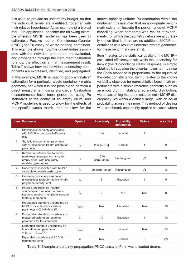
ESARDA BULLETIN, No. 42, November 2009
54
It is usual to provide an uncertainty budget, so that the individual terms are identified, together with their relative importance. As an example of a typical real – life application, consider the following exam-ple whereby MCNPmodelling has been used tocalibrate a Passive neutron CoincidenceCounter(PNCC)forPuassayofwaste-bearingcontainers.This example shows how the uncertainties associ-ated with the individual parameters are evaluated, and propagated through the instrument calibration to show the effect on a final measurement result. Table 7 shows how the individual uncertainty com-ponents are expressed, identified, and propagated.
Inthisexample,MCNPisusedtoapplya“relative”calibration for a particular waste container / matrix geometry, for which it is not possible to perform a direct measurement using standards. Calibrationmeasurements have been performed using Pustandards at the centre of an empty drum, and MCNPmodellingisusedtoallowfortheeffectsofthe specific waste matrix, and to allow for the
knownspatiallyuniformPudistributionwithin thecontainer. It is assumed that an appropriate bench-markexiststoillustratetheperformanceofMCNPmodelling, when compared with results of experi-ments, for which the geometry details are accurate-lyknown(thatis,therearenoadditionalMCNPun-certainties as a result of uncertain system geometry, for these benchmark systems).
Item1relatestothestatisticalqualityoftheMCNP–calculated efficiency result, while the uncertainty for item2(the“CoincidenceReals”response)issimplyobtained by squaring the uncertainty on item 1, since the Reals response is proportional to the square of the detection efficiency. Item 3 relates to the known variability observed for representative benchmark ex-periments with a simple reference geometry such as an empty drum. In stating a rectangular distribution, weareassumingthatthemeasurement/MCNPdis-crepancy lies within a defined range, with an equal probability across the range. This method of dealing with benchmark uncertainty applies to cases where
Item Parameter Symbol Uncertainty Probability distribution
Divisor ui ( ± % )
1 Statistical uncertainty associated withMCNP–calculatedefficiencytally
1 1 % Normal 1 1
2 Statistical uncertainty associated with“CoincidenceReals”calibrationparameter
2 2%[=2 1] Normal 1 2
3 Known uncertainty due to bench-mark experiment performance for empty drum, with accurately modeled geometries
315%
(semi-range)Rectangular √3 9
4 UncertaintyassociatedwithMCNP– calculated matrix perturbation 4 20 (semi-range) Rectangular √3 12
5 Geometry model approximation uncertainties (detector active length, polythene density, etc)
5 5 Gaussian 1 5
6 Physicsuncertainties(neutronsource spectrum, neutron cross-sections, neutron multiplicity second factorial moments)
6 0 N/A N/A 0
PropagatedstandarduncertaintyonMCNP–calculatedcalibrationparameter=( (i=1-6)ui
2 )0.5MCNP N/A Gaussian N/A 16
7 Propagatedstandarduncertaintyonmeasured calibration response parameterforPustandards
7 10 Gaussian 1 10
Expanded standard uncertainty on final calibration parameter =( MCNP
2+ CALIB2 )0.5
CALIB N/A Normal N/A 19
Expandeduncertaintyat95.5%confidence level
U N/A Normal 2 38
Table 7:Exampleuncertaintypropagation:PNCCassayofPuinwasteloadeddrums.

ESARDA BULLETIN, No. 42, November 2009
55
no benchmark exists for the as-built chamber. Alter-natively, it is sometimes possible to establish a benchmark for the as-build system, in which case a simple correction factor is applied to take account of the known measurement – modelled result bias. Sim-ilarly,item4referstotheuseofMCNPtocalculatetheperturbationeffectofadefinedmatrix.Item5re-fers to uncertainties due to the fact that the exact de-tails of the assay chamber are usually not known. Any additional uncertainties (item 6) from physics approx-imations and nuclear data, are neglected because in this example it is assumed that the same nuclear data is used, as for the benchmark systems (see item 3). The effects of uncertain nuclear data and physics ap-proximations are therefore already included in the uncertainty for item 3.
We see that the propagated standard uncertainty for the modelled response is 16 %, and in this case the individual terms have been added in quadrature because the individual items are multiplicative with regard to their contribution to the final calibration parameter. In this example the standard uncertainty on the measured calibration parameter, which equates to the count rate per unit mass of 240Puef-fective at the centre of an empty drum, is 10 %. The final calibration parameter (count rate per unit mass of 240Pueffectivedistributeduniformly throughoutthe matrix-loaded container) is therefore given by the product of the measured calibration parameter andtheMCNP-calculatedresponseexpressedasaratio to the empty drum “centre” position. This leads to a final uncertainty of 19 % at 67.7 % confidence, or38%at95.5%confidence(thatis,amultiplierof 2).
In the above example, we have presented a simpli-fied problem, in the sense that we have assumed each input parameter to be independent. For more complex problems, it may be necessary to fold the individualprobabilitydensityfunctions(PDF’s).
Furtherreadingmaybefoundinreferences[59,60,61, 62 and 63].
It is important to note that for real NDA applications it is not only the modelled parameters that must be taken into account when determining the uncertain-ty on a measured quantity. In practice there are various other factors which are not amenable to as-sessment using the techniques described in this guide, such as the following. These required careful consideration by experimentation.
• Effectsofpulsepile-upleadingtolossofpeakresolution.
• Deadtimelosses.
• Interference(toagammapeakofinterest)fromotherspecies(forexampleperformingPuisotop-ics measurements in the presence of a high gamma background from fission products).
• Abiasmayoccurifassumptionsthataremadeas part of the calibration, are not true (for exam-ple a sample is not, in practice, in true secular equilibrium).
• Electricalnoise.
• Temperature effects (drift) in the detector andamplifier.
• Dead layer growth (in Germanium detectors)which may alter the efficiency and invalidate the calibration.
• Physical changes such as moisture content,temperature, air pressure and humidity, seasonal neutron background variations, people moving in the vicinity of neutron counters (changing the moderation), etc.
5. Conclusions
The use of computer-based modelling tools is be-coming increasingly widespread in the support of Non Destructive Assay (NDA) measurements, both in the context of development of the techniques, and calibration of measurement equipment. The in-creasing availability of powerful computing systems is making this possible, whilst the availability of cali-brated nuclear material standards is diminishing. For these reasons, increasing reliance is being placed on the modelling tools. This means that it is becom-ing increasingly important to be able to demonstrate the validity of the results of modelling techniques, both to internal stakeholders and to regulators.
The specialist nature of the codes considered in this report(MonteCarlocodessuchasMCNP,MCBEND,KENO, Reactor Physics depletion codes such asFISPIN,ORIGEN, and ray-tracing analytical codessuchasISOCSandISOTOPIC)generallymeansthatexpert and experienced physicists are required to run the codes and interpret the results. This high-lights the importance of training and development / implementation of Quality Assurance procedures, to ensure that the codes are operated correctly, and within the known and documented operational range for the codes. However, the technical issues are complex, and require careful consideration to assess validity of modelling calculations.
This report considers each of the issues that must be considered to ensure reliable use of modelling codes in the field of NDA. Both technical (physics,

ESARDA BULLETIN, No. 42, November 2009
56
nuclear data, benchmarking, uncertainties, etc) and management (QA, training, etc) issues are consid-ered. We illustrate, through worked examples of real-life applications, how modelling codes are suc-cessfully used to calibrate NDA measurement sys-tems. This leads to identification of the key issues that determine the reliability and accuracy of mod-elling results, and suggestions for further work. We have shown how the correct use of modelling codes can lead to highly accurate calibrations of NDA sys-tems without relying on the use of physical stand-ards, provided that sound training and QA princi-ples are followed, and that strict benchmarking is followed. Benchmarking consists of ensuring the reliable performance of the modelling technique within a parameter space for which reliable valida-tions (comparing a measured with a modelled re-sult) exist. We have also shown the importance of a rigorous treatment of uncertainties, when assessing the results of computer modelling, and presented a formalism, consistent with established best practice for NDA measurements, for both expressing the modelling results and propagating the individual terms to show the impact on the final NDA meas-urement result.
It is concluded that the ultimate limit to the accura-cy to which modelling codes can be used to predict NDA system responses (which are not challenged by count rate and environmental factors), is deter-mined by the accuracy of the nuclear data which is used by the codes (for example half-lives, stopping powers, neutron spectra, neutron multiplicity data) and any subsequent interpretational models. This limits the accuracy with which codes can be used to make absolute predictions of count rates / sys-tem calibrations. However, when applied for relative calculations, provided that comprehensive and valid benchmarks are used to establish the predicted / measured response ratio, these biases can be re-moved through normalisation. There are many pub-lished benchmarks, however work is required in the NDA industry to maintain good benchmarks as NDA measurement techniques are being applied for more diverse nuclear material fuel types. A good exampleofthisistheuseofMonteCarlomodellingtechniques to calibrate neutron counting equipment for safeguards measurements of fissile material. Whilst at the present time the known nuclear data, used in combination with benchmark experiments, is sufficient, this will not necessarily be the case when new more exotic fuel types are becoming subjected to safeguards measurements. For these reasons, a high degree of emphasis should be placed on the continual evaluation and improve-ment of nuclear data.
In this report we describe each of the best practice topics highlighting the principles which if followed, will ensure reliable modelling results. It is hoped that this will be a useful guide for both modelling practitioners and other stakeholders including man-agement, regulators, and “intelligent customers”.
6. Glossary
The following terms are used in this document:
Analytical codes – Codes which use analyticaltechniques to model a radiation transport problem, based on using equations to model the effects of the sample material on the radiation transport.
Benchmarking – Measurements or experimental tests carried out under reference conditions to pro-duce results against which the results of measure-ments or tests carried out under other conditions may be compared.
Systematic Bias – A deviation that produces a consistent (repeatable) deviation from the true value in a given situation.
Burn-Up codes – See Reactor Physics Codes
Calibration –Proceduretoestablishaquantitativerelation between the response of an instrument and thequantity tobemeasured.Performedbyusinganalytical techniques, measurements or computer modeling involving one or more reference standards and / or validated computer codes and interpreta-tional models, under a set of reference conditions.
Calibration Factor – Reciprocal of response. Fac-tor by which a reading is multiplied to obtain the quantity being measured.
Central Limit Theorem – A statistical theorem which states that the sampling distribution curve that results from combining many independent var-iates will be centered on the population parameter value and it will have all the properties of a normal distribution.
Confidence Level – A number expressing the de-greeofconfidenceintheresult;usuallyexpressedas confidence band in terms of a percentage or as a number of standard deviations.
Coverage Factor – A number that is multiplied by the combined standard uncertainty to give an ex-panded uncertainty for a given confidence level.
Depletion Codes – See Reactor Physics Codes
Error – A deviation from the true value, normally brought about as a result of an incorrect or uncer-tain calculation or interpretation of a measurement.
ESARDA BULLETIN, No. 42, November 2009
57
Expanded Uncertainty – The standard uncertainty (or combined standard uncertainty) multiplied by a coverage factor for a given confidence level.
Gamma Spectrometry – A radiological assay tech-nique involving the identification and quantification of b/g radionuclides by analysis of the pulse height distribution (spectrum) recorded in a detector.
Hard modeling application – Sometimes also re-ferred to as Absolute. Refers to application of mod-eling tools where the modeling is used to directly calculate a result, without recourse to normalization against any measurement result.
Interpretational Model – An algorithm embodying a set of equations and approximations / assump-tions, that is used to convert calculated or meas-ured individual parameters, into a directly measur-able response parameter.
Matrix – The material surrounding or holding the substance being assayed. This material may signifi-cantly affect the response of the system by attenu-ation, absorption and other effects on radiation emerging from or entering the substance.
Measurand – A directly measured quantity.
Monte Carlo – A family of computer modeling codes that directly simulates the behaviour or parti-cles by modeling the physical scattering / absorp-tion behaviour, to predict the results of measurable quantities.
Non-Destructive Assay – The observation of spon-taneous or stimulated (induced) radioactive emis-sions, interpreted to estimate the amount of one or more nuclides of interest in the item being assayed, without affecting the physical or chemical form of the material, and without opening the container.
Passive Neutron Coincidence Counting – A tech-nique that counts bursts of neutrons, for example as time-correlated pairs, usually deployed in Non DestructiveAssaytoquantifyPu.
Passive Neutron Multiplicity Counting – A variant ofPassiveNeutronCoincidenceCountinginwhichdata on the number of neutrons detected together in a burst, is retained.
Precision – A measure of the reproducibility of a measurement / calculation result comprising contri-butions from repeatability of the measurement / cal-culation and random counting / modeling statistics.
Random uncertainty – The uncertainty for a pa-rameter for which an individual measured value lies within a distribution that contains the expectation
value formed over repeat measurements (Type A uncertainty).
Reals – The directly measured output quantity of a passive neutron coincidence counter based on shift register time analysis.
Reactor Physics Codes –Commonlyalsoreferredto as “Burn-up codes”, “Depletion codes” or “in-ventory codes”. Used to simulate the behaviour of materials in a reactor environment, and calculate the resulting inventory of radionuclides in the fuel / other reactor components.
Reference Standard – A physically and chemically stable item for which the attributes of interest are well-characterised and traceable to primary stand-ards, and for which the other properties affecting the measurement technique are known. Reference standards are used in a measurement system to establish the relationship between the basic instru-ment response and the attribute(s) of interest
Repeatability – Intrinsic instrument variability – a measure of the agreement between repeated meas-urements of the same quantity under unchanged conditions of measurement.
Reproducibility – A measure of the agreement be-tween repeated measurements of the same quantity under changed but replicated conditions of meas-urement.
Response – The ratio of the observed reading of an instrument to the true value of the quantity produc-ing that reading.
Soft modeling application – Sometimes also re-ferred to as Relative. Refers to application of mod-eling tools where the modeling is used to infer the result by taking ratios against directly measured quantities.
Standard Deviation – The positive square root of the variance.
Standard Uncertainty – Uncertainty of a measure-ment expressed as a margin equivalent to plus or minus one standard deviation.
Stochastic – Description of a process whereby the value is subject to inherent random variability.
Systematic uncertainty – An uncertainty that is represented by a constant bias or off-set, for a measured value compared to the true value under a given condition.
Total Measurement Uncertainty – A combination of the evaluated precision and bias terms, to ex-press the total uncertainty on a measurement or calculation result. The Total Measurement Uncer-

ESARDA BULLETIN, No. 42, November 2009
58
tainty is normally expressed at a defined confidence level,commonlyat95%.
Traceability – The ability to relate measurements to appropriate national or international standards through an unbroken chain of calibrations carried out in a technically sound manner.
Type A uncertainty – An uncertainty that can be evaluated using statistical means, from replicate measurements.
Type B uncertainty – An uncertainty that must be evaluated using non-statistical means.
Uncertainty –Parameter,associatedwiththeresultof a measurement, which characterises the disper-sion of the values that could reasonably be attrib-uted to the quantity being measured.
Variability – The inherent variation associated with the measurement / calculation system and its envi-ronment. Also refers to stochastic variations.
Variance – A term used to describe the dispersion of a set of observations with respect to its arithme-tic mean. Equal to the mean square deviation from the arithmetic mean.
The following acronyms and symbols appear in this document:
– Ratio of random-to-spontaneous fission neutron production rates for non-multiplying plutonium bearing material
AWCC –ActiveWellCoincidenceCounting:aneu-tron technique based on discriminating between neutrons from fission induced by an external source and the interrogating radiation (random neutrons). SometimesknownasANCC(ActiveNeutronCoin-cidence counting)
BWR – Boiling Water Reactor
CPU –CentralProcessingUnit
DG-TREN – Euratom Safeguards Inspection de-partment:
– Directorate General for Transport and Energy
DXTRAN – A technical term used in relation to a specific type of variance reduction featured within theMCNPcode.
ENDF – Evaluated Nuclear Data File
– Efficiency of detector system
FOM – Figure Of Merit
HEU – Highly Enriched Uranium (normally meaning having a 235U proportion greater than 20 %).
HPGe –HighPurityGermaniumusedforgamma-ray detection and energy measurement
IAEA – International Atomic Energy Agency
JEFF – Joint Evaluated Fission and Fusion File
JENDL – Joint Evaluated Nuclear Data Library
ILW – Intermediate Level Waste
FDET – Fork Detector Irradiated Fuel Measuring System
FORK – Safeguards detector used for spent fuel burnup measurement
JRC –JointResearchCentre
LLD – Lower Limit of Detection
LLW – Low Level Waste
LWR – Light Water Reactor
meff – Effective 240Pumassofplutonium (orothernuclear material)
ML – Neutron leakage multiplication
MOX – Mixed (plutonium and uranium) Oxide – a reactor fuel type
NaI(Tl) or NaI – Thallium-activated sodium iodide (a scintillator material used for gamma-ray detection and energy measurement)
NDA – Non Destructive Assay
NMA – Nuclear Material Accountancy
PDF –ProbabilityDensityFunction
PERLA – “Performance Laboratory” at Joint Re-searchCentre(JRC)/Ispra
PNCC –PassiveNeutronCoincidenceCounting:aneutron technique based on discriminating between time-correlated neutrons from spontaneous fission materials and single neutrons from other sources
PNMC –PassiveNeutronMultiplicityCounting:aneutron technique based on the measurement of singles, double coincidences and triple coincidenc-es of neutrons emitted from sample
PWR –PressurisedWaterReactor240Pueq or 240Pueff – 240Puequivalentmass(or240Pueffective mass)
R&D – Research and Development
SF – Spontaneous fission
SNF – Spent Nuclear Fuel
SNM – Special Nuclear MaterialtotalPu, totPu or Putotal – Total plutonium mass

ESARDA BULLETIN, No. 42, November 2009
59
TMU – Total Measurement Uncertainty
VLRM –VeryLowlevelRadioactiveMaterial
VOV –VarianceOftheVariance(atermusedinsta-tisticalanalysisofMonteCarlomodelingresults)
VVER –“Voda-VodyanoiEnergeticheskyReaktor”(RussianequivalentforPWRreactor)
The following established modeling and data analy-sis codes are cited in this document.
AMPX – Nuclear data / processing code
ANISN – Discrete ordinates radiation transport code
CEPXS – Discrete ordinates radiation transport code
CESAR –ReactorPhysicscode
DANTSYS – Discrete ordinates radiation transport code
DOORS – Discrete ordinates radiation transport code
DORT – Discrete ordinates radiation transport code
EGS4 –MonteCarlocode
FISPIN –ReactorPhysicscode
FLUKA –MonteCarlocode
FRAM – Gamma ray analysis code for plutonium and uranium isotopics assay
GAMMASHIELD – Software for calculating gamma ray attenuation
IGA – Software for the determination of actinides isotopics
ISOCS – Software for calculating gamma ray at-tenuation and gamma detector efficiencies
ISOTOPIC – Software for calculating gamma ray attenuation
ITS –MonteCarlocode
KENO –MonteCarlocode(usedforcriticalitycal-culations)
LAHET –MonteCarlocode
MCBEND –MonteCarlocode
MCNP –MonteCarlocode
MCNP-PTA –VariantofMCNPusedforsimulatingneutron pulse trains
MCNP-REN –VariantofMCNPusedforsimulatingNDA counting systems
MCNP-VISED –VisualisationsoftwareforMCNP
MERCURE – A dose-rate modelling program.
–Version6isdistributedbyCanberrathroughtheMERCURADhumangraphicalinterface.
MGA – Gamma ray analysis code used to deter-mine plutonium isotopics
MGA-U – Gamma ray analysis code used to deter-mine uranium isotopics
MONK –MonteCarlocode
MORSE –MonteCarlocode
NJOY – Nuclear data / processing code
ORIGEN –ReactorPhysicscode
PARTISN – Discrete ordinates radiation transport code
SCALE – Nuclear data / processing code
SOURCES – Nuclear data / processing code
TORT – Discrete ordinates radiation transport code
TRANSX – Nuclear data / processing code
TRIPOLI –MonteCarlocode
TWOTRAN – Discrete ordinates radiation transport code
References[1] P.McClellandandV.Lewis(Ed).NationalPhysicalLaboratory
MeasurementGoodPracticeGuideNo.34.RadiometricNon-DestructiveAssay.ISSN1368-6550,January2003.
[2] NumericalModellingConceptsforIAEASafeguards.ReportoftheCo-ordinatedTechnicalMeeting,IAEA,Vienna,19-21De-cember 2006.
[3] R.Venkataraman,,M.Villani,S.Croft,P.McClay,R.McElroy,S. Kane, W. Mueller, R. Estep. “An integrated Tomographic Gamma Scanning system for non-destructive assay of radio-activewaste”,Nucl. Inst.Meth. inPhys.Res.A579 (2007),375-379.
[4] MCNP–AGeneralMonteCarloN-ParticleTransportCode,Version5,LA-UR031987,LA-UR093,0425.
[5] R.Venkataraman,F.Bronson,V.Atrashkevich,B.M.Young,andM.Field.(CanberraIndustries,Meriden,CT.,USA).“Vali-dationofIn-SituObjectCountingSystem(ISOCS)mathemati-cal efficiency calibration software.” Presented at the NinthSymposium on Radiation Measurements and Applications, May11-14,1998AnnArbor,MI,USA.Alsopublished:NuclearInstrumentsandMethodsinPhysicsResearch(A),422(1999),pp.450-454.
[6] R.Venkataraman,F.Bronson,V.Atrashkevich,M.Field,andB.M.Young.“ImprovedDetectorResponseCharacterizationMethodinISOCSandLabSOCS”,JournalofRadioanalyticalandNuclearChemistry,Vol.264,No.1(2005),213-219
[7] W.F. Mueller, F. Bronson, M. Field, K. Morris, D. Nakazawa, R. Venkataraman,andV.Atrashkevitch.“Challengesandtech-niques to effectively characterize the efficiency of broad-ener-

ESARDA BULLETIN, No. 42, November 2009
60
gygermaniumdetectorsatenergieslessthan45keV”,PaperpresentedatMARC-VIII(MethodsandApplicationsofRadio-analytical Chemistry) conference, Hawaii, April 6-10, 2009, Accepted for publication in the Journal of Radioanalytical and NuclearChemistry(2009)
[8] MCBEND:AMonteCarloprogramforgeneralradiationtrans-portsolutions,ANSWERS/MCBEND(94)15,Answerssoftwareservice, Serco Assurance.
[9] J.P.Both,H.Derriennic,B.MorillonandJ.C.Nimal.“AsurveyofTRIPOLI-4”,Proceedingsofthe8thInternationalconferenceonRadiationShielding,Arlington, Texas,April 24-28, 1994,pp 373-377.
[10] GEANT website: http://geant4.cern.ch/support/userdocu-ments.shtml
[11]C.Suteau,M.ChironandG.Arnaud.ImprovementofMER-CURE-6’sgeneralformalismforcalculatinggamma-raybuild-up factors inmultilayershields.Nuc.Sci&Eng.147,43-55(2004).
[12] F.L. Bronson. “Three new techniques for radiological charac-terisationanddoseestimation”.Presentedattheinternationalconference: Decommissioning challenges: An Industrial Reali-ty.Sponsoredby IAEA,ENS,OECD/NEA,SFENNovember23-25,2003,Avignon,France
[13]H.Toubon,B.Nohl,S.Lefevre,M.Chiron,K.Boudergui,P.Pin.“Newmethodologyforsourcelocationandactivitydeter-mination in preparation of repairing or decommissioning ac-tivities”.IRPAconference,18may2006,Paris.
[14]A.G.Croff.ORIGEN2:AVersatileComputerCodeforCalculat-ing theNuclideCompositionsandCharacteristicsofNucle-arMaterials.NuclearTechnology,62,335-352(Sept.1983)
[15]SCALE: AModular Code System for Performing Standard-izedComputerAnalysesforLicensingEvaluations,ORNL/TM-2005/39,Version5.1,Vols.I-III,Nov.2006.
[16] International Nuclear Verification Series No. 1 “SafeguardsTechniques and equipment” 2003 Edition. International Atomic EnergyAgency,Vienna.
[17]H.Toubon,A.Lebrun,L.Oriol,NSaurel,T.GainandP.Pin.“Burn-up measurements coupling gamma spectrometry and neutronmeasurement”. ENC2005 conference, VERSAILLESDecember2005.
[18]M.Samsonetal.“CESAR:asimplifiedevolutioncodeappliedtoreprocessingapplication”.RECOD98,Nice(F)October25-28,1998
[19]J.M.Gomit,P.Cousinou,A.Duprey,C.Diop,J.P.Grouillier,L.Leyval,H.Toubon,E.Lejeune.“ThenewCRISTALcriticalitysafety package”. Sixth InternationalConference onNuclearCriticalitySafety,Versailles,France,20-24September1999(ICNC’99).
[20]D.J. Whalen, D.A. Cardon, J.L. Uhle and J.S. Hendricks.“MCNP:NeutronBenchmarkProblems”,LosAlamosNationalLaboratory, LA-12212, 1993
[21]D.J.Whalen,D.E.HollowellandJ.S.Hendricks.“MCNP:Pho-tonBenchmarkProblems”,LosAlamosNationalLaboratory,LA-12196, 1991.
[22]P.Baeten,M.Bruggeman,P.Chard,S.Croft,D.Parker,C.Zimmerman, M. Looman and S. Guardini. “Results of the ES-ARDA‘Reals’PredictionBenchmarkExercise”;ESARDABul-letin No. 31, (April 2002).
[23]P.Chardetal.“ResultsoftheESARDAMonteCarlo‘SimpleCase’BenchmarkExercise";ESARDABulletinNr32,(March2004).
[24]P.PeeraniandM.Swinhoe.“ResultsoftheESARDAMultipli-cityBenchmarkExercise”;ESARDABulletinNo.34.
[25]R.Venkataraman,F.Bronson,V.Atrashkevich,B.M.YoungandM.Field.“Validationof in-SituObjectCountingSystem(ISOCS)mathematical efficiency calculation software”, Pro-ceedings of the 9th Symposium on Radiation Measurements Applications,AnnArbor,MI,USA,May11-14,1998.
[26]R.Venkataraman,F.Bronson,V.Atrashkevich,B.M.YoungandM.Field.“Validationof in-SituObjectCountingSystem(ISOCS)mathematicalefficiencycalculationsoftware”,Nucl.InstandMethodsinPhysResA422(1999),pp450–454.
[27]P.Peerani,G.Bosler,I.CherradiandP.Schwalbach.“Com-putationalCalibrationofNeutronCollarsfortheVerificationofHEU Fuel Elements”, Proceeding of the 45th INMM Annual Meeting,Orlando(FL),18-22July2004.
[28]P.Peerani.“ComputationalcalibrationofUNCLneutroncol-lars for fresh fuel elements”, JRCTechnicalNote, I.04.142,October 2004.
[29]P.PeeraniandJ.Tanaka.“Calibrationofneutroncollarsforfresh fuel element verification”,Proceedingof the 27thES-ARDA Symposium on Safeguards and Nuclear Material Man-agement,London(UK),10-12May2005.
[30]P. Peerani. “Measurement of 235U in fresh WWER fuel ele-ments”,ProceedingsoftheTripartiteSeminar,Obninsk(RF),9-13 October 2006.
[31]H.Tagziria,P.Peerani,W.KoehneandP.Schwalbach.“On-LineVerificationofMOXFuelMagazinesUsingMonteCarloSimulation”,Proceedingofthe27th ESARDA Symposium on Safeguards and Nuclear Material Management, London (UK), 10-12May2005.
[32]H.Tagziria,P.Peerani,P.DeBaereandP.Schwalbach.“Mon-teCarloModellingandDesignOptimisationofaNeutronCo-incidenceCounterfortheVerificationofPuO2cans”,Proceed-ing of the 10thInternationalSymposiumonRadiationPhysics,Coimbra(PT),17-22September2006.
[33]P.Peerani,M.Looman:“ComputationalmodellingofNDAin-strumentsfornuclearsafeguards”,Proc.24th ESARDA Annual Meeting,Luxembourg,(June2002),or“MonteCarlosimula-tion of neutron counters for safeguard applications”, to be publishedonNucl.Instr.&Meth.inPhys.Res.A.
[34]A.LNichols,D.LAldamaandM.Verpelli.HandbookofNuclearDataforSafeguards,INDC(NDC)-0502(Jan.2007).
[35]R.B.Firestone(Ed)TableofIsotopes(8thEdition),JohnWiley&Sons,Inc(1996)
[36]LBNL Isotopes Project Nuclear Data Dissemination HomePage,http://ie.lbl.gov/toi.html
[37]M.Bergeretal.XCOM:PhotonCrossSectionDatabase,NIST,Gaithersburg, MD, USA, http://physics.nist.gov/xcom
[38]J.F. Ziegler. SRIM/TRIM computer code for calculation ofmass stopping powers of ions in matter. www.srim.org
[39]M.S.ZuckerandN.E.Holden.“ParametersforseveralPluto-nium Nuclides and 252CfofSafeguardsInterest”,Proc.6th ES-ARDAConf.,Venice(I),14-18May1984,341.
[40]ENDF-6FormatsManual.DataFormatsandProcedures fortheEvaluatedNuclearDataFileENDF/B-VIandENDF/B-VII.DocumentENDF-102,ReportBNL-NCS-44945-05.
[41] “Neutron reference radiations for calibrating neutron-measur-ing devices used for radiation protection purposes and for determining their response as a function of neutron energy”, InternationalStandardISO8529:1989(E).

ESARDA BULLETIN, No. 42, November 2009
61
[42]P.Schillebeeckx,M.LoomanandARavazzani.“Nucleardatarequired for non destructive assay of fissile and fertile materi-al”,Presentedattheseminaronfission,Pointd’Oye,Belgium,Sept. 1999 (A useful paper describing the benefits for NDA safeguards measurements, of obtaining improved nuclear data)
[43]D.M.Cifarelli,W.Hage.“Modelsforathreeparameteranaly-sis of neutron signal correlation measurements for fissile ma-terialassay”,Nucl.Instr.andMeth.A251,(1986),550-563.
[44]N.Ensslinetal.“ApplicationGuidetoMultiplicityCounting”,LA-13422-M,LosAlamos,(November1998).
[45]S.Croft,R.D.McElroyandS.C.Kane.Coincidencegateutili-sation factors for neutron correlation counters with up to three componentsinthedie-awayprofile.Proceedingsofthe11thInternationalConferenceonEnvironmentalRemediationandRadioactiveWasteManagement,ICEM2007,September2-6,2007, Oud Sint-Jan Hospital Conference Center, Bruges, Belgium.
[46] I.Pazsit,A.EnqvistandL.Pal.Anoteonthemultiplicityex-pressions in nuclear safeguards. Nucl. Inst and Methods in PhysResA603(2009),pp541–544.
[47]R.Gunnink.“MGA:AGamma-RaySpectrumAnalysisCodeforDeterminingPlutoniumIsotopicAbundances,Vol.1:Meth-odsandAlgorithms”,UCRL-LR-103220,Vol.1(1990).
[48]R.Gunnink,W.D.Ruther,P.Miller,J.Goerten,M.Swinhoe,H.Wagner,J.Verplancke,M.BickelandS.Abousahl.“MGAU:ANewAnalysis Code forMeasuringU-235 Enrichments inArbitrary Samples”, UCRL-JC-114713, Lawrence LivermoreNational Laboratory, (1994).
[49]T.E.Sampson,G.W.Nelson,T.A.Kelly. “FRAM:AVersatileCode for Analyzing the Isotopic Composition of Plutoniumfrom Gamma-Ray Pulse Height Spectra”, LA-11720-MS(1989).
[50] IGE:AnAutomaticsoftwareforthedeterminationofactinidesisotopicsabundances.ProceedingsoftheInternationalWork-shoponGammaSpectrometryAnalysiscodesforUandPuisotopics,OakRidge,Tennessee,USA,Nov03-07,2008.
[51]E.E.LewisandW.F.MillerJr.“Computationalmethodsofneu-trontransport”,Wiley-Interscience,NewYork,1984.
[52] I.LuxandL.Koblinger.“MonteCarloParticleTransportMeth-ods:NeutronandPhotonCalculations”,CRCPress,BocaRa-ton, 1991
[53]B.Morillon.“Unetechniquedebiaisageautomatique”,Proc.AdvancedMonteCarlocomputerprogramsforradiationtrans-port. Saclay (France) 27th April 1993.
[54]T.E. Booth. “A Sample Problem for Variance Reduction inMCNP”,LANLReportLA-10363-MS(10/1985).
[55]H.Tagziria,P.Peerani,W.KoehneandP.Schwalbach.“On-lineverificationofMOXFuelMagazinesinSMPwithD4detec-
tor”,Proceedingof the27thESARDASymposiumonSafe-guards and Nuclear Material Management, London (UK), 10-12 May2005.
[56]N.Roberts,H.TagziriaandD.Thomas.“DeterminationoftheeffectivecentresoftheNPLneutronlongcounters”,NPLre-port DQL RN004, Nov. 2004.
[57]W.L.Oberkampfetal.“EstimationofTotalUncertaintyinMod-ellingandSimulation”,SandiaReport,SAND2000-0824,April2000
[58]W.L.Oberkampfetal.“Verification,Validation,andPredictiveCapability in Computational Engineering and Physics”,SAND2003-3769, February 2003.
[59]UnitedKingdomAccreditationService,TheExpressionofUn-certaintyandConfidenceinMeasurement,UKASPublicationM 3003, Edition 1, 1997.
[60] [NASA] www.nianet.org/ecslectureseries/pdfs/isukapalli_030 405.pdf(NASA/NIAECSLectureSeries)
[61]PD6461:Part3:1995:VocabularyofMetrology,Part3.Guideto the expression of uncertainty in measurement, International Organisation for Standardisation, Geneva.
[62]ASTMstandardC1637“StandardTerminologyofC26.10Non-destructive Assay Methods”. See www.astm.org/Standards/C1637.htm. Nuclear, Solar and Geothermal Energy. ASTM BookofStandardsvolume12.01:Nuclearenergy(I)Publishedby:ASTMInternational,100BarrHarborDr,POBoxC700,W.Conshohocken,PA19428-2959.RevisionIssuedannually.
[63] ISO, International Organization for Standardization, Guide to the Expression of Uncertainty in Measurement, GUM, 1 Rue Varambé,CasePostale56,CH1221,Geneva,Switzerland.
[64] M. Grabe. Measurement Uncertainties in Science and Tech-nology. Springer. ISBN 3-540-20944-7, 2005. http://www.springer.com/dal/home/generic/search/results?SGWID=1-40109-22-24419924-0,2005.
[65]M.Grabe."PrinciplesofMetrologicalStatistics".Metrologia23(4):213–19.doi:10.1088/0026-1394/23/4/006.http://www.iop.org/EJ/article/0026-1394/23/4/006/metv23i4p213.pdf,1987.
[66] M. Grabe. "Estimation of Measurement Uncertainties—an Al-ternative to the ISO Guide". Metrologia 38 (2): 97–106.doi:10.1088/0026-1394/38/2/1. http://www.iop.org/EJ/arti-cle/0026-1394/38/2/1/me1201.pdf,2001.
[67] The Alternative Error Model and its Impact on Traceability and KeyComparison,JointBIPM-NPLWorkshopontheEvalua-tionofInterlaboratoryComparisonData,NPL,Teddington,19September 2002.
[68]DraftISOstandard:“Determinationofthecharacteristiclimits(decision threshold, detection limit and limits of the confidence interval) for measurements of ionizing radiation – Fundamen-tals and application”, International Standard ISO/DIS-11929, draft21/07/08.
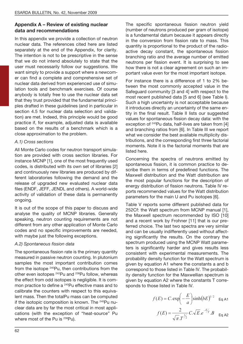
ESARDA BULLETIN, No. 42, November 2009
62
Appendix A – Review of existing nuclear data and recommendations
In this appendix we provide a collection of neutron nuclear data. The references cited here are listed separately at the end of the Appendix, for clarity. The intention is not to be prescriptive in the sense that we do not intend absolutely to state that the user must necessarily follow our suggestions. We want simply to provide a support where a newcom-er can find a complete and comprehensive set of nuclear data derived from experienced use of simu-lation tools and benchmark exercises. Of course anybody is totally free to use the nuclear data set that they trust provided that the fundamental princi-ples drafted in these guidelines (and in particular in section4.5 fornucleardata selectionandvalida-tion) are met. Indeed, this principle would be good practice if, for example, adjusted data is available based on the results of a benchmark which is a close approximation to the problem.
A.1) Cross sections
AllMonteCarlocodesforneutrontransportsimula-tion are provided with cross section libraries. For instanceMCNP[1],oneofthemostfrequentlyusedcodes, is distributed with its own set of libraries [2] and continuously new libraries are produced by dif-ferent laboratories following the demand and the release of upgraded new evaluated nuclear data files (ENDF, JEFF, JENDL and others). A world-wide activity of validation of these data is permanently ongoing.
It is out of the scope of this paper to discuss and analyse the quality of MCNP libraries. Generallyspeaking, neutron counting requirements are not differentfromanyotherapplicationofMonteCarlocodes and no specific improvements are needed, with maybe just the following exceptions.
A.2) Spontaneous fission data
The spontaneous fission rate is the primary quantity measured in passive neutron counting. In plutonium samples the most important contribution comes from the isotope 240Pu,thencontributionsfromtheother even isotopes 242Puand238Pufollow,whereasthe effect from odd isotopes is negligible. It is com-mon practice to define a 240Pueffectivemassandtocalibrate the counters with respect to this equiva-lentmass.ThenthetotalPumasscanbecomputedif the isotopic composition is known. The 240Punu-clear data are by far the most critical in most appli-cations (with the exception of “heat-source” PuwheremostofthePuis238Pu).
The specific spontaneous fission neutron yield (number of neutrons produced per gram of isotope) is a fundamental datum because it appears directly in the conversion from fission rate to mass. This quantity is proportional to the product of the radio-active decay constant, the spontaneous fission branching ratio and the average number of emitted neutrons per fission event. It is surprising to see how there is not a clear agreement on such an im-portant value even for the most important isotope.
For instance there is a difference of 1 to 2% be-tween the most commonly accepted value in the Safeguard community [3 and 4] with respect to the mostrecentpublisheddata[5and6](seeTableI).Such a high uncertainty is not acceptable because it introduces directly an uncertainty of the same en-tity in the final result. Table II lists our suggested values for spontaneous fission decay data: with the exception of 240Pudata,half-livesaretakenfrom[4]and branching ratios from [6]. In Table III we report what we consider the best available multiplicity dis-tributions, and the corresponding first three factorial moments. Note it is the factorial moments that are listed here.
Concerning the spectra of neutrons emitted byspontaneous fission, it is common practice to de-scribe them in terms of predefined functions. The Maxwell distribution and the Watt distribution are the most popular functions for the description of energydistributionoffissionneutrons.TableIVre-ports recommended values for the Watt distribution parametersforthemainUandPuisotopes[6].
TableVreportssomedifferentpublisheddata for252Cf:theWattspectrumfromMCNPmanual[1],the Maxwell spectrum recommended by ISO [10] and a recent work by Frohner [11] that is our pre-ferred choice. The last two spectra are very similar and can be usually indifferently used without affect-ing significantly the results. On the contrary the spectrumproducedusingtheMCNPWattparame-ters is significantly harder and gives results less consistent with experimental measurements. The probability density function for the Watt spectrum is given by equation A1 where the constants a and b correspondtothoselistedinTableIV.Theprobabil-ity density function for the Maxwellian spectrum is given by equation A2 where the constants T corre-spondstothoselistedinTableIV.
Eq A1
Eq A2

ESARDA BULLETIN, No. 42, November 2009
63
Reference Half-life (y) SF Branching ratio SF Half-life (y) Specific SF rate (s-1.g-1)
[3 and 4] 6560 5.65E-8 1.160E11 475
[5] 6568 5.70E-8 1.152E11 478
[6] 5.75E-8 1.141E11 485
Table I:Comparisonamongdifferentpublished240Puspontaneousfissiondata.
Isotope SF Half-life (y) Branching ratio SF (s-1) Spontaneous fission rate (.s-1.g-1)
238U 8.20E+15 5.45E-07 2.680E-24 6.776E-03238Pu 4.77E+10 1.84E-09 4.605E-19 1.165E+03239Pu 5.48E+15 4.40E-12 4.008E-24 1.010E-02240Pu 1.15E+11 5.70E-08 1.906E-19 4.791E+02241Pu 2.50E+15 5.74E-15 8.786E-24 2.195E-02242Pu 6.84E+10 5.50E-06 3.232E-19 7.989E+02241Am 1.05E+14 4.13E-12 2.092E-22 5.226E-01252Cf 85.6 3.092E-2 2.566E-10 6.130E+11
Table II: Suggested values for spontaneous fission decay data.
238U 238Pu 240Pu 242Pu 252Cf
References [7] [3, 9] [8] [8] [8]
P(0) 0.0782 0.0541 0.0655 0.0683 0.0021
P(1) 0.2465 0.2054 0.2319 0.2302 0.0260
P(2) 0.3563 0.3802 0.3289 0.3343 0.1267
P(3) 0.2363 0.2248 0.2514 0.2469 0.2734
P(4) 0.0719 0.1079 0.1015 0.0991 0.3039
P(5) 0.0101 0.0276 0.0184 0.0181 0.1848
P(6) 0.0006 - 0.0024 0.0031 0.0657
P(7) - - - - 0.0154
P(8) - - - - 0.0020
s1 2.0097 2.2100 2.1563 2.1450 3.757
s2 1.6066 1.9783 1.9121 1.8971 5.983
s3 0.6369 0.9327 0.8894 0.8863 5.302
Table III: Multiplicity distributions for spontaneous fission.
Isotope Watt spectrum parameters
a (MeV) b (MeV-1)238U 0.6483 6.811238Pu 0.8478 4.169240Pu 0.7949 4.689242Pu 0.8192 4.367
Table IV: Suggested Watt parameters for spontaneous fission neutron spectra.
Reference Distribution a (MeV) b (MeV-1) T (MeV)
[1] Watt 1.025 2.926 -
[10] Maxwell - - 1.420
[11] Watt 1.175 1.040 -
Table V:Comparisonamongdifferentpublisheddataon252Cf.

ESARDA BULLETIN, No. 42, November 2009
64
In passive neutron coincidence counting (PNCC),where the measured quantity is the coincidence “Reals” count rate, no distinction is made between the different (even numbered) spontaneously fission-ing isotopes. Measurement results are therefore normally expressed in terms of a 240Pu effectivemass, meff, where appropriate coefficients are de-fined to allow for the contribution from each of the even isotopesofPu, tomeff. The coefficients (see equation A3) depend on the nuclear data compris-ing of the spontaneous fission rate (s-1.g-1) and the second moment of the spontaneous fission neutron multiplicity distribution (that is, the parameter S2 with reference to equation 2 in section 4.5.2.1).These nuclear data are the subject of evaluation by experiment. A review paper [12] describes the evalu-ation of these parameters. Direct measurement of isotopically pure 238Puand242Pustandardsisapow-erful method of direct measurement of the meff coef-ficients. Such an exercise has been conducted [13, 14], which yielded coefficients of 2.71 and 1.66 (the values for A and B for 238Puand242Purespectively.An important point here is the need to use a consist-ent set of coefficients, in order to achieve consistent results (for example for series of verification inspec-tions). In terms of absolute nuclear data, however, it may still be worthwhile pursuing the determination, by measurement, of more accurate data.
Eq A3
A.3) Neutron-induced fission data
Beyond the cross sections, other nuclear data are required for a complete modelling of the induced fission reaction: the multiplicity distributions and the secondary neutron spectra. For the application of the point model it is enough to know just the aver-age neutron yield and the factorial moments of the multiplicity distribution.
What makes things more difficult than in the case of spontaneous fission is that the above said quanti-ties are not constant, but depend from the incident neutronenergy.Completemultiplicitydistributionsfor neutron induced fission (as a function of neutron energyupto10MeV)areavailablejustfor235U, 238U and 239Pu [15].TableVI resumes thedistributionsjust for En=0(thermal)and1MeV.Asfarassec-ondary neutron spectra are concerned, Table VIIwas derived from [1].
A.4) (alpha,n) reaction data
To compute the factor appearing in the point mod-el, we need to know the specific neutron yield from ( ,n) reaction. This is the number of neutrons per second produced in a gram of a determined isotope. To produce a neutron the alpha particle from the de-cay of an actinide must interact with a light target nuclide (oxygen, fluorine, beryllium or others). There-fore the neutron yield is not simply a property of the alpha emitter, but also of the matrix of the material and sometimes it depends on the presence of impu-rities.InTableVIIIwereportthespecific( ,n) neutron yieldsinuraniumandplutoniumoxides.Valuesavail-able in literature [16, 17 and 4] are compared with thosecomputedusingtheSOURCES-4Acode[18].
ForMonteCarlomodelling it isnecessary toknowalso the spectrum of emitted neutrons. Differently from fission neutrons, there is not a simple paramet-ric analytical expression for ( ,n) neutron spectra. Neutron spectra from ( ,n) reactions computed with SOURCES-4AforseveralplutoniumisotopesinoxidematrixarelistedinhistogramforminTableIX.Inthecase of the AmLi source used for active neutron in-terrogation the theoretical spectrum computed by Geiger and van der Zwan [19] seem still to be a rea-sonably good model. The GvdZ spectrum is given in TableX.Experimentallymeasuredspectrapublishedmore recently [20] could produce some improve-ments in the simulation. It is important to remark that the GvdZ spectrum is a theoretical spectrum of gen-erated neutrons, its use is recommended when the detailed description of the source is available (mate-rial,composition,density,geometry); inthiswayallthe modifications due to the neutron interactions with the source itself will be correctly taken into account. Experimentally measured spectra include already this information and are best suitable when the composi-tionofthesourceisnotknown;moreovertheycanaccount for effects due to spurious reactions such as ( ,n) on oxygen or impurities as beryllium. When us-ing escaping neutron spectra it would be better not to model the source: leave the source location void and let neutrons be generated at the source surface.
References [21, 22 and 23] provide worthwhile ad-ditional reading, providing neutron spectral data from robust measurements of Am/Li and Am/F ( ,n) neutron sources.
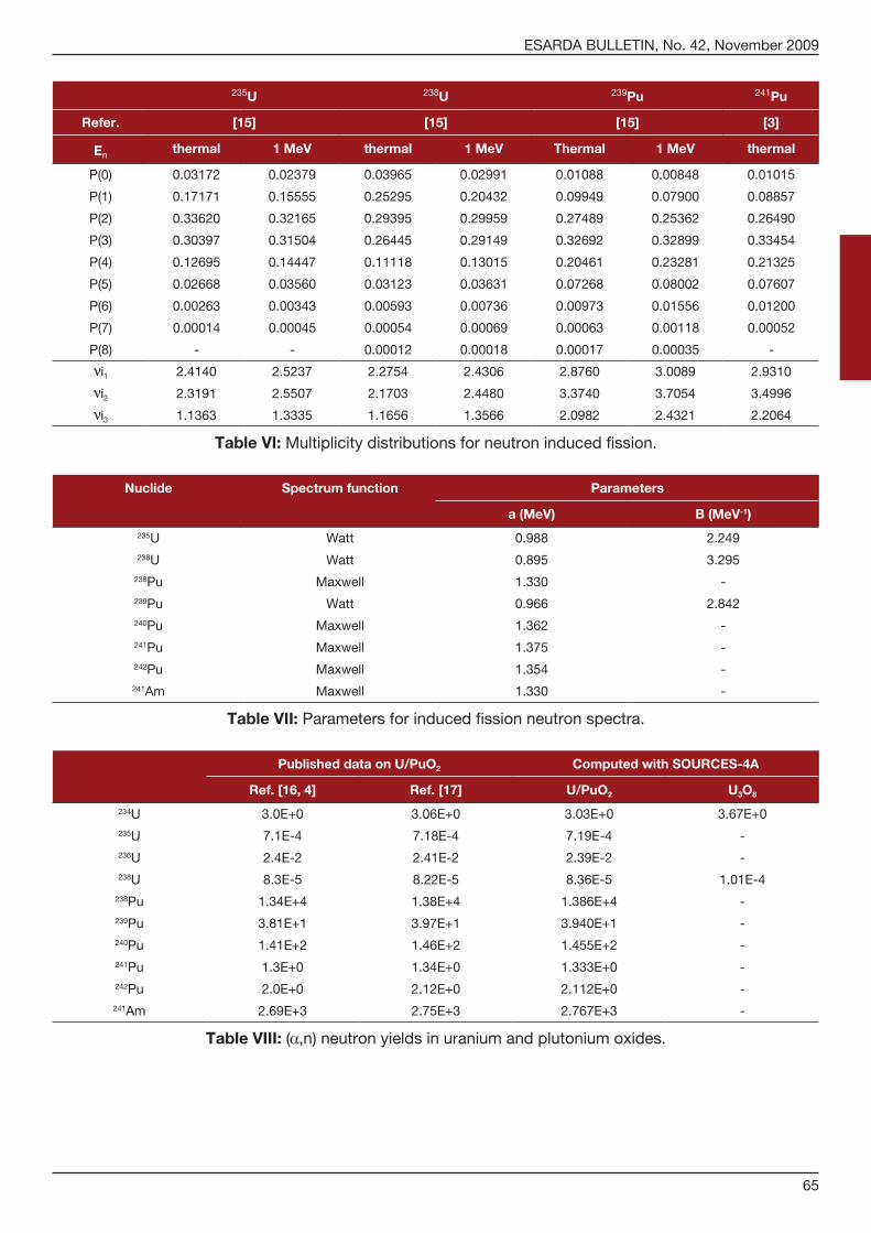
ESARDA BULLETIN, No. 42, November 2009
65
235U 238U 239Pu 241Pu
Refer. [15] [15] [15] [3]
En thermal 1 MeV thermal 1 MeV Thermal 1 MeV thermal
P(0) 0.03172 0.02379 0.03965 0.02991 0.01088 0.00848 0.01015
P(1) 0.17171 0.15555 0.25295 0.20432 0.09949 0.07900 0.08857
P(2) 0.33620 0.32165 0.29395 0.29959 0.27489 0.25362 0.26490
P(3) 0.30397 0.31504 0.26445 0.29149 0.32692 0.32899 0.33454
P(4) 0.12695 0.14447 0.11118 0.13015 0.20461 0.23281 0.21325
P(5) 0.02668 0.03560 0.03123 0.03631 0.07268 0.08002 0.07607
P(6) 0.00263 0.00343 0.00593 0.00736 0.00973 0.01556 0.01200
P(7) 0.00014 0.00045 0.00054 0.00069 0.00063 0.00118 0.00052
P(8) - - 0.00012 0.00018 0.00017 0.00035 -
i1 2.4140 2.5237 2.2754 2.4306 2.8760 3.0089 2.9310
i2 2.3191 2.5507 2.1703 2.4480 3.3740 3.7054 3.4996
i3 1.1363 1.3335 1.1656 1.3566 2.0982 2.4321 2.2064
Table VI: Multiplicity distributions for neutron induced fission.
Nuclide Spectrum function Parameters
a (MeV) B (MeV-1)235U Watt 0.988 2.249238U Watt 0.895 3.295238Pu Maxwell 1.330 -239Pu Watt 0.966 2.842240Pu Maxwell 1.362 -241Pu Maxwell 1.375 -242Pu Maxwell 1.354 -241Am Maxwell 1.330 -
Table VII:Parametersforinducedfissionneutronspectra.
Published data on U/PuO2 Computed with SOURCES-4A
Ref. [16, 4] Ref. [17] U/PuO2 U3O8
234U 3.0E+0 3.06E+0 3.03E+0 3.67E+0235U 7.1E-4 7.18E-4 7.19E-4 -236U 2.4E-2 2.41E-2 2.39E-2 -238U 8.3E-5 8.22E-5 8.36E-5 1.01E-4238Pu 1.34E+4 1.38E+4 1.386E+4 -239Pu 3.81E+1 3.97E+1 3.940E+1 -240Pu 1.41E+2 1.46E+2 1.455E+2 -241Pu 1.3E+0 1.34E+0 1.333E+0 -242Pu 2.0E+0 2.12E+0 2.112E+0 -241Am 2.69E+3 2.75E+3 2.767E+3 -
Table VIII: ( ,n) neutron yields in uranium and plutonium oxides.

ESARDA BULLETIN, No. 42, November 2009
66
Energy boundaries (MeV)
5.00 4.95 4.90 4.85 4.80 4.75 4.70 4.65
4.60 4.55 4.50 4.45 4.40 4.35 4.30 4.25
4.20 4.15 4.10 4.05 4.00 3.95 3.90 3.85
3.80 3.75 3.70 3.65 3.60 3.55 3.50 3.45
3.40 3.35 3.30 3.25 3.20 3.15 3.10 3.05
3.00 2.95 2.90 2.85 2.80 2.75 2.70 2.65
2.60 2.55 2.50 2.45 2.40 2.35 2.30 2.25
2.20 2.15 2.10 2.05 2.00 1.95 1.90 1.85
1.80 1.75 1.70 1.65 1.60 1.55 1.50 1.45
1.40 1.35 1.30 1.25 1.20 1.15 1.10 1.05
1.00 0.95 0.90 0.85 0.80 0.75 0.70 0.65
0.60 0.55 0.50 0.45 0.40 0.35 0.30 0.25
0.20 0.15 0.10 0.05 0.00238Pu 1.69E-04 1.79E-04 1.85E-04 1.92E-04 1.99E-04 2.07E-04 2.16E-04 2.25E-04
2.37E-04 2.51E-04 3.30E-04 6.13E-04 9.54E-04 1.30E-03 1.65E-03 2.00E-03
2.36E-03 2.73E-03 3.27E-03 3.84E-03 4.55E-03 5.33E-03 6.11E-03 6.77E-03
7.43E-03 8.16E-03 8.84E-03 9.57E-03 1.05E-02 1.11E-02 1.18E-02 1.26E-02
1.34E-02 1.43E-02 1.53E-02 1.62E-02 1.69E-02 1.76E-02 1.82E-02 1.90E-02
1.98E-02 2.09E-02 2.19E-02 2.23E-02 2.25E-02 2.26E-02 2.27E-02 2.30E-02
2.35E-02 2.36E-02 2.33E-02 2.31E-02 2.28E-02 2.23E-02 2.20E-02 2.17E-02
2.08E-02 1.98E-02 1.89E-02 1.83E-02 1.75E-02 1.70E-02 1.62E-02 1.51E-02
1.39E-02 1.32E-02 1.26E-02 1.20E-02 1.14E-02 1.07E-02 9.90E-03 9.42E-03
8.65E-03 8.02E-03 7.80E-03 7.28E-03 6.83E-03 6.49E-03 6.19E-03 6.07E-03
5.80E-03 5.49E-03 5.42E-03 5.29E-03 5.31E-03 5.14E-03 5.02E-03 5.05E-03
5.12E-03 5.04E-03 4.96E-03 4.77E-03 4.34E-03 4.18E-03 4.18E-03 4.17E-03
4.18E-03 3.74E-03 2.96E-03 1.85E-03239Pu 1.23E-04 1.35E-04 1.44E-04 1.52E-04 1.60E-04 1.71E-04 1.83E-04 1.94E-04
2.09E-04 2.28E-04 2.45E-04 2.70E-04 2.89E-04 3.03E-04 3.17E-04 3.37E-04
3.64E-04 6.39E-04 1.03E-03 1.24E-03 1.61E-03 2.04E-03 2.48E-03 2.79E-03
3.21E-03 4.07E-03 4.96E-03 5.90E-03 7.02E-03 7.85E-03 8.72E-03 9.77E-03
1.08E-02 1.19E-02 1.33E-02 1.44E-02 1.53E-02 1.61E-02 1.69E-02 1.79E-02
1.90E-02 2.04E-02 2.16E-02 2.25E-02 2.34E-02 2.42E-02 2.50E-02 2.57E-02
2.62E-02 2.66E-02 2.68E-02 2.70E-02 2.72E-02 2.68E-02 2.63E-02 2.59E-02
2.48E-02 2.34E-02 2.23E-02 2.15E-02 2.05E-02 1.99E-02 1.88E-02 1.75E-02
1.60E-02 1.50E-02 1.43E-02 1.35E-02 1.28E-02 1.18E-02 1.08E-02 1.02E-02
9.26E-03 8.61E-03 8.48E-03 7.94E-03 7.27E-03 6.49E-03 5.82E-03 5.57E-03
5.16E-03 4.71E-03 4.56E-03 4.35E-03 4.37E-03 4.14E-03 4.00E-03 4.03E-03
4.25E-03 4.61E-03 5.02E-03 5.32E-03 5.18E-03 5.06E-03 5.06E-03 4.99E-03
4.86E-03 4.20E-03 3.15E-03 1.81E-03240Pu 1.26E-04 1.37E-04 1.46E-04 1.54E-04 1.63E-04 1.73E-04 1.85E-04 1.96E-04
2.11E-04 2.29E-04 2.47E-04 2.71E-04 2.90E-04 3.04E-04 3.19E-04 3.37E-04
3.91E-04 7.04E-04 1.10E-03 1.31E-03 1.67E-03 2.10E-03 2.54E-03 2.85E-03
3.33E-03 4.21E-03 5.09E-03 6.02E-03 7.14E-03 7.97E-03 8.83E-03 9.87E-03
1.09E-02 1.20E-02 1.33E-02 1.44E-02 1.54E-02 1.61E-02 1.70E-02 1.79E-02
1.90E-02 2.04E-02 2.16E-02 2.25E-02 2.34E-02 2.42E-02 2.50E-02 2.57E-02
2.62E-02 2.66E-02 2.67E-02 2.69E-02 2.71E-02 2.66E-02 2.61E-02 2.57E-02
2.46E-02 2.33E-02 2.22E-02 2.14E-02 2.04E-02 1.98E-02 1.87E-02 1.74E-02
1.59E-02 1.50E-02 1.42E-02 1.35E-02 1.27E-02 1.18E-02 1.08E-02 1.02E-02
9.24E-03 8.59E-03 8.46E-03 7.92E-03 7.22E-03 6.44E-03 5.83E-03 5.58E-03
5.18E-03 4.73E-03 4.59E-03 4.39E-03 4.41E-03 4.18E-03 4.04E-03 4.07E-03
4.29E-03 4.64E-03 5.06E-03 5.35E-03 5.17E-03 5.04E-03 5.04E-03 4.96E-03
4.83E-03 4.17E-03 3.13E-03 1.80E-03
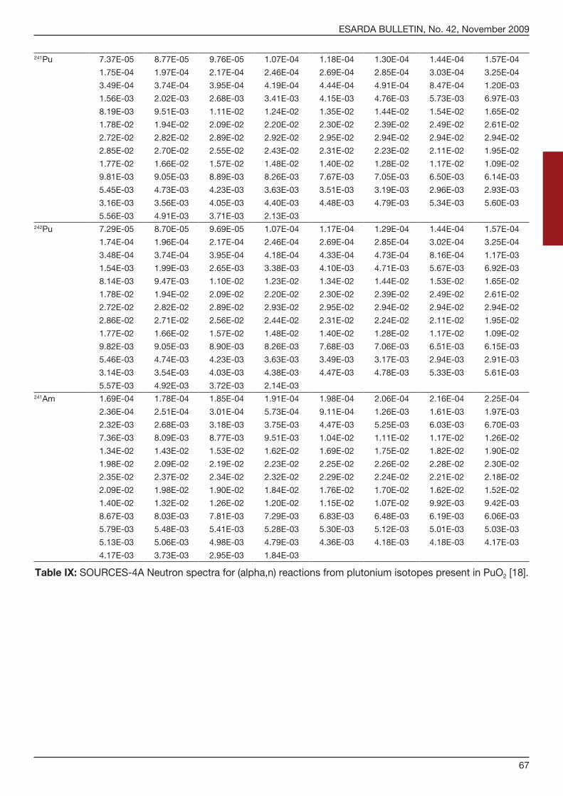
ESARDA BULLETIN, No. 42, November 2009
67
241Pu 7.37E-05 8.77E-05 9.76E-05 1.07E-04 1.18E-04 1.30E-04 1.44E-04 1.57E-04
1.75E-04 1.97E-04 2.17E-04 2.46E-04 2.69E-04 2.85E-04 3.03E-04 3.25E-04
3.49E-04 3.74E-04 3.95E-04 4.19E-04 4.44E-04 4.91E-04 8.47E-04 1.20E-03
1.56E-03 2.02E-03 2.68E-03 3.41E-03 4.15E-03 4.76E-03 5.73E-03 6.97E-03
8.19E-03 9.51E-03 1.11E-02 1.24E-02 1.35E-02 1.44E-02 1.54E-02 1.65E-02
1.78E-02 1.94E-02 2.09E-02 2.20E-02 2.30E-02 2.39E-02 2.49E-02 2.61E-02
2.72E-02 2.82E-02 2.89E-02 2.92E-02 2.95E-02 2.94E-02 2.94E-02 2.94E-02
2.85E-02 2.70E-02 2.55E-02 2.43E-02 2.31E-02 2.23E-02 2.11E-02 1.95E-02
1.77E-02 1.66E-02 1.57E-02 1.48E-02 1.40E-02 1.28E-02 1.17E-02 1.09E-02
9.81E-03 9.05E-03 8.89E-03 8.26E-03 7.67E-03 7.05E-03 6.50E-03 6.14E-03
5.45E-03 4.73E-03 4.23E-03 3.63E-03 3.51E-03 3.19E-03 2.96E-03 2.93E-03
3.16E-03 3.56E-03 4.05E-03 4.40E-03 4.48E-03 4.79E-03 5.34E-03 5.60E-03
5.56E-03 4.91E-03 3.71E-03 2.13E-03242Pu 7.29E-05 8.70E-05 9.69E-05 1.07E-04 1.17E-04 1.29E-04 1.44E-04 1.57E-04
1.74E-04 1.96E-04 2.17E-04 2.46E-04 2.69E-04 2.85E-04 3.02E-04 3.25E-04
3.48E-04 3.74E-04 3.95E-04 4.18E-04 4.33E-04 4.73E-04 8.16E-04 1.17E-03
1.54E-03 1.99E-03 2.65E-03 3.38E-03 4.10E-03 4.71E-03 5.67E-03 6.92E-03
8.14E-03 9.47E-03 1.10E-02 1.23E-02 1.34E-02 1.44E-02 1.53E-02 1.65E-02
1.78E-02 1.94E-02 2.09E-02 2.20E-02 2.30E-02 2.39E-02 2.49E-02 2.61E-02
2.72E-02 2.82E-02 2.89E-02 2.93E-02 2.95E-02 2.94E-02 2.94E-02 2.94E-02
2.86E-02 2.71E-02 2.56E-02 2.44E-02 2.31E-02 2.24E-02 2.11E-02 1.95E-02
1.77E-02 1.66E-02 1.57E-02 1.48E-02 1.40E-02 1.28E-02 1.17E-02 1.09E-02
9.82E-03 9.05E-03 8.90E-03 8.26E-03 7.68E-03 7.06E-03 6.51E-03 6.15E-03
5.46E-03 4.74E-03 4.23E-03 3.63E-03 3.49E-03 3.17E-03 2.94E-03 2.91E-03
3.14E-03 3.54E-03 4.03E-03 4.38E-03 4.47E-03 4.78E-03 5.33E-03 5.61E-03
5.57E-03 4.92E-03 3.72E-03 2.14E-03241Am 1.69E-04 1.78E-04 1.85E-04 1.91E-04 1.98E-04 2.06E-04 2.16E-04 2.25E-04
2.36E-04 2.51E-04 3.01E-04 5.73E-04 9.11E-04 1.26E-03 1.61E-03 1.97E-03
2.32E-03 2.68E-03 3.18E-03 3.75E-03 4.47E-03 5.25E-03 6.03E-03 6.70E-03
7.36E-03 8.09E-03 8.77E-03 9.51E-03 1.04E-02 1.11E-02 1.17E-02 1.26E-02
1.34E-02 1.43E-02 1.53E-02 1.62E-02 1.69E-02 1.75E-02 1.82E-02 1.90E-02
1.98E-02 2.09E-02 2.19E-02 2.23E-02 2.25E-02 2.26E-02 2.28E-02 2.30E-02
2.35E-02 2.37E-02 2.34E-02 2.32E-02 2.29E-02 2.24E-02 2.21E-02 2.18E-02
2.09E-02 1.98E-02 1.90E-02 1.84E-02 1.76E-02 1.70E-02 1.62E-02 1.52E-02
1.40E-02 1.32E-02 1.26E-02 1.20E-02 1.15E-02 1.07E-02 9.92E-03 9.42E-03
8.67E-03 8.03E-03 7.81E-03 7.29E-03 6.83E-03 6.48E-03 6.19E-03 6.06E-03
5.79E-03 5.48E-03 5.41E-03 5.28E-03 5.30E-03 5.12E-03 5.01E-03 5.03E-03
5.13E-03 5.06E-03 4.98E-03 4.79E-03 4.36E-03 4.18E-03 4.18E-03 4.17E-03
4.17E-03 3.73E-03 2.95E-03 1.84E-03
Table IX:SOURCES-4ANeutronspectrafor(alpha,n)reactionsfromplutoniumisotopespresentinPuO2[18].

ESARDA BULLETIN, No. 42, November 2009
68
Energy bounda-ries(MeV)
1.0E-11 0.001 0.002 0.003 0.004 0.005 0.006
0.007 0.008 0.009 0.01 0.02 0.03 0.04
0.05 0.06 0.07 0.08 0.09 0.1 0.11
0.12 0.13 0.14 0.15 0.16 0.17 0.18
0.19 0.2 0.22 0.24 0.26 0.28 0.3
0.32 0.34 0.36 0.38 0.4 0.42 0.44
0.46 0.48 0.5 0.52 0.54 0.56 0.58
0.6 0.62 0.64 0.66 0.68 0.7 0.72
0.74 0.76 0.78 0.8 0.82 0.84 0.86
0.88 0.9 0.92 0.94 0.96 0.98 1
1.02 1.04 1.06 1.08 1.1 1.12 1.14
1.16 1.18 1.2 1.22 1.24 1.26 1.28
1.3 1.32 1.34 1.36 1.38 1.4 1.44
1.48 1.5 1.52 1.54
Spectrum in histogram form (MeV-1)
0 0.00004 0.00007 0.00009 0.00011 0.00013 0.00014
0.00015 0.00017 0.00018 0.00019 0.00247 0.00352 0.00460
0.00585 0.00723 0.00852 0.00966 0.01055 0.01130 0.01187
0.01242 0.01292 0.01332 0.01343 0.01333 0.01322 0.01311
0.01297 0.01284 0.02542 0.02493 0.02448 0.02404 0.02355
0.02308 0.02261 0.02215 0.02173 0.02119 0.02071 0.02034
0.01978 0.01935 0.01894 0.01844 0.01803 0.01758 0.01715
0.01676 0.01626 0.01590 0.01552 0.01511 0.01471 0.01435
0.01401 0.01363 0.01329 0.01294 0.01263 0.01230 0.01201
0.01171 0.01141 0.01110 0.01082 0.01051 0.01022 0.00995
0.00963 0.00933 0.00902 0.00868 0.00835 0.00796 0.00759
0.00718 0.00677 0.00632 0.00591 0.00550 0.00509 0.00467
0.00428 0.00387 0.00346 0.00305 0.00267 0.00228 0.00332
0.00174 0.00032 0.00003 0.00000
Table X: Geiger and van der Zwan spectrum of the AmLi neutron source [19].

ESARDA BULLETIN, No. 42, November 2009
69
References for Appendix A [1] J.F.Briesmeister.“MCNP–AGeneralMonteCarloN-Particle
TransportCode”,LA-13709-M,LosAlamos(March2000).
[2] RSICCDataLibraryCollection.“MCNPDATA:StandardNeu-tron,PhotonandElectronDataLibrariesforMCNP4C”,DLC-200, Oak Ridge (March 2001).
[3] M.S.ZuckerandN.E.Holden.“ParametersforseveralPluto-nium Nuclides and 252CfofSafeguardsInterest”,Proc.6th ES-ARDAConf.,Venice(I),14-18May1984,341.
[4] D.Reilly,N.Ensslin,H.SmithJr.andS.Kreiner.“PassiveNon-destructive Assay of Nuclear Materials”, NUREG/CR-5550,LA-UR-90-732, (March 1991).
[5] JEFF2.2EvaluatedNuclearDataFile,(July1993).
[6] E.F.Shores.“DataUpdatesfortheSOURCES-4AComputerCode”,LA-UR-00-5016,LosAlamos,(October2000).
[7] M.R.Looman,P.PeeraniandP.Schillebeeckx.“AnOverviewofNDA Instrumentsmodelledwith theMCNP-PTACodeatJRCIspra”,Proc.23rdESARDAConf.,Bruges(B),8-10May2001.
[8] J.W.BoldemanandM.G.Hines.“PromptNeutronEmissionProbabilitiesfollowingSpontaneousandThermalNeutronFis-sion”,NuclearScienceEngineering,91,(1985),114.
[9] D.A.Hicks,J.IseandR.V.Pyle.“ProbabilitiesofPrompt-Neu-tron Emission from Spontaneous Fission”, Physical Review101,(1956),1016.
[10] “Neutron reference radiations for calibrating neutron-measur-ing devices used for radiation protection purposes and for determining their response as a function of neutron energy”, InternationalStandardISO8529:1989(E).
[11] F.H. Frohner. “Evaluation of 252CfPromptFissionNeutronDatafrom0to20MeVbyWattspectrumfit”,NuclearScienceEngi-neering,106,(1990),345-352.
[12]P.M.J.ChardandS.Croft.“Adatabaseof240Pueffectiveand235Ueffective coefficients for various fertile and fissile isotopes”. Proceedingsofthe19thESARDASymposiumonSafeguards&NuclearMaterialManagement,Montpellier,France,13-15May1997.
[13]H.Ottmar,P.vanBelle,S.Croft,P.M.J.Chard,L.C-A.Bourvaand U. Blohm-Hieber. “An Empirical Measurement of the Spe-cific240Pu-EffectiveMassof238Puand242Pu”.Proceedingsof the 21st ESARDA Symposium on Safeguards & NuclearMaterial Management, Sevilla, Spain, 4-6 May 1999.
[14]S.Croft,L.C-ABourva,D.R.WeaverandH.Ottmar.“240PuEffectiveMass of 238Pu and 242Pu in Relation to PassiveNeutron Coincidence andMultiplicity Counting”. Journal ofNuclearMaterialsManagement.Volume30(1),2001.
[15]M.S.ZuckerandN.E.Holden.“NeutronMultiplicityforNeu-tron Induced Fission of 235U, 238U and 239PuasaFunctionofNeutronEnergy”,IAEA-SM-293/122,Vienna(1986),329.
[16]R.T.PerryandB.W.Wilson. “NeutronProduction from ( ,n) Reactions and Spontaneous Fission in ThO2, UO2and(U,Pu)O2Fuels”,LA-8869-MS,LosAlamos,(June1981).
[17]S.Croft.“ThecalculationoftheEnhancementofthe( ,n)Pro-ductionRateinPuO2andMOXpowderscausedbythePres-enceofMoisture”,Proc.17thESARDAConf.,Aachen(D),9-11May1995,419.
[18]W.B.Wilsonetal.“SOURCES-4A:aCodeforcalculating( ,n), Spontaneous Fission and Delayed Neutron Sources and Spec-tra”, LA-13639-MS, Los Alamos, (September 1999).
[19] K.W. Geiger and L. van der Zwan. “The Neutron Spectra and theresultingFluence-kermaConversionsfor241Am-Li( ,n) and 210Po-Li( ,n)Sources”,HealthPhysics,21(1971)120-123.
[20] H. Tagziria, N.J. Roberts and D.J. Thomas. “Measurement of the 241Am–Li radionuclide neutron source spectrum”, Nuclear Instruments and Methods in Physics Research Section A,Vol.510,Issue3,(September2003),346-356.
[21] J.G. Owen, D.R. Weaver and J. Walker. “The calibration of a 3He spectrometer and its use to measure the spectrum of neutrons from an Am/Li source”. Nuclear Instrumentation and Methods.188(1981),579-593.
[22] D.R. Weaver, J.G. Owen and J. Walker. “The neutron spec-trumfroma5CiAm/Lineutronsource”.NuclearInstrumenta-tionandMethods.198(1982),599-602
[23] J.G. Owen, D.R. Weaver and J. Walker. “Neutron spectra from Am/F and Am/Li ( ,n) sources”. International conference on Nuclear Data for Science and Technology, Antwerp, 6-10 Sept (1982),492-495.

The cover of this Issue is inspired by its title ‘Non-Destructive Analysis’. It shows an image that seems to have a second layer on top, or looks like a mirror, but in fact it is not. It means ‘modifying a picture without destroying it’, an artistic translation of the Bulletin’s title.
