ta tuan anh computer aided taxi dispatching
TRANSCRIPT

Ta Tuan Anh COMPUTER AIDED TAXI DISPATCHING. SPECIFICATION OF THE SYSTEM. Thesis CENTRIA UNIVERSITY OF APPLIED SCIENCES Degree Programme in Information Technology December 2015

ABSTRACTS Department Kokkola-Pietarsari
Date December 2015
Author Ta Tuan Anh
Degree programme Information Technology Name of thesis COMPUTER AIDED TAXI DISPATCHING. SPECIFICATION OF THE SYSTEM. Instructor Dr. Grzegorz Szewczyk
Pages 74 + 9 appendices
Academic supervisor Dr. Grzegorz Szewczyk Company supervisor Ville H.S Ranta Taxi is one of the most important transporters in the public. However, how to make the taxi services more efficient in order to benefit not only taxi owners but also taxi drivers is one of the most interesting questions recently, especially when other competitors in this service are becoming more and more. In the current situation, there is no suggested service that drivers can rely on, which would recommend the highly possible pickup point that will most likely to have the customers at the particular time and location. At the moment, taxi drivers only believe in their routines to go to the station that is believed to have awaiting customers. Therefore, the idea of building a solution which can have a logical suggestion for drivers could be a promising project, that will satisfy not only taxi owners but also drivers and customers. The aim of the thesis is going to find a general solution in order to make the idea becoming real. Besides, some interesting topic such as the machine learning technique and neural network are also the main parts of the thesis as they were selected as the solution for the problem.
Key words optimization, neural network, requirements engineering, algorithm selection, taxi

CONTENTS 1. INTRODUCTION ........................................................................................................ 1 2. DESCRIPTION OF THE PROBLEM ....................................................................... 2
2.1. Current market ...................................................................................................................... 2 2.2. New approach for the improvement of the dispatching system ........................................ 4
3. SOLUTIONS FOR THE NEW PROPOSED APPROACH ..................................... 5 3.1. Description of the problem solving process ........................................................................ 5 3.2. Thesis objectives .................................................................................................................... 5 3.3. Thesis questions ..................................................................................................................... 6
4. SOFTWARE SPECIFICATION AND ARCHITECTURE ..................................... 7 4.1. Specific Requirements ........................................................................................................... 7
4.1.1. Functional requirements ...................................................................................................... 7 4.1.2. Non-functional requirements ............................................................................................ 11
4.2. Use Cases .............................................................................................................................. 17 4.3. Software Architecture ......................................................................................................... 20 4.4. Summary .............................................................................................................................. 21
5. DECOMPOSITION OF THE PROBLEM .............................................................. 22 5.1. Analyze the problem ........................................................................................................... 22 5.2. Solutions for sub-problems ................................................................................................. 22
5.2.1. List all the pickup points in a given distance limit. .......................................................... 22 5.2.2. Estimate the distance between the current input location and each suggested point. ....... 23 5.2.3. Estimate the travel time between the current input location and each suggested point. ... 24 5.2.4. Anticipate the number of customers at each point in case the driver arrives. ................... 24 5.2.5. Get the current number of taxis at each pickup point. ...................................................... 25 5.2.6. Calculate the percentage of reliability of each point, and display for users. .................... 26 5.2.7. Navigation for user after the selection. ............................................................................. 27
5.3. Summary .............................................................................................................................. 27 6. SELECTION OF PREDICTIVE MODELLING .................................................... 28
6.1. Options for predictive modelling ....................................................................................... 28 6.2. Classification and Regression Trees vs. Neural Networks .............................................. 30
6.2.1. Classification and Regression Trees (CART) ................................................................... 30 6.2.2. Neural Networks ............................................................................................................... 30 6.2.3. Comparison table and final selection ................................................................................ 31
6.3. Summary .............................................................................................................................. 32 7. NEURAL NETWORK ............................................................................................... 33
7.1. Introduction to Neural Networks ....................................................................................... 33 7.1.1. Basic concept .................................................................................................................... 33 7.1.2. Mathematical model of Neural Network .......................................................................... 35 7.1.3. Applicability of Artificial Neural Network ....................................................................... 38
7.2. Feed-forward Neural Networks ......................................................................................... 40 7.2.1. Single-layer Perceptron Neural Networks ........................................................................ 40 7.2.2. Multi-layer Perceptron Neural Networks .......................................................................... 42
7.3. Some issues to consider when using MLP networks ........................................................ 50 7.3.1. Standardization of input data ............................................................................................ 50 7.3.2. Under fitting and over fitting in learning process of the network ..................................... 51 7.3.3. Choosing a suitable network size ...................................................................................... 53
7.4. Combination of Genetic Algorithm and Back-propagation to optimize the weights in Neural Network ................................................................................................................................. 53 7.5. Genetic Algorithms .............................................................................................................. 54

7.5.1. The main idea of a genetic algorithm ................................................................................ 54 7.5.2. Diagram of a simple Genetic Algorithm ........................................................................... 56
7.6. Application of genetic algorithms to the optimization problem of the weight of the artificial neural network ................................................................................................................... 58
7.6.1. Construction of cost function ............................................................................................ 58 7.6.2. Encoding of chromosomes ................................................................................................ 58 7.6.3. Crossover .......................................................................................................................... 60 7.6.4. Mutation ............................................................................................................................ 61
7.7. Combining genetic algorithm and back propagation algorithm to optimize error weighting artificial neural network ................................................................................................. 62
7.7.1. Question ............................................................................................................................ 62 7.7.2. Combining genetic algorithm and back-propagation algorithm ....................................... 62
7.8. Summary .............................................................................................................................. 63 8. CREATING MATHEMATICAL MODEL OF NEURAL NETWORK IN THE OPTIMISATION OF THE CASE OF TAXI DISPATCHING. ......................................... 64
8.1. Mathematical Model Diagram ........................................................................................... 64 8.2. Preparation of input data ................................................................................................... 65
8.2.1. Departure location ............................................................................................................. 66 8.2.2. Departure date ................................................................................................................... 66 8.2.3. Departure time ................................................................................................................... 66 8.2.4. Climate Features ............................................................................................................... 66 8.2.5. Events near by / Public holidays ....................................................................................... 67 8.2.6. Real collected data ............................................................................................................ 68
8.3. Indicators to assess the results forecast ............................................................................. 70 8.4. Summary .............................................................................................................................. 71
9. CONCLUSIONS ......................................................................................................... 72 10. REFERENCES ............................................................................................................ 74 APPENDICES ........................................................................................................................... 1
TABLE OF FIGURES FIGURE 1. Example of the application which supports taxi ordering service ........................... 3 FIGURE 2. Design mockup of the main page of the application with mobile view .................. 8 FIGURE 3. Design mockup of the application after clicking a particular pickup point. ........... 9 FIGURE 4. Software Usability Measurement Inventory, SUMI. (Porteous et al. 1993) ......... 14 FIGURE 5. Principal properties of dependability. (Bev Littlewood, Lorenzo Strigini. 2014) . 15 FIGURE 6. Application Activities Use Case diagram .............................................................. 17 FIGURE 8. System architecture from building a machine learning software. (Xavier
Amatriain, Justin Basilico, 2013) ...................................................................................... 20 FIGURE 9. Category of colors for the reliability display ......................................................... 27 FIGURE 10. Microsoft Azure Machine Learning: Algorithm Cheat Sheet. (Microsoft Azure,
2016) ................................................................................................................................. 29 FIGURE 11. Example of a CART (Hemant Ishwaran and J. Sunil Rao. 2009). ...................... 30 FIGURE 12. The simulation of neural network in Machine Learning ..................................... 31 FIGURE 13. Structure of a typical neuron ............................................................................... 34 FIGURE 14. Artificial Neural Networks model (Nikola K. Kasabov, 1998). .......................... 34

FIGURE 15. Neural Networks with only one node and one feedback connection (Sima Jiri, 1998) ................................................................................................................................. 37
FIGURE 16. Single layer feed-forward network (Sima Jiri, 1998) .......................................... 37 FIGURE 17. Multi-layer feed-forward network (Sima Jiri, 1998) ........................................... 37 FIGURE 18. Single layer recurrent network (Sima Jiri, 1998) ................................................ 38 FIGURE 19. The difference between Linear Regression and Neural Networks Regression.
(Sima Jiri, 1998) ................................................................................................................ 39 FIGURE 20. Single-layer Perceptron Neural Networks. (Nikola K. Kasabov, 1998) ............. 41 FIGURE 21. The implementation of XOR function using MLP .............................................. 43 FIGURE 22. Spread signals in the learning process by the method of back-propagation
algorithm. (Nikola K. Kasabov, 1998) .............................................................................. 44 FIGURE 23. Error E is considered as a function of the weight W (Nikola K. Kasabov, 1998)
........................................................................................................................................... 45 FIGURE 24. Inertia in reality ................................................................................................... 50 FIGURE 25. Sigmoid function g(x) = 1/(1+e-x) ....................................................................... 51 FIGURE 26. Top: Polynomial fit to data from y = sin(x/3) + v, 0 ≤ x ≤ 20. Order 20 overfits.
Bottom: Small and large MLPs fit to same data. The large MLP does not overfit significantly more than the small MLP. (R. Caruana, S. Lawrence, Lee Giles. 2000) ..... 52
FIGURE 28. Flowchart of a simple Genetic Algorithm. (Brian R. West, Seppo Honkanen. 2005) ................................................................................................................................. 57
FIGURE 29. Binary encoding of weights using Genitor algorithm. ........................................ 59 FIGURE 30. Example of real number encoding of weights (D. Whitley. 1995) ..................... 60 FIGURE 31. Crossover-nodes (D. Montana and L. Davis, 1989) ............................................ 61 FIGURE 31. Diagram of the mathematical model in the optimization of taxi dispatching case.
........................................................................................................................................... 65 FIGURE 33. Example of AllEvent.in interface with the request for events in Helsinki in
March 2016 ....................................................................................................................... 68 FIGURE 34. Sample of statistic data for trips .......................................................................... 68
TABLE 1. Functional requirements for the application ........................................................... 10 TABLE 2. Response Time: The 3 important limits (Jakob Niesel. 2009). ............................... 12 TABLE 3. Time Scales in User Experience (Jakob Niesel. 2009). .......................................... 13 TABLE 4. User Registration ..................................................................................................... 18 TABLE 5. Display list of optimized stations ............................................................................ 19 TABLE 7. Evaluation of possible selected predictive modelling (Scottge, 2015) ................... 29 TABLE 8. Comparison between Neural Network and CART. ................................................ 31 TABLE 8. Table of sample of collected data from trips ........................................................... 68 TABLE 9. User Login ................................................................................................................. 1 TABLE 10. User setting ............................................................................................................. 1 TABLE 11. Select Language ...................................................................................................... 2 TABLE 12. Update username, password .................................................................................... 2 TABLE 13. Voice control system ............................................................................................... 3 TABLE 14. Input location .......................................................................................................... 3 TABLE 15. Use current location ................................................................................................ 4 TABLE 16. Get direction to go to the selected station ............................................................... 4 TABLE 17. Display statistic data ............................................................................................... 5

GRAPH 1. The demonstration of locations on the map as a 2D graph. ................................... 23

1
1. INTRODUCTION
For decades, taxi has become one of the most common and indispensable public transportation despite the development of trains and buses. However, it has always been a hard issue on how to make the taxi services more efficient in order to benefit not only taxi owners but also taxi drivers, especially when there are more and more competitors in the taxi market. In the current situation, there is no suggested service that drivers can dependably rely on, a service that would recommend the highly possible pickup point that will most likely to have the customers at a particular time and location. At the moment, taxi drivers only believe in their routines to go to the station that is believed to have awaiting customers. Therefore, the idea of building a solution which can have a logical suggestion for drivers could be a promising project, that will satisfy not only taxi owners but also drivers and customers. The aim of the thesis is going to find a general solution in order to actualize the idea. Besides, some interesting topics such as machine learning technique and neural network algorithms are going to be thoroughly discussed in the thesis as they have been selected as the solutions to the problem. Last but not least, the thesis will also mention about the prospect of further developments for the system, and other features that can be added in the next versions.

2
2. DESCRIPTION OF THE PROBLEM
According to the current situation of the taxi market, and what has been analyzed above, a new system has been proposed as it would be a system that facilitates the taxi dispatching system, but with end users including drivers and taxi company. In detail, it suggests the number of customers at the stands so that the end users can select the next pickup point according to their locations. Besides, the system will not display the real consumption but instead, suggest the predicted values according to the historical data and some other related figures.
2.1. Current market
The idea of “Taxi” has been introduced since the 17th century, and Taxi is still considered one of the most important transports for the public nowadays. There have been many improvements on the dispatching system, which can facilitate customers to find the nearest taxis in the area, and are undoubtedly helping people to order a taxi nearby. Compare to the last decades, when technology was not as modern as now, the only best way to get a taxi is to either call the taxi operator or to go to the nearest stand. Nowadays, there are many famous applications in the market that can help people to select a taxi by simple clicks. Some popular global apps can be listed here, such as TaxiFinder powered by TaxiFareFinder.com, Easy Taxi powered by EasyTaxi.com or some local apps like: Menevä for Helsinki area, etc. The common idea of the above-mentioned applications is that it is available in some specific regions (in 86 cities across 26 countries in the case of Easy Taxi) and allows users to quickly scrub through maps and find locations that they would like to be picked up at. After that, the users can confirm the ride and then pay for it within the application. Once the ride is booked, the taxi's plate number and phone number is given and appeared on the map as well, making it easy for the users to pick out both the car and the driver.

3
FIGURE 1. Example of the application which supports taxi ordering service
However, the common approach of the idea above came from the real time consumption of the customers, and drivers are impassive, as they have to wait for the order before making a move. Moreover, it is apparent that these application mainly supports the customers who want to order taxicabs, as it suggests the location of available cars for the customers and allows them to order from the system. A new question which brings a new approach is that is there a vice versa way which can support the taxi companies by giving them the location of the customers so that either taxi companies can distribute their cars or drivers can go to the higher consumed places?

4
2.2. New approach for the improvement of the dispatching system
As mentioned above, the new approach is somehow against the common idea at the moment: the idea comes from the support for taxi companies instead the support for customers. However, the particular tasks need to be defined. First of all, in the new system, the end users are drivers or taxi companies. Secondly, what the new system is capable of is that it should be able to display the locations which have customers at a given time to the drivers or companies. Besides, some additional features can be added such as the navigation system, etc. Considering the benefit of the new approach, drivers will always be passive, as they can always find from the system which place they should go after a completed trip. Also, from the taxi company’s point of view, they can reduce the fuel cost when their cars have to travel to find the customers. Besides, the company will be able to avoid the case of some low income cars, as the cars can always be distributed to the locations that have customers suggested from the system.

5
3. SOLUTIONS FOR THE NEW PROPOSED APPROACH
3.1. Description of the problem solving process
Although the new idea was clear, the next question is how to implement the idea into a real system? Is it a feasible feature in which the system can suggest the number of consumers? There are two possibilities of the solution, and each needs to be analyzed: the suggestion comes from the real consumption at the given time or the suggestion comes from the prediction
a. Real consumption at the given time
In order to get the real consumption at the given time, the system must be able to collect the orders at that moment. However, how can the system perform that task? The only answer is that it has to wait for the orders from customers, and shows it to the users (drivers or taxi companies). By doing this way, it comes back to the old approach: wait for the orders before making the decision. Therefore, this is not a good solution.
b. Prediction of data
Due to the fact that the suggestion is just a prediction, it will not be absolutely precise. However, according to the modern algorithm, and the intelligence of science nowadays, it is possible to predict data (number of customers in this case) according to the historical data. In terms of predicting values, there are several possibilities that can solve the trick by using physical model, mathematic model or machine learning technique. Overall, in order to create the system, the suggestion based on predicted values is a good way to implement. It is apparently not easy to build a predicting system, especially when the predicted values (number of customers in each stand) is non-linear, and depends on many other predicted values (weather, traffic, etc.). However, to start building the application, the specifications have to be defined at the beginning. The thesis is going to be a part of that, and therefore, it is necessary to find the objectives and questions for this thesis.
3.2. Thesis objectives
The objective of the thesis is to analyze the specification of the system, such as the requirements engineer, the selection of mathematical model. Besides, the thesis is also going to decompose the big problem into sub-problems according to the requirements engineer and the selection of the mathematical model. However, the thesis will not go deeply in detail of how to solve all issues, but instead, more focus on the decision making of the solution for each sub-problem.

6
3.3. Thesis questions
According to the research objectives, the research question should be: • What are software specifications of the project? • What are the sub-problems of the project? • What are the solutions for these sub-problems? • What is the mathematical model in the optimization of taxi dispatching system?

7
4. SOFTWARE SPECIFICATION AND ARCHITECTURE
All systems involve interaction. In a software system context, these interactions might be user interaction, which has to do with user inputs and outputs, or interaction between different components of the system and even interaction between different systems. Modelling user interaction uncovers and describes the User requirements. (Sommerville 2010, 124.) Modelling the system component interaction helps to comprehend and validate System requirements based on performance and dependability. Modelling system-to-system interaction sheds light on the communication problems that may arise between the proposed system and system it may have to communicate with. (Sommerville 2010, 124.) Therefore, this chapter is going to present the functional and non-functional requirements first. Use case diagram is also going to be presented next, in order to clearly describe the user requirements (functional requirements, in particular).
4.1. Specific Requirements
Software requirements are the descriptions of what a system or software should do, that is, the services it should provide and the limitations on its operations. These requirements reveal the needs of customers or users for system or software that serves a certain purpose or solves a certain technology problem such as controlling a device, editing text or placing an order. Requirements engineering (RE) is the process of finding out, analyzing, documenting and checking software or system’s services and constraints. (Sommerville 2010, 83.)
4.1.1. Functional requirements
The application has 13 main requirements. These requirements are the basis for the system function. Firstly, like any other application which requires the authentication process, the application will have a login system, which authenticate users before using the app. After the authentication and authorization, the application should know the basic information of the driver such as the taxi owner information, where the driver belongs to, the car which is now driven by the driver, basic information of drivers (name, email, phone – editable data), etc. Secondly, no matter if the application is developed as a web app or mobile app, it should have a navigation mechanism, which can navigate the current position of the user in order to suggest a correct place. In the next requirement, due to the fact that the suggestion is mainly based on the input location, it could be any location which contains a precise longitude and latitude data, and therefore, users will be allowed to not only find the next pickup point by the current location but also can find by manually input the desired address. Fourthly, the result will be displayed as a list of suggested places (at the beginning stage, the application will support filter by distance only), so that users can decide the next proper pick up

8
place, as in some cases, the best suggested place will not be an ideal destination for them by considering some external reasons. For example, it could be the last trip in the shift, so that the drivers prefer to drive in some places close to their homes (these reasons can not be taken as a parameter in the algorithm of the application). Moreover, by giving some real-time extra information such as the distance, and time to travel to each pickup point (including the possibility of facing traffic jams, etc. by using a third party API), the application will basically give more options for users to define the concept of “best possible pickup place”, and by their consideration, they can find their best places. However, apart from the distance and travel time, the main purpose of the application is to give the anticipated number of available customers at each point at the time the driver is supposed to arrive at the location, and therefore, the number of anticipated customers as well as the ratio of the number of customer and the available taxis (in percentage %) will be displayed in the application. The higher the percentage is, the darker the background is colored. Figure 1 shows how the main interface and function of the application work.
FIGURE 2. Design mockup of the main page of the application with mobile view

9
In detail, in order to give the suggested pickup points sorted by distance, there is a need to have a distance boundary so that the application can circulate all the point in the circle area and make calculations for these point. Therefore, the application must have the possibility to allow users to input the limited distance, or the application will have a default limited distance. Nevertheless, the application will be built in such a smart way that when the user scrolls the page down, it will automatically extend the radius by a particular number (1km, for example), and retrieve more suggestions. After clicking the suggested place, users should be redirected to a map or GPS navigation page, which will guide them how to reach the destination. It could be a part of the application or could also be passed as a parameter to another GPS application (Google maps, Apple maps or Bing maps) as long as it works automatically. Otherwise, users have to remember the address, and retype it in another navigation app (which is too complicated and requires a lot of work in user’s point of view).
FIGURE 3. Design mockup of the application after clicking a particular pickup point.

10
Besides, voice control is something that can considerably attract users, especially in this case when drivers must use their hand to control the car. In reality, if voice control is implemented successfully, it would make the application become more pragmatic and helpful. For instance, users can command the application to find the list of suggestion with their given address, etc. The voice control can be integrated by utilizing the voice recognition system from the operating system itself such as Siri for iOS or Mac OS, Cortana for Windows OS or Windows Phone OS, or Google Voice for Android OS. (As the artificial intelligence world becomes more and more developed, voice recognition is becoming significantly reliable, and is something that developers should extremely pay attention to) (Matthew Baxter-Reynolds. 2011). According to the fact that taxi drivers in Finland come from various countries, and not all of them can speak Finnish professionally, there is a need to support a multilingual system. Hence, the system should be build to support multilingual application, and allow end users to opt their languages. Besides, for the marketing purpose, statistic functionality should also be an interesting part, as it can be used to show to the end users how much money that he or she has been benefited by using this optimization system. The registration process is also important. However, due to the security issue, the creation of new driver users should only be done by the system administrator or the taxi owner user level, so that the system will be fully controlled. In the long run, social network login should also be taken into account, as social network is one of the most popular system, which has all the basic user info nowadays. Last but not least, the possibility to support the application as a cross-platform application or even a web API is also a crucial feature. With a well-organized back-end system, the application can be developed in many different interface (independent software, integrated software, API), so that it can approach users widely and easily. Table 1 illustrates shows the list of functional requirements for the application. TABLE 1. Functional requirements for the application
Functional requirements
1. The application shall have a login system, which allows driver to authenticate him or herself.
2. Users shall be allowed to change their settings such as username, password, basic contact information, etc. However, some critical info, for example, taxi owner info, driver number, car number are strictly prohibited, at least for the normal user level.
3. The application shall have a navigation system, which can find the current location of authenticated user. Based on the location, the application can give a correct suggestion for users.
4. Users shall be able to find the suggested place based on the current location or by manually input the desired place.

11
6. The results shall be displayed not as a single best result, but instead, as a list of suggestions sorted by distance.
7. The application shall have the capability to auto extend the boundary by a default distance, and retrieve more suggestions according the the new limitation.
8. The GPS navigation shall be integrated in the application so that after selecting the suggested position, drivers shall be guided to the selected place without the need to change to another GPS navigation application.
9. Voice control shall be a part of the system, as it would be significantly more simple for the drivers to request from the application via voice while driving.
10. With the possibility that different users can speak different languages, a multilingual system shall be provided. Therefore, the application shall allow users to select their language. Several basic languages shall be supported: Finnish, English and Swedish.
11. The application shall include a function that can display the statistic data, in which users can see how much money has been benefited to the users by using this application.
12. Due to the security issue, the creation of new user or the reset password request shall only be done by taxi owner or system administrator level.
13. The application shall work on several platform: independent web app, mobile app or event support as an API so that other servers can communicate with it.
4.1.2. Non-functional requirements
4.1.2.1.Reliability This is considered as one of the most important properties which is a make-or-break quality for any product, especially in this kind of prediction application. Indeed, in order to build reputation, the application must be trustworthy from the beginning.
In terms of the development process, as the app is a real-time application which allows users to access anywhere and anytime, hardware architecture and platform selection must be built to be extremely consistent and reliable. However, with a quick evolvement of the technology, there are many directions that we can decide to go. • For the hardware selection, the company can decide to work with their own server machine
(if the servers are already in production) or hire some cloud services such as PaaS (Platform as a Service) – Microsoft Azure, BlueMix (IBM), Google App Engine (Alphabet) or lower support but higher control – EAaaS (Enterprise Architecture as a Service). The benefits of using Cloud services are undeniable, especially for the beginning of the project, when the team is more interested in developing the software. Some advantages that can be listed are:
- Expandability (easy to expand without any effect on the current server) - Availability (guaranteed to always be available) - Security (able to avoid network attack)

12
- Maintenance (company can forget about the hardware faults) - Quick failover mechanism (if the server is down, it can quickly be transmitted to
another host) - Pricing (many offers for users from almost all service providers, especially in the
development process)
(Salesforce UK. 2015).
• For the platform selection, there are several reliable options which might be dependent on the selection above. First of all, the Operating System has to be considered. Depending on the strength of the developers that the company are having now, Mac OS, Linux or Windows can be chosen. Secondly, the Application platform has to be decided. With the purpose of building a versatile application that can work on cross-platform devices, client server architecture is going to be an ideal software architecture, and therefore, the platform has to have the ability to support that design. Currently, ASP.NET framework, which is created by Microsoft is going to be the best choice for Windows OS, and especially with the ones, who chose Microsoft Azure as the cloud server. For Mac and Linux users, the options are wiser that they can choose Postgres SQL, Maria DB, My SQL for Relational database, Mongo DB for Non-relational, Java, Python or PHP for the server-programming language. All of the above-mentioned techniques are the most reliable options in each of their fields.
In the end-users’ point of view, the precision of the display data, the responsiveness of the interface, the design (UX – User experience) are something that has to be sure before launching so that it will not bring the impression to the users that this is a non-working application. Developers should always question whether one would get the same result if the tasks were to be repeated. 4.1.2.2.Efficiency With the particular characteristics of this application, which works by analyzing a huge historical data, efficiency is somewhat the biggest challenge. Time complexity and space complexity must be calculated carefully in order to minimize the performance. There are some rules that must be taken into account to avoid the “slow response” impression on the end-users, for instance, in the web application case:
• Response time
TABLE 2. Response Time: The 3 important limits (Jakob Niesel. 2009).
0,1 second Is about the limit to give users the impression that the system is reacting instantaneously, meaning that no special feedback is necessary except displaying the result.

13
• Time Scales in User Experience
TABLE 3. Time Scales in User Experience (Jakob Niesel. 2009).
0,1 second People can make rough decisions about the Webpage’s visual appeal. However, it is important to know that it is not the time for people to actually approach the site.
1 second People stay focused on their current train of thought.
10 seconds Users get impatient, and have a feeling that they are waiting for a slow computer to response.
1 minute People should be able to complete a simple task within this interval.
10 minutes Should be a very long visit session for a user.
According to the study, there are several aspects that can significantly contribute to the efficiency of the software:
- The quality of the code - The intelligence of the algorithm that is used to process the data - Big data and data mining application - Database design - Network capability - Server capability
While the last two mentioned attributes are simply upgradable, the change of the running code or the using algorithm are quite costly in terms of money and time investments. Moreover, the upgrade of code or algorithm can not be done immediately, and therefore it will surely affect the production, and more importantly, the company’s profit for at least any commercial applications. Therefore, the testing performance has to be done from the get-go, which means testing the application early in the development process is the best and easiest way to make sure that nothing is too late to improve in the last stage. In addition, putting timers on functions and
1 second Is about the limit for the user's flow of thought to stay uninterrupted, even though the user will notice the delay. Normally, no special feedback is necessary during delays of more than 0.1 but less than 1.0 second, but the user does lose the feeling of operating directly on the data.
10 second Is about the limit for keeping the user's attention on the dialogue. For longer delays, users will want to perform other tasks while waiting for the computer to finish, so they should be given feedback indicating when the computer is done. Feedback during the delay is especially important if the response time is likely to be highly variable, since users will then not know what to expect.

14
procedures when doing unit test is one of the strategies that software architects, database administrators, testers and their peers ought to do (Jan Stafford. 2011). 4.1.2.3.Usability Usability is the ease of use and learnability of a human-made object. Nevertheless, it is an abstract concept, as it can be defined by the organization. In terms of software system, the degrees to which specified users can achieve specified goals with effectiveness, efficiency and satisfaction in a specified context of use. Figure 1 illustrates the Software Usability Measurement Inventory. (Porteous et al. 1993)
FIGURE 4. Software Usability Measurement Inventory, SUMI. (Porteous et al. 1993)
The guidelines and standards should take into account the application’s context of use. The context of use is defined based on the user, the task to be performed, the equipment to be used and the application environment. By applying the concept into the application, when users mainly are taxi drivers, the application must be well-designed, easy to understand and compatible with the devices that users are using, and eventually compatible as an API for other applications. 4.1.2.4.Dependability Dependability is informally defined as how much users can rely on the system properties. However, dependability encompasses attributes, reliability, safety, security, and availability. Principle properties of dependability can be shown in the figure below:

15
FIGURE 5. Principal properties of dependability. (Bev Littlewood, Lorenzo Strigini. 2014)
The attributes in dependability are not independent, but in fact, they depend on one another. For example, safe system operation requires the system to be available and to operate precisely. In terms of the non-functional requirements, reliability, availability, safety and security need to be defined. Availability The application should always be available and accessible 24/24h, which means that the system is up and running for 99.9% of the time. However, 99.9% does not emphasize two important factor: number of users affected by the service outage and the length of the outage. It is unavoidable that the system will be disrupted or down for several times due to several reasons. It could be some security attacks or some maintenance processes (backup time, hardware upgrade, etc). For some controllable processes, the outage time should be considered carefully. By the particular reasons, the best down time for the server could be at night, as it will minimize the number of users affected. Besides, the length of the outage should be considered as well. As several short outages will probably be less noticeable than a long session.
Safety Safety is a property of a system that reflects the system's ability to operate, normally or abnormally, without danger of causing human injury or death and without damage to the system's environment (Sommerville, 2010). Because the application that is intended to be built is a software application, safety is not a very important consideration. However, some might need to be taken care of in order to avoid the hazards, such as: the location of the server, the supplied electricity, and so on.

16
Security Last but not least, security is genuinely important for all software applications, especially for those that require internet connection like our application. Security is basically the ability of the application to protect itself from some accidental faults or external attacks. As mentioned above, theses properties are not independent, and indeed, security affects availability, reliability and safety. Some terms have to be defined and decided in order to protect the system: assess, exposure, vulnerability, attack, threats, and control.
Assess
Assess is the concept of some valuable things that need to be secured and protected. In the application, it is believed that the source code (the system itself) and data are the two most important thing. In order to protect the assess, especially sometimes, some unexpected issues might unavoidably happen like hardware corruption, network attacks, and so on, it is important to have several copies of the system. Therefore, the best solution is that the system must always have a backup policy. And the backup interval can be decided based on the use of the application. For the source code perspective, source version control is believed to be the best solution. Moreover, with source version control, it is accessible anywhere, and it truly eases the work for developers.
Vulnerability
It describes the weaknesses of the computer-based system. It can be used to attack the system. Developers must always assume that hackers will also know the Achilles heel of the system. Thus, instead of hiding the weaknesses, developers have to find solutions to protect all kind of predicted attacks. Some aspects that need to be taken into account include: database security, network security, authentication process, and so on.
Attack
A way to exploit the vulnerability of the system. Some common attacks that are used to damage the system are: denial of service (the system will run into a state that normal services are unavailable and inaccessible), corruption of programs or data (can be caused by the modification of unauthorized way), exposure of confidential information (data can be leaked by unauthorized people).
Threats
To protect the system, it is necessary to think of the circumstances that can cause losses or harm the system. By analyzing the threats, the attacks can be found and predicted.
Control
It is useless if the problems are defined but there are no solutions. Control is responsible for protective measures that minimize the vulnerability of the system. The encryption in network communication is one of the solution. Or if the data are transferred through Hyper Text Transfer Protocol (HTTP), it should be changed to HTTP Secured (HTTPS).

17
4.2. Use Cases
According to the Requirements Engineering, which is created based on the requirement from the company (User Requirement), the below Use Case illustrates the requirement specification of the application. There are 4 actors in the diagram: Taxi Administrator, Driver, Application DB (application database), and Predictor. In deed, Predictor is a machine learning model, which is able to predict and suggest the optimized stations for users to go according to their input location.
FIGURE 6. Application Activities Use Case diagram

18
According to the above Use Case diagram, Use Cases are listed below:
- UC 1: Create new user - UC 2: Login to the application - UC 3: Authorize - UC 4: Edit User Setting - UC 5: Select Language - UC 6: Change username, password - UC 7: Use voice dictation - UC 8: Find suggested stations to go - UC 9: Enter input location - UC 10: Use current location - UC 11: Get direction to go to the selected station - UC 12: Display the statistic data
The Use Case descriptions of UC1 and UC8 are presented below, the rest are presented in the Appendixes section. TABLE 4. User Registration
Use case ID UC 1
Use case name Create new user
Actors Taxi Administrator, Application DB
Description
1. Admin inputs new username and password
2. Admin inputs new user information: language, phone, driver number,
etc.
3. Admin clicks create new user button.
4. Application DB confirms that new user has been created
Trigger Taxi Administrator User
Pre-conditions Application installed or the website is accessed, only authenticated users with admin level are allowed to create new driver users level.
Normal Flow Company admin request to create new user. Alternative
Flows None.
Exceptions - If unauthorized users or users without the privilege tries to create new
user, system will block the process.

19
- If admin input the existed username or incorrect information, the form
will display error messages to the end-user.
Post conditions Return created username, password of new created driver user.
TABLE 5. Display list of optimized stations
Use case ID UC 8
Use case name Find suggested stations to go
Actors Taxi Administrator, Driver, Predictor
Description
1. User request for the list of optimized stations according to the input
location (either current location or the user input address).
2. The request is sent to Predictor
3. Predictor returns the list of optimized stations, which is filtered
according to the probability that user (driver) can pickup customers.
4. User can also filter by distance
Trigger Driver, Taxi Administrator
Pre-conditions User must be authorized user. Normal Flow User clicks “find suggested stations”, and wait for the results. Alternative Flows None.
Exceptions None.
Post conditions The list of suggestion will be returned, including the distance, travel time to each of the stand.

20
4.3. Software Architecture
FIGURE 7. System architecture from building a machine learning software. (Xavier Amatriain, Justin Basilico, 2013)
The above figure illustrates the typical design of a Machine Learning Software. The architecture contains 3 main parts: Offline, Nearline, and Online.

21
• Offline: Process Data (collect sample of input data, run learning algorithm, etc.) • Nearline: Process Events (solve user factors, store most frequent request on Cache, etc.)
• Online: Process Requests (presentation context-filtering, exchange the requests with end-
users, etc.)
Besides, Learning, Features, or Model evaluation can be done at any level.
4.4. Summary
According to the research above, the decision for functional and non-functional requirements has been made as follow: The first version of the application shall be a mobile application with the interface built based on the given mockups. Besides, the platform that is going to be used is iOS due to the fact that iOS is one of the most popular mobile OS(s) at the moment (IDC, 2015). On the server’s side, Microsoft Azure is decided to be the server platform, as currently, Azure has a very good tool which supports not only various of programming languages but also supports big data processing tools such as Azure Machine Learning Studio (Microsoft Azure, 2016). In terms of the non-functional requirement, the application system has to make sure that the response time must always be less than 10 seconds, because 10 seconds is the threshold in which people will get impatient and feel that they are waiting for a slow computer to response. Thanks to the use of Microsoft Azure, the security, availability, safety, control, etc. will be guaranteed and protected by Microsoft. For example, in case of any reason, when the current server is down, Azure always has the secondary server, which has the exact copy of the primary server. Therefore, the domain server will be redirected to the secondary server in order to secure the availability of the service (Microsoft Azure, 2016).

22
5. DECOMPOSITION OF THE PROBLEM
5.1. Analyze the problem
According to the previous chapter (Use Case and requirements engineering), the sub-problems of our main application are:
1. List all the pickup points in a given distance radius. 2. Estimate the distance between the current input location and each suggested point. 3. Estimate the travel time between the current input location and each suggested point. 4. Anticipate the number of customers at each point at each points in case when the driver
arrives. 5. Get the current number of taxis at each pickup point. 6. Calculate the percentage of reliability of each point, and display for users. 7. Navigation for user after the selection.
5.2. Solutions for sub-problems
Each of the above mentioned sub-problems will be analyzed in this section.
5.2.1. List all the pickup points in a given distance limit.
To display the pickup points in a given distance, it is necessary to understand how the distribution of pickup points in our current situation works. It is different from countries to countries. Some countries do not have not have a fixed set of pick up points, as the taxis can park and wait for customers at any legal parking places (Viet Nam, Poland??). In such cases, it is challenging for us to have a set of points. However, in Finland in general, or in Helsinki in particular, the pickup points are fixed, and it is possible to get the list of them (TaksiHelisnki - Taxi Stands, 2016). Therefore, the question for this sub-problem is: QUESTION: How to find all the points from a set which has distances smaller than the boundary input? (the “distance” here is defined as the direct distance between the points) SOLUTION: Each location can be expressed with a unique longitude and latitude in a map, suppose that the map is a 2D graph as the below graph.

23
GRAPH 1. The demonstration of locations on the map as a 2D graph.
According to the map, and the formula , what we have to do in this question is that we have to go through each point, calculate the distance with the current point, and if the distance is smaller than or is equal to the max-distance value, then it will be added to the set of answered points. After the list of points is found, then they will be sorted by the distance in either the ascending or descending order.
5.2.2. Estimate the distance between the current input location and each suggested point.
In the previous sub-question, the “distance between 2 points” is assumed as the direct distance between two coordinate in a 2D graph. However, the distance to display to user is another issue, as it must be precise. Hence, the distance in this case must be a real distance, and the question is this case is:
dXY = (longX − longY )2 − (latX − latY )
2

24
QUESTION: How to calculate the real distance between two points on the map? SOLUTION: This is not an easy task if everything needs to be done from scratch. Nevertheless, as this is one of the commonplace needs for developers, there are several existing solutions nowadays that can be made use of. Besides, each solution requires a need to use for a specific Maps service provider. One of the most popular maps at the moment, Google maps has really good and reliable tool for this issue, and the specification is well-documented as well. The calculation can be done either via Google maps application interface (web, mobile apps) or API. The service that can give the solution for this problem is “The Google Maps Distance Matrix API”, and it requires some critical parameters such as: origin, destination, and API key. Moreover, the origin and destination can be provided by either the name address format or a latitude/longitude coordinate. (APPENDIX 3)
5.2.3. Estimate the travel time between the current input location and each suggested point.
This has been one of the most important but also challenging feature in recent years due to the fact that the estimation is based on a variety of things, ranging from the official speed limits, recommended speeds, historical speeds data, actual travel times from previous users, real-time traffic information, etc. Google had launched the Travel Time calculation in 2011, but then decided to quietly disable the feature due to imprecision (Paul Suarez, 2011). However, due to the undeniable helpfulness of the feature, Google had been trying to improve the algorithm and solutions, and finally brought back the feature in production in the end of 2015. Thanks to the effortless endeavor from Google, the question becomes much simpler for developers, as now, we can use the same API query as the solution of the previous questions with a few extra optional parameters: departure_time, traffic_model, and mode. Traffic_model can be opted as: best_guess, pessimistic or optimistic. (APPENDIX 4)
5.2.4. Anticipate the number of customers at each point in case the driver arrives.
This is considered as the rocket science of the application. If this sub-problem is solved precisely, then the application can give good suggestions to users. The question is defined as follow: QUESTION: User input: - Current time - Address name or longitude/latitude of a location - Distance limit (optional)

25
Output: - The anticipated number of customers at each points in case the driver arrives
SOLUTION: If the solution can solve for each point, then it can give the results for a list of points. Therefore, the output can be simplified as: “The anticipated number of customers in a given point at a given time”. As we can see, after the simplification of the big question, we came up with a smaller question, which is not affected by the input location from users, and just purely depends on the historic data. Nevertheless, it is still not simple, and there are no existing services that can give the immediate results for this issue at the moment. Therefore, it is necessary to investigate more on the predictive modelling selection and solution for this issue. The rest of the thesis after this chapter will be focusing on the solution for this issue.
5.2.5. Get the current number of taxis at each pickup point.
Once again, also like the distribution of pickup points, this is a sensitive problem and depends very much on the regulation from each country. Also, it can be changed from time to time. However, at the moment, in Finland, it is legal to access the locations of all taxis. Besides, in Finland, taxis must belong to one of the official associations, and that association will have all the information of taxis, such as the availability, the current location, and so on. Therefore, it is enough to have an agreement with the associations and open connections to retrieve the information. In this case, the question for this sub-problem can be rewritten as: QUESTION: How to get the current number of available taxis at each pickup point? SOLUTION: It seems to be a simple issue as the data can be asked from the association, but indeed, some works still need to be done in order to give the correct number. First of all, what we can get from the association is the current locations and the availability. However, it is not enough to give the output for the question. It is necessary to answer the other 2 questions: “Is the cab available now?” and “How to identify if a taxi is inside a pickup point area or not?”. The first question can be answered easily by evaluating the availability of the cabs. For the second question, the pickup point is displayed on maps as a single point, and therefore, it is impossible to compare the longitude/latitude of the pickup point and the car in order to identify either the car is parking at that stand or not. However, a suggested solution is that if we consider the average area and average radius limit of stands in a particular region, for example, in

26
Helsinki, a cab can be considered as “parking at this stand” if the distance between the cab and the longitude/latitude of the stand is smaller than the average radius limit.
5.2.6. Calculate the percentage of reliability of each point, and display for users.
If all the computed information is shown to users, they will surely get confused. Therefore, the idea of using colors and reliability is introduced. The question in this section is: QUESTION: How to display the reliability of the suggestion to use colors and what is the formula for the reliability? SOLUTION: As what is planned, the outcome will give the anticipated number of customers and the number of cars at each point for users. However, how to display it nicely and simple enough is another question. The solution for this is that the reliability is the percentage of the number of customers over the available cars. By doing that, the higher the percentage, the better chance the user can go there and pick up customers. However, one might ask that what if the number of customer is more than cabs (which make the % is more than 100%) or there is no customer (0%) or there is no cab (illogical formula). Hence, there are 3 different scenarios that need to be figured out:
1. Number of customers and cars is a positive number
In this case, the following formula can be used for the calculation
According to the formula, the reliability expresses how much the customers and how less the cabs is. However, there could be a situation that the customers are more than the cabs (>100%). For this particular case, a specific background color will be given.
2. No customer
The reliability can be left as empty and without background color as well.
3. No cab
If there is no cab, and more than one customer, is is important to highlight with a significant color, or even with the word “Go here!” instead of the percentage.
According to the above scenarios as well as the notice that the darker the color is, the more the user will notice, the below color list is categorized:
reliability(%) = # customers#cabs
×100

27
FIGURE 8. Category of colors for the reliability display
5.2.7. Navigation for user after the selection.
This is a simple task, as we just have to input the current location, and the destination to the maps regardless if the map is an external app or an integrated part of the application. For web application, iOS or Android OS, Google Maps SDK is a very good and simple tool, as we can implement easily to the application with the given sample code and well-documented tutorials. For Windows Phone, the default Bings map can be implemented easily as well.
5.3. Summary
According to the analysis of requirement engineering as well as what have been done previously in this chapter, all primary sub-problems were gone through, and for each of them, the solution has been proposed. Nevertheless, to retrieve the data, it still requires much efforts in the development process based on the given orientation (developers have to be familiar with APIs, some service agreements need to be done, etc.). Besides, one of the most challenging tasks - the solution for the anticipation of the number of customers has just mentioned the option of using machine learning technique, but no other further solution has been found. The next chapter is going to introduce the selection of proper machine learning algorithm for this particular case.

28
6. SELECTION OF PREDICTIVE MODELLING
It has always been argued among scientists about “what machine learning predictive model should be used in one particular project”. A proper answer should be “it depends”. There are a lot of criteria that need to be asked in order to assess the model. A good selected model depends on the accuracy, training time, linearity, or the size, quality, and nature of the data. Besides, the option depends on how the math of the model was translated into instructions for the computer which are being used. Overall, there is no absolutely right answer for an ideal model before trying them. (Scottge, 2015)
6.1. Options for predictive modelling
According to the criteria above, it is necessary to analyze the expected outcome of the model, accuracy requirement, training time, linearity, and the quality of input data. • Expected Outcome:
The list of the next profitable pick up points should be suggested to users according to their current location. Input data are mainly historical data, current weather information, and traffic. The model should be able to analyze input data and predict the outcome based on that.
• Accuracy:
In this particular application, accuracy is the most important thing. As it would be useless if the error range is big and the provided outcome is not reliable as a consequence.
• Training Time:
Training time is also important. However, the time to train the algorithm can be decided by the designer. Moreover, to handle with huge data, it is not important to always teach the algorithm more frequent. Therefore, time complexity is not as important as the accuracy. (Scottge, 2015)
• Size, quality, and nature of the input data:
It is obvious that the size of data is huge, as it is the data that comes from several years ago, as the more the input data to train is, the more accurate the algorithm can provide. However, the quality of data is a doubt. As in some cases, the input data will not be confidential, for example, due to the connection of the data transmitted from the taxi meter to the server, a shift information might include the starting time, but miss the ending time, or the location, shift income can be missed or incorrect as well.
• Linearity: It can be seen easily that the prediction of number of customers is non-linear.

29
The figure below – Microsoft Azure Machine Learning: Algorithm Cheat Sheet suggests the options that can be used in a predictive analytics solution.
FIGURE 9. Microsoft Azure Machine Learning: Algorithm Cheat Sheet. (Microsoft Azure, 2016)
According to the suggestion above, several options that can be listed in the table below, with their detailed assessments: TABLE 6. Evaluation of possible selected predictive modelling (Scottge, 2015)
Predictive modelling Accuracy Training Time Linearity Linear Regression ★☆☆ ★★★ ★★★ Bayesian Linear ★☆☆ ★★☆ ★★★ CART (Classification and Regression Trees)
★★★ ★★☆ ★☆☆
Neural Network ★★★ ★☆☆ ★☆☆ Poisson Regression ★☆☆ ★☆☆ ★★★ Ordinal Regression ★☆☆ ★☆☆ ★☆☆

30
With the first priority is the accuracy, it is necessary to have advanced comparisons between Classification and Regression Trees and Neural Network.
6.2. Classification and Regression Trees vs. Neural Networks
6.2.1. Classification and Regression Trees (CART)
In sequential decision problems, CART is considered one of the most popular and powerful method for classification, prediction and facilitating decision making (Hemant Ishwaran and J. Sunil Rao, 2009). Besides, CART is an easy to follow top down approach of looking at the data. The figure below demonstrates a graph of a decision tree.
FIGURE 10. Example of a CART (Hemant Ishwaran and J. Sunil Rao. 2009).
As CART is visualized for human eyes, and is easy to understand and interpreted, it brings some undeniable advantages such as showing possible actions that have not already considered. Besides, some other pros that can be mentioned are: results improved by the numerical values on decisions and the ability to handle large datasets in a reasonable time. (Hemant Ishwaran and J. Sunil Rao, 2009)
6.2.2. Neural Networks
Neural network has originally been inherited from the recognition that the human brain operates in a completely different way from the digital computer. Moreover, the brain is seen as a complex, nonlinear, and parallel computer (information-processing system) (Simon Haykin.

31
2009). It has the ability to organize a system of interconnected “neurons” which exchanges messages between each other. Thanks to the complex “neurons” network and its efficiency, the brain can perform certain tasks such as estimating or approximating functions, patterning recognition, etc. that are significantly faster than the the best computer nowadays.
The figure below illustrates the mechanism of human brain, and the simulation of the brain in terms of artificial neural network.
FIGURE 11. The simulation of neural network in Machine Learning
There are a lot of advantages in neural network, the first is network learning. Problems can be solved without finding and describing method, without building algorithms, without developing programs and even without any case of personal knowledge about the nature of the solved problem. Neural network requires only examples of similar tasks with good solutions. It can, first, learn the results of the solved problem and will then solve other similar tasks. Besides, neural network is a reliable tool in prediction, as all prediction problems depend on up-to-date status and on history. Every past event can be served as an example of functioning. (Simon Haykin. 2009)
6.2.3. Comparison table and final selection
The table below shows a detail comparison between CART and Neural Network TABLE 7. Comparison between Neural Network and CART.
Neural Network Classification and Regression Trees Can learn arbitrary boundary Can detect only boundary like rectangle

32
Slower (both for training and classification), and less interpretable.
Should be faster once trained (although both algorithms can train slowly depending on exact algorithm and the amount/dimensionality of the data). This is because a decision tree inherently "throws away" the input features that it does not find useful, whereas a neural net will use them all unless you do some feature selection as a pre-processing step.
If data arrives in a stream, incremental updates can be done with stochastic gradient descent (unlike decision trees, which use inherently batch-learning algorithms).
If it is important to understand what the model is doing, the trees are very interpretable.
Can model more arbitrary functions (nonlinear interactions, etc.) and therefore might be more accurate, provided there is enough training data.
Only model functions which are axis- parallel splits of the data, which may not be the case.
But it can be prone to be over-fitting as well. Need to be sure to prune.
Can do more complicated dimension reduction
Can do simple feature selection
With a sufficient amount of data and time and the right ANN architecture, it will be able to approximate whatever function generated the data with an arbitrary amount of accuracy.
Decision trees can be useful for interpreting the relative importance of different features
According to the comparison above, plus the property of the data set in this application, Neural Network seems to be a better choice for the selection of predictive model. However, in order to assess the option, it is necessary to start trying and analyzing them. (Scottge, 2015)
6.3. Summary
It is understood that there are many forecasting strategies that can be used nowadays, which vary from physical model, mathematical model, etc. As what has been agreed so far, machine learning is going to be used as the tool to tackle the problem. However, inside the machine learning technique, there are also several model that can be used to predict results. This chapter has analyzed the possible predictive models, their pros and cons, and decided the use of Neural Network for our particular non-linear case. The next chapter is going to introduce the basic concepts and the capability of Neural Network in prediction cases.

33
7. NEURAL NETWORK
Artificial neural network is a mathematical model or computational model was built based on biological neural networks. Artificial neural network is considered to be a powerful tool to solve the problem that is nonlinear, complex and particularly in cases where the relationship between the process is not easy to set up explicitly. (Sima Jiri, 1998) There are many types of different neural networks including feed-forward neural networks which is one of the most commonly used multi-layer neural networks. There have been many studies using multilayer feed-forward neural networks in forecasting problem and has proved to be a very effective approach (Lekkas DFD of C. ONOF, 2005), (Bogdan OAncea, Stefan Cristian Ciucu, 2013). In this chapter we will learn the knowledge of artificial neural network, multilayer feed-forward neural networks and their potential application in forecasting problems.
7.1. Introduction to Neural Networks
7.1.1. Basic concept
According to biological researches, a human brain contains about 13 to 15 billions of neurons (Sima Jiri, 1998). A typical neuron consists of 3 different parts: • a cell body (soma), which is a place that receives or emits nerve impulses. • dendrites, which are thin structures that arise from the cell body, often extending for
hundreds of micrometers and branching multiple times, giving rise to a complex "dendritic tree".
• A nerve fiber (called an axon), which is branching as a “tree shape” and may be extended from one centimeter to meters in human brain or even longer in other species. They are connected with the nerves or directly into the cell nucleus of the neuron to another through the coupling (called synapses). Usually each neuron can have from a few tens to hundreds of thousands of couplings to connect with other neurons. There are two types of couplings, coupling stimulation (excitatory) through it will signal to other neurons to inhibit coupling (inhibitory) works to prevent signals to neurons. It is estimated that each neuron in the human brain has about 104 joints (Figure 6).
The fundamental mission of neural cells is linked together to make up the nervous system that controls the operation of the living body. Neural cells transmit signals to each other via the nerves in and out, the signal that is pulsed power and is generated from the process of complex chemical reactions. In the cell nucleus, the voltage of the input signal reaches a certain threshold, it will generate an electrical impulse nerves leading to the shaft. This pulse propagates in the axis to continue diverters and transmitted to other neurons. (Nikola K. Kasabov, 1998)

34
FIGURE 12. Structure of a typical neuron
With the aim to create a computational model adapted from the way the neurons in the human brain, in 1943, McCulloch and Pitts authors have proposed a mathematical model for a neuron as follows (Nikola K. Kasabov, 1998):
FIGURE 13. Artificial Neural Networks model (Nikola K. Kasabov, 1998).
In this model, an Ith neuron receives input signals xj with corresponding weights wij, the

35
weight of the total input signals is Information output at time t + 1 is calculated from the following inputs:
Where g is the activation function (also called a transfer function) in form of a step function, its role is to execute input data and give output data.
Thus, out = 1 (corresponding to neurons are not generated in the output signal) when the sum of the input signal is greater than the threshold θi, also out = 0 (neurons are not generated in the output signal) when the sum of the signal smaller than threshold θi.
In the model of McCulloch and Pitts neuron, the weights wij represents the impact of the link coupling between neurons j (neurons send signals) and neuron i (neurons receive signals). Weights wij positive stimulus to the coupling, the coupling of sound with 0 wij also inhibited when there is no link between two neurons. The transfer function g can be in different form besides the step function. (Nikola K. Kasabov, 1998)
Through a simple modeling biological neurons as above, McCulloch and Pitts gave a model of artificial neural networks with a high potentially important calculation. It can perform operations such basic logical AND, OR and NOT when the weights and selected appropriate threshold. The link between artificial neurons with different ways to create the kind of artificial neural network (Artificial Neural Network - ANN) with the properties and the ability to do different things. (Nikola K. Kasabov, 1998)
7.1.2. Mathematical model of Neural Network
As introduced above, an artificial neural network is an information processing system which is built on the basis of generalized mathematical models of biological neurons and adaptation of the working mechanism of the human brain. Artificial neural network is shown through three basic components: the model of neurons, structure and connections between neurons and learning methods applied to neural networks. (Sima Jiri, 1998) 7.1.2.1.Processing elements
The handling of information in each neuron consists of two parts: the input signal processor and the output signal. Corresponding to the input of each neuron is a function interaction f, the function combines the information transmitted to the neurons and forming synthetic inputs (called net input) of the neuron.
out(t +1) = g wijx j t( )−θi∑( )
g( f ) =1 (if f > 0)0 (if f < 0)
⎧⎨⎪
⎩⎪
wijx jj=1
m
∑
36
A neural network ith is usually in the form of a linear function fi as follows:
The second manipulation in each neuron is calculated by using the output value corresponding to the input value f through activation function, also known as transfer function g (f). Some commonly used transfer function (Sima Jiri, 1998):
• Step function
• Sign function
• Sigmoid function
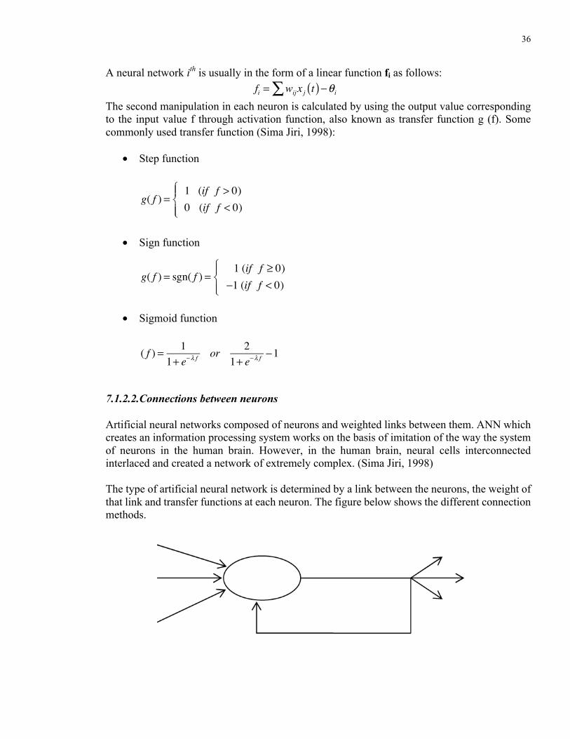
7.1.2.2.Connections between neurons
Artificial neural networks composed of neurons and weighted links between them. ANN which creates an information processing system works on the basis of imitation of the way the system of neurons in the human brain. However, in the human brain, neural cells interconnected interlaced and created a network of extremely complex. (Sima Jiri, 1998)
The type of artificial neural network is determined by a link between the neurons, the weight of that link and transfer functions at each neuron. The figure below shows the different connection methods.
fi = wijx j t( )−θi∑
g( f ) =1 (if f > 0)0 (if f < 0)
⎧⎨⎪
⎩⎪
g( f ) = sgn( f ) = 1 (if f ≥ 0)−1 (if f < 0)
⎧⎨⎪
⎩⎪
( f ) = 11+ e−λ f
or 21+ e−λ f
−1

37
FIGURE 14. Neural Networks with only one node and one feedback connection (Sima Jiri, 1998)
FIGURE 15. Single layer feed-forward network (Sima Jiri, 1998)
Single layer feed-forward neural network is a type of network that only consists of a single layer of output nodes; the inputs are fed directly to the outputs via a series of weights. This type of network is also called single layer perceptron network. Each output neuron can receive signals from the inputs x1, x2, ..., xm to create a corresponding output signal.
FIGURE 16. Multi-layer feed-forward network (Sima Jiri, 1998)

38
In the multi-layer feed-forward neural network, input layers does not convert information but instead, only receives signals. Output signal is given from the output layer. The layer in the middle of input and output layer is called hidden layer. In feed-forward networks, there is no node that has its output as an input of another node on the same layer or layers prior to it. Feedback network is the output of a network that neurons can become the input of the neurons in the same layer or the previous layer. A network that has closed-cycle feedback is called regression network (recurrent network).
FIGURE 17. Single layer recurrent network (Sima Jiri, 1998)
7.1.2.3.Learning in a Neural Networks As mentioned at the beginning, learning process is one of three important factors that make up an artificial neural network. There are two issues to be learned for each artificial neural network, that is parameter learning and structure learning. (Sima Jiri, 1998) Parameter learning is the change of weights of connections between neurons in a network, while structure learning is the adjustment of the structure of the network including changing the number of layers of neurons, the neurons of each layer and the link between them. These two problems can be performed simultaneously or separately. (Sima Jiri, 1998) In terms of learning methods, it can be divided into three categories: supervised learning, reinforcement learning, and unsupervised learning.
7.1.3. Applicability of Artificial Neural Network
The characteristic of artificial neural network is that it is capable of learning and parallel processing. It can approximate the relationship between the complex correlation inputs and outputs of the process which needs to be studied and once it learned, the independent test often

39
gives good results. After completing the studies, artificial neural network can calculate outputs corresponding to the input of new data. (Sima Jiri, 1998) Structurally, artificial neural network is a system composed of many simple processing elements operating in parallel. This feature of ANN allows it to be able to solve large problems. In terms of mathematics, according to Kolmogorov's theorem, a random continuous function f (x1, x2, .., xn) defined on the interval In (with I = [0,1]) can be expressed as :
including: χj, Ψij is continuous functions of one variable. Ψij is monotonic function, regardless of the function f. On the other hand, the model of artificial neural network allows links weighted nonlinear elements (individual neurons) to create synthetic forms of content from the content component. Thus, after a process of adjusting the appropriate link (the learning process), the non-linear element that will make up a complex nonlinear function capable of performing the function approximation process should be studied. As a result, its output will be similar to the output of the data set used to train the network. Besides, it is said that the neural network has learned the correlation relationship of input - output of the process and save this important relationship through the link weights between neurons. Therefore, the artificial neural network can compute on new input data set to produce the corresponding outputs. (Sima Jiri, 1998)
Linear Regression
Approximation using Neural Networks
FIGURE 18. The difference between Linear Regression and Neural Networks Regression. (Sima Jiri, 1998)
f (x) = χ j ψ ij (xi )i=1
n
∑⎛⎝⎜⎞⎠⎟j=1
2n+1
∑
Y = a1x + a2 Y = f x,a1,a2,...,an( )

40
With those characteristics, artificial neural networks have been used to solve many problems in many areas of the different sectors. The application group that artificial neural network has been applied very effectively are: • Classification problem: this type of problem requires solving problems sorting objects into
groups observed based on the characteristics of the groups that object. This is a base problem of many problems in practice: handwriting recognition, voice, genetic classification, classification of product quality, etc.
• Forecasting problem: artificial neural networks have been successfully applied in the construction of predictive models using data sets in the past to predict future data. This is a difficult problem and the group is very important in many branches of science.
• Control and optimization problem: Thanks to the ability to learn and function
approximation that artificial neural network has been used in many automatic control system as well as contributing to solving the optimization problem in practice.
In short, the artificial neural network is considered as a promising approach to solve the nonlinear and complex problem.
7.2. Feed-forward Neural Networks
7.2.1. Single-layer Perceptron Neural Networks
Single-layer perceptron network proposed by F.Rosenblatt 1960 is only a single-layer feed-forward networks in and out without a hidden layer. Each layer can have one or more neurons. Neural network models of Rosenblatt use a threshold function which acts as a transfer function. Therefore, should the sum of the input signal be greater than the threshold value, the output value of neuron will be the one, but in the reverse case, it will be 0. (Nikola K. Kasabov, 1998)
Right from the time when Single-layer Perception Network was proposed, it has been used to solve classification problems. An object will be assigned to Class A by neuron i if:
Where w is the weight of the link from neuron j to neuron i, xj is the input from neuron j, and θ is the threshold of neuron i. In the reverse case the object will be assigned to class B.
Outi =1 if neti ≥θ0 if neti <θ
with neti = wijx j is the sum of input from neuron i∑⎧⎨⎪
⎩⎪
wijx j ∑ ≥θ

41
The network-based training supervised learning methods for sample collection study is {(x(k), d(k))}, k = 1,2, ..., p. With d(k) = [d1
(k), d2(k), ..., dn
(k)]T is the output observed corresponding to the input x(k) = [x1
(k), x2(k), ..., xm
(k)]T (where m is the number of inputs, n is the number of outputs, and p the sample pairs input - output used for learning). Thus it is expected that after the learning process, the calculated output y(k) = [y1
(k), y2(k), ..., ym
(k)]T will be equal to the output of the study sample d(k).
FIGURE 19. Single-layer Perceptron Neural Networks. (Nikola K. Kasabov, 1998)
To begin the process of network training, the weights are assigned randomly in the range [-3, 3]. Then adjusting the weights to suit the learning pattern to reduce the error between y(k) and d(k). The implementation steps: • Determine the weighted random. • For each sample form (x(k), d(k)), k= [1, p] perform these steps:
• Calculate the value of y(k) according to formula (4.8) • Identify errors δi in neuron i: δi = di - yi, where di is the output value and yi is the observed
output value calculated at the ith neuron. • Δwij the change in of weight wij (weighted link between input j to neuron i) according to
the formula: Δwij = ηδixj, with η is the speed of learning (0 <η <1).
yi(k ) = g(wi
T xk ) = g wijx j(k )
j=1
m
∑⎛⎝⎜
⎞
⎠⎟= di
(k ) with i= 1,n[ ] & k = 1, p[ ]

42
• Correction wijt+1= wij
t + Δwij = wijt + ηδi
txjt, in which wij
t is the weight after the adjustment at the time t.
Rosenblatt proved that the learning process will converge to network Perceptron the weight W, performed properly study samples on the condition that these patterns indicate discrete points of a linear function separating certain possibilities (f: Rn → R is called a linearly separable function if the set {F-1(xk)}, with xk belonging to the domain of values of f, can separate with each other by the super-flat in the space Rn).
7.2.2. Multi-layer Perceptron Neural Networks
Multilayer perceptron network (MLP) also known as multi-layer feed-forward neural network is an extension of the single perceptron network model with the addition of hidden layers and neurons in the hidden layer transfer content (activation function) nonlinear form. MLP network with a hidden layer is the artificial neural network which is most commonly used. It can approximate the continuous function defined on a limited domain as well as the function is finite set of points sporadic. (Nikola K. Kasabov, 1998) 7.2.2.1.Solve XOR with MLP network
Two lines can be used to separate the case of XOR function. -0,5+x1+x2=0 and -1,5+x1+x2=0 Or in case of 2 inequations:
It can be seen that each equation above can be accomplished by a neuron and the output of these 2 neurons (2 inequations) is the input of an AND function. Therefore, the network can use the following MLP to implement XOR functions of the following functions:
−0,5 + x1 + x2 > 0−1,5 + x1 + x2 < 0
⇔−0,5 + x1 + x2 > 01,5 − x1 − x2 > 0
⎧⎨⎪
⎩⎪
⎧⎨⎪
⎩⎪

43
FIGURE 20. The implementation of XOR function using MLP
7.2.2.2.Back-propagation algorithm Learning algorithm back-propagation method proposed by Rumelhart is one of the most important findings for the development of artificial neural networks. This algorithm is applied to the multi-layer feed-forward neural network in which the neurons can use the transfer function which is the continuous function with different forms. (Nikola K. Kasabov, 1998) The algorithm uses a set of sample of the input pair - to train the network output. For each pair of input - output (x(k), d(k)), back-propagation algorithm makes two following stages: • The first stage, the input sample x(k) are passed from input layer to output layer, and outputs
have been calculated as y(k). • The next phase, an error signal calculated from the difference between the observed output
d(k) to calculate the output y(k) will be transmitted back from the output layer to the previous layer to adjust the weights of the network. For example, we consider the transmission network with a hidden layer below (for larger networks, the operation is similar).
Neural networks are reviewed with m neurons in input layer, l neurons in the hidden layer and n neurons in the output layer. Solid line represents the signal stream is transmitted from input to output while the dashed lines represent the error signal flow is transmitted back from the output.
zq (q=1, …, l)

44
FIGURE 21. Spread signals in the learning process by the method of back-propagation algorithm. (Nikola K. Kasabov, 1998)
We consider a pair of input - output to train network (x, d), for simplicity we remove caps k symbols showing the serial number of the sample in the sample pairs used to train the network. When put to the input x, q secondary neurons in the hidden layer receives signals in the network are:
Neuron q in the hidden layer will calculate and generate results in its output:
Therefore, the input signal of the ith neuron layer will be:
And finally, the output of neuron i in the output layer would be:
This formula says the transmission signal from the input to the output through the hidden layer. Next we consider the error signal is transmitted back from the output layer. First, for each pair of values in – out, a cost function is built as follows:

45
So with a set of p samples, we turn to build such p cost functions. The study of the network's mission algorithm is essentially seeking collective weights W in space RM (M is the number of weights in the network) to turn minimizes the cost function as such. It is worth noting that the minimum shall be conducted consecutively and cyclically for cost functions.
To minimize the cost of such functions, back-propagation algorithm uses reduced gradient method to adjust the weights connections between neurons. The essence of this approach is that the error E is drawn as a function of the parameter caused the error will have the minimum at the given value of the parameter. When observing the slope of the curve, we will decide to change the parameter to how close to the minimum needed more searches. In the figure below, the value of the weight must be reduced if the derivative dE/dW is positive:
FIGURE 22. Error E is considered as a function of the weight W (Nikola K. Kasabov, 1998)
By the expression, we can perform the reduced gradient method as follows:
With η is a positive constant determines the speed decreases the value of w, and negative sign indicates dimensional gradient reduction. Apply reduced gradient method for weighting links between neurons in the hidden layer to the output layer of neurons, we have:

46
As the error function E is a complex function and the indirect function of the weighted wiq (formula 4.13). Using the principle of taking the derivative of the indirect function !"
!#, we have:
δoi is the wrong signal and index oi means the ith node in the output layer. The error signal is calculated as follows:
In the formula above, neti is the ith neuron in the output layer and g'(neti) = ∂g(neti) / ∂net. Similar results applied to delta learning rule of single perceptron network with input layer is now ZQ output of hidden layers. To adjust the weight of the link between the input layer and the hidden layer, we also use reduced gradient method and taking derivative intermediate variables as above apply. Considering the links between neurons j in the input layer and the qth neuron in the output layer:
From formula 4.13, each component error [di-yi], i = 1, 2, ..., n, is a function of the formula ZQ. Therefore, the formula above can continue to change:
According to the formula 4.13, the formula 4.15 can be rewritten as:
With δhq is the error signal of neuron q in the hidden layer and is defined as follows:

47
With netq is the input of neuron q, the error signal of neurons in the hidden layer is different from the error in the output layer (according to formulas 5.17 and 5.21). Because of this difference, the weight adjustment procedure called expanded delta learning rule. Looking back on the formula (5.21) of the error signal δhq of neuron q in the hidden layer, δhq is determined from the δoi error signal of the neurons in the output layer. Generally, back-propagation law has the form:
In which "output_i" is the output of neuron i and "input_j" is the input of neuron j, signal δi is defined in formula 4.10. From the analysis above, back-propagation algorithm was constructed as follows: Considering a feed-forward neural network with Q class, q = 1, 2, ..., Q, and called neti and yi is the input and output of the ith neuron in the class q. This network has m inputs and n outputs. Let qwij be the weight of the link of the jth neuron in layer q-1 to the ith neuron in layer q. Input: A set of learning sample pairs {(x(k), d(k)) | k = 1, 2, ..., p} and the input vector is supplemented with x(k)
m+1=-1. Step 0 (initialization) Choose a constant η> 0 and Emax (tolerance). Randomly initialized weights in the range of small value. Put E = 0 and k = 1. Step 1 (implement an iterative process for network training) Use kth learning samples: In class on (q = 1), for all i we have: qyi = 1yi = x(k)
i Step 2 (spreading signal from input layer to output layer)
Step 3 (Determining the error signal Qδi at the output layer)
Step 4 (Back-propagation) Back-propagation is to adjust the weights and calculates the error signal q-1δi for classes in advance:

48
• and
• with q = Q, Q-1, …, 2
Step 5 (Test loop condition) Check: If (k<p) then
Begin k = k + 1; Goto Step 1;
End Else
Goto Step 6;
Step 6 (Check whether the total current error is accepted) If (E < Emax) then
{end the learning process and give the last weights} Else
Begin E=0; K=1; Goto Step 1 {start the next learning process};
End; Every time when the entire training set is spread over a network, it is called an epoch. Epoch number depends on the specific case and the initial launch. In some cases, the algorithm must execute tens of thousands of new epoch to converge a solution. The initialization parameter mismatch can cause the learning process to not achieve satisfactory results. With each epoch, the average error of the network is calculated according to the following formula:

49
In which p is the number of samples used to train the network, n is the number of variables of the output vector. RMS error is often used to evaluate the results of the neural network learning. 7.2.2.3. Several factors affect the learning process by the method of error propagation
1. Initialize the weights
The initialization values for the initial weights in the back-propagation network greatly affect the final results of the network. These values are usually randomly initialized within a relatively small value. Typically, transfer function used for network is sigmoid MLP, so if we choose the initialization values with greater weight then these functions can be saturated from the beginning and can lead to clogged systems at one pole local cottage or in a flat area that is close to the starting point. According to a research by Wessels and Barnard, 1992, the initialization of links wij should be in range [−3/ 𝑘);3/ 𝑘)] with ki is the number of links of neuron j to neuron i. (L.Wessels, E.Barnard, 1992)
2. Constant learning η
Constant learning η is also a key factor affecting the effectiveness and convergence of back-propagation algorithm. No constant η is suitable for all the different problems. Constant learning is usually chosen empirically for each specific application problems by trial and error method. (L.Wessels, E.Barnard, 1992) Many practical applications showed that a constant learning can fit at the start of the learning process but it is inconsistent with a later stage of the learning process. Therefore, there is a more effective method which is to use an adaptive learning constant. A simple way to handle this problem is to check whether the weights are reducing prices or not functioning, if not, the weights could probably go far beyond the minimum areas and so constant η needs to reduce. Conversely, if after a few loops, cost functions decreased consecutively, then we can try to increase constant η to speed up the speed of convergence to the minimum value. In 1991, the Hertz and his research colleagues have proposed the law governing constant η as follows: (L.Wessels, E.Barnard, 1992)
With ΔE is the change in cost functions, a and b are positive constants. Whether ΔE is considered always smaller than 0 or not depends on the evaluation of k successive iterations.
3. Constant inertia
Δ =+a if ΔE always < 0 (continuous decrease of the cost function)−bη if ΔE > 0 0 other cases
⎧
⎨⎪
⎩⎪

50
The speed of learning back-propagation algorithm can be very slow if the constant is small, but if the constant is big, it could cause greater fluctuations in the process of finding the minimum value in the reduced gradient method. To solve this problem, it is common to add components to the equation inertia weights adjusted as follows: (L.Wessels, E.Barnard, 1992)
with α is constant inertia, α ∈ [ 0, 1]
Thanks to this component, the learning process can overcome local minimum points to reach a global minimum point. Besides, inertia components also prevent the abrupt change of the weights in the other direction to the direction in which solutions are moving to.
FIGURE 23. Inertia in reality
4. Cost function
In this study, the cost function is selected as a function squared error 𝐸 𝑤 = /0
(𝑑) − 𝑦))05)6/ .
However, it can be replaced by a function F(yi, di) which has derivatives and reaches minimum when the 2 arguments di, yi are equal. Normally the form of a cost function is: (L.Wessels, E.Barnard, 1992)
𝐸 𝑤 = /7
(𝑑) − 𝑦))75)6/ with 1 ≤ p ≤ ∝
7.3. Some issues to consider when using MLP networks
Multi-layer perceptron neural network is a type of neural network used in many practical applications. However, in order to enable the network to give good results, we need to consider a number of issues that have important impacts on the efficiency including: - Standardization of input data - Under fitting and over fitting in learning process of the network - The problem of choosing a suitable network structure
7.3.1. Standardization of input data
MLP network is often used sigmoid transfer function which has the following form:

51
FIGURE 24. Sigmoid function g(x) = 1/(1+e-x)
With this functional form, the output value of each neuron is within the range (0,1), and it reached saturation values (approximately 0 or 1) when ⎢x ⎢is large. Therefore, when the input of the network has a large absolute value, we need to standardize it for some small value, otherwise the neurons in the original hidden layer could immediately reach saturation and learning process of the network can not reach a desired result. Its functional form as on the input value of the network is usually standardized on about in the interval [-3, 3]. On the other hand, due to the output signal of the neurons in the range of values (0.1), the actual output values in the form of standardization should also learn about the value of this to be used for the process of network training. Therefore, in the calculation process, to have the actual value at the output of the network we need to transfer the values in the range of (0.1) in the domain of the actual value. (R. Caruana, S. Lawrence, Lee Giles. 2000)
7.3.2. Under fitting and over fitting in learning process of the network
The key issue when constructing an artificial neural network is how the network is capable of high generalization to give good results even in the cases where the input of the network is not in the sample set used to train. Like other non-linear regression models, we also have to solve two problems: under-fitting and over-fitting in the learning process. When the network structure (number of hidden nodes and links) as well as the number of training times are not enough compared to the needs of the problem, it will disable the network to described approximate correlation relationship between input and the output of the process to forecast and lead to insufficient training. Conversely, if the network is too complex (too many nodes and too many hidden parameters) and learn "too close" to the sample used to train the network, it can lead the network to eventually learn noise components in the sample. This situation is thus called the over-fitting issue of the network. The issue above can cause many kinds of neural networks, especially networks MLP to predict false results compare to reality. (R. Caruana, S. Lawrence, Lee Giles. 2000) Some solutions for learning processes: • Using good representative data to train the network:

52
This is considered a good way to avoid over-fitting. When the network training sample set is used to express multiple possible states of the process, the network will have the ability to generalize relatively well from that data set and will not be affected by over-fitting phenomenon. Also, following measures can significantly helps overcome the over-fitting of the network. (R. Caruana, S. Lawrence, Lee Giles. 2000) • Selecting an appropriate model structure:
The choice of the network model (the hidden layer, the neurons on each hidden layer) has an important influence on the phenomenon under-fitting and over-fitting network. Steve Lawrence's research and C.Lee Giles on interpolation function y = sin(x/3) + v, 0 ≤ x ≤ 20. When v is a random variable with the range (-0.25, 0.25), it can be seen that the network can not learn this function if it is only composed of a hidden node. A network with two nodes is capable of generalizing the best (though not entirely accurate with the sample but it can make a relatively closest shape and it is not too close to the noise of the study sample). The more complex the network (10 hidden nodes, 50 hidden nodes), the more precise it can learn, but this would make it too much to learn all noise components, which consequently decreases the generalization and leads to the over-fitting phenomenon. (R. Caruana, S. Lawrence, Lee Giles. 2000)
FIGURE 25. Top: Polynomial fit to data from y = sin(x/3) + v, 0 ≤ x ≤ 20. Order 20 overfits. Bottom: Small and large MLPs fit to same data. The large MLP does not overfit significantly more than the small MLP. (R. Caruana, S. Lawrence, Lee Giles. 2000)
• Stop learning at the right time:
In 1991, in a study of the learning process of neural network, the authors Nelson and Illingworth found solutions to stop at the right time to avoid over-fitting network learning as follows: (Nelson, M.C. and Illingworth, W.T)
- Divide the sample into two parts: one part is used to train and the other to test. - Use a small initial values.

53
- Use low value of learning rate constant. - Calculate the change of testing error during network training. - Stop studying when testing error begins to see the increases.
7.3.3. Choosing a suitable network size
The work is based on the theorem of Kolmogorov which expected that all continuous mappings from [0,1] p to [0.1] n can be approximated by a three-layer perceptron network layers to include p neurons in the input layer, n neurons in the output layer and (2p+1) neurons in the hidden layer. (Vasco Brattka, 2016) However, it is impossible to figure out the exact number of optimal neural network, the properties of neurons, and specific nonlinear format implemented this approximation. A number of studies on this subject suggested that the optimal number of neurons in the hidden layer is usually smaller than (2p+1). Also, it is necessary to know that the size of learning database must match the network architecture. According to Vapnik and Chervonenkis, the database must have the number of samples:
N ≈ 10. Nw where Nw is the number of network weights. Suppose the number of neurons in hidden layer is L, the number of neurons in the input layer is p, the weights of the connections between input layers and the first hidden layer (including thresholds) is:
D = (p+1). L According to some research results, the number of samples of database needs to satisfy
N ≈ 4.D As the number of database samples have not reached the limit learning, we should reduce the number of connections to avoid rote memorization.
7.4. Combination of Genetic Algorithm and Back-propagation to optimize the
weights in Neural Network
In the previous chapter we have studied the algorithm "back-propagation". This is a learning method of artificial neural network and it allows adjusting the weight of the network to minimize the error function E. This algorithm works on the mechanism of reducing the gradient, with a simple function with extreme gradients, the method helps us to reduce global extreme. However, we know that the error function E in multi-layer neural network is a very complex surfaces

54
function with many local extremes, so this method can not guarantee to find a global extreme price level on the surface. Therefore, to improve the algorithm, it is common to seek to change or add to the constant learning that component to allow inertia to overcome extreme local search process. The choice of constant learning and constant inertia is also a very difficult problem, because if they are too big, it will sometimes lead to instability of the search process, even if they choose too small constant learning and constant inertia to lead to slow learning speed and ability to overcome the local extreme low. The search process on the price as this function has been shown to be a complete NP problem means we can not use a general solution with polynomial complexity to achieve results. (Erik D. Goodman, 2009) Genetic Algorithm (GA) is known as a search algorithm based on the theory of natural selection, and it allows us to achieve global extremes. Dissertation research using genetic algorithms to optimize key problem of artificial neural network can help network learned better. (Erik D. Goodman, 2009)
7.5. Genetic Algorithms
Genetic algorithms have been mentioned in numerous documents, including works by D.E. Goldberg and Thomas Back. This section presents the basic concepts of genetic algorithms as well as its application capabilities. (Erik D. Goodman, 2009) So far, the research and application of information technology have introduced many problems yet to find the method of quick and reasonable solution. Much of that is the optimization problems arising in applications. To solve this problem, it is common to seek an efficient algorithm whose results are only approximate optimal. In many cases we can use probabilistic algorithms, but does not guarantee optimal results, but can choose the error values that will achieve the desired small. (Erik D. Goodman, 2009) According to the probability, the problem is solved in the process of finding space on the set of possible answers. Find the best solution and the process is meant to be optimal. With a small search domain, a number of classical algorithms can be used. However, for large domains, to use artificial intelligence techniques in particular, genetic algorithms are one of those tools. The idea of GA is simulating what nature has done. GA is formed based on the notion that natural evolutionary process is the most perfect, the most reasonable and nature itself optimally. Genetic algorithms applied natural evolution to solve optimization problems in practice (from the set of possible initial solution through evolutionary formation of a new collection with a better solution and will eventually find near optimal solution) (Erik D. Goodman, 2009).
7.5.1. The main idea of a genetic algorithm
Genetic algorithm is a kind of algorithm simulating natural phenomena: inheritance and struggle for survival to improving the survey answers and solution space (Zbigniew Michalewicz, 1992).

55
The concept of inheritance and the struggle for existence is explained through the example of the evolution of a population of rabbits is as follows (Zbigniew Michalewicz, 1992): There is a population of rabbits. Among them, some are more agile and smarter than others. The possibility to be eaten by mink or fox of clever rabbits is smaller than others, so they are surviving and creating more good rabbits. Of course, some sluggish, dull rabbits are still surviving as they were just lucky. The surviving rabbits will start reproducing. The reproduction will create a good mix of "genetic material rabbit": some slow rabbits had children with clever rabbits, some good rabbits with good rabbits, ... And above all, nature occasionally throws in a "wild" rabbit by making genetic material mutant rabbits. The bunny, subsequently will be faster and smarter than the original population because parents are more agile and smarter escaped from mink, fox. (It's good that the fox is also undergoing a similar process, otherwise the rabbits will be quick and smart so that the fox can not catch them). (Zbigniew Michalewicz, 1992) When searching for an optimal solution, the GA also takes steps corresponding to struggle for survival story of rabbits. GA also uses terminology borrowed from genetics. We can talk about the individuals (or genotype, structure) in a population, individuals also known as the chromosome. This can cause a bit of confusion: every cell of an organism of one species has brought some certain types of chromosome (e.g. human has 46 chromosomes), but we are talking about the GA of individuals with a chromosome. The chromosomes are made up of units - the genes - performed in a linear chain. Each gene controls one or more characteristics. Genes with certain characteristics have certain location in the chromosome. Any characteristic of the individual can also manifest itself in a gene that can distinguish and recognize a number of different values. A group of genes (chromosomes) representing a solution of the problem is being solved (meaning, structure of chromosomes can be user-defined). An evolutionary process is performed on a population of chromosomes corresponding to the process of finding a solution in the solution space. (Zbigniew Michalewicz, 1992) Actually, GA belongs to probabilistic algorithms, but is very different from random algorithm because they combine direct search and random search elements. An important difference between the method of GA search and other search methods is that GA maintain and handle a set of solutions (population) while all other methods of handling only find for one point in space. Therefore, GA is much stronger than the existing search methods. The structure of a simple genetic algorithm is similar to the structure of any advanced program. At iteration t, genetic algorithm maintains a population of solutions (chromosomes), 𝑃 𝑡 ={𝑥/=, 𝑥0=, … , 𝑥5= }. Each solution 𝑥)= is evaluated for its "adaptive". Then in the second iteration t+1, a new population is formed by choosing to retain most of the fittest. Some individuals of this population undergo changes thanks to the crossover and the mutation, forming a new solution. Crossover combination allows the properties of the two chromosomes 'father' and 'mother' to create the chromosomes 'child' by permutation of the corresponding gene fragment parents. For example, if parents are represented by 5-dimensional vectors (a1, b1, c1, d1, e1) and (a2, b2, c2, d2, e2), the crossover, permutation in 2nd place will create the child chromosomes (a1, b1, c2, d2, e2) and (a2, b2, c1, d1, e1). Crossover allows the exchange of information between the solutions.

56
Unlike crossover, grafting mutations randomly change one or more genes in the selected chromosome, this change is made with a probability of mutation express speed. Mutation allows adding new information to populations and enriches genetic material.
7.5.2. Diagram of a simple Genetic Algorithm
Genetic algorithm includes the following steps:
1) Initialize the initial population of chromosomes. 2) Determine the value of an objective function for each chromosome. 3) Create a new chromosome by breeding from the current chromosome, taking into
account cross-coupled and mutations occur (if any). 4) Determination of the target for the new chromosome and put it in a new population. 5) If the conditions are satisfied, then stop and return the best chromosome together with
the objective function value of it, if not, return to step 3.
(Brian R. West, Seppo Honkanen. 2005)
Flowchart of the algorithm: (in the next page)

57
FIGURE 26. Flowchart of a simple Genetic Algorithm. (Brian R. West, Seppo Honkanen. 2005)
Initialize the initial population of chromosomes
Determining the value of an objective function for each
chromosome
Create a new chromosome by breeding from the current chromosome, taking into
account cross-coupled and mutations occur (if any).
Determination of the target for the new chromosome and
put it in a new population
If the conditions are satisfied
Stop

58
7.6. Application of genetic algorithms to the optimization problem of the
weight of the artificial neural network
As we all know, using back-propagation algorithm to optimize the weights of artificial neural network is widely used today. However, this algorithm works under the reduced gradient so it is difficult to find global extreme. In this research, genetic algorithm is used to optimize the weight of the network in order to help the learning process better. (Philipp Koehn. 1994) To be able to use genetic algorithm to the study of neural networks, it is necessary to take some steps as follows:
- Construction of cost function - Encoding of chromosomes - Implementation of genetic algorithm
(Philipp Koehn. 1994)
7.6.1. Construction of cost function
The cost function will be used to find the relevance of the individual and of the whole population in the GA. In this study the error function RMSE of the learning sample is used.
RMSE = /75
(𝑦)A − 𝑑)A)05A6/
7)6/
In which:
- yij, dij are the output of the network and the desired output of the output jth in the ith learning sample.
- n is the number of outputs of the network - p is the number of learning samples
In the evolution of the entire population, the cost function will gradually reach a global minimum. (Philipp Koehn. 1994)
7.6.2. Encoding of chromosomes
Each individual in the GA will represent a significant number of neural networks. It is not necessary to distinguish any weight in any layer. It only needs to go all the weights up diagrams of chromosomal genes. (D. Whitley. 1995) a. Binary encoding
A well known chromosome encoding method by Whitley and his co-authors proposal is called GENITOR. There are several versions of GENITOR, basically every major network number is coded into a bit sequence as shown below. Index-bit indicates that the connection exists or not

59
(1 - connected, 0 – not connected). The remaining binary bit string will represent weighted values. Whitley uses 8-bit range from -127 to +127 to encode, 0 is encoded 2 times. With this encoding mutation operators, crossover implementation is quite simple. However, to increase the accuracy, there is a need to increase the number of encoding bits on a weighted encoding. Therefore, the length of the chromosome will increase and this will slow down the execution of the algorithm. (D. Whitley. 1995)
FIGURE 27. Binary encoding of weights using Genitor algorithm.
b. Real number encoding
Montana D. and David L. directly encoded by the weight of real numbers is the value of the weights (D. Montana and L. Davis, 1989). This increases the accuracy of coding as well as reducing the size of the chromosome. In this research we also use this method to perform the encryption of network weights. The gene (weights) are randomly initialized between (-3, +3). However, with this encryption technique we need to change the crossover operator, mutation accordingly. (D. Whitley. 1995)

60
FIGURE 28. Example of real number encoding of weights (D. Whitley. 1995)
7.6.3. Crossover
There are several approaches in crossover chromosomes. (D. Montana and L. Davis, 1989) a. Crossover-weight
Crossover operator will put a value on each position of human chromosomes at random by taking the value at the same chromosomal location of the parent. b. Crossover-nodes
The crossover is performed between nodes and location of the parent. Whenever two nodes in a certain layer are hybridized, the weights of all the incoming links to the node will be permutated.

61
FIGURE 29. Crossover-nodes (D. Montana and L. Davis, 1989)
7.6.4. Mutation
a. Mutate weights
A gene (weights) is randomly selected with a probability of mutation pemutation. There are two methods of mutating weights (D. Montana and L. Davis, 1989):
UNBIASED: each selected gene for mutations will be replaced with a random value around 0.

62
BIASED: each selected gene for mutations will be adding a random value. Montana tested the two methods of this mutate weights. Results showed that BIASED is the better method. This can be explained by considering when executing, a set of weights have a better trend. Therefore, the mutation that replaces the original value with random values around the original value (BIASED) will give better results than the one that is replaced with random values around 0 (unbiased). (D. Montana and L. Davis, 1989)
b. Mutate nodes
Mutation operator will choose the n buttons which are not input buttons. All links to these buttons will be added a random value.
7.7. Combining genetic algorithm and back propagation algorithm to optimize
error weighting artificial neural network
7.7.1. Question
Although Genetic Algorithm is capable of reaching global extreme (minimum and maximum) for the search process, due to the combination of random factors, the search speed is generally very slow. On the other hand, it can not quite reach to the global extreme results that show around it. Opposition to GA, back-propagation algorithm (BP) allows to achieve global extreme if the starting point of the search process is in the global extremes. (Philipp Koehn. 1994)
7.7.2. Combining genetic algorithm and back-propagation algorithm
It is possible to combine the GA and BP to achieve a perfect result of optimization problem weighted in artificial neural network. In this combination algorithm, GA is used as an initialization for BP. Set of weights is coded into the chromosome and is evolved by GA. After the process of evolution, the best weight corresponding to the most elite individuals in the population are chosen as the weight initialization algorithm for BP. It is the set of parameters that allows us to identify the closest point to the maximum point of the cost function. (Philipp Koehn. 1994) With this combination, Back-Propagation algorithm will need to be changed in a few factors: - The algorithm will not generate the weights itself but instead, the weights are received from GA. - Composition of inertia will be removed to increase the speed of the convergence process and eliminate vibrations.

63
7.8. Summary
Firstly, the chapter has given the concept, structure and usability of the artificial neural network. It presented details of multi-layer neural networks feed-forward and learning algorithms for this network type. Artificial neural network is considered to be powerful, flexible to address the problem is nonlinear, complex and particularly in the cases when the relationship between the processes is not easy to setup explicitly. Therefore, its applicability is enormous especially in forecasting problems. However, every algorithm has its own pros and cons. Therefore, in order to optimize the advantages and minimize the disadvantages of the neural network (optimize the weights in the networks), the combination of genetic algorithm and neural network has been selected to use as an improvement for the algorithm. Genetic algorithm is known as a search algorithm based on the doctrine of natural selection, and it allows us to achieve global extremes. Therefore, the application of genetic algorithms on weight optimization in neural network is a potential approach. According to the above analysis as well as the mentioned improvements on methods of mutation which makes the learning process of the neural network better, the combination of the genetic algorithm and back-propagation algorithm should be the main direction for the prediction issue.

64
8. CREATING MATHEMATICAL MODEL OF NEURAL NETWORK
IN THE OPTIMISATION OF THE CASE OF TAXI DISPATCHING.
The first step in the preparation of creating a mathematical model is to create a diagram for a model. Besides, defining input data also enables us to create an actual precise model. After an actual model is created, it is important to have a testing mechanism in order to assess the precision of the model. (WikiHow, 2016) Therefore, this chapter is going to introduce the model diagram, define the input parameters and how can the data be retrieved, as well as give some suggestions about the testing mechanism. However, the creation of actual mathematical model is not mentioned, as the creation is really complex, especially considering the reliability of the model.
8.1. Mathematical Model Diagram
According to the previous chapter, the mathematical model for the optimization of taxi dispatching case is the combination of Neural Network and Genetic Algorithm. Therefore, it is necessary to visualize the diagram of the mathematical model in order to create the next phase of the model. (the diagram is in the next page)

65
FIGURE 30. Diagram of the mathematical model in the optimization of taxi dispatching case.
8.2. Preparation of input data
There are undoubtedly many possible features that can be considered parameters for the model. However, as defined before, the application will be separated into at least 3 parts. The first part will display the possible number of customers in each point, which is arranged in order by distance (this is the most important part, and is predicting by neural network). In each pickup points, users can see the current number of taxis as well as the distance between a given point and the current location (by using Google API, the travel time and total distance can be calculated relatively correct, even if there is a traffic jam). Therefore, by dividing the application into several small tasks, our main task with Neural Network is to predict the possible number of customers in each point based on the given situation. According to the research and the possible parameters from the historical data, the features that need to be taken as parameter in order to train the network are: departure location, departure time, departure date, weather at that moment (temperature, current of air, season in the year, etc).

66
8.2.1. Departure location
Departure location is the location that represent the position of a car when the car starts a new trip. In the database, departure location is saved as the longitude, latitude coordinate, which is pretty handy and precise for the calculation. However, due to the network connection during the transmission of data from the car to the server, or some hardware/software fault of the meter in the car, some data are not confidential, as it could be missing one of the coordinate or even just return null values. Hence, it is essential to have a validation method before using the location data.
8.2.2. Departure date
Departure date is the date when the trip started, it is stored in the database with the time zone set by the setting of the meter.
8.2.3. Departure time
Departure time is the time when the trip started, the time needs to be precise, with detail in seconds.
8.2.4. Climate Features
Climate features are one of the most decisive factor in decision making. In deed, although there are the same departure date, time, and location, there will be a big difference number of consumers for taxi services. Suppose in a sunny day, there are surely more needs for drives than a rainy or snowy day with horrible weather. However, climate features are not the data that were stored in the taxi database. Therefore, a solution for getting this type of data need to be figured out. Fortunately, climate information is important, and also contributing to a lot of modern apps nowadays, for example weather forecast apps, calendar apps, etc. Hence, several public weather info API are offering now. Some can be listed here: (Janet Wagner, PW Staff. 2014)
- Accuweather - Forecast.io - OpenWeatherMap API - Yahoo Weather API - Etc.
All services have their pros and cons, and it is difficult to assess which is better than others. However, considering the popularity and more importantly, with the personal use for some created apps in the past, OpenWeatherMap API is recommended, as they are having fairly simple and good documentation and instruction of how to get the data information with lots of parameters can be passed depend on the users need. Also, current weather, daily forecast, and historical data are accessible by the service. (APPENDIX 5)

67
According to the response, weather type (Clouds, Sunny, …), wind (speed, degree), rain, temperature, humidity will be taken into account.
8.2.5. Events near by / Public holidays
Also like the weather factor, events near by / public holidays can contribute considerably to the consumption of taxicabs services. It is important to collect the events info or the holidays information near by the checking location. For getting all local events happening around a particular location, it is not a simple task. In order to do that, there must be a centralized app that can collect all events information. At the moment, there is no such an absolute sufficient app that can provide this kind of information. Nevertheless, allevents.in service has started to get involve in this business field. And they are getting quite good reputations and feedback for their services at the moment. The idea of the app is that they can provide the upcoming events as well as the whole calendar event (including historical events and future events), which are categorized by the topics such as business, concert, festival, music, sports, parties, exhibitions, meetups, etc. It is worth evaluating the application, and if it is reliable, it can help our application to have a better prediction for the consumption of taxis services. At the moment, allevents.in has just launched the beta version of events API that support developers to get events information from approximately 23000 cities all over the world (including Helsinki) (AllEvent.in, 2016). Below figure can briefly show what the AllEvent.in API can provide us:

68
FIGURE 31. Example of AllEvent.in interface with the request for events in Helsinki in March 2016
Secondly, to get the public holiday information for each countries, the most famous and reliable service provider would be Google Calendar. However, Google is not providing a list of national holidays as a service, it requires a word around method to get that list. Overall, what we can retrieve from them is about the holiday name, date from the country name that was input from the request.
8.2.6. Real collected data
This is the most important and private data, as it was only collected by the association, and not publicly publish anywhere. Therefore, it is essential to have a cooperation with the association in order to start the development process. However, thanks to the help of one of the taxi company, some pieces of data can be presented as bellowed:
FIGURE 32. Sample of statistic data for trips
Another better view can be represented in the below table: TABLE 8. Table of sample of collected data from trips
Shift #
Car Type
Car #
Dep. Date
Dep. Time
Dep. Address
Dest. Address
Cust. #
Dep. Long
Dep. Lat
Dest. Long
Dest. Lat
992 PAL 12 91 3.12.15 11:50 LEPSÄMÄNTIE NUMMIPOLKU 1672 33.75 67.01 33.13 66.75
992 PAL 12 91 3.12.15 09:50 REUNATIE LEPSÄMÄNTIE 441 33.69 66.97 33.75 0
992 PAL 12 91 3.12.15 11:50 LEPSÄMÄNTIE REUNATIE 441 33.75 66.37 33.92 66.93
992 PAL 12 91 3.12.15 09:30 NUMMITIE LEPSÄMÄNTIE 213 33.73 66.97 33.13 66.98
992 PAL 12 91 3.12.15 11:50 LEPSÄMÄNTIE NUMMITIE 213 33.75 66.37 33.75 66.92
6 SAMPO 93 3.12.15 11:30 TÄHTIENTIE MULTATIE 706 0 66.97 33.92 66.98
64 OVELLE 93 3.12.15 15:00 TÄHTIENTIE MULTATIE 1813 33.91 67.01 33.13 66.98
6 SAMPO 93 3.12.15 14:50 HYRYLÄNTIE MULTATIE 414 33.91 66.97 33.75 66.92

69
It can be seen apparently from the highlighted columns that numbers 0 were incorrect or the fields were empty there. Therefore, the validation has to be made before giving the data for the learning process of the algorithm. Besides, not all fields from the data set are helpful for the algorithm of predicting values. In our specific case, the following columns can be considered as the input parameters:
- Departure Date - Departure Time - Departure Address - Departure Longitude - Departure Latitude
The reason why departure address can be used as an input parameter is that in some cases, when the departure longitude/latitude are incorrect, then it is possible to geocode from the actual address to the coordinate format (Google Geocoding API, 2016).
64 OVELLE 93 3.12.15 15:00 TÄHTIENTIE MULTATIE 95 33.91 66.37 33.92 66.98
64 OVELLE 93 3.12.15 08:35 MULTATIE TÄHTIENTIE 1813 0 0 33.13 66.98
6 SAMPO 93 3.12.15 08:35 MULTATIE TÄHTIENTIE 706 0 0 33.75 66.92
64 OVELLE 93 3.12.15 08:35 MULTATIE TÄHTIENTIE 95 25.07 66.97 33.92 66.98
6 SAMPO 93 3.12.15 08:35 MULTATIE HYRYLÄNTIE 414 25.07 66.37 33.13 66.98
6 SAMPO 93 3.12.15 08:35 MULTATIE TÄHTIENTIE 2080 0 0 33.75 66.92
6 SAMPO 93 3.12.15 08:35 MULTATIE TÄHTIENTIE 413 25.07 66.91 33.75 66.98
6 SAMPO 93 3.12.15 08:35 MULTATIE TÄHTIENTIE 1089 0 0 33.13 66.98
6 SAMPO 92 3.12.15 15:00 TÄHTIENTIE YRITTÄJÄNKATU 2822 33.91 66.97 33.75 66.92
6 SAMPO 92 3.12.15 15:00 TÄHTIENTIE YRITTÄJÄNKATU 854 33.91 67.01 33.92 66.98
64 OVELLE 92 3.12.15 15:00 TÄHTIENTIE YRITTÄJÄNKATU 644 33.91 66.97 33.13 66.98
6 SAMPO 92 3.12.15 15:00 TÄHTIENTIE RYPÄLETIE 1169 33.91 66.37 33.75 66.92
6 SAMPO 92 3.12.15 14:50 HYRYLÄNTIE SYDÄNMAANTIE 587 33.91 66.97 33.92 66.98
6 SAMPO 92 3.12.15 14:50 HYRYLÄNTIE SIMEONINTIE 7265 33.91 66.37 33.13 66.91
6 SAMPO 93 3.12.15 08:10 BOSTONINKAARI TÄHTIENTIE 5670 0 0 33.75 0
6 SAMPO 93 3.12.15 11:30 TÄHTIENTIE BOSTONINKAARI 5670 33.91 66.97 33.92 66.93
992 PAL 12 91 3.12.15 09:20 TAKKULANTIE LEPSÄMÄNTIE 229 33.70 67.01 33.13 66.98
992 PAL 12 91 3.12.15 11:50 LEPSÄMÄNTIE TAKKULANTIE 229 33.91 66.97 33.75 66.92
992 PAL 12 91 3.12.15 09:20 SAARIKORVENTIE
LEPSÄMÄNTIE 6017 33.68 66.37 33.92 66.98
992 PAL 12 91 3.12.15 11:50 LEPSÄMÄNTIE SAARIKORVENTIE 6017 33.91 66.91 33.13 66.98
2 TAUKO 93 3.12.15 10:00 726 0 0 33.75 66.92
2 TAUKO 92 3.12.15 10:15 726 0 0 0 66.98
2 TAUKO 97 3.12.15 09:00 726 0 0 0 66.98
6 SAMPO 92 3.12.15 08:05 TEMMONTIE TÄHTIENTIE 7266 0 0 33.92 66.92
…

70
8.3. Indicators to assess the results forecast
The forecast is usually having wrong prediction because the algorithm depends on too many factors including hydrological phenomena as well (weather, etc.), which are complex, difficult to calculate all. To evaluate, compare forecasting methods quantitative way we need to use the index forecast. Here are some of the indicators most commonly used for forecasting: Mean Square Error: (T. Chai, R. R. Draxler. 2014)
(7.1) With:
o : Calculated value at the time of i.
o : Real value at the time of i.
Root Mean Square Error: (T. Chai, R. R. Draxler. 2014)
(7.2)
With:
o : Calculated value at the time of i.
o : Real value at the time of i.
Mean Absolute Error: (Tadd Wood, 2012)
(7.3)
With:
o : Calculated value at the time of i.
o : Real value at the time of i.
Although the index (7.1) - (7.5) are intuitive and easy calculation but in many cases when large data storage or data high volatility, the index becomes too rough. D.R. Legates and G.J. McCabe Jr. presented the indicator E (Coefficient of Efficiency) and indicator r2 (Coefficient of Determination) thought has a higher computational complexity, can overcome the limitations of the indicators though. (P. Krause, D. P. Boyle, and F. Base, 2005)
YiYi
θiθi
fiyi

71
with O observed and P predicted values
Indicators E and r2 can be used in combinations or separately. Good method is a method of getting the value of the major indices. In term of this application, it is suggested that Root Mean Square Error (RMSE) and Coefficient of Determination (r2) should be used in order to assess the accuracy of the forecast.
8.4. Summary
Throughout the chapter, the mathematical model has been visualized, the definition and solution for getting input data has been suggested. Last but not least, the decision of using Root Mean Square Error (RMSE) has also been suggested for building the testing mechanism. Overall, after this step, it is ready to start to create an actual mathematical model of the application according to the lights of previous researches.

72
9. CONCLUSIONS
The thesis did research about the requirement engineering (functional and non-functional requirements), divided the problem of building the application into small sub-problems, gave solutions and orientations to solves each of them. All of the sub-problems are solvable thanks to the existence of API service providers or some simple algorithms except the one that predicts the number of customers at each point at a given time at a given place. In order to solve this most challenging sub-problem, the thesis researched deeply about the possible solutions that can tackle the problem (algorithm selection). Finally, Neural Network is going to be used as not only a modern machine learning technique but also one of the most precise and interesting approach. Chapter 5, 6, and 7 focused on the details of the structure of the Neural Network, the possible combination of Neural Network and Genetic Algorithm, and the input data which need to be provided. The contribution of the thesis
1. Analyze the functionalities of the application in detail, with main mockup interface of how the application works.
2. Consider the non-functional aspects of the application such as the availability, reliability, efficiency, security, and so on.
3. Define the possible system architecture and platform that can be used to build the application.
4. Describe all possible sub-problems and the direction to solve each of them. 5. Select the algorithms that are going to be used to solve the rocket science of the project
– anticipation for the number of customers at each point. 6. Introduce the basic concepts of Artificial Neural Network and Genetic Algorithm. 7. Introduce the research methods of genetic algorithm combined with the back-
propagation algorithm to achieve a perfect result for the optimization of the weight in artificial neural network.
8. Introduce the assessment methods that can be used to check the error of the prediction.
Further development After the thesis, the problem seems to be significantly less complicated than the first approach. However, there are still a lot of improvements that can be done through the application. For example, at the beginning, the application only suggests the possible number of customers at each searching point, but for further development, according to the historical incomes, the predicted income for the trip can also be included as a feature. Besides, the selected algorithm is not the only way that can solve the problem. Indeed, in terms of machine learning technique, one may ask a question that whether Support Vector Machine (SVM), Decision Tree, etc. can also be used to solve the prediction? There have been many studies worldwide that have successfully used this method in the problem of time-series forecasting. Hence, one of the

73
subsequent developments of the research is to study, improve and test the methods for advanced machine learning that can improve forecasting results and forecast period. However, it is realized that, the input data set greatly affect the completeness of forecasted results. Also, some of the input parameters such as weather information and traffic suggestion are also the predicted information, and their accuracies will greatly affect the accuracy of the whole application. Therefore, it is essential to have both reliable API service providers and a good error checking mechanism. Besides, accompanied with the development, it is worthwhile to put effort on collecting good historical data in order to test and evaluate the forecast results.

74
10. REFERENCES
Elizabeth Hull, Ken Jackson and Jeremy Dick. 2005. Requirements Engineering. United States of America: Springer. Lawrence Chung, The University of Texas at Dallas. 2015. Non-functional Requirements. Available: https://www.utdallas.edu/~chung/SYSM6309/NFR-18-4-on-1.pdf Accessed 22 December 2015. Roxanne Miller. 2008. What is the difference between functional and nonfunctional requirements? Why do I need both? Available: http://searchsoftwarequality.techtarget.com/answer/Functional-and-nonfunctional-requirements Accessed 21 December 2015. Matthew Baxter-Reynolds. 2011. Apple's Siri voice recognition: sounds like Tomorrow's World today. Available: http://www.theguardian.com/technology/blog/2011/oct/10/apple-siri-voice-recognition Salesforce UK. 2015. Why move to the cloud? 10 Benefits of cloud computing. Available: https://www.salesforce.com/uk/blog/2015/11/why-move-to-the-cloud-10-benefits-of-cloud-computing.html Accessed 10 January 2016. Jakob Niesel. 2009. Response Times: The 3 Important Limits. Available: https://www.nngroup.com/articles/powers-of-10-time-scales-in-ux/ Accessed 11 January 2016. Jakob Niesel. 2009. Powers of 10: Time Scales in User Experience. Available: https://www.nngroup.com/articles/powers-of-10-time-scales-in-ux/ Accessed 11 January 2016. Jan Stafford. 2011. Improving software performance: Mobile, cloud computing demand APM. Available: http://searchsoftwarequality.techtarget.com/tip/Improving-software-performance-Mobile-cloud-computing-demand-APM Accessed 11 January 2016. Turkka Keinonen. Usability of Interactive Products. UIAH publication A21. Helsinki 1998. Available: http://www2.uiah.fi/projects/metodi/158.htm Accessed 12 January 2016. Bev Littlewood, Lorenzo Strigini. 2014. Software Reliability and Dependability: a Roadmap. Available: http://www.cs.ccsu.edu/~stan/classes/CS530/Notes14/11-DependabilityAndSecurity.html

75
Accessed 15 January 2016. Sommerville, Software Engineering, 9 ed., Chapters 11 & 12. Available: http://www.cs.ccsu.edu/~stan/classes/CS530/Notes14/11-DependabilityAndSecurity.html Accessed 16 January 2016. Scottge. 2015. How to Choose a Machine Learning Algorithm for Regression Problems. Available: http://scottge.net/2015/07/03/ml101-how-to-choose-a-machine-learning-algorithm-for-regression-problems/ Accessed 20 January 2016. Hemant Ishwaran and J. Sunil Rao. 2009. Decision Tree: Introduction. Available: http://treeplan.com/chapters/introduction-to-decision-trees.pdf Accessed 22 January 2016. Simon Haykin. 2009. Neural Networks and Learning Machines. Third Edition. Hamilton, Ontario, Canada. McMaster University. Sima Jiri, 1998. Introduction to Neural Networks, Technical Report No. V 755, Institute of Computer Science, Academy of Sciences of the Czech Republic. Lekkas DFD of C. ONOF .2005. Improved flow forecasting using artificial neural networks, 9th International Conference on Environmental and Technology, Rhodes Island, Greece. Available: http://www.srcosmos.gr/srcosmos/showpub.aspx?aa=6642 Accessed 25 January 2016. Bogdan OAncea, Stefan Cristian Ciucu. 2013. Time series forecasting using neural networks. Available: http://arxiv.org/pdf/1401.1333.pdf Accessed 26 January 2016. Nikola K. Kasabov. 1998. Foundations of Neural Networks, Fuzzy Systems, and Knowledge Engineering. Available: http://boente.eti.br/fuzzy/ebook-fuzzy-kazabov.pdf Accessed 27 January 2016. L. Wessels, E. Barnard. 1992. Avoiding False Local Minima by Proper Initialization of Connections, IEEE Trans. on Neural Networks. Available: https://www.researchgate.net/publication/3301678_Avoiding_false_local_minima_by_proper_initialization_of_connections Accessed 31 January 2016. R. Caruana, S. Lawrence, Lee Giles. 2000. Over-fitting in Neural Nets: Back-propagation, Conjugate Gradient, and Early Stopping. Available: http://papers.nips.cc/paper/1895-overfitting-in-neural-nets-backpropagation-conjugate-gradient-and-early-stopping.pdf

76
Accessed 3 February 2016. Nelson, M.C. and Illingworth, W.T. 1991. A Practical Guide to Neural Nets, Reading, MA: Addison-Wesley. Vasco Brattka. A Computable Kolmogorov Superposition Theorem. Available: http://cca-net.de/vasco/publications/kolmogorov.pdf Accessed 5 February 2016. Erik D. Goodman. 2009. Introduction to Genetic Algorithms. Available: http://www.egr.msu.edu/~goodman/GECSummitIntroToGA_Tutorial-goodman.pdf Accessed 7 February 2016. Thomas Bäck. 1996. Evolutionary Algorithm in Theory and Practice, Oxford University Press. D. Whitley. 1995. Genetic Algorithms and Neural Networks. Available: http://citeseerx.ist.psu.edu/viewdoc/download?doi=10.1.1.18.2120&rep=rep1&type=pdf Accessed 11 February 2016. Zbigniew Michalewicz. 1992. Genetic Algorithms + Data Structures = Evolution Programs. Available: http://web.ist.utl.pt/adriano.simoes/tese/referencias/Michalewicz%20Z.%20Genetic%20Algorithms%20+%20Data%20Structures%20=%20Evolution%20Programs%20(3ed).PDF Accessed 11 February 2016. Brian R. West, Seppo Honkanen. 2005. Determination of ion exchange parameters by a genetic algorithm. Available: http://opticalengineering.spiedigitallibrary.org/article.aspx?articleid=1101644 Accessed 11 February 2016. D. Whitley, T. Starkweather, and C. Bogart, "Genetic Algorithms and Neural Networks: Optimizing Connections and Connectivity," Parallel Computing, 14 (1990) 347-361. Wen-Cheng Liu, Chuan-En Chung. 2014.Enhancing the Predicting Accuracy of the Water Stage Using a Physical-Based Model and an Artificial Neural Network-Genetic Algorithm in a River System. Available: http://www.mdpi.com/2073-4441/6/6/1642/htm Accessed 11 February 2016. Philipp Koehn. 1994. Combining Genetic Algorithms and Neural Networks: The Encoding Problem. Available: http://homepages.inf.ed.ac.uk/pkoehn/publications/gann94.pdf Accessed 11 February 2016. D. Montana and L. Davis. 1989. Training feed-forward neural networks using genetic algorithms. In Proceedings of the Eleventh International Joint Conference on Artificial

77
Intelligence, 762-767, Morgan Kaufmann, San Mateo, CA. Available: http://www.ijcai.org/Proceedings/89-1/Papers/122.pdf Accessed 14 February 2016. T. Chai, R. R. Draxler. 2014. Root mean square error (RMSE) or mean absolute error (MAE)? – Arguments against avoiding RMSE in the literature. Available: http://www.geosci-model-dev.net/7/1247/2014/gmd-7-1247-2014.pdf Accessed: 14 February 2016. Tadd Wood. 2012.Using Mean Absolute Error for Forecast Accuracy. Available: http://canworksmart.com/using-mean-absolute-error-forecast-accuracy/ Accessed: 14 February 2016. WikiHow. 2016. Preparing to Make a Mathematical Model. Available: http://www.wikihow.com/Make-a-Mathematical-Model Accessed 14 February 2016. TaksiHelisnki - Taxi Stands. 2016. Available: http://www.taksihelsinki.fi/en/taxi-stands Accessed 5 February 2016. Google Maps Distance Matrix API. 2016. Available: https://developers.google.com/maps/documentation/distance-matrix/intro#RequestParameters Accessed 10 February 2016. Paul Suarez. 2016. Google Quietly Pulls Flawed Travel Times from Maps. Available:http://www.pcworld.com/article/235898/google_quietly_pulls_flawed_travel_times_from_maps.html Accessed 12 February 2016. Janet Wagner, PW Staff. 2014. Top 10 Weather APIs. Available: http://www.programmableweb.com/news/top-10-weather-apis/analysis/2014/11/13 Accessed 18 February 2016. Xavier Amatriain, Justin Basilico. 27 March 2013. Available: http://techblog.netflix.com/2013/03/system-architectures-for.html Accessed 11 April 2016. Open Weather Map. 2016. Weather API. Available: http://openweathermap.org/api Accessed 20 February 2016. AllEvent.in. 2016. All Event API. Available: http://allevents.in/pages/api Accessed 22 February 2016.

78
Google Calendar API. 2016. Available: https://developers.google.com/google-apps/calendar/overview#apis_explorer Accessed 25 February 2016. Google Geocoding API. 2016. Available: https://developers.google.com/maps/documentation/geocoding/intro#Geocoding Accessed 28 February 2016. P. Krause, D. P. Boyle, and F. Base. 2005. Comparison of different efficiency criteria for hydrological model assessment. Available: http://www.adv-geosci.net/5/89/2005/adgeo-5-89-2005.pdf Accessed 1 March 2016. Use Case UML diagrams 2015. UML Use Case Diagrams: Guidelines. Available: https://msdn.microsoft.com/en-us/library/dd409432.aspx Accessed 21 March 2016. IDC. 2015. Smartphone OS Market Share, 2015 Q2. Available: http://www.idc.com/prodserv/smartphone-os-market-share.jsp Accessed 21 March 2016. Microsoft Azure. 2016. Machine learning algorithm cheat sheet for Microsoft Azure Machine Learning Studio. Available: https://azure.microsoft.com/en-us/documentation/articles/machine-learning-algorithm-cheat-sheet/ Accessed 21 March 2016.

APPENDICES
APPENDIX 1
TABLE 9. User Login
Use case ID UC 2
Use case name Login to the application
Actors Taxi Administrator, Driver, Application DB
Description
1. User login to the system
2. The login credentials is authorized by sending to Application DB
3. Application DB confirms the credentials
4. User is redirected to the main screen
Trigger Taxi Administrator, Driver
Pre-conditions Application downloaded or the website is accessed Normal Flow User input username and password in the login form Alternative
Flows None.
Exceptions If someone tries to login more than 5 times, the system will disable the login process in 1 minute. Reset password or request for a new password is also a possibility.
Post conditions Users will get an error message if the username/password is incorrect, or will be authenticated by the system.
TABLE 10. User setting
Use case ID UC 4
Use case name Edit user settings
Actors Taxi Administrator, Driver, Application DB
Description User can change the personal information (username, password, phone,
email, address, etc.)
Trigger Taxi Administrator, Driver

Pre-conditions Authorized user
Normal Flow Users go to the setting page, and change their basic information (phone number, email address, name, date of birth, address) or update new username/password.
Alternative
Flows None.
Exceptions None. Post conditions Setting data updated.
TABLE 11. Select Language
Use case ID UC 5
Use case name Select Language
Actors Taxi Administrator, Driver, Application DB
Description User can select the preferred language
Trigger Taxi Administrator, Driver
Pre-conditions Authorized user Normal Flow Users go to the setting page, and change the language Alternative
Flows None.
Exceptions None. Post conditions Setting data updated.
TABLE 12. Update username, password
Use case ID UC 6
Use case name Select username, password
Actors Taxi Administrator, Driver, Application DB
Description User can select the username, password
Trigger Taxi Administrator, Driver

Pre-conditions Authorized user Normal Flow Users go to the setting page, and change the username, password Alternative
Flows None.
Exceptions None. Post conditions Setting data updated.
TABLE 13. Voice control system
Use case ID UC 7
Use case name Use Voice dictation
Actors Taxi Administrator, Driver
Description User can access the application features by using the voice control
system
Trigger Taxi Administrator, Drivers
Pre-conditions • Device support voice control, microphone • Authenticated user
Normal Flow User shall be able to dictate the application by using voice control system. For example: request current location, show list of suggestion, etc.
Alternative
Flows None.
Exceptions None. Post conditions The request will be processed by the system.
TABLE 14. Input location
Use case ID UC 9
Use case name Enter input location
Actors Taxi Administrator, Driver
Description User can input the address

Trigger Taxi Administrator, Driver
Pre-conditions Authorized user is finding the suggested stations
Normal Flow Users are finding the suggested stations, and selecting either current location or enter an address.
Alternative
Flows None.
Exceptions None. Post conditions The list of suggestion is displayed.
TABLE 15. Use current location
Use case ID UC 10
Use case name Use current location
Actors Taxi Administrator, Driver
Description User can select use current location
Trigger Taxi Administrator, Driver
Pre-conditions Authorized user is finding the suggested stations
Normal Flow Users are finding the suggested stations, and selecting either current location or enter an address.
Alternative
Flows None.
Exceptions None. Post conditions The list of suggestion is displayed.
TABLE 16. Get direction to go to the selected station
Use case ID UC 11
Use case name Navigator support
Actors Taxi Administrator, Drivers
Description System shall display the anticipated number of customers at each stand in the limited area.
Trigger Taxi Administrator, Drivers

Pre-conditions - Driver has to click one of the suggested stands - Authenticated user
Normal Flow After clicking a suggested location, the application shall redirect the user from main screen to the map that has the navigation system, which is capable of showing the direction for the user.
Alternative
Flows None.
Exceptions None. Post conditions The map is shown to the user.
TABLE 17. Display statistic data
Use case ID UC 12
Use case name Display the statistic data
Actors Taxi Administrator, Drivers, Application DB
Description The application shall display the amount of money that user has accumulated thanks to the suggestion of the app.
Trigger Taxi Administrator, Drivers
Pre-conditions - Driver has to click one of the statistic page - Authenticated user
Normal Flow When user access the statistic feature, the application shall display the amount of money that user has accumulated thanks to the suggestion of the app. In this way, the application shall be able to build the reliability to the users.
Alternative
Flows None.
Exceptions None. Post conditions The map is shown to the user.

APPENDIX 2
- A Google Maps Distance Matrix API request takes the following form:
https://maps.googleapis.com/maps/api/distancematrix/output?parameters
origins=Bobcaygeon+ON|41.43206,-81.38992
destinations=Darling+Harbour+NSW+Australia|24+Sussex+Drive+Ottawa+ON|Capitola+CA
- Latitude/longitude coordinate case:
https://maps.googleapis.com/maps/api/distancematrix/json?units=imperial&origins=40.6655101,-73.89188969999998&destinations=40.6905615%2C-73.9976592&key= YOUR_API_KEY
- Addresses case:
https://maps.googleapis.com/maps/api/distancematrix/json?units=imperial&origins=40.6655101,-73.89188969999998&destinations=enc:_kjwFjtsbMt%60EgnKcqLcaOzkGari%40naPxhVg%7CJjjb%40cqLcaOzkGari%40naPxhV:&key= YOUR_API_KEY

APPENDIX 3 (Google Maps Distance Matrix API, 2016) The Http request below demonstrates a request for the duration and distance to travel between 2 points:
https://maps.googleapis.com/maps/api/distancematrix/json?origins=Vancouver+BC|Seattle&destinations=San+Francisco|Victoria+BC&mode=driving&language=fr-FR&key= YOUR_API_KEY
And here is the JSON format response from the API request:
{ "status": "OK", "origin_addresses": [ "Vancouver, BC, Canada", "Seattle, État de Washington, États-Unis" ], "destination_addresses": [ "San Francisco, Californie, États-Unis", "Victoria, BC, Canada" ], "rows": [ { "elements": [ { "status": "OK", "duration": { "value": 340110, "text": "3 jours 22 heures" }, "distance": { "value": 1734542, "text": "1 735 km" } }, { "status": "OK", "duration": { "value": 24487, "text": "6 heures 48 minutes" }, "distance": { "value": 129324, "text": "129 km" } } ] }, { "elements": [ { "status": "OK", "duration": {

"value": 288834, "text": "3 jours 8 heures" }, "distance": { "value": 1489604, "text": "1 490 km" } }, { "status": "OK", "duration": { "value": 14388, "text": "4 heures 0 minutes" }, "distance": { "value": 135822, "text": "136 km" } } ] } ] }

APPENDIX 5 (Open Weather Map, 2016) The short example is given below illustrate how to get the weather information and how the return data looks: By geographic coordinates
API call:
http://api.openweathermap.org/data/2.5/history/city?lat={lat}&lon={lon}&type=hour&start={start}&end={end}
Example of API response:
{"coord":
{"lon":145.77,"lat":-16.92},
"weather":[{"id":803,"main":"Clouds","description":"broken clouds","icon":"04n"}],
"base":"cmc stations",
"main":{"temp":293.25,"pressure":1019,"humidity":83,"temp_min":289.82,"temp_max":295.37},
"wind":{"speed":5.1,"deg":150},
"clouds":{"all":75},
"rain":{"3h":3},
"dt":1435658272,
"sys":{"type":1,"id":8166,"message":0.0166,"country":"AU","sunrise":1435610796,"sunset":1435650870},
"id":2172797,
"name":"Cairns",
"cod":200}