systemic risk in u.s. crop and revenue insurance programs · systemic risk in u.s. crop and revenue...

Systemic Risk in U.S. Crop and Revenue Insurance Programs

Chuck Mason, Dermot J. Hayes, and Sergio H. Lence

Working Paper 01-WP 266March 2001

Center for Agricultural and Rural DevelopmentIowa State University

Ames, Iowa 50011-1070www.card.iastate.edu

Chuck Mason is senior analyst, Structured Transactions Department, Radian Guaranty, Inc.,Philadelphia. Dermot J. Hayes is Pioneer Hi-Bred Professor of Agribusiness, Department ofEconomics, Iowa State University. Sergio H. Lence is associate professor, Department ofEconomics, Iowa State University.

Journal Paper No. 19232 of the Iowa Agriculture and Home Economics Experiment Station,Ames, Iowa. Project No. IOW03566, and supported by Hatch Act and State of Iowa funds.

This publication is available online on the CARD website: www.card.iastate.edu. Permission isgranted to reproduce this information with appropriate attribution to the authors and the Center forAgricultural and Rural Development, Iowa State University, Ames, Iowa 50011-1070.

For questions or comments about the contents of this paper, please contact Dermot Hayes, 568CHeady Hall, Iowa State University, Ames, Iowa 50011-1070; Ph: 515-294-6185; Fax: 515-294-6336; e-mail: [email protected]

Iowa State University does not discriminate on the basis of race, color, age, religion, national origin, sexualorientation, sex, marital status, disability, or status as a U.S. Vietnam Era Veteran. Any persons havinginquiries concerning this may contact the Director of Affirmative Action, 318 Beardshear Hall, 515-294-7612.

Abstract

The present study estimates the probability density function of the Federal Risk

Management Agency’s (RMA) net income from reinsuring crop insurance for corn,

wheat, and soybeans. Based on 1997 data, it is estimated that there is a 5 percent

probability that RMA will need to reimburse at least $1 billion to insurance companies,

and that the fair value of RMA’s reinsurance services to insurance firms equals $78.7

million. In addition, various hedging strategies are examined for their potential to reduce

RMA’s reinsurance risk. The risk reduction achievable by hedging is appreciable, but use

of derivative contracts alone is clearly no panacea.

SYSTEMIC RISK IN U.S. CROP ANDREVENUE INSURANCE PROGRAMS

Insurance companies have traditionally operated in markets where risk can be pooled

or diversified. Futures and options markets have traditionally operated where risk is

systemic. Yields and revenues obtained by crop producers have both systemic (drought

and price drops) and poolable (localized yield shortfall) risks. Farmers cannot hedge the

poolable or localized source of revenue risk on speculative markets, and insurance

companies will not accept risk that has a systemic component (Gardner and Kramer;

Kramer; Vaughan and Vaughan). As a result, a hybrid mechanism has evolved in U.S.

crop insurance markets wherein the federal government agrees to accept the systemic risk

so that private insurance companies will sell crop and revenue insurance to producers.1

To provide incentives for insurers to offer multi-peril crop insurance, the U.S. gov-

ernment has designed the Standard Reinsurance Agreement (SRA). Under the SRA,

insurers can transfer to the Federal Risk Management Agency (RMA) a portion of losses

that can occur with widespread yield shortfalls, in exchange for ceding their right to a

portion of the gains when premiums are greater than indemnities. The SRA yields an

increasing proportion of the firms’ profits as positive returns increase and commits the

RMA to taking responsibility for an increasing proportion of the losses as they increase.

This leaves the RMA in its role as reinsurer with an uncertain level of total outlays. To

date there has been no attempt to use speculative markets to hedge the systemic portion

of this risk.

The purpose of this study is to break down the total risk absorbed by the U.S. crop

insurance industry into poolable and systemic components. We then use option pricing

theory to value the reinsurance that the federal government provides when it absorbs this

systemic risk. Finally, we evaluate the possibility of using speculative markets in prices

and yields to hedge the systemic risk accepted by the government. The analysis considers

the insurance policies that most contribute to RMA’s risk. These are Actual Production

2 / Mason, Hayes, and Lence

History Buy-Up Coverage (BUP), Actual Production History Catastrophic Coverage

(CAT), the Group Risk Plan (GRP), and Crop Revenue Coverage (CRC).2 The crops

studied are corn, soybeans, and wheat, as they represent the largest of the crops insured

under these programs.

The research presented here is motivated in part by Miranda and Glauber, who argue

that insurance companies could use derivatives markets as substitutes for government

provision of reinsurance. Our work allows the individual insurance companies to pool

their risk under the existing institutional structure and focuses on the systemic risk at a

national level.

Insurance and Reinsurance Programs

Given the focus on RMA’s reinsurance activities, attention is restricted to the major

insurance programs available to farmers that are reinsurable by RMA, i.e., BUP, CAT,

GRP, and CRC.

BUP pays indemnities when a farmer’s yields (y) fall belowψ percent of the average

of the individual’s previous production (Y). In such instances, the farmer gets a payment

per acre insured equal to the yield shortfall multiplied byπ percent of the RMA expected

price (PRMA):

BUP(y; π, ψ) = max[0,π × PRMA × (ψ × Y − y)]. (1)

Farmers can choose price protection levelsπ from the setΠBUP ≡ {0.6, 0.65, ..., 0.95, 1.0}

and yield coverage levelsψ from the setΨBUP ≡ {0.5, 0.65, 0.75}. CAT is similar to

BUP, except that the levels of price and yield protection are fixed at 60 percent and 50

percent, respectively:

CAT(y) = max[0, 0.6× PRMA × (0.5× Y − y)]. (2)

That is, CAT(y) = BUP(y;π = 0.6,ψ = 0.5).

Unlike BUP and CAT policies (whose indemnities are based on the farmers’ indi-

vidual yields), GRP indemnities are based on county yields. Letting Yi and yi

Systemic Risk in U.S. Crop and Revenue Insurance Programs / 3

represent county i’s expected and realized yields, respectively, per-acre indemnities for

GRP are calculated as

GRP(yi; π, ψ) = max[0,π × PRMA × (Yi − yi/ψ)]. (3)

It is clear from (1) and (3) that GRP indemnities are computed differently from BUP and

CAT indemnities, even after accounting for county- rather than farm-level yields. In

particular, the yield coverage level (ψ) under GRP does not define the upper limit of

indemnification, as it does under BUP and CAT. Farmers can select price protection

levelsπ ∈ ΠGRP ≡ {0.9, 0.95, ..., 1.45, 1.5} and yield coverage levelsψ ∈ ΨGRP ≡ {0.7,

0.75, 0.8, 0.85, 0.9}.

CRC is a revenue-protection product and is the most recent of the four programs

analyzed. CRC provides a revenue guarantee equal to the revenue the farmer would get if

his actual yields wereψ percent [ψ ∈ ΨCRC ≡ {0.7, 0.75, 0.8, 0.85}] of the historical

average and the actual price equaled the expected price at planting time. More specifi-

cally, per-acre CRC indemnities can be stated as

CRC(y, Ph; ψ) = max[0, max(Pp, Ph) × ψ × Y − Ph × y], (4)

where Pp and Ph are measures of the planting and harvest prices as defined by the CRC

policy. Price Pp (Ph) is the average daily settlement price during the month prior to planting

(harvest month) of the futures contract month immediately following harvest. From (4), it

is clear that CRC indemnities depend crucially on market prices. This is in sharp contrast

with BUP, CAT, and GRP indemnities, for which market prices are irrelevant.

RMA obligations on the policies written by insurers are determined from the indem-

nity levels described in the SRA. At the insurer’s discretion, each of its written policies

may be ceded to RMA outright (if the policy is sufficiently undesirable) or allocated to one

of three different funds which determine the level of risk transferred to the RMA and the

level maintained by the insurer. In this manner, the insurer may rid itself of its most

undesirable policies and attenuate the risk of the portfolio of policies that it keeps.

In decreasing order of risk, the RMA funds are designated Assigned Risk Fund

(ARF), Development Fund (DF), and Commercial Fund (CF). The high-risk policies that

the insurance company elects to keep are placed in ARF, in which the overwhelming


majority of profits and losses are yielded to the RMA. Due to their high risk for RMA,

for each state there is a limit on the total value of policies that can be placed in ARF. At

the opposite end of the spectrum, insurers will designate as CF only the policies

perceived to pose the least amount of risk to the firm and/or those that stand to yield the

greatest profits.

Simulation Model

Estimating the probability density function (pdf) of RMA’s net income from reinsur-

ance is a complex modeling problem. Schematically, the procedure advocated here

requires first completing the following tasks:

1. Estimating county-level yield pdfs and U.S. level price pdfs that reflect historical

patterns.

2. Calibrating insurance policies and within-county yield pdfs, by using historical

insurance data.

3. Assigning insurance policies to reinsurance funds, based on historical reinsur-

ance data.

Having finished the three tasks above, Monte Carlo simulations are performed to

draw a large number of simulated “annual” observations on crop yields and prices. In

turn, these are used to compute simulated “annual” observations on RMA’s net income

from reinsurance. The histogram of the latter series provides an estimate of the unknown

pdf of RMA’s net income from reinsurance. A more detailed description of the whole

process is provided next.

Simulation of County-Level Yields

Before employing historical yields for estimation purposes, it is imperative to correct

them for the significant productivity advances that occurred over the period analyzed.

The large positive trends in the yields of corn, soybeans, and wheat reported in Table 1

provide strong evidence of the need for such a correction. Table 1 contains estimates of

the regression:


TABLE 1. Ordinary least-squares regression estimates of U.S. yields against time,1972 through 1997

Note: ** denotes significantly different from zero at the 1 percent level based on the two-tailed t-statistic.aVariables with hats ( ) denote sample estimates.bNumbers between parentheses below coefficient estimates are the respective standard deviations.

ln(yUSt) = a0 + a1 t + et, (5)

where yUSt represents U.S. yield in year t, et is an error term, a0 is the intercept, and a1 is

the percentage annual change in yields (source: USDA-NASS). Following Miranda and

Glauber, all of the historical yields used in the remainder of the study consist of 1997-

equivalent yields, obtained by detrending the original yields by means of the percentage

annual yield change estimates shown in Table 1.

Estimation of County-Level Yield pdf’s. Skewness in crop yields has been identified

(e.g., Gallagher; Ramirez) and is particularly important for this study in which insurance

payments result from lower-than-average yields. Although Just and Weninger have raised

concerns regarding the methods used to reject normality in the distribution of yields, the

beta pdf has been used to model the behavior of yields in various studies as a means of

capturing potential skewness (e.g., Nelson and Preckel; Babcock and Hennessy). Here we

adopt the beta pdf (6) because it can reflect various levels of skewness and kurtosis, and

its most appropriate shape can be estimated with historical data rather than imposed in an

ad hoc manner.

B(y| α, β, YL, YU) ≡)()(

)(

βΓαΓβ+αΓ

1LU

1U1L

)YY(

)yY()Yy(−β+α

−β−α

−−−

for YL ≤ y ≤ YU. (6)

Regression Model: ln(yUSt) = a0 + a1 t + et.

Corn Soybeans Wheat

0a a 4.5276** 3.4220** 3.4158**

(0.0268)b (0.0176) (0.0153)

1a 0.01803** 0.01453** 0.00875**

(0.00357) (0.00235) (0.00197)R2 0.430 0.614 0.442Number ofobservations 26 26 26


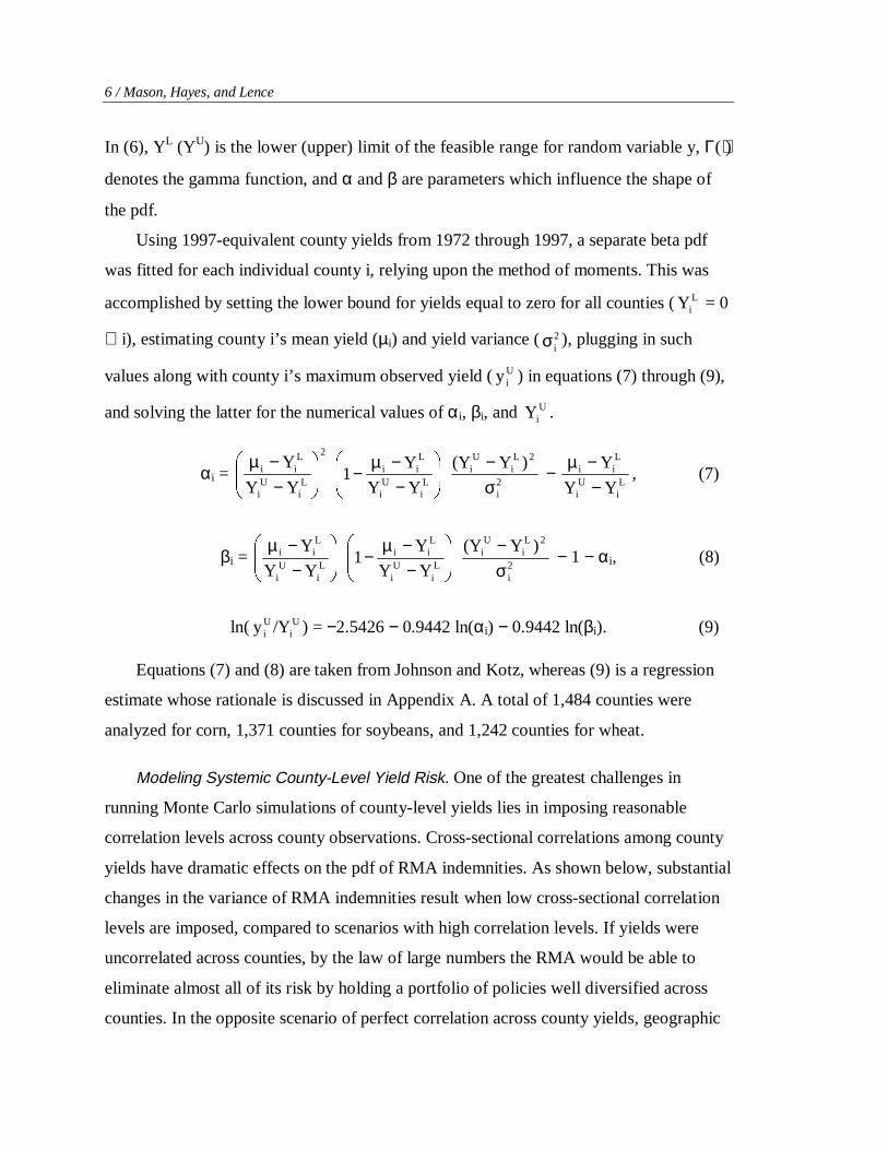
In (6), YL (YU) is the lower (upper) limit of the feasible range for random variable y,Γ(⋅)

denotes the gamma function, andα andβ are parameters which influence the shape of

the pdf.

Using 1997-equivalent county yields from 1972 through 1997, a separate beta pdf

was fitted for each individual county i, relying upon the method of moments. This was

accomplished by setting the lower bound for yields equal to zero for all counties (LiY = 0

∀ i), estimating county i’s mean yield (µi) and yield variance ( 2iσ ), plugging in such

values along with county i’s maximum observed yield (Uiy ) in equations (7) through (9),

and solving the latter for the numerical values ofαi, βi, and UiY .

αi =2

Li

Ui

Lii

YY

Y

−−µ

−−µ

−Li

Ui

Lii

YY

Y1

2i

2Li

Ui )Y(Y

σ− −

Li

Ui

Lii

YY

Y

−−µ

, (7)

βi =

−−µ

Li

Ui

Lii

YY

Y

−−µ

−Li

Ui

Lii

YY

Y1

2i

2Li

Ui )Y(Y

σ− − 1 − αi, (8)

ln( Ui

Ui /Yy ) = −2.5426− 0.9442 ln(αi) − 0.9442 ln(βi). (9)

Equations (7) and (8) are taken from Johnson and Kotz, whereas (9) is a regression

estimate whose rationale is discussed in Appendix A. A total of 1,484 counties were

analyzed for corn, 1,371 counties for soybeans, and 1,242 counties for wheat.

Modeling Systemic County-Level Yield Risk. One of the greatest challenges in

running Monte Carlo simulations of county-level yields lies in imposing reasonable

correlation levels across county observations. Cross-sectional correlations among county

yields have dramatic effects on the pdf of RMA indemnities. As shown below, substantial

changes in the variance of RMA indemnities result when low cross-sectional correlation

levels are imposed, compared to scenarios with high correlation levels. If yields were

uncorrelated across counties, by the law of large numbers the RMA would be able to

eliminate almost all of its risk by holding a portfolio of policies well diversified across

counties. In the opposite scenario of perfect correlation across county yields, geographic


diversification of the policy portfolio would provide no benefits to RMA in terms of risk

reduction. Given that greater geographic correlation of yields reduces diversification

benefits, it is essential for the simulations to maintain an appropriate degree of correlation

among county yield draws.

For analytical and simulation purposes, each state was divided into a small number

of divisions, and each division was divided further into three to five subdivisions

containing a number of counties.Rankcorrelations (McClave and Benson) between

successive levels (e.g., national-state, state-division, and so on) were estimated using

1997-equivalent yield data for 1972 through 1997.3 In general, estimated rank

correlations were very large in high-production areas, and positive but very disperse in

other areas.4 The estimated rank correlations between successive levels of geographic

aggregation were used, along with Johnson and Tenenbein’s method to obtain county-

level yields with the desired cross-correlation structure.

To obtain a single “annual” draw of the set of county yields, first draw one realiza-

tion xUSt for the United States from the uniform pdf with limits of zero and one [U(x)].

Second, draw one realization from U(x) for each state, and use Johnson and Tenenbein’s

approach to convert each of them into a uniform variable with the desired level of

correlation with xUS. Third, draw one realization from U(x) for each division of each

state, and use Johnson and Tenenbein’s technique again to convert each of them into a

uniform variable with the desired level of correlation to the state to which it belongs. This

procedure is repeated at the subdivision and county levels so as to obtain a vector of

county-level variables (xit)—each of them uniformly distributed between zero and one—

that are correlated with each other through their correlations at the county-subdivision,

subdivision-division, division-state, and state-national levels. Finally, convert each of the

uniformly distributed county-level variables xit into a yield realization yit using the

inverse of the corresponding beta pdf, i.e., yit = B−1(xit| αi, βi,LiX , U

iX ). The results

reported in the present study are based on 2,500 “annual” draws. That is, t = 1, ..., 2,500.


Simulation of Harvest Prices

Because the RMA reinsures CRC policies, which guarantee revenues rather than

yields, it is necessary to simulate prices, as well. The price component of the CRC

indemnity (4) is determined by using two price levels (Pp and Ph) in each year. Planting

prices (Pp) are represented by constants equal to the 1997 CRC planting prices, because

the model is calibrated for 1997 and Pp is known at the time of entering the insurance

agreement. Therefore, Pp is set equal to $2.73/bu for corn, $6.97/bu for soybeans, and

$3.99/bu for wheat.

In contrast, harvest prices (Ph) are unknown at the time of signing the insurance

contract. Hence, Ph is treated as a random variable. It is postulated that ln(Ph) is normally

distributed, an assumption commonly made for commodity futures prices (recall that Ph is

a monthly average of futures prices). Data on Ph for 1989 through 1998 were assembled

from RMA Manager’s Bulletins(USDA-RMA) to calculate sample means and variances

of ln(Ph). The estimated parameters are used as parameters for the price pdfs.

The simulated price and yield series mimics the historical correlations between

prices and yields. Correlation coefficients between harvest prices (Pht) and 1997-

equivalent U.S. yields (yUSt) were estimated using (10) with data for years t = 1989

through t = 1998:

UShyPρ =5.01998

1989t

2UStUSt

5.01998

1989t

2ptht

1998

1989tUStUStptht

)Yy(10

1)]ln(P)P[ln(

10

1

)Yy()]ln(P)P[ln(10

1

−

−

−−

∑∑

∑

==

= . (10)

In (10), planting prices (Ppt) are defined as in (4), and YUSt is year t’s expected yields

obtained by applying the regression equation for U.S. yields (5). As predicted by

economic theory, correlation estimates are negative for the three crops, with

UShyPρ = −0.788 for corn,UShyPρ = −0.499 for soybeans, and

UShyPρ = −0.649 for wheat.

The estimated correlations are imposed on the simulated series of harvest prices and

national yields by means of Johnson and Tenenbein’s method. For this particular case,

however, application of Johnson and Tenenbein’s technique requires a trial-and-error

process. The reason for this is that, while simulated observations of (the logarithm of)


harvest prices are obtained directly from the normal pdf, there is no single pdf from

which simulated observations of national yields can be drawn. Instead, each simulated

observation of U.S. yields is obtained by getting one “annual” draw of the vector of

county yields, calculating county-level production figures (by multiplying county yields

by their respective acreages),5 obtaining U.S. output by summing production across

counties, and, finally, dividing U.S. output by total acres.

Calibration of Insurance Policies

Farmers are allowed to choose from a menu of price protection (π), yield coverage

(ψ), and policy premium levels when contracting BUP and GRP, and from a pre-

specified set of yield coverage (ψ) and premium levels for CRC policies. Since actual

data on individual (π, ψ) allocations are not available, a workable method is needed to

proceed with the analysis.6

The method advocated here computescalibratedvalues ofπ andψ for each policy

and each county, and then proceeds as if they were the only price protection and yield

coverage levels available. With calibratedπ andψ values for county i and policy p (p =

BUP, GRP, CRC), county i’s total expected indemnities are equal to total premiums paid

in county i under policy p. That is, calibration yields an expected loss ratio (i.e., total

expected indemnities divided by total premiums paid) equal to one for each county-policy

combination. Because CAT price protection and yield coverage levels are fixed (see [2]),

achieving expected loss ratios equal to one requires a different kind of calibration. As

explained below, CAT calibration is performed by means of the variance of acre-level

yields. Next, we elaborate more fully on these issues.

Total indemnities for policy p in county i and “year” t (Ipit) are calculated using (11):

Ipit = Apit × Ip(yit), (11)

where Apit is the number of acres insured and Ip(yit) is the average indemnity paid per

acre insured. The notation for Ip(yit) stresses that in any given year t, county i’s average

per-acre indemnity paid under policy p crucially depends on the observed county-level

yield (yit).


Because the model is calibrated for 1997, Apit values are taken to be county i’s

number of acres under the corresponding policies in 1997. Formulas for Ip(yit) are policy

specific, the simplest of them being the one corresponding to GRP:

IGRP(yit) ≡ GRP(yit; πGRPi, ψGRPi), (12)

whereπGRPi ∈ (0.9, 1.5) andψGRPi ∈ ΨGRP are county i’scalibratedprice protection and

yield coverage levels for GRP, respectively. Calibration is achieved by selectingπ andψ

so as to equate the expected value of county i’s total GRP indemnities (i.e., AGRPi1997

ΙIGRP(yit) B(yit| αi, βi,L

iY , UiY ) dyit) with county i’s total GRP premiums.7

Formulas for Ip(yit) corresponding to CAT, BUP, and CRC policies are more involved

than (12), as they depend on farm-level yields. For CAT, the formula for Ip(yit) is

ICAT(yit) ≡ ∫ CAT(yait) dΦ(yait| yit,2its ), (13)

where yait is the yield in theath acre of county i in year t, andΦ(⋅| yit,2its ) is the

cumulative normal pdf with mean yit and variance 2its . For numerical tractability, the

integral in (13) is approximated by adding up over ten partitions of the yait range, each

with 10 percent mass probability. All of the yait values within thedth partition are set

equal to ydit ≡ Φ−1(d/11| yit,2its ), whereΦ−1(⋅) is the inverse function ofΦ(⋅).

Acre-level yield means are the simulated state-level yields (yit), because county

yields are simple averages of acre-level yields. Acre-level yield variances (2its ) are

calculated employing (14):

2its = max{0.001, is exp[Φ−1(zit| b30 + b31 xit, b20 + b21 xit)]}, (14)

where is is a county-specific constant obtained bycalibration (see below), zit is a random

number drawn from the uniform pdf U(z), xit is the uniformly distributed county-level

variables used to calculate the state-level yield realization yit (see sub-subsection

“Modeling Systemic County-Level Yield Risk”), and b30, b31, b20, and b21 are a set of

constants whose values are reported in Table B.1. The rationale for the linear equations

involving xit in (14) is discussed in Appendix B.


CAT differs from the other insurance programs in that its price protection and yield

coverage levels are fixed at 0.6 and 0.5, respectively. Hence, the acre-level yield variance

( 2its ) is the only term in (13) that can be calibrated so as to render county i’s CAT

expected loss ratio equal to one.8 Given the variance formula in (14), calibration of2its is

achieved by estimating the constantis .

The expression to compute county i’s average per-acre BUP indemnities in year t is

IBUP(yit) ≡ ∫ BUP(yait; πBUPi, ψBUPi) dΦ(yait| yit,2its ), (15)

whereπBUPi ∈ (0.6, 1.0) andψBUPi ∈ ΨBUP are county i’scalibratedBUP price protection

and yield coverage levels.9 Numerical estimation of (15) is performed following the

same procedure and employing the same (yit,2its ) values that are used to calculate (13).

Finally, average per-acre CRC indemnities are computed from formula (16):

ICRC(yit) ≡ wCRCi ∫ [ ∫ CRC(yait, Pht; ψCRCi) θ(Pht| yUSt) dPht] dΦ(yait| yit,2its )

+ (1 – wCRCi) ∫ [ ∫ CRC(yait, Pht; ψCRCi – 0.05)θ(Pht| yUSt) dPht] dΦ(yait| yit,2its ). (16)

In (16), wCRCi ∈ (0, 1) represents acalibratedCRC acreage share for county i,ψCRCi ∈

ΨCRC is county i’scalibratedCRC yield coverage, andθ(Pht| yUSt) is the conditional pdf

of harvest prices. Analogous to the calibration criterion for all other policies, terms wCRCi

andψCRCi are chosen so as to make county i’s CRC expected loss ratio equal to one. An

interpretation of the linear combination in (16) is that wCRCi percent of acres in county i

are covered at levelψCRCi, and the remaining (100− wCRCi) percent acres are covered at

the immediately lower permitted level.

Allocation to Reinsurance Funds and Simulation of RMA’s Net Income

The final requirement to simulate RMA’s net income from reinsurance activities

consists of allocating policies across reinsurance funds according to the risks they present

to insurers. As pointed out earlier, calibration is achieved by equating expected loss ratios

to one, which is equivalent to setting expected net income from insurance equal to zero.


Despite this, insurance firms can expect to profit from selling insurance because the SRA

is structured so as to provide incentives for them. By judiciously allocating their insurance

policies among RMA’s reinsurance funds, insurance firms expect to extract a positive net

income at the expense of RMA, which must bear the corresponding expected losses.10

The 1997 state-level allocations to each of ARF, DF, and CF in premium dollars are

provided by RMA. In 1997, policies designated CF generally accounted for the largest

dollar amount reinsured by the RMA in the main producing states. For other states,

allocations varied substantially among the three funds. The 1997 state-level allocations

are mimicked in the simulation. This is accomplished by first ranking all of the policies

for a particular state according to their standard deviation of loss ratios (which are

obtained at the calibration stage).11 Then, beginning with the policies with the largest

(smallest) standard deviation, policies are designated ARF (CF) until their share of

premiums reaches the state’s share of premiums designated ARF (CF) in 1997. All

policies yet to be designated are then assigned to DF.12 The process is then repeated for

each of the remaining states.

Having allocated all policies into reinsurance funds, Monte Carlo simulations of

RMA’s net income can finally be performed. Each “annual” observation of RMA’s net

income is obtained by (i) computing total indemnities for each policy and county by

means of (11), (ii ) calculating RMA’s portion of such indemnities and their premiums

according to the reinsurance funds they belong to, and (iii ) adding the figures obtained in

step (2) across counties and policies.

RMA’s Net Income pdfs without Hedging: Results and Discussion

Table 2 contains summary statistics of the RMA’s estimated net income pdfs in the

absence of hedging. For illustrative purposes, the RMA’s estimated net income

cumulative pdfs from reinsuring corn are depicted in Figure 1. To save space, analogous

figures for soybeans and wheat are not included, as they display similar patterns.

Expected net income from reinsuring corn is a loss of $36.3 million, with losses

occurring 40.5 percent of the time. Standard deviation of RMA’s net income for corn is

$295.5 million. Value at risk at the 5 percent and 10 percent levels [VAR(5%) and


TABLE 2. Statistics of the simulated pdf of RMA’s net income without hedging,expressed in millions of dollars

AggregateCorn Soybeans Wheat Hist. Corr.a Perf. Corr. b

Mean −36.3 −24.6 −17.7 −78.7 −78.7Standard

Deviation 295.5 227.7 111.8 473.7 635.0VAR(5%) −633.8 −498.6 −226.2 −1,006.8 −1,358.5VAR(10%) −487.2 −344.3 −171.5 −779.0 −1,003.0Minimum −1,383.8 −1,078.8 −524.9 −2,012.6 −2,987.5Maximum 277.7 221.1 190.8 641.9 689.6

Note: Results are based on 2,500 simulated “annual” observations.a“Hist. Corr.” means simulation results corresponding to historical correlation levels across nationalcrop yields.b“Perf. Corr.” denotes simulation results assuming that yields and prices are perfectly correlated acrossthe three crops.

VAR(10%), respectively] are losses of $633.8 million and $487.2 million, respectively,

and the minimum (maximum) “annual” net income obtained is a $1,383.8 million loss

($277.7 million gain).13

Results for soybeans are similar, albeit on a somewhat smaller scale. Expected net

income is a loss of $24.6 million for RMA in its capacity as reinsurer of soybean policies.

Net income ranges from a loss of $1,078.8 million to a gain of $221.1 million, with losses

observed 42.2 percent of the time. Standard deviation of net income equals $227.7

million. In this instance, VAR(5%) and VAR(10%) consist of losses of $498.6 million

and $344.3 million, respectively.

The scale is smaller still for RMA net income from reinsuring wheat, with an expected

loss of $17.7 million and a standard deviation equal to $111.8 million. The greatest loss

($524.9 million) as well as the largest gain ($190.8 million) for wheat is smaller than the

respective figures for corn and soybeans. In the case of wheat reinsurance, median net

income is a loss, as expenses exceed revenues 50.6 percent of the time. VAR(5%) and

VAR(10%) amount to losses of $226.2 million and $171.5 million, respectively.

For at least two reasons, it is important to estimate the pdf of RMA’s net income

aggregated across crops, as well. First, it may be argued that the ultimate risk faced by

RMA stems from its total potential losses, rather than its potential losses from each

individual crop. Second, it is of interest to assess to what extent diversifying among crops

ameliorates the risk of RMA’s total net income.


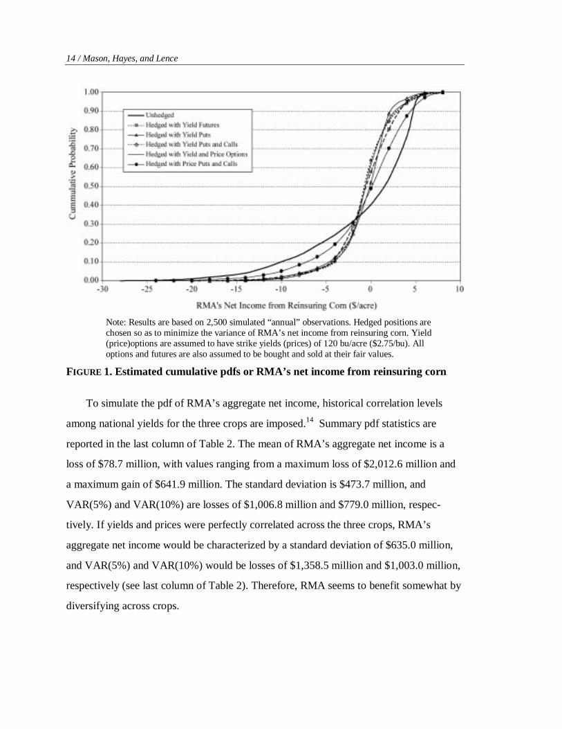
Note: Results are based on 2,500 simulated “annual” observations. Hedged positions arechosen so as to minimize the variance of RMA’s net income from reinsuring corn. Yield(price)options are assumed to have strike yields (prices) of 120 bu/acre ($2.75/bu). Alloptions and futures are also assumed to be bought and sold at their fair values.

FIGURE 1. Estimated cumulative pdfs or RMA’s net income from reinsuring corn

To simulate the pdf of RMA’s aggregate net income, historical correlation levels

among national yields for the three crops are imposed.14 Summary pdf statistics are

reported in the last column of Table 2. The mean of RMA’s aggregate net income is a

loss of $78.7 million, with values ranging from a maximum loss of $2,012.6 million and

a maximum gain of $641.9 million. The standard deviation is $473.7 million, and

VAR(5%) and VAR(10%) are losses of $1,006.8 million and $779.0 million, respec-

tively. If yields and prices were perfectly correlated across the three crops, RMA’s

aggregate net income would be characterized by a standard deviation of $635.0 million,

and VAR(5%) and VAR(10%) would be losses of $1,358.5 million and $1,003.0 million,

respectively (see last column of Table 2). Therefore, RMA seems to benefit somewhat by

diversifying across crops.


RMA’s Net Income pdfs in the Presence of Hedging

The analysis in this section is performed on a per-acre (insured only) basis, to make

it more intuitive. Given the substantial risks stemming from RMA’s reinsurance

activities, it is of interest to investigate the potential to attenuate such risks by hedging

with yield and/or price derivatives. Because the relationship between reinsurance costs

and yields crucially affects the potential for yield derivatives to decrease risks, it is

essential to have simulated observations on national yields in addition to simulated

harvest prices and RMA’s net income. Simulated national yield observations are obtained

as described in the subsection “Simulation of Harvest Prices.”

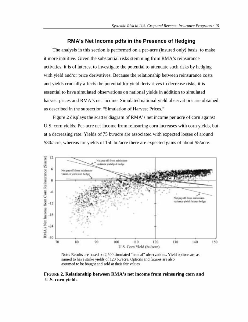
Figure 2 displays the scatter diagram of RMA’s net income per acre of corn against

U.S. corn yields. Per-acre net income from reinsuring corn increases with corn yields, but

at a decreasing rate. Yields of 75 bu/acre are associated with expected losses of around

$30/acre, whereas for yields of 150 bu/acre there are expected gains of about $5/acre.

Note: Results are based on 2,500 simulated “annual” observations. Yield options are as-sumed to have strike yields of 120 bu/acre. Options and futures are alsoassumed to be bought and sold at their fair values.

FIGURE 2. Relationship between RMA’s net income from reinsuring corn andU.S. corn yields


Notwithstanding the strong positive effect of yields on RMA’s net income, there is

substantial variation in net income for any given national yield. RMA may incur losses at

all yield levels, but it may also reap gains, even for yields as low as 90 bu/acre.

The effect of hedging with corn yield futures on RMA’s net income is investigated

first.15 It is assumed that futures contracts are based on planted acres and that RMA

opens its futures position far enough in advance so that yield futures contracts are priced

at their unconditional expected value of 117.6 bu/acre (i.e., the average national corn

yield). It is further assumed that RMA’s hedging objective is to minimize risk, in which

case the optimal hedge is the so-called minimum-variance hedge (e.g., Ederington).

Here, the minimum-variance hedge is a short futures position proportional to the

slope in a regression of RMA’s net income per acre against national yields. The slope

estimate is 0.26, which means that, on average, a one-bushel increase in national yields

increases expected RMA’s net income by $0.26/acre (see Figure 2). Hence, the expected

income of the offsetting yield futures position (i.e., the minimum variance hedge) must be

−$0.26/acre for each unit increment in U.S. corn yields. Adding the income from shorting

the corresponding number of corn yield futures to RMA’s unhedged net income gives

RMA’s net income after hedging.

Simulation results are summarized in Table 3 and illustrated graphically in Figure 1.

Compared to the unhedged scenario, hedging with yield futures leaves RMA’s expected

net income unchanged at−$0.75/acre but substantially reduces the standard deviation of

net income (from $6.11/acre to $3.34/acre). Hedging also reduces the maximum observed

loss from $28.62/acre to $20.64/acre, and increases the maximum observed gain from

$5.74/acre to $8.14/acre. Hedging improves VAR(5%) from a loss of $13.11/acre to a

loss of $6.58/acre, and VAR(10%) from a loss of $10.08/acre to a loss of $4.44/acre.

Given the nonlinear kind of relationship between RMA’s net income and U.S. yields

depicted in Figure 2, holding an appropriate position in corn yield put options should

provide a better hedge than holding yield futures. Yield put payoffs are linear in yields

when yields fall below the puts’ strike yield, so that a put holder’s income increases by a

constant amount per bushel drop in yields under the strike yield. Should final yields be

greater than the yield strike at settlement, the put option expires worthless, limiting the

loss to the amount initially paid to purchase the put.


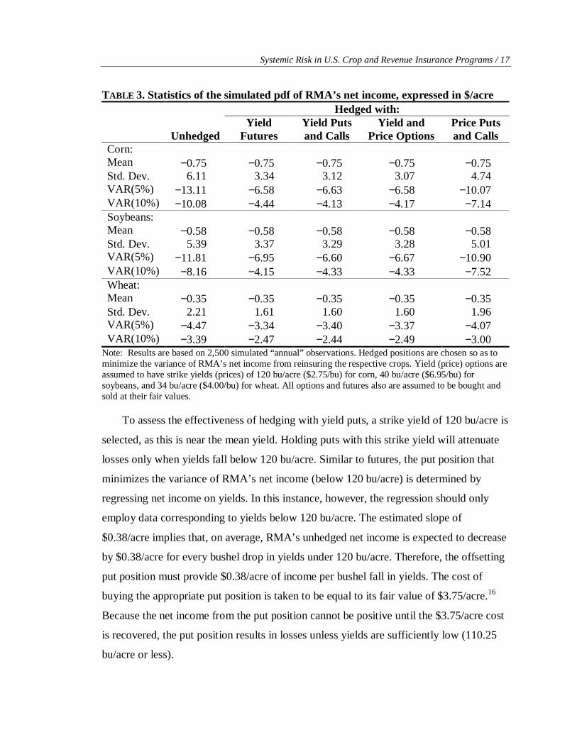
TABLE 3. Statistics of the simulated pdf of RMA’s net income, expressed in $/acreHedged with:

UnhedgedYield

FuturesYield Putsand Calls

Yield andPrice Options

Price Putsand Calls

Corn:Mean −0.75 −0.75 −0.75 −0.75 −0.75Std. Dev. 6.11 3.34 3.12 3.07 4.74VAR(5%) −13.11 −6.58 −6.63 −6.58 −10.07VAR(10%) −10.08 −4.44 −4.13 −4.17 −7.14Soybeans:Mean −0.58 −0.58 −0.58 −0.58 −0.58Std. Dev. 5.39 3.37 3.29 3.28 5.01VAR(5%) −11.81 −6.95 −6.60 −6.67 −10.90VAR(10%) −8.16 −4.15 −4.33 −4.33 −7.52Wheat:Mean −0.35 −0.35 −0.35 −0.35 −0.35Std. Dev. 2.21 1.61 1.60 1.60 1.96VAR(5%) −4.47 −3.34 −3.40 −3.37 −4.07VAR(10%) −3.39 −2.47 −2.44 −2.49 −3.00

Note: Results are based on 2,500 simulated “annual” observations. Hedged positions are chosen so as tominimize the variance of RMA’s net income from reinsuring the respective crops. Yield (price) options areassumed to have strike yields (prices) of 120 bu/acre ($2.75/bu) for corn, 40 bu/acre ($6.95/bu) forsoybeans, and 34 bu/acre ($4.00/bu) for wheat. All options and futures also are assumed to be bought andsold at their fair values.

To assess the effectiveness of hedging with yield puts, a strike yield of 120 bu/acre is

selected, as this is near the mean yield. Holding puts with this strike yield will attenuate

losses only when yields fall below 120 bu/acre. Similar to futures, the put position that

minimizes the variance of RMA’s net income (below 120 bu/acre) is determined by

regressing net income on yields. In this instance, however, the regression should only

employ data corresponding to yields below 120 bu/acre. The estimated slope of

$0.38/acre implies that, on average, RMA’s unhedged net income is expected to decrease

by $0.38/acre for every bushel drop in yields under 120 bu/acre. Therefore, the offsetting

put position must provide $0.38/acre of income per bushel fall in yields. The cost of

buying the appropriate put position is taken to be equal to its fair value of $3.75/acre.16

Because the net income from the put position cannot be positive until the $3.75/acre cost

is recovered, the put position results in losses unless yields are sufficiently low (110.25

bu/acre or less).


Compared to the no-hedging scenario, hedging with yield puts leaves the mean

unchanged17 (at a loss of $0.75/acre) but reduces risk substantially, cutting by almost half

both the standard deviation (from $6.11/acre to $3.17/acre) and VAR(5%) (from a loss of

$13.11/acre to a loss of $7.20/acre). Somewhat unexpectedly, however, the standard

deviation achieved by hedging with yield puts ($3.17/acre) is negligibly smaller than the

standard deviation obtained by hedging with yield futures ($3.34/acre). Even more

perplexing is that VAR(5%) is worse when hedging with puts than when hedging with

futures (losses of $7.20/acre and $6.58/acre, respectively). Further analysis reveals that

the culprit responsible for VAR(5%) being worse for puts than for futures is the high cost

of purchasing the former ($3.75/acre) compared to buying the latter ($0/acre).

From the scatter diagram in Figure 2 it is clear that RMA’s net income is positively

related to yields, for yields above 120 bu/acre. The estimated slope from the correspond-

ing regression is 0.13. This implies that a combination of yield puts and calls should be

more effective in reducing risks than yield puts alone. Focusing on yield puts and calls

with a strike yield of 120 bu/acre, the optimal put position is the same as obtained before;

whereas the optimal call position consists of selling calls so that RMA’s net income is

expected to decrease by $0.13/acre (i.e., the slope estimate) per bushel increase in yields

above 120 bu/acre. The ensuing sale of calls at fair values generates $0.93/acre in

revenues, which, combined with the $3.75/acre cost of the puts, nets a cost of $2.82/acre

for the portfolio of puts and calls.

As expected, hedging with yield puts and calls is more effective in reducing risks

than hedging with puts only. By hedging with both puts and calls instead of puts alone,

the standard deviation of RMA’s net income is reduced from $3.17/acre to $3.12/acre,

and VAR(5%) is improved from a loss of $7.20/acre to a loss of $6.63/acre. It is

important to stress, however, that the risk reduction performance of the put-call portfolio

vis-à-vis hedging with futures seems negligible from a practical standpoint.

It is also relevant to analyze whether price derivatives can be added to the portfolio

of yield derivatives to further mitigate RMA’s net income risk. For example, it is clear

from (4) that CRC indemnities depend directly and in a nonlinear fashion on harvest

prices (Ph). When harvest prices are above planting prices (Pp), CRC indemnities are paid


if (ψCRC Y − y) Ph > 0. In contrast, when harvest prices are below planting prices, CRC

indemnities are paid if (ψCRC Pp Y − Ph y) > 0. Therefore, holding yields constant,

indemnitiesincrease(decrease) by the amountψCRC Y − y > 0 (y > 0) per unit increase in

harvest price if Ph > (<) Pp. In other words, holding yields constant, RMA’s net income is

expected to decline as harvest prices deviate from expected prices.

The preceding analysis suggests that a long position in both price puts and price calls

with a strike price near the planting price (i.e., a bottom straddle or straddle purchase

(Hull, pp. 187–188) would be the most appropriate addition to the portfolio of yield

derivatives. To examine this, RMA’s net income after hedging with yield options is

regressed against futures prices. The hypothesized change in slope sign at the expected

price level is taken care of by running separate regressions for data corresponding to

prices above and below $2.75/bu (the 1997 corn CRC planting price is $2.73). As

expected, the slope is negative (−2.14) and positive (2.41) for prices below and above

$2.75/bu, respectively. Thus, the offsetting position in price options must have a payoff

that decreases by−$2.14/acre (increases by $2.41/acre) for every $1/bu increase in the

harvest price of corn below (above) $2.75/bu.

The fair cost of the offsetting position in price options is $0.78/acre. Adding this

bottom straddle to the portfolio of yield options has very little effect on the pdf of RMA’s

net income (see Table 3). With its inclusion, standard deviation is reduced only slightly to

$3.07/acre, compared to $3.12/acre when using yield options only. VAR(5%) falls from a

loss of $6.63/acre to a loss of $6.58/acre, but VAR(10%) moves from a loss of $4.13/acre

to a loss of $4.17/acre. Looking at the range of outcomes, the maximum loss is reduced

from $18.61/acre to $18.08/acre, whereas the maximum gain is also reduced from

$8.96/acre to $8.65/acre.

Unfortunately, in reality it may be problematic for RMA to use yield derivatives.

This is true because currently there are no yield derivatives for soybeans and wheat.

Further, yield derivatives for corn have languished since their introduction in 1995, and

their market seems too thin for RMA’s hedging needs. For these reasons, and given the

strong correlation between prices and yields (e.g., see subsection “Simulation of Harvest

Prices”), it is of interest to explore the potential of using only price derivatives to hedge

RMA’s net income.


To assess the hedging potential of price derivatives in isolation, it is assumed that

RMA only hedges by means of corn price options with a strike price of $2.75/bu (i.e., the

same strike price used to analyze the portfolio of yield and price derivatives).18 The

portfolio of price options that minimizes the variance of RMA’s net income from

reinsuring corn is obtained by running separate regressions of net income against harvest

prices, for data corresponding to prices above and below $2.75/bu. The estimated slope

for prices above (below) $2.75/bu is−12.03 (−9.62), which implies that the optimum

portfolio involves purchasing calls and selling puts in a ratio of 12.03:9.62.19

Not surprisingly, Table 3 shows that the position in price options is not as effective

at reducing RMA’s net income risk as is the position in yield options. With price options,

the standard deviation is $4.74/acre, compared to $6.11/acre with the naked position and

$3.12/acre with the position in yield options. VAR(5%) is a loss of $10.07/acre, falling

between the unhedged and yield-option-hedged VAR(5%) losses of $13.11/acre and

$6.63/acre. Likewise, VAR(10%) is $7.14/acre for price option hedging, which is better

than the no-hedge VAR(10%) ($10.08/acre) but not as good as VAR(10%) when using

yield options ($4.13/acre).

The effectiveness of hedging RMA’s net income from reinsuring soybeans and

wheat is analyzed using the same methods that are used for corn. It is apparent from the

summary figures reported in Table 3 that results for soybeans and wheat are quite similar

to the results for corn, except for some differences in scale. Therefore, in the interest of

space, discussion of the findings from hedging soybeans and wheat is omitted.

Two major observations can be made after examining the net income from reinsuring

individual crops with and without hedging instruments. The first is that net income

without hedging exhibits wide variability, with small probabilities of very large losses.

This shape of the pdf is altered considerably by hedging with yield and/or price

derivatives. Whereas all pdfs with and without hedging are noticeably skewed to the left,

the no-hedge pdfs exhibit far less kurtosis. The second observation is that, despite the

noticeable risk-reduction effect of holding appropriate positions in derivatives, there

remains a substantial amount of variability in net income after hedging. While the

likelihood of the worst results is much reduced, the range of potential outcomes after

hedging is about the same as before hedging.


For the sake of completeness, the pdf of RMA’s aggregate net income after hedg-

ing is also estimated, imposing historical correlation levels across national crop yields.

It is found that while hedging leaves the mean of aggregate net income unchanged at a

loss of $0.56/acre (due to the assumption that derivatives are fairly priced), it attenuates

variability substantially. For example, hedging with both yield and price options

reduces the standard deviation by more than half (from $3.36/acre to $1.56/acre), and

improves VAR(5%) [VAR(10%)] from a loss of $7.13/acre ($5.52/acre) to a loss of

$3.31/acre ($2.44/acre).

Summary and Conclusions

While crop insurance has received significant attention from economists, there has

been little attempt at quantifying the level of risk accepted by the government in its role

as reinsurer. The present study aims at filling this gap in the literature by estimating the

probability density function (pdf) of the Federal Risk Management Agency’s (RMA) net

income from reinsuring corn, wheat, and soybeans. This is accomplished by means of

Monte Carlo simulations in which correlated yields and prices are drawn and indemnities

are then computed. Using the reinsurance obligations of the RMA, as described in the

1997 Standard Reinsurance Agreement (SRA), payments to and from the RMA are

calculated from indemnity levels.

It is estimated that RMA’s VAR (5%) is $1 billion. That is, there is a 5 percent

probability that RMA will need to reimburse at least $1 billion to insurance companies.

This is a number greater than the reimbursements made by the RMA in its worst

reinsurance year (i.e., 1993), in which claims against the RMA exceeded premiums by

$822 million (U.S. GAO). Another important result is the estimated fair value of RMA’s

reinsurance services to insurance firms. The expected net transfer from RMA to the

insurance industry due to the SRA specifications is estimated at $36.3 million for corn,

$24.6 million for soybeans, and $17.6 million for wheat, for a total of $78.7 million.20

This figure is small compared to potential losses under worst-case scenarios, but it is a

real cost to the government and a real benefit to the insurers.


The question of risk reduction for the reinsurer is also investigated. Assuming the

existence of national yield and price derivatives markets, various hedging strategies are

examined for their potential to reduce RMA’s risks from reinsurance. The level of risk

reduction achievable by hedging is found to be appreciable. For example, hedging with

yield and price options may reduce RMA’s VAR(5%) by more than half, from $1 billion

to $467 million. However, use of these derivative contracts alone is clearly no panacea.

Endnotes

1. In the crop insurance market, diversification does little to mitigate the level of risk (Quiggin). Forexample, Miranda and Glauber computed the coefficient of variation (CV) of indemnity portfoliosowned by the ten largest crop insurance firms, and found that CVs based on historical yield correlationswere between 22 and 49 times larger than CVs based on zero yield correlations. Further, such high CVsdid not seem to be due to poor diversification practices. This level of variability is much higher thanthat seen in other lines of insurance where government participation has not been required.

2. Actual Production History Insurance is also known as Multiple-Peril Crop Insurance.

3. Rank correlations are not affected by monotonic transformations of the underlying variables. Thisbecomes important at the simulation stage, where uniformly distributed random variables are trans-formed into beta-distributed random yields (see next paragraph).

4. In a few low-production counties with small acreages and some missing yield observations (becauseland goes in and out of production over the years) the estimated correlation is negative. These casesare assigned a correlation level of zero in the simulations, because it seems unreasonable that the truecorrelation would be negative.

5. Note that county acreages must include not only insured acres but also uninsured acres.

6. Even if actual data on individual (π, ψ) allocations were available, modeling all of the permitted (π, ψ)combinations for each policy would not be tractable. For example, there are 27 (π, ψ) combinationsfor BUP alone.

7. Calibration begins by fixingψ at its maximum level permitted (ψ = 0.9) and searching for the value ofπ ∈ (0.9, 1.5) that equates the expected loss ratio to one. If this search fails, the process is repeated bysuccessively fixingψ at 0.85, 0.8, 0.75, and 0.7 until aπ ∈ (0.9, 1.5) is found that makes expected lossratios equal to one. When this search also fails, average per-acre GRP indemnities are defined not as(12) but as IGRP(yit) ≡ wGRPi × GRP(yit; 1, ψ GRPi) + (1 – wGRPi) × GRP(yit; 1,ψ GRPi) instead, wherewGRPi ∈ (0, 1),ψ GRPi ∈ ΨGRP, ψ GRPi ∈ ΨGRP, ψGRPi ≠ ψ GRPi, and wGRPi, ψ GRPi, andψGRPi are selectedso that county i’s GRP expected loss ratio equals one. The implicit assumption in using this linearcombination is that a share wGRPi of the GRP acres in county i are insured at coverage levelψ GRPi, andthe rest are insured at coverage levelψ GRPi.

8. There are very few counties for which no CAT policies were sold in 1997, so that their CAT

premiums are zero. In such instances,is is calibrated by using BUP premiums, fixing BUP priceprotection and yield coverage levels atπ = 0.75 andψ = 0.65, respectively, and then proceeding as ifthey were CAT policies.


9. For calibration, an attempt is first made to equate expected indemnities to premiums by fixingψ = 0.65 and adjustingπ. If there is noπ ∈ (0.6, 1.0) which accomplishes this, the same process isrepeated forψ = 0.5 and, if necessary, forψ = 0.75. As with GRP, it is sometimes necessary to use alinear combination of indemnities at two different yield coverage levels because the previous searchprocedure fails to produce expected loss ratios equal to one. In this instance, average per-acre BUP

indemnities are defined as IBUP(yit) ≡ wBUPi [∫ BUP(yit; 1, ψBUPi) dΦ(yait| yit,2

its)] + (1 – wBUPi)

[∫ BUP(yit; 1, ψBUPi) dΦ(yait| yit,2

its)] instead of (15), where wBUPi ∈ (0, 1),ψBUP ∈ ΨBUP, ψBUPi ∈

ΨBUP, ψBUPi ≠ ψBUPi, and wBUPi, ψBUPi, andψBUPi render county i’s BUP1expected loss ratio equal to one.

10. This implies that RMA’s expected net income from reinsurance (without hedging) can also beinterpreted as the negative of insurance firms’ expected net income.

11. Due to the way policies are calibrated, the standard deviation of loss ratios is identical to the CV ofindemnities.

12. A small number of policies cannot be calibrated so as to yield expected loss ratios equal to one,because their expected loss ratios exceed one for all of the permitted coverage levels. Such policiesare calibrated so as to minimize their expected loss ratios within the coverage levels allowed and areassumed to be ceded to the RMA by the insurers. Such instances are confined to counties with veryfew insured acres.

13. VAR(z percent) is merely the dollar value $v such that Probability(net income≤ $v) = z percent(Jorion).

14. More specifically, in each “annual” simulation the historical correlation structure is imposed to drawthe vector of national-level uniformly distributed variablesxUS ≡ [xUS,corn, xUS,soybeans, xUS,wheat] (seesub-subsection “Modeling Systemic County-Level Yield Risk”). This is done using the correlationmatrix, which the @Risk software makes available to the user.

15. Yield futures do currently exist for corn and are traded on the Chicago Board of Trade. Tradedcontracts are based on corn yield estimates of harvested acres made by the National AgriculturalStatistics Service.

16. The $3.75/acre figure would be the put position’s value in the presence of efficient markets (so thatput prices are equal to their expected payoffs). It is obtained by computing the average of the putposition’s payoffs [= 0.38 × max(0, 120 – yUSt)] over 2,500 simulated yield draws.

17. The unchanged mean is an implication that the put position’s cost equals its fair value.

18. To save space, hedging with price futures is not discussed, because put-call parity (Hull, p. 167)implies that any futures position can be replicated by an appropriate combination of puts and callswith the same strike price. Hence, an optimal portfolio of puts and calls will always perform at leastas well as an optimal futures position.

19. Note the striking contrast with the optimal portfolio of yield options, which involved selling calls andbuying puts in a ratio of 0.13:0.38. The reason for such a difference is the negative correlationbetween prices and yields.

20. This is in addition to the administrative and operations expense subsidies that RMA pays to insurancecompanies.


21. The value of N = 26 is the number of annual yield observations per county. Parameter YU isstandardized to 1 to facilitate numerical calculations, as B(y|α, β, YL = 0, YU) = B(z|α, β, YL = 0,YU = 1) for z≡ y/YU. This also implies that the ratio yU/YU is independent of YU, explaining why YU

is not included in the right-hand side of (A.1).

22. For example, the variance of farm-level yields may be greater than usual in drought years, if someproduction units experience very low yields while others are not severely affected by dry weather.

23. For instance, without rescaling, a negative relationship between CVR and county yield would befound if counties with low (high) expected yields have relatively large (small) CVRs.

24. In essence, rescaling is the reverse of the process by which county yields are simulated in the model.

Appendix A: Derivation of Expression (9)

The motivation for (9) is that the maximum value from a sample of N observations from the beta pdf

B(y| α, β, YL, YU), yU(N, α, β, YL, YU) is a random variable that is almost surely smaller than YU. Because

yU(N, α, β, YL, YU) is a negatively biased estimate of YU, a feasible method is needed so as to obtain a better

estimate of YU. To assess the magnitude of the likely bias in the historical data set, preliminary estimates ofαi

( iα ) andβi ( iβ ) were obtained for each county i by settingLiY = 0 and letting U

iY range from Uiy

through 1.5 Uiy . It was found that in all instances 2 <iα < 15, 2 < iβ < 15, and 0 < iα − iβ < 7.

The iα and iβ estimates were used to construct 56 (α, β) pairs spanning the likely range of un-

knownαis andβis in the available data. For each (α, β) pair, 1,000 observations on yU(N = 26,α, β, YL = 0,

YU = 1) were obtained by (1) drawing 26 observations from the corresponding beta pdf,21 (2) obtaining

their maximum value (yU), (3) repeating steps (1) and (2) 1,000 times, and (4) calculating the average from

the 1,000 observations about yU. Letting Uy denote such averages, regression (A.1) was run using

ordinary least squares on the resulting 56 observations:

ln( Uy /YU) = −2.5426** – 0.9442** ln(α) + 1.7203** ln(β) + error, R2 = 0. (A.1)

(0.0449) (0.0259) (0.0207)

In (A.1), numbers between parentheses below coefficient estimates are the respective standard

deviations, and “**” denotes significantly different from zero at the 1 percent level based on the two-tailed

t-statistic. The log-log specification in (A.1) was adopted because it had better fit than alternative

specifications such as linear and log-linear.

Appendix B: Variability of Within-County Yield PDFs

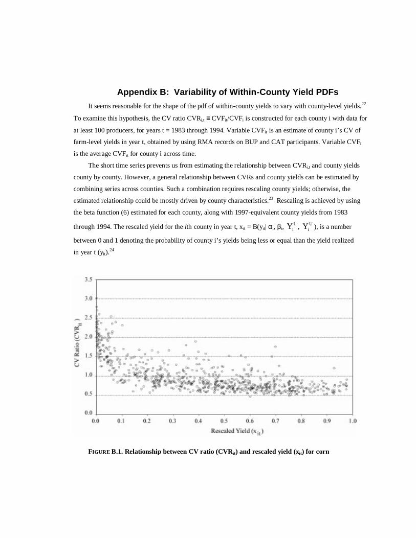
It seems reasonable for the shape of the pdf of within-county yields to vary with county-level yields.22

To examine this hypothesis, the CV ratio CVRi,t ≡ CVFit/CVFi is constructed for each county i with data for

at least 100 producers, for years t = 1983 through 1994. Variable CVFit is an estimate of county i’s CV of

farm-level yields in year t, obtained by using RMA records on BUP and CAT participants. Variable CVFi

is the average CVFit for county i across time.

The short time series prevents us from estimating the relationship between CVRi,t and county yields

county by county. However, a general relationship between CVRs and county yields can be estimated by

combining series across counties. Such a combination requires rescaling county yields; otherwise, the

estimated relationship could be mostly driven by county characteristics.23 Rescaling is achieved by using

the beta function (6) estimated for each county, along with 1997-equivalent county yields from 1983

through 1994. The rescaled yield for theith county in year t, xit = B(yit| αi, βi,L

iY , UiY ), is a number

between 0 and 1 denoting the probability of county i’s yields being less or equal than the yield realized

in year t (yit).24

FIGURE B.1. Relationship between CV ratio (CVRit) and rescaled yield (xit) for corn


Figure B.1 displays a scatter plot of CVRs versus x’s for corn. Analogous scatter plots for soybeans

and wheat display very similar patterns and are omitted in the benefit of space. From Figure B.1, it can be

observed that CVR tends to decrease at a decreasing rate as x rises, and that the dispersion of CVR data

points varies inversely with the level of x. To model such patterns, regressions of the logarithm of CVR

against x were run by weighted least squares, using as weights the predicted squared errors from ordinary

least squares regressions of the logarithm of CVR versus x. Regression results are reported in Table B.1 for

all three crops, where the weighted least squares regression is shown as model 3. The visual patterns

observed in the CVR-x scatter plots are strongly significant. The estimated coefficients for models 2 and 3

in Table B.1 are plugged into equation (14) to calculate the variances of acre-level yields.

TABLE B.1. Regression estimates of the relationship between CV ratio (CVRit) and rescaled yield (xit)Regression Models:a

1. ln(CVRit) = b10 + b11 xit + e1it.

2. 21ite = b20 + b21 xit + e2it, where 1ite ≡≡≡≡ ln(CVR it) −−−− 10b −−−− 11b xit.

3. ln(CVRit)/( 20b + 21b xit)0.5 = b30 + b31 xit + e3it.

Corn Soybeans Wheat

Model 1: 10b 0.3983** 0.3473** 0.3127**

(0.0169)b (0.0183) (0.0173)

11b −0.8280** −0.9938** −0.8279**

(0.0261) (0.0363) (0.0318)R2 0.510 0.508 0.410No.observations 971 730

544

Model 2: 20b 0.1087** 0.0954** 0.1048**

(0.0084) (0.0065) (0.0070)

21b −0.0792** −0.0619** −0.0597**

(0.0131) (0.0128) (0.0128)R2 0.037 0.031 0.039Wc 35.51** 22.66** 21.37**No.observations 971 730 544

Model 3: 30b 1.3907** 1.2520** 1.0745**

(0.0619) (0.0660) (0.0607)

31b −3.3074** −3.9242** −3.0749**

(0.0956) (0.1309) (0.1115)R2 0.553 0.553 0.438No.observations 971 730 544

Note: ** denotes significantly different from zero at the 1% level based on the two-tailed t-statistic.aVariables with hats ( ) denote sample estimates. Variables e1it, e2it, and ei3t are errors.bNumbers between parentheses below coefficient estimates are the respective standard deviations.cW is the critical value for the heteroskedasticity test developed by White, which is distributed as

2

1χ .

References

Babcock, B. A., and D. A. Hennessy. 1996. “Input Demand under Yield and Revenue Insurance.”American Journal of Agricultural Economics78(May): 416-27.

Ederington, L. H. 1979. “The Hedging Performance of the New Futures Markets.”Journal of Finance34:157-70.

Gallagher, P. 1987. “U.S. Soybean Yields: Estimation and Forecasting with Nonsymmetric Disturbances.”American Journal of Agricultural Economics69(November) :796-803.

Gardner, B. L., and R. A. Kramer. 1986. “Experience with Crop Insurance Programs in the United States.”In Crop Insurance for Agricultural Development: Issues and Experience, P. Hazell, C. Pomareda,and A. Valdes, eds. Baltimore, MD: The Johns Hopkins University Press.

Hull, J. C. 1997.Options, Futures, and Other Derivatives,3rd ed. Upper Saddle River, NJ: Prentice Hall.

Johnson, M. E., and A. Tenenbein. 1981. “A Bivariate Distribution Family with Specified Marginals.”Journal of the American Statistical Association76(March): 198-201.

Johnson, N. L., and S. Kotz. 1970.Continuous Univariate Distributions. New York: John Wiley.

Jorion, P. 1997.Value at Risk.New York: McGraw-Hill.

Just, R. E., and Q. Weninger. 1990. “Are Crop Yields Normally Distributed?”American Journal ofAgricultural Economics81(May): 287-304.

Kramer, R. A. 1983. “Federal Crop Insurance, 1938-1982.”Agricultural History57: 181-200.

McClave, J. T., and P. G. Benson. 1988.Statistics for Business and Economics,4th ed. San Francisco:Dellen Publishing Company.

Miranda, M. J., and J. Glauber. 1997. “Systemic Risk, Reinsurance, and the Failure of Crop InsuranceMarkets.” American Journal of Agricultural Economics79(February): 206-15.

Nelson, C. H., and P. V. Preckel. 1989. “The Conditional Beta Distribution As a Stochastic ProductionFunction.” American Journal of Agricultural Economics71(May): 370-78.

Quiggin, J. 1994. “The Optimal Design of Crop Insurance.” InEconomics of Agricultural Crop Insurance:Theory and Evidence, D. L. Hueth and W. H. Furtan, eds. Boston: Kluwer Academic Publishers,pp. 115-33.

Ramirez, O. A. 1997. “Estimation and Use of a Multivariate Parametric Model for SimulatingHeteroskedastic, Correlated, Nonnormal Random Variables: The Case of Corn Belt Corn, Soybeans,and Wheat Yields.”American Journal of Agricultural Economics79(February): 191-205.

U.S. Department of Agriculture, National Agricultural Statistics Service (USDA-NASS).County LevelData. http://www.nass.usda.gov:81/ipedbcnty/main2.htm.


U.S. Department of Agriculture, Risk Management Agency (USDA-RMA).RMA Manager’s Bulletin.Various issues.http://www.act.fcic.usda.gov/news/managers/.

U.S. General Accounting Office (U.S. GAO). 1998. “Crop Revenue Insurance: Problems with New PlansNeed to be Addressed.” GAO/RCED-98-111. Washington, D.C.: United States General AccountingOffice, April. http://www.gao.gov/AIndexFY98/abstracts/rc98111.htm.

Vaughan, E. J., and T. M. Vaughan. 1996.Fundamentals of Risk and Insurance. New York: John Wiley& Sons.

systemic risk in u.s. crop and revenue insurance programs · systemic risk in u.s. crop and revenue...

Documents