system simulation (18790)
TRANSCRIPT

Queuing Simulation SS2015 Simulation of Queuing System Matriculation Nr. 18790 Muhammad Ahsan Nawaz 7/10/2015

Queuing Simulation
1
Abstract
The type of queuing system a business uses is an important factor in determining how efficient
the business is run. In this project, we examine one type of queue system: single-server queue
system which is commonly seen in grocery stores, call centers, banks and fast food restaurants
respectively. We use computer programs to simulates the queues and predict the queue length,
waiting time and wait probability. The input to the simulation program is based on the statistics
collected from different possibilities. The discrete–event simulation approach is used to model
the queuing systems and to analyze the side effects when one system is changed to other. Finally, with
comparative analysis of experiment data, we show that under a special condition, the
difference of the performance of the queuing systems with different queuing disciplines is
limited.

Queuing Simulation
2
Revision History
Name Date Reason for changes Version
Simulation of queuing system
13-11-2015 First time(Just Completed) 1.0
Simulation of queuing system
14-11-2015 Minor changes 1.1

Queuing Simulation
3
Table of Contents:
CHAPTER – 1 Introduction ----------------------------------------------------------------------------------------------------- 5
1. Introduction --------------------------------------------------------------------------------------------------------------------- 6
1.1. What is it? ----------------------------------------------------------------------------------------------------------------- 6
CHAPTER – 2 Problems ---------------------------------------------------------------------------------------------------------- 8
2. Simulation of Queuing System: why? ----------------------------------------------------------------------------------- 9
2.1. Single-Server Queuing System: ------------------------------------------------------------------------------------ 10
2.2. Components of Queuing System:--------------------------------------------------------------------------------- 10
CHAPTER – 3 Models ------------------------------------------------------------------------------------------------------------ 11
3. Models: -------------------------------------------------------------------------------------------------------------------------- 12
3.1. Simulation using tables: --------------------------------------------------------------------------------------------- 12
3.1.1. Simulation steps using Simulation tables: -------------------------------------------------------------- 12
3.1.2. Simulation of Queuing system ------------------------------------------------------------------------------ 12
3.1.3. Interesting Observations ------------------------------------------------------------------------------------- 16
3.2. Examples: ---------------------------------------------------------------------------------------------------------------- 16
3.2.1. Example 1: A Grocery ------------------------------------------------------------------------------------------ 17
3.2.2. Example 2: Call Center Problem ---------------------------------------------------------------------------- 20
CHAPTER – 4 Results ------------------------------------------------------------------------------------------------------------ 24
4. Results: -------------------------------------------------------------------------------------------------------------------------- 25
4.1. Discussion of the results: -------------------------------------------------------------------------------------------- 25
4.2. Advantages of Queuing System Simulation: ------------------------------------------------------------------ 26
4.3. Disadvantages: --------------------------------------------------------------------------------------------------------- 26
Summary: ------------------------------------------------------------------------------------------------------------------------------ 27
Critical reflection: ------------------------------------------------------------------------------------------------------------------- 27
Literature: ----------------------------------------------------------------------------------------------------------------------------- 28
References: ---------------------------------------------------------------------------------------------------------------------------- 28

Queuing Simulation
4
List of Figures:
Figure 1: Queuing System ---------------------------------------------------------------------------------------------------------- 6
Figure 2: Simulation of Queuing system: Why? ------------------------------------------------------------------------------ 9
Figure 3: Flow chart of arrival event ------------------------------------------------------------------------------------------- 13
Figure 4: Flow chart of departure event -------------------------------------------------------------------------------------- 14
Figure 5: Chart of number of customer in the system -------------------------------------------------------------------- 16
Figure 6: A Grocery ------------------------------------------------------------------------------------------------------------------ 17
Figure 7:Call center ------------------------------------------------------------------------------------------------------------------ 20
Figure 8: Graph for call center --------------------------------------------------------------------------------------------------- 23
Figure 9: Graph for Bin frequency ---------------------------------------------------------------------------------------------- 23
List of Tables:
Table 1: Simulation using table -------------------------------------------------------------------------------------------------- 12
Table 2: Simulation of queuing system (1) ----------------------------------------------------------------------------------- 15
Table 3: Simulation of queuing system (2) ----------------------------------------------------------------------------------- 15
Table 4: Chronological ordering of events ------------------------------------------------------------------------------------ 15
Table 5: Analysis of a small grocery store (1) -------------------------------------------------------------------------------- 17
Table 6: Analysis of a small grocery store (2) -------------------------------------------------------------------------------- 18
Table 7: Simulation runs for 100 customers --------------------------------------------------------------------------------- 18
Table 8: Call center problem ----------------------------------------------------------------------------------------------------- 21
Table 9: Service time distribution of baker ----------------------------------------------------------------------------------- 21
Table 10: Service time distribution of Able----------------------------------------------------------------------------------- 21
Table 11: Simulation runs for 100 calls ---------------------------------------------------------------------------------------- 22
Queuing Simulation
5
CHAPTER – 1 Introduction

Queuing Simulation
6
1. Introduction
Queuing simulation is based on the idea of queuing theory that stems from operations
research and helps to analyze and model resource allocation and process duration for a
variety of different applications.
1.1. What is it?
Queuing simulation as a method is used to analyze how systems with limited
distribute those resources to elements waiting to be served, while waiting elements
may exhibit discrete variability in demand, i.e. arrival times and require discrete
processing time.
Queuing theory based analysis is regularly used for e.g. A Grocery, Call Center and
Banks. A queuing system is described by its calling population, the nature of the
arrivals, the service mechanism, the system capacity, and the queuing discipline. A
simple single-channel queuing system is portrayed in Figure 1.Whether, Different
queuing models are possible; however, all follow the structure of:
Calling Population
Waiting Line
Server
Figure 1: Queuing System
Source: http://www.me.utexas.edu/~jensen/ORMM/computation/unit/dynamic_programming/dp_data/finite_queue/

Queuing Simulation
7
Figure: 1 clearly shown the whole procedure of single-Channel queuing system. And
a queuing system is described by:
Calling Population
Arrival Rate
Service mechanism
System capacity
Queuing discipline
Queuing Simulation
8
CHAPTER – 2 Problems

Queuing Simulation
9
2. Simulation of Queuing System: why?
Figure 2: Simulation of Queuing system: Why?
Source: http://blogs.citrix.com/2013/06/28/efficient-queuing-but-where/
There are many reasons behind this phenomena that why we need Queuing simulation?
Some of the factor’s discussed in this paper.
Here is some factor’s:
A major application of simulation has been in the analysis of waiting line, or
queuing systems.
Since the time spent by people and things waiting in line is a valuable resource,
the reduction of waiting time is an important aspect of operations management.
Waiting time has also become more important because of the increased
emphasis on quality. Customers equate quality service with quick service and
providing quick service has become an important aspect of quality service.
Capacity problem are very common in industry and one of the main drivers of
process redesign.
Need to balance the cost of increased capacity against the gains of
increased productivity and service.
Queuing and waiting time analysis is particularly important in service systems.
Large costs of waiting and of lost sales due to waiting.

Queuing Simulation
10
Example:
Patients arrive by ambulance or by their own record.
One doctor is always on duty
More and more patient seeks help Longer waiting times
Questions: should another MD position be instated?
2.1. Single-Server Queuing System:
The single channel queuing system can be seen in places such as banks, post offices,
Grocery stores and call centers, where one single queue will diverge into a few
counters. The moment a customer leaves a service station, the customer at the head
of the queue will go the server. The disadvantage of a Single-channel queue is that
the queue length seems to be very long, thus it can discourage customers to join the
queue.
2.2. Components of Queuing System:
A queue system can be divided into four components:
Arrivals: Concerned with how items (People, cars etc.) arrive in the system.
Queue or waiting line: Concerned with what happens between the arrival of
an item requiring service and the time when service is carried out.
Service: Concerned with the time taken to serve a customer.
Outlet or departure: The exit from the system.
A queuing problem involves striking a balance between the cost of making
reductions in service time and the benefits gained from such a reduction.

Queuing Simulation
11
CHAPTER – 3 Models

Queuing Simulation
12
3. Models: There are many ways to simulate queuing system by using tables, MS Excel or through
different software like; Arena, Witness and R Studio. But in this paper we will go to
discuss queuing system simulation by using Tables and MS Excel.
3.1. Simulation using tables:
Introducing simulation by manually simulating on a table
Can be done via pen-and-paper or by using a spreadsheet
Table 1: Simulation using table
Repetition Inputs Response
I Xi1 Xi2 … Xij … Xip Yi
1
2
. . .
N
3.1.1. Simulation steps using Simulation tables:
Determine the characteristics of each of the inputs to the simulation. Quite
often, these may be modeled as probability distributions, either continuous or
discrete.
Construct a simulation table. Each simulation table is different, for each is
developed for the problem at hand. Example: there are p inputs, xij; J = 1, 2… p
and one response, Yi, for each of repetitions I = 1, 2… n. Initialize the table by
filling in the data for repetition 1.
For each repetition I, generate a value for each of the p inputs, and evaluate the
function, calculating a value of the response Yi. The input values may be
computed by sampling values from the distributions determined in step 1. A
response typically depends on the inputs and one or more previous responses.
Determine the characteristics of each of the inputs to the simulation (Probability
distribution).
3.1.2. Simulation of Queuing system
Single server queue
Calling population is infinite

Queuing Simulation
13
o Arrival rate does not change
Units are served according FIFO.
Arrivals are defined by the distribution of the time between
Arrivals inter- arrival time
Service times are according to a distribution
Arrival rate must be less than service rate stable system
Otherwise waiting line will grow unbounded unstable system.
Queuing system state
System
o Server
o Units (in Queue or being served)
o Clock
State of the system
o Number of units in the system
o Status of server (idle, busy)
Events
o Arrival of a unit
o Departure of a unit
Flow chart (Arrival Event)
If server idle unit gets service, otherwise unit enters queue.
Figure 3: Flow chart of arrival event
The arrival event occurs when a unit enters the system. The unit may find the server
either idle or busy; therefore, either the unit begins service immediately, or it enters the
queue for the server.

Queuing Simulation
14
Flow Chart (Departure Event)
If queue is not empty begin servicing next unit, otherwise server will be idle.
Figure 4: Flow chart of departure event
If a unit has just completed service, the simulation proceeds in the manner shown in the
flow diagram of Figure 3.0. Note that the server has only two possible states: it is either
busy or idle.
How do events occur?
Events occur randomly
Inter-arrival times = {1,…,6}
Service times = {1,…,4}

Queuing Simulation
15
Table 2: Simulation of queuing system (1)
Customer Inter-arrival Time Arrival time on clock Service Time
1 - 0 2 2 2 2 1
3 4 6 3
4 1 7 2 5 2 9 1
6 6 15 4
Table 3: Simulation of queuing system (2)
Customer Number
Arrival Time [Clock]
Time Service Begins [Clocks]
Service Time [Duration]
Time Service Ends [clock]
1 0 0 2 2
2 2 2 1 3 3 6 6 3 9
4 7 9 2 11
5 9 11 1 12 6 15 15 4 19
Table 4: Chronological ordering of events
Clock Time Customer Number Event Type Number of Customers
0 1 Arrival 1
2 1 Departure 0
2 2 Arrival 1
3 2 Departure 0
6 3 Arrival 1
7 4 Arrival 2
9 3 Departure 1
9 5 Arrival 2
11 4 Departure 1
12 5 Departure 0
15 6 Arrival 1
19 6 Departure 0
The inter-arrival and service time
are taken from distributions
The simulation run is
built by meshing
clock, arrival and
service times!
Queuing Simulation
16
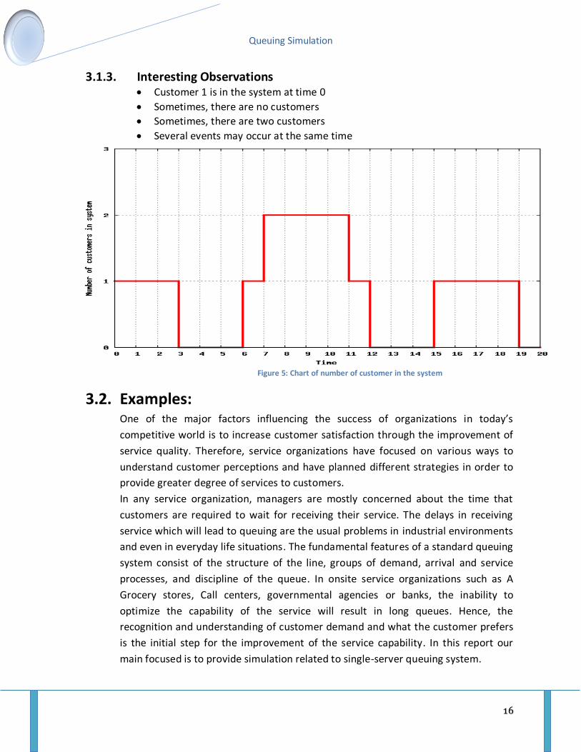
3.1.3. Interesting Observations Customer 1 is in the system at time 0
Sometimes, there are no customers
Sometimes, there are two customers
Several events may occur at the same time
Figure 5: Chart of number of customer in the system
3.2. Examples: One of the major factors influencing the success of organizations in today’s
competitive world is to increase customer satisfaction through the improvement of
service quality. Therefore, service organizations have focused on various ways to
understand customer perceptions and have planned different strategies in order to
provide greater degree of services to customers.
In any service organization, managers are mostly concerned about the time that
customers are required to wait for receiving their service. The delays in receiving
service which will lead to queuing are the usual problems in industrial environments
and even in everyday life situations. The fundamental features of a standard queuing
system consist of the structure of the line, groups of demand, arrival and service
processes, and discipline of the queue. In onsite service organizations such as A
Grocery stores, Call centers, governmental agencies or banks, the inability to
optimize the capability of the service will result in long queues. Hence, the
recognition and understanding of customer demand and what the customer prefers
is the initial step for the improvement of the service capability. In this report our
main focused is to provide simulation related to single-server queuing system.

Queuing Simulation
17
3.2.1. Example 1: A Grocery
Figure 6: A Grocery
Source:https://www.google.com.pk/search?q=queuing+system+images&biw=1366&bih=667&tbm=isch&tbo=u&so urce=univ&sa=X&ved=0CBoQsARqFQoTCOKpsp7V2sYCFQfRFAodH3wPwA#tbm=isch&q=Grocery+store+queuing++system+images&imgrc=LIaBzzsA7LZ7_M%3A
Analysis of a small grocery store One checkout counter
Customer arrives at random times from {1, 2… 8}
Service times vary from {1,2,…,6} minutes
Consider the system for 100 customers
Table 5: Analysis of a small grocery store (1)
Inter-arrival time [minute]
Probability Cumulative Probability
1 0.125 0.125
2 0.125 0.250
3 0.125 0.375
4 0.125 0.500
5 0.125 0.625
6 0.125 0.750
7 0.125 0.875
8 0.125 1.000

Queuing Simulation
18
Table 6: Analysis of a small grocery store (2)
Problems/Simplification
Sample size is too small to be able to draw reliable conclusions
Initial condition is not considered
Simulation runs for 100 Customer
Simulation System Performance Measure
Customer Inter-arrival Time [Minutes]
Arrival Time [Clock]
Time Service Begins [Clock]
Time service Ends [Clocks]
Waiting time in Queue [Minutes]
Time Customer in system [Minutes]
Idle time of server [Minutes]
1 - 0 4 0 4 0 4 0
2 Service time [Minutes]
1 2 4 6 3 5 0
3 1 2 5 6 11 4 9 0
4 6 8 4 11 15 3 7 0
5 3 11 1 15 16 4 5 0
6 7 18 5 18 23 0 5 2
… 100 5 415 2 416 418 1 3 0
Total 415 317 174 491 101 Table 7: Simulation runs for 100 customers
Service Time Probability Cumulative probability
1 010 0.10
2 0.20 0.30
3 0.30 0.60
4 0.25 0.85
5 0.10 0.95
6 0.05 1.00

Queuing Simulation
19
Example 1: A Grocery, Some Statistics
Average Waiting Time
w = ∑ Waiting Time in queue/No. of Customers = 174/100 = 1.74 min
Probability that a customer has to wait
p(wait) = No. of customer who wait/No. of customers = 46/100 = 0.46
Proportion of server idle time p(idle server) = Σ Idle time of server/Simulation run time = 101/418 = 0.24
Average service time s = Σ Service Time /Number of customers = 317/100 = 3.17 min E(s) =∑
s*p(s) = 0.1*10+0.2*+…+0.05* = 3.2 min
Average time between arrivals λ = ∑ Time between arrivals/No. of arrivals – 1 = 415/99 = 4.19 min E (λ) = a+b/2 = 1+8/2 = 4.5 min
Average waiting time of those who wait
W waited = ∑ Waiting time in queue/No. of customers that wait = 174/54 = 3.22 min
Average time a customer spends in system
t = ∑ Time customers spend in system/Number of customers = 491/100 = 4.91 min
t = w + s = 1.74 + 3.17 = 4.91 min A Grocery, Some Statistics
Interesting results for a manager, but
Longer simulation run would increase the accuracy

Queuing Simulation
20
3.2.2. Example 2: Call Center Problem
Figure 7: Call center
Source: https://www.linkedin.com/pulse/call-center-simulation-fix-without-breaking-jeffrey
Call center Problem:
Consider a call center where technical personnel take calls and provide service
Two technical support people (2server) exists
Able more experienced, provides service faster
Baker Newbie, provides service slower
Rule
Able gets call if both people are idle
Try other rules
Baker gets call if both are idle
Call is assigned randomly to Able and Baker
Goal of study: Find out how well the current rule works
Inter-arrival distribution of calls for technical support

Queuing Simulation
21
Table 8: Call center problem
Time between Arrivals [Minute]
Probability Cumulative Probability
Random-Digit Assignment
1 0.25 0.25 01 – 25
2 0.40 0.65 26 – 65
3 0.20 0.85 66 – 85
4 0.15 1.00 86 – 00
Service time distribution of baker
Service Time [Minute]
Probability Cumulative Probability
Random-Digit Assignment
3 0.35 0.35 01 – 35
4 0.25 0.60 36 – 60
5 0.20 0.80 61 – 80
6 0.20 1.00 81 – 00 Table 9: Service time distribution of baker
Service time distribution of Able
Service Time [Minute]
Probability Cumulative Probability
Random-Digit Assignment
2 0.30 0.30 01 – 30
3 0.28 0.58 31 – 58
4 0.25 0.83 59 – 83
5 0.17 1.00 84 – 00 Table 10: Service time distribution of Able
Simulation Proceeds as follows:
Step 1:
For caller k, generate an inter-arrival time A(k). Add it to the previous arrival time
T (K-1) to get arrival time of caller k as T(k) = T (K-1) + A(k)
Step 2:
If Able is idle, caller k begins service with Able at the current time T(now)
Able’s service completion time T (fin, A) is given by T (fin,A) = T (now) + T(svc,A)
Where T(svc,A) is the service time generated from Able’s service time
distribution. Caller k’s waiting time is T (wait) = 0.
Caller K’s time in system, T(sys), is given by T(sys) = T(fin,A) – T(k)
If Able is busy and Baker is idle, Caller begins with Baker. The remainder is in
analogous.

Queuing Simulation
22
Step 3:
If Able and Idle are both busy, then calculate the time at which the first one
becomes available, as follows: T (beg) = min (T (fin,A), T(fin,B)).
Caller k begins service at T(beg). When service for caller K begins, set T(now) = T
(beg).
Compute T (fin,A) or T (fin,B) as in step 2.
Caller K’s time in system is T(sys) = T(fin,A) – T(k) or T (sys) = T(fin,B) – T(k).
Simulation runs for 100 Calls:
Caller Nr.
Inter-arrival Time
Arrival Time
When Able Avail.
When Baker Avail
Server chosen
Service Time
Time Service Begins
Able’s Service Compl. Time
Baker’s Service Compl. Time
Caller Delay
Time in system
1 - 0 0 0 Able 2 0 2 0 2
2 2 2 2 0 Able 2 2 4 0 2
3 4 6 4 0 Able 2 6 8 0 2
4 2 8 8 0 Able 4 8 12 0 4
5 1 9 12 0 Baker 3 9 12 0 3
… … … … … …
100 1 219 221 219 Baker 4 219 0 4
Total 211 564 Table 11: Simulation runs for 100 calls
Some Statistics:
One simulation trial of 100 caller
62% callers had no delay
12% callers had a delay of 1-2 minutes

Queuing Simulation
23
Figure 8: Graph for call center
400 simulation trials of 100 caller
80.5% of callers had delay up to 1 minute
19.5% of callers had delay more than 1 minute
Figure 9: Graph for Bin frequency

Queuing Simulation
24
CHAPTER – 4 Results

Queuing Simulation
25
4. Results: Given tables show the simulation results. As observed in the above mentioned tables,
the server utilization remains fairly constant as the total workload does not changed.
4.1. Discussion of the results:
In simulation statistical (and probability) theory plays a part both in relation to the input data and in relation to the results that the simulation produces. For example in a simulation of the flow of people through supermarket checkouts input data like the amount of shopping people have collected is represented by a statistical (probability) distribution and results relating to factors such as customer waiting times, queue lengths, etc. are also represented by probability distributions. In our simple example above we also made use of a statistical distribution - the uniform distribution.
There are a number of problems relating to simulation models:
Typically the simulation model has to be run on the computer for a considerable time in order for the results to be statistically significant - hence simulations can be expensive (take a long time) in terms of computer time
Results from simulation models tend to be highly correlated meaning that estimates derived from such models can be misleading. Correlation is a statistical term meaning that two (or more) variables are related to each other in some way. Often variance reduction techniques can be used to improve the accuracy of estimates derived from simulation.
In the event that we are modeling an existing system it can be difficult to validate the model (computer program) to ensure that it is a correct representation of the existing system
If the simulation model is very complex then it is difficult to isolate and understand what is going on in the model and deduce cause and effect relationships.
Once we have the model we can use it to:
Understand the current system, typically to explain why it is behaving as it is. For example if we are experiencing long delays in production in a factory then why is that - what factors are contributing to these delays?
Explore extensions (changes) to the current system, typically to try and improve it. For example if we are trying to increase the output from a factory we could:
Add more machines; or Speed up existing machines; or

Queuing Simulation
26
Reduce machine idle time by better maintenance.
Which of these factors (or combination of factors) will be the best choice to increase output? Note here that any change might reduce congestion at one point only to increase it at another point so we have to bear this in mind when investigating any proposed changes.
Design a new system from scratch, typically to try and design a system that satisfies certain (often statistical) requirements at minimum cost. For example in the design of an airport passenger terminal what resource levels (customs, seats, baggage facilities, etc.) do we need and how should they be sited in relation to one another.
4.2. Advantages of Queuing System Simulation:
The advantages of using simulation, as opposed to queuing theory are:
It can more easily deal with time-dependent behavior The mathematics of queuing theory is hard and only valid for certain statistical
distributions - whereas the mathematics of simulation is easy and can cope with any statistical distribution
In some situations it is virtually impossible to build the equations that queuing theory demands (e.g. for features like queue switching, queue dependent work rates)
Simulation is much easier for managers to grasp and understand than queuing theory.
4.3. Disadvantages:
One disadvantage of simulation is that it is difficult to find optimal solutions, unlike linear programming where we have an algorithm which will automatically find an optimal solution. The only way to attempt to optimize using simulation is to:
Make a change; and Run the simulation computer program to see if an improvement has been
achieved or not; and Repeat.
Large amounts of computer time can be consumed by this process.

Queuing Simulation
27
Summary: The paper considers the queuing system & we could go expanding our models of
queuing systems to represent increasingly complex and realistic situations. But this is
beyond our scope. There are many resources available on how queuing models can be
used to understand the behavior of manufacturing systems.
While the single server queuing situations considered in this chapter are simple, they
yield some fundamental insights that extend well beyond these simple settings. Many of
other things involved in it like:
This report introduced simulation concepts by means of examples.
Examples simulations were performed on a table manually
Use a spreadsheet for large experiments (Excel, open-office)
Input data is important
Random variables can be used.
Output analysis important and difficult
The used tables were of ad hoc, a more methodic approach is needed.
Critical reflection: Modeling uncertain Single server queuing systems is difficult but vitally important
practical problem. Exact computations are often either impossible or very challenging
computationally, especially with multiple customer types. Special challenges are present
when deciding on a service policy in order to make the system as efficient as possible.
In this paper we have presented several approximation procedures that are
computationally easy and, at least in the examples we have looked at, provide valuable
information about the efficiency of the service system under different service options.
An important feature of these approximations is that they stay computationally feasible
even for many task types and/or heavily loaded systems.
This policy has performed well under scenarios we have considered. A number of
important issues are left for future work. One such issue is improving the single-server
queuing system and also implements different approaches in Multiple-based queue
system. Another untouched issue is that of non-stationary: what happens if the
parameters of the system change with time, and need to be constantly estimated in
order to update the service policy and keep the system running efficiently. We hope to
address the latter question in the near future.

Queuing Simulation
28
Literature: Well, we admit there are many of flaws in this report but we can use this report for further
progress. The simulation of queuing system can be applied to many real-world applications from
car parking in multiple–story car parks to ship docking at seaports. If it were possible to improve
the queues, there would be more profits made and more time to carry out business than ever
before, which would be very useful in this fast paced world.
References: [1] Buzacott, J., J.G. Shantikumar. 1993. Stochastic Models of Manufacturing Systems.
PrenticeHall, Englewood Cliffs, NJ.
[2] Carmichael, D.G. 1987. Engineering Queues in Construction and Mining. Halsted
Press/Ellis Horwood Ltd., London.
[3] Çinlar, E. 1975. Introduction to Stochastic Processes. Prentice-Hall, New York.
[4] Hopp, W., M. Spearman. 2000. Factory Physics: Foundations of Manufacturing
Management. McGraw-Hill, New York.
[5] D. Jerry Banks, John S. Carson, Discrete-Event System Simulation, Prentice Hall.
[6] K. Watkins, Discrete Event Simulation in C, McGraw-Hill.
[7] Courtois, P.J., and Georges, J., “On a Single Server Finite Capacity Queueing Model
with State dependent Arrival and Service Process”, Operations Research. 19 (1971) 424-
435.
[8] Raynolds, J.F., “The stationary solution of a multi-server queueing model with
discouragement”, Operations research, 16 (1968) 64-71.
[9] Kleinrock, L. 1975. Queueing Systems, Volume 1. Wiley, New York.
[10] Saltzman, R, V. Mehrotra. 2001. A Call Center Uses Simulation to Drive Strategic
Change. Interfaces 31(3), 87–101.