system models : transformations on vector spacesdorny/vectorsp/systemmodels33-92.pdfsystem models :...
TRANSCRIPT

2
System Models :Transformations
on Vector Spaces
The fundamental purpose in modeling a system is to develop a mechanismfor predicting the condition or change in condition of the system. In theabstract model TX =y of (1.1), T represents (or is a model of) the system,whereas x and y have to do with the condition of the system. We explorefirst some familiar models for the condition or changes in condition ofsystems. These examples lead us to use a generalization of the usual notionof a vector as a model for the condition of a system. We then develop theconcept of a transformation of vectors as a model of the system itself. Therest of the chapter is devoted to examination of the most commonly usedmodels-linear models-and their matrix representations.
2.1 The Condition of a System
The physical condition (or change in condition) of many simple systemshas been found to possess a magnitude and a direction in our physicalthree-dimensional space. It is natural, therefore, that a mathematicalconcept of condition (or change in condition) has developed over timewhich has these two properties; this concept is the vector. Probably themost obvious example of the use of this concept is the use of arrows in atwo-dimensional plane to represent changes in the position of an object onthe two-dimensional surface of the earth (see Figure 2.1). Using the usualtechniques of analytic geometry, we can represent each such arrow by apair of numbers that indicates the components of that arrow along each ofa pair of coordinate axes. Thus pairs of numbers serve as an equivalentmodel for changes in position.
An ordinary road map is another model for the two-dimensional surfaceof the earth. It is equivalent to the arrow diagram; points on the map are
33

34 System Models: Transformations on Vector Spaces
Figure 2.1. An “arrow vector” diagram.
equivalent to the arrow tips of Figure 2.1. The only significant differencebetween these two models is that the map emphasizes the position (orcondition) of an object on the earth, whereas the arrow diagram stressesthe changes in position and the manner in which intermediate changes inposition add to yield a total change in position. We can also interpret aposition on the map as a change from some reference position. Themanner in which we combine arrows or changes in position (the paral-lelogram rule) is the most significant characteristic of either model. Con-sequently we focus on the arrow model which emphasizes the combinationprocess.
Reference arrows (coordinate axes) are used to tie the arrow model tothe physical world. By means of a reference position and a pair ofreference “position changes” on the surface of the earth, we relate thepositions and changes in position on the earth to positions and arrows inthe arrow diagram. However, there are no inherent reference axes on eitherthe physical earth or the two-dimensional plane of arrows.
The same vector model that we use to represent changes in position canbe used to represent the forces acting at a point on a physical object. Thereason we can use the same model is that the magnitudes and directions offorces also combine according to the parallelogram rule. The physicalnatures of the reference vectors are different in these three situations: inone case they are changes in position on the earth, in another they arearrows, in the third, forces. Yet once reference vectors are chosen in each,all three situations become in some sense equivalent; corresponding toeach vector in one situation is a vector in the other two; corresponding toeach sum of vectors in one is a corresponding sum in the other two. Weuse the set of arrows as a model for the other two situations because it isthe most convenient of the three to work with.
The set of complex numbers is one more example of a set of objectswhich is equivalent to the set of arrows. We usually choose as references in
Sec. 2.1 The Condition of a System 35
the set of complex numbers the two numbers 1 and i. Based on thesereference numbers and two reference arrows, we interpret every arrow as acomplex number. Here we have one set of mathematical (or geometrical)objects serving as a model for another set of mathematical objects.
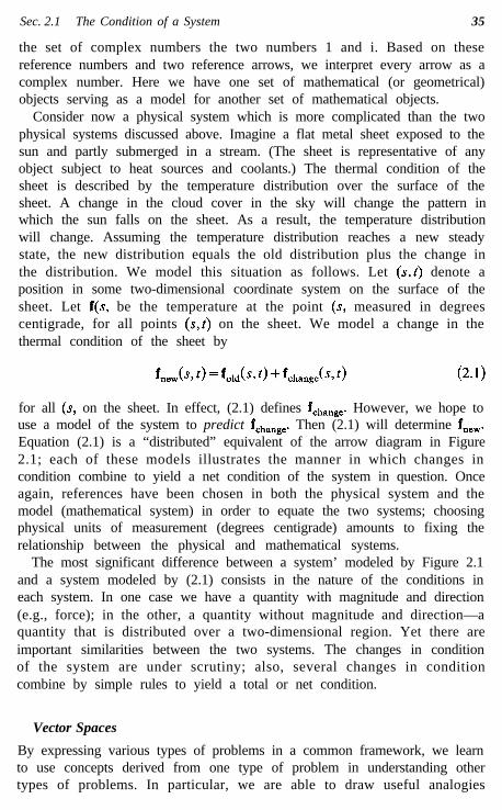
Consider now a physical system which is more complicated than the twophysical systems discussed above. Imagine a flat metal sheet exposed to thesun and partly submerged in a stream. (The sheet is representative of anyobject subject to heat sources and coolants.) The thermal condition of thesheet is described by the temperature distribution over the surface of thesheet. A change in the cloud cover in the sky will change the pattern inwhich the sun falls on the sheet. As a result, the temperature distributionwill change. Assuming the temperature distribution reaches a new steadystate, the new distribution equals the old distribution plus the change inthe distribution. We model this situation as follows. Let (s,t) denote aposition in some two-dimensional coordinate system on the surface of thesheet. Let f(s,t) be the temperature at the point (s,t), measured in degreescentigrade, for all points (s,t) on the sheet. We model a change in thethermal condition of the sheet by
(2.1)
for all (s,t) on the sheet. In effect, (2.1) defines fchange. However, we hope touse a model of the system to predict fchange. Then (2.1) will determine fnew.Equation (2.1) is a “distributed” equivalent of the arrow diagram in Figure2.1; each of these models illustrates the manner in which changes incondition combine to yield a net condition of the system in question. Onceagain, references have been chosen in both the physical system and themodel (mathematical system) in order to equate the two systems; choosingphysical units of measurement (degrees centigrade) amounts to fixing therelationship between the physical and mathematical systems.
The most significant difference between a system’ modeled by Figure 2.1and a system modeled by (2.1) consists in the nature of the conditions ineach system. In one case we have a quantity with magnitude and direction(e.g., force); in the other, a quantity without magnitude and direction—aquantity that is distributed over a two-dimensional region. Yet there areimportant similarities between the two systems. The changes in conditionof the system are under scrutiny; also, several changes in conditioncombine by simple rules to yield a total or net condition.
Vector Spaces
By expressing various types of problems in a common framework, we learnto use concepts derived from one type of problem in understanding othertypes of problems. In particular, we are able to draw useful analogies

36 System Models: Transformations on Vector Spaces
between algebraic equations and differential equations by expressing bothtypes of equations as “vector” equations. Therefore, we now generalize thecommon notion of a vector to include all the examples discussed in theprevious section.
Definition. A linear space (or vector space) v is a set of elements x, y,Z,***, called vectors, together with definitions of vector addition and scalarmultiplication.
a. The definition of vector addition is such that:1. To every pair, x and y, of vectors in V there corresponds a
unique vector x+ y in “/, called the sum of x and y.2 . x+y=y+x.3 . (x+y)+z=x+(y+z).4. There is a unique vector 8 in ?r, called the zero vector (or
origin), such that x + 8 =x for all x in ‘V.5. Corresponding to each x in 7/ there is a unique vector “-x” in
Ir such that x+(-x)[email protected]. The definition of scalar multiplication is such that:
1. To every vector x in ?r and every scalar a there corresponds aunique vector ax in Y, called the scalar multiple of x?
2. a(bx) = (ab)x.3 . l(x) =x (where 1 is the unit scalar).4 . a(x+y)=ax+ ay.5 . (a+b)x=ax+ bx.
Notice that a vector space includes not only a set of elements (vectors)but also “valid” definitions of vector addition and scalar multiplication.Also inherent in the definition is the fact that the vector space Ir containsall “combinations” of its own vectors: if x and y are in V, then ax+ by isalso in ?r. The rules of algebra are so much a part of us that some of therequirements may at first appear above definition; however, they arenecessary. A few more vector space properties which may be deduced fromthe above definition are as follows:
1. Ox= 8 (where “0” is the zero scalar).2. d9= 8.3. (- 1)x= -xx.
Example 1. The Real 3-tuple Space S3. The space 9’ consists in the set of all
*The scalars are any set of elements which obey the usual rules of algebra. A set of elementswhich obeys these rules constitutes a field (see Hoffman and Kunze [2.6]). We usually use asscalars either the real numbers or the complex numbers. There are other useful fields, however(P&C 2.4).

Sec. 2.1 The Condition of a System 37
real 3- tuples (al l ordered sequences of three real numbers) , x = (&,&,Q, y= (~i,r)~,~), with the following definitions of addition and scalar multiplication:
(2.2)
It is clear that the zero vector for this 3-tuple space, 8 = (0,0,0), satisfies x + 8 =x.We show that 0 is unique by assuming another vector y also satisfies x+ y =x; thatis,
or & + 7jj = &. The properties of scalars then require vi=0 (or y = e). It is easy toprove that 9L3, as defined above, satisfies the other requirements for a linear space.In each instance, questions about vectors are reduced to questions about scalars.
We emphasize that the definition of a3 says nothing about coordinates.Coordinates are multipliers for reference vectors (reference arrows, forinstance). The 3-tuples are vectors in their own right. However, there is acommonly used correspondence between $FL3 and the set of vectors (ar-rows) in the usual three-dimensional space which makes it difficult not tothink of the 3-tuples as coordinates. The two sets of vectors are certainlyequivalent. We will, in fact, use this natural correspondence to helpillustrate vector concepts graphically.
Example 2. The Two-Dimensional Space of Points (or Arrows). This space con-sists in the set of all points in a plane. Addition is defined by the parallelogram ruleusing a fixed reference point (see Figure 2.2). Scalar multiplication is defined as“length” multiplication using the reference point. The zero vector is obviously the
Figure 2.2. The two-dimensional space of points.

38 System Models: Transformations on Vector Spaces
reference point. Each of the requirements can be verified by geometrical argu-ments.
An equivalent (but not identical) space is one where the vectors are not thepoints, but rather, arrows to the points from the reference point. We distinguishonly the magnitude and direction of each arrow; two parallel arrows of the samelength are considered identical.
Both the arrow space and the point space are easily visualized: we oftenuse the arrow space in two or three dimensions to demonstrate conceptsgraphically. Although the arrow space contains no inherent referencearrows, we sometimes specify reference arrows in order to equate thearrows to vectors in CJL3. Because of the equivalence between vectors in C9L3and vectors in the three-dimensional space of points, we occasionally referto vectors in $R3 and in other spaces as points.
Example 3. The Space of Column Vectors ‘X3 x ‘. The space 91L3 x ’ consists inthe set of all real 3x1 column matrices (or column vectors), denoted by
with the following definitions of addition and scalar multiplication:
(2.3)
In order to save space in writing, we occasionally write vectors from9lL3x ’ in the transposed form x = (5, t2 t3)‘. The equivalence between9lL3x ’ and 9L3 is obvious. The only difference between the two vectorspaces is in the nature of their vectors. Vectors in 9lL3x ’ can be multipliedby m x 3 matrices (as in Section 1.5), whereas vectors in CR3 cannot.Example 4. The Space of Real Square-Summable Sequences, I,. The space t2consists in the set of all infinite sequences of real numbers, x= ([r,&,t3,. . .),Y=@I~J~,Q,...) which are square summable; that is, for which XF- rti2 < cc.Addition and scalar multiplication in Z, are defined by
ax ii (a&&, 43,. . . )(2.4)
Most of the properties required by the definition of a linear space are easilyverified for Z2; for instance, the zero vector is obviously 8 = (0,0,0, . . .). However,there is one subtle difference between 1, and the space 9L3 of Example 1. Because
Sec. 2.1 The Condition of a System 39
the sequences in Z2 are infinite,in l2. It can be shown that
it is not obvious that if x and y are in I,, x + y is also
[This fact is known as the triangle inequality (P&C 5.4)]. Therefore,
and x + y is square-summable. The requirement of square summability is a definiterestriction on the elements of Z2; the simple sequence (I, 1, 1,. . .), for instance, is notin 12.
The definition of CR3 extends easily to w, the space of n-tuples of realnumbers (where n is a positive integer). The space anx ’ is a similarextension of X3 x ’ Mathematically these “n-dimensional” spaces are no.more complicated than their three-dimensional counterparts. Yet we arenot able to draw arrow-space equivalents because our physical world isthree-dimensional. Visualization of an abstract vector space is most easilyaccomplished by thinking in terms of its three-dimensional counterpart.
The spaces CRn, wx ‘, and I, can also be redefined using complexnumbers, rather than real numbers, for scalars. We denote by $ thecomplex n-tuple space. We use the symbol %zx ’ for the space of complexn x 1 column vectors. Let 1; represent the space of complex square-summable sequences. (We need a slightly different definition of squaresummability for the space Zi:EF= llsi12 < cc). In most vector space defi-nitions, either set of scalars can be used. A notable exception to inter-changeability of scalars is the arrow space in two or three dimensions. Theprimary value of the arrow space is in graphical illustration. We havealready discussed the equivalence of the set of complex scalars to thetwo-dimensional space of arrows. Therefore, substituting complex scalarsin the real two-dimensional arrow space would require four-dimensionalgraphical illustration.
We eventually find it useful to combine simple vector spaces to formmore complicated spaces.
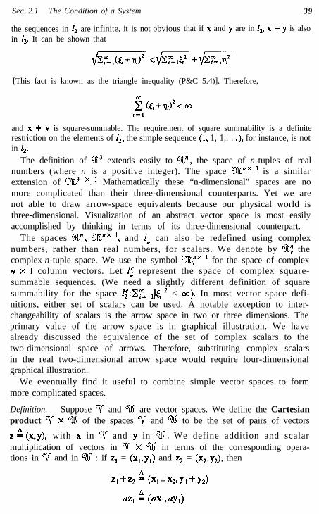
Definition. Suppose ?i and w are vector spaces. We define the Cartesianproduct ?r x 02ui of the spaces Ir and % to be the set of pairs of vectors
z i (X,Y), with x in Ir and y in ‘?.$. We define addition and scalarmultiplication of vectors in Ir x ‘% in terms of the corresponding opera-tions in ‘v and in w : if zr = (x,,y,) and z2 = (x2,y2), then
z,+z, A 0% + x29 Y 1+ Y2)
az, =*(axPaY,)

40 System Models: Transformations on Vector Spaces
Example 5. A Cartesian Product. Let x = (&,t2), a vector in 3’. Let y= (qr), a
vector in 9%‘. Then z i ((51,52), (qi)) is a typical vector in 9L2 x 9’. This Cartesianproduct space is clearly equivalent to 913. Strictly speaking, however, z is not in R3.It is not a 3-tuple, but rather a 2-tuple followed by a 1-tuple. Yet we have no needto distinguish between 913 and %2X 9,‘.
Function Spaces
Each vector in the above examples has discrete elements. It is a smallconceptual step from the notion of an infinite sequence of discrete num-bers (a vector in I,) to the usual notion of a function—a “continuum” ofnumbers. Yet vectors and functions are seldom related in the thinking ofengineers. We will find that vectors and functions can be viewed asessentially equivalent objects; functions can be treated as vectors, andvectors can be treated as functions. A function space is a linear spacewhose elements are functions. We usually think of a function as a rule orgraph which associates with each scalar in its domain a single scalar value.We do not confuse the graph with particular values of the function. Ournotation should also keep this distinction. Let f denote a function; that is,the symbol f recalls to mind a particular rule or graph. Let f(t) denote thevalue of the function at t. By f = g, we mean that the scalars f(t) and g(t) areequal for each t of interest.
Example 6. 9”, The Polynomials of Degree Less Than n. The space 9” consistsin all real-valued polynomial functions of degree less than n : f(t) = & + t2t + - - - +&,t”-’ for all real t. Addition and scalar multiplication of vectors (functions) in qnare defined by
(2.5)
for all t. The zero function is for all t. This zero function is unique; if thefunction g also satisfied f + g=f, then the values of f and g would satisfy
(f+g)(t)=f(t)+g(t)=f(t)
It would follow that for all t, or The other requirements for a vectorspace are easily verified for qp”.
We emphasize that the vector f in Example 6 is the entire portrait of thefunction f. The scalar variable t is a “dummy” variable. The only purposeof this variable is to order the values of the function in precisely the sameway that the subscript i orders the elements in the following vector from Z2:
x=(&t2 ,..., ,,**-5. )
Sec. 2.1 The Condition of a System 41
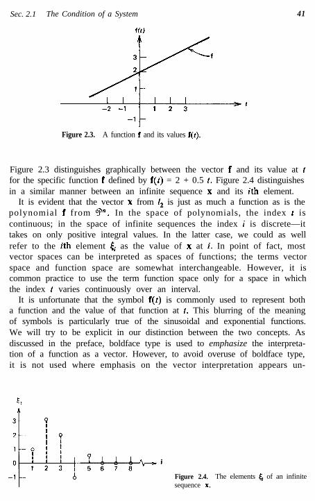
Figure 2.3. A function f and its values f(t).
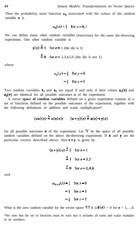
Figure 2.3 distinguishes graphically between the vector f and its value at tfor the specific function f defined by f(t) = 2 + 0.5 t. Figure 2.4 distinguishesin a similar manner between an infinite sequence x and its ith element.
It is evident that the vector x from Z2 is just as much a function as is thepolynomial f from (Tn. In the space of polynomials, the index t iscontinuous; in the space of infinite sequences the index i is discrete—ittakes on only positive integral values. In the latter case, we could as wellrefer to the ith element li as the value of x at i. In point of fact, mostvector spaces can be interpreted as spaces of functions; the terms vectorspace and function space are somewhat interchangeable. However, it iscommon practice to use the term function space only for a space in whichthe index t varies continuously over an interval.
It is unfortunate that the symbol f(t) is commonly used to represent botha function and the value of that function at t. This blurring of the meaningof symbols is particularly true of the sinusoidal and exponential functions.We will try to be explicit in our distinction between the two concepts. Asdiscussed in the preface, boldface type is used to emphasize the interpreta-tion of a function as a vector. However, to avoid overuse of boldface type,it is not used where emphasis on the vector interpretation appears un-
i
Figure 2.4. The elements 6 of an infinitesequence x.

42 System Models: Transformations on Vector Spaces
necessary; thus the value of a function f at t may appear either as f(t) or asf(t). Furthermore, where confusion is unlikely, we sometimes use standardmathematical shorthand; for example, we use Jb,fgdt to mean Jb,f(t)g(t)dt.
It is difficult to describe or discuss functions in any detail except interms of their scalar values. In Example 6, for instance, the definitions ofaddition and scalar multiplication were given in terms of function values.Furthermore, we resorted again to function values to verify that the vectorspace requirements were met. We will find ourselves continually reducingquestions about functions to questions about the scalar values of thosefunctions. Why then do we emphasize the function f rather than the valuef(t)? Because system models act on the whole vector f rather than on itsindividual values. As an example, we turn to the one system model wehave explored thus far-the matrix equation Ax= y which was introducedin Section 1.5. If A is an m X n matrix, the vector x is a column matrix in9lLnX1; y i s in 9Lmx1. Even though the matrix multiplication requiresmanipulation of the individual elements (or values) of x, it is impossible todetermine any element of y without operating on all elements of x. Thus itis natural to think in terms of A operating on the whole vector x. Similarly,equations involving functions require operations on the whole function(e.g., integration), as we shall see in Section 2.3.
Example 7. The Space e(iz, b) of Continuous Functions. T h e v e c t o r s i n e(a,b)are those real functions which are defined and continuous on the intervalAddition and scalar multiplication of functions in (?(a, b) are defined by thestandard function space definitions (2.5) for all t in [a,b]. It is clear that the sumsand scalar multiples of continuous functions are also continuous functions.
Example 8. The Real Square-integrable Functions. The spaceconsists in all real functions which are defined and square integrable on theinterval [a,b]; that is, functions f for which*
/b2f (t)dt<oo
a
Addition and scalar multiplication of functions in are defined by (2.5) forall t in [a,b]. The space lZ,(a,b) is analogous to Z,. It is not clear that the sum oftwo square-integrable functions is itself square integrable. As in Example 4, wemust rely on P&C 5.4 and the concepts of Chapter 5 to find that
*The integral used in the definition of C,(a,b) is the Lebesgue integral. For all practicalpurposes, Lebesgue integration can be considered the same as the usual Riemann integration.Whenever the Riemann integral exists, it yields the same result as the Lebesgue integral. (SeeRoyden [2.l].)

Sec. 2.1 The Condition of a System 43
It follows that if f and g are square integrable, then f + g is square integrable.
Example 9. A Set of Functions. The set of positive real functions [together withthe definitions of addition and scalar multiplication in (2.91 does not form a vectorspace. This set contains a positive valued function f, but not the negative valuedfunction -f; therefore, this set does not include all sums and multiples of itsmembers.
Example 10. Functions of a Complex Variable. Let Y be the space of allcomplex functions w of the complex variable z which are defined and analytic onsome region G! of the complex z plane.* For instance, s1 might be the circle ]z 1 Q 1.We define addition and scalar multiplication of functions in Ir by
(2.6)
for all z in Sk In this example, the zero vector 8 is defined by 8 (z) = 0 for all z in St.(We do not care about the values of the functions 0 and w outside of a.)
Exercise 1. Show that if w1 and w2 are in the space V of Example 10,then w1 + w2 is also in ‘v.
Example 11. A Vector Space of Random Variables t A random variable x is anumerical-valued function whose domain consists in the possible outcomes of anexperiment or phenomenon. Associated with the experiment is a probabilitydistribution. Therefore, there is a probability distribution associated with the valuesof the random variable. For example, the throwing of a single die is an experiment.We define the random variable x in terms of the possible outcomes u by
= 2,4,6 (the die is even)
= 1,3,5 (the die is odd)
The probability mass function w associated with the outcome (I of the experiment isgiven by
*Express the complex variable t in the form s+ it, where s and t are real. Let the complexfunction w be written as u+ iv, where u(z) and v(z) are real. Then w is analytic in !G? if andonly if the partial derivatives of II and v are continuous and satisfy the Cauchy-Riemannconditions in Sz:
For instance, w(z) A z2 is analytic in the whole z plane. See Wylie [2.11].† See Papoulis [2.7], or Cramér and Leadbetter [2.2].
44 System Models: Transformations on Vector Spaces
Then the probability mass function w, associated with the values of the randomvariable x is
o,(x) = 4 forx=O,l
We can define many other random variablesexperiment. One other random variable is
(functions) for the same die-throwing
1 (the die is 1)
2,3,4,5,6 (the die is not 1)
where
Oy(Y) =$ fory=O
=i fory=l
Two random variables x1 and x2 are equal if and only if their values x,(u) andx2(u) are identical for all possible outcomes u of the experiment.
A vector space of random variables defined on a given experiment consists in aset of functions defined on the possible outcomes of the experiment, together withthe following definitions of addition and scalar multiplication*:
for all possible outcomes u of the experiment. Let Y be the space of all possiblerandom variables defined on the above die-throwing experiment. If x and y are theparticular vectors described above, then is given by
and
What is the zero random variable for the vector space Y? It is = 0 for = 1,…,6.
*We note that the set of functions must be such that it includes all sums and scalar multiplesof its members.

Sec. 2.2 Relations Among Vectors 45
2.2 Relations Among Vectors
Combining Vectors
Assuming a vector represents the condition or change in condition of asystem, we can use the definitions of addition and scalar multiplication ofvectors to find the net result of several successive changes in condition ofthe system.
Definition. A vector x is said to be a linear combination of the vectors x,,x29 - * ’ , x, if it can be expressed as
(2.7)
for some set of scalars ci, . . . , cn. This concept is illustrated in Figure 2.5where x= fxi +x2-xX,.
A vector space ‘Y is simply a set of elements and a definition of linearcombination (addition and scalar multiplication); the space V includes alllinear combinations of its own elements. If S is a subset of ?r, the set ofall linear combinations of vectors from S , using the same definition oflinear combination, is also a vector space. We call it a subspace of V. Aline or plane through the origin of the three-dimensional arrow space is anexample of a subspace.
Definition. A subset % of a linear space y is a linear subspace (or linearmanifold) of V if along with every pair, x, and x2, of vectors in %, everylinear combination cix, + czx2 is also in % .* We call ‘% a proper subspaceif it is smaller than Ir; that is if % is not V itself.
Figure 2.5. A linear combination of arrows.
*In the discussion of infinite-dimensional Hilbert spaces (Section 5.3), we distinguish betweena linear subspace and a linear manifold. Linear manifold is the correct term to use in thisdefinition. Yet because a finite-dimensional linear manifold is a linear subspace as well, weemphasize the physically motivated term subspace.

46 System Models: Transformations on Vector Spaces
Example 1. A Linear Subspace. The set of vectors from a3 which are of theform (Cl, $9 cr + ~2) forms a subspace of ?k3. It is, in fact, the set of all linearcombinations of the two vectors (1, 0, 1) and (0, 1, 1).
Example 2. A Solution Space. The set QJ of all solutions to the matrix equation
is a subspace of 32,3x I. By elimination (Section 1.5), we find that %J contains allvectors of the form (0 t2 -t2)=. Clearly, % consists in all linear combinations ofthe single vector (0 1 -l)T. This example extends to general matrices. Let A be anm x n matrix. Let x be in %“x ‘. Using the rules of matrix multiplication (Appen-dix 1) it can be shown that if x1 and x2 are solutions to Ax- 8, then an arbitrarylinear combination crxt + c2x2 is also a solution. Thus the space of solutions is asubspace of 31t” x ‘.
Example 3. Subspaces (Linear Manifolds) of Functions. Let (.?2(s2) be the space ofall real-valued functions which are defined and have continuous second partialderivatives in the two-dimensional region Sk (This region could be the square0 Q s < 1,O < t < 1, for instance.) Let r denote the boundary of the region Qt. Linearcombination in e’(s2) is defined by
(f+g)W i f(s,t)+gb,t)
(afh 0 9 df(s, 0)(2.8)
for all (s, t) in !Z The functions f in (Z’(G) which satisfy the homogeneous boundarycondition f(s, t) = 0 for (s, t) on I? constitute a linear manifold of e2(Q). For if f, andf, satisfy the boundary condition, then (ctf, + c2fz)(s, t) = crf,(s, t) + czf2(s, t) = 0,and the arbitrary linear combination ctfr + c2f2 also satisfies the boundary condi-tion.
The set of solutions to Laplace’s equation,
(2.9)
for all (s, t) in !J, also forms a linear manifold of c’(s2). For if f, and f2 both satisfy(2.9), then
a 2klfl(s, t) + czus, 01 + a 2[Clf,(s,t) + c2f2(s, 01 = o
as2 at2
and the arbitrary linear combination crf, + c2f2 also satisfies (2.9). Equation (2.9) isphrased in terms of the values of f. Laplace’s equation can also be expressed in the

Sec. 2.2 Relations Among Vectors 47
vector notation
V2f=0 (2.10)
The domain of definition &? is implicit in (2.10). The vector 8 is defined by8 (s, t) = 0 for all (s, t) in a.
In using vector diagrams to analyze physical problems, we often resolvea vector into a linear combination of component vectors. We usually dothis in a unique manner. In Figure 2.5, x is not a unique linear combina-tion of xi, x2, and x3; x = Ox, +3x,+ 2x, is a second resolution of x; thenumber of possible resolutions is infinite. In point of fact, x can berepresented as a linear combination of any two of the other vectors; thethree vectors xi, x2, and x3 are redundant as far as representation of x isconcerned.
Definition. The vectors xi, x2,. . . , x,, are linearly dependent (or coplanar) ifat least one of them can be written as a linear combination of the others.Otherwise they are linearly independent. (We often refer to sets of vectorsas simply “dependent” or “independent.“)
In Figure 2.5 the set {xi, x2, x3} is dependent. Any two of the vectorsform an independent set. In any vector space, a set which contains the 8vector is dependent, for 8 can be written as zero times any other vector inthe set. We define the 8 vector by itself as a dependent set.
The following statement is equivalent to the above definition of inde-pendence: the vectors xi, x2,. . . , x, are linearly independent if and only if
c,x,+c2x2+- +c,x,=e * c1=*** =cn=o (2.11)
Equation (2.11) says the “zero combination” is the only combination thatequals 8. For if ci were not 0, we could simply divide by Ci to find Xi as alinear combination of the other vectors, and the set (xi> would bedependent. If ci = 0, Xi cannot be a linear combination of the other vectors.Equation (2.11) is a practical tool for determining independence of vectors.
Exercise 1. Explore graphically and by means of (2.11) the following setof vectors from
Example 4. Determining Independence In the space (X3 let xl = (1, 2, l), x2 = (2,3, l), and x3 = (4, 7, 3). Equation (2.11) becomes

48 System Models: Transformations on Vector Spaces
Each component of this vector equation is a scalar-valued linear algebraic equa-tion. We write the three equations in the matrix form:
We solve this equation by elimination (Section 1.5) to find cl = - 2c, and c2 = - c3.Any choice for c3 will yield a particular nonzero linear combination of the vectorsx1, x2, x3 which equals 8. The set is linearly dependent.
Definition. Let s e {xi, x2,. . . ,x,,} be a set of vectors from a linear spaceV. The set of all linear combinations of vectors from S is called thesubspace of Y spanned (or generated) by 5 .* We often refer to thissubspace as span( S ) or span
Bases and Coordinates
We have introduced the vector space concept in order to provide acommon mathematical framework for different types of systems. We canmake the similarities between systems more apparent by converting theirvector space representations to a standard form. We perform this stan-dardization by introducing coordinate systems. In the example of Figure2.5, the vectors {x, xi, x2, x3} span a plane; yet any two of them will spanthe same plane. Two of them are redundant as far as generation of theplane is concerned.
Definition. A basis (or coordinate system) for a linear space ?r is alinearly independent set of vectors from ?r which spans Ir.
Example 5. The Standard Bases for $Iln, OJR” x ‘, and 9”. It is evident that anythree linearly independent vectors in S3 form a basis for CR3. The n-tuples
(2.12)
form a basis for 9’. The set E i {et,...,e,} is called the standard basis for 9Ln.
We use the same notation to represent the standard basis for
where e, is a column vector of zeros except for a 1 in the ith place. The set % i {f,,
f,, * * * , f,} defined by fk(t)= tkT1 forms a basis for 9” ; it is analogous to thestandard bases for 3,” and
*The definition of the space spanned by an infinite set of vectors depends on limitingconcepts. We delay the definition until Section 5.3.
Sec. 2.2 Relations Among Vectors 49
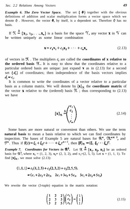
Example 6. The Zero Vector Space. The set { 6} together with the obviousdefinitions of addition and scalar multiplication forms a vector space which wedenote 0 . However, the vector 8, by itself, is a dependent set. Therefore 0 has nobasis.
If !X : {Xi, x2,. . .,x,} is a basis for the space V, any vector x in V canbe written uniquely as some linear combination
x=clxl+czx2+“’ +c,x, (2.13)
of vectors in % . The multipliers ci are called the coordinates of x relative tothe ordered basis %. It is easy to show that the coordinates relative to aparticular ordered basis are unique: just expand x as in (2.13) for a secondset {di} of coordinates; then independence of the basis vectors implies4= ci.
It is common to write the coordinates of a vector relative to a particularbasis as a column matrix. We will denote by [xl% the coordinate matrix ofthe vector x relative to the (ordered) basis % ; thus corresponding to (2.13)we have
(2.14)
Some bases are more natural or convenient than others. We use the termnatural basis to mean a basis relative to which we can find coordinates byinspection. The bases of Example 5 are natural bases for %‘, Xnx i, andCP’. Thus if f(t)=&+t2‘zt+-- +&t”-‘, then [f],=(& 52-$,)T.
Example 7. Coordinates for Vectors in S3. Let OX i {x1, x2, x,} be an orderedbasis for 9t3, where x1 = (1, 2, 3), x2= (2, 3, 2), and x3=(2, 5, 5). Let x = (1, 1, 1). Tofind [xl,, we must solve (2.13):
++2C2+2C3, 2Cl+3C2+5C3, 3C,+2C2+5C3)
We rewrite the vector (3-tuple) equation in the matrix notation:
(2.15)

50 System Models: Transformations on Vector Spaces
We solved this equation in Example 1 of Section 1.5. The result is
The coordinate matrix of Example 7 is merely a simple way of statingthat x= 3x1 +$x2- $,x3. We choose to write the coordinates of a vector xas a column matrix because it allows us to carry out in a standard matrixformat all manipulations involving the coordinates of x.
In Example 4 of Section 1.5 we solved (2.15) with a general right-handside; that is, for x=(~~,r/~,~). That solution allows us to determine quicklythe coordinate matrix, relative to the basis !X of Example 7, for any vectorx in $F13, including the case x= (0, 0, 0). In general, (2.13) includes (2.11);inherent in the process of finding coordinates for an arbitrary vector x isthe process of determining whether 3(, is a basis. If % is not independent,there will exist nonzero coordinates for x= 8. If % does not span thespace, there will be some vector x for which no coordinates exist (P&C2.7).
Example 8. Coordinates for Vectors in 9’. Let S i {f,, f2, f,} be an orderedbasis for q3, where f,(t)= 1 +2t+3t2, f2(t)=2+3t+2t2, and f3(t)=2+5t+5t2. Letf be defined by f(t) = 1 + t + t2. To find [f],, we solve (2.13), f = c,f l + c2f2 + c3f3. Tosolve this equation, we evaluate both sides at t:
f(t) = (c,f1+ c2f2 + c$3)(0
= Clf,(d + &W + @3(t) (2.16)
1+t+t2=c1(1+2t+3t2)+c2(2+3t+2t2)+c3(2+5t+5t2)
Equating coefficients on like powers of t we again obtain (2.15). The coordinatematrix of f is
In order to solve the vector (function) equation (2.16) we converted it toa set of scalar equations expressed in matrix form. A second method for

Sec. 2.2 Relations Among Vectors 51
converting (2.16) to a matrix equation in the unknowns {c,.} is to evaluatethe equation at three different values of t. Each such evaluation yields analgebraic equation in { ci}. The resulting matrix equation is different from(2.15), but the solution is the same. We now describe a general method,built around a natural basis, for converting (2.13) to a matrix equation. Thecoordinate matrix of a vector x relative to the basis !?C = {x1,. . . , xn} isCxln = (c, - * * CJ’, where the coordinates ci are obtained by solving thevector equation
x=c,x,+-*- +c,x,
A general method for obtaining an equivalent matrix equation consists intaking coordinates of the vector equation relative to a natural basis —abasis relative to which coordinates can be obtained by inspection. Thevector equation becomes
(2.17)
We determine [xl%, [x&, … , [x,]~ by inspection. Then we solve (2.17)routinely for [xl%.
Example 9. Finding Coordinates via a Natural Basis. Let the set 9 2 {f,, f,, f3}
be a basis for 9’, where f,(t)=l+2t+3t2, f2(t)=2+3t+2t2, and f,(t)=2+5t+5 t2. We seek [f], for the vector f(t) = 1 + t + t2. To convert the defining equation forcoordinates into a matrix equation, we use the natural basis CJC i {gl, g2, g3},where gk(t)= t k-1. For this problem, (2.17) becomes
VI, = (PII, :. P21, i [r,l,)mT
or
The solution to this equation is [f], = (5 $ - 3)‘. (Compare with Example 8.)

52 System Models: Transformations on Vector Spaces
Typically, the solution of (2.17) requires the elimination procedure
(2.18)
If we wish to solve for the coordinates of more than one vector, we stillperform the elimination indicated in (2.18), but augment the matrix withall the vectors whose coordinates we desire. Thus if we wish thecoordinates for zi, z2, and z3, we perform elimination on
This elimination requires less computation than does the process whichgoes through inversion of the matrix ([xi]% i l - l i [x,,]~), regardless ofthe number of vectors whose coordinates we desire (P&C 1.3).
Example 10. A Basis and Coordinates for a Subspace. Let %! be the subspace ofTp3 consisting in all functions f defined by the rule f(t)=& + t2t + (& +&)t2 forsome [i and t2. Note that the standard basis functions for Y3 are not contained in‘?lf. The functions defined by gi( t) = 1 + t2 and g2(t) = t + t2 are clearly independentvectors in %. Because there are two “degrees of freedom” in % (i.e., twoparameters [i and 42 must be given to specify a particular function in 7JJ) we
expect the set 9 4 {gi, g2} to span %f and thus be a basis. We seek the coordinatematrix [f], of an arbitrary vector f in ‘%f . That is, we seek cl and c2 such that
f(t) = c&(t) + c2g2w
The matrix equation (2.17) can be written by inspection using the natural basis FYZof Example 9:
[II, = ([&I, i k¶2la)Me ~
Then Ci =& and
lfl(1
9 =(6 12
Because we were able to solve uniquely for the coordinates, we know that4 is indeed a basis for %. The subspace % is equivalent to the subspaceof Example 1. Note that the elimination procedure does not agree precisely

Sec. 2.2 Relations Among Vectors 53
with (2.18) because there are only two degrees of freedom among the threecoefficients of the arbitrary vector f in W .
Dimension
The equivalence between the three vector spaces CR3, T3, and 9lL3x ’ isapparent from Examples 7 and 8; The subspace % of Example 10,however, is equivalent to 9R,2x ’ rather than 9L3 x I, even though theelements of % are polynomials in (Y3. The key to the equivalence lies notin the nature of the elements, but rather in the number of “degrees offreedom” in each space (the number of scalars which must be specified inorder to specify a vector); more to the point, the key lies in the number ofvectors in a basis for each space.
Definition. A vector space is finite dimensional if it is spanned by a finitenumber of vectors. It is intuitively clear that all bases for a finite-dimensional space contain the same number of vectors. The number ofvectors in a basis for a finite-dimensional space Y is called the dimensionof ?r and is denoted by dim( ‘Y).
Thus CR3 and 53” are both three-dimensional spaces. The subspace % ofExample 10 has dimension 2. Knowledge of the dimension of a space (or asubspace) is obtained in the course of determining a basis for the space
(subspace). Since the space 0 2 { 8} has no basis, we assign it dimensionzero.
Example 11. A Basis for a Space of Random Variables. A vector space Y ofrandom variables, defined on the possible outcomes of a single die-throwingexperiment, is described in Example 11 of Section 2.1. A natural basis for ‘v is the
set of random variables 5% 9 {Xi, i= 1,...,6}, where
Xi(U) ’ 1 for u = i (the die equals i)
i 0 for (I # i (the die does not equal i)
That 5% is a basis for Y can be seen from an attempt to determine the coordinateswith respect to 5X of an arbitrary random variable z defined on the experiment. If
then [z]% = (ci . . . C6)T; a unique representation exists.

54 System Models: Transformations on Vector Spaces
The random variables {xi,. . . , xg} are linearly independent. However, they arenot statistically independent. Statistical independence of two random variables xand y means that knowledge of the value of one variable, say, x, does not tell usanything about the outcome of the experiment which determines the value of theother variable y, and therefore it tells us nothing about the value of y. The randomvariables {Xi} are related by the underlying die-throwing experiment. If we knowxi = 0, for instance, then we know u # 1 (the die is not equal to 1); the probabilitymass functions for x2,..., x, and for all other vectors in V are modified by theinformation concerning the value of xi. The new probability mass functions for xand y of Example 11, Section 2.1, given that xi = 0, are
ox(x;x,=O) = 5 for x=0 w,(y;x,=O)=l fory=O
=32 forx=l =0 fory=l
The space I2 of square-summable sequences described in Example 4 ofSection 2.1 is obviously infinite dimensional. A direct extension of thestandard basis for % seems likely to be a basis for Z2. It is commonknowledge that functions f in e(O, 27~), the space of functions continuouson [0, 27~1, can be expanded uniquely in a Fourier series of the formf(O=b,+X~., ( ak sinkt + b,cos kt). This fact leads us to suspect that theset of functions
9: (l,sint,cost,sin2t,cos2t,...} (2.19)
forms a basis for L?(O, 2w), and that the coordinates of f relative to thisbasis are
This suspicion is correct. The coordinates (or Fourier coefficients) actuallyconstitute a vector in Z2. We show in Example 11 of Section 5.3 that Z2serves as a convenient standard space of coordinate vectors for infinite-dimensional spaces; in that sense, it plays the same role that %’ x ’ doesfor n-dimensional spaces. Unfortunately, the concepts of independence,spanning sets, and bases do not extend easily to infinite-dimensional vectorspaces. The concept of linear combination applies only to the combinationof a finite number of vectors. We cannot add an infinite number of vectorswithout the concept of a limit; this concept is introduced in Chapter 5.Hence detailed examination of infinite-dimensional function spaces is leftfor that chapter.

Sec. 2.3 System Models 55
There is no inherent basis in any space-one basis is as good as another.Yet a space may have one basis which appears more convenient thanothers. The standard basis for 9” is an example. By picking units ofmeasurement in a physical system (e.g., volts, feet, degrees centigrade) wetie together the system and the model; our choice of units may automati-cally determine convenient or standard basis vectors for the vector spaceof the model (based on, say, 1 V, 1 ft, or 1 O C).
By choosing a basis for a space, we remove the most distinguishingfeature of that space, the nature of its elements, and thus tie each vector inthe space to a unique coordinate matrix. Because of this unique connectionwhich a basis establishes between the elements of a particular vector spaceand the elements of the corresponding space of coordinate matrices, we areable to carry out most vector manipulations in terms of coordinatematrices which represent the vectors. We have selected %,‘x ‘, rather than%“, as our standard n-dimensional space because matrix operations areclosely tied to computer algorithms for solving linear algebraic equations(Section 1.5). Most vector space manipulations lead eventually to suchequations.
Because coordinate matrices are themselves vectors in a vector space(w x ‘), we must be careful to distinguish vectors from their coordinates.The confusion is typified by the problem of finding the coordinate matrixof a vector x from wx ’ relative to the standard basis for ntnx ‘. In thisinstance [xl, =x; the difference between the vector and its coordinatematrix is only conceptual. A vector is simply one of a set of elements,although we may use it to represent the physical condition of some system.The coordinate matrix of the vector, on the other hand, is the unique set ofmultipliers which specifies the vector as a linear combination of arbitrarilychosen basis vectors.
2.3 System Models
The concept of a vector as a model for the condition or change incondition of a system is explored in Sections 2.1 and 2.2. We usuallyseparate the variables which pertain to the condition of the system into twobroad sets: the independent (or input) variables, the values of which aredetermined outside of the system, and the dependent (or output) variables,whose values are determined by the system together with the independentvariables. A model for the system itself consists in expressions of relationsamong the variables. In this section we identify properties of systemmodels.

56 System Models: Transformations on Vector Spaces
Example I. An Economic System Let x represent a set of inputs to the U. S.national economy (tax rates, interest rates, reinvestment policies, etc.); let yrepresent a set of economic indicators (cost of living, unemployment rate, growthrate, etc.). The system model T must describe the economic laws which relate y toX.
Example 2. A Baking Process. Suppose x is the weight of a sample of claybefore a baking process and y is the weight after baking. Then the system model Tmust describe the chemical and thermodynamic laws insofar as they relate x and y.
Example 3. A Positioning System. Suppose the system of interest is an armature-controlled motor which is used to position a piece of equipment. Let x representthe armature voltage, a function of time; let y be the shaft position, anotherfunction of time. The system model T should describe the manner in which thedynamic system relates the function y to the function x.
The variables in the economic system of Example 1 clearly separate intoinput (or independent) variables and output (or system condition)variables. In Example 2, both the independent and dependent variablesdescribe the condition of the system. Yet we can view the condition beforebaking as the input to the system and view the condition after baking asthe output. The dynamic system of Example 3 is reciprocal; x and y aremutually related by T. Since the system is used as a motor, we view thearmature voltage x as the input to the system and the shaft position y asthe output. We could, as well, use the machine as a dc generator; then wewould view the shaft position as the input and the armature voltage as theoutput.
The notation TX = y that we introduced in (1.1) implies that the model Tdoes something to the vector x to yield the vector y. As a result, we mayfeel inclined to call x the input and y the output. Yet in Section 1.3 we notethat equations are sometimes expressed in an inverse form. The positionsof the variables in an equation do not determine whether they are inde-pendent or dependent variables. Furthermore, we can see from Example 3that the input and output of a system in some instances may be determinedarbitrarily. In general, we treat one of the vectors in the equation TX = y asthe input and the other as the output. However, unless we are exploring aproblem for which the input is clearly defined, we use the terms input andoutput loosely in reference to the known and unknown variables, respec-tively.
Transformations on Vector Spaces
Our present purpose is to make more precise the vaguely defined model Tintroduced in (1.1) and illustrated above.
Definition. A transformation or function T: 5 ,-) s, is a rule that

Sec. 2.3 System Models 57
associates with each element of the set S, a unique element from the setS,*. The set S, is called the domain of T; 5, is the range of definition of T.
Our attention is directed primarily toward transformations where s, andS, are linear spaces. We speak of T: V+ (?l! as a transformation from thevector space ‘v into the vector space W. An operator is another term for atransformation between vector spaces. We use this term primarily whenthe domain and range of definition are identical; we speak of T: V+ ?r asan operator on V. If S y is a subset of ?r, we denote by T( s y) the set ofall vectors TX in % for which x is in s y; we refer to T( S y) as the imageof S y under T. The range of T is T(V), the image of V under T. Thenullspace of T is the set of all vectors x in V such that TX = 8, (8, is thezero vector in the space %). If SW is a subset of ‘?&, we call the set ofvectors x in Ir for which TX is in S U the inverse image of S GuT. Thus thenullspace of T is the inverse image of the set { 8, }. See Figure 2.6.
Figure 2.6. Abstract illustration of a transformation T.
Example 4. A Transformation Define T: ?iL2+%’ by
T(L52) :)/G-l for(f+<i>l (2.20)
AO= for [f+[i< 1
Physically, the vector TX can be interpreted as the distance between x and the unitcircle in the two-dimensional arrow space. The variables t, and I2 are “dummy”variables; they merely assist us in cataloguing the “values” of T in the defining
*In the modeling process we use the function concept twice: once as a vector—a model forthe condition of a system—and once as a relation between input and output vectors—a modelfor the system itself. In order to avoid confusion, we use the term function in referring tovectors in a vector space, but the term transformation in referring to the relation betweenvectors.
58 System Models: Transformations on Vector Spaces
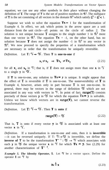
equation; we can use any other symbols in their place without changing thedefinition of T. The range of T is the set of positive numbers in al. The nullspaceof T is the set consisting of all vectors in the domain R2 which satisfy [f + 6,’ < 1.
Suppose we wish to solve the equation TX= 1 for the transformation ofExample 4. In effect, we ask which points in the arrow space are a unitdistance from the unit circle—all points on the circle of radius 2. Thesolution is not unique because T assigns to the single number 1 in 3’ morethan one vector in S2. The equation TX = -1, on the other hand, has nosolution because T does not assign the number -1 in %’ to any vector inCF12. We now proceed to specify the properties of a transformation whichare necessary in order that the transformation be uniquely reversible.
Definition. Let T: ?r+ “?ti. Then T is one-to-one if
Xl 7-2 + TX, #TX, (2.21)
for all x, and x2 in 1/; that is, if T does not assign more than one x in ?rto a single y in %J.
If T is one-to-one, any solution to TX= y is unique. It might appear thatthe effect of T is reversible if T is one-to-one. The nonreversibility of T inExample 4, however, arises only in part because T is not one-to-one. Ingeneral, there may be vectors in the range of definition % which are notassociated in any way with vectors in Ir. In point of fact, range(T) consistsprecisely of those vectors y in w for which the equation TX= y is solvable.Unless we know which vectors are in range(T), we cannot reverse thetransformation.
Definition. Let T: V+ %. Then T is onto if
range(T) = % (2.22)
That is, T is onto if every vector y in ‘% is associated with at least onevector x in V.
Definition. If a transformation is one-to-one and onto, then it is invertible—it can be reversed uniquely. If T: ‘v+(% is invertible, we define theinverse of T to be the transformation T- ’ : w + Y which associates witheach y in % the unique vector x in V for which TX = y. See (2.29) foranother characterization of T- ‘.
Example 5. The Identity Operator, I. Let V be a vector space. Define theoperator I on Y by
IX:, (2.23)

Sec. 2.3 System Models 59
for all x in Y. The nullspace of I is &. Range (I)= ?r; thus I is onto. Furthermore,I is one-to-one. Therefore, the identity operator is invertible.
Example 6. The Zero Transformation, 8. Let Y and % be vector spaces. Define9: T’-+%J b y
e&ew (2.24)
for all x in Y. The nullspace of 8 is Y. The range of 8 is eW. The zerotransformation is neither one-to-one nor onto. It is clearly not invertible.
Example 7. A Transformation on a Function Space. Define T: b? (a,b)+%,’ by
Tf k lbff2(t)dta
(2.25)
for all f in (2 (a, b). This transformation specifies an integral-square measure of thesize of the function f; this measure is used often in judging the performance of acontrol system. The function f is a dummy variable used to define T; the scalar t isa dummy variable used to define f. In order to avoid confusion, we must carefullydistinguish between the concept of the function f in the vector space e(a, b) andthe concept of the transformation T which relates each function f in (?(a, 6) to avector in 9%‘. The transformation acts on the whole function f-we must use allvalues of f to find Tf. The range of T is the set of positive numbers in a’; thus T isnot onto the range of definition CFL’. The nullspace of T is the single vector fIy. Ifwe define f, and f2 by f,(t) = 1 and f2(t) = -1, then Tf, = Tf2; therefore T is notone-to-one.
The transformations of Examples 4 and 7 are scalar valued; that is, therange of definition in each case is the space of scalars. We call ascalar-valued transformation a functional. Most functionals are not one-to-one.
Example 8. A Transformation for a Dynamic System. Let e2(a, b) be the space offunctions which have continuous second derivatives on .[a, b]. Define L: e2(a, b)+WO) by
(Lf)(t) e f~(t)+,(f(t)+0.01f3(t>) (2.26)
for all f in lZ2(a, b) and all t in [a, b]. This transformation is a model for a particularmass-spring system in which the spring is nonlinear. The comments under Example7 concerning the dummy variables f and t apply here as well. As usual, thedefinition is given in terms of scalars, functions evaluated at t. Again, L acts on thewhole function f. Even in this example we cannot determine any value of thefunction Lf without using an “interval” of values of f, because the derivative

60 System Models: Transformations on Vector Spaces
function f’ is defined in terms of a limit of values of f in the neighborhood of t:
The nullspace of L consists in all solutions of the nonlinear differential equation,Lf-eW ; restated in terms of the values of Lf, this equation is
f”(t)+a(f(t)+0.01f3(t))=0 a<t<b
To determine these solutions is not a simple task. By selecting C? (a, b) as the rangeof definition, we ask that the function Lf be continuous; since Lf represents a forcein the mass-spring system described by (2.26) continuity seems a practical assump-tion. By choosing e’(a,b) as the domain, we guarantee that Lf is continuous. Yetthe range of L is not clear. It is in the range of definition, but is it equal to therange of definition? In other words, can we solve the nonlinear differentialequation Lf =u for any continuous u? The function f represents the displacementversus time in the physical mass-spring system. The function u represents the forceapplied to the system as a function of time. Physical intuition leads us to believethat for given initial conditions there is a unique displacement pattern f associatedwith each continuous forcing pattern u. Therefore, L should be onto. On the otherhand, since no initial conditions are specified, we expect two degrees of freedom inthe solution to Lf =u for each continuous u. Thus the dimension of nullspace (L) istwo, and L is not one-to-one.
Combining Transformations
The transformation introduced in Example 8 is actually a composite ofseveral simpler transformations. In developing a model for a system, weusually start with simple models for portions of the system, and thencombine the parts into the total system model. Suppose T and U are bothtransformations from II into % . We define the transformation aT+ bU:‘-lb% b y
(aT+ bU)x 4 aTx + bUx (2.27)
for all x in V. If G: % +G%, we define the transformation GT: V+%bY
(GT)x i G(Tx) (2.28)
for all x in Ir. Equations (2.27) and (2.28) define linear combination andcomposition of transformations, respectively.

Sec. 2.3 System Models 61
Example 9. Composition of Matrix Multiplications. Define G: a3+a2 by
and T: CR2+CX3 by
$3 i (5 $)
Then GT: (Zk2+CR2 is described by
Exercise 1. Let T: Y+%. Show that T is invertible if and only ifV = % and there is a transformation T- ’ : % -+ Y such that
T-‘T=m-l=I (2.29)
Exercise 2. Suppose G and T of (2.26) are invertible. Show that
(GT)-‘=T-‘G-l (2.30)
The composition (or product) of two transformations has two nastycharacteristics. First, unlike scalars, transformations usually do not com-mute; that is, GT#TG. As illustrated in Example 9, G and T generally donot even act on the same vector space, and TG has no meaning. Even if Gand T both act on the same space, we must not expect commutability, asdemonstrated by the following matrix multiplications:

62 System Models: Transformations on Vector Spaces
Commutable operators do exist. In fact, since any operator commutes withitself, we can write G2, as we do in Example 10 below, without beingambiguous. Operators which commute act much like scalars in theirbehavior toward each other (see P&C 4.29).
If two scalars satisfy ab = 0, then either a = 0, b = 0, or both. The secondmatrix multiplication above demonstrates that this property does notextend even to simple transformations. This second difficulty with thecomposition of transformations is sometimes called the existence of divi-sors of zero. If GT =8 and G #9, we cannot conclude that T = 9 ; thecancellation laws of algebra do not apply to transformations. The difficultylies in the fact that for transformations there is a “gray” region betweenbeing invertible and being zero. The range of T can lie in the nullspace ofG.
Example 10. Linear Combination and Composition of Transformations. Thespace en (a, b) consists in all functions with continuous nth derivatives on [a, b].
Define G: 67” (a, b)+P-‘(a,b) by Gf 9 f’ for all f in en (a, b). Then G2: e2(a, b)
+ e (a, b) is well defined. Let U: CZ2(a, b)+ e(a, 6) be defined by (Uf)(t) i f(t)+ 0.01f3(t) for all f in e2(a, b) and all t in [a, b]. The transformation L of Example 8
can be described by L 9 G2 + au.
As demonstrated by the above examples, the domain and range ofdefinition are essential parts of the definition of a transformation. Thisimportance is emphasized by the notation T: ‘v+w. The spaces li‘ andG2Lci are selected to fit the structure of the situation we wish to model. If wepick a domain that is too large, the operator will not be one-to-one. If wepick a range of definition that is too large, the operator will not be onto.Thus both ‘Y and ‘?lJ affect the invertibility of T. We apply loosely theterm finite (infinite) dimensional transformation to those transformationsthat act on a finite (infinite) dimensional domain.
2.4 Linear Transformations
One of the most common and useful transformations is the matrixmultiplication introduced in Chapter 1. It is well suited for automaticcomputation using a digital computer. Let A be an m X n matrix. Wedefine T: Wx1+9?Yx1 by
TX 5 Ax (2.3 1)
for all x in QYxl. We distinguish carefully between T and A. T is not A,but rather multiplication by A. The nullspace of T is the set of solutions to
Sec. 2.4 Linear Transformations 63
the matrix equation Ax= 8. Even though T and A are conceptuallydifferent, we sometimes refer to the nullspace of T as the nullspace of A.
Similarly, we define range(A) b range(T).Suppose A is square (m = n) and invertible; then the equation TX = Ax
= y has a unique solution x = A- ‘y for each y in W x ‘. But T- ’ is definedas precisely that transformation which associates with each y in W x ’ theunique solution to the equation TX= y. Therefore, T is invertible, and T- ’ :
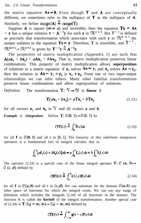
is given by T- ‘y 2 A- ‘y.The properties of matrix multiplication (Appendix 1) are such that
A(ax, + bx,) = aAx, + bAx,. That is, matrix multiplication preserves linearcombinations. This property of matrix multiplication allows superpositionof solutions to a matrix equation: if x1 solves Ax= y, and x2 solves Ax =y2,then the solution to Ax= y, +y2 is x, +x2. From one or two input-outputrelationships we can infer others. Many other familiar transformationspreserve linear combinations and allow superposition of solutions.
Definition. The transformation T: V+G2l(j is linear if
T(ax, + bx2) = aTx, + bTx, (2.32)
for all vectors x1 and x2 in II‘ and all scalars a and b.
Example 1. Integration. Define T: C?(O, l)+(?(O, 1) by
(Tf)(t) A i*f(s)ds (2.33)
for all f in e(O, 1) and all t in [0, I]. The linearity of this indefinite integrationoperation is a fundamental fact of integral calculus; that is,
The operator (2.33) is a special case of the linear integral operator T: C? (a, b)-+(? (c, d) defined by
(2.34)
for all f in e(a,b) and all t in [c,d]. We can substitute for the domain e(a,b) anyother space of functions for which the integral exists. We can use any range ofdefinition which includes the integrals (2.34) of all functions in the domain. Thefunction k is called the kernel of the integral transformation. Another special caseof (2.34) is T: h( - 00, oo)+ h( - co, cc) defined by

64 System Models: Transformations on Vector Spaces
for some g in I.Q - co, oo), all f in C,( - cc, co), and all t in (- co, 00). This T isknown as the convolution of f with the function g. It arises in connection with thesolution of linear constant-coefficient differential equations (Appendix 2).
The integral transformation (2.34) is the analogue for function spacesof the matrix multiplication (2.31). That matrix transformation can be ex-pressed
(Tx)~~ i Ati6 i = l,...,mj- 1
(2.35)
for all vectors x in wx i. The symbol .$ represents the jth element of x;the symbol (TX)i means the ith element of TX. In (2.35) the matrix istreated as a function of two discrete variables, the row variable i and thecolumn variable j. In analogy with the integral transformation, we call thematrix multiplication [as viewed in the form of (2.35)] a summationtransformation; we refer to the function A (with values A& as the kernel ofthe summation transformation.
Example 2. Differentiation Define D: @(a, b)+e (a, b) by
(Df)(t) i f’(t) i limf(t+At)-f(t)
At+0dt (2.36)
for all f in @(a,b) and all t in [a,b]; f’(t) is the slope of the graph of f at t; f’ (orDf) is the whole “slope” function. We also use the symbols i and r<‘) in place of Df.We can substitute for the above domain and range of definition any pair offunction spaces for which the derivatives of all functions in the domain lie in therange of definition. Thus we could define D on E!(a, b) if we picked a range ofdefinition which contains the appropriate discontinuous functions. The nullspaceof D is span{ l}, where 1 is the function defined by l(t)= 1 for all t in [a,b]. It iswell known that differentiation is linear; D(clf, + czfi) = clDf, + c2Df2.
We can define more general differential operators in terms of (2.36). The generallinear constant-coefficient differential operator L: c3” (a, b)-+ C? (a, b) is defined, forreal scalars { ai}, by
LiDn+aJY-‘+ -.a +a,1 (2.37)
where we have used (2.27) and (2.28) to combine transformations. A variable-coefficient (or “time-varying”) extension of (2.37) is the operator L: E? (a, b)+e(a,b) defined by*
(Lf)(t) : g&)fyt)+g~(t)f(“-‘)(t)+ ” l +g,(t)f(t) (2.37)
*Note that we use boldface print for some of the functions in (2.38) but not for others. Asindicated in the Preface, we use boldface print only to emphasize the vector or transformationinterpretation of an object. We sometimes describe the same function both ways, f and J
Sec. 2.4 Linear Transformations 65
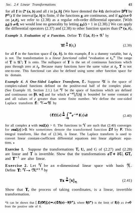
for all f in C?” (a, b) and all t in [a,b]. (We have denoted the kth derivative Dkf byfck).) If the interval [a, b] is finite, if the functions gi are continuous, and if go(t)# 0on [a,b], we refer to (2.38) as a regular n th-order differential operator. [Withgo(t) +O, we would lose no generality by letting go(t) = 1 in (2.38).] We can applythe differential operators (2.37) and (2.38) to other function spaces than (?” (a, 6).
Example 3. Evaluation of a Function. Define T: e(a, b)+ 3’ by
Tf 9 f(t,) (2.39)
for all f in the function space C? (a, b). In this example, f is a dummy variable, butis not. The transformation is a linear functional called “evaluation at t,.” The rangeof T is %,‘; T is onto. The nullspace of T is the set of continuous functions whichpass through zero at t,. Because many functions have the same value at tl, T is notone-to-one. This functional can also be defined using some other function space forits domain.
Example 4. A One-Sided Laplace Transform, t?. Suppose % is the space ofcomplex-valued functions defined on the positive-real half of the complex plane.(See Example 10, Section 2.1.) Let Ir be the space of functions which are definedand continuous on [0, co] and for which e -“‘If(t)1 is bounded for some constant cand all values of t greater than some finite number. We define the one-sidedLaplace transform I?: Y+% by
(ef)(s) i ime-sf f(t)dt (2.40)
for all complex s with real(s) > 0. The functions in Y are such that (2.40) convergesfor real(s)>O. We sometimes denote the transformed function Bf by F. Thisintegral transform, like that of (2.34), is linear. The Laplace transform is used toconvert linear constant-coefficient differential equations into linear algebraic equa-tions. l
Exercise 1. Suppose the transformations T, U, and G of (2.27) and (2.28)are linear and T is invertible. Show that the transformations aT+ bU, GT,and T-l are also linear.
Exercise 2. Let Ir be an n-dimensional linear space with basis 5%.Define T: ‘v-, 9Lnx * by
TX i [xl% (2.41)
Show that T, the process of taking coordinates, is a linear, invertibletransformation.
*It can be shown that [ Ii!(D#Y)(s)-f(O’), where f(O+) is the limit of f(t) as t+Ofrom the positive side of 0.

66 System Models: Transformations on Vector Spaces
The vector space V of Exercise 2 is equivalent to %Yx ’ in every sensewe might wish. The linear, invertible transformation is the key. We say twovector spaces Ir and % are isomorphic (or equivalent) if there exists aninvertible linear transformation from Y into G2K. Each real n-dimensionalvector space is isomorphic to each other real n-dimensional space and,in particular, to the real space w” ‘. A similar statement can be madeusing complex scalars for each space. Infinite-dimensional spaces alsoexhibit isomorphism. In Section 5.3 we show that all well behaved infinite-dimensional spaces are isomorphic to Zz.
Nullpace and Range—Keys to Invertibility
Even linear transformations may have troublesome properties. In point offact, the example in which we demonstrate noncommutability andnoncancellation of products of transformations uses linear transformations(matrix multiplications). Most difficulties with a linear transformation canbe understood through investigation of the range and nullspace of thetransformation.*
Let T: ?f+% be linear. Suppose x,, is a vector in the nullspace of T(any solution to TX= 0); we call xh a homogeneous solution for thetransformation T. Denote by x. a particular solution to the equationTX = y. (An xP exists if and only if y is in range(T).) Then xP + axh is also asolution to TX= y for any scalar (II. One of the most familiar uses of theprinciple of superposition is in obtaining the general solution to a lineardifferential equation by combining particular and homogeneous solutions.The general solution to any linear operator equation can be obtained inthis manner.
Example 5. The General Solution to a Matrix Equation. Define the linear opera-tor T. 9R,2xx+31t2x1 b. Y
Then the equation
Tx=(; :,(;;)=(;)& (2.42)
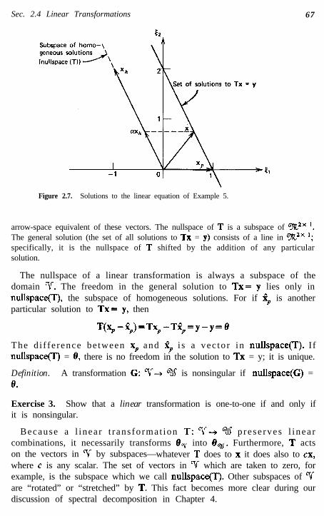
has as its general solution x = ( ). A particular solution is xP = (1 0)T. The2 -2nullspace of T consists in the vector x,, = (-1 2)T and all its multiples. The generalsolution can be expressed as x=xP + ax,, where a is arbitrary. Figure 2.7 shows an
of*See Sections 4.4 and 4.6 for further insight into noncancellation and noncommutabilitylinear operators.
67Sec. 2.4 Linear Transformations
Figure 2.7. Solutions to the linear equation of Example 5.
arrow-space equivalent of these vectors. The nullspace of T is a subspace of 9R,2x *.The general solution (the set of all solutions to TX = y) consists of a line in ‘5X2” ‘;specifically, it is the nullspace of T shifted by the addition of any particularsolution.
The nullspace of a linear transformation is always a subspace of thedomain V. The freedom in the general solution to TX= y lies only innullspace( the subspace of homogeneous solutions. For if 4 is anotherparticular solution to TX= y, then
T@p -$)=Tx,-T$,=y-y=8
The d i f fe rence be tween xP and $ i s a vec to r in nullspace( Ifnullspace = 8, there is no freedom in the solution to TX = y; it is unique.
Definition. A transformation G: v+ % is nonsingular if .nullspace(G) =8.
Exercise 3. Show that a linear transformation is one-to-one if and only ifit is nonsingular.
Because a l inear t r ans format ion T: V+ % prese rves l i nea rcombinations, it necessarily transforms 8, into 8,. Furthermore, T actson the vectors in Y by subspaces—whatever T does to x it does also to cx,where c is any scalar. The set of vectors in ‘Y which are taken to zero, forexample, is the subspace which we call nullspace( Other subspaces of Irare “rotated” or “stretched” by T. This fact becomes more clear during ourdiscussion of spectral decomposition in Chapter 4.

68 System Models: Transformations on Vector Spaces
Example 6. The Action of a Linear Transformation on Subspaces. Define T:
CR3+9L2 by T([,,c2,[3) i (t3,0). The set {xi = (l,O,O), x2=(0, 1,O)) forms a basis fornullspace( By adding a third independent vector, say, x3 = (1, 1, 1), we obtain abasis for the domain 913. The subspace spanned by {xi,x2} is annihilated by T.The subspace spanned by {x3} is transformed by T into a subspace of —therange of T. The vector x3 itself is transformed into a basis for range(T). Because Tacts on the vectors in a3 by subspaces, the dimension of nullspace is a measureof the degree to which T acts like zero; the dimension of range(T) indicates thedegree to which T acts invertible. Specifically, of the three dimensions in a3, Ttakes two to zero. The third dimension of $R3 is taken into the one-dimensionalrange(T).
The characteristics exhibited by Example 6 extend to any linear trans-formation on a finite-dimensional space, Let T: V+% be linear withdim(V) = n. We call the dimension of nullspace the nullity of T. Therank of T is the dimension of rangem. Let {xi,. . . ,xk} be a basis fornullspace( Pick vectors {xk+ r, . . . ,xn} which extend the basis fornullspace to a basis for ‘?f (P&C 2.9). We show that T takes{JQ+p..., x,,} into a basis for range(T). Suppose x= ctx, + l . . + cnxn is anarbitrary vector in ‘v. The linear transformation T annihilates the first kcomponents of x. Only the remaining n-k components are taken intorange(T). Thus the vectors {TX,, ,, . . . ,Tx,} must span range(T). To showthat these vectors are independent, we use the test (2.11):
Since T is linear,
T(&+~JQ+~+.- +5,x,)=@,
Then &+1xk+1+ l . . + 5;1x,, is in nullspace( and
sk+l%+l +**a +&Xn=dlXl+- +dkXk
for some { di}. The independence of {x1,. . . , xn} implies d, = . . . = dk = &+ 1= . . . =&=O; thus {Txk+t,..., TX,} is an independent set and is a basis
for range(T).We have shown that a linear transformation T acting on a finite-
dimensional space V obeys a “conservation of dimension” law:
dim{ v) = rank(T) + nullity(T) (2.43)
Nullity(T) is the “dimension” annihilated by T. Rank(T) is the “dim-ension” T retains. If nullspace = { 8 }, then nullity(T) = 0 and rank(T)= dim(V). If, in addition, dim( %) = dim(V), then rank(T) = dim( ‘?$) (T is

Sec. 2.4 Linear Transformations 69
onto), and T is invertible. A linear T: V+ % cannot be invertible unlessdim(w) = dim( Ir).
We sometimes refer to the vectors xk+ ,, . . . ,x, as progenitors of the rangeof T. Although the nullspace and range of T are unique, the space spannedby the progenitors is not; we can add any vector in nullspace to anyprogenitor without changing the basis for the range (see Example 6).
The Near Nullpace
In contrast to mathematical analysis, mathematical computation is notclear-cut. For example, a set of equations which is mathematicallyinvertible can be so “nearly singular” that the inverse cannot be computedto an acceptable degree of precision. On the other hand, because of thefinite number of significant digits used in the computer, a mathematicallysingular system will be indistinguishable from a “nearly singular” system.The phenomenon merits serious consideration.
The matrix operator of Example 5 is singular. Suppose we modify thematrix slightly to obtain the nonsingular, but “nearly singular” matrixequation
(2.44)
where c is small. Then the arrow space diagram of Figure 2.7 must also bemodified to show a pair of almost parallel lines. (Figure 1.7 of Section 1.5is the arrow space diagram of essentially this pair of equations.) Althoughthe solution (the intersection of the nearly parallel lines) is unique, it isdifficult to compute accurately; the nearly singular equations are very illconditioned. Slight errors in the data and roundoff during computing leadto significant uncertainty in the computed solution, even if the computa-tion is handled carefully (Section 1.5). The uncertain component of thesolution lies essentially in the nullspace of the operator; that is, it is almostparallel to the nearly parallel lines in the arrow-space diagram. The abovepair of nearly singular algebraic equations might represent a nearly singu-lar system. On the other hand, the underlying system might be preciselysingular; the equations in the model of a singular system may be onlynearly singular because of inaccuracies in the data. Regardless of which ofthese interpretations is correct, determining the “near nullspace” of thematrix is an important part of the analysis of the system. If the underlyingsystem is singular, a description of the near nullspace is a description ofthe freedom in the solutions for the system. If the underlying system is justnearly singular, a description of the near nullspace is a description of theuncertainty in the solution.

70 System Models: Transformations on Vector Spaces
Definition. Suppose T is a nearly singular linear operator on a vectorspace v. We use the term near nullspace of T to mean those vectors thatare taken nearly to zero by T; that is, those vectors which T drasticallyreduces in “size.“*
In the two-dimensional example described above, the near nullspaceconsists in vectors which are nearly parallel to the vector x = (-1 2)T. Thenear nullspace of T is not a subspace of ‘v. Rather, it consists in a set ofvectors which are nearly in a subspace of ‘v. We can think of the nearnullspace as a “fuzzy” subspace of ?r.
We now present a method, referred to as inverse iteration, for describingthe near nullspace of a nearly singular operator T acting on a vector spaceV. Let ~0 be an arbitrary vector in Ir. Assume xa contains a componentwhich is in the near nullspace of T. (If it does not, such a component willbe introduced by roundoff during the ensuing computation.) Since Treduces such components drastically, compared to its effect on the othercomponents of ~0, T-’ must drastically emphasize such components.Therefore, if we solve TX, = xa (in effect determining x1 =T- ‘xJ, thecomputed solution xi contains a significant component in the nearnullspace of T. (This component is the error vector which appears duringthe solution of the nearly singular equation.) The inverse iteration methodconsists in iteratively solving Txk+ i =xk. After a few iterations, xk isdominated by its near-nullspace component; we use xk as a partial basisfor the near nullspace of T. (The number of iterations required is at thediscretion of the analyst. We are not looking for a precisely definedsubspace, but rather, a subspace that is fuzzy.) By repeating the aboveprocess for several different starting vectors ~0, we usually obtain a set ofvectors which spans the near nullspace of T.
Example 7. Describing a Near Nullspace. Define a linear operator T on X2” ’by means of the nearly singular matrix multiplication described above:
TX&(: I:r)~
For this simple example we can invert T explicitly
We apply the inverse iteration methodno roundoff in our computations:
to the vector x()=(1 l)=; o f course, we have
x,=( ;), x2= A( yy), x3= -&( “‘;;;;y2),...
*In Section 4.2 we describe the near nullspace more precisely as the eigenspace for thesmallest eigenvalue of T.

Sec. 2.4 Linear Transformations 71
If E is small, say e = 0.01, then
x,=50( f?‘) and ~,=(50)~( -::ii)
After only three iterations, the sequence xk has settled; the vector x3 provides agood description of the near nullspace of T. If E = 0, T is singular; x3 lies almost inthe nullspace of this singular operator (Figure 2.7). Were we to try other startingvectors xe, we would obtain other vectors xk nearly parallel to (-1 2)T. This nearnullspace of T should be considered one-dimensional.
We note from Example 7 that the vector xk in the inverse iteration growsdrastically in size. Practical computer implementations of inverse iterationinclude normalization of xk at each step in order to avoid numbers toolarge for the computer. A description for a two-dimensional near nullspaceis sought in P&C 2.26. In Section 4.2 we analyze the inverse iteration moreprecisely in terms of eigenvalues and eigenvectors. Forsythe [2.3] givessome interesting examples of the treatment of nearly singular operators.
The Role of Linear Transformations
The purpose of modeling a system is to develop insight concerning thesystem, to develop an intuitive feel for the input-output relationship. Inorder to decide whether or not a particular model, linear or nonlinear, is agood model, we must compare the input-output relationship of the modelwith the corresponding, but measurable, input-output relationship of thesystem being modeled. If the model and the system are sufficiently inagreement for our purposes, we need not distinguish between the systemand the model.
Almost all physical systems are to some degree nonlinear. Yet mostsystems act in a nearly linear manner if the range of variation of thevariables is restricted. For example, the current through a resistor isessentially proportional to the applied voltage if the current is not largeenough to heat the resistor significantly. We are able to develop adequatemodels for a wide variety of static and dynamic physical systems usingonly linear transformations. For linear models there is available a vastarray of mathematical results; most mathematical analysis is linear analy-sis. Furthermore, the analysis or optimization of a nonlinear system isusually based on linearization (Chapters 7 and 8). Even in solving anonlinear equation for a given input, we typically must resort to repetitivelinearization.
The examples and exercises of this section have demonstrated thevariety of familiar transformations which are linear: matrix multiplication,differentiation, integration, etc. We introduce other linear transformations

72 System Models: Transformations on Vector Spaces
as we need them. The next few chapters pertain only to linear transforma-tions. In Chapter 3 we focus on the peculiarities of linear differentialsystems. In Chapter 4 we develop the concepts of spectral decompositionof linear systems. The discussion of infinite-dimensional systems inChapter 5 is also directed toward linear systems. Because we use thesymbols T and U so much in reference to linear transformations,hereinafter we employ the symbols F and G to emphasize concepts whichapply as well to nonlinear transformations. We begin to examine nonlinearconcepts in Chapter 6. We do not return fully to the subject of nonlinearsystems, however, until we introduce the concepts of linearization andrepetitive linearization in Chapters 7 and 8.
2.5 Matrices of Linear Transformations
By the process of picking an ordered basis for an n-dimensional vectorspace v, we associate with each vector in v a unique n X 1 columnmatrix. In effect, we convert the vectors in V into an equivalent set ofvectors which are suitable for matrix manipulation and, therefore, auto-matic computation by computer. By taking coordinates, we can alsoconvert a linear equation, TX= y, into a matrix equation. Suppose T:Ir+ % is a linear transformation, dim( ‘V) = n, and dim( %)= m. Pick as
bases for V and (?l! the sets % b {x,, . . . , xn} and 3 i {yl, . . . , y,},respectively. The vectors x in V and TX in % can be represented by theircoordinate matrices [xl, and [TX]%. The vectors x and TX are linearlyrelated (by the linear transformation T). By (2.41), we know that a vectorand its coordinates are also linearly related. Therefore, we expect [xl, and[TX], to be linearly related as well. Furthermore, we intuitively expect thelinear relation between the n x 1 matrix [xl% and the m X 1 matrix [TX]% tobe multiplication by an m x n matrix. We denote this matrix by [T],, andrefer to it as the matrix of T relative to the ordered bases % and 3 ; it mustsatisfy
m&l, i PI, (2.45)
for all x in V. Assume we can find such a matrix. Then by takingcoordinates (with respect to 9 ) of each side of the linear equation TX = y,we convert the equation to the equivalent matrix equation.
[Tl,,[xl, = [Ylcg (2.46)
We will show that we can represent any linear transformation of V into% by a matrix multiplication by selecting bases for ‘V- and —we can

Sec. 2.5 Matrices of Linear Transformations 73
convert any linear equation involving finite-dimensional vector spaces intoa matrix equation. We first show how to determine the matrix of T, thenwe show that it satisfies the defining equation (2.45) for all vectors x in y.
Example 1. Determining the Matrix of a Linear Transformation Let x= (tl, t2,&), an arbitrary vector in 9L3. Define T: 9L3+%2 by
We now find [T],!,G2, where G, and G2 are the standard bases for CR3 and (X2,respectively. By (2.45), we have
for all vectors (&, t2, t3), or
(2.47)
where we have used {au} to represent the elements of [Tj6,6,. By making threeindependent choices of the scalars tr, t2, and t3, we could convert this matrixequation into six equations in the six unknowns {au}. However, by using a littleingenuity, we reduce this effort. Think of the matrix multiplication in terms of thecolumns of [T]63Q2. The ith element of [x]s, multiplies the ith column of [TjQ3Q1. If
we choose x=(1, 0, 0), then [(l, 0, O)],,= i , and (2.47) becomes0
We have found the first column of [TlQ36, directly. We obtain the other twocolumns of [TIQJQz from (2.47) by successive substitution of x= (0, 1, 0) and x=(0,0, 1). The result is
In Example 1 we avoided the need for simultaneous equations bysubstituting the basis vectors ei, e2, and e3 into (2.47) to pick out thecolumns of [T]6,6z. This same technique can be used to find the matrix ofany linear transformation acting on a finite-dimensional space. We referagain to T: V+ ?.$, with dim(V) = n, dim( %) = m, % a basis for v, and9 a basis for %, If we substitute into (2.45) the vector xi, the ith vector of

74 System Models: Transformations on Vector Spaces
the basis % , we pick out the ith column of [T],, :
We can find each column of [T],, independently. The only computa-tional effort is that in determining the coordinate matrices [Txi]%. There-fore,
[Tlaou = ([TX,], : [TX,], i -- * : [TX,],) (2.48)
Example 2. The Matrix of a Linear Operator. Define the differential operator
D: Y3+ (Y3 as in (2.36). The set % i {f,, f,, f3}, where f,(t) = 1, f2(t) = t, f3(t) = t2,is a natural basis for T3. We use (2.48) to find
From the method used to determine [T],% in (2.48), we know that thismatrix correctly represents the action of T on the basis vectors {Xi}. Wenow show that the matrix (2.48) also represents correctly the action of T onall other vectors in ‘Y. An arbitrary vector x in V may be written in termsof the basis vectors for 1/:
nX= cs.x.a 1
i==l
Since the transformation T is linear,
TX= ~ ~iTXii=l

Sec. 2.5 Matrices of Linear Transformations
Because the process of taking coordinates is linear [see (2.41)],
75
Thus, continuing Example 2 above, if f is the arbitrary vector defined by
f(t) i [r +t2t +t3t2, then
(Df)(t) =52+25& [f], -(ii, [Df], =(‘;) 7 and [D]n.x[f]s =[Dfl,,
When the domain and range space of T are identical, and the same basis isused for both spaces (as it is in Example 2), we sometimes refer to thematrix [T],, as the matrix of the operator T relative to the basis ‘76.
We expect the matrix of a linear transformation to possess the basiccharacteristics of that transformation. The only basic characteristics of alinear transformation that we have discussed thus far are its rank andnullity. The picking of coordinate systems ‘5% and ‘% converts the trans-formation equation TX = y to a precisely equivalent matrix equation, [TX],=[Tl,, [xl, =[Ylq ; for every x and y in the one equation, there is aunique [xl% and [y]% in the other. The dimensions of the nullspace andrange of the transformation “multiplication by [T],, ” must be the same,therefore, as the dimensions of the nullspace and range of T. We speakloosely of the rank and nullity of [T],, when we actually mean the rankand nullity of the transformation “multiplication by [T],% .” We refer tothe nullity and rank of a matrix as if it were the matrix of a lineartransformation. The nullspace and range of matrix multiplications areexplored in P&C 2.19; the problem demonstrates that for an m x n matrixA,
rank(A) = the number of independent columns of A
= the number of independent rows of A
nullity(A) = n -rank(A)
nullity(AT) = m -rank(A)

76 System Models: Transformations on Vector Spaces
Once again referring to Example 2, we see that the nullity of D is 1 [thevector f, is a basis for nullspace(D The nullity of CD]%% is also 1 ([DIXn.contains one dependent column). The matrix [Dlan. does possess the samenullity and rank as the operator D.
It is apparent that determination of the matrix of a transformationreduces to the determination of coordinate matrices for the set of vectors{TXi} of (2.48). We found in Section 2.2 that determination of thecoordinate matrix of a vector x with respect to a basis % = {xi} can bereduced to performing elimination on the matrix equation (2.17):
where % is a natural basis for the space V of which x is a member (i.e., abasis with respect to which coordinates can be determined by inspection).
Exercise 1. Show that [T],, of (2.48) can be obtained by the rowreduction
0 I.
y1 s : -** i I’y& i [TX& i . - - i [Tx,la)‘(I i PI,,)
(2.49)
where % is a natural basis for the range of definition %. (Hint: if theelements of [TX,], are denoted by [TXi]q = (C,i l l l C,i)‘, then TX, =Zj+yi,and [TXiJn. = ~jC~i[yi],, .) Use this approach to find [TIC+, of Example 1.
Example 3. The Matrix of a Matrix Transformation. Let T: 91Lnx *+ ‘3Lmx * be
defined by TX t Ax, where A is an m X n matrix. Denoting the standard bases for9RnX 1 and ntmx 1 by &, and G,,, , respectively, we find [Tjs, s = A. Although [xl%and x are identical in this example, we should distinguish between them, for it iscertainly incorrect to equate the matrix [Tjsms, to the transformation T.
S u p p o s e T: V-,G2lci i s i n v e r t i b l e a n d l i n e a r ; v a n d (?lJ a r e f i n -ite-dimensional with bases ?X and 9 , respectively. It follows from (2.45)that
P-‘I, dYl% =P-‘Yl, (2.50)
for all y in %. Then, for each x in ‘sr,
[xl”x =rwGx. =P-‘I, %PlS =F’l, E]CPlpJXl%
A similar relationship can be established with T and TV1 reversed. Then asa consequence of (2.29),
P-11G3~=ITl& (2.51)

Sec. 2.5 Matrices of Linear Transformations 77
Exercise 2. Suppose 71‘, % , and ‘% are finite-dimensional vector spaceswith bases 5%) % + and Z, respectively. Show that
a. If T: 1/+w and U: v+%% are linear, then
b. If T: Y+ % and U: %‘+ 9L are linear, then
[W,, =FJl, dqx%
(2.52)
(2.53)
Changes in Coordinate System
In Chapter 4 we discuss coordinate systems which are particularly suitablefor analysis of a given linear transformation—coordinate systems forwhich the matrix of the transformation is diagonal. In preparation for thatdiscussion we now explore the effect of a change of coordinate system on acoordinate matrix [x] and on the matrix of a transformation [T].
Suppose 5% and Z are two different bases for an n-dimensional vectorspace ‘V. We know by (2.41) that the transformations
x+[x]~ and x+[x]~
are linear and invertible. Thus we expect [xl, and [x]~ to be related by
sPd9c = PI* (2.54)
where S is an n X n invertible matrix. In fact, multiplication of [xl% by anyinvertible matrix represents a change from the coordinate system % tosome new coordinate system. We sometimes denote the matrix S of (2.54)by the symbol S,,, thereby making explicit the fact that S convertscoordinates relative to 5% into coordinates relative to 55. Then (S,,)-’=S,,.
Determination of the specific change-of-coordinates matrix S defined in(2.54) follows the same line of thought as that used to determine [T] in(2.48). By successively substituting into (2.54) the vectors x1, x2,. . . ,x, fromthe basis %, we isolate the columns of S: the ith column of S is [xi]%.Thus the unique invertible matrix S which transforms coordinate matricesrelative to 5% into coordinate matrices relative to Z is
(2.55)
where the xi are the vectors in the basis %.Since a change-of-coordinates matrix is always invertible, we determine
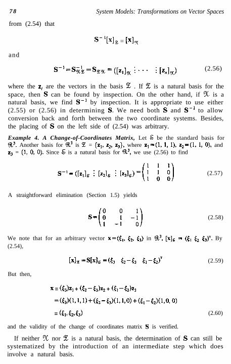
7 8
from (2.54) that
System Models: Transformations on Vector Spaces
s- ‘[xl2 = [XIX
and
s-1=$& =s,, = ([Zll% : * ’ l : P&J (2.56)
where the zi are the vectors in the basis % . If % is a natural basis for thespace, then S can be found by inspection. On the other hand, if % is anatural basis, we find S-l by inspection. It is appropriate to use either(2.55) or (2.56) in determining S. We need both S and S-i to allowconversion back and forth between the two coordinate systems. Besides,the placing of S on the left side of (2.54) was arbitrary.
Example 4. A Change-of-Coordinates Matrix, Let & be the standard basis for?R3. Another basis for ?Zk3 is % = {q, z,, z3}, where zl=(l, 1, I), z,=(l, 1, 0), andz3 = (1, 0, 0). Since & is a natural basis for a3, we use (2.56) to find
(2.57)
A straightforward elimination (Section 1.5) yields
s=(f -p 4) (2.58)
We note that for an arbitrary vector x=(tt, t2, t3) in $k3, [xl6 = (tl [, 53)T. By(2.54),
(2.59)
But then,
x = (53)z* + (52 - 531% + (5, - 52b3
=(53)(1,1,1)+(52-53)(1,1,0)+(51-52)(1,0,0)
= tt,, 52953) (2.60)
and the validity of the change of coordinates matrix S is verified.
If neither % nor FZ is a natural basis, the determination of S can still besystematized by the introduction of an intermediate step which doesinvolve a natural basis.

Sec. 2.5 Matrices of Linear Transformations 79
Exercise 3. Suppose we need the change-of-coordinates matrix S suchthat S[x]% = [xl%, where neither 5% nor % is a natural basis for ‘v.Suppose 97, is a natural basis. Show, by introducing an intermediatechange to the coordinates [xl%, that
S=([z,]s : ‘a * i [z.]J’([x& : ** - : [x,],) (2.61)
Example 5. Change of Coordinates via an Intermediate Natural Basis. Two bases
for 5Yp3 are 9 5 (4, f2, f3> and 8 f {gl, gz, g3}, where
f,(t)=l, f*(t)=l+t, f,(t)=l+P
g,(t)= 1+ t, gJt)= t, gJt)= t+ t2
To find S such that S[fj9 = [fig, we introduce the natural basis 5% i (h,, h2, h3},where hi(t) = t j- ‘. Then, by (2.61),
s= ([g& .: [g,], i [g&J1([fll~ 3 P21, : [f3ld
-(b 8 g)-‘(g d i))
=(-; 8-y& b ;!I=(-6 i-i)
Similarity and Equivalence Transformations
Now that we have a process for changing coordinate systems, we explorethe effect of such a change on the matrix of a transformation. Suppose T isa linear operator on V, and that 5% and % are two different bases for V.Then CT],, is defined by
Pl,,wx =Pln
The change from the % to the % coordinate system is described by
s[Jd% = [xl2
The change-of-coordinates matrix S also applies to the vector TX in ?r :
WY x = [TX1 %

80 System Models: Transformations on Vector Spaces
By substituting [xl, and [TX]% from these last two equations into thedefining equation for [TX],, , we find
[T],,S-‘[xl, =S-‘[TX],,
(S[Tl,,S-‘)[xl, = [TX],
But this is the defining equation for [T],,. It is apparent that
[TIE% =S[T],,S-’ (2.62)
where S converts from the % coordinate system to the % coordinatesystem. Equation (2.62) describes an invertible linear transformation on
mx, known as a similarity transformation. In Section 4.2, we find that asimilarity transformation preserves the basic spectral properties of thematrix. It is comforting to know that any two matrix representations of alinear system have the same properties-these properties are inherent inthe model, T, and should not be affected by the coordinate system weselect.
Example 6. A Similarity Transformation. In Example 2 we found the matrix ofthe differential operator on 9’ relative to the natural basis for 9”:
Another basis for 9’ is 9 = {gl, g2, g3}, where g*(t) = 1+ t, g2(t) = t, and g3(t) = t +t2. The change-of-coordinates matrix which relates the two bases 9Z and 9 isdefined by S[fJa =[f’j I ; we find it using (2.56):
The inverse matrix is

Sec. 2.6 Problems and Comments 81
Then, by (2.62),
Exercise 4. Let T: Y+%!l$ be a linear transformation. Assume ‘v and%’ are finite dimensional. Let the invertible matrix SXs convert from thebasis 5% to the basis 3 in V. Let the invertible matrix S,, convert fromthe basis 3 to the basis 8 in %. Show that
(2.63)
This transformation of the matrix [T],, is called an equivalence trans-formation. The similarity transformation (2.42) is a special case. The term“equivalence” is motivated by the fact that [T],, and [T],@ are equiva-lent models of the system. The system equation TX= y is equally wellrepresented by the matrix equations which result from the introduction ofany coordinate systems for V and W.
The discussion of matrices of transformations has been limited totransformations on finite-dimensional vector spaces. The primary reasonfor avoiding the infinite-dimensional counterparts is our inability to speakmeaningfully about bases for infinite-dimensional spaces before discussingconvergence of an infinite sequence of vectors (Section 5.3). However,matrices of infinite dimension are more difficult to work with (to invert,etc.) than are finite-dimensional matrices.
2.6 Problems and Comments
*2.1 Let 5, and S, be subsets of a vector space Ir. Let W, and %, besubspaces of V.(a) The intersection S r n S, of the sets S, and S, is the set of
vectors which belong to both S, and $5,; if S I n S, is emptyor if S,n S,= 8, we say S, and S, are disjoint.
(b) The union $5, u $5, of the sets $5, and S, is the set of vectorswhich belong either to 5, or to S, or to both.

8 2 System Models: Transformations on Vector Spaces
(c) The sum S i + S, of the sets S i and S, is the set of vectors ofthe form xi +x2, where xi is in S i and x2 is in S,.
(d) ‘%Y, n 9.l!‘, is a subspace.(e) 5!$, u %!YZ is usually not a subspace.(f> %, + “ru;, is the subspace spanned by %, u %,.(g) dim(‘?6,)+dim(‘%,)=dim(~,+~J+dim(~,n %J.
2.2 Prove that the real 3-tuple space s3 introduced in Equation (2.2) isa vector space.
2.3 Determine whether or not the following sets of vectors are linearlyindependent:(a) The column vectors (2 1 0 1)T, (1 2 -1 1)T, and (3 0 1 1)T
in %4x1(b) The functions f,(t)= 1+2t- t2, f,(t)=2+2t+ t2, a n d f3(t)
in 9’.(c) The functions gl(t)= 1+2t + t2- t3, g2(t)= 1 + t - t2+ t3, and
g3(t)= 1 +3t+3t2-3t3 in 5Y4.*2.4 Modulo-2 scalars: data transmitted by radio or telephone usually
consist in strings of binary numbers (ones and zeros). A characteror number to be transmitted is represented by a binary code wordof length n. It is a sequence of these code words which makes upthe transmitted string. We can think of the set of all possible codewords of length n as vectors in a vector space. We call the space abinary linear code (see [2.8]). The scalars used in vector spacemanipulations can be restricted to binary numbers if ordinaryaddition of scalars is replaced by modulo-2 addition:
o+o=o O+l=l
l+O=l l+l=O
The rules for multiplication of scalars need not be changed. Oneway to check for errors in data transmission is to let the nthelement of each code word equal the sum (mod-2) of the otherelements in the word. If a single error appears in the transmittedword, the nth element will fail to give the proper sum.(a) Let V be the set of 5 x 1 matrices with the mod-2 scalars as
elements. Show that ‘v is a vector space. (Assume that addi-tion and scalar multiplication of the matrices is based on themod-2 scalars.)
(b) Let %Y be the subset of ‘V consisting in vectors for which thefifth element equals the sum of the other four elements. Showthat % is a subspace of V.
(c) Find a basis % for %. Determine [xl,, where x = (1 1 0 11)T.

Sec. 2.6 Problems and Comments 8 3
(d) The subspace (?!lJ is a binary linear code. A code can also bedescribed by a “parity check” matrix P for which the code isthe nullspace. Find the parity check matrix for the code %.
2.5 The set of all real m x n matrices, together with the usual defini-tions of addition and scalar multiplication of matrices, forms avector space which we denote by ‘?Xmxn. Determine the dimensionof this linear space by exhibiting a basis for the space.
*2.6 Let Ir and % be vector spaces. With the definition of linearcombination of transformations given in (2.27),(a) The set of all transformations from V into Gtl(; forms a vector
space.(b) The set C( V, W) of all linear transformations from ?r into
‘?l! forms a subspace of the vector space in (a).(c) The set of all linear transformations which take a particular
subspace of V into 8, constitutes a subspace of I?( Ir, %).(d) If dim(Y)= n and dim(%)=,, then dim(E(‘V,%))=mn.
*2.7 Exploring linear combinations by row reduction. Let % 9 (y,, . . . , y,>be a set of m x 1 column vectors. The linear combination y= 2y, + * l l + c,y, can be expressed as y= Ax by defining
A = ( yi i y2 i . . . i y,) and x k (c, . . . c,)‘. Row reduction of the
matrix (A i y) for an unspecified vector y A (7,. . - qJT, or theequivalent row reduction of (A : I) for an m X m matrix I, deter-mines the form of the vectors in span( 3 ) and pinpoints any lineardependency in the set % . If 9 is linearly independent, the rowreduction also determines the coordinates with respect to % ofeach vector y in span( ‘3 ). Let
y=( g, yl=( a)¶ Y2=( ;J y3=( g9 y4=( a,
(a) Row reduce (A i I).(b) Determine the space spanned by % ; that is, determine the
relationships that must exist among the elements {qi} of y inorder that y be some linear combination of the vectors in % .Determine a basis for span( % ).
(c) Determine which linear combinations of the vectors in %equal the specific vector y given above.
(d) The form of span( % ) can also be determined by row reduc-tion of A’. The nonzero rows of the row-reduced matrixconstitute a basis for span( 9 ). Any zero rows which appearindicate the linear dependence of the set ‘% .

8 4 System Models: Transformations on Vector Spaces
2.8 For the following sets of vectors, determine if y is in span{y,}. If so,express y as a linear combination of the vectors {y,}.
(a) y=(i), YI=( $ Y249 Y3= (4)
(b) y=(i), YI=($ Y2=($ y3= (i>
(c) y=(;;)9 yl=(;). y2=(99 y3=('i)
2.9 Find a basis for the subspace of C?’ spanned by the functionsfl(t)= 1+ t +2t2, f2(t)=2t+ t2+ t3, and f3(t)=2+3t2- t3. Extendthe basis for the subspace to a basis for C?’ by adding appropriatevectors to the basis.
2.10 Find the coordinate matrix of the vector x= (1, 1, 1) in %k3:(a) Relative to the basis 5% = { (1, 0, 0), (1, -1, 0), (0, 1, -1)).(b) Relative to the basis 3 = {( 1, 1, -l), (1, -1, l), (-1, 1,
l>>*2.11 Find the coordinate matrix of the function f relative to the basis
9 = {gi, g,, g3}, where f(t) i t, gl(t) f l+ t, g2(t) 9 l+ t2, andg3( t) = 1 - t2.
2.12 Find the coordinate matrix of the function g relative to the basis
?F= {fl, f,, f,}, where f,(t) i 1- t, f2(t) i 1- t2, f,(t) 2 1 + t - t2,
and g(t) b & +[,t +c3t2.2.13 Find the coordinates of the vector x in ‘%2x2 relative to the basis
%L = (xl, x2, x3, x4}, where
2 14 Let ?P2x2 denote the space of polynomial functions of the form.f(s, t)= aI, + a,,s+ a,,t + a,,st. Find a basis for C!?2x2 which in-cludes the function f&s, t) = 2s - t - 1. Find the coordinate matrixof the general vector f in C?2x2 relative to that basis.
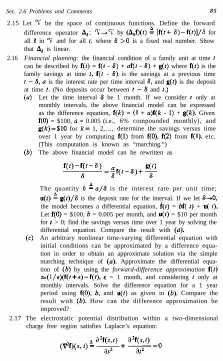
Sec. 2.6 Problems and Comments 85
2.15 Let 1/ be the space of continuous functions. Define the forward
difference operator A,,: Ir+V by (A,f)(t) A [f(t+ &)-f(t)]/6 forall f in ‘V and for all t, where 6 >0 is a fixed real number. Showthat As is linear.
2.16 Financial planning: the financial condition of a family unit at time tcan be described by f(t) = f(t - 6) + af(t - 6) + g(t) where f(t) is thefamily savings at time C, f(t - 6) is the savings at a previous timet - 8, a is the interest rate per time interval 6, and g(t) is the depositat time t. (No deposits occur between t - 8 and t.)(a) Let the time interval 6 be 1 month. If we consider t only at
monthly intervals, the above financial model can be expressedas the difference equation, f(k) = (1 + a)f(k - 1) + g(k). Givenf(0) = $100, a = 0.005 (i.e., 6% compounded monthly), andg(k)=$lO for k= 1, 2,…, determine the savings versus timeover 1 year by computing f(1) from f(O), f(2) from f(l), etc.(This computation is known as “marching.“)
(b) The above financial model can be rewritten as
The quantity b i a/8 is the interest rate per unit time;
u(t) 4 g(t)/6 is the deposit rate for the interval. If we let 6+0,the model becomes a differential equation, f(t) = bf( t) + u( t).Let f(0) = $100, b = 0.005 per month, and u(t) = $10 per monthfor t > 0; find the savings versus time over 1 year by solving thedifferential equation. Compare the result with (a).
(c) An arbitrary nonlinear time-varying differential equation withinitial conditions can be approximated by a difference equa-tion in order to obtain an approximate solution via the simplemarching technique of (a). Approximate the differential equa-tion of (b) by using the forward-difference approximation f(t)w(l/C)(f(t+E)-f(t), e = 1 month, and considering t only atmonthly intervals. Solve the difference equation for a 1 yearperiod using f(O), b, and u(t) as given in (b). Compare theresult with (b). How can the difference approximation beimproved?
2.17 The electrostatic potential distribution within a two-dimensionalcharge free region satisfies Laplace’s equation:
A a2f(s9t) + a2f(&t) =.(.V2f)(s, t) = ~ -
as2 at2

86 System Models: Transformations on Vector Spaces
For the potential distribution between two parallel plates of spac-ing d, the model reduces to f”(s)=0 with f(0) and f(d) given.(4
(b)
cc>
Assume the differential operator D2 acts on e2(0,d), a spaceof twice-differentiable functions. Find the nullspace of D2, asubspace of e2(0,d). The nullspace is the solution space forthe above differential equation. Express the solution space interms of the known boundary values f(0) and f(d). What is thedimension of the nullspace of D2?Define the central-difference operator A on e2(0,d) by
(Af)(s) i f(s+ $) -f(s- ;)
The derivative of f can be expressed as the limit of thecentral-difference approximation, f’(s)w(Af)(s)/& Verify thatD2, as it acts on L?‘(O,d), can be approximated arbitrarilyclosely by the second-central-difference approximation, D2WA2/iS2.Suppose the plate spacing is d = 5. Let 6 = 1, and evaluate thefinite-difference approximation A2f = 8 at s = 1, 2, 3, and 4 toobtain four algebraic equations in the variables f(O),f(l) , . . . ,f(5). Formulate these algebraic equations as a 4 X 6matrix equation Ax= 8. Compare this matrix equation withthe differential equation D2f = 8; that is, compare the spaceson which the operators act; also compare the dimensions oftheir solution spaces. Solve the matrix equation in terms of theboundary values f(0) and f(5). Compare the discrete solutionwith the continuous solution found in (a).This problem can also be carried out for the two-dimensionalcase, where f(s, t) is given on a closed boundary. The finite-difference approach in (b) and (c) is widely used in thesolution of practical problems of this type. The equations,sometimes numbering as many as 100,000, are solved byiterative computer techniques. See Forsythe and Wasow [2.4].
2.18 According to the trapezoidal rule for approximate integration, if wesubdivide the interval [a, b] into n segments of length 6, and denoteg(a+j8) by 6, j=O, l,..., n, then for a continuous g,

Sec. 2.6 Problems and Comments 87
We can view the trapezoidal rule as an approximation of a functionspace integral operation by a matrix multiplication Ax, where A is
lxn andxi(go.+.g,JT.(a) Find the matrix A which expresses the trapezoidal rule for
6 = 1 and n = 5. Apply the trapezoidal rule to accurately repre-
sent the integral of the discontinuous function g(s) e 1 for
0 < s < 2, g(s) 4 0 for 2 < s < 5. Hint: at the discontinuity usethe midpoint value, (g; + gT)/2.
(b) We can also approximate a general integral operator by a
matrix multiplication. Suppose (Tf)(t) s jik(t,s)f(s) ds for tin [a, b]. We can treat the function k(t, s)f(s) as we did g(s) in(a). Subdivide both the s and t intervals into n segments oflength 6, and use the same subscript notation for functionvalues as above. Then if k(t,s)f(s) is continuous,
for j=O, I,..., n. We can approximate the integral operationby a matrix multiplication, y = Ax, where x = (foe 0 . f,)’ andY = ((TOO * . . (Tf),,)‘. Find A for 6= 1, n=5, a=O, b=5, and
Hint: use midpoint values as in (a). Note that the operator isordinary indefinite integration.
(c) Apply the matrix multiplication found in (b) to obtain theapproximate integral of f(s) = 3s2. Compare the approximationto the actual integral at the points t = 0, 1,…,5.
*2 19. Exploring the nullspace and range by row reduction: Let
Multiplication by A is a linear transformation from %4x1 into(?liL3x ‘. Multiplication by AT is a linear transformation from a3 x ’into YlL4” ‘. In Section 5.4 we find that if y is in range(A) and x isin nullspace(A9, then x l y = 0 where x l y is the dot product ofanalytic geometry. Furthermore, if z is in range(AT) and w is in

88 System Models: Transformations on Vector Spaces
nullspace( then z l w = 0. By means of these dot product equa-tions, we can use bases for nullspace(A3 and range(A3 to findbases for range(A) and nullspace( and vice versa. We can alsoshow that rank(A) =rank(A’). In this problem we obtain null-space(A) and range(A) directly from A’.(a) Row reduce (A i I). Use the results of the row reduction to
determine bases for nullspace and range(A).(b) Row reduce (A’ : I). Show that the nonzero rows in the
left-hand block of the row-reduced matrix constitute a basisfor range(A). Show that the rows of the right-hand blockwhich correspond to zero rows of the left-hand block of therow-reduced matrix constitute a basis for nullspace(
2.20 Define T: $P3+ C? (0, 1) by (Tf)(t) B jAk( t,s)f(s) ds for all f in C?‘,where
k(t,s)= t(1 -s) f o r t < s
=(1-t)s f o r t>s
Find a basis for range(T). Describe nullspace(
2.21 Let % be the space of polynomial functions f of the form
f(s, t) f c, + c2s + c,t + c,st for all s and t. Define T: w +G2l(i by
(Tf)(s, t) 9 (a/%)f(s, t) for all f in % .(a) Find a basis for the range of T.(b) Determine the rank and nullity of T.
2.22 Define T: 9’lL2x2+911,2x2 by
T( :; f:) 9 ( y2 c4cIc3)
for all choices of the scalars cl, c2, c3, and c4. Find nullspace andrange(T) by exhibiting a basis for each.
2.23 Expected value: the throws of a single die constitute an experiment.Let II‘ be the space of random variables defined on this experi-ment. We can think of the probability mass function a(u) as therelative frequency with which the outcome u occurs: o(a) = d foru=l, 2 ,..., 6.(a) A random variable x in V associates a value x(a) with each
possible outcome of the experiment. The value which xassociates with an actual trial of the experiment is called asample value of x. The probability mass function o,(x) speci-fies the relative frequency with which the sample value xoccurs during repeated trials. Find w,(y) for the random

Sec. 2.6 Problems and Comments 89
2.24
variable y defined by y(a) 4 2 for 0 = 1 or 2 and by y(a) 4 0for u=3, 4, 5, or 6.
(b) The expected value of x is the average, over many trials, of thesample values of x. Thus
Find E(y) for the random variable y given in (a).(c) Show that the functional E: v+% is linear. Pick a basis %
for V. Let & g {(1)} be a basis for 3. Find [y]% and [ElxXG,where y is the random variable in (a).
(d) If f: ?r+ V then f(x) is a random variable. Express E (f(x)) interms of o(u). Find E(y2) for the random variable y given in(a). If g: Ir x V+ Ir, can E be applied to g(x, y)?
Hadamard matrices: let f(s) represent the light intensity versusposition in one line of a television picture. Let the n x 1 columnvector x be a discrete approximation to f. Then x can be viewed asa one-dimensional photograph. Suppose the data x must be trans-mitted for remote viewing. One way to reduce the effect of trans-mission errors and to reduce the amount of data transmitted is totransmit, instead, a transformed version of x. A computationallysimple transformation is the Hadamard transform—multiplicationby a Hadamard matrix. A symmetric Hadamard matrix H consistsin plus and minus ones, and satisfies H-l = H (see [2.9]). Denotethe transformed vector by X = Hx. Let n = 8 and
The Hadamard transform spreads throughout the elements of X theinformation which is concentrated in a single element of x; itconcentrates information which is spread out.(a) D e t e r m i n e t h e e f f e c t o f H o n t h e p h o t o g r a p h s x
=(11111111)T and x = &i, where q is the ith standard basisvector for %8x1.

90 System Models: Transformations on Vector Spaces
2.25
(b) Find the transform of the photograph x = (2 2 2 3 2 2 2 2)T. As-sume that an error during transmission of X reduces the thirdelement of X to zero. Determine the effect of the error on thereconstructed photograph.
(c) The inverse transform, x= HX, can be interpreted as anexpansion of x in terms of the columns of H. The columns ofH are analogous to sinusoidal functions; the number of zerocrossings corresponds to frequency. Let x be the photographin (b). Determine the effect on the reconstructed photographof not transmitting the highest frequency component of X (i.e.,the effect of making the second element of X zero). Determinethe effect on the reconstructed photograph of eliminating thezero frequency component (i.e., the effect of making the firstcomponent of X zero).
The space C?‘(O, cc) consists in the continuously differentiable func-tions on [0, co]. Define the Cartesian product space ?r by
Yi el(o,w)>: ..’ x E?‘(O, cc). Denote the vector-valued func-n-1
tions in Ir by x. We can treat the values of x as vectors in ?Rn x I;that is, x(t)=(f,(t). * . f,(t))‘, where fj is in C?‘(O, 00). Let A be a realn x n matrix. Define the linear transformation T: V+ % by
This transformation is central to the state-space analysis ofdynamic systems.(a) Determine an appropriate range of definition %$ for T.(b) Find a basis for nullspace if n = 2 and
2.26 Assume e < 6~ 1. Then the following matrix is nearly singular:
Use inverse iteration to find a basis for the near nullspace of A.
2.27 Define T: CR,*+ CR,* by ‘JXl, t2) i (Cl + 2t2,t1 - 25,) for all (cl,<*) inCR,*. Let % = {(1, l), (1, -l)}. Find [T],,.
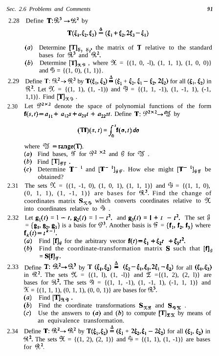
Sec. 2.6 Problems and Comments 91
2.28
2.29
2.30
2.31
2.32
2.33
2.34
Define T: by
(a) Determine [TIF, G2, the matrix of T relative to the standardbases for CR3 and Ck2.
(b) Determine [T],, , where % = {(1, 0, -l), (1, 1, 1), (1, 0, 0)}and % = {(1, 0), (1, 1)}.
Define T: C?L2-+ CR3 by T(5,, t2) f (Cl + t2, & - t2, 2t2) for all (&, t2) in%2. Let % = {(1, 1), (1, -1)) and ‘% = {(1, 1, -1), (1, -1, 1), (-1,1,1)}. Find [T],, .
Let C?2x2 denote the space of polynomial functions of the formf(s,t)=a,,+ a,,s+a,,t + a,,st. Define T: C?2x2+W by
(Tf)(s, t) = jsf(u, t)du0
where ‘%’ =range(T).(a) Find bases, g for q2 x2 and 9 for qti .(b) Find [T],, .(c) Determine T- ’ and [T- I]@%. How else might [T- ‘lgF be
obtained?The sets % = {(1, -1, 0), (1, 0, 1), (1, 1, 1)} and 3 = {(1, 1, 0),(0, 1, 1), (1, -1, 1)} are bases for $k3. Find the change ofcoordinates matrix S,, which converts coordinates relative to 5%into coordinates relative to %I .
Let gl(t) = 1 - t, g2(t) = 1 - t2, and g3(t) = 1 + t - t2. The set 4= {g,, g,, g3} is a basis for 03. Another basis is % = {f,, f2, f3} wheref/Jt)= P-'.(a) Find [f], for the arbitrary vector f(t)=tl +t2t +c3t2.(b) Find the coordinate-transformation matrix S such that [fle
= S[f],.
Define T: Cfi,2+a3 by T (t1,t2) e (5‘2-5,,51,251-52) for all &,S,>in Ck2. The sets % = {(1, l), (1, -l)} and % ={(1, 2), (2, l)} arebases for Ck2. The sets ‘% = {(1, 1, -1), (1, -1, 1), (-1, 1, 1)} andx = {(1, 1, 1), (0, 1, 1), (0, 0, 1)} are bases for C!R3.(a) Find [T],, .(b) Find the coordinate transformations S,, and S,, .(c) Use the answers to (a) and (b) to compute [T],, by means of
an equivalence transformation.
Define T: a2+ a2 by T(5,,t2) 9 (tr + 2t2,5, - 2t2) for all (tl, t2) in$k2. The sets 5% = {(1, 2), (2, 1)} and % = {(1, 1), (1, -1)} are basesfor CR2.

92 System Models: Transformations on Vector Spaces
(a) Find [T]%,,.(b) Find the coordinate transformation S,, .(c) Use the answers to (a) and (b) to compute [T], q by means of
a similarity transformation.
2.35 Multiplication by an invertible matrix can be interpreted either as alinear transformation or as a change of coordinates. Let CX ={x1,x2} be a basis for a two-dimensional space ‘V and x a vector in
V. Then [x,1% = (A) and [x2]% = (7). Let
(a) Alias interpretation: assume A[x]~ =[x]~ , where % = {yl,y2}is a second basis for ‘Ir. Find [ylln and [y2]%. Sketch [xJ~,[X21Xx [Xl%? [Y,lw and [y21n as arrows in a plane. What is therelationship between [xl% and the basis {[yljX, [y2]%}; thatis, what is meant by the notation [xl% ?
(b) Alibi interpretation: assume A[x], =[Tx],. Sketch [x,]~,
[x215% 9 [Xl% 9 and [TX], as arrows in a plane. What is therelationship between [TX], and the basis {[xJX, [x21X}; thatis, what is meant by the notation [TX],?
2.7 References
[2.1]
[2.2]
[2.3]
[2.4]
*[2.5]
*[2.6]
[2.7]
[2.8]
[2.9]
[2.10][2.11]
Churchill, R. V., Fourier Series and Boundary Value Problems, McGraw-Hill, NewYork, 1941.Cramer, Harald and M. R. Leadbetter, Stationary and Related Stochastic Processes,Wiley, New York, 1967.Forsythe, George E., “Singularity and Near Singularity in Numerical Analysis,” Am.Math. Mon., 65 (1958), 229-40.Forsythe, George E. and Wolfgang R. Wasow, Finite Difference Methods for PartialDifferential Equations, Wiley, New York, 1960.Halmos, P. R., Finite-Dimensional Vector Spaces, Van Nostrand, Princeton, N. J.,1958.Hoffman, Kenneth and Ray Kunze, Linear Algebra, Prentice-Hall, Englewood Cliffs,N. J., 1961.Papoulis, Athanasios, Probability, Random Variables, and Stochastic Processes,McGraw-Hill, New York, 1965.Peterson, W. Wesley, Error-Correcting Codes, M.I.T. Press and Wiley, New York,1961 .Pratt, William K., Julius Kane, and Harry C. Andrews, “Hadamard TransformImage Coding,” Proc. IEEE, 57, 1 (January 1969), 58-68.Royden, H. L., Real Analysis, 2nd ed., Macmillan, New York, 1968.Wylie, C. R., Jr., Advanced Engineering Mathematics, 3rd ed., McGraw-Hill, NewYork, 1966.