system-level modeling and optimization of mimo hsdpa...
TRANSCRIPT
DISSERTATION
System-Level Modeling and Optimizationof MIMO HSDPA Networks
Conducted for the purpose of receiving the academic title“Doktor der technischen Wissenschaften”
Dipl.-Ing. Martin WrulichMatrikelnummer: 9961105
Neubaugasse 47/19, 1070 Wien, Austria
November 20, 2009
Submitted at Vienna University of TechnologyFaculty of Electrical Engineering and Information Technology
Vienna, September 2009


For those I love.

Supervisor
Univ.Prof. Dr.-Ing. Dipl.-Ing. Markus RuppInstitut fur Nachrichtentechnik und Hochfrequenztechnik
Technische Universitat Wien, Osterreich
Examiner
Prof. Dipl. El.-Ing. ETHZ, Dipl. Math. ETHZ, Dr. Sc. Techn. (ETHZ) BernardHenri Fleury
Department of Electronic SystemsAalborg Universitet, Denmark

Abstract
Interaction between the Medium Access Control (MAC)-layer and the physical-layer routinesis one of the basic concepts of modern wireless networks. Physical-layer dependent resourceallocation and scheduling guarantee efficient network utilization. Accordingly, classical link-levelanalyses, focusing only on the physical-layer are not sufficient anymore for optimum transceiverstructure and algorithm development.
This thesis presents the development and application of a system-level description suitablefor the downlink of Multiple-Input Multiple-Output (MIMO) enhanced High-Speed DownlinkPacket Access (HSDPA), with particular focus on the Double Transmit Antenna Array (D-TxAA)transmission mode. The system-level model allows for investigating and evaluating transmissionsystems and algorithms in the context of cellular networks. Two separate models are proposedto obtain a complete system-level description: (i) a link-quality model, analytically describingthe MIMO HSDPA link quality in a so-called equivalent fading parameter structure, and (ii) alink-performance model, capable of predicting the BLock Error Ratio (BLER) performance ofthe transmission.
Based on this novel system-level model, a flexible system-level simulator is developed. The sim-ulator, implemented in Matlab, is subsequently applied to a set of different optimizations. First,some general investigations of the system behavior of D-TxAA MIMO HSDPA in the cellular net-work context are conducted. This leads to recommendations and guidelines for network planning.Afterwards a Radio Link Control (RLC) based D-TxAA stream number decision algorithm withenhanced robustness against outdated User Equipment (UE) Channel Quality Indicator (CQI)feedback is developed. Similarly, a novel content-aware Medium Access Control for High-SpeedDownlink Packet Access (MAC-hs) scheduler increasing the Quality of Experience (QoE) forvideo-streaming is proposed and its performance is assessed. Besides the research focusing onthe High-Speed Downlink Shared CHannel (HS-DSCH) also the signaling channels—being veryimportant for the operation of wireless networks—are investigated. In particular, an optimiza-tion of the Common Pilot CHannel (CPICH) power allocation for various network configurationsis conducted. The findings are especially important for MIMO HSDPA trials, but can also bevaluable for the optimization of already existing MIMO HSDPA cell clusters.
Finally, a multi-user interference-aware Minimum Mean Squared Error (MMSE) equalizer isdeveloped. This novel receiver takes the structure of the Transmit Antenna Array (TxAA)interference in the cell into account. The underlying system-model represents an extension tothe classical single-user analysis. The theoretical limits and the throughput are evaluated bymeans of physical-layer and system-level investigations under realistic channel conditions. Theresults show significant performance gains of the interference-aware equalizer for channels withlarge delay spread.
vii


Kurzfassung
Die Einbindung der Medium Access Control (MAC)-schicht in Vorgange der Bitubertragungs-schicht ist eines der grundlegenden Konzepte moderner Funknetzwerke. Die Allokation unddas Scheduling passend zur Bitubertragungsschicht garantiert eine effiziente Ausnutzung derNetzwerk-Ressourcen. Das bedeutet jedoch auch, dass die klassische Betrachtung der Uber-tragungsstrecke—mit Fokus auf die Bitubertragungsschicht—nicht mehr ausreicht um optimaleSende- und Empfangsstrukturen sowie Algorithmen zu entwickeln.
Diese Dissertation prasentiert die Entwicklung und einige Anwendungen eines system-levelModells, das geeignet ist, den Downlink von Mehrfachantennen (MIMO) High-Speed DownlinkPacket Access (HSDPA) darzustellen. Besonderer Fokus wird dabei auf den Double TransmitAntenna Array (D-TxAA) Ubertragungsmodus gelegt. Das vorgeschlagene Modell erlaubt dieUntersuchung und das Testen von Ubertragungssystemen und Algorithmen im Kontext von zel-lularen Netzwerken. Um eine vollstandige Systembeschreibung zu erhalten, werden zwei getren-nte Modelle entwickelt: (i) ein link-quality Modell, welches die MIMO HSDPA Verbindungs-qualitat analytisch in einer sogenannten aquivalenten Schwund-Parameter-Struktur darstellt,und (ii) ein link-performance Modell, welches eine Vorhersage der Blockfehlerrate (BLER) derUbertragung ermoglicht.
Basierend auf diesem neuen System-Modell wird außerdem ein neuartiger, flexibler system-levelSimulator entwickelt. Der in Matlab implementierte Simulator wird anschließend fur eine Reihevon Optimierungen verwendet. Zuerst wird eine allgemeine Untersuchung der System-Leistungvon D-TxAA MIMO HSDPA im Kontext zellularer Netzwerke durchgefuhrt. Die gewonnenErkenntnisse fuhren zu einigen Empfehlungen und Richtlinien fur die Funknetzplanung. Danachwird ein Radio Link Control (RLC) basierender Algorithmus entwickelt und getestet, welcherfur D-TxAA die geeignete Anzahl der parallelen Sendestrome ermittelt. Der Algorithmus ze-ichnet sich insbesondere durch eine erhohte Robustheit gegen Fehler bei den Kanalqualitats-Ruckmeldungen der mobilen Endgerate aus. Anschließend wird ein neuer Scheduler vorgestellt,welcher Informationen uber den Inhalt der zu ubertragenen Pakete verwendet um die Qualitatvon gestreamten Videos zu erhohen. Neben der Forschung mit Fokus auf den HSDPA Datenkanal(HS-DSCH) werden auch die Signalisierungskanale—welche sehr wichtig fur das Betreiben vonFunknetzwerken sind—untersucht. Insbesondere wird die optimale Leistungsverteilung des Pilot-Kanals (CPICH) fur unterschiedliche Netzwerk-Konfigurationen bestimmt. Die gewonnen Erken-ntnisse sind sehr wichtig fur MIMO HSDPA Testversuche, aber auch fur die Optimierung voneventuell schon bestehenden MIMO HSDPA Zellgruppen.
Abschließend wird ein Minimum Mean Squared Error (MMSE) Entzerrer entwickelt, der dieInterferenz-Struktur von Transmit Antenna Array (TxAA) Ubertragungen berucksichtigt. Daszugrundeliegende System-Modell ist eine Erweiterung der klassischen Einfachnutzer Sichtweise.Durch Simulationen der Funkubertragungsstrecke und system-level Simulationen werden sowohldie theoretischen Limits als auch die Datendurchsatz-Leistungsfahigkeit unter realistischen Be-dingungen untersucht. Die Ergebnisse zeigen beachtliche Leistungsgewinne des vorgeschlagenenEntzerrers bei Funkkanalen mit großen Laufzeiten.
ix

AcknowledgementsThe only people with whom youshould try to get even are those whohave helped you.
(John E. Southard)
A dissertation is a big challenge, being a both painful and enjoyable experience. It is just likeclimbing a mountain, step by step, accompanied with hardships and frustration, but also withencouragement and kind help of many people. The following pages are the result of this pathand contain a lot of the knowledge I was able to acquire during my time as a doctoral candidate.Going through the process of uniting the individual results, findings, and concepts for the thesisis—in my eyes—necessary to develop the kind of academic appreciation that lies in the heart ofevery scientist. Now, at the top of the mountain, I realize that without the support of manygreat people I would not have come that far, and thus I owe them my sincere gratitude.
First of all, I have to thank my supervisor, Prof. Markus Rupp. The possibility to engage in theresearch of wireless networks, and the liberty to freely pursue all topics and ideas that appearedinteresting to me, was wonderful. Furthermore, his academic advises were an indispensable helpthroughout my whole dissertation. Similar holds for my second examiner, Prof. Bernard Fleury. Ihad the pleasure to enjoy his thoughtful guidance as a project leader, and I owe him my gratitudefor accepting my invitation to be my co-examiner.
My many, many thanks additionally have to go to mobilkom austria AG as a whole for sup-porting my thesis financially, but also in particular to Dr. W. Wiedermann, W. Weiler, andM. Koglbauer for many fruitful discussions and the provided data. Appreciation likewise belongsto the ftw, allowing me to participate in two interesting projects where I had the chance tomeet Dr. S. Eder (Siemens AG) and Dr. I. Viering (Nomor GmbH). The joint work with themcontributed a lot to my scientific understanding of system-level research. Moreover, I want toemphasize my gratitude for Prof. A. Paulraj, who made it possible for me to join his group atStanford University for a short period. The time as a visiting researcher broadened my knowledgein the field and helped me to bring the thesis to its current form.
Of course, a great amount of thankfulness also belongs to my colleagues at the institute, espe-cially to Dr. C. Mehlfuhrer who shared his expertise and friendship with me. I am furthermoreindebted to G. Lilley, L. Superiori, A. Mateu, and J. Colom Ikuno for the joint work and theirsupport, as well as to Dr. L. W. Mayer for his patient help on the textual presentation of thisthesis.
Last but not least, I want to thank my parents Ingeborg and Ferdinand, as well as my sisterElisabeth. I owe everything to them, their warm disposition and their unshakable trust in mecan not be compensated. Finally, for all the times she stood by me, and all the joy she broughtto my life, I want to thank my love, Gloria Wind.
xi

Contents
List of Figures xvii
List of Tables xix
1. Introduction 11.1. Motivation for this Dissertation . . . . . . . . . . . . . . . . . . . . . . . . . . . . 11.2. Scope of Work and Contributions . . . . . . . . . . . . . . . . . . . . . . . . . . . 4
2. HSDPA and its MIMO Enhancements 92.1. HSDPA Principles . . . . . . . . . . . . . . . . . . . . . . . . . . . . . . . . . . . 10
2.1.1. Network Architecture . . . . . . . . . . . . . . . . . . . . . . . . . . . . . 102.1.2. Physical Layer . . . . . . . . . . . . . . . . . . . . . . . . . . . . . . . . . 122.1.3. MAC Layer . . . . . . . . . . . . . . . . . . . . . . . . . . . . . . . . . . . 162.1.4. Radio Resource Management . . . . . . . . . . . . . . . . . . . . . . . . . 16
2.2. MIMO Enhancements of HSDPA . . . . . . . . . . . . . . . . . . . . . . . . . . . 182.2.1. Physical Layer Changes . . . . . . . . . . . . . . . . . . . . . . . . . . . . 202.2.2. MAC Layer Changes . . . . . . . . . . . . . . . . . . . . . . . . . . . . . . 222.2.3. Simplifications of the Core Network . . . . . . . . . . . . . . . . . . . . . 22
3. System-Level Modeling of MIMO-Enhanced HSDPA 233.1. Concept of System-Level Modeling . . . . . . . . . . . . . . . . . . . . . . . . . . 243.2. Applicability of other Published Work . . . . . . . . . . . . . . . . . . . . . . . . 263.3. Computationally Efficient Link-Quality Model . . . . . . . . . . . . . . . . . . . . 27
3.3.1. Equalizer . . . . . . . . . . . . . . . . . . . . . . . . . . . . . . . . . . . . 283.3.2. WCDMA MIMO in the Network Context . . . . . . . . . . . . . . . . . . 303.3.3. Description of the Equivalent Fading Parameters . . . . . . . . . . . . . . 323.3.4. Generation of the Equivalent Fading Parameters . . . . . . . . . . . . . . 373.3.5. Influence of Non-Data Channels . . . . . . . . . . . . . . . . . . . . . . . 403.3.6. Resulting SINR Description . . . . . . . . . . . . . . . . . . . . . . . . . . 423.3.7. Validation . . . . . . . . . . . . . . . . . . . . . . . . . . . . . . . . . . . . 433.3.8. Complexity . . . . . . . . . . . . . . . . . . . . . . . . . . . . . . . . . . . 46
3.4. Link-Performance Model . . . . . . . . . . . . . . . . . . . . . . . . . . . . . . . . 483.4.1. Link-Performance Model Concept . . . . . . . . . . . . . . . . . . . . . . 503.4.2. Training and Validation of the Model . . . . . . . . . . . . . . . . . . . . 53
3.5. Summary . . . . . . . . . . . . . . . . . . . . . . . . . . . . . . . . . . . . . . . . 59
4. System-Level-Simulation-Based Optimization of MIMO-Enhanced HSDPA 614.1. MIMO HSDPA System-Level Simulator . . . . . . . . . . . . . . . . . . . . . . . 62
4.1.1. Detailed Simulator Structure . . . . . . . . . . . . . . . . . . . . . . . . . 634.1.2. Network Setup . . . . . . . . . . . . . . . . . . . . . . . . . . . . . . . . . 65
xiii
4.2. Network Performance Prediction . . . . . . . . . . . . . . . . . . . . . . . . . . . 694.2.1. Simulation Setup . . . . . . . . . . . . . . . . . . . . . . . . . . . . . . . . 694.2.2. Single Network Scenario Investigation . . . . . . . . . . . . . . . . . . . . 704.2.3. Average Network Performance . . . . . . . . . . . . . . . . . . . . . . . . . 72
4.3. RLC-Based Stream Number Decision . . . . . . . . . . . . . . . . . . . . . . . . . 754.3.1. UE Decision . . . . . . . . . . . . . . . . . . . . . . . . . . . . . . . . . . . 754.3.2. RLC Decision . . . . . . . . . . . . . . . . . . . . . . . . . . . . . . . . . . 764.3.3. System-Level Simulation Results . . . . . . . . . . . . . . . . . . . . . . . 76
4.4. Content-Aware Scheduling . . . . . . . . . . . . . . . . . . . . . . . . . . . . . . . 784.4.1. Introduction . . . . . . . . . . . . . . . . . . . . . . . . . . . . . . . . . . 784.4.2. Video Packet Prioritization in HSDPA . . . . . . . . . . . . . . . . . . . . 784.4.3. Content-Aware Scheduler . . . . . . . . . . . . . . . . . . . . . . . . . . . 794.4.4. Simulation Results . . . . . . . . . . . . . . . . . . . . . . . . . . . . . . . 80
4.5. CPICH Power Optimization . . . . . . . . . . . . . . . . . . . . . . . . . . . . . . 814.5.1. System-Level Modeling of the CPICH Influence . . . . . . . . . . . . . . . 824.5.2. CPICH Optimization in the Cellular Context . . . . . . . . . . . . . . . . 83
4.6. Summary . . . . . . . . . . . . . . . . . . . . . . . . . . . . . . . . . . . . . . . . 85
5. Multi-User MMSE Equalization for MIMO-Enhanced HSDPA 875.1. System Model . . . . . . . . . . . . . . . . . . . . . . . . . . . . . . . . . . . . . . 885.2. Intra-Cell Interference-Aware MMSE Equalization . . . . . . . . . . . . . . . . . 91
5.2.1. Interference Suppression Capability . . . . . . . . . . . . . . . . . . . . . . 935.2.2. Complexity . . . . . . . . . . . . . . . . . . . . . . . . . . . . . . . . . . . 96
5.3. The Cell Pre-Coding State . . . . . . . . . . . . . . . . . . . . . . . . . . . . . . . 965.3.1. Training-Sequence-based Pre-Coding State Estimation . . . . . . . . . . . 985.3.2. Blind Pre-Coding State Estimation . . . . . . . . . . . . . . . . . . . . . . 995.3.3. Estimator Performance . . . . . . . . . . . . . . . . . . . . . . . . . . . . 101
5.4. Performance Evaluation . . . . . . . . . . . . . . . . . . . . . . . . . . . . . . . . 1015.4.1. Physical-Layer Simulation Results . . . . . . . . . . . . . . . . . . . . . . 1025.4.2. System-Level Simulation Results . . . . . . . . . . . . . . . . . . . . . . . 103
5.5. Summary . . . . . . . . . . . . . . . . . . . . . . . . . . . . . . . . . . . . . . . . 105
6. Conclusions 107
A. Additional Material 111A.1. Standardization, Current Deployment of HSDPA . . . . . . . . . . . . . . . . . . 111A.2. Pre-Coding Codebook; Pre-Coding Evaluation . . . . . . . . . . . . . . . . . . . 113A.3. Additional Equivalent Fading Parameter Statics . . . . . . . . . . . . . . . . . . . 116A.4. Proof of Theorem 3.1 . . . . . . . . . . . . . . . . . . . . . . . . . . . . . . . . . . 117A.5. Further Link-Quality Model Validation Results . . . . . . . . . . . . . . . . . . . 119A.6. Discussion of Assumption 3.9 . . . . . . . . . . . . . . . . . . . . . . . . . . . . . 119A.7. Auxiliary System-Level Models . . . . . . . . . . . . . . . . . . . . . . . . . . . . 123
A.7.1. SINR-to-CQI Mapping . . . . . . . . . . . . . . . . . . . . . . . . . . . . . 124A.7.2. HARQ Modeling . . . . . . . . . . . . . . . . . . . . . . . . . . . . . . . . 125
A.8. Semi-Analytical System-Level Performance Bound . . . . . . . . . . . . . . . . . 126A.9. Video Coding and Video Quality Indicators . . . . . . . . . . . . . . . . . . . . . 127
A.9.1. Quality of Service Management . . . . . . . . . . . . . . . . . . . . . . . . 129
A.10.Additional CPICH Power Optimization Results . . . . . . . . . . . . . . . . . . . 129A.11.WCDMA Chip Energy and PSD Parameters . . . . . . . . . . . . . . . . . . . . 130A.12.Calculating the Effective Code-Rate . . . . . . . . . . . . . . . . . . . . . . . . . 131A.13.Validation of the System-Level Simulator with Odyssey Data . . . . . . . . . . . 131A.14.SINR Optimality of Interfernce-Aware MMSE Equalizer . . . . . . . . . . . . . . 133A.15.List of Most Important System-Level Simulator Settings . . . . . . . . . . . . . . 134
B. Further System-Level Modeling, Simulations, Optimizations, and Validation 137B.1. Mixed Traffic Optimization for SISO HSDPA . . . . . . . . . . . . . . . . . . . . 137
B.1.1. System Model . . . . . . . . . . . . . . . . . . . . . . . . . . . . . . . . . . 138B.1.2. Simulation Details . . . . . . . . . . . . . . . . . . . . . . . . . . . . . . . 142B.1.3. Results . . . . . . . . . . . . . . . . . . . . . . . . . . . . . . . . . . . . . 143
B.2. Link-Quality Model for STTD . . . . . . . . . . . . . . . . . . . . . . . . . . . . . 145B.2.1. System Model for STTD . . . . . . . . . . . . . . . . . . . . . . . . . . . . 146B.2.2. Computationally Efficient Link-Quality Model . . . . . . . . . . . . . . . 147B.2.3. Generation of the Equivalent Fading Parameters . . . . . . . . . . . . . . 150
List of Abbreviations 153
List of Symbols 157
Bibliography 161

List of Figures
1.1. Influence of the scheduler on the fading statistics . . . . . . . . . . . . . . . . . . 3
2.1. Network architecture for HSDPA . . . . . . . . . . . . . . . . . . . . . . . . . . . 102.2. Protocol design in UMTS . . . . . . . . . . . . . . . . . . . . . . . . . . . . . . . 112.3. Communication channel design of HSDPA . . . . . . . . . . . . . . . . . . . . . . 122.4. Multi-user transmission on the HS-DSCH . . . . . . . . . . . . . . . . . . . . . . 152.5. HSDPA timing relations . . . . . . . . . . . . . . . . . . . . . . . . . . . . . . . . 152.6. HSDPA power allocation principles . . . . . . . . . . . . . . . . . . . . . . . . . . 172.7. MIMO spatial multiplexing and diversity gain . . . . . . . . . . . . . . . . . . . . 192.8. Overview of the D-TxAA transmitter scheme . . . . . . . . . . . . . . . . . . . . 21
3.1. Wireless communication transmission chain . . . . . . . . . . . . . . . . . . . . . 253.2. System-level relations . . . . . . . . . . . . . . . . . . . . . . . . . . . . . . . . . 263.3. System model for a WCDMA system . . . . . . . . . . . . . . . . . . . . . . . . . 283.4. The ecdfs of equivalent fading parameters in the 2× 1 SS case . . . . . . . . . . . 383.5. The ecdfs of equivalent fading parameters in the 2× 2 DS case . . . . . . . . . . 393.6. Comparison of the distributions of the equivalent fading parameters . . . . . . . 413.7. Link-quality model validation for Lf = 20 in PedA and PedB channels . . . . . . 453.8. Confidence interval results . . . . . . . . . . . . . . . . . . . . . . . . . . . . . . . 463.9. Detailed validation simulation in case of a PedB channel profile . . . . . . . . . . 473.10. Average relative computational complexity of the link-quality model . . . . . . . 493.11. Basic link-performance model concept . . . . . . . . . . . . . . . . . . . . . . . . 503.12. Maximum mutual information of BICM systems . . . . . . . . . . . . . . . . . . 523.13. MIESM training results and modeling error for Table D, c(T) = 7, 14 . . . . . . . 563.14. MIESM training results and modeling error for Table D, c(T) = 21, 28 . . . . . . 573.15. MIESM training results and modeling error for Table I, c(T) = 5, 10 . . . . . . . . 58
4.1. Overview basic system-level simulator structure . . . . . . . . . . . . . . . . . . . 624.2. Basic functions of the NodeB entity . . . . . . . . . . . . . . . . . . . . . . . . . 644.3. Basic functions of the system-level channel model and the UE entity . . . . . . . 654.4. Network deployment details . . . . . . . . . . . . . . . . . . . . . . . . . . . . . . 664.5. Macro-scale path-loss model . . . . . . . . . . . . . . . . . . . . . . . . . . . . . . 674.6. Single network realization SINR and throughput results . . . . . . . . . . . . . . 714.7. BLER results for a single network realization . . . . . . . . . . . . . . . . . . . . 714.8. Stream utilization and CQI report distributions . . . . . . . . . . . . . . . . . . . 724.9. Throughput results for the system-level simulation campaign . . . . . . . . . . . 744.10. Throughput comparison of different network deployments . . . . . . . . . . . . . 744.11. Performance comparison of stream decision algorithms . . . . . . . . . . . . . . . 774.12. Robustness of stream decision algorithms . . . . . . . . . . . . . . . . . . . . . . 774.13. CA scheduler system-level simulation results . . . . . . . . . . . . . . . . . . . . . 81
xvii
4.14. Enhanced link-quality model validation . . . . . . . . . . . . . . . . . . . . . . . 834.15. DS utilization CPICH power optimization results . . . . . . . . . . . . . . . . . . 85
5.1. Multi-user transmission in TxAA . . . . . . . . . . . . . . . . . . . . . . . . . . . 895.2. Equivalent representation of the multi-user TxAA transmission . . . . . . . . . . 905.3. Theoretical performance evaluation of the interference-aware equalizer . . . . . . 955.4. MSE of the LS and blind pre-coding state estimators . . . . . . . . . . . . . . . . 1025.5. Physical-layer simulation results . . . . . . . . . . . . . . . . . . . . . . . . . . . 1035.6. System-level simulation results . . . . . . . . . . . . . . . . . . . . . . . . . . . . 104
A.1. Chronological development of the 3GPP releases . . . . . . . . . . . . . . . . . . 112A.2. Performance of the pre-coding choice algorithms . . . . . . . . . . . . . . . . . . 116A.3. The ecdfs of equivalent fading parameters in the 2× 2 SS case . . . . . . . . . . . 117A.4. The ecdfs of equivalent fading parameters in the 2× 2 DS case, VehA . . . . . . 118A.5. Link-quality model validation for Lf = 30 in PedA and PedB channels . . . . . . 120A.6. Link-quality model validation for Lf = 30 in a VehA channel . . . . . . . . . . . . 121A.7. Pre-coding vector distribution for a 2× 2 MIMO channel . . . . . . . . . . . . . 122A.8. Comparison of the ecdfs of the inter-cell interference power . . . . . . . . . . . . 123A.9. AWGN BLER performance curves and resulting SINR-to-CQI mappings . . . . . 125A.10.HARQ combining gain . . . . . . . . . . . . . . . . . . . . . . . . . . . . . . . . . 126A.11.Maximum achievable data rate in the target sector . . . . . . . . . . . . . . . . . 127A.12.SS utilization CPICH power optimization results . . . . . . . . . . . . . . . . . . 130A.13.CPICH Ec/Ioc comparison . . . . . . . . . . . . . . . . . . . . . . . . . . . . . . . 132
B.1. Analytical fit of the BLER versus SINR relation . . . . . . . . . . . . . . . . . . 140B.2. Overview of the snapshot based SISO HSDPA system-level simulator . . . . . . . 142B.3. Network structure and user positioning . . . . . . . . . . . . . . . . . . . . . . . . 143B.4. Simulation results for the RNC power control scenario . . . . . . . . . . . . . . . 144B.5. Optimum HS-DSCH power as function of the Release 4 load . . . . . . . . . . . . 145B.6. Average data rates for fast NodeB power control . . . . . . . . . . . . . . . . . . 146B.7. System-model for an Alamouti STTD transmission . . . . . . . . . . . . . . . . . 147B.8. Statistics of STTD equivalent fading parameters for 2× 2 MIMO channels . . . . 150B.9. Statistics of STTD equivalent fading parameters, PedA, 2× 1 . . . . . . . . . . . 151
List of Tables
2.1. Fundamental properties of UMTS and HSDPA . . . . . . . . . . . . . . . . . . . 142.2. Excerpt of CQI mapping Table I . . . . . . . . . . . . . . . . . . . . . . . . . . . 22
3.1. Simulation parameters for link-quality validation simulations . . . . . . . . . . . 443.2. Simulation parameters for the MIESM training . . . . . . . . . . . . . . . . . . . 553.3. Resulting MIESM tuning parameters and GOF . . . . . . . . . . . . . . . . . . . 59
4.1. System-level simulation settings . . . . . . . . . . . . . . . . . . . . . . . . . . . . 704.2. CA scheduler simulation settings . . . . . . . . . . . . . . . . . . . . . . . . . . . 804.3. System-level settings for the CPICH power optimization . . . . . . . . . . . . . . 844.4. Resulting optimum average CPICH Ec/Ior values . . . . . . . . . . . . . . . . . . 85
5.1. Simulation parameters intra-cell interference aware MMSE equalizer . . . . . . . 955.2. Physical-layer simulation parameters . . . . . . . . . . . . . . . . . . . . . . . . . 1035.3. System-level simulation parameters . . . . . . . . . . . . . . . . . . . . . . . . . . 104
A.1. Simulation parameters for the pre-coding choice algorithm comparison . . . . . . 116A.2. Inter-cell interference power verification-simulation settings . . . . . . . . . . . . 121
B.1. RNC HS-DSCH power control simulation settings . . . . . . . . . . . . . . . . . . 144B.2. Parameters for Alamouti STTD equivalent fading parameter generation . . . . . 150
xix

Chapter 1.
IntroductionWhat seems impossible one minutebecomes, through faith, possible thenext.
(Norman Vincent Peale)
Wireless radio communication represents one of the most persistently growing marketswithin the last 15 to 20 years. Research in this field is particularly exciting because of the
technological and social impacts it already has and will enable. Improvements in signal processingalgorithms and their implications nowadays affect our daily live that has become more and moredependent on modern communication services. Voice, and more recently data services, havedriven an economic boost in many regions of the world, most recently in India and China.1 Evenin times of economical crisis, the telecommunications market has proven to be robust and mayidentify itself as a driving force in financial-crisis market recovery [2].
The scientific challenge in wireless communications and the macro-economic importance ofthe research in this field have driven numerous facilities and their faculties to participate inthe ongoing advance of technology and services. It is this enthusiasm that also infected me,establishing the basis for my research.
1.1. Motivation for this DissertationTodays cellular networks deployed by mobile network operators are based on the Wideband Code-Division Multiple Access (WCDMA) transmission standard. The Universal Mobile Telecommu-nications System (UMTS) is the first generation WCDMA network successfully building thegroundwork for fast data services in addition to voice traffic. As an advancement of UMTS,High-Speed Downlink Packet Access (HSDPA) has introduced a number of features aiming atincreased data rates and lower latency [3]. It is the fastest system based on WCDMA availabletoday.
Recent developments in the hardware of mobile phones and in the services provided led toa dramatically increased demand in peak data rate. Furthermore, the number of users takingadvantage of data service driven applications has been growing extensively during the last years.Since bandwidth is a scarce resource nowadays, spectral efficiency has to be increased to satisfythe demand for these high data rates in cellular mobile communication systems. Multiple-InputMultiple-Output (MIMO) techniques promise such an increase in spectral efficiency withoutthe need to increase transmit power or to utilize additional bandwidth [4]. Accordingly, thequestion of how to exploit MIMO gains has been in focus of research for almost 15 years. For
1There is already an increasing effort of building up wireless networks in Africa [1], but the total revenue generatedis still small compared to the other regions.
1
Chapter 1. Introduction
commercial deployments, however, a large number of antennas at the mobile terminal is usuallynot desired due to limited space, battery capacity, and cost arguments. The latest step inmobile communications leads towards a completely new physical layer [5] that utilizes OrthogonalFrequency-Division Multiple Access (OFDMA) in combination with MIMO as the wireless radioaccess method for the downlink.
In Austria—among other European countries—the licensing of the 2100 MHz band for WCDMAoccurred at the tail end of the technology bubble, thus the utilized spectrum was acquired withimmense costs. Together with the necessary investments in base-station and core-network equip-ment the mobile network operators now have to amortize their tied up capital by exploiting theexisting infrastructure as good as possible, focusing on return of investment. This has led to an in-creased interest in the possible enhancements of Single-Input Single-Output (SISO) HSDPA dueto easy deployment in the existing networks. The 3rd Generation Partnership Project (3GPP)has considered numerous proposals for the MIMO upgrade of Frequency Division Duplex (FDD)2
HSDPA [6]. In late 2006, 3GPP decided in favor of Double Transmit Antenna Array (D-TxAA)to be the next evolutionary step of the classical SISO HSDPA [7]. D-TxAA supports single-antenna and multi-antenna mobile devices, offering flexibility and a cost-efficient upgrade formobile network operators as well as new business opportunities for equipment manufacturers.
Importance of System-Level Modeling
Starting with HSDPA, 3GPP networks also began to utilize the channel information more ef-ficiently by means of the information offered by the Channel Quality Indicator (CQI) reports.Accordingly, the network-side can select the algorithms in an adaptive manner to exploit multi-user diversity or combat both intra-cell as well as inter-cell interference. This affects the statisticsof the channel realizations a user equipment observes when receiving data from the network inthe downlink.
To illustrate this argument, Figure 1.1 shows the empirical distribution of the magnitude ofthe channel coefficients observed by a user when different scheduling mechanisms are employed.For this simple example, both the NodeB and each User Equipment (UE) were equipped withone single antenna. In the terminology of this work, this is called a 1×1 or simply SISO system.For each individual user u = 1, . . . , U , an independent channel coefficient h(u)
i with i denoting thediscrete time index, was generated according to a single-tap Rayleigh block-fading channel [8].All channel coefficients have an average power of one. There are U = 25 users active, each withthe same average receive power.
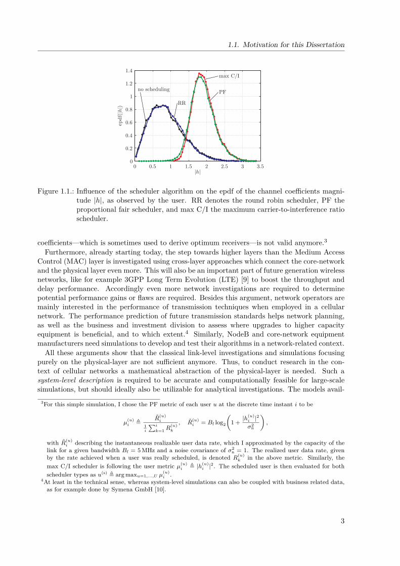
Figure 1.1 compares the influence of various types of schedulers (Round Robin (RR), Pro-portional Fair (PF) and Maximum Carrier-to-Interference Ratio (max C/I)) in terms of theempirical probability density function (epdf) of the magnitude of the channel epdf(|h|) as seenby the respectively scheduled user. It can be observed that the RR scheduler preserves theRayleigh distribution of |h|. Note however that this conclusion only holds because the individ-ual channels of the users are assumed to be statistically independent. In fact, when a moresophisticated scheduler that takes advantage of any available Channel State Information (CSI)is utilized, the situation changes dramatically. Both, the PF and the max C/I scheduler deformthe epdf significantly, which clearly shows that the assumption of Rayleigh distributed fading
2UMTS specifications define FDD and Time Division Duplex (TDD) operation modes, whereas in Europe mostlyFDD is used. Only in the Czech Republic TDD UMTS is deployed.
2
1.1. Motivation for this Dissertation
0 0.5 1 1.5 2 2.5 3 3.50
0.2
0.4
0.6
0.8
1
1.2
1.4
no scheduling
RR
max C/I
PF
Figure 1.1.: Influence of the scheduler algorithm on the epdf of the channel coefficients magni-tude |h|, as observed by the user. RR denotes the round robin scheduler, PF theproportional fair scheduler, and max C/I the maximum carrier-to-interference ratioscheduler.
coefficients—which is sometimes used to derive optimum receivers—is not valid anymore.3Furthermore, already starting today, the step towards higher layers than the Medium Access
Control (MAC) layer is investigated using cross-layer approaches which connect the core-networkand the physical layer even more. This will also be an important part of future generation wirelessnetworks, like for example 3GPP Long Term Evolution (LTE) [9] to boost the throughput anddelay performance. Accordingly even more network investigations are required to determinepotential performance gains or flaws are required. Besides this argument, network operators aremainly interested in the performance of transmission techniques when employed in a cellularnetwork. The performance prediction of future transmission standards helps network planning,as well as the business and investment division to assess where upgrades to higher capacityequipment is beneficial, and to which extent.4 Similarly, NodeB and core-network equipmentmanufacturers need simulations to develop and test their algorithms in a network-related context.
All these arguments show that the classical link-level investigations and simulations focusingpurely on the physical-layer are not sufficient anymore. Thus, to conduct research in the con-text of cellular networks a mathematical abstraction of the physical-layer is needed. Such asystem-level description is required to be accurate and computationally feasible for large-scalesimulations, but should ideally also be utilizable for analytical investigations. The models avail-
3For this simple simulation, I chose the PF metric of each user u at the discrete time instant i to be
µ(u)i ,
R(u)i
1i
∑i
k=1 R(u)k
, R(u)i = Bf log2
(1 + |h
(u)i |
2
σ2n
),
with R(u)i describing the instantaneous realizable user data rate, which I approximated by the capacity of the
link for a given bandwidth Bf = 5 MHz and a noise covariance of σ2n = 1. The realized user data rate, given
by the rate achieved when a user was really scheduled, is denoted R(u)k in the above metric. Similarly, the
max C/I scheduler is following the user metric µ(u)i , |h(u)
i |2. The scheduled user is then evaluated for both
scheduler types as u(s) , arg maxu=1,...,U µ(u)i .
4At least in the technical sense, whereas system-level simulations can also be coupled with business related data,as for example done by Symena GmbH [10].
3
Chapter 1. Introduction
able in literature do not cover MIMO HSDPA so far. Besides, many of them lack sufficientaccuracy, analytical applicability, or computational efficiency. The presented work is targeted toprovide a system-level description that solves these issues in a comprehensive way.
Importance of System-Level Optimization
The opportunities offered by the interaction of the lower layers and the MIMO extension ofHSDPA are very diverse. Unfortunately, most of the existing algorithms only exploit parts ofthese possibilities. Todays schedulers do not consider content-information, MIMO adaptationalgorithms work independent of global interference-minimization goals, and receivers treat thedownlink as single-user situation, to name a few.
Pressure on cost and the wish to exploit the full performance potential of the acquired hard-ware, however, requires close-to optimum network algorithms and transceiver structures. Mythesis is thus also aiming at improvements to some network algorithms as well as to the classicalMinimum Mean Squared Error (MMSE) equalizer structure.
1.2. Scope of Work and Contributions
As already outlined, the main objective of this thesis is the development and application of asuitable system-level description5 for the downlink of MIMO enhanced HSDPA, with particularfocus on the D-TxAA transmission mode. My proposed system-level model serves as a basis forthe concept of a system-level simulator and its implementation in a Matlab-environment. Thissimulator then builds a platform to investigate various parts of HSDPA networks.
Especially in packet-data-driven networks, like HSDPA, the system-level performance stronglydepends on the algorithms in use. As a matter of fact, the increased adaptability of the physicallayer can be utilized to fine-tune the network elements in order to realize potential gains or make itmore robust. To some extent, these approaches may also be considered to be cross-layer like [11],where information from higher layers may be utilized. With the Radio Link Control (RLC)being of main interest, I put the focus of my thesis on the downlink of HSDPA. The conductedinvestigations result in the development and testing of improved network-based algorithms. Thesealgorithms show substantial benefits compared to previously published methods.
Although this work addresses MIMO HSDPA, the basic methodology of the system-level mod-eling as well as the simulation concept may also be useful for future mobile communicationsystems. System-level analysis provides the necessary tools for the study and the developmentof such networks and their network-based—potentially cross-layer—algorithms.
In the following, the organization of this thesis in chapters and the novel contributions thereinare explained. Furthermore, the relevant original publications (co)-authored are cited and com-mented.
Chapter 2: HSDPA and its MIMO Enhancements
At the beginning, I review the basic properties of HSDPA and its MIMO-enhanced successor,D-TxAA HSDPA. I put a special focus on the aspects of the standards that play an importantrole in the context of my related investigations. The description explains the basic algorithmsof the core network and the wireless access scheme that define HSDPA compared to UMTS.
5An accurate definition of the term system-level description is provided in Chapter 3.
4
1.2. Scope of Work and Contributions
Also some of the most important aspects concerning the underlying MIMO principles on whichD-TxAA is build upon are elaborated.
Chapter 3: System-Level Modeling for MIMO Enhanced HSDPA
In this chapter, the concept of the proposed system-level modeling approach is introduced first,explaining the motivation and the basic constraints behind it, as well as its application in network-based research. I also elaborate on the difference between physical-layer, also called link-level,investigations and system-level based network studies, and discuss the advantages and limits ofboth aspects. Some of these findings have already been published in [12–14].
First, a computationally efficient link-quality model is developed, which analytically describesthe MIMO HSDPA link quality in the network context. The proposed model is very flexible indescribing various transmission setups, including even higher order spatial multiplexing schemesthan the standardized D-TxAA mode. Furthermore, the interference terms in the link-qualitymodel are described by means of so-called equivalent fading parameters, which can be evaluatedprior to the system-level simulation. This allows to dramatically reduce the computationalcomplexity needed during the runtime of the system-level simulation. The link-quality model isthen validated against link-level simulation results, showing an almost perfect approximation ofthe true Signal-to-Interference-and-Noise Ratio (SINR). By analytical analysis, I also identify afundamental performance limit of the D-TxAA Spatial Division Multiple Access (SDMA) user-separation capabilities, when utilizing the standard 3GPP pre-coding codebook. To highlightthe virtue of the proposed model, I elaborate on the modeling deficiencies of a pure statisticalapproach, and assess the computational complexity reduction in a semi-analytical framework.The core parts of the link-quality model were published in [12,13,15,16].
Second, my concept for the link-performance model which describes the BLock Error Ratio(BLER) performance of the system is presented. In principle, the model is composed of atransmission parameter adaptive mapping/compression of the link-quality model parametersand a successive Additive White Gaussian Noise (AWGN) based BLER performance prediction.Consecutively, the training of the link performance model, meaning the tuning of the parameterswithin the utilized compression/mapping description, is conducted. The necessary link-levelsimulations also serve to validate the link-performance model [14,17].
In short, the novel contributions to the area of system-level modeling research are:
• The proposed link-quality model provides an highly accurate description of the HSDPAlink-quality in the network context that has not been available before [12,15].
• The model uses equivalent fading parameters to render the effects of the channel, whichcan be calculated prior to the system-level simulation. This allows a huge reduction of thecomputational complexity during system-level simulation runtime [13,14].
• The link-performance model utilizes an established conceptual approach, but introducesthe idea of slot-based sampled compression/mapping in the Mutual Information (MI) do-main [14,17].
• In addition, the necessary training for the tuning parameters are conducted in the SINRdomain, which provides a good fit over the whole BLER region of interest [14,16].
Finally, let me point out that the developed link-quality model is currently used by NokiaSiemens Networks (NSN) in their packet-based system-level simulator Mobile Radio Simulation
5

Chapter 1. Introduction
Environment (MoRSE) where it serves as the core for the development and testing of base-station equipment and algorithms. The link-quality and the link-performance models have alsobeen utilized within the C 10 and C 12 projects [12, 17] conducted at ftw. in collaboration withInfineon AG.
Chapter 4: System-Level Simulation Based Optimization of MIMO Enhanced HSDPA
The proposed system-level model serves as the core for the development of a system-level sim-ulator. First, the concept of the system-level simulator including its advantages and limitationsis explained. Then, network performance prediction results from a set of D-TxAA system-levelsimulations are presented and discussed. I relate the obtained statistics of the average userthroughput to fairness measures and compare different network setups by means of their averageand maximum sector throughputs. I also shortly discuss the consequences of the double-streamoperation onto the fairness in the network. Some of these results have been published in [14].
Consecutively, a novel RLC-based stream number decision algorithm with enhanced robustnessagainst signaling errors from the UE side is proposed [18]. The system-level simulator is alsoutilized to conduct performance evaluations of an optimized cross-layer scheduler. Also theachievable Quality of Experience (QoE) gains in an HSDPA network [19, 20] are investigated.Finally, by extending the proposed system-level model, Common Pilot CHannel (CPICH) poweroptimizations for various antenna configurations are performed [21]. The presented results givethe optimum average CPICH power values maximizing the HSDPA link-quality.
The findings presented in this chapter can be summarized as follows:
• A flexible system-level simulator concept suitable for performance analysis and algorithmtesting in the MAC layer is proposed [14].• New MIMO HSDPA network performance results including guidelines for the network
planing are derived [14].• A robust RLC stream number decision algorithm, residing in the NodeB is developed. The
algorithm is able to outperform UE based stream number determining in case of shortchannel coherence time [18].• A novel cross-layer content-aware scheduler exploiting information about the physical-layer
link-quality to increase the QoE for streamed videos in an HSDPA network is proposed [19,20].• Optimum CPICH power values for various antenna deployments, channel characteristics,
and MIMO transmission modes are evaluated [21].
Chapter 5: Multi-User MMSE Equalization for MIMO Enhanced HSDPA
The previous chapters were based on the assumption of a classical single-user MMSE receiver.In Chapter 5, however, I investigate the structure of the intra-cell interference when multipleusers are simultaneously active. In fact, the special form of the interference imposed by themulti-user Transmit Antenna Array (TxAA) transmission requires an enhanced system modelto derive an interference-aware MMSE equalizer. The proposed equalizer takes the pre-codingstate of the cell into account. By means of system-level analysis, I investigate the interferencesuppression capabilities and the theoretical performance limits of the developed receiver whenperfect knowledge of the pre-coding state is available [17, 22, 23]. In a practical setup, however,only the pre-coding information of the desired user is known. The basic principle applied to
6
1.2. Scope of Work and Contributions
derive a suitable blind estimator is the Gaussian Maximum Likelihood (ML) approach. Somesemi-analytical results on the complexity order of the interference-aware equalizer and the pre-coding state estimator also show that the overall complexity increase is only moderate [24].
Finally, physical-layer and system-level simulations are performed that show significant through-put performance gains of the interference-aware MMSE equalizer compared to the classical single-user MMSE equalizer [25].
In short, the main contributions of this chapter are:
• A system model representing the TxAA multi-user interference structure is presented, thecorresponding MMSE equalizer is derived, and its theoretical limits are investigated [17,22,23].• A training-based and a blind pre-coding state estimator are developed and their perfor-
mances are compared [25].• Physical-layer and system-level simulation results show the large throughput performance
gain of the proposed interference-aware MMSE equalizer [24,25].
Chapter 6: Conclusions
Chapter 6 concludes the main part of my thesis. The contributions and implications of mypresented work are discussed. I also elaborate on the lessons learned and give an outlook onpossible further research.
Appendix A: Additional Informative Material
The first appendix combines additional information and details on the explanations in the mainchapters of the thesis. I give further information on some of the HSDPA concepts that are notnecessarily needed for the expert in the context of the presented work, but still lead to a betterunderstanding of the subject. Details on the assumptions, theorems, and algorithms referencedand utilized in the main part of the thesis are also discussed. Additional simulation results forsome of the findings in the main part round off the information presented in this chapter.
Appendix B: Further System-Level Modeling, Simulations, Optimizations, and Validation
The main part of this thesis addresses MIMO HSDPA. However, currently SISO HSDPA isstill the standard deployed in wireless networks. Thus, this appendix presents some system-levelresearch for SISO HSDPA [26] that I have conducted as part of a cooperation with mobilkomaustria AG.
Furthermore, some of the signaling channels of HSDPA are allowed to utilize Space-TimeTransmit Diversity (STTD) schemes. Thus a link-quality model based on Alamouti encodedtransmission is studied here [15]. These findings are not necessary for the work in the main partof the thesis. Nevertheless they might be useful for future extended system-level simulations.
7

Chapter 2.
HSDPA and its MIMO EnhancementsHowever far modern science andtechniques have fallen short of theirinherent possibilities, they havetaught mankind at least one lesson:Nothing is impossible.
(Lewis Mumford)
Radio access evolution attempts to enable the smooth usage of modern applications in wire-less telecommunication networks. Since the introduction of the Global System for Mobile
communications (GSM) in 1991, the ecosystem of equipment vendors, application providers andservice enablers has grown significantly. Moreover, the development and availability of wirelessbroadband techniques now allows for an even tighter integration of web-based services on mobiledevices. In the context of wireless networks, the key parameters defining the application perfor-mance include the data rate and the network latency. Some applications require only low bitrates of a few tens of kbit/s but demand very low delay, like Voice over IP (VoIP) and onlinegames [27]. On the other hand, the download time of large files is only defined by the maximumdata rate, and latency does not play a big role.
In terms of penetration, mobile wireless telephony has passed the fixed line volumes already in2004, whereas the broadband coverage is still lacking behind [28]. However, the mobile broadband(data cards) penetration rate for example in Austria has now (2009) reached 11.4 % [29]. Currentsurveys forecast a maximum penetration of approximately 25 % for European markets [30].1HSDPA playes a big, if not the most important role in the success of mobile broadband services.The dramatic push of the typical data rates, as well as the achievable peak data rate compared toUMTS together with the lowered latency received a lot of attention from customers. In addition,the rapid decline in prices [31] and the low cost hardware to connect conveniently to HSDPAnetworks are very attractive for the end users. Nowadays, no or only little effort is required toadapt Internet applications to the mobile environment.
Essentially, HSDPA for the first time offers a broadband wireless access with seamless mobil-ity and extensive coverage. Together with High-Speed Uplink Packet Access (HSUPA), HSDPAforms the so-called High-Speed Packet Access (HSPA), which can be deployed on top of theexisting WCDMA UMTS networks, either on the same carrier,2 or—for high capacity and highbit rate—on another carrier thus consequently denoting a pure HSDPA operation. The ever in-creasing demand for HSDPA broadband wireless access however drives mobile network operatorsto allocate their spectrum resources in a progressive way towards HSPA usage.
1In Indonesia actually, HSDPA broadband access passed the fixed broadband access in 2008!2This requires the split of the spreading code resources in the cell.
9
Chapter 2. HSDPA and its MIMO Enhancements
Terminal
NodeB Drift RNC ServingRNC
Core Network
Internet
Uu Iub Iur Iu
IPPDCPRLC
MAC-d
MAC-hsWCDMA L1
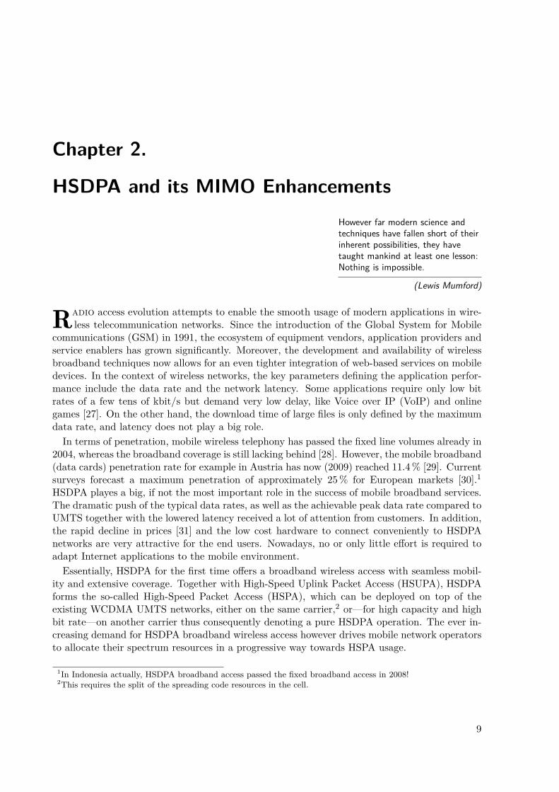
Figure 2.1.: Network architecture for HSDPA including the protocol gateways.
2.1. HSDPA Principles
The introduction of HSDPA in the 3GPP Release 5 implied a number of changes in the wholesystem architecture. As a matter of fact, not only the terminal but also the NodeB and theRadio Network Controller (RNC) were affected [32].
2.1.1. Network Architecture
The principal network architecture for the operation of HSDPA is still equal to the architecturefor UMTS networks [3], see Figure 2.1. Basically, the network can be split in three parts, (i)the UE or terminal connected via the Uu interface, (ii) the Universal mobile telecommunicationssystem Terrestrial Radio Access Network (UTRAN), including everything from the NodeB tothe serving RNC, and (iii) the core network, connected via the Iu interface, that establishes thelink to the internet. Within the UTRAN, several NodeBs—each of which can control multiplesectors3—are connected to the drift RNC via the Iub interface. This intermediate RNC is neededfor the soft handover functionality in Release 99, and is also formally supported by HSDPA.However, for HSDPA, soft handover has been discarded, thus eliminating the need to run userdata over multiple Iub and Iur interfaces to connect the NodeB with the drift RNCs and theserving RNC. This also implies that the HSDPA UE is only attached to one NodeB, and in caseof mobility a hard-handover between different NodeBs is necessary. In conclusion, the typicalHSDPA scenario could be represented by just one single RNC [33], allowing me to treat it as asingle RNC in this work.
For the HSDPA operation, the NodeB has to handle downlink scheduling, dynamic resource al-location, Quality of Service (QoS) provisioning, load and overload control, fast Hybrid AutomaticRepeat reQuest (HARQ) retransmission handling, as well as the physical layer processing itself.The drift RNC on the other hand performs the layer two processing and keeps control over theradio resource reservation for HSDPA, downlink code allocation and code tree handling, overallload and overload control, as well as admission control. Finally, the serving RNC is responsiblefor the QoS parameters mapping and handover control.
The buffer in the NodeB in cooperation with the scheduler enables having a higher peak datarate for the radio interface Uu than the average rate on the Iub. For 7.2 Mbit/s terminal devices,
3In this work, I use the following terminology: a NodeB (that means base-station, or site) contains multiple cells(that means sectors) in a sectored network.
10

2.1. HSDPA Principles
Application Layer(Encoder)
RTPReal-Time Transport Protocol
UDPUser Datagram Protocol
IPInternet Protocol
RLCRadio Link Control
MAC-hs
PHYPhysical Layer
MAC-c/sh
MAC-d
PDCPPaket Data Convergence Protocol
Application side
Core-Network transport
Gateway
Physical layercoordination
Wireless transmissionhandling
Figure 2.2.: Protocol design in UMTS from the application to the physical layer.
the Iub connection speed can somewhere be chosen around 1 Mbit/s [33]. With the transmissionbuffer in the NodeB, the flow control has to take care to avoid potential buffer overflows.
In the core network, the Internet Protocol (IP) plays the dominant role for packet-switchedinterworking. On the UTRAN side, the headers of the IP packets are compressed by the PacketData Convergence Protocol (PDCP) protocol to improve the efficiency of small packet transmis-sions, for example VoIP. The RLC protocol handles the segmentation and retransmission for bothuser and control data. For HSDPA the RLC may be operated either (i) in unacknowledged mode,when no RLC layer retransmission will take place, or (ii) in acknowledged mode, so that datadelivery is ensured. The MAC layer functionalities of UMTS have been broadened for HSDPA,in particular a new MAC protocol entity, the Medium Access Control for High-Speed DownlinkPacket Access (MAC-hs) has been introduced in the NodeB. Now, the MAC layer functionalitiesof HSDPA can operate independently of UMTS, but take the overall resource limitations in theair into account. The RNC retains the Medium Access Control dedicated (MAC-d) protocol, butthe only remaining functionality is the transport channel switching. All other functionalities,such as scheduling and priority handling, are moved to the MAC-hs. Figure 2.2 illustrates thestack of protocols in UMTS based networks including their purpose.
For the operation of HSDPA, new transport channels and new physical channels have beendefined. Figure 2.3 shows the physical channels as employed between the NodeB and the UE, aswell as their connection to the utilized transport channels and logical channels [34]. The physicalchannels correspond in this context to the layer one of the Open Systems Interconnection (OSI)model, with each of them being defined by a specific carrier frequency, scrambling code, spreadingcode,4 as well as start and stop timing. For the communication to the MAC layer, the physicalchannels are combined into the so-called transport channels. In HSDPA operated networks,only two transport channels are needed, (i) the High-Speed Downlink Shared CHannel (HS-
4Also called channelization code.
11
Chapter 2. HSDPA and its MIMO Enhancements
HS-PDSCH
HS-SCCHHS-DPCCH
DPDCH, DPCCHNodeB Terminal
Logical channels Transport channels Physical channels
DTCH
DCCH
HS-DSCH
DCH
HS-PDSCH
HS-SCCH
HS-DPCCH
DPDCH
DPCCH
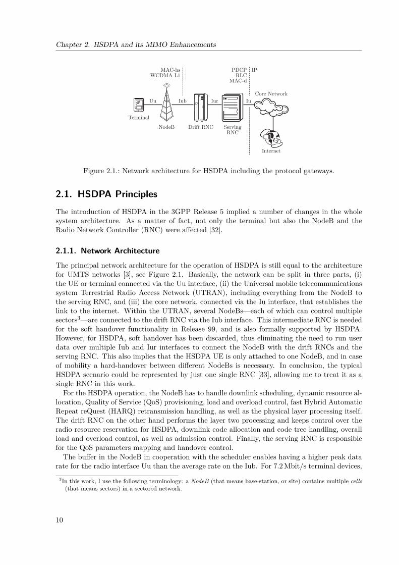
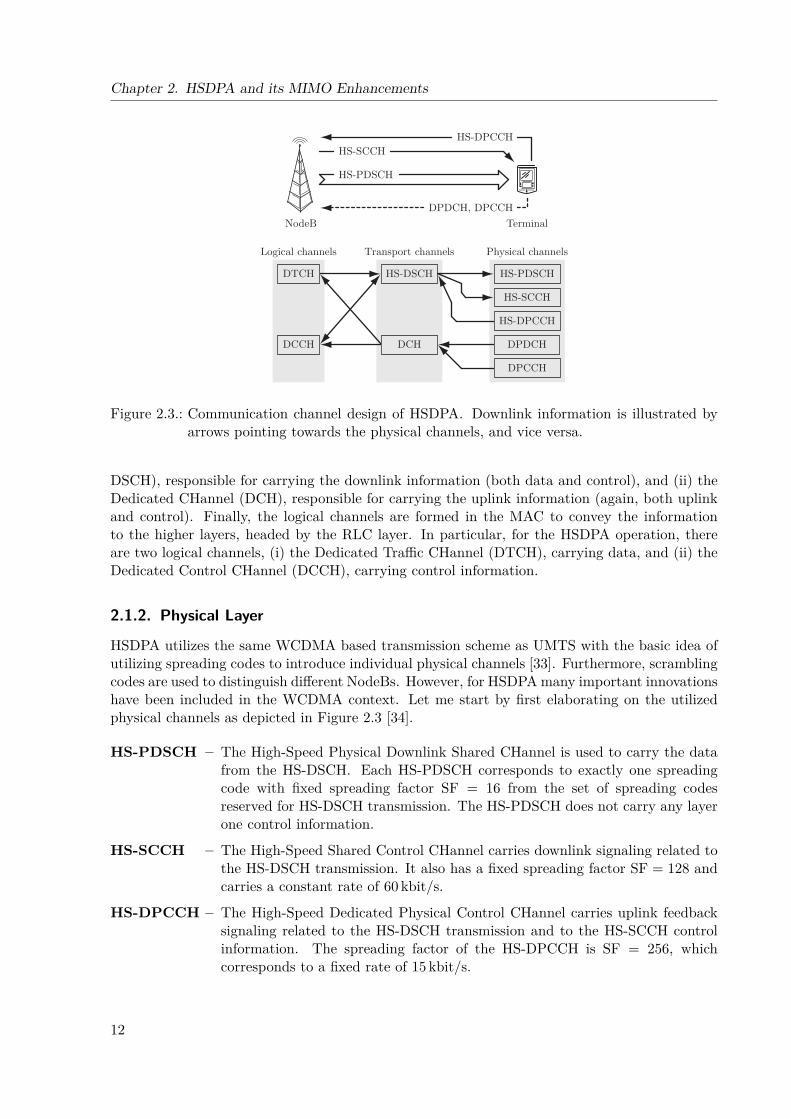
Figure 2.3.: Communication channel design of HSDPA. Downlink information is illustrated byarrows pointing towards the physical channels, and vice versa.
DSCH), responsible for carrying the downlink information (both data and control), and (ii) theDedicated CHannel (DCH), responsible for carrying the uplink information (again, both uplinkand control). Finally, the logical channels are formed in the MAC to convey the informationto the higher layers, headed by the RLC layer. In particular, for the HSDPA operation, thereare two logical channels, (i) the Dedicated Traffic CHannel (DTCH), carrying data, and (ii) theDedicated Control CHannel (DCCH), carrying control information.
2.1.2. Physical Layer
HSDPA utilizes the same WCDMA based transmission scheme as UMTS with the basic idea ofutilizing spreading codes to introduce individual physical channels [33]. Furthermore, scramblingcodes are used to distinguish different NodeBs. However, for HSDPA many important innovationshave been included in the WCDMA context. Let me start by first elaborating on the utilizedphysical channels as depicted in Figure 2.3 [34].
HS-PDSCH – The High-Speed Physical Downlink Shared CHannel is used to carry the datafrom the HS-DSCH. Each HS-PDSCH corresponds to exactly one spreadingcode with fixed spreading factor SF = 16 from the set of spreading codesreserved for HS-DSCH transmission. The HS-PDSCH does not carry any layerone control information.
HS-SCCH – The High-Speed Shared Control CHannel carries downlink signaling related tothe HS-DSCH transmission. It also has a fixed spreading factor SF = 128 andcarries a constant rate of 60 kbit/s.
HS-DPCCH – The High-Speed Dedicated Physical Control CHannel carries uplink feedbacksignaling related to the HS-DSCH transmission and to the HS-SCCH controlinformation. The spreading factor of the HS-DPCCH is SF = 256, whichcorresponds to a fixed rate of 15 kbit/s.
12
2.1. HSDPA Principles
DPDCH – The Dedicated Physical Data CHannel is used to carry the uplink data of theDCH transport channel. There may be more than one DPDCH on the uplink,with the spreading factor ranging from SF = 256 down to SF = 4.
DPCCH – The Dedicated Physical Control CHannel carries the layer one control informa-tion associated to the DPDCH. The layer one control information consists ofknown pilot bits to support channel estimation for coherent detection, Trans-mit Power-Control (TPC) commands, FeedBack Information (FBI), and an op-tional Transport-Format Combination Indicator (TFCI). The DPCCH utilizesa spreading factor of SF = 256, which corresponds to a fixed rate of 15 kbit/s.
In WCDMA, thus also in HSDPA, timing relations are denoted in terms of multiple of chips.In the 3GPP specifications, suitable multiples of the chips are: (i) a radio frame which is theprocessing duration of 38 400 chips,5 corresponding to a duration of 10 ms, (ii) a slot consistingof 2 560 chips, thus defining a radio frame to comprise 15 slots, and (iii) a sub-frame, whichcorresponds to three slots or 7 560 chips, which is also called Transmission Time Interval (TTI),because it defines the basic timing interval for the HS-DSCH transmission of one transport block.
The general HSDPA operation principle brings a new paradigm in the dynamical adaptationto the channel as utilized in UMTS. Formerly relying on the fast power control [3], now theNodeB obtains information about the channel quality of each active HSDPA user on the basisof physical layer feedback, denoted CQI [7]. Link adaptation is then performed by means ofAdaptive Modulation and Coding (AMC), which allows for an increased dynamic range comparedto the possibilities of the fast power control. The transport format used by the AMC, that ismodulation alphabet size and effective channel coding rate, is chosen to achieve a chosen targetBLER.6 Now one may ask why a system should be operated at an error rate that is boundabove zero. Two main arguments for this basic ideology of link adaptation is that (i) in practicalsystems the UE has to inform the network about the correct or incorrect reception of a packet.Since this information is needed to guarantee a reliable data transmission, it makes no sense topush the error probability of the data channel lower than the error rate of the signaling channel.Furthermore, by fixing the BLER to a given value, (ii) the link adaptation has the possibility toremove outage events of the channel.
On top of the link adaptation in terms of the modulation alphabet size and the effective codingrate, HSDPA can take excessive use of the multi-code operation, up to the full spreading coderesource allocation in a cell. The other new key technology is the physical-layer retransmission.Whereas in UMTS retransmissions are handled by the RNC, in HSDPA the NodeB buffers theincoming packets and in case of decoding failure, retransmission automatically takes place fromthe base station, without RNC involvement. Should the physical layer operation fail, then RNCbased retransmission may still be applied on top. Finally, as already mentioned, the NodeB nowis in charge of the scheduling and resource allocation. Table 2.1 summarizes the key differencesbetween UMTS and HSDPA [33].
HSDPA User Data Transmission
Together with the various new features as listed in Table 2.1, Release 5 HSDPA also came alongwith the support of higher order modulation, in particular 16 QAM. This made it necessary thatnot only the phase has to be estimated correctly—as in the UMTS case—but also the amplitude
5In the 3GPP WCDMA systems, the chip rate is fixed at 3.84 Mchips/s, utilizing a bandwidth of 5 MHz.6One block denotes one TTI in HSDPA.
13
Chapter 2. HSDPA and its MIMO Enhancements
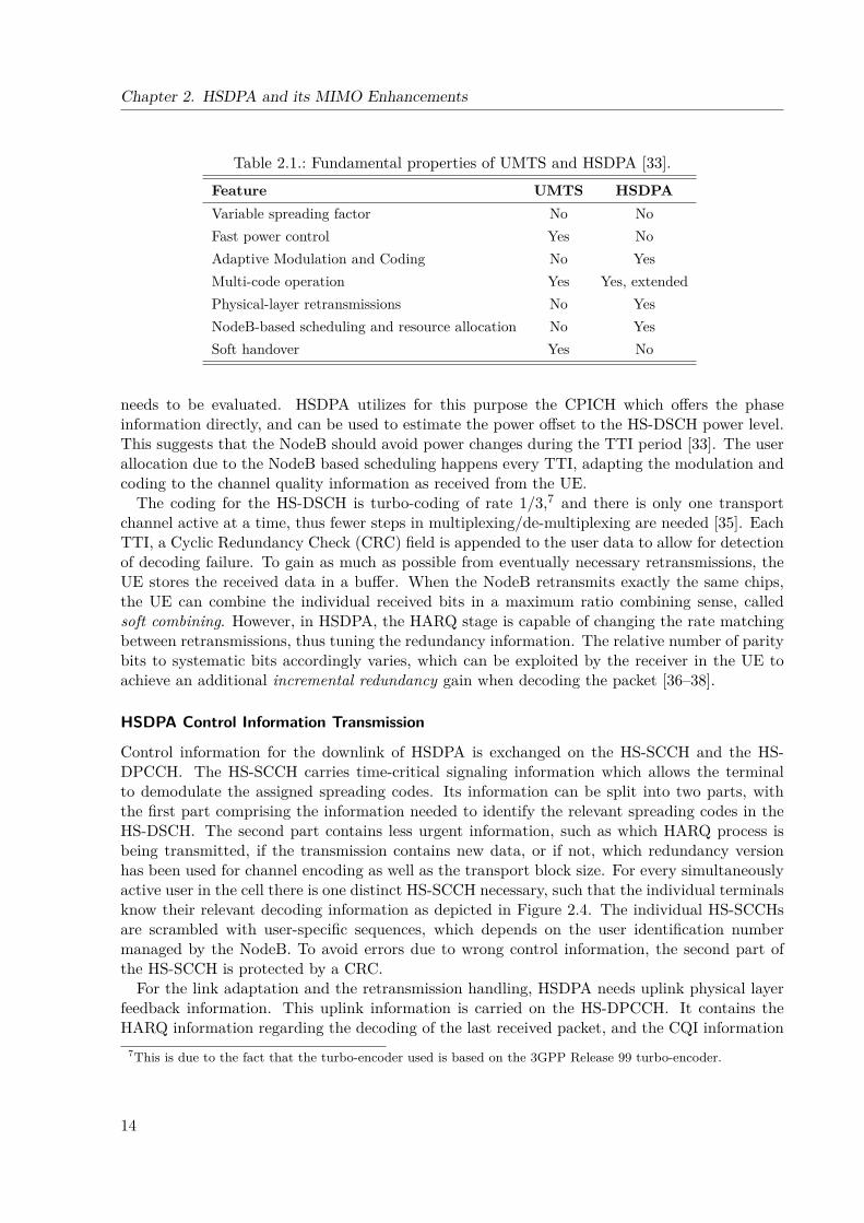
Table 2.1.: Fundamental properties of UMTS and HSDPA [33].Feature UMTS HSDPAVariable spreading factor No NoFast power control Yes NoAdaptive Modulation and Coding No YesMulti-code operation Yes Yes, extendedPhysical-layer retransmissions No YesNodeB-based scheduling and resource allocation No YesSoft handover Yes No
needs to be evaluated. HSDPA utilizes for this purpose the CPICH which offers the phaseinformation directly, and can be used to estimate the power offset to the HS-DSCH power level.This suggests that the NodeB should avoid power changes during the TTI period [33]. The userallocation due to the NodeB based scheduling happens every TTI, adapting the modulation andcoding to the channel quality information as received from the UE.
The coding for the HS-DSCH is turbo-coding of rate 1/3,7 and there is only one transportchannel active at a time, thus fewer steps in multiplexing/de-multiplexing are needed [35]. EachTTI, a Cyclic Redundancy Check (CRC) field is appended to the user data to allow for detectionof decoding failure. To gain as much as possible from eventually necessary retransmissions, theUE stores the received data in a buffer. When the NodeB retransmits exactly the same chips,the UE can combine the individual received bits in a maximum ratio combining sense, calledsoft combining. However, in HSDPA, the HARQ stage is capable of changing the rate matchingbetween retransmissions, thus tuning the redundancy information. The relative number of paritybits to systematic bits accordingly varies, which can be exploited by the receiver in the UE toachieve an additional incremental redundancy gain when decoding the packet [36–38].
HSDPA Control Information Transmission
Control information for the downlink of HSDPA is exchanged on the HS-SCCH and the HS-DPCCH. The HS-SCCH carries time-critical signaling information which allows the terminalto demodulate the assigned spreading codes. Its information can be split into two parts, withthe first part comprising the information needed to identify the relevant spreading codes in theHS-DSCH. The second part contains less urgent information, such as which HARQ process isbeing transmitted, if the transmission contains new data, or if not, which redundancy versionhas been used for channel encoding as well as the transport block size. For every simultaneouslyactive user in the cell there is one distinct HS-SCCH necessary, such that the individual terminalsknow their relevant decoding information as depicted in Figure 2.4. The individual HS-SCCHsare scrambled with user-specific sequences, which depends on the user identification numbermanaged by the NodeB. To avoid errors due to wrong control information, the second part ofthe HS-SCCH is protected by a CRC.
For the link adaptation and the retransmission handling, HSDPA needs uplink physical layerfeedback information. This uplink information is carried on the HS-DPCCH. It contains theHARQ information regarding the decoding of the last received packet, and the CQI information
7This is due to the fact that the turbo-encoder used is based on the 3GPP Release 99 turbo-encoder.
14
2.1. HSDPA Principles
HS-SCCH user 1
HS-SCCH user 2
HS-DSCH 1 TTI
decodinginformation
8 HS-PDSCH
HS-PDSCH 1
1 TTI fullyallocated to user 2
3 HS-PDSCHallocated to user 1
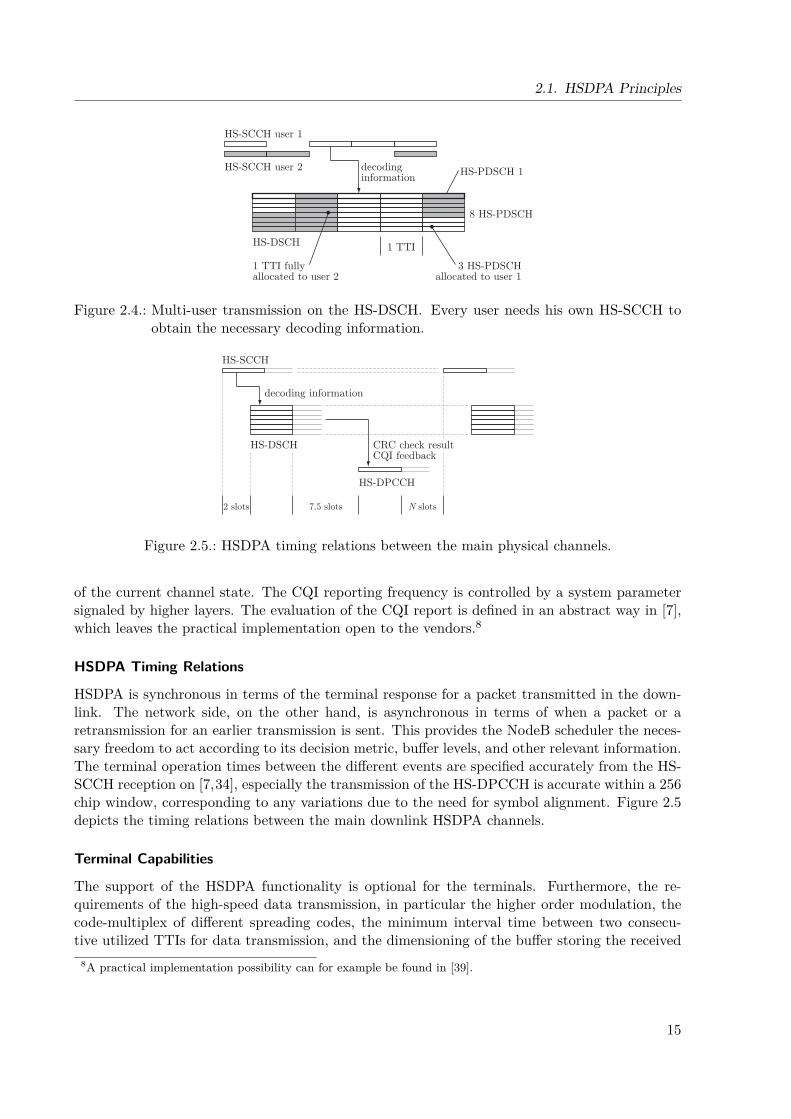
Figure 2.4.: Multi-user transmission on the HS-DSCH. Every user needs his own HS-SCCH toobtain the necessary decoding information.
HS-SCCH
HS-DSCH
HS-DPCCH
decoding information
CRC check resultCQI feedback
2 slots 7.5 slots N slots
Figure 2.5.: HSDPA timing relations between the main physical channels.
of the current channel state. The CQI reporting frequency is controlled by a system parametersignaled by higher layers. The evaluation of the CQI report is defined in an abstract way in [7],which leaves the practical implementation open to the vendors.8
HSDPA Timing Relations
HSDPA is synchronous in terms of the terminal response for a packet transmitted in the down-link. The network side, on the other hand, is asynchronous in terms of when a packet or aretransmission for an earlier transmission is sent. This provides the NodeB scheduler the neces-sary freedom to act according to its decision metric, buffer levels, and other relevant information.The terminal operation times between the different events are specified accurately from the HS-SCCH reception on [7,34], especially the transmission of the HS-DPCCH is accurate within a 256chip window, corresponding to any variations due to the need for symbol alignment. Figure 2.5depicts the timing relations between the main downlink HSDPA channels.
Terminal Capabilities
The support of the HSDPA functionality is optional for the terminals. Furthermore, the re-quirements of the high-speed data transmission, in particular the higher order modulation, thecode-multiplex of different spreading codes, the minimum interval time between two consecu-tive utilized TTIs for data transmission, and the dimensioning of the buffer storing the received
8A practical implementation possibility can for example be found in [39].
15
Chapter 2. HSDPA and its MIMO Enhancements
samples for retransmission combining put tough constraints on the equipment. Accordingly, the3GPP defined twelve UE capability classes effectively specifying the maximum throughput thatcan be handled by the device [7, 40]. The highest capability is provided by category ten, whichallows the theoretical maximum data rate of 14.4 Mbit/s. This rate is achievable with one-thirdrate turbo coding and significant puncturing,9 resulting in a code rate close to one. For a list ofterminal capability classes, see for example [33].
2.1.3. MAC Layer
The HSDPA MAC layer comprises three key functionalities: (i) the scheduling, (ii) the HARQretransmission handling, and (iii) the link adaptation, respectively resource allocation [41]. Notethat the 3GPP specifications do not contain any parameters for the scheduler operation, whichis left open for individual implementation to the vendors. Similar arguments hold for the othertwo functionalities, with the exception that (ii) and (iii) have to obey more stringent restrictionsdue to the interworking with the UE side.
For the operation of the HARQ retransmissions, the MAC-hs layer has to consider some im-portant points. To avoid wasting time between transmission of the data block and reception ofthe ACKnowledged (ACK)/Non-ACKnowledged (NACK) response, which would result in low-ered throughput, multiple independent HARQ processes can be run in parallel within one HARQentity. The algorithm in use for this behavior is an N Stop And Wait (N-SAW) algorithm [42].However, the retransmission handling has to be aware of the UE minimum inter-TTI interval forreceiving data, which depends on the UE capability class.
The terminal is signaled some MAC layer parameters, with the MAC-hs Packet Data Unit(PDU) consisting of the MAC-hs header and the MAC-hs payload. It is built by one or moreMAC-hs Service Data Units (SDUs) and potential padding if they do not fit the size of the trans-port block available. As the packets are not arriving in sequence after the MAC HARQ operation,the terminal MAC layer has to cope with the packet reordering. The MAC header therefore in-cludes a Transmission Sequence Number (TSN) and a Size Index Identifier (SID) that revealsthe MAC-d PDU size and the number of MAC PDUs of the size indicated by the SID.
The MAC-d is capable of distinguishing between different services by means of MAC-d flows,each of which can have different QoS settings assigned. In the MAC-hs, every MAC-d flowobtains its own queue, to allow different reordering queues at the UE end. Note however thatonly one transport channel may exist in a single TTI and thus, in a single MAC-hs PDU. Thismeans that flows from different services can only be scheduled in consecutive TTIs [33,42].
2.1.4. Radio Resource Management
The Radio Resource Management (RRM) algorithms are responsible for transferring the physicallayer enhancements of HSDPA to capacity gain while providing attractive end user performanceand system stability. At the RNC, the HSDPA related algorithms include physical resourceallocation, admission control and mobility management. On the NodeB side, RRM includesHS-DSCH link adaptation, the already explained packer scheduler and HS-SCCH power control.
In order for the NodeB to transmit data on the HS-DSCH, the controlling RNC needs toallocate channelization codes and power for the transmission. As a minimum, one HS-SCCHcode and one HS-PDSCH code have to be assigned to the NodeB. The communication betweenthe RNC and the NodeB follows the NodeB Application Part (NBAP) protocol [43]. In case
9Puncturing is performed in the rate-matching stage.
16
2.1. HSDPA Principles
time time
power allocation power allocation
max. NodeB power
HSDPA power
non-HSDPA powernon-HSDPA power
safety marginHSDPA power
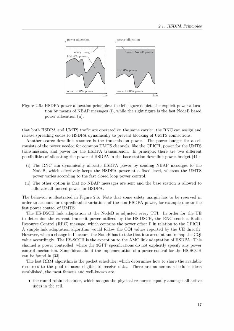
Figure 2.6.: HSDPA power allocation principles: the left figure depicts the explicit power alloca-tion by means of NBAP messages (i), while the right figure is the fast NodeB basedpower allocation (ii).
that both HSDPA and UMTS traffic are operated on the same carrier, the RNC can assign andrelease spreading codes to HSDPA dynamically to prevent blocking of UMTS connections.
Another scarce downlink resource is the transmission power. The power budget for a cellconsists of the power needed for common UMTS channels, like the CPICH, power for the UMTStransmissions, and power for the HSDPA transmission. In principle, there are two differentpossibilities of allocating the power of HSDPA in the base station downlink power budget [44]:
(i) The RNC can dynamically allocate HSDPA power by sending NBAP messages to theNodeB, which effectively keeps the HSDPA power at a fixed level, whereas the UMTSpower varies according to the fast closed loop power control.
(ii) The other option is that no NBAP messages are sent and the base station is allowed toallocate all unused power for HSDPA.
The behavior is illustrated in Figure 2.6. Note that some safety margin has to be reserved inorder to account for unpredictable variations of the non-HSDPA power, for example due to thefast power control of UMTS.
The HS-DSCH link adaptation at the NodeB is adjusted every TTI. In order for the UEto determine the current transmit power utilized by the HS-DSCH, the RNC sends a RadioResource Control (RRC) message, which contains the power offset Γ in relation to the CPICH.A simple link adaptation algorithm would follow the CQI values reported by the UE directly.However, when a change in Γ occurs, the NodeB has to take that into account and remap the CQIvalue accordingly. The HS-SCCH is the exception to the AMC link adaptation of HSDPA. Thischannel is power controlled, where the 3GPP specifications do not explicitly specify any powercontrol mechanism. Some ideas about the implementation of a power control for the HS-SCCHcan be found in [33].
The last RRM algorithm is the packet scheduler, which determines how to share the availableresources to the pool of users eligible to receive data. There are numerous scheduler ideasestablished, the most famous and well-known are
• the round robin scheduler, which assigns the physical resources equally amongst all activeusers in the cell,
17
Chapter 2. HSDPA and its MIMO Enhancements
• the maximum carrier-to-interference ratio scheduler, which assigns the physical resourcesto the user with the best carrier-to-interference ratio in order to maximize the cell through-put,10 and• the proportional fair scheduler trying to balance between throughput maximization and
fairness.11
Besides these allocation strategies, the scheduler can schedule multiple users within one TTI. Upto 15 HS-PDSCH may be used by the NodeB, which gives the scheduler the freedom to maximizespectral efficiency when scheduling more than one user at once. On the other hand, the schedulermay require a multi-user policy, if there are many HSDPA users that require a low source datarate but strict upper bounds on the delay, like for example VoIP.
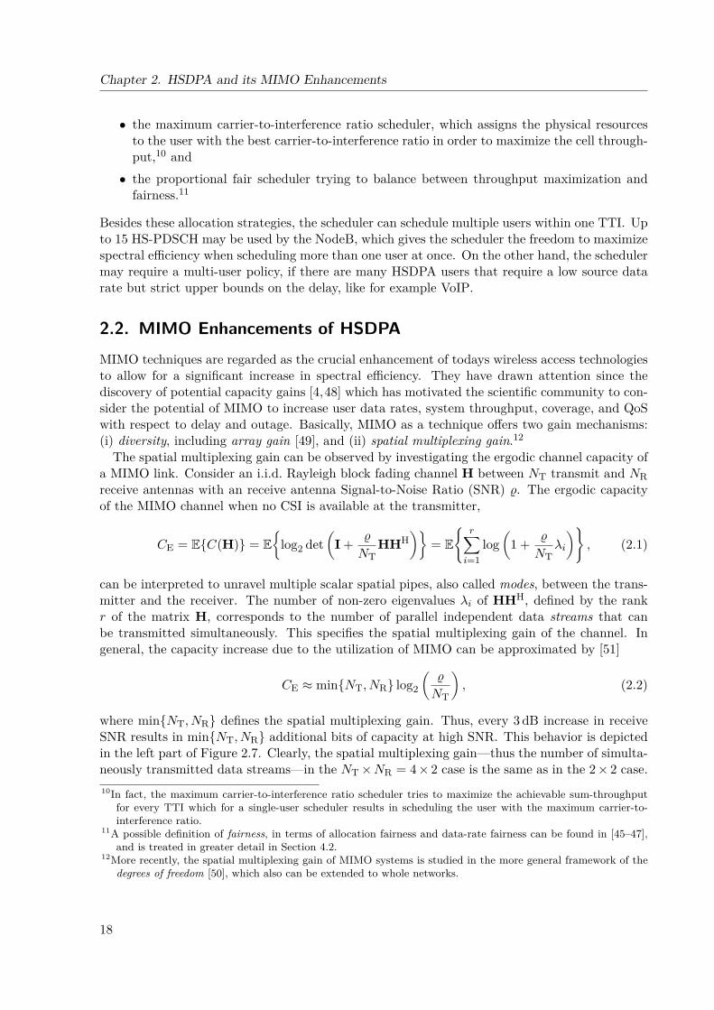
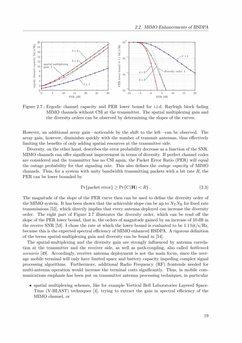
2.2. MIMO Enhancements of HSDPAMIMO techniques are regarded as the crucial enhancement of todays wireless access technologiesto allow for a significant increase in spectral efficiency. They have drawn attention since thediscovery of potential capacity gains [4,48] which has motivated the scientific community to con-sider the potential of MIMO to increase user data rates, system throughput, coverage, and QoSwith respect to delay and outage. Basically, MIMO as a technique offers two gain mechanisms:(i) diversity, including array gain [49], and (ii) spatial multiplexing gain.12
The spatial multiplexing gain can be observed by investigating the ergodic channel capacity ofa MIMO link. Consider an i.i.d. Rayleigh block fading channel H between NT transmit and NRreceive antennas with an receive antenna Signal-to-Noise Ratio (SNR) %. The ergodic capacityof the MIMO channel when no CSI is available at the transmitter,
CE = EC(H) = E
log2 det(
I + %
NTHHH
)= E
r∑i=1
log(
1 + %
NTλi
), (2.1)
can be interpreted to unravel multiple scalar spatial pipes, also called modes, between the trans-mitter and the receiver. The number of non-zero eigenvalues λi of HHH, defined by the rankr of the matrix H, corresponds to the number of parallel independent data streams that canbe transmitted simultaneously. This specifies the spatial multiplexing gain of the channel. Ingeneral, the capacity increase due to the utilization of MIMO can be approximated by [51]
CE ≈ minNT, NR log2
(%
NT
), (2.2)
where minNT, NR defines the spatial multiplexing gain. Thus, every 3 dB increase in receiveSNR results in minNT, NR additional bits of capacity at high SNR. This behavior is depictedin the left part of Figure 2.7. Clearly, the spatial multiplexing gain—thus the number of simulta-neously transmitted data streams—in the NT×NR = 4× 2 case is the same as in the 2× 2 case.10In fact, the maximum carrier-to-interference ratio scheduler tries to maximize the achievable sum-throughput
for every TTI which for a single-user scheduler results in scheduling the user with the maximum carrier-to-interference ratio.
11A possible definition of fairness, in terms of allocation fairness and data-rate fairness can be found in [45–47],and is treated in greater detail in Section 4.2.
12More recently, the spatial multiplexing gain of MIMO systems is studied in the more general framework of thedegrees of freedom [50], which also can be extended to whole networks.
18
2.2. MIMO Enhancements of HSDPA
0 5 10 15 20 25 300
2
4
6
8
10
12
14
16
18
20
SNR [dB]
ergo
dic
chan
nel ca
paci
ty [bi
t/s/
Hz]
−10 −5 0 5 10 15 2010
−3
10−2
10−1
100
SNR [dB]
PE
R low
er b
ound
@ 1
.1 b
it/s
/Hz
spatial multiplexinggain: 2
diversity order: 4
Figure 2.7.: Ergodic channel capacity and PER lower bound for i.i.d. Rayleigh block fadingMIMO channels without CSI at the transmitter. The spatial multiplexing gain andthe diversity orders can be observed by determining the slopes of the curves.
However, an additional array gain—noticeable by the shift to the left—can be observed. Thearray gain, however, diminishes quickly with the number of transmit antennas, thus effectivelylimiting the benefits of only adding spatial resources at the transmitter side.
Diversity, on the other hand, describes the error probability decrease as a function of the SNR.MIMO channels can offer significant improvement in terms of diversity. If perfect channel codesare considered and the transmitter has no CSI again, the Packet Error Ratio (PER) will equalthe outage probability for that signaling rate. This also defines the outage capacity of MIMOchannels. Thus, for a system with unity bandwidth transmitting packets with a bit rate R, thePER can be lower bounded by
Prpacket error ≥ PrC(H) < R . (2.3)
The magnitude of the slope of the PER curve then can be used to define the diversity order ofthe MIMO system. It has been shown that the achievable slope can be up to NTNR for fixed ratetransmissions [52], which directly implies that every antenna deployed can increase the diversityorder. The right part of Figure 2.7 illustrates the diversity order, which can be read off theslope of the PER lower bound, that is, the orders of magnitude gained by an increase of 10 dB inthe receive SNR [53]. I chose the rate at which the lower bound is evaluated to be 1.1 bit/s/Hz,because this is the expected spectral efficiency of MIMO enhanced HSDPA. A rigorous definitionof the terms spatial-multiplexing gain and diversity can be found in [54].
The spatial-multiplexing and the diversity gain are strongly influenced by antenna correla-tion at the transmitter and the receiver side, as well as path-coupling, also called bottleneckscenario [49]. Accordingly, receiver antenna deployment is not the main focus, since the aver-age mobile terminal will only have limited space and battery capacity impeding complex signalprocessing algorithms. Furthermore, additional Radio Frequency (RF) frontends needed formulti-antenna operation would increase the terminal costs significantly. Thus, in mobile com-munications emphasis has been put on transmitter antenna processing techniques, in particular
• spatial multiplexing schemes, like for example Vertical Bell Laboratories Layered Space-Time (V-BLAST) techniques [4], trying to extract the gain in spectral efficiency of theMIMO channel, or
19
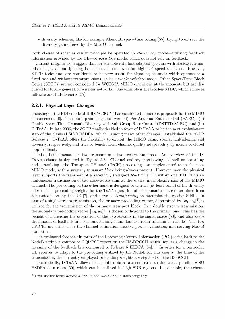
Chapter 2. HSDPA and its MIMO Enhancements
• diversity schemes, like for example Alamouti space-time coding [55], trying to extract thediversity gain offered by the MIMO channel.
Both classes of schemes can in principle be operated in closed loop mode—utilizing feedbackinformation provided by the UE—or open loop mode, which does not rely on feedback.
Current insights [56] suggest that for variable rate link adapted systems with HARQ retrans-mission spatial multiplexing is the best choice, even for high UE speed scenarios. However,STTD techniques are considered to be very useful for signaling channels which operate at afixed rate and without retransmissions, called un-acknowledged mode. Other Space-Time BlockCodes (STBCs) are not considered for WCDMA MIMO extensions at the moment, but are dis-cussed for future generation wireless networks. One example is the Golden-STBC, which achievesfull-rate and full-diversity [57].
2.2.1. Physical Layer Changes
Focusing on the FDD mode of HSDPA, 3GPP has considered numerous proposals for the MIMOenhancement [6]. The most promising ones were (i) Per-Antenna Rate Control (PARC), (ii)Double Space-Time Transmit Diversity with Sub-Group Rate Control (DSTTD-SGRC), and (iii)D-TxAA. In late 2006, the 3GPP finally decided in favor of D-TxAA to be the next evolutionarystep of the classical SISO HSDPA, which—among many other changes—established the 3GPPRelease 7. D-TxAA offers the flexibility to exploit the MIMO gains, spatial multiplexing anddiversity, respectively, and tries to benefit from channel quality adaptability by means of closedloop feedback.
This scheme focuses on two transmit and two receive antennas. An overview of the D-TxAA scheme is depicted in Figure 2.8. Channel coding, interleaving, as well as spreadingand scrambling—the Transport CHannel (TrCH) processing—are implemented as in the non-MIMO mode, with a primary transport block being always present. However, now the physicallayer supports the transport of a secondary transport block to a UE within one TTI. This si-multaneous transmission of two code-words aims at the spatial multiplexing gain of the MIMOchannel. The pre-coding on the other hand is designed to extract (at least some) of the diversityoffered. The pre-coding weights for the TxAA operation of the transmitter are determined froma quantized set by the UE [7], and serve as beamforming to maximize the receive SINR. Incase of a single-stream transmission, the primary pre-coding vector, determined by [w1, w2]T, isutilized for the transmission of the primary transport block. In a double stream transmission,the secondary pre-coding vector [w3, w4]T is chosen orthogonal to the primary one. This has thebenefit of increasing the separation of the two streams in the signal space [58], and also keepsthe amount of feedback bits constant for single and double stream transmission modes. The twoCPICHs are utilized for the channel estimation, receive power evaluation, and serving NodeBevaluation.
The evaluated feedback in form of the Precoding Control Information (PCI) is fed back to theNodeB within a composite CQI/PCI report on the HS-DPCCH which implies a change in themeaning of the feedback bits compared to Release 5 HSDPA [34].13 In order for a particularUE receiver to adapt to the pre-coding utilized by the NodeB for this user at the time of thetransmission, the currently employed pre-coding weights are signaled on the HS-SCCH.
Theoretically, D-TxAA allows for a doubled data rate compared to the actual possible SISOHSDPA data rates [59], which can be utilized in high SNR regions. In principle, the scheme13I will use the terms Release 5 HSDPA and SISO HSDPA interchangeably.
20
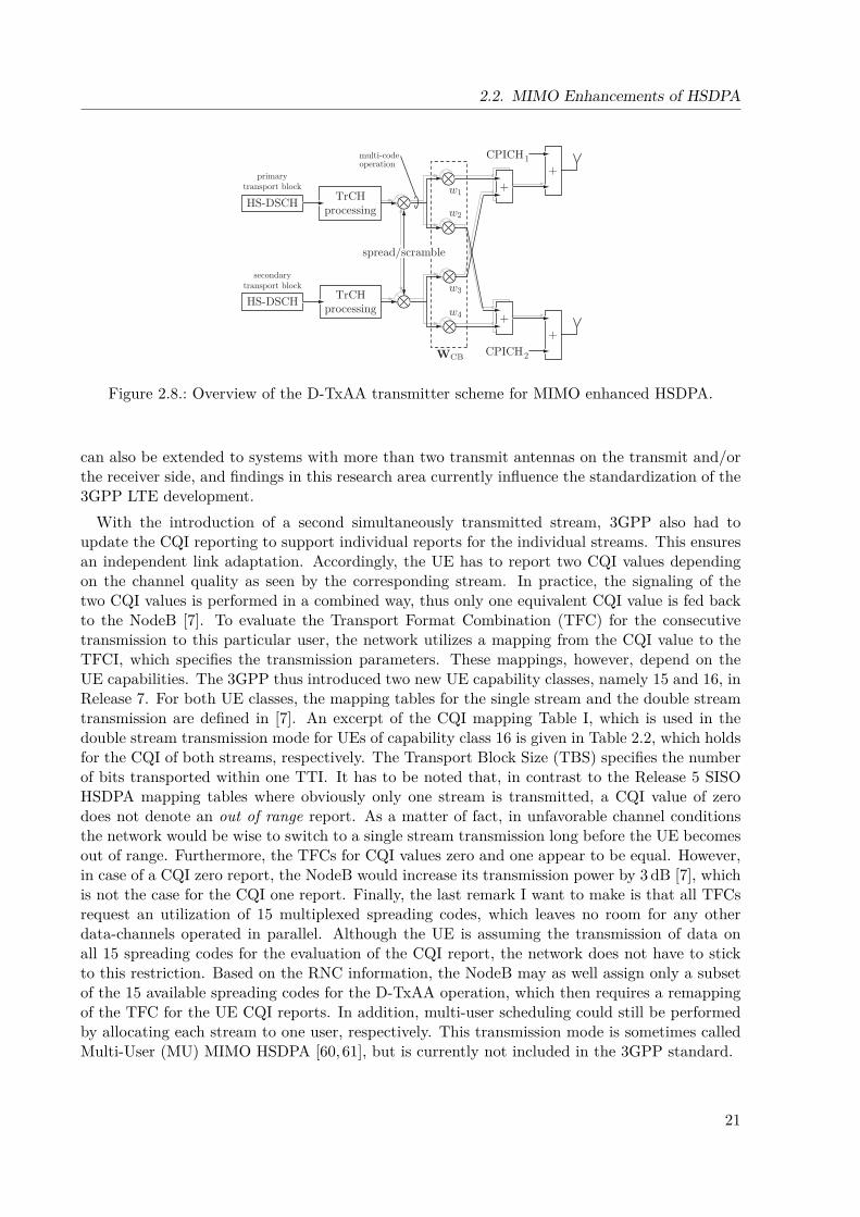
2.2. MIMO Enhancements of HSDPA
HS-DSCH TrCHprocessing
++
HS-DSCH TrCHprocessing
++
CPICH1
CPICH2
primarytransport block
secondarytransport block
spread/scramble
multi-codeoperation
Figure 2.8.: Overview of the D-TxAA transmitter scheme for MIMO enhanced HSDPA.
can also be extended to systems with more than two transmit antennas on the transmit and/orthe receiver side, and findings in this research area currently influence the standardization of the3GPP LTE development.
With the introduction of a second simultaneously transmitted stream, 3GPP also had toupdate the CQI reporting to support individual reports for the individual streams. This ensuresan independent link adaptation. Accordingly, the UE has to report two CQI values dependingon the channel quality as seen by the corresponding stream. In practice, the signaling of thetwo CQI values is performed in a combined way, thus only one equivalent CQI value is fed backto the NodeB [7]. To evaluate the Transport Format Combination (TFC) for the consecutivetransmission to this particular user, the network utilizes a mapping from the CQI value to theTFCI, which specifies the transmission parameters. These mappings, however, depend on theUE capabilities. The 3GPP thus introduced two new UE capability classes, namely 15 and 16, inRelease 7. For both UE classes, the mapping tables for the single stream and the double streamtransmission are defined in [7]. An excerpt of the CQI mapping Table I, which is used in thedouble stream transmission mode for UEs of capability class 16 is given in Table 2.2, which holdsfor the CQI of both streams, respectively. The Transport Block Size (TBS) specifies the numberof bits transported within one TTI. It has to be noted that, in contrast to the Release 5 SISOHSDPA mapping tables where obviously only one stream is transmitted, a CQI value of zerodoes not denote an out of range report. As a matter of fact, in unfavorable channel conditionsthe network would be wise to switch to a single stream transmission long before the UE becomesout of range. Furthermore, the TFCs for CQI values zero and one appear to be equal. However,in case of a CQI zero report, the NodeB would increase its transmission power by 3 dB [7], whichis not the case for the CQI one report. Finally, the last remark I want to make is that all TFCsrequest an utilization of 15 multiplexed spreading codes, which leaves no room for any otherdata-channels operated in parallel. Although the UE is assuming the transmission of data onall 15 spreading codes for the evaluation of the CQI report, the network does not have to stickto this restriction. Based on the RNC information, the NodeB may as well assign only a subsetof the 15 available spreading codes for the D-TxAA operation, which then requires a remappingof the TFC for the UE CQI reports. In addition, multi-user scheduling could still be performedby allocating each stream to one user, respectively. This transmission mode is sometimes calledMulti-User (MU) MIMO HSDPA [60,61], but is currently not included in the 3GPP standard.
21
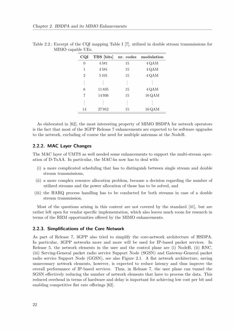
Chapter 2. HSDPA and its MIMO Enhancements
Table 2.2.: Excerpt of the CQI mapping Table I [7], utilized in double stream transmissions forMIMO capable UEs.
CQI TBS [bits] nr. codes modulation0 4 581 15 4 QAM1 4 581 15 4 QAM2 5 101 15 4 QAM...
......
...6 11 835 15 4 QAM7 14 936 15 16 QAM...
......
...14 27 952 15 16 QAM
As elaborated in [62], the most interesting property of MIMO HSDPA for network operatorsis the fact that most of the 3GPP Release 7 enhancements are expected to be software upgradesto the network, excluding of course the need for multiple antennas at the NodeB.
2.2.2. MAC Layer ChangesThe MAC layer of UMTS as well needed some enhancements to support the multi-stream oper-ation of D-TxAA. In particular, the MAC-hs now has to deal with:
(i) a more complicated scheduling that has to distinguish between single stream and doublestream transmissions,
(ii) a more complex resource allocation problem, because a decision regarding the number ofutilized streams and the power allocation of those has to be solved, and
(iii) the HARQ process handling has to be conducted for both streams in case of a doublestream transmission.
Most of the questions arising in this context are not covered by the standard [41], but arerather left open for vendor specific implementation, which also leaves much room for research interms of the RRM opportunities offered by the MIMO enhancements.
2.2.3. Simplifications of the Core NetworkAs part of Release 7, 3GPP also tried to simplify the core-network architecture of HSDPA.In particular, 3GPP networks more and more will be used for IP-based packet services. InRelease 5, the network elements in the user and the control plane are (i) NodeB, (ii) RNC,(iii) Serving-General packet radio service Support Node (SGSN) and Gateway-General packetradio service Support Node (GGSN), see also Figure 2.1. A flat network architecture, savingunnecessary network elements, however, is expected to reduce latency and thus improve theoverall performance of IP-based services. Thus, in Release 7, the user plane can tunnel theSGSN effectively reducing the number of network elements that have to process the data. Thisreduced overhead in terms of hardware and delay is important for achieving low cost per bit andenabling competitive flat rate offerings [62].
22
Chapter 3.
System-Level Modeling of MIMO-EnhancedHSDPA
While all models are unrealistic,some of them are actually useful.
(George Box)
Useful modeling in the context of wireless networks is in general a difficult task, whichrequires careful investigations of many different parameter settings and a design that avoids
leading to potentially wrong conclusions. System-level modeling is particularly demanding inthis sense, because in addition to the design requirements, the computational complexity playsa crucial role.
So what is system-level modeling all about? One thing that emerges when investigating theterm system-level is that it is quite extensively1 used in the literature. As a matter of fact,every comprehensive investigation of a technical system—not only in the context of a cellularsystem—may be denoted system-level analysis. Examples are electronic design methodology,virtualization for operating systems, hardware-software co-design for Very High Speed IntegratedCircuits (VHSIC), or network synthesis. In the scope of this work however, the term system-levelmodel describes:
A model capable of representing the physical layer of a wireless transmission systemin an abstract, yet accurate way that is less complex to evaluate than computing allthe algorithms and reproducing all relevant effects involved in the physical layer intheir full detail, and can be described by a low number of parameters.
Given this rather conceptional definition, what are system-level models needed for? Usually,physical-layer simulations are used to identify and evaluate promising transmission techniques.Whereas these investigations are suitable for the deployment of receiver algorithms, feedbackstrategies, coding design, and so on, they are not directly capable of reflecting network issueslike cell planing, scheduling, and interference situations in the context of massive multi-useroperation [14]. Therefore, to understand the network and user performance under typical oper-ating conditions in various deployment scenarios, network simulations are crucial [63–65]. Sucha wireless network defines the system to which the term system-level is referring. Accordingly,system-level simulations are built to comprise the full network, thus trying to cover at least
(i) network deployment issues including network performance [26,66,67],(ii) multi-user and multi-NodeB (inter-cell) interference [68–70],(iii) RLC and admission control algorithms [71,72], as well as1For example, a search for the term system level on Google returned approximately 3 160 000 hits.
23

Chapter 3. System-Level Modeling of MIMO-Enhanced HSDPA
(iv) scheduling [73,74].
One of the major difficulties of system-level analyses, however, is the computational complexityinvolved in evaluating the performance of the radio links between all base-stations and mobileterminals. Performing such a large number of individual physical-layer—or also often calledlink-level—simulations is clearly prohibitive in terms of the computational complexity. Thus, asystem-level model has to simplify the physical link in a sufficiently accurate way to capture theessential behavior [12,75–78].
To summarize, an ideal system-level model has to be (i) sufficiently accurate, (ii) flexible interms of the scenarios it is capable of representing, as well as applicable for analytic investigations,(iii) implementable with very low computational complexity, and (iv) describable by a reasonablenumber of parameters. However, even an ideal model can have some traps. Let me put someadvisable mistrust in the words of [79].
• Don’t believe in the 33rd order consequences of a 1st order model. Catch phrase: Cumgrano salis.2
• Don’t extrapolate beyond the region of fit. Catch phrase: Don’t go off the deep end.• Don’t believe the model is reality. Catch phrase: Don’t eat the menu.• Don’t fall in love with your model. Catch phrase: Pygmalion.3
3.1. Concept of System-Level ModelingAfter having defined the scope of a system-level model, it remains to sketch the concept behind it.As already mentioned, the basic idea is to find a suitable mathematical abstraction of the physicallayer. Generally speaking, such a model consists of two concatenated parts. To illustrate that,Figure 3.1 shows a very abstract view of the transmission in a wireless communication system.Here, the whole transmission chain is divided in a first part handling the physical layer processing,which includes in HSDPA
• spreading/de-spreading, scrambling/de-scrambling• modulation,• pre-coding, space-time coding,• channel estimation, synchronization, and• receiver processing,
and a second part handling the channel encoding and decoding including in HSDPA
• turbo coding/decoding,• interleaving, rate-matching, HARQ, and• demapping.
2The direct translation would be: With a grain of salt, however, the saying is nowadays used to advise the readerthat the point made should not be taken literally in every aspect.
3According to Ovid, Pygmalion is a legendary figure of Cyprus. He is told to have been a sculptor who falls inlove with a statue he has made.
24

3.1. Concept of System-Level Modeling
source sink
chan
nel
enco
ding
chan
nel
deco
ding
physical-layerprocessing
transmitter receiver
physical-layer quality
transmission performance
multi-user system-level representation
Figure 3.1.: Abstract illustration of the transmission chain in wireless communication systems.
Note that both parts incorporate the transmitter and the receiver, respectively. When intro-ducing a split like that, the physical-layer processing can be modeled by a link-quality model,4which describes the physical-layer quality, and a link-performance model, describing the transmis-sion performance with respect to the channel coding and decoding. For system-level purposes,the link-quality model has to incorporate the effects of
• the interference structure, that is intra-cell and inter-cell interference, incorporating possi-ble multi-user interference (see again Figure 3.1),• the influence of other channels than the evaluated one, for example the synchronization
channel, or other DCH channels,• the power allocation in the cell as well as in the whole network, and• the channel effects, in particular the macro-scale pathloss, the antenna gain, the shadow-
fading and the small-scale fading.
At this point it is important to note that the small-scale5 fading has to be covered by the system-level model to allow for the accurate evaluation of NodeB-based schedulers, which operate on a2 ms TTI basis in HSDPA. If those effects are covered, such a system-level model is often referredto as actual value interface [81, 83].
The link-performance model then has to—based on the evaluations of the link-quality model—represent the coding/decoding performance in terms of the BLER, given a link-adaptation strat-egy [84]. Considering the flexibility of the HSDPA physical layer, this model has to cover a widerange of conditions. Together, both models provide means to assess the figures of merit in asystem-level context, and they are often commonly referred to as system-level interface.
Figure 3.2 depicts the relations of the two models in a system-level approach. On top of thealready mentioned influencing factors, the figure also shows the connection to the algorithms anddeployment issues that influence the system performance. In particular,
4This model is also often called link-measurement model [80]. However, in this work I will stick to the moredescriptive term link-quality model.
5Sometimes in the system-level literature, for example [64, 81], the small-scale fading is denoted fast fading, inorder to point out the difference to slowly changing channel effects like shadow-fading. However, the notationfast strongly depends on the relative speed of the transmitter, the receiver, and the channel, thus renderingthis term rather inaccurate. Furthermore, the classical literature [82], defines fast fading to be fading whichchanges the channel condition within the duration of one symbol, which is usually not modeled in the system-level context. Accordingly, in the context of this work I will stick to the term small-scale fading for Rayleighfading like effects.
25
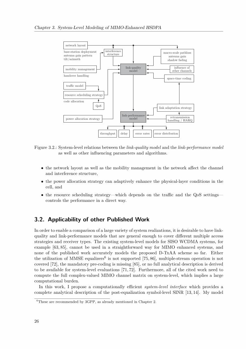
Chapter 3. System-Level Modeling of MIMO-Enhanced HSDPA
link-performancemodel
link-qualitymodel
space-time coding
influence ofother channels
interferencestructure macro-scale pathloss
antenna gainshadow fading
throughput delay error rates error distribution
traffic model
link adaptation strategy
resource scheduling strategy
QoScode allocation
power allocation strategy
network layout
base-station deploymentantenna gain patterntilt/azimuth
mobility management
handover handling
retransmissionhandling / HARQ
Figure 3.2.: System-level relations between the link-quality model and the link-performance modelas well as other influencing parameters and algorithms.
• the network layout as well as the mobility management in the network affect the channeland interference structure,
• the power allocation strategy can adaptively enhance the physical-layer conditions in thecell, and
• the resource scheduling strategy—which depends on the traffic and the QoS settings—controls the performance in a direct way.
3.2. Applicability of other Published Work
In order to enable a comparison of a large variety of system realizations, it is desirable to have link-quality and link-performance models that are general enough to cover different multiple accessstrategies and receiver types. The existing system-level models for SISO WCDMA systems, forexample [63, 85], cannot be used in a straightforward way for MIMO enhanced systems, andnone of the published work accurately models the proposed D-TxAA scheme so far. Eitherthe utilization of MMSE equalizers6 is not supported [75, 86], multiple-stream operation is notcovered [72], the mandatory pre-coding is missing [85], or no full analytical description is derivedto be available for system-level evaluations [71, 72]. Furthermore, all of the cited work need tocompute the full complex-valued MIMO channel matrix on system-level, which implies a largecomputational burden.
In this work, I propose a computationally efficient system-level interface which provides acomplete analytical description of the post-equalization symbol-level SINR [13, 14]. My model
6These are recommended by 3GPP, as already mentioned in Chapter 2.
26
3.3. Computationally Efficient Link-Quality Model
shows a structure that identifies the relevant interference terms which enables for example alsoreceiver optimizations [22,23]. Parts of the contents of this chapter have been published in [12–14,16,17,26].
One of the crucial components of the model is that it allows for the generation of so-calledfading parameters, prior to the system-level simulation itself. These fading parameters includenearly all link-related procedures, thus during the runtime of the system-level simulation onlyscalar real-valued multiplications are needed to compute the SINR. This significantly reducesthe computational effort. In principle, this idea has already been touched in [78] for WCDMAUMTS, however in the context of MIMO it has to be generalized and fairly extended to beutilizable to derive a suitable description.
3.3. Computationally Efficient Link-Quality ModelTo be able to derive an accurate and computationally efficient system-level model, an analyticalmodel of the MIMO HSDPA link quality is needed. The basics of the physical layer transmissionhave already been defined in Chapter 2. In particular the D-TxAA mode [6] is depicted inFigure 2.8. To represent this transmission setting, I adapted the framework of [87] in order toreflect one individual link between a NodeB and a UE.
Figure 3.3 depicts the model where the transmitter and the receiver are equipped with NT andNR antennas, respectively. Note that this description allows for the modeling of more than twospatial multiplexed data streams, which is the maximum supported by Release 7 MIMO HSDPA.Accordingly, as illustrated in Figure 3.3, NS parallel data streams s(0), . . . , s(NS−1) enter the sys-tem. Each data stream s(n), n = 1, . . . , NS is individually encoded and modulated, like depictedin Figure 2.8, and is then being spread by a number of spreading sequences ϕ(n)
k with k specify-ing the individual spreading code. This represents multi-code usage on each stream. The set ofindividual spreading codes utilized for stream n is denoted Φn, thus ϕ(n)
k ∈ Φn. The streams areof course scrambled as well, but for sake of clarity, I did not depict the scrambling/descrambling.Let me, however, still denote the scrambling sequence utilized for this particular link by ψ.Assumption 3.1. There is only one scrambling code active for each link.
Thus both streams are scrambled with the same scrambling sequence,7 however the NodeBcould still apply different scrambling codes for different users. Note that by this convention, themodel does not allow individual streams to be separately scrambled. The inverse operations ofthe spreading and scrambling at the receiver side are consequently denoted ϕ
(n)k and ψ.
The spread and scrambled sequences x(n), n = 1, . . . , NS are then mapped to the NT transmitantennas using the pre-coding matrix WCB ∈ CNT×NS , which contains the pre-coding weightsw1, . . . , wNTNS , similar to Figure 2.8, where WCB is defined by w1, . . . , w4. At the receiver, thesignals are gathered with NR antennas and chip spaced sampled before they enter the discrete-time receive filter. The MIMO channel H ∈ CNR×NTLh is modeled as time-discrete, frequency-selective channel,
H =
h
(1,1)0 · · · h
(1,NT)0 h
(1,1)1 · · · h
(1,NT)1 · · · h
(1,NT)Lh−1 · · · h
(1,NT)Lh−1
......
...... . . . ...
...h
(NR,1)0 · · · h
(NR,NT)0 h
(NR,1)1 · · · h
(NR,NT)1 · · · h
(NR,NT)Lh−1 · · · h
(NR,NT)Lh−1
. (3.1)
7The scrambling code is, as opposed to the spreading code, is not targeted for a spreading of the utilizedbandwidth, but rather to separate cells in the downlink and users in the uplink. The scrambling codes aredesigned specifically to show good cross-correlation properties (Gold codes).
27

Chapter 3. System-Level Modeling of MIMO-Enhanced HSDPA
rece
ive
filte
r
spreading,scrambling
frequency selectiveMIMO channel
descrambling,despreading
Figure 3.3.: System model for a WCDMA system, reflecting the parallel transmission of NSstreams over NT transmit antennas and reception with NR receive antennas utilizinga receive filter.
The entry h(nr,nt)l , l = 0, . . . , Lh−1, nr = 1, . . . , NR, nt = 1, . . . , NT denotes the l-th sampled chip
of the channel impulse response from transmit antenna nt to receive antenna nr, with a totalchannel length of Lh chip intervals. Note that pulse-shaping, transmit and receive band-filtering,as well as the sampling operation can be incorporated in the MIMO channel matrix. To accountfor the pre-coding, I define an equivalent time-discrete channel Hw ∈ CNR×NSLh that includesthe pre-coding matrix WCB and the MIMO channel,
Hw , H (ILh ⊗WCB) , (3.2)
with ILh denoting the identity matrix of size Lh × Lh, and ⊗ being the Kronecker product.Furthermore, let me define the transmit and receive vectors as
yi ,[y
(1)i · · · y
(NR)i
]T, (3.3)
xi ,[x
(0)i · · · x
(NS−1)i x
(0)i−1 · · · x
(NS−1)i−1 · · · x
(0)i−Lh+1 · · · x
(NS−1)i−Lh+1
]T, (3.4)
and the noise vector as
ni ,[n
(1)i · · · n
(NR)i
]T, (3.5)
with i ∈ N denoting the discrete-time index, like in Chapter 2. Then the input-output relationfor one link, formulated by means of the equivalent MIMO channel matrix, is given by
yi = Hwxi + ni. (3.6)
The description in Equation (3.6) certainly allows for the description of the D-TxAA schemewhich implies that NT = NR = 2 and NS = 1, 2. However, the input-output relation can be usedfor more than two independent data streams, thus supporting possible future extensions of thescheme, or other transmission schemes like [15].
3.3.1. EqualizerTo derive a suitable link-quality model also the receive filter has to be taken into account.Assumption 3.2. Only linear equalizers at the receiver are considered.
28
3.3. Computationally Efficient Link-Quality Model
This accordingly excludes Successive Interference Cancellation (SIC) receivers as well as MLbased structures. Note that currently Release 5 HSDPA devices utilize a Rake-receiver [88], andRelease 7 HSDPA devices are recommended to employ MMSE equalizers [89]. Thus, this restric-tion does not impose a dramatic problem for current networks, however, for further enhancedset-ups, the modeling would have to be refined at this point.
For the derivation of the receive filter, the input-ouput relation in Equation (3.6) has to beextended for Lf received chips at the NR receive antennas, specifying the filter length. By definingthe stacked versions of the parameters introduced so far,
yi ,[yTi . . . yT
i−Lf+1
]T, (3.7)
xi ,[x
(0)i · · · x
(NS−1)i x
(0)i−1 · · · x
(NS−1)i−1 · · · x
(0)i−Lh−Lf+2 · · · x
(NS−1)i−Lh−Lf+2
]T, (3.8)
and
ni ,[nTi · · · nT
i−Lf+1
]T, (3.9)
as well as the stacked equivalent MIMO channel matrix Hw ∈ CNRLf×NS(Lh+Lf−1),
Hw ,
Hw 0NR,NS · · · 0NR,NS
0NR,NS Hw 0NR,NS... . . .
0NR,NS 0NR,NS · · · Hw
, (3.10)
where 0NR,NS denotes the all-zero matrix of dimension NR × NS, the input-output relation be-comes
yi = Hwxi + ni. (3.11)
Note, however, that the stacked equivalent channel matrix Hw cannot be represented by a Kro-necker product, because the matrix does not have a block diagonal structure, as indicated by thesize of the matrices 0NR,NS .
One particular example of a receive filter that—as already mentioned is recommended bythe 3GPP for Release 7 HSDPA—is the MMSE equalizer. For the input output relation ofEquation (3.11), the cost function of the MMSE receiver can be formulated as
J(F) = E∥∥∥Fyi − xS
i−τ
∥∥∥2, (3.12)
where τ defines the delay of the MMSE filter, which has to fulfill τ ≥ Lh to include at least allobservations affected by xi. The vector of transmit chips to be estimated is defined as
xSi−τ ,
[x
(0)i−τ · · · x
(NS−1)i−τ
]T, (3.13)
thus representing the chips of all transmitted streams at time index i − τ . A filter satisfyingEquation (3.12) tries to restore the orthogonality of the individual spreading codes caused bythe multi-path propagation. This problem has already been investigated, for example in [87,90],and its solution turns out to be given by the suitable formulated Wiener-Hopf equation, leadingto
F = RxSi−τ xiH
Hw
(HwRxiHH
w + Rni
)−1. (3.14)
29
Chapter 3. System-Level Modeling of MIMO-Enhanced HSDPA
Assuming white, i.i.d., uncorrelated transmit sequences, the covariance matrices can be evaluatedto have the following structure,
RxSi−τ xi =
[0NS×NSτ P 0NS×NS(Lf+Lh−τ+2)
], (3.15)
Rxi = ILf+Lh−1 ⊗P, (3.16)
with
P , diag[P1 · · · Pn · · · PNS
](3.17)
specifying the powers utilized on each stream n, Pn = E∣∣∣x(n)
i
∣∣∣2 = σ2x
(n)i
, respectively.The equalizer length Lf and the detection delay τ are important parameters that influence the
performance of the system, but an optimization of these is not within the scope of this work.Assumption 3.3. The equalizer delay is set to τ = Lf/2, see for example [89].
Note that this choice does not affect the system-level modeling itself, but the simulation resultspresented in Section 3.3.4.
3.3.2. WCDMA MIMO in the Network Context
In a multi-cell, multi-user scenario, Equation (3.11) has to be extended to cover the signals fromall sectors and all users, as well as all spreading codes that are active at that moment. Todo so, let me define the transmit—and accordingly the receive sequence—in Equation (3.11) tocorrespond to a set of utilized spreading and scrambling sequences,
xi =∑ϕk∈Φ
x(ϕk,ψ)i , (3.18)
where ϕk ∈ Φ,Φ , Φ0 ∪ · · · ∪ ΦNS−1. The entries of x(ϕk,ψ)i additionally have to fulfill
x(n),(ϕk,ψ)i ,
x(n)i : ϕ(n)
k = ϕk,
0 : ϕ(n)k 6= ϕk,
(3.19)
which allows for representing cases in which different streams utilize only partly-, or even non-overlapping spreading code sets Φn, n = 0, . . . , NS − 1.
Furthermore, let me index the users of a sector by the pair (u, b) with u = 1, . . . , U(b), becausethe number of active users can be different for each sector b, and b = 1, . . . , B. I used theterm sector here, because potentially every sector of a NodeB can be independently controlledin terms of its radio resources, that is, the power and spreading code allocation. In principle,a link in a sectored network would be specified by the triple user, sector, base-station, (u, z, b),where z = 1, . . . , Z(b) and b denote the sector and base-station index, respectively. For sake ofnotational simplicity, however, I chose to index the sectors individually, for which I used b as theindex. In most practical networks, the number of sectors per base-station is constant, thus notimposing the need to identify the links by the triple. For a single-sector network, the pair (u, b)is obviously sufficient as well. Thus, the transmit signal of one particular link utilizing a givenspreading and scrambling code pair is denoted x(ϕk,ψ),(u,b)
i .
30
3.3. Computationally Efficient Link-Quality Model
With the individual link being specified by (u, b), the set of utilized spreading codes on thatlink is denoted by Φ(u,b). This, however, would require the pair of spreading and scramblingsequences to be indexed by (u, b), that is, ϕk → ϕ
(u,b)k and ψ → ψ(u,b) to be mathematically
precise. Nevertheless I dropped these indices, again for sake of notational simplicity. By thesedefinitions, the power of one stream n on link (u, b), is given by
P (u,b)n = E
∣∣∣∣∣∣∣
∑ϕ
(n)k∈Φ(u,b)
n
x(n),(ϕ(n)
k,ψ),(u,b)
i
∣∣∣∣∣∣∣2 =
∑ϕ
(n)k∈Φ(u,b)
n
σ2
x(n),(ϕ(n)
k,ψ),(u,b)
i
=∑
ϕ(n)k∈Φ(u,b)
n
P(u,b)n,ϕ
(n)k
,
(3.20)with P
(u,b)n,ϕ
(n)k
denoting the power on stream n and spreading code ϕ(n)k for the link (u, b).
Assumption 3.4. For Equation (3.20) to hold, the data sequences on the individual spreadingcodes are uncorrelated.
The interference on one particular user u0, which I will call the desired user, is received overB frequency selective MIMO channels. This is the user for whom the physical-layer quality hasto be evaluated. The base-station/sector to which this user is attached to with index b0 will becalled target sector in the following. However, due to the user specific pre-coding, the equivalentchannel matrix Hw will be different for different individual users. Accordingly, let me index thechannel matrices involved in the network context as H(u,b)
w . Using these definitions, the totalreceived signal at the desired user can be evaluated by summation over all active sectors andusers, as well as spreading codes, respectively,
y(u0)i =
B∑b=1
U(b)∑u=1
∑ϕk∈Φ(u,b)
H(u,b)w x(ϕk,ψ),(u,b)
i + ni. (3.21)
The received signal is then passed through the receive filter, which leads to the useful post-equalization signal given by
x(u0)i =
B∑b=1
U(b)∑u=1
∑ϕk∈Φ(u,b)
FH(u,b)w x(ϕk,ψ),(u,b)
i + Fni. (3.22)
To analyze this relation and identify the different interference terms, it is necessary to decomposethe receive filter into the according filters responsible for each stream,
F =[f (0) · · · f (n) · · · f (NS−1)
]T, (3.23)
as well as the channel matrix into its columns,
H(u,b)w =
[h(u,b)
0 · · · h(u,b)m · · · h(u,b)
NS(Lf+Lh−1)−1
], (3.24)
where m is the index of the transmit chips for all streams entering the receive filter. Accordingly,the post-equalization signal of Equation (3.22) for stream n can be written as
x(n),(u0)i =
B∑b=1
U(b)∑u=1
∑ϕk∈Φ(u,b)
NS(Lf+Lh−1)−1∑m=0
(f (n)
)Th(u,b)m x
(bm/NSe),(ϕk,ψ),(u,b)i−bm/NSc +
(f (n)
)Tni, (3.25)
31
Chapter 3. System-Level Modeling of MIMO-Enhanced HSDPA
where bm/NSe denotes the remainder of the integer division which represents the index of thesubstream, and bm/NSc denotes the largest integer smaller than m/NS which corresponds to thedelay of the transmit chip.
After the receive filtering x(n),(u0)i is multiplied with the complex conjugated scrambling and
spreading codes and integrated over the period of a symbol8 to obtain the estimated transmitsymbols s(n) for stream n, respectively.
3.3.3. Description of the Equivalent Fading Parameters
Nearly all relevant performance metrics in wireless communications are evaluated with respect toSINR. Accordingly, I am deriving a suitable description of the SINR as observed in the networkcontext to represent the physical-layer quality. The applicability of the SINR in order to predictthe BLER performance of the overall transmission scheme also seems intuitive.
Assumption 3.5. In the following, the NodeB utilizes only one scrambling sequence for all of itslinks.
Also note that this reflects a typical WCDMA scenario as currently implemented for Release 5HSDPA and simplifies the notation, thus in the following I will not use the index ψ anymore.For the derivation of the SINR, Equation (3.25) has to be decomposed into the different relevantinterference and desired signal power terms. Note that all of the following power terms apply tothe desired user u0 and target sector b0.
Desired Signal
The power of the desired signal on stream n and spreading code ϕk is given by the resultingpower after the receive filter at delay τ ,
P sn,ϕk
, P s,(u0,b0)n,ϕk
=∣∣∣∣(f (n)
)Th(u0,b0)τNS+n
∣∣∣∣2 P (u0,b0)n,ϕ
(n)k
, (3.26)
where I dropped the indication of the desired user and sector in the resulting power term for sakeof notational simplicity. The idea now is to define the desired signal power as the multiplicationof the power on stream n and spreading code ϕ(n)
k —which is known in a system-level simulation—with a so-called equivalent fading parameter. Here, the equivalent fading parameter of the desiredsignal on stream n, Gs
n, also called desired signal gain, is defined as
Gsn ,
∣∣∣∣(f (n))T
h(u0,b0)τNS+n
∣∣∣∣2 ⇒ P sn,ϕk
= GsnP
(u0,b0)n,ϕ
(n)k
. (3.27)
This fading parameter contains the full information about the consequences of the physical-layeronto the desired signal.
Intra-cell Interference
The intra-cell interference is composed by a number of terms, in particular8Which corresponds to SF chip periods Tc, with Tc = 1/3840000 s in WCDMA systems.
32
3.3. Computationally Efficient Link-Quality Model
• the remaining Inter-Symbol Interference (ISI) after equalization,
P ISIn,ϕk
, P ISI,(u0,b0)n,ϕk
=NS(Lf+Lh−1)−1∑
m=0m 6∈[τNS,τNS+NS−1]
∣∣∣∣(f (n))T
h(u0,b0)m
∣∣∣∣2 P (u0,b0)bm/NSe,ϕ
(bm/NSe)k
, (3.28)
• the inter-code interference when the same scrambling but a different spreading code is used,
P ICn,ϕk
, P IC,(u0,b0)n,ϕk
=NS(Lf+Lh−1)−1∑
m=0m 6∈[τNS,τNS+NS−1]
∣∣∣∣(f (n))T
h(u0,b0)m
∣∣∣∣2 ∑ϕk∈Φ(u,b)
ϕk 6=ϕk
P(u0,b0)bm/NSe,ϕ
(bm/NSe)k
, (3.29)
• the time-aligned intra-cell interference from users with the same spreading code as thedesired user,
P intra1n,ϕk
, P intra1,(u0,b0)n,ϕk
=U(b0)∑u=1u6=u0
τNS+NS−1∑m=τNS
∣∣∣∣(f (n))T
h(u,b0)m
∣∣∣∣2 P (u,b0)bm/NSe,ϕ
(bm/NSe)k
, (3.30)
• the not time-aligned intra-cell interference from users with the same spreading code causedby multi-path propagation,
P intra2n,ϕk
, P intra2,(u0,b0)n,ϕk
=U(b0)∑u=1u6=u0
NS(Lf+Lh−1)−1∑m=0
m 6∈[τNS,τNS+NS−1]
∣∣∣∣(f (n))T
h(u,b0)m
∣∣∣∣2 P (u,b0)bm/NSe,ϕ
(bm/NSe)k
, (3.31)
• and the intra-cell interference from users with the same scrambling code, but differentspreading code
P intra3n,ϕk
, P intra3,(u0,b0)n,ϕk
=U(b0)∑u=1u6=u0
NS(Lf+Lh−1)−1∑m=0
m6∈[τNS,τNS+NS−1]
∣∣∣∣(f (n))T
h(u,b0)m
∣∣∣∣2 ∑ϕk∈Φ(u,b)
ϕk 6=ϕk
P(u,b0)bm/NSe,ϕ
(bm/NSe)k
. (3.32)
As already mentioned, due to the assumption that there is only one scrambling code per link, aswell as the more restrictive assumption that the NodeB uses only one scrambling code overall, nointerference term for inter-scrambling code interference appears in the context of the intra-cellinterference. Furthermore, let me point out that in a practical system implementation of MIMOHSDPA, it is not very likely that other users will be scheduled in parallel to the desired userutilizing the same—or even overlapping—spreading code sets. In such a case, the users wouldonly be separated by means of SDMA, and the resulting interference is increased by the spreadinggain.
Assumption 3.6. Accordingly, no pure SDMA user separation is performed, which implies that
P intra1n,ϕk
= 0. (3.33)
33

Chapter 3. System-Level Modeling of MIMO-Enhanced HSDPA
From the remaining terms P ISIn,ϕk
and P ICn,ϕk
represent the intra-cell interference generated bythe desired user himself, which can be called self interference,
P selfn,ϕk
, P ISIn,ϕk
+ P ICn,ϕk
=NS(Lf+Lh−1)−1∑
m=0m6∈[τNS,τNS+NS−1]
∣∣∣∣(f (n))T
h(u0,b0)m
∣∣∣∣2 P (u0,b0)bm/NSe. (3.34)
Similarly, P intra2n,ϕk
and P intra3n,ϕk
specify the intra-cell interference generated by all other users in thesector, which may be called other-user interference,
P othern,ϕk
, P intra2n,ϕk
+ P intra3n,ϕk
=U(b0)∑u=1u6=u0
NS(Lf+Lh−1)−1∑m=0
m6∈[τNS,τNS+NS−1]
∣∣∣∣(f (n))T
h(u,b0)m
∣∣∣∣2 P (u,b0)bm/NSe. (3.35)
Assumption 3.7. For the overall intra-cell interference, all streams n = 0, . . . , NS− 1 transmittedto a user u have the same power,
P (u,b)n ≡ 1
NSP (u,b), (3.36)
with P (u,b) denoting the total power spent for user u by sector b.
Note that this limits the applicability of the model to cases where no dynamic power loadingfor the individual streams takes place. For more advanced power resource allocation, for examplewater-filling idea based algorithms, the model would have to be refined at this point.
Consequently, the total intra-cell interference, as seen by the desired user u0 on stream n andspreading code ϕk, becomes
P intran,ϕk
= P selfn,ϕk
+ P othern,ϕk
= 1NS
P (u0,b0)NS(Lf+Lh−1)−1∑
m=0m 6∈[τNS,τNS+NS−1]
∣∣∣∣(f (n))T
h(u0,b0)m
∣∣∣∣2︸ ︷︷ ︸
self interference
+ 1NS
U(b0)∑u=1u6=u0
P (u,b0)NS(Lf+Lh−1)−1∑
m=0m6∈[τNS,τNS+NS−1]
∣∣∣∣(f (n))T
h(u,b0)m
∣∣∣∣2︸ ︷︷ ︸
other-user interference
.
(3.37)
So far, Equation (3.37) still does not allow for a decoupling into equivalent fading parametersand power terms, because h(u,b0)
m depends on the user index, and in particular on the choice ofthe users regarding their pre-coding. To obtain a model with low computational complexity, thismechanism however should be contained in the link-quality model itself, so that in a system-levelsimulation, no calculations of the pre-coding and the user specific equivalent MIMO channels hasto be performed.
Assumption 3.8. For an equivalent fading parameter decomposition of the intra-cell interference,the actual intra-cell interference is approximated by its expected value with respect to the pre-coding choices of the other users,
P intran,ϕk
= EwP intran,ϕk
. (3.38)
34
3.3. Computationally Efficient Link-Quality Model
Accordingly, by defining the intra-cell orthogonality of stream n, ointran , as well as the beam-
forming orthogonality gain of stream n, oBFn , as
ointran ,
1NS
1Gsn
NS(Lf+Lh−1)−1∑m=0
m6∈[τNS,τNS+NS−1]
∣∣∣∣(f (n))T
h(u0,b0)m
∣∣∣∣2 = 1NS
1Gsn
γs, (3.39)
and
oBFn , γ−1
s Ew
NS(Lf+Lh−1)−1∑
m=0m 6∈[τNS,τNS+NS−1]
∣∣∣∣(f (n))T
h(u,b0)m
∣∣∣∣2 , (3.40)
the intra-cell interference power in Equation (3.37) does not depend on the user-individual choicesof the pre-coding weights. By these definitions, it follows that
P intran,ϕk
=
P (u0,b0) + oBFn
U(b0)∑u=1u6=u0
P (u,b0)
ointran Gs
n. (3.41)
The equivalent fading parameters again contain the full information about the physical-layerimplications on the power distribution in the target sector.
In the practical implementation of the 3GPP Release 7 MIMO HSDPA standard, the pre-coding is strongly quantized to limit the amount of feedback needed. The current definitionof the pre-coding codebook for Release 7 HSDPA is specified in [6]. If the codebook of thepre-coding utilized for a user u, W(u)
CB, is denoted as Ω, with its cardinality given by |Ω|, theequivalent fading parameter oBF
n can be evaluated as
oBFn , γ−1
s1|Ω|
∑W(u)
CB∈Ω
NS(Lf+Lh−1)−1∑m=0
m6∈[τNS,τNS+NS−1]
∣∣∣∣(f (n))T
h(u,b0)m
∣∣∣∣2 . (3.42)
Inter-Stream Interference
The interference generated by the parallel transmission of other spatially multiplexed streams isgiven by the term
P INTn,ϕk
, P INT,(u0,b0)n,ϕk
=NS−1∑m=0m6=n
∣∣∣∣(f (n))T
h(u0,b0)τNS+m
∣∣∣∣2 P (u0,b0)m,ϕ
(m)k
, (3.43)
from which the equivalent fading parameter for the inter-stream interference orthogonality canimmediately be defined,
oINTn ,
NS−1∑m=0m6=n
∣∣∣∣(f (n))T
h(u0,b0)τNS+m
∣∣∣∣2 . (3.44)
With this, the inter-stream interference can be calculated by
P INTn,ϕk
= oINTn P
(u0,b0)m,ϕ
(m)k
, (3.45)
35
Chapter 3. System-Level Modeling of MIMO-Enhanced HSDPA
where the equivalent fading parameter oINTn now contains all the information about the physical-
layer regarding the interference suppression between the individual streams being transmitted.Note that the inter-stream interference only occurs for those spreading codes that are used onboth streams, and that this interference power will thus see a spreading gain at the receiver.
Inter-Cell Interference
The inter-cell interference is caused by all neighboring sectors in the network. Due to the scram-bling code, the corresponding interference terms will not see a spreading factor gain. In general,the inter-cell interference power derived from Equation (3.25) is given by
P intern,ϕk
, P INT,(u0,b)n,ϕk
=B∑b=1b 6=b0
U(b)∑u=1
∑ϕk∈Φ(u,b)
NS(Lf+Lh−1)−1∑m=0
∣∣∣∣(f (n))T
h(u,b)m
∣∣∣∣2 P (u,b)bm/NSe,ϕ
(bm/NSe)k
. (3.46)
This description does not allow for a decomposition into power terms and equivalent fadingparameters.Assumption 3.9. The pre-coding applied by the neighboring cells is independent of the user-channel, thus
h(u,b)m → h(b)
m . (3.47)If this assumption, is taken into account, the inter-cell interference power can be rewritten as
P intern,ϕk
=B∑b=1b6=b0
NS(Lf+Lh−1)−1∑m=0
∣∣∣∣(f (n))T
h(b)m
∣∣∣∣2 U(b)∑u=1
∑ϕk∈Φ(u,b)
P(u,b)bm/NSe,ϕ
(bm/NSe)k︸ ︷︷ ︸
total transmit power per stream
, (3.48)
where the total transmit power per stream—this is the power used for the transmission of thedata channel HS-DSCH on one particular stream—of the sector can be expressed as
P (b)n ,
U∑u=1
P (u,b)n . (3.49)
If furthermore Assumption 3.7 is used, the inter-cell interference power becomes
P intern,ϕk
=B∑b=1b 6=b0
NS(Lf+Lh−1)−1∑m=0
∣∣∣∣(f (n))T
h(b)m
∣∣∣∣2 1NS
P (b), (3.50)
with P (b) being the total power spend by sector b for data transmission.That being said, the equivalent fading parameter specifying the inter-cell interference gain is
defined as
Gintern,b ,
1NS
NS(Lf+Lh−1)−1∑m=0
∣∣∣∣(f (n))T
h(b)m
∣∣∣∣2 , (3.51)
thus rendering the inter-cell interference to be evaluated by
P intern,ϕk
=B∑b=1b6=b0
Gintern,b P
(b). (3.52)
36
3.3. Computationally Efficient Link-Quality Model
The inter-cell interference gain equivalent fading parameter represents for every neighboringsector the influence of the according transmissions onto stream n of the desired user. Somedetails about the generation of the equivalent fading parameter Ginter
n,b and the implications ofAssumption 3.9 can be found in Appendix A.6.
Thermal Noise
The thermal noise is modeled as white and Gaussian random process, statistically independentand with identical average power on all receive antennas. Accordingly, the power of the noisecan be calculated as
P noise = E∥∥∥∥(f (n)
)Tni∥∥∥∥2
= σ2n E∥∥∥f (n)
∥∥∥2. (3.53)
3.3.4. Generation of the Equivalent Fading Parameters
The major benefit of the equivalent fading parameter description is that these factors can beevaluated prior to the system-level simulation and stored for multiple applications. To do so, afading simulation has to be conducted that calculates the receive filter as well as the pre-coding ofthe desired user for the intra-cell channel H(u0,b0)
w , and evaluates the equivalent fading parametersGsn, ointra
n , oBFn , oINT
n , as well as the equivalent fading parameter for the inter-cell interferenceGintern,b .To assess the characteristics of the so obtained equivalent fading parameter representation,
I performed a set of simulations for a number of channels and system set-ups. The MIMOchannel coefficients were generated according to the improved Zheng model, see [8, 91] and theMMSE equalizer weights and the pre-coding coefficients were determined assuming perfect chan-nel knowledge at the receiver. Furthermore, no signalization errors on the signaling channel forthe pre-coding index are assumed. Details on the pre-coding codebook as well as the pre-codingchoice algorithm can be found in Appendix A.2. A realistic pre-coding delay was implementedsuch that the actual MMSE weights are slightly mismatched to the channel conditions, with themismatch depending on the coherence time of the channel. Note that in the utilized Jakes fadingmodel, the coherence time is a function of the Doppler spread, directly related to the speed ofthe UE.Assumption 3.10. For the equivalent fading parameter generation
• all channel delay profiles equal, and• all streams utilize the same set of spreading codes, Φn ≡ Φ, which is required for the 3GPP
D-TxAA HSDPA operation.
Figure 3.4 shows the empirical cumulative distribution functions (ecdfs) in case of a 2 × 1single-stream transmission, both for International Telecommunication Union (ITU) PedestrianA (PedA) and Pedestrian B (PedB) channels, as well as for closed loop and open loop operation.The term closed loop denotes that the pre-coding is active, thus the NodeB reacts to the feedbackinformation of the UE after a delay of eleven slots, see Chapter 2. The term open loop on theother hand denotes that the pre-coding is not active, thus no channel adaptive weighting ofthe transmission takes place. For the single stream transmission mode obviously the inter-stream interference is not present, thus no ecdf for the equivalent fading parameter oINT
1 isplotted. Similarly, for the open-loop scenarios, no pre-coding gain for multi-user scheduling can
37
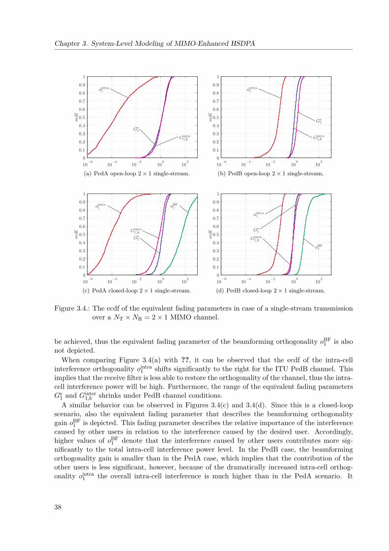
Chapter 3. System-Level Modeling of MIMO-Enhanced HSDPA
10−6
10−4
10−2
100
102
0
0.1
0.2
0.3
0.4
0.5
0.6
0.7
0.8
0.9
1ecdf
(a) PedA open-loop 2× 1 single-stream.10
−610
−410
−210
010
20
0.1
0.2
0.3
0.4
0.5
0.6
0.7
0.8
0.9
1
ecdf
(b) PedB open-loop 2× 1 single-stream.
10−6
10−4
10−2
100
102
0
0.1
0.2
0.3
0.4
0.5
0.6
0.7
0.8
0.9
1
ecdf
(c) PedA closed-loop 2× 1 single-stream.10
−610
−410
−210
010
20
0.1
0.2
0.3
0.4
0.5
0.6
0.7
0.8
0.9
1
ecdf
(d) PedB closed-loop 2× 1 single-stream.
Figure 3.4.: The ecdf of the equivalent fading parameters in case of a single-stream transmissionover a NT ×NR = 2× 1 MIMO channel.
be achieved, thus the equivalent fading parameter of the beamforming orthogonality oBF1 is also
not depicted.When comparing Figure 3.4(a) with ??, it can be observed that the ecdf of the intra-cell
interference orthogonality ointra1 shifts significantly to the right for the ITU PedB channel. This
implies that the receive filter is less able to restore the orthogonality of the channel, thus the intra-cell interference power will be high. Furthermore, the range of the equivalent fading parametersGs
1 and Ginter1,b shrinks under PedB channel conditions.
A similar behavior can be observed in Figures 3.4(c) and 3.4(d). Since this is a closed-loopscenario, also the equivalent fading parameter that describes the beamforming orthogonalitygain oBF
1 is depicted. This fading parameter describes the relative importance of the interferencecaused by other users in relation to the interference caused by the desired user. Accordingly,higher values of oBF
1 denote that the interference caused by other users contributes more sig-nificantly to the total intra-cell interference power level. In the PedB case, the beamformingorthogonality gain is smaller than in the PedA case, which implies that the contribution of theother users is less significant, however, because of the dramatically increased intra-cell orthog-onality ointra
1 the overall intra-cell interference is much higher than in the PedA scenario. It
38
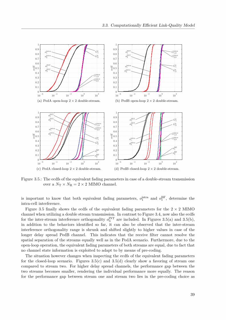
3.3. Computationally Efficient Link-Quality Model
10−6
10−4
10−2
100
102
0
0.1
0.2
0.3
0.4
0.5
0.6
0.7
0.8
0.9
1
ecdf
(a) PedA open-loop 2× 2 double-stream.10
−610
−410
−210
010
20
0.1
0.2
0.3
0.4
0.5
0.6
0.7
0.8
0.9
1
ecdf
(b) PedB open-loop 2× 2 double-stream.
10−6
10−4
10−2
100
102
0
0.1
0.2
0.3
0.4
0.5
0.6
0.7
0.8
0.9
1
ecdf
(c) PedA closed-loop 2× 2 double-stream.10
−610
−410
−210
010
20
0.1
0.2
0.3
0.4
0.5
0.6
0.7
0.8
0.9
1ecdf
(d) PedB closed-loop 2× 2 double-stream.
Figure 3.5.: The ecdfs of the equivalent fading parameters in case of a double-stream transmissionover a NT ×NR = 2× 2 MIMO channel.
is important to know that both equivalent fading parameters, ointra1 and oBF
1 , determine theintra-cell interference.
Figure 3.5 finally shows the ecdfs of the equivalent fading parameters for the 2 × 2 MIMOchannel when utilizing a double stream transmission. In contrast to Figure 3.4, now also the ecdfsfor the inter-stream interference orthogonality oINT
n are included. In Figures 3.5(a) and 3.5(b),in addition to the behaviors identified so far, it can also be observed that the inter-streaminterference orthogonality range is shrunk and shifted slightly to higher values in case of thelonger delay spread PedB channel. This indicates that the receive filter cannot resolve thespatial separation of the streams equally well as in the PedA scenario. Furthermore, due to theopen-loop operation, the equivalent fading parameters of both streams are equal, due to fact thatno channel state information is exploited to adapt to by means of pre-coding.
The situation however changes when inspecting the ecdfs of the equivalent fading parametersfor the closed-loop scenario. Figures 3.5(c) and 3.5(d) clearly show a favoring of stream onecompared to stream two. For higher delay spread channels, the performance gap between thetwo streams becomes smaller, rendering the individual performance more equally. The reasonfor the performance gap between stream one and stream two lies in the pre-coding choice as
39
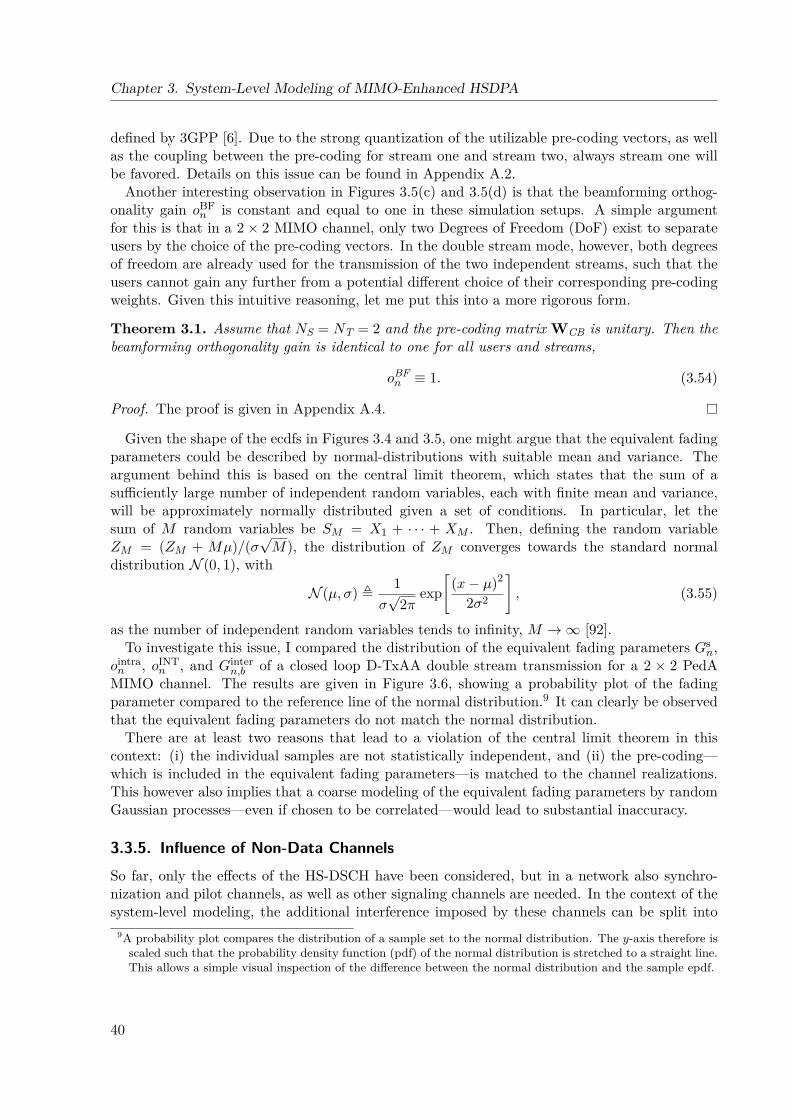
Chapter 3. System-Level Modeling of MIMO-Enhanced HSDPA
defined by 3GPP [6]. Due to the strong quantization of the utilizable pre-coding vectors, as wellas the coupling between the pre-coding for stream one and stream two, always stream one willbe favored. Details on this issue can be found in Appendix A.2.
Another interesting observation in Figures 3.5(c) and 3.5(d) is that the beamforming orthog-onality gain oBF
n is constant and equal to one in these simulation setups. A simple argumentfor this is that in a 2× 2 MIMO channel, only two Degrees of Freedom (DoF) exist to separateusers by the choice of the pre-coding vectors. In the double stream mode, however, both degreesof freedom are already used for the transmission of the two independent streams, such that theusers cannot gain any further from a potential different choice of their corresponding pre-codingweights. Given this intuitive reasoning, let me put this into a more rigorous form.
Theorem 3.1. Assume that NS = NT = 2 and the pre-coding matrix WCB is unitary. Then thebeamforming orthogonality gain is identical to one for all users and streams,
oBFn ≡ 1. (3.54)
Proof. The proof is given in Appendix A.4.
Given the shape of the ecdfs in Figures 3.4 and 3.5, one might argue that the equivalent fadingparameters could be described by normal-distributions with suitable mean and variance. Theargument behind this is based on the central limit theorem, which states that the sum of asufficiently large number of independent random variables, each with finite mean and variance,will be approximately normally distributed given a set of conditions. In particular, let thesum of M random variables be SM = X1 + · · · + XM . Then, defining the random variableZM = (ZM + Mµ)/(σ
√M), the distribution of ZM converges towards the standard normal
distribution N (0, 1), with
N (µ, σ) , 1σ√
2πexp
[(x− µ)2
2σ2
], (3.55)
as the number of independent random variables tends to infinity, M →∞ [92].To investigate this issue, I compared the distribution of the equivalent fading parameters Gs
n,ointran , oINT
n , and Gintern,b of a closed loop D-TxAA double stream transmission for a 2 × 2 PedA
MIMO channel. The results are given in Figure 3.6, showing a probability plot of the fadingparameter compared to the reference line of the normal distribution.9 It can clearly be observedthat the equivalent fading parameters do not match the normal distribution.
There are at least two reasons that lead to a violation of the central limit theorem in thiscontext: (i) the individual samples are not statistically independent, and (ii) the pre-coding—which is included in the equivalent fading parameters—is matched to the channel realizations.This however also implies that a coarse modeling of the equivalent fading parameters by randomGaussian processes—even if chosen to be correlated—would lead to substantial inaccuracy.
3.3.5. Influence of Non-Data ChannelsSo far, only the effects of the HS-DSCH have been considered, but in a network also synchro-nization and pilot channels, as well as other signaling channels are needed. In the context of thesystem-level modeling, the additional interference imposed by these channels can be split into
9A probability plot compares the distribution of a sample set to the normal distribution. The y-axis therefore isscaled such that the probability density function (pdf) of the normal distribution is stretched to a straight line.This allows a simple visual inspection of the difference between the normal distribution and the sample epdf.
40
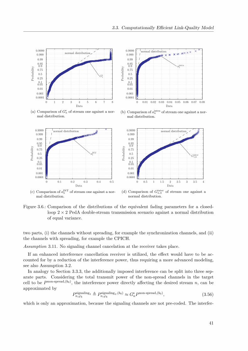
3.3. Computationally Efficient Link-Quality Model
0 1 2 3 4 5 6 7 8
0.00010.001
0.010.050.10.250.50.750.90.950.99
0.9990.9999
Data
Pro
babi
lity
normal distribution
(a) Comparison of Gsn of stream one against a nor-
mal distribution.
0 0.01 0.02 0.03 0.04 0.05 0.06 0.07 0.08
0.00010.001
0.010.050.10.250.50.750.90.950.99
0.9990.9999
Data
Pro
babi
lity
normal distribution
(b) Comparison of ointran of stream one against a nor-
mal distribution.
0 0.1 0.2 0.3 0.4 0.5
0.00010.001
0.010.050.10.250.50.750.90.950.99
0.9990.9999
Data
Pro
babi
lity
normal distribution
(c) Comparison of oINTn of stream one against a nor-
mal distribution.
0 0.5 1 1.5 2 2.5 3 3.5 4
0.00010.001
0.010.050.10.250.50.750.90.950.99
0.9990.9999
Data
Pro
babi
lity
normal distribution
(d) Comparison of Gintern,b of stream one against a
normal distribution.
Figure 3.6.: Comparison of the distributions of the equivalent fading parameters for a closed-loop 2× 2 PedA double-stream transmission scenario against a normal distributionof equal variance.
two parts, (i) the channels without spreading, for example the synchronization channels, and (ii)the channels with spreading, for example the CPICH.
Assumption 3.11. No signaling channel cancelation at the receiver takes place.
If an enhanced interference cancellation receiver is utilized, the effect would have to be ac-counted for by a reduction of the interference power, thus requiring a more advanced modeling,see also Assumption 3.2.
In analogy to Section 3.3.3, the additionally imposed interference can be split into three sep-arate parts. Considering the total transmit power of the non-spread channels in the targetcell to be P non-spread,(b0), the interference power directly affecting the desired stream n, can beapproximated by
P signaling1n,ϕk
, P signaling1,(b0)n,ϕk
≈ GsnP
non-spread,(b0), (3.56)
which is only an approximation, because the signaling channels are not pre-coded. The interfer-
41

Chapter 3. System-Level Modeling of MIMO-Enhanced HSDPA
ence power added on top of all other streams, which are again interfering with the desired streamis
P signaling2n,ϕk
, P signaling2,(b0)n,ϕk
≈NS∑m=0m6=n
oINTn P non-spread,(b0), (3.57)
and the remaining inter-symbol and inter-code interference can be evaluated to be
P signaling3n,ϕk
, P signaling3,(b0)n,ϕk
≈ ointran Gs
nPnon-spread,(b0). (3.58)
Adding these individual parts, the total interference caused by the non-spread signaling channelis given by
3∑i=1
P signalingin,ϕk
≈ P non-spread,(b0)
Gsn
(1 + ointra
n
)+
NS∑m=0m 6=n
oINTn
. (3.59)
The interference caused by other spread channels can be treated similarly to the intra-cellinterference, caused by loss of spreading code orthogonality. Assuming the total power of otherspread channels in the cell to be P spread,(b0), the interference can be evaluated to be
P signaling4n,ϕk
, P signaling4,(b0)n,ϕk
≈ ointran Gs
nPspread,(b0), (3.60)
and accordingly, the total signaling interference power becomes
P signalingn,ϕk
=4∑i=1
P signalingin,ϕk
= P non-spread,(b0)
Gsn
(1 + ointra
n
)+
NS∑m=0m 6=n
oINTn
+ ointran Gs
nPspread,(b0).
(3.61)
3.3.6. Resulting SINR DescriptionWith these findings, the SINR on stream n and spreading code ϕk, as observed after equalizationand despreading,10 can be expressed as
SINRn,ϕk =SF · P s
n,ϕk1
L(b0)(SF · P INT
n,ϕk+ P intra
n,ϕk+ P signaling
n,ϕk
)1
L(b0) +∑B
b=1b 6=b0
Gintern,b P
(b) 1L(b) + P noise
, (3.62)
where SF denotes the spreading factor of the HSDPA data channels. The term 1L(b) represents
the macro-scale and shadow-fading path-loss components of the MIMO channel in the networkcontext. Details about the composition and the modeling of this term will be given in Section 4.1.For D-TxAA HSDPA in particular, the inter-stream interference power P INT
n,ϕkin Equation (3.62)
simplifies toP INTn,ϕk
= oINT¬n P
(u0,b0)¬n,ϕ(¬n)
k
, (3.63)
where ¬n denotes the opposite stream of stream n.The description contains only equivalent fading parameters and power terms, which do not
depend on each other. Accordingly, traces for the fading parameters may be generated prior10Also often called symbol-level SINR.
42
3.3. Computationally Efficient Link-Quality Model
to the system-level simulation, and thus only real-valued scalar multiplications will occur inEquation (3.62) when evaluated on system-level. It is also worth noticing that in principle onlyone trace for each equivalent fading parameter has to be generated, statistical independencebetween different realizations for different users can always be achieved by choosing independentstarting indices, for example drawn uniformly over the length of the respective trace. However, ifsuch an implementation is desired, the equivalent fading parameter traces have to be interpretedas a loop trace, which means that when the current index within the trace reaches its end, itwill start from the beginning of the trace again. The index pointing to the current position inthe trace thus has to be taken modulo the length of the trace. To avoid edge-effects when thetrace index jumps from the end to the beginning, some sort of smoothing has to be performed,for example by linear interpolation.
Furthermore, although I only applied ITU channel profiles in this work, I want to point outthat the proposed structure can be utilized for arbitrary channel models, like the Spatial ChannelModel (SCM) or the Spatial Channel Model Extended (SCME) [93].
3.3.7. ValidationTo show that the proposed link-quality model can accurately approximate the SINR for variousoperation modes of the physical layer, I conducted a set of link-level simulations. For this purpose,a physical-layer simulator was developed [21], to compare the true SINR with the SINR predictedby the model in Equation (3.62). The basic functionality of the physical-layer simulator is builton parts of the implementation of [94] with some necessary adaptions.
The utilized MIMO HSDPA physical-layer simulator emulates the transmission of the shareduser-data channel HS-DSCH and the pilot channel(s) CPICH. The bit sequences in the simulatorflow are encapsulated in TTIs of 2 ms each, as explained in Chapter 2. The channel modelimplemented is generating block-fading channel realizations on a TTI basis, using the Rayleighfading generator of [8, 91]. For the validation simulations, however, some restrictions apply, inparticular
• channel estimation is not taken into account, thus full CSI is assumed at the receiver,• large-scale and shadow fading issues are not taken into account,11 and• inter-cell interference is not considered in the simulation.
Although these are restrictive assumptions, still the inter-stream and intra-cell interference mod-eling accuracy can be assessed very well.
Since Equation (3.62) predicts the SINR after equalization and de-spreading, the values ob-tained by the model with the true SINR have to be compared. By defining the de-spread symbolof the transmit chips for stream n utilizing spreading-code ϕk,
s(n,ϕk) = ϕ(n)k
x(n,ϕk)
, (3.64)
where I omitted the time indices for sake of notational simplicity, the true SINR is given byevaluating
SINRtruen,ϕk
,E∥∥∥s(n,ϕk)g(n)
∥∥∥2
E∥∥s(n,ϕk)g(n) − s(n,ϕk)
∥∥2 , (3.65)
11Note that these terms will be explained in more detail in the context of the system-level simulator in Section 4.1.
43
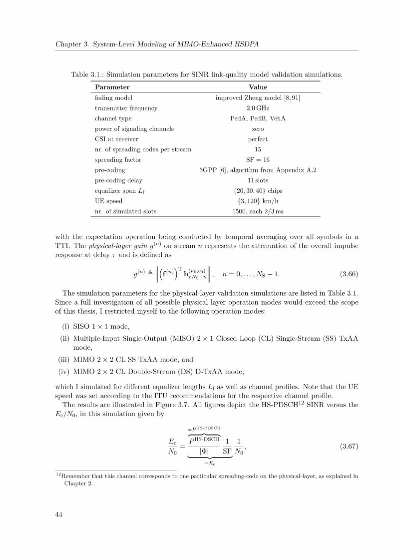
Chapter 3. System-Level Modeling of MIMO-Enhanced HSDPA
Table 3.1.: Simulation parameters for SINR link-quality model validation simulations.Parameter Valuefading model improved Zheng model [8, 91]transmitter frequency 2.0 GHzchannel type PedA, PedB, VehApower of signaling channels zeroCSI at receiver perfectnr. of spreading codes per stream 15spreading factor SF = 16pre-coding 3GPP [6], algorithm from Appendix A.2pre-coding delay 11 slotsequalizer span Lf 20, 30, 40 chipsUE speed 3, 120 km/hnr. of simulated slots 1500, each 2/3 ms
with the expectation operation being conducted by temporal averaging over all symbols in aTTI. The physical-layer gain g(n) on stream n represents the attenuation of the overall impulseresponse at delay τ and is defined as
g(n) ,∥∥∥∥(f (n)
)Th(u0,b0)τNS+n
∥∥∥∥ , n = 0, . . . , NS − 1. (3.66)
The simulation parameters for the physical-layer validation simulations are listed in Table 3.1.Since a full investigation of all possible physical layer operation modes would exceed the scopeof this thesis, I restricted myself to the following operation modes:
(i) SISO 1× 1 mode,(ii) Multiple-Input Single-Output (MISO) 2 × 1 Closed Loop (CL) Single-Stream (SS) TxAA
mode,(iii) MIMO 2× 2 CL SS TxAA mode, and(iv) MIMO 2× 2 CL Double-Stream (DS) D-TxAA mode,
which I simulated for different equalizer lengths Lf as well as channel profiles. Note that the UEspeed was set according to the ITU recommendations for the respective channel profile.
The results are illustrated in Figure 3.7. All figures depict the HS-PDSCH12 SINR versus theEc/N0, in this simulation given by
EcN0
=
=PHS-PDSCH︷ ︸︸ ︷PHS-DSCH
|Φ|1
SF︸ ︷︷ ︸=Ec
1N0
, (3.67)
12Remember that this channel corresponds to one particular spreading-code on the physical-layer, as explained inChapter 2.
44
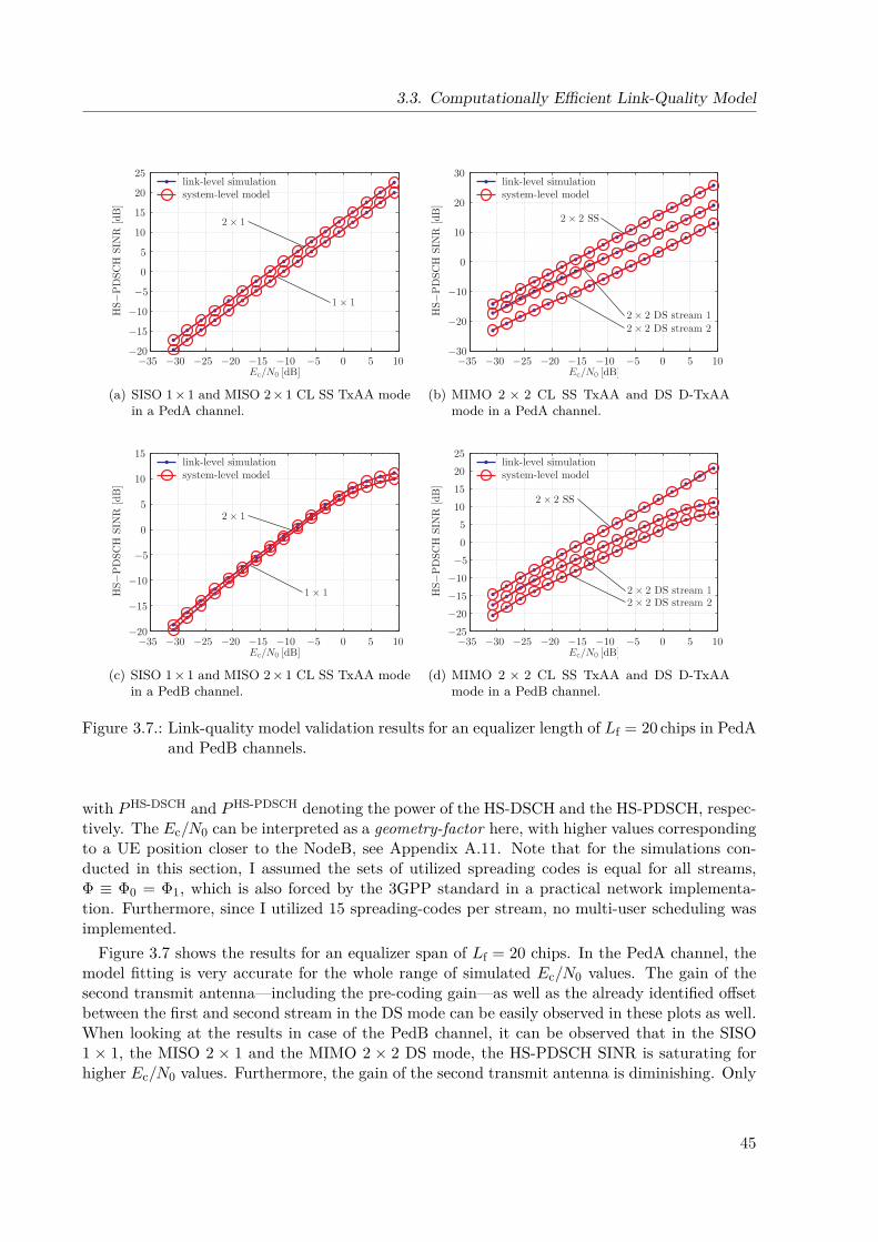
3.3. Computationally Efficient Link-Quality Model
−35 −30 −25 −20 −15 −10 −5 0 5 10−20
−15
−10
−5
0
5
10
15
20
25
HS−
PD
SCH
SIN
R [dB
]
link-level simulationsystem-level model
(a) SISO 1× 1 and MISO 2× 1 CL SS TxAA modein a PedA channel.
−35 −30 −25 −20 −15 −10 −5 0 5 10−30
−20
−10
0
10
20
30
HS−
PD
SCH
SIN
R [dB
]
link-level simulationsystem-level model
(b) MIMO 2 × 2 CL SS TxAA and DS D-TxAAmode in a PedA channel.
−35 −30 −25 −20 −15 −10 −5 0 5 10−20
−15
−10
−5
0
5
10
15
HS−
PD
SCH
SIN
R [dB
]
link-level simulationsystem-level model
(c) SISO 1× 1 and MISO 2× 1 CL SS TxAA modein a PedB channel.
−35 −30 −25 −20 −15 −10 −5 0 5 10−25
−20
−15
−10
−5
0
5
10
15
20
25
HS−
PD
SCH
SIN
R [dB
]
link-level simulationsystem-level model
(d) MIMO 2 × 2 CL SS TxAA and DS D-TxAAmode in a PedB channel.
Figure 3.7.: Link-quality model validation results for an equalizer length of Lf = 20 chips in PedAand PedB channels.
with PHS-DSCH and PHS-PDSCH denoting the power of the HS-DSCH and the HS-PDSCH, respec-tively. The Ec/N0 can be interpreted as a geometry-factor here, with higher values correspondingto a UE position closer to the NodeB, see Appendix A.11. Note that for the simulations con-ducted in this section, I assumed the sets of utilized spreading codes is equal for all streams,Φ ≡ Φ0 = Φ1, which is also forced by the 3GPP standard in a practical network implementa-tion. Furthermore, since I utilized 15 spreading-codes per stream, no multi-user scheduling wasimplemented.
Figure 3.7 shows the results for an equalizer span of Lf = 20 chips. In the PedA channel, themodel fitting is very accurate for the whole range of simulated Ec/N0 values. The gain of thesecond transmit antenna—including the pre-coding gain—as well as the already identified offsetbetween the first and second stream in the DS mode can be easily observed in these plots as well.When looking at the results in case of the PedB channel, it can be observed that in the SISO1 × 1, the MISO 2 × 1 and the MIMO 2 × 2 DS mode, the HS-PDSCH SINR is saturating forhigher Ec/N0 values. Furthermore, the gain of the second transmit antenna is diminishing. Only
45
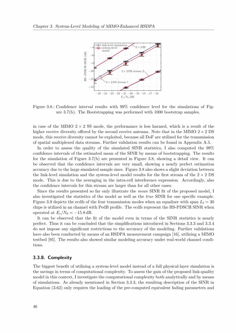
Chapter 3. System-Level Modeling of MIMO-Enhanced HSDPA
−25 −24 −23 −22 −21 −20 −19 −18 −17 −16
−14
−12
−10
−8
−6
−4
HS−
PD
SCH
SIN
R [dB
]
link-level simulationsystem-levelmodel
Figure 3.8.: Confidence interval results with 99% confidence level for the simulations of Fig-ure 3.7(b). The Bootstrapping was performed with 1000 bootstrap samples.
in case of the MIMO 2 × 2 SS mode, the performance is less harmed, which is a result of thehigher receive diversity offered by the second receive antenna. Note that in the MIMO 2× 2 DSmode, this receive diversity cannot be exploited, because all DoF are utilized for the transmissionof spatial multiplexed data streams. Further validation results can be found in Appendix A.5.
In order to assess the quality of the simulated SINR statistics, I also computed the 99%confidence intervals of the estimated mean of the SINR by means of bootstrapping. The resultsfor the simulation of Figure 3.7(b) are presented in Figure 3.8, showing a detail view. It canbe observed that the confidence intervals are very small, showing a nearly perfect estimationaccuracy due to the large simulated sample sizes. Figure 3.8 also shows a slight deviation betweenthe link-level simulation and the system-level model results for the first stream of the 2× 2 DSmode. This is due to the averaging in the intra-cell interference expression. Accordingly, alsothe confidence intervals for this stream are larger than for all other cases.
Since the results presented so far only illustrate the mean SINR fit of the proposed model, Ialso investigated the statistics of the model as well as the true SINR for one specific example.Figure 3.9 depicts the ecdfs of the four transmission modes when an equalizer with span Lf = 30chips is utilized in an channel with PedB profile. The ecdfs represent the HS-PDSCH SINR whenoperated at Ec/N0 = −15.8 dB.
It can be observed that the fit of the model even in terms of the SINR statistics is nearlyperfect. Thus it can be concluded that the simplifications introduced in Sections 3.3.3 and 3.3.4do not impose any significant restrictions to the accuracy of the modeling. Further validationshave also been conducted by means of an HSDPA measurement campaign [16], utilizing a MIMOtestbed [95]. The results also showed similar modeling accuracy under real-world channel condi-tions.
3.3.8. Complexity
The biggest benefit of utilizing a system-level model instead of a full physical-layer simulation isthe savings in terms of computational complexity. To assess the gain of the proposed link-qualitymodel in this context, I investigate the computational complexity both analytically and by meansof simulations. As already mentioned in Section 3.3.3, the resulting description of the SINR inEquation (3.62) only requires the loading of the pre-computed equivalent fading parameters and
46
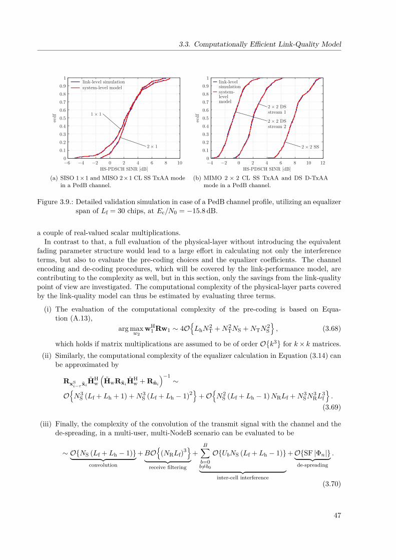
3.3. Computationally Efficient Link-Quality Model
−6 −4 −2 0 2 4 6 8 100
0.1
0.2
0.3
0.4
0.5
0.6
0.7
0.8
0.9
1
HS-PDSCH SINR [dB]
ecdf
link-level simulationsystem-level model
(a) SISO 1×1 and MISO 2×1 CL SS TxAA modein a PedB channel.
−4 −2 0 2 4 6 8 10 120
0.1
0.2
0.3
0.4
0.5
0.6
0.7
0.8
0.9
1
HS-PDSCH SINR [dB]
ecdf
link-levelsimulationsystem-levelmodel
stream 1
stream 2
(b) MIMO 2 × 2 CL SS TxAA and DS D-TxAAmode in a PedB channel.
Figure 3.9.: Detailed validation simulation in case of a PedB channel profile, utilizing an equalizerspan of Lf = 30 chips, at Ec/N0 = −15.8 dB.
a couple of real-valued scalar multiplications.In contrast to that, a full evaluation of the physical-layer without introducing the equivalent
fading parameter structure would lead to a large effort in calculating not only the interferenceterms, but also to evaluate the pre-coding choices and the equalizer coefficients. The channelencoding and de-coding procedures, which will be covered by the link-performance model, arecontributing to the complexity as well, but in this section, only the savings from the link-qualitypoint of view are investigated. The computational complexity of the physical-layer parts coveredby the link-quality model can thus be estimated by evaluating three terms.
(i) The evaluation of the computational complexity of the pre-coding is based on Equa-tion (A.13),
arg maxw2
wH1 Rw1 ∼ 4O
LhN
2T +N2
TNS +NTN2S
, (3.68)
which holds if matrix multiplications are assumed to be of order Ok3 for k× k matrices.
(ii) Similarly, the computational complexity of the equalizer calculation in Equation (3.14) canbe approximated by
RxSi−τ xiH
Hw
(HwRxiHH
w + Rni
)−1∼
ON3
S (Lf + Lh + 1) +N3S (Lf + Lh − 1)2
+O
N2
S (Lf + Lh − 1)NRLf +N3SN
3RL
3f
.
(3.69)
(iii) Finally, the complexity of the convolution of the transmit signal with the channel and thede-spreading, in a multi-user, multi-NodeB scenario can be evaluated to be
∼ ONS (Lf + Lh − 1)︸ ︷︷ ︸convolution
+BO
(NRLf)3
︸ ︷︷ ︸receive filtering
+B∑b=0b6=b0
OUbNS (Lf + Lh − 1)
︸ ︷︷ ︸inter-cell interference
+OSF |Φn|︸ ︷︷ ︸de-spreading
.
(3.70)
47
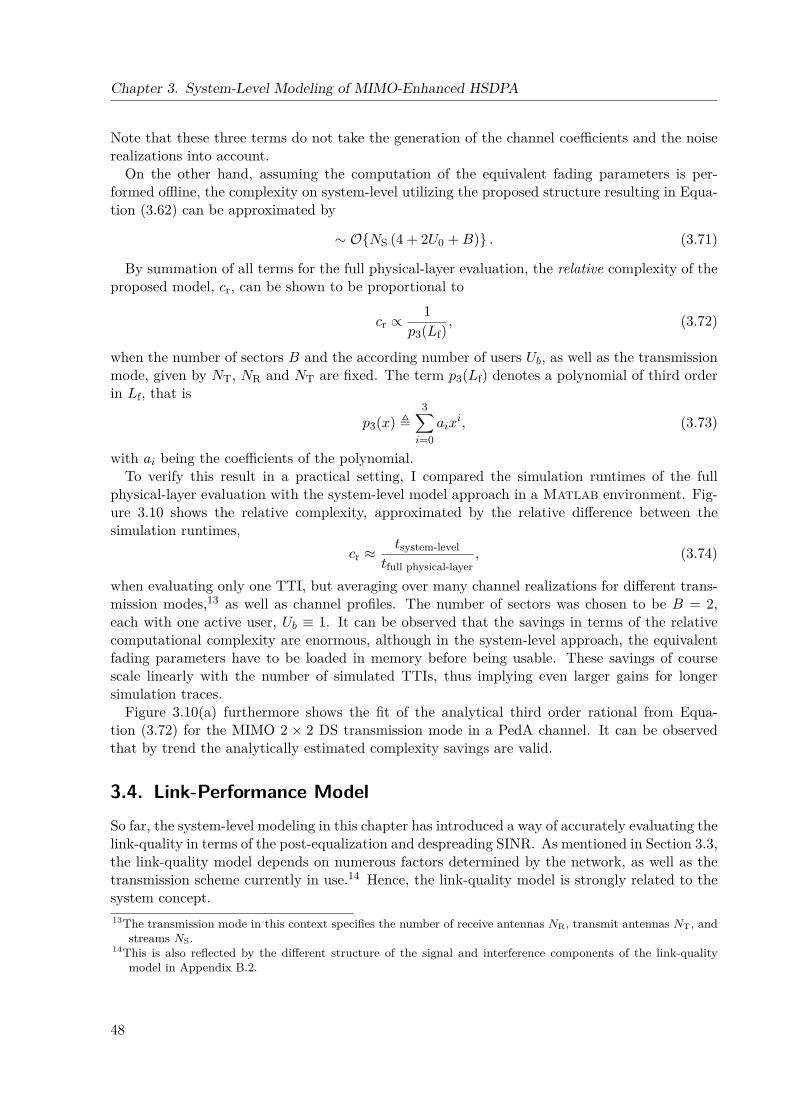
Chapter 3. System-Level Modeling of MIMO-Enhanced HSDPA
Note that these three terms do not take the generation of the channel coefficients and the noiserealizations into account.
On the other hand, assuming the computation of the equivalent fading parameters is per-formed offline, the complexity on system-level utilizing the proposed structure resulting in Equa-tion (3.62) can be approximated by
∼ ONS (4 + 2U0 +B) . (3.71)
By summation of all terms for the full physical-layer evaluation, the relative complexity of theproposed model, cr, can be shown to be proportional to
cr ∝1
p3(Lf), (3.72)
when the number of sectors B and the according number of users Ub, as well as the transmissionmode, given by NT, NR and NT are fixed. The term p3(Lf) denotes a polynomial of third orderin Lf, that is
p3(x) ,3∑i=0
aixi, (3.73)
with ai being the coefficients of the polynomial.To verify this result in a practical setting, I compared the simulation runtimes of the full
physical-layer evaluation with the system-level model approach in a Matlab environment. Fig-ure 3.10 shows the relative complexity, approximated by the relative difference between thesimulation runtimes,
cr ≈tsystem-level
tfull physical-layer, (3.74)
when evaluating only one TTI, but averaging over many channel realizations for different trans-mission modes,13 as well as channel profiles. The number of sectors was chosen to be B = 2,each with one active user, Ub ≡ 1. It can be observed that the savings in terms of the relativecomputational complexity are enormous, although in the system-level approach, the equivalentfading parameters have to be loaded in memory before being usable. These savings of coursescale linearly with the number of simulated TTIs, thus implying even larger gains for longersimulation traces.
Figure 3.10(a) furthermore shows the fit of the analytical third order rational from Equa-tion (3.72) for the MIMO 2 × 2 DS transmission mode in a PedA channel. It can be observedthat by trend the analytically estimated complexity savings are valid.
3.4. Link-Performance ModelSo far, the system-level modeling in this chapter has introduced a way of accurately evaluating thelink-quality in terms of the post-equalization and despreading SINR. As mentioned in Section 3.3,the link-quality model depends on numerous factors determined by the network, as well as thetransmission scheme currently in use.14 Hence, the link-quality model is strongly related to thesystem concept.13The transmission mode in this context specifies the number of receive antennas NR, transmit antennas NT, and
streams NS.14This is also reflected by the different structure of the signal and interference components of the link-quality
model in Appendix B.2.
48
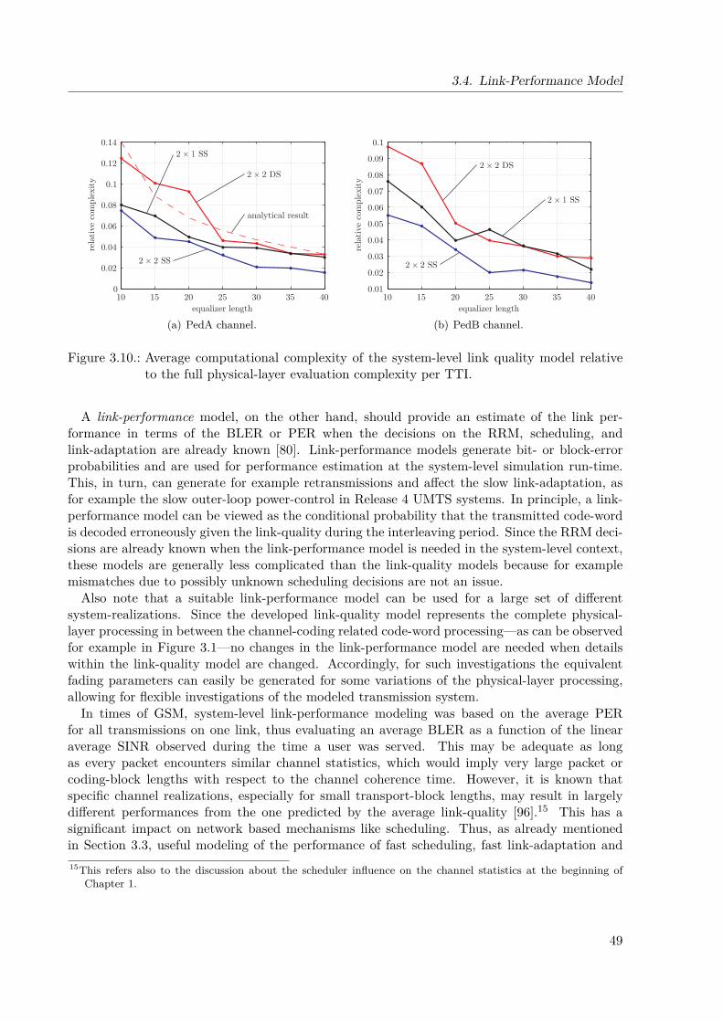
3.4. Link-Performance Model
10 15 20 25 30 35 400
0.02
0.04
0.06
0.08
0.1
0.12
0.14
equalizer length
rela
tive
com
plex
ity
analytical result
(a) PedA channel.
10 15 20 25 30 35 400.01
0.02
0.03
0.04
0.05
0.06
0.07
0.08
0.09
0.1
equalizer length
rela
tive
com
plex
ity
(b) PedB channel.
Figure 3.10.: Average computational complexity of the system-level link quality model relativeto the full physical-layer evaluation complexity per TTI.
A link-performance model, on the other hand, should provide an estimate of the link per-formance in terms of the BLER or PER when the decisions on the RRM, scheduling, andlink-adaptation are already known [80]. Link-performance models generate bit- or block-errorprobabilities and are used for performance estimation at the system-level simulation run-time.This, in turn, can generate for example retransmissions and affect the slow link-adaptation, asfor example the slow outer-loop power-control in Release 4 UMTS systems. In principle, a link-performance model can be viewed as the conditional probability that the transmitted code-wordis decoded erroneously given the link-quality during the interleaving period. Since the RRM deci-sions are already known when the link-performance model is needed in the system-level context,these models are generally less complicated than the link-quality models because for examplemismatches due to possibly unknown scheduling decisions are not an issue.
Also note that a suitable link-performance model can be used for a large set of differentsystem-realizations. Since the developed link-quality model represents the complete physical-layer processing in between the channel-coding related code-word processing—as can be observedfor example in Figure 3.1—no changes in the link-performance model are needed when detailswithin the link-quality model are changed. Accordingly, for such investigations the equivalentfading parameters can easily be generated for some variations of the physical-layer processing,allowing for flexible investigations of the modeled transmission system.
In times of GSM, system-level link-performance modeling was based on the average PERfor all transmissions on one link, thus evaluating an average BLER as a function of the linearaverage SINR observed during the time a user was served. This may be adequate as longas every packet encounters similar channel statistics, which would imply very large packet orcoding-block lengths with respect to the channel coherence time. However, it is known thatspecific channel realizations, especially for small transport-block lengths, may result in largelydifferent performances from the one predicted by the average link-quality [96].15 This has asignificant impact on network based mechanisms like scheduling. Thus, as already mentionedin Section 3.3, useful modeling of the performance of fast scheduling, fast link-adaptation and15This refers also to the discussion about the scheduler influence on the channel statistics at the beginning of
Chapter 1.
49
Chapter 3. System-Level Modeling of MIMO-Enhanced HSDPA
link-
qual
ity
mod
el
map
ping
/com
pres
sion
AW
GN
bas
ed P
ER
pre
dict
ionphysical
layerparameters
channel
networkparameters
BLER
link-performance model
Figure 3.11.: Basic concept of the proposed link-performance model, including the input param-eter generation by the link-quality model. The mapping/compression depends onthe symbol alphabet A, as well as a vector of tuning parameters β. Similarly, theAWGN based PER prediction depends on the symbol alphabet and the coding raterc of the current transmission, constituting the transmit CQI c(T).
HARQ is impossible with average or large-scale parameters and accordingly small-scale effectshave to be included.
3.4.1. Link-Performance Model ConceptThe basic structure of the proposed link-performance model and its connection to the proposedlink-quality model is depicted in Figure 3.11. The principal idea follows the framework of [80,84]which I adapted to the needs of MIMO HSDPA.
As illustrated, the link quality model provides small-scale fading dependent link-quality esti-mates, SINRn,ϕk , given by Equation (3.62). Note that, as explained in Chapter 2, the packet unitin HSDPA is given by a sub-frame or transport block with the length of one TTI. A straightfor-ward approach would thus be to evaluate the link-quality once every TTI and utilize the resultingmeasurements as input parameters to the link-performance model. If, however, the link-qualitychanges significantly during one sub-frame, a link-performance model utilizing TTI based SINRsampling—corresponding to an average SINR evaluation for every sub-frame—would not reflectthese variations and thus probably lead to too optimistic performance predictions. Such a situa-tion would occur in a scenario where the users are moving or the channel varies due to changesin the environment.
To overcome this problem, I propose to conduct an oversampling in terms of the link-qualitymodel estimates, thus evaluating SINRn,ϕk more than once per sub-frame. In particular, I suggestto evaluate the SINR on a slot basis, that is three times per TTI,
SINR(i)n,ϕk
, i = 1, 2, 3, (3.75)
with i denoting the relative time index within one TTI. This obviously allows for an increasedaccuracy in movement scenarios.16
16To estimate the maximum speed that can be covered accurately by this link-quality model sampling rate, let
50
3.4. Link-Performance Model
Given the slot-sampled link-quality model estimations, the link-performance model has toestimate the link performance in terms of the ACK/NACK report for the individual transportblock. In principle, the best—in terms of accuracy—link-performance model approach wouldbe to utilize a multi-dimensional mapping that directly converts the SINRs to the anticipatedBLER,
SINR(i)n,ϕk7→ BLER, (3.76)
but this would require analytic models of very high complexity, or unfeasible large look-up tables.A more suitable way of representing the information contained in the sampled link-quality modeldata is to compress the input parameters to a few effective link-quality parameters. Recent workon that subject tries to extract potential gains in accuracy by mapping the input parameters totwo-dimensional output data [99], for example given by the average SINR as well as the varianceof the estimated SINR values.
For this thesis, I utilized a compression mapping that results in an one-dimensional effectiveSINR per spatial stream, SINReff
n . The idea for the representation of the link-performance interms of an effective SINR was already proposed in [100], but has not been used for system-level modeling at that time. Let me denote the mapping/compression stage of the proposedlink-performance model in Figure 3.11 by
fM(A,β) : SINR(i)n,ϕk7→ SINReff
n , (3.77)
with A and β denoting the utilized symbol alphabet for the transmission of the current transportblock and a vector of tuning parameters, respectively. Note that the HSDPA link-adaptationdoes not allow for a change of the symbol alphabet within a transport block.
The mapping function fM(A,β) that turned out to be the best in terms of accuracy andflexibility was the so-called Mutual Information Effective Signal to Interference and Noise RatioMapping (MIESM). This mapping has initially been proposed in the Radio Access Network(RAN) working meetings of 3GPP [101], and builds upon the Bit-Interleaved Coded Modulation(BICM) capacity as identified in [102],17
I(x) = log2 |A| − Ey
1|A|
log2|A|∑d=1
1∑b=0
∑z∈A(d)
b
log∑x∈A exp
[− |y −
√x (x− z)|2
]∑x∈A(d)
b
exp[− |y −
√x (x− z)|2
] , (3.78)
with |A| denoting the cardinality of the symbol alphabet A, y being a zero mean unit variancecomplex Gaussian variable and A(d)
b denoting the set of symbols for which bit d equals b. Theresulting mutual information curves in comparison to the Shannon capacity are depicted in
me apply the Jakes model [97]. It is well known [49] that the channel coherence TC time can be approximatedas a function of the Doppler spread, DS, that is TC ≈ 1/DS. Assuming a Doppler power spectral densityas derived by Jakes, the Doppler spread can be approximated by DS ≈ 2fs,max, with fs,max denoting themaximum Doppler frequency shift relative to the carrier frequency fc. This is not always fulfilled in practice,but is a reasonable approximation [98]. The maximum Doppler frequency shift can be calculated according tofs,max = fcv/c0, with v denoting the relative speed of the transmitter/receiver and the scatterers, and c0 beingthe light speed. Accordingly, the maximum v to result in a channel coherence time, less than one slot durationof 2/3 ms is approximately 31.25 km/h. Considering that the target scenario of HSDPA is static this seems tobe sufficient for most investigation scenarios.
17A list of other mapping functions can be found in [80], including for example the well-known ExponentialEffective Signal to Interference and Noise Ratio Mapping (EESM). For GSM, some of the proposed mappingfunctions were based on the so-called raw bit-error probability [103], but was shown to be of less accuracy thanother methods [80].
51
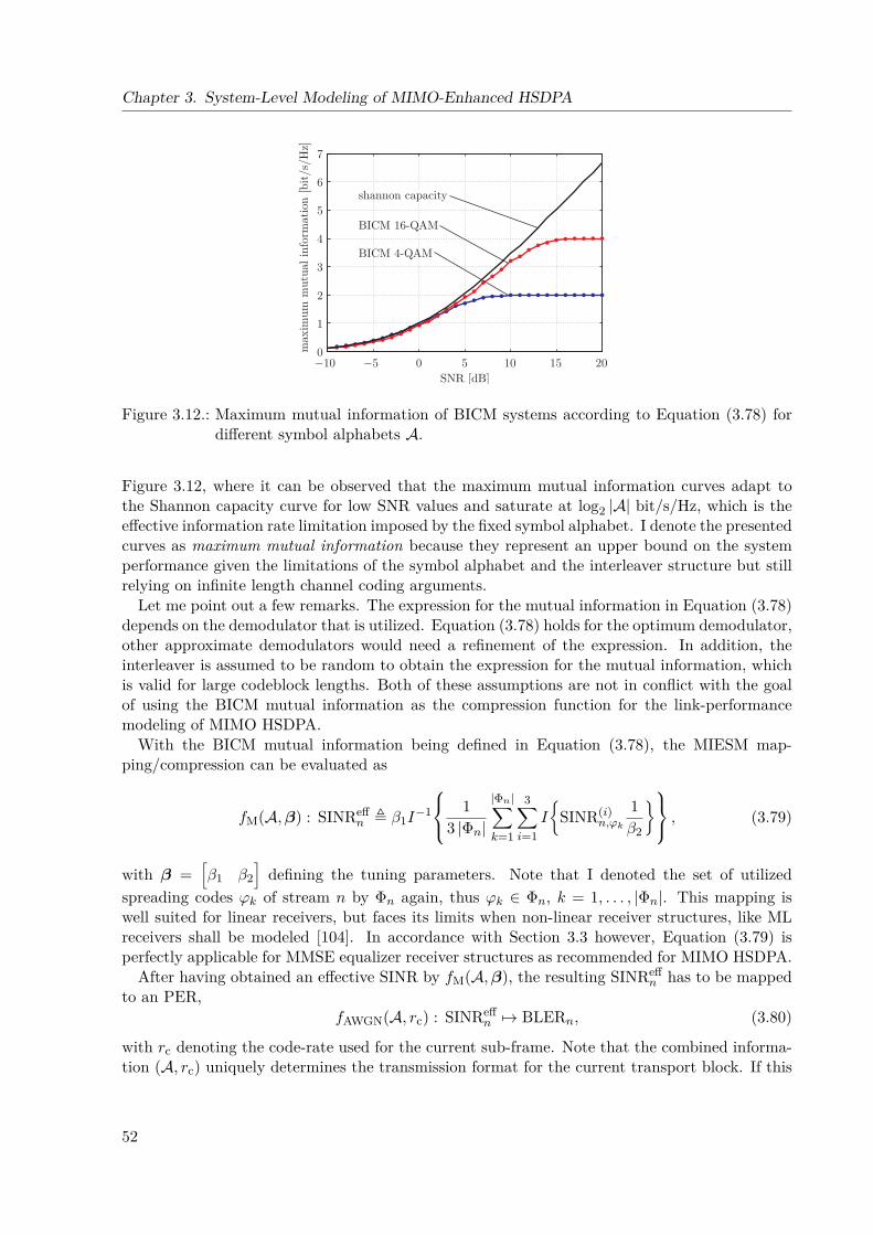
Chapter 3. System-Level Modeling of MIMO-Enhanced HSDPA
−10 −5 0 5 10 15 200
1
2
3
4
5
6
7
SNR [dB]
max
imum
mut
ual in
form
atio
n [b
it/s
/Hz]
shannon capacity
BICM 4-QAM
BICM 16-QAM
Figure 3.12.: Maximum mutual information of BICM systems according to Equation (3.78) fordifferent symbol alphabets A.
Figure 3.12, where it can be observed that the maximum mutual information curves adapt tothe Shannon capacity curve for low SNR values and saturate at log2 |A| bit/s/Hz, which is theeffective information rate limitation imposed by the fixed symbol alphabet. I denote the presentedcurves as maximum mutual information because they represent an upper bound on the systemperformance given the limitations of the symbol alphabet and the interleaver structure but stillrelying on infinite length channel coding arguments.
Let me point out a few remarks. The expression for the mutual information in Equation (3.78)depends on the demodulator that is utilized. Equation (3.78) holds for the optimum demodulator,other approximate demodulators would need a refinement of the expression. In addition, theinterleaver is assumed to be random to obtain the expression for the mutual information, whichis valid for large codeblock lengths. Both of these assumptions are not in conflict with the goalof using the BICM mutual information as the compression function for the link-performancemodeling of MIMO HSDPA.
With the BICM mutual information being defined in Equation (3.78), the MIESM map-ping/compression can be evaluated as
fM(A,β) : SINReffn , β1I
−1
13 |Φn|
|Φn|∑k=1
3∑i=1
I
SINR(i)
n,ϕk
1β2
, (3.79)
with β =[β1 β2
]defining the tuning parameters. Note that I denoted the set of utilized
spreading codes ϕk of stream n by Φn again, thus ϕk ∈ Φn, k = 1, . . . , |Φn|. This mapping iswell suited for linear receivers, but faces its limits when non-linear receiver structures, like MLreceivers shall be modeled [104]. In accordance with Section 3.3 however, Equation (3.79) isperfectly applicable for MMSE equalizer receiver structures as recommended for MIMO HSDPA.
After having obtained an effective SINR by fM(A,β), the resulting SINReffn has to be mapped
to an PER,fAWGN(A, rc) : SINReff
n 7→ BLERn, (3.80)
with rc denoting the code-rate used for the current sub-frame. Note that the combined informa-tion (A, rc) uniquely determines the transmission format for the current transport block. If this
52
3.4. Link-Performance Model
transmission format corresponds to a configuration as defined in the CQI table, I will refer to thecombined information as transmission CQI, c(T) ∼ (A, rc), as already illustrated in Figure 3.11.Details about the CQI tables can be found in Chapter 2.
In the context of this work, I decided to utilize AWGN performance curves as the mappingfrom the effective SINR to BLER. This approach is well-known in the literature [80,84,104], andhas proven to be accurate and robust in terms of applicability for many different transmissionscenarios. The fact that the HSDPA link-adaptation works on a sub-frame basis eases themodeling again at this point, because no AWGN performance curves with mixed transmissionformats are needed.
The AWGN based mapping fAWGN(A, rc) can be acquired by training, meaning a set of AWGNlink-level simulations for the corresponding channel-coding and rate-matching, or by analyticapproximations. Such analytic approximations usually base upon the cut-off rate of the channel,like in [105], which I also applied in Appendix B.1. For the sake of modeling the link-performancefor MIMO enhanced HSDPA, however, I relied on a training based mapping. Thus a set of link-level simulations—for every possible transmission format c(T)—forms a look-up table that isutilized as mapping function fAWGN(A, rc).
Since the link-quality model, as well as the mapping/compression fM(A,β) evaluate sep-arate performance parameters for every spatial data stream,18 the defined BLER mappingfAWGN(A, rc) can be trained by single-stream scenarios and used independently for the trans-mitted code-words, n = 0, . . . , NS − 1.
To finally obtain a sub-frame based ACK/NACK decision that consequently can trigger re-transmissions and influences the scheduler, the output BLER of fM(A,β) is mapped to a packet-error event by conducting a binary random experiment with appropriate probability distribution,
ξ =
0→ ACK : Prξ = 0 = 1− BLER,1→ NACK : Prξ = 1 = BLER.
(3.81)
This guarantees that the BLER values predicted by the link-performance model are obtained inaverage.
3.4.2. Training and Validation of the ModelWith the mapping function being specified by Equation (3.79), it remains to train the model byfinding the optimum parameter vector βopt, and to validate the link-performance model in termsof its BLER prediction error.
For the training, I conducted a set of link-level simulations utilizing the HSDPA physical-layersimulator of [94] for different transmission formats. The simulator is a WCDMA, 3GPP Release 5standard compliant HSDPA simulator that models the complete physical layer. For the trainingof the MIESM, the simulator was configured to vary the Ior/Ioc ratio,19 which can be translatedto a variation in the post-equalization and despreading SINR per HS-PDSCH,
SINRHS-PDSCH ≈ SF IorIoc
EcIor
1|Φ| . (3.82)
This implicitly assumes an average downlink wireless channel gain of one. As explained in theprevious subsection, only single-stream SISO simulations are necessary to be able to derive sep-arate link-performance models for every spatial stream—which can be interpreted as individual18This is possible due to the independent channel-coding of the streams, as already mentioned.19See Appendix A.11 for the corresponding definitions.
53
Chapter 3. System-Level Modeling of MIMO-Enhanced HSDPA
point to point rank one transmission—thus the number of spreading codes used for the currenttransmission is given by the cardinality |Φ|, where I left the index n for the sake of notationalclarity. The instantaneous HS-PDSCH SINR per TTI, needed for the training of the MIESM,however, was extracted from the receive symbols for every received sub-frame, similar to Equa-tion (3.65).
Varying over Ior/Ioc, the physical-layer simulator was utilized to generate a large numberof channel realizations and assess the decoding performance for all of those. The fraction oferroneous received packets within a set of channel realizations then approximates the BLER fora given channel condition,
BLERMc ≈
nr. of NACKstotal nr. of channel realizations , (3.83)
to which I will refer to as measured BLER, with c denoting the index of the set of channel realiza-tions within the total set of simulated channel characteristics. The channel condition is definedby the average interference and noise density, approximately given by Ior/Ioc. Furthermore, letme denote the BLER estimated by utilizing the MIESM and the AWGN performance curve byBLERE
c (β), which is of course a function of the tuning parameter vector β. The individualchannel condition and approximated BLER performance pairs are used to train the MIESM tocompress/map the measured results to the according AWGN performance curve.
Given these definitions, the error of the fitted MIESM in terms of the estimated BLER accuracycan be defined as
ec(β) = BLEREc (β)− BLERM
c , (3.84)or equivalently expressed in the SINR domain,
ec(β) = SINReffc (β)− SINRAWGN. (3.85)
This transformation into the SINR domain is possible because the estimated BLER, denoted byBLERE
c (β), is a one-to-one mapping of the effective SINR, SINReffc (β). Thus, given the effective
SINR for a specific channel realization c, the model quality depends on the quality of the fitcompared to the AWGN reference curve, which determines the estimated BLER, BLERE
c (β).Accordingly, the vector of optimum tuning parameters can for example be found by a LeastSquares (LS) fit in the SINR domain,
βopt = arg minβ
Nc∑c=1|ec(β)|2 , (3.86)
with Nc defining the number of channel realization sets within the total set of simulated channelcharacteristics. This is only one possibility of finding the optimum tuning parameters β, focusingon a good fit in the overall BLER performance. Other possibilities to find βopt are for exampletreated in [84]. The main advantage of defining the training metric for β in the SINR domain isthat the whole relevant range of BLER values is equally weighted. In case Equation (3.84) wouldbe utilized, higher BLER values would clearly dominate the optimization procedure to find βopt.
The simulation parameters utilized for the explained MIESM training were chosen as listedin Table 3.2. The channel realizations set size was chosen to be 200 sub-frames, thus limitingthe applicability of the MIESM training to a BLER range of [1, 0.01]. The LS fit of Equa-tion (3.86) was evaluated utilizing a simplex method as provided by the standard Matlabcommand fminsearch.20
20Note that fminsearch does not guarantee to find a global optimum of the optimization problem. Nevertheless,
54
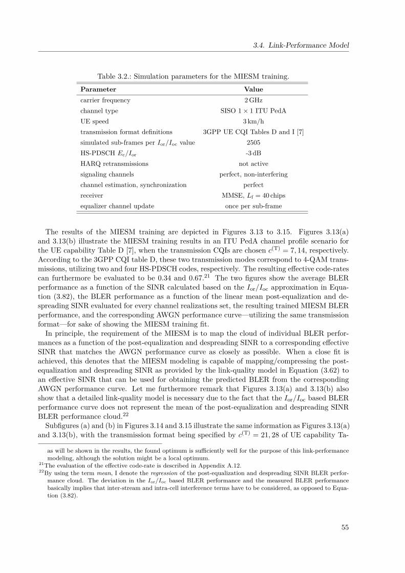
3.4. Link-Performance Model
Table 3.2.: Simulation parameters for the MIESM training.Parameter Valuecarrier frequency 2 GHzchannel type SISO 1× 1 ITU PedAUE speed 3 km/htransmission format definitions 3GPP UE CQI Tables D and I [7]simulated sub-frames per Ior/Ioc value 2505HS-PDSCH Ec/Ior -3 dBHARQ retransmissions not activesignaling channels perfect, non-interferingchannel estimation, synchronization perfectreceiver MMSE, Lf = 40 chipsequalizer channel update once per sub-frame
The results of the MIESM training are depicted in Figures 3.13 to 3.15. Figures 3.13(a)and 3.13(b) illustrate the MIESM training results in an ITU PedA channel profile scenario forthe UE capability Table D [7], when the transmission CQIs are chosen c(T) = 7, 14, respectively.According to the 3GPP CQI table D, these two transmission modes correspond to 4-QAM trans-missions, utilizing two and four HS-PDSCH codes, respectively. The resulting effective code-ratescan furthermore be evaluated to be 0.34 and 0.67.21 The two figures show the average BLERperformance as a function of the SINR calculated based on the Ior/Ioc approximation in Equa-tion (3.82), the BLER performance as a function of the linear mean post-equalization and de-spreading SINR evaluated for every channel realizations set, the resulting trained MIESM BLERperformance, and the corresponding AWGN performance curve—utilizing the same transmissionformat—for sake of showing the MIESM training fit.
In principle, the requirement of the MIESM is to map the cloud of individual BLER perfor-mances as a function of the post-equalization and despreading SINR to a corresponding effectiveSINR that matches the AWGN performance curve as closely as possible. When a close fit isachieved, this denotes that the MIESM modeling is capable of mapping/compressing the post-equalization and despreading SINR as provided by the link-quality model in Equation (3.62) toan effective SINR that can be used for obtaining the predicted BLER from the correspondingAWGN performance curve. Let me furthermore remark that Figures 3.13(a) and 3.13(b) alsoshow that a detailed link-quality model is necessary due to the fact that the Ior/Ioc based BLERperformance curve does not represent the mean of the post-equalization and despreading SINRBLER performance cloud.22
Subfigures (a) and (b) in Figures 3.14 and 3.15 illustrate the same information as Figures 3.13(a)and 3.13(b), with the transmission format being specified by c(T) = 21, 28 of UE capability Ta-
as will be shown in the results, the found optimum is sufficiently well for the purpose of this link-performancemodeling, although the solution might be a local optimum.
21The evaluation of the effective code-rate is described in Appendix A.12.22By using the term mean, I denote the regression of the post-equalization and despreading SINR BLER perfor-
mance cloud. The deviation in the Ior/Ioc based BLER performance and the measured BLER performancebasically implies that inter-stream and intra-cell interference terms have to be considered, as opposed to Equa-tion (3.82).
55
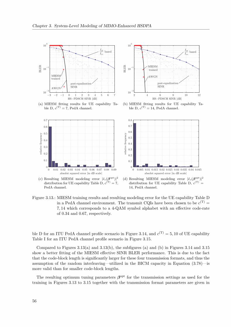
Chapter 3. System-Level Modeling of MIMO-Enhanced HSDPA
−3 −2 −1 0 1 2 3 4 5 6 710
−2
10−1
100
HS−PDSCH SINR [dB]
BLE
R
AWGN
based
MIESMtrained
post-equalizationSINR
(a) MIESM fitting results for UE capability Ta-ble D, c(T) = 7, PedA channel.
2 4 6 8 10 1210
−2
10−1
100
HS−PDSCH SINR [dB]
BLE
R
AWGN
based
MIESMtrained
post-equalizationSINR
(b) MIESM fitting results for UE capability Ta-ble D, c(T) = 14, PedA channel.
0 0.01 0.02 0.03 0.04 0.05 0.06 0.07 0.08 0.090
0.1
0.2
0.3
0.4
0.5
0.6
0.7
absolut squared error [in dB scale]
rela
tive
fre
quen
cy
(c) Resulting MIESM modeling error |ec(βopt)|2distribution for UE capability Table D, c(T) = 7,PedA channel.
0 0.005 0.01 0.015 0.02 0.025 0.03 0.035 0.04 0.0450
0.1
0.2
0.3
0.4
0.5
0.6
0.7
0.8
absolut squared error [in dB scale]
rela
tive
fre
quen
cy
(d) Resulting MIESM modeling error |ec(βopt)|2distribution for UE capability Table D, c(T) =14, PedA channel.
Figure 3.13.: MIESM training results and resulting modeling error for the UE capability Table Din a PedA channel environment. The transmit CQIs have been chosen to be c(T) =7, 14 which corresponds to a 4-QAM symbol alphabet with an effective code-rateof 0.34 and 0.67, respectively.
ble D for an ITU PedA channel profile scenario in Figure 3.14, and c(T) = 5, 10 of UE capabilityTable I for an ITU PedA channel profile scenario in Figure 3.15.
Compared to Figures 3.13(a) and 3.13(b), the subfigures (a) and (b) in Figures 3.14 and 3.15show a better fitting of the MIESM effective SINR BLER performance. This is due to the factthat the code-block length is significantly larger for these four transmission formats, and thus theassumption of the random interleaving—utilized in the BICM capacity in Equation (3.78)—ismore valid than for smaller code-block lengths.
The resulting optimum tuning parameters βopt for the transmission settings as used for thetraining in Figures 3.13 to 3.15 together with the transmission format parameters are given in
56
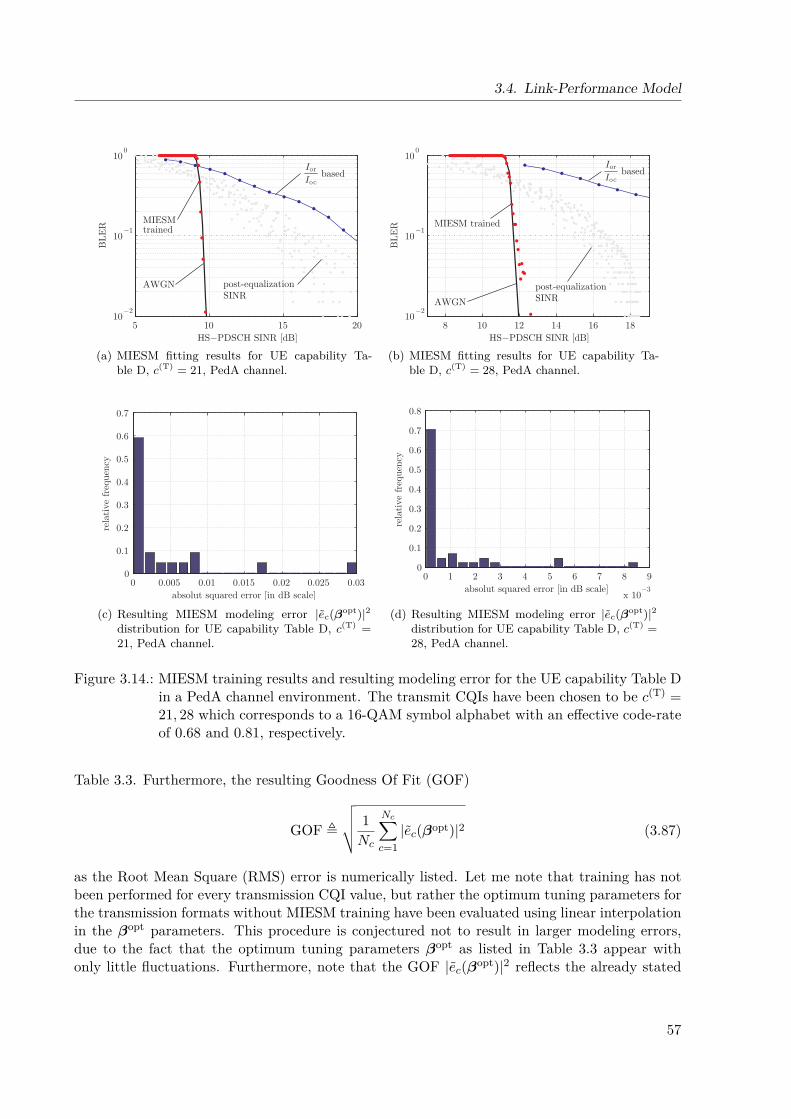
3.4. Link-Performance Model
5 10 15 2010
−2
10−1
100
HS−PDSCH SINR [dB]
BLE
R
AWGN
based
MIESMtrained
post-equalizationSINR
(a) MIESM fitting results for UE capability Ta-ble D, c(T) = 21, PedA channel.
8 10 12 14 16 1810
−2
10−1
100
HS−PDSCH SINR [dB]
BLE
R
AWGN
based
MIESM trained
post-equalizationSINR
(b) MIESM fitting results for UE capability Ta-ble D, c(T) = 28, PedA channel.
0 0.005 0.01 0.015 0.02 0.025 0.030
0.1
0.2
0.3
0.4
0.5
0.6
0.7
absolut squared error [in dB scale]
rela
tive
fre
quen
cy
(c) Resulting MIESM modeling error |ec(βopt)|2distribution for UE capability Table D, c(T) =21, PedA channel.
0 1 2 3 4 5 6 7 8 9
x 10−3
0
0.1
0.2
0.3
0.4
0.5
0.6
0.7
0.8
absolut squared error [in dB scale]
rela
tive
fre
quen
cy
(d) Resulting MIESM modeling error |ec(βopt)|2distribution for UE capability Table D, c(T) =28, PedA channel.
Figure 3.14.: MIESM training results and resulting modeling error for the UE capability Table Din a PedA channel environment. The transmit CQIs have been chosen to be c(T) =21, 28 which corresponds to a 16-QAM symbol alphabet with an effective code-rateof 0.68 and 0.81, respectively.
Table 3.3. Furthermore, the resulting Goodness Of Fit (GOF)
GOF ,
√√√√ 1Nc
Nc∑c=1|ec(βopt)|2 (3.87)
as the Root Mean Square (RMS) error is numerically listed. Let me note that training has notbeen performed for every transmission CQI value, but rather the optimum tuning parameters forthe transmission formats without MIESM training have been evaluated using linear interpolationin the βopt parameters. This procedure is conjectured not to result in larger modeling errors,due to the fact that the optimum tuning parameters βopt as listed in Table 3.3 appear withonly little fluctuations. Furthermore, note that the GOF |ec(βopt)|2 reflects the already stated
57
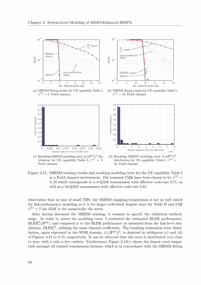
Chapter 3. System-Level Modeling of MIMO-Enhanced HSDPA
0 2 4 6 8 10 12 1410
−2
10−1
100
HS−PDSCH SINR [dB]
BLE
R
AWGN
based
MIESMtrained
post-equalizationSINR
(a) MIESM fitting results for UE capability Table I,c(T) = 5, PedA channel.
6 8 10 12 14 16 1810
−2
10−1
100
HS−PDSCH SINR [dB]
BLE
R
AWGN
based
MIESM trained
post-equalizationSINR
(b) MIESM fitting results for UE capability Table I,c(T) = 10, PedA channel.
0 0.005 0.01 0.015 0.02 0.025 0.03 0.0350
0.1
0.2
0.3
0.4
0.5
0.6
0.7
0.8
0.9
absolut squared error [in dB scale]
rela
tive
fre
quen
cy
(c) Resulting MIESM modeling error |ec(βopt)|2 dis-tribution for UE capability Table I, c(T) = 5,PedA channel.
0 1 2 3 4 5 6 7 8
x 10−3
0
0.1
0.2
0.3
0.4
0.5
0.6
0.7
0.8
absolut squared error [in dB scale]
rela
tive
fre
quen
cy
(d) Resulting MIESM modeling error |ec(βopt)|2distribution for UE capability Table I, c(T) =10, PedA channel.
Figure 3.15.: MIESM training results and resulting modeling error for the UE capability Table Iin a PedA channel environment. The transmit CQIs have been chosen to be c(T) =5, 10 which corresponds to a 4-QAM transmission with effective code-rate 0.71, aswell as a 16-QAM transmission with effective code-rate 0.81.
observation that in case of small TBS, the MIESM mapping/compression is not as well suitedfor link-performance modeling as it is for larger code-block lengths since for Table D and CQIc(T) = 7 the GOF is the numerically the worst.
After having discussed the MIESM training, it remains to specify the validation method-ology. In order to assess the modeling error, I evaluated the estimated BLER performance,BLERE
c (βopt), and compared it to the BLER performance as measured from the link-level sim-ulations, BLERM
c , utilizing the same channel coefficients. The resulting estimation error distri-bution, again expressed in the SINR domain, |ec(βopt)|2, is depicted in subfigures (c) and (d)of Figures 3.13 to 3.15, respectively. It can be observed that the error is distributed very closeto zero, with a only a few outliers. Furthermore, Figure 3.13(c) shows the largest error magni-tude amongst all trained transmission formats, which is in concordance with the MIESM fitting
58
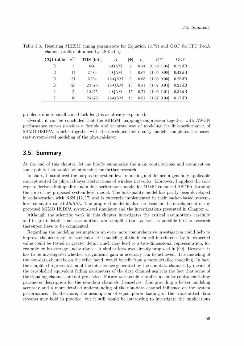
3.5. Summary
Table 3.3.: Resulting MIESM tuning parameters for Equation (3.79) and GOF for ITU PedAchannel profiles obtained by LS fitting.CQI table c(T) TBS [bits] A |Φ| rc βopt GOF
D 7 650 4-QAM 2 0.34 [0.98 1.05] 0.72 dBD 14 2 583 4-QAM 4 0.67 [1.05 0.98] 0.42 dBD 21 6 554 16-QAM 5 0.68 [1.06 0.96] 0.28 dBD 28 23 370 16-QAM 15 0.81 [1.07 0.94] 0.21 dBI 5 10 255 4-QAM 15 0.71 [1.06 1.01] 0.31 dBI 10 23 370 16-QAM 15 0.81 [1.07 0.94] 0.17 dB
problems due to small code-block lengths as already explained.Overall, it can be concluded that the MIESM mapping/compression together with AWGN
performance curves provides a flexible and accurate way of modeling the link-performance ofMIMO HSDPA, which—together with the developed link-quality model—completes the neces-sary system-level modeling of the physical-layer.
3.5. Summary
At the end of this chapter, let me briefly summarize the main contributions and comment onsome points that would be interesting for further research.
In short, I introduced the purpose of system-level modeling and defined a generally applicableconcept suited for physical-layer abstractions of wireless networks. Moreover, I applied the con-cept to derive a link-quality and a link-performance model for MIMO enhanced HSDPA, formingthe core of my proposed system-level model. The link-quality model has partly been developedin collaboration with NSN [12, 17] and is currently implemented in their packet-based system-level simulator called MoRSE. The proposed model is also the basis for the development of myproposed MIMO HSDPA system-level simulator and the investigations presented in Chapter 4.
Although the scientific work in this chapter investigates the critical assumptions carefullyand in great detail, some assumptions and simplifications as well as possible further researchthereupon have to be commented.
Regarding the modeling assumptions an even more comprehensive investigation could help toimprove the accuracy. In particular, the modeling of the intra-cell interference by its expectedvalue could be tested in greater detail which may lead to a two-dimensional representation, forexample by its average and variance. A similar idea was already proposed in [99]. However, ithas to be investigated whether a significant gain in accuracy can be achieved. The modeling ofthe non-data channels, on the other hand, would benefit from a more detailed modeling. In fact,the simplified representation of the interference generated by the non-data channels by means ofthe established equivalent fading parameters of the data channel neglects the fact that some ofthe signaling channels are not pre-coded. Future work could establish a similar equivalent fadingparameter description for the non-data channels themselves, thus providing a better modelingaccuracy and a more detailed understanding of the non-data channel influence on the systemperformance. Furthermore, the assumption of equal power loading of the transmitted datastreams may hold in practice, but it still would be interesting to investigate the implications
59
Chapter 3. System-Level Modeling of MIMO-Enhanced HSDPA
of non-homogeneous power loading to optimize the D-TxAA operation of HSDPA. This wouldcorrespond to the water-filling idea well known from information theory [51].
Also the link-performance model still offers room for further improvement. The influence ofthe UE speed—and its implications on the channel coherence time—would be worth investigatingin greater detail. HSDPA was originally targeted for lower speeds but it may nevertheless be ofinterest to assess the system-level implications of UEs moving with higher speeds. More relatedto current practical implications is that the influence of the turbo encoder block length is onlyexplicitly included in the link-performance model at the moment. In fact, if a more detailedmodeling of the coding blocklength would be derived, the better understanding of this effectcould help to optimize the link-adaptation of HSDPA. Note also that the coding blocklengthas an influencing factor is currently not directly reflected in the concept of the presented link-performance model. An improved version of the concept thus would also appear to be moregeneral and could help to develop an analytical representation of the link-performance model.Such a representation would be required for analytical network optimization approaches.
Finally, let me point out that future mobile terminals may rely on non-linear receiver structuresto achieve higher data throughput. Due to the structure of the proposed link-quality and link-performance model, however, only linear receive filters can be accurately modeled. This approachis perfectly suited for the MMSE receive filter as recommended for HSDPA by 3GPP [7], butupcoming developments suggest the usage of SIC or even ML like receiver structures. Thesewould require a significant redesign of both models in a number of places. In this context, itmight as well be of interest to investigate the modeling of the inter-cell interference in greaterdetail to allow for the system-level representation of inter-cell interference aware receivers.
Given the characteristics of future generation mobile networks as well as the importanceof system-level investigations for network operators and network equipment vendors, accuratesystem-level modeling will remain an crucial research topic.
60
Chapter 4.
System-Level-Simulation-Based Optimization ofMIMO-Enhanced HSDPA
Without change there is noinnovation, creativity, or incentivefor improvement. Those who initiatechange will have a betteropportunity to manage the changethat is inevitable.
(William Pollard)
Link-quality and link-performance models serve as the core of any system-level investigation,however for practical performance assessments and optimizations, a system-level simulator
covering mostly all procedures, algorithms, and deployment characteristics as illustrated in Fig-ure 3.2 has to be developed. This chapter thus is devoted to develop a suitable system-levelsimulator incorporating the link-quality and the link-performance model of Chapter 3 and itsapplication to conduct HSDPA network performance investigations and optimizations.
Despite the assumptions and limitations of the link-quality and link-performance modeling,also the basic design principles of the system-level simulator confine its applicability for networkalgorithm testing, equipment development, network planing, or even performance testing. Ma-jor manufacturers of mobile communication equipment, like NSN, Motorola or Ericsson operatetheir own proprietary system-level simulators to derive important results for the standardizationprocess in the 3GPP and to conduct algorithm optimizations. However, these simulators arenot publicly available and the commercial ones focus more on network planing, like for exam-ple [106]. Some open-source solutions for simulating HSDPA networks are based on the networksimulator NS-2 [107], for example [108], however these simulators focus more on the core-networkimplications—thus the IP domain—than the physical-layer and MAC-hs issues.
For the investigations that were of interest in the context of this thesis, a system-level simulatorcapable of representing the MAC for HSDPA and some RRC algorithms is more appropriate.A similar simulation approach has been taken in [109], however, the physical-layer was notmodeled by a detailed system-level model. Furthermore, the commercial simulator [110] utilizesa comparable concept, however, it does not provide the required flexibility.
Given the simulator requirements for the planned investigations and the lack of suitable open-source MIMO HSDPA system-level simulators meeting those requirements, a new Release 7HSDPA system-level simulator based on the link-quality and link-performance models of Chap-ter 3 had to be developed.1 The design focus is put onto the MAC-hs and RRC routines, thuscapturing the wireless access part of the HSDPA network including parts of the RLC layer.
1Note that the simulator utilized for the investigations in Appendix B.1 being able to represent Release 5 HSDPAis in its basic concept comparable to the simulator structure proposed in this chapter.
61
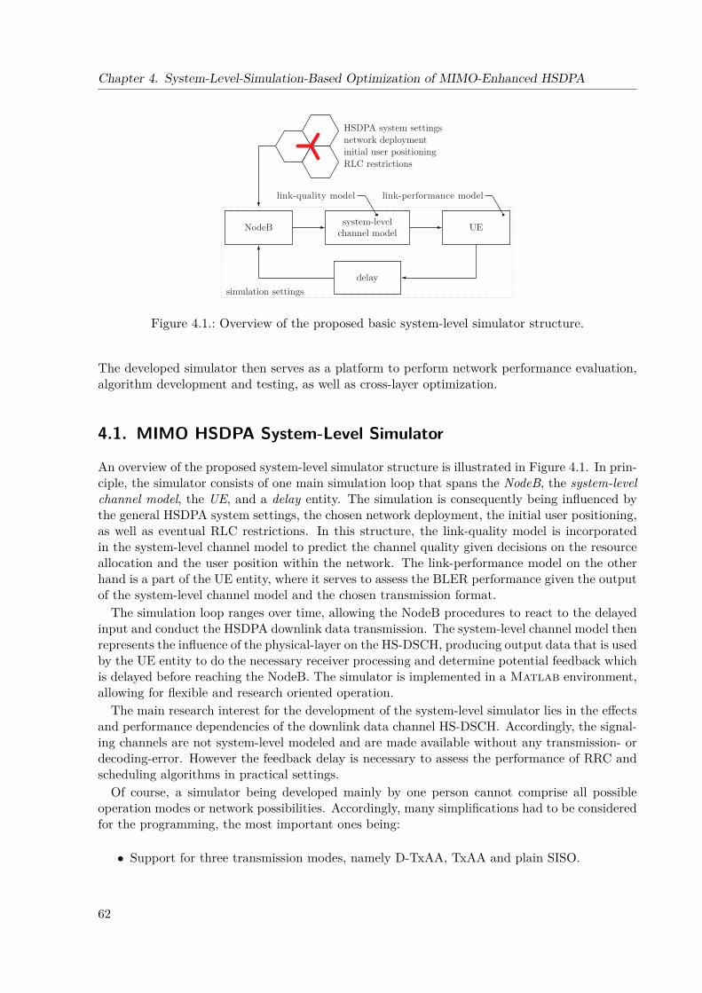
Chapter 4. System-Level-Simulation-Based Optimization of MIMO-Enhanced HSDPA
NodeB system-levelchannel model
UE
delay
network deploymentinitial user positioningRLC restrictions
HSDPA system settings
simulation settings
link-quality model link-performance model
Figure 4.1.: Overview of the proposed basic system-level simulator structure.
The developed simulator then serves as a platform to perform network performance evaluation,algorithm development and testing, as well as cross-layer optimization.
4.1. MIMO HSDPA System-Level Simulator
An overview of the proposed system-level simulator structure is illustrated in Figure 4.1. In prin-ciple, the simulator consists of one main simulation loop that spans the NodeB, the system-levelchannel model, the UE, and a delay entity. The simulation is consequently being influenced bythe general HSDPA system settings, the chosen network deployment, the initial user positioning,as well as eventual RLC restrictions. In this structure, the link-quality model is incorporatedin the system-level channel model to predict the channel quality given decisions on the resourceallocation and the user position within the network. The link-performance model on the otherhand is a part of the UE entity, where it serves to assess the BLER performance given the outputof the system-level channel model and the chosen transmission format.
The simulation loop ranges over time, allowing the NodeB procedures to react to the delayedinput and conduct the HSDPA downlink data transmission. The system-level channel model thenrepresents the influence of the physical-layer on the HS-DSCH, producing output data that is usedby the UE entity to do the necessary receiver processing and determine potential feedback whichis delayed before reaching the NodeB. The simulator is implemented in a Matlab environment,allowing for flexible and research oriented operation.
The main research interest for the development of the system-level simulator lies in the effectsand performance dependencies of the downlink data channel HS-DSCH. Accordingly, the signal-ing channels are not system-level modeled and are made available without any transmission- ordecoding-error. However the feedback delay is necessary to assess the performance of RRC andscheduling algorithms in practical settings.
Of course, a simulator being developed mainly by one person cannot comprise all possibleoperation modes or network possibilities. Accordingly, many simplifications had to be consideredfor the programming, the most important ones being:
• Support for three transmission modes, namely D-TxAA, TxAA and plain SISO.
62

4.1. MIMO HSDPA System-Level Simulator
• The supported receiver types are MMSE equalizer and Rake receiver.2
• The maximum number of supported streams equals two, NS = 2.3
• The supported UE capability classes are 16 and 18 which are the UE capability classeswith the highest supported throughput. The according CQI tables in [7] are the Tables C,D, H, and I.• The supported modulation alphabets are 4-QAM and 16-QAM.• No handover support between sectors.• Users are only simulated in the target sector of the center cell, which means that most of
the network algorithms are only active in the target sector, where full UE data is avail-able. Given the fact that no handover investigations are supported, the simulation of theneighboring cells as pure interference sources is sufficient.• No support for inter-cell coordination which prevents the investigation of inter-cell inter-
ference management.• Restriction of the utilizable TFCI set to the set of CQI corresponding TFC, and• a full buffer assumption.
Most of these simplifications are necessary to make the simulator easier to implement, howeverthey can be relaxed to the expense of additional significant programming work. Although re-stricting the scope of research questions that can be answered with the simulator, the featuresof it are more than sufficient for the questions examined in this thesis.
4.1.1. Detailed Simulator Structure
Let me go into more detail on the procedural implementation of the main simulator parts.Figure 4.2 shows the basic procedures of the NodeB-entity implementation in the system-levelsimulator. The delayed UE output—containing at least the ACK/NACK and CQI feedbackinformation—is first buffered. This is necessary, if one of the following algorithms wants tohave access to the history of the incoming feedback information to allow for example for theprediction of channel states or achievable data-rates. After this initial stage, the scheduler isresponsible for determining which user will obtain the physical downlink resources.4 After thescheduler decision is taken, the NodeB may conduct the so-called stream decision, indicating thealgorithm potentially deciding upon the number of spatial streams that will be utilized in thedownlink transmission. This basically corresponds to the decision between D-TxAA and TxAAtransmission modes. Furthermore, let me note that [7] allows the UE to feedback whether oneor two streams are requested. Nevertheless it may be sometimes beneficial to overrule the UErequest, as will be elaborated in Section 4.3.
Depending on the scheduler and stream decisions, the physical channel utilization in form ofthe link-adaptation TFC will be determined. The restriction of the set of TFCI to the set of
2Recall that Interference Cancellation (IC) receiver structures are not modeled by the system-level model devel-oped in Chapter 3.
3Note that this is an implementation restriction, the system-level model of Chapter 3 would allow for the simu-lation of higher order spatial multiplexing schemes.
4Or which users will obtain which amount of physical downlink resources in the multi-user scheduling case.Physical downlink resources in this context mainly denotes the number of HS-PDSCHs available for eachscheduled user, respectively.
63
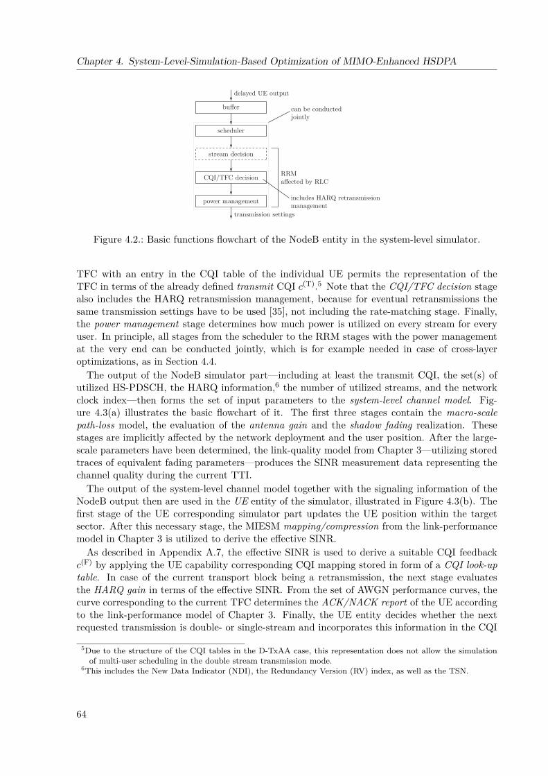
Chapter 4. System-Level-Simulation-Based Optimization of MIMO-Enhanced HSDPA
buffer
delayed UE output
scheduler
stream decision
CQI/TFC decision
power management
RRMaffected by RLC
can be conductedjointly
includes HARQ retransmissionmanagement
transmission settings
Figure 4.2.: Basic functions flowchart of the NodeB entity in the system-level simulator.
TFC with an entry in the CQI table of the individual UE permits the representation of theTFC in terms of the already defined transmit CQI c(T).5 Note that the CQI/TFC decision stagealso includes the HARQ retransmission management, because for eventual retransmissions thesame transmission settings have to be used [35], not including the rate-matching stage. Finally,the power management stage determines how much power is utilized on every stream for everyuser. In principle, all stages from the scheduler to the RRM stages with the power managementat the very end can be conducted jointly, which is for example needed in case of cross-layeroptimizations, as in Section 4.4.
The output of the NodeB simulator part—including at least the transmit CQI, the set(s) ofutilized HS-PDSCH, the HARQ information,6 the number of utilized streams, and the networkclock index—then forms the set of input parameters to the system-level channel model. Fig-ure 4.3(a) illustrates the basic flowchart of it. The first three stages contain the macro-scalepath-loss model, the evaluation of the antenna gain and the shadow fading realization. Thesestages are implicitly affected by the network deployment and the user position. After the large-scale parameters have been determined, the link-quality model from Chapter 3—utilizing storedtraces of equivalent fading parameters—produces the SINR measurement data representing thechannel quality during the current TTI.
The output of the system-level channel model together with the signaling information of theNodeB output then are used in the UE entity of the simulator, illustrated in Figure 4.3(b). Thefirst stage of the UE corresponding simulator part updates the UE position within the targetsector. After this necessary stage, the MIESM mapping/compression from the link-performancemodel in Chapter 3 is utilized to derive the effective SINR.
As described in Appendix A.7, the effective SINR is used to derive a suitable CQI feedbackc(F) by applying the UE capability corresponding CQI mapping stored in form of a CQI look-uptable. In case of the current transport block being a retransmission, the next stage evaluatesthe HARQ gain in terms of the effective SINR. From the set of AWGN performance curves, thecurve corresponding to the current TFC determines the ACK/NACK report of the UE accordingto the link-performance model of Chapter 3. Finally, the UE entity decides whether the nextrequested transmission is double- or single-stream and incorporates this information in the CQI
5Due to the structure of the CQI tables in the D-TxAA case, this representation does not allow the simulationof multi-user scheduling in the double stream transmission mode.
6This includes the New Data Indicator (NDI), the Redundancy Version (RV) index, as well as the TSN.
64
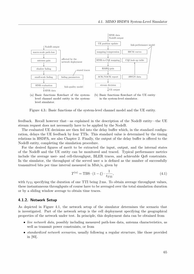
4.1. MIMO HSDPA System-Level Simulator
macro-scale path-loss
antenna gain
shadow fading
small-scale fading
SINR evaluation
NodeB output
SINR data
affected by thenetwork deployment
link-quality model
fading parameters
stored traces
(a) Basic functions flowchart of the system-level channel model entity in the system-level simulator.
UE position update
SINR-to-CQI mapping
HARQ gain
ACK/NACK report
stream decision
mapping/compression
SINR dataNodeB output
AWGN data
CQI look-up table
BICM curves
UE output
link-performance model
(b) Basic functions flowchart of the UE entityin the system-level simulator.
Figure 4.3.: Basic functions of the system-level channel model and the UE entity.
feedback. Recall however that—as explained in the description of the NodeB entity—the UEstream request does not necessarily have to be applied by the NodeB.
The evaluated UE decisions are then fed into the delay buffer which, in the standard configu-ration, delays the UE feedback by four TTIs. This standard value is determined by the timingrelations in HSDPA, see also Chapter 2. Finally, the output of the delay buffer is offered to theNodeB entity, completing the simulation procedure.
For the desired figures of merit to be extracted the input, output, and the internal statesof the NodeB and the UE entity can be monitored and traced. Typical performance metricsinclude the average user- and cell-throughput, BLER traces, and achievable QoS constraints.In the simulator, the throughput of the served user u is defined as the number of successfullytransmitted bits per time interval measured in Mbit/s, given by
T (u) = TBS · (1− ξ) · 1tTTI
, (4.1)
with tTTI specifying the duration of one TTI being 2 ms. To obtain average throughput values,these instantaneous throughputs of course have to be averaged over the total simulation durationor by a sliding window average to obtain time traces.
4.1.2. Network SetupAs depicted in Figure 4.1, the network setup of the simulator determines the scenario thatis investigated. Part of the network setup is the cell deployment specifying the geographicalproperties of the network under test. In principle, this deployment data can be obtained from
• live network data, possibly including measured path-loss data, antenna characteristics, aswell as transmit power constraints, or from• standardized network scenarios, usually following a regular structure, like those provided
in [93].
65
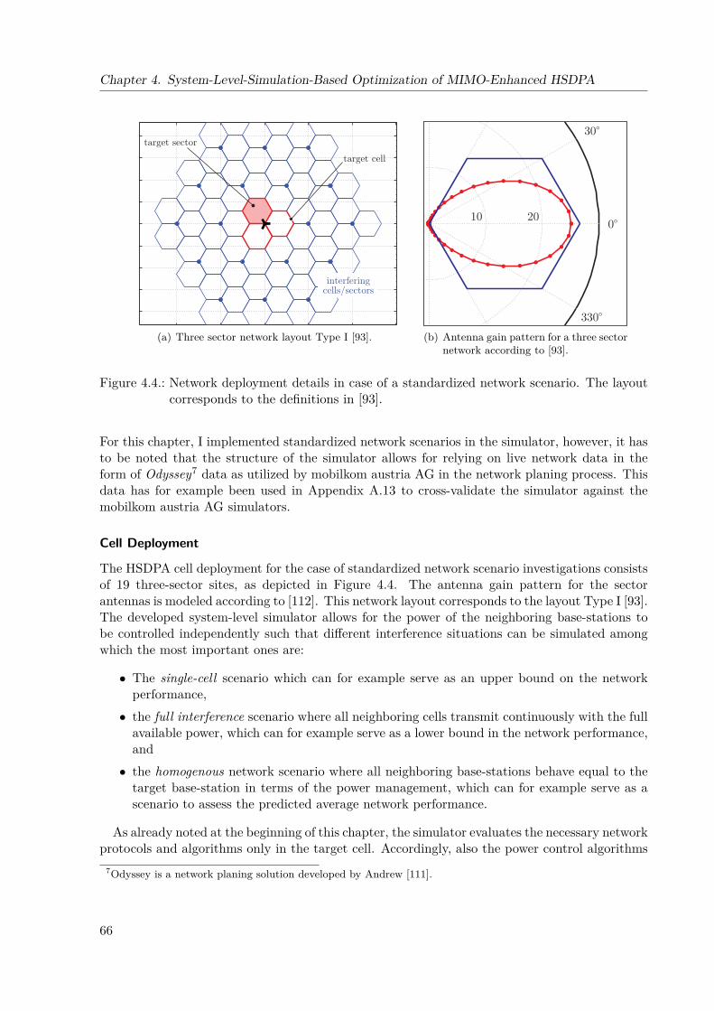
Chapter 4. System-Level-Simulation-Based Optimization of MIMO-Enhanced HSDPA
interferingcells/sectors
target cell
target sector
(a) Three sector network layout Type I [93].
30°
330°
0°10 20
(b) Antenna gain pattern for a three sectornetwork according to [93].
Figure 4.4.: Network deployment details in case of a standardized network scenario. The layoutcorresponds to the definitions in [93].
For this chapter, I implemented standardized network scenarios in the simulator, however, it hasto be noted that the structure of the simulator allows for relying on live network data in theform of Odyssey7 data as utilized by mobilkom austria AG in the network planing process. Thisdata has for example been used in Appendix A.13 to cross-validate the simulator against themobilkom austria AG simulators.
Cell Deployment
The HSDPA cell deployment for the case of standardized network scenario investigations consistsof 19 three-sector sites, as depicted in Figure 4.4. The antenna gain pattern for the sectorantennas is modeled according to [112]. This network layout corresponds to the layout Type I [93].The developed system-level simulator allows for the power of the neighboring base-stations tobe controlled independently such that different interference situations can be simulated amongwhich the most important ones are:
• The single-cell scenario which can for example serve as an upper bound on the networkperformance,• the full interference scenario where all neighboring cells transmit continuously with the full
available power, which can for example serve as a lower bound in the network performance,and• the homogenous network scenario where all neighboring base-stations behave equal to the
target base-station in terms of the power management, which can for example serve as ascenario to assess the predicted average network performance.
As already noted at the beginning of this chapter, the simulator evaluates the necessary networkprotocols and algorithms only in the target cell. Accordingly, also the power control algorithms
7Odyssey is a network planing solution developed by Andrew [111].
66

4.1. MIMO HSDPA System-Level Simulator
0 0.1 0.2 0.3 0.4 0.570
80
90
100
110
120
130
140
distance NodeB-UE [km]
mac
ro−
scal
e pa
th−
loss
[dB
]
urban micro
urban macro
(a) Macro-scale path-loss for urban micro and urbanmacro scenarios according to [112].
distance NodeB-UE [m]
dist
ance
Nod
eB-U
E [m
]
−500 0 500 1000 1500−1000
−800
−600
−400
−200
0
200
400
600
800
1000
−20
−15
−10
−5
0
5
10
(b) Pre-equalization SINR Ior/Ioc in dB in thetarget sector according to the urban micropath-loss model.
Figure 4.5.: Macro-scale path-loss model results in terms of the path-loss and the resulting aver-age receive power distribution.
are only evaluated in detail for the target cell, which limits the interference scenarios to be as-sessed. Nevertheless, situations in which the neighboring base-stations have different maximumoutput powers available can be simulated. Situations of this kind are of interest for mobile net-work operators to assess for example the implications of new power-amplifiers to support higheroutput power values onto the interference situation and thus the target base-station performance.
Propagation Modeling
When a standardized network scenario is considered, the propagation modeling is of importance.Propagation models for system-level simulations should be chosen to adequately represent theenvironment of interest. In [112] different propagation models for urban and suburban environ-ments have been defined. I implemented two of the defined models in the simulator, the EuropeanCOoperation in the field of Scientific and Technical research (COST) 231 extended Hata modeland the COST 231 Walfish-Ikegami model. The COST 231 extended Hata model is applied incase of suburban macro- and urban macro-cell deployments.8 The COST 231 Walfish-Ikegamimodel, on the other hand, is applied in case of urban micro-cell layouts.9 In the following, let medenote the resulting macro-scale path-loss between user u and base-station b by λ(u,b)
m . Figure 4.5depicts the path-loss in dB as predicted by the urban micro and the urban macro model withthe settings defined as specified for MIMO HSDPA evaluations [93]. It can be observed that theminimum path-loss is limited to the free-space path-loss in both cases.
To model sectored networks, antennas with a corresponding gain pattern have to be considered,see Figure 4.4. Let me denote the antenna gain as a function of the azimuth between base-stationand user by gant(θ(u,b)). Figure 4.5 illustrates the resulting pre-equalization SINR Ior/Ioc when
8The extended Hata model is restricted to a carrier frequency between 1.5 GHz and 2.0 GHz, base-station heightsbetween 30 m and 200 m, mobile station heights between 1 m and 10 m, and an inter-NodeB distance between1 km and 20 km.
9The Walfish-Ikegami model is restricted to a carrier frequency between 800 MHz and 2 GHz, a height of thebase-station between 4 m and 50 m, and a height of the mobile station between 1 m and 3 m.
67
Chapter 4. System-Level-Simulation-Based Optimization of MIMO-Enhanced HSDPA
the sector antenna of Figure 4.4 [112] is taken into account and a 19 base-station network withhomogenous maximum output power of 43 dBm is assumed.
To account for shadowing effects in the cell area, shadow fading has to be generated for eachuser-base-station link. As a result of the relief of the terrain in the cell, the shadow fading has tobe correlated in the area of the UE motion as well as between links from different base-stations.10
For these correlation effects, either correlated shadow fading maps for the cell area or correlatedtime traces can be generated. Time traces are possible due to the fact that the UEs are movingand thus are observing a shadow fading that is changing over time. Note that shadow fadingmaps with correct statistical properties have been in research for quite some time [113,114], butthey are generally quite difficult to generate and require large amounts of memory.
Accordingly, I decided to employ time-correlated shadow-fading traces in the system-levelsimulator. The spatial correlation of the shadow-fading is translated into a time-correlation bythe model of [115]. This model generates the samples by filtering a log-normal random processa(u,b), following the pdf
fa(a) , 1a σ√
2πexp
[−(ln a− µ)2
2σ2
], a > 0, (4.2)
where µ and σ are the mean and standard deviation of the natural logarithm of a, which isnormally distributed, that is ln a ∝ N
(µ, σ2). The utilized filter fshadow is of first order with one
pole that guarantees that the resulting autocorrelation Ra(u,b) is given by
a(u,b) = a(u,b) ∗ fshadow → Ra(u,b) [i] = σ2%vTs|i|1D , (4.3)
with % describing the spatial correlation coefficient at correlation distance D, and v being theUE speed. The inter-site correlation is modeled according to [93], such that the resulting shadowfading can be evaluated as
λ(u,b)s =
√1− ζa(u,b) +
√ζε(u), (4.4)
with ζ denoting the inter-site correlation coefficient and ε(u) specifying a user-specific randomoffset value drawn from a zero-mean Gaussian random process.
Finally, the overall path-loss L(u,b) combining all macro- and large-scale effects in the cell—asutilized in Equation (3.62)—is given by
L(u,b) = λ(u,b)m · gant
(θ(u,b)
)· λ(u,b)
s . (4.5)
To establish the connection to Equation (3.62) let me note that for sake of notational simplicitythe user index u had been omitted, which makes L(b) = L(u,b) in this context.
User Mobility
For a realistic performance evaluation, the simulated UEs in the target cell have to move. Ac-cordingly, I implemented a random movement mobility scheme. At the beginning of a simulationa random position in the target sector according to a uniform probability distribution over thesector area is assigned to each user. Additionally, every user is assigned a random walking direc-tion with uniform distribution over the interval [0, 2π). Since the simulator does not allow forthe simulation of handover scenarios, when a user leaves the target cell, he becomes de-attachedfrom it and a new user is generated according to the same procedure. This keeps the number ofsimulated users constant.10This means the target sector link and the interfering base-station links.
68
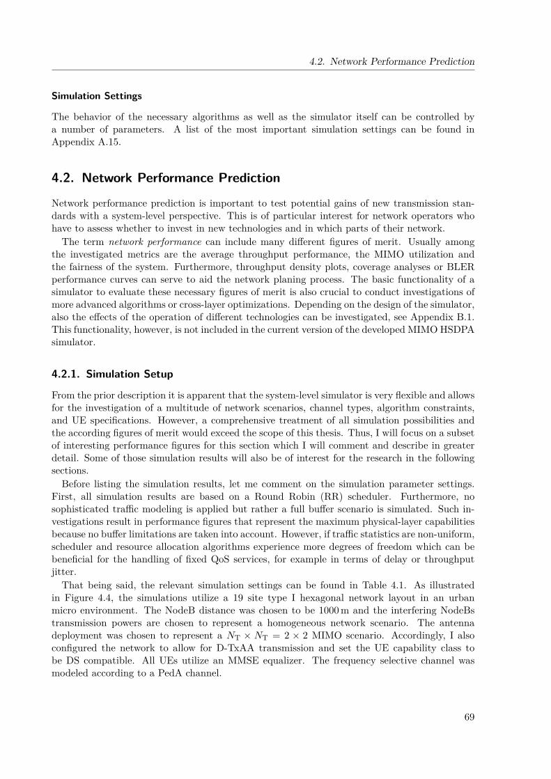
4.2. Network Performance Prediction
Simulation Settings
The behavior of the necessary algorithms as well as the simulator itself can be controlled bya number of parameters. A list of the most important simulation settings can be found inAppendix A.15.
4.2. Network Performance Prediction
Network performance prediction is important to test potential gains of new transmission stan-dards with a system-level perspective. This is of particular interest for network operators whohave to assess whether to invest in new technologies and in which parts of their network.
The term network performance can include many different figures of merit. Usually amongthe investigated metrics are the average throughput performance, the MIMO utilization andthe fairness of the system. Furthermore, throughput density plots, coverage analyses or BLERperformance curves can serve to aid the network planing process. The basic functionality of asimulator to evaluate these necessary figures of merit is also crucial to conduct investigations ofmore advanced algorithms or cross-layer optimizations. Depending on the design of the simulator,also the effects of the operation of different technologies can be investigated, see Appendix B.1.This functionality, however, is not included in the current version of the developed MIMO HSDPAsimulator.
4.2.1. Simulation Setup
From the prior description it is apparent that the system-level simulator is very flexible and allowsfor the investigation of a multitude of network scenarios, channel types, algorithm constraints,and UE specifications. However, a comprehensive treatment of all simulation possibilities andthe according figures of merit would exceed the scope of this thesis. Thus, I will focus on a subsetof interesting performance figures for this section which I will comment and describe in greaterdetail. Some of those simulation results will also be of interest for the research in the followingsections.
Before listing the simulation results, let me comment on the simulation parameter settings.First, all simulation results are based on a Round Robin (RR) scheduler. Furthermore, nosophisticated traffic modeling is applied but rather a full buffer scenario is simulated. Such in-vestigations result in performance figures that represent the maximum physical-layer capabilitiesbecause no buffer limitations are taken into account. However, if traffic statistics are non-uniform,scheduler and resource allocation algorithms experience more degrees of freedom which can bebeneficial for the handling of fixed QoS services, for example in terms of delay or throughputjitter.
That being said, the relevant simulation settings can be found in Table 4.1. As illustratedin Figure 4.4, the simulations utilize a 19 site type I hexagonal network layout in an urbanmicro environment. The NodeB distance was chosen to be 1000 m and the interfering NodeBstransmission powers are chosen to represent a homogeneous network scenario. The antennadeployment was chosen to represent a NT × NT = 2 × 2 MIMO scenario. Accordingly, I alsoconfigured the network to allow for D-TxAA transmission and set the UE capability class tobe DS compatible. All UEs utilize an MMSE equalizer. The frequency selective channel wasmodeled according to a PedA channel.
69

Chapter 4. System-Level-Simulation-Based Optimization of MIMO-Enhanced HSDPA
Table 4.1.: Simulation settings for the system-level investigations results.Parameter Valueinterference scenario homogeneous networknumber of cells 19, layout type INodeB distance 1000 mcarrier frequency 1.9 GHztotal transmit power available at NodeB 20 Wtotal CPICH power 0.8 Wpower of other channels 1.2 Wavailable HS-PDSCHs 15macro-scale path-loss model urban microantenna utilization NT ×NR = 2× 2channel type ITU PedAscheduler RRactive users in target sector 25user mobility 3 km/h, random directionUE capability class 20UE receiver type MMSE, Lf = 30 chips, τ = 15 chipsfeedback delay 4 TTIsimulation time 50 000 slots, each 2/3 ms
The feedback delay for reporting the ACK/NACK and the CQI report was set according to thetiming constraints [7] to 4 TTIs. Finally, the stream power loading is conducted in a uniform way,thus no power loading of the individual streams is performed. For the HS-DSCH transmission,all 15 possible HS-PDSCH are available which leaves no room for UMTS traffic in the cell thusthese results represent a dedicated MIMO HSDPA network.
4.2.2. Single Network Scenario Investigation
The first results that can be obtained from a system-level simulation are based on a singlenetwork realization. In general, the term network realization corresponds to a user positioningand movement realization, given the network layout and algorithm constraints.11 Althoughlimited in significance for assessing the overall network performance, these results can serve toidentify whether and how well the basic adaptation mechanisms of HSDPA work, and to obtainsome knowledge about the performance limits of the system.
In Figure 4.6 the resulting ecdfs of the corresponding throughput values and the underlyinginitial user positioning are depicted. The ecdfs of the worst and the best user throughputrepresent the performance bounds for the scheduler given the network realization. Depending onthe scheduler strategy, in particular its fairness constraints, the sector throughput statistics canbe closer to the best user throughput.11By the term algorithmic constraints I denote the utilization of the power and resource allocation schemes as
introduced.
70

4.2. Network Performance Prediction
0 5 10 15 20 250
0.1
0.2
0.3
0.4
0.5
0.6
0.7
0.8
0.9
1
sector and user throughput [Mbit/s]
ecdf
best user
worst user
sector
(a) The ecdfs of the worst user, best user and sectorthroughputs.
0 100 200 300 400 500 600
−250−200−150−100−50
050
100150200250
distance NodeB-UE [m]
dist
ance
Nod
eB-U
E [m
] best user
worst user
(b) UE positioning in the target sector.
Figure 4.6.: Single network realization SINR and throughput results.
0 5 10 15 20 25 30 350
0.02
0.04
0.06
0.08
0.1
0.12
0.14
0.16
0.18
0.2
time [s]
aver
age
AC
K/N
AC
K r
atio
Figure 4.7.: BLER results for a single network realization.
According to the system design [7] and corresponding to the SINR-to-CQI mapping fromAppendix A.7, the average ACK/NACK ratio of the cell should be close to its target value of0.1.12 To confirm this behavior in the system-level simulator, Figure 4.7 depicts the ACK/NACKratio when averaged with a sliding window filter of length 125 TTIs. It can be observed that theACK/NACK ratio fluctuates around its average of 0.11, which is close to its desired target value.
When speaking of the ACK/NACK ratio performance, it has to be noted that the responsiblelink-adaptation for stream two is much more difficult to calibrate than for stream one. Thereason is that due to the pre-coding, stream two experiences a much higher variance of its SINRand thus the link-adaptation has to be configured more conservatively. For optimum operation,the pre-coding and the stream decision should be performed in a joint way.
Figure 4.8 lists the distribution of the stream utilization and the distribution of the CQI reportsfor the SS and the DS case, respectively. It can be observed that the cell utilizes a SS transmissiontime approximately two and a half times that of the DS transmission. Furthermore, the CQIdistributions show that the dynamic range covered by the link-adaptation fits the observed12Note that the term ACK/NACK ratio is defined as [nr. of NACK/(nr. of ACK+nr. of NACK)] in this context.
71
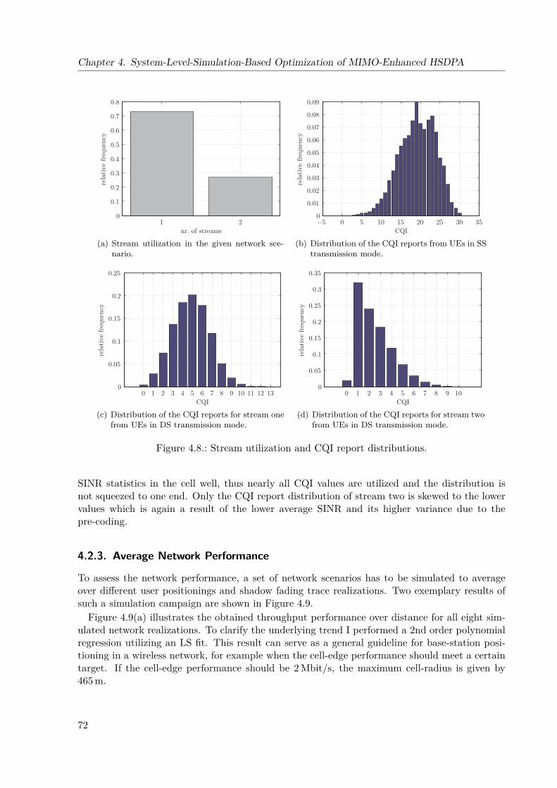
Chapter 4. System-Level-Simulation-Based Optimization of MIMO-Enhanced HSDPA
1 20
0.1
0.2
0.3
0.4
0.5
0.6
0.7
0.8
nr. of streams
rela
tive
fre
quen
cy
(a) Stream utilization in the given network sce-nario.
−5 0 5 10 15 20 25 30 350
0.01
0.02
0.03
0.04
0.05
0.06
0.07
0.08
0.09
CQI
rela
tive
fre
quen
cy
(b) Distribution of the CQI reports from UEs in SStransmission mode.
0 1 2 3 4 5 6 7 8 9 10 11 12 130
0.05
0.1
0.15
0.2
0.25
CQI
rela
tive
fre
quen
cy
(c) Distribution of the CQI reports for stream onefrom UEs in DS transmission mode.
0 1 2 3 4 5 6 7 8 9 100
0.05
0.1
0.15
0.2
0.25
0.3
0.35
CQI
rela
tive
fre
quen
cy
(d) Distribution of the CQI reports for stream twofrom UEs in DS transmission mode.
Figure 4.8.: Stream utilization and CQI report distributions.
SINR statistics in the cell well, thus nearly all CQI values are utilized and the distribution isnot squeezed to one end. Only the CQI report distribution of stream two is skewed to the lowervalues which is again a result of the lower average SINR and its higher variance due to thepre-coding.
4.2.3. Average Network Performance
To assess the network performance, a set of network scenarios has to be simulated to averageover different user positionings and shadow fading trace realizations. Two exemplary results ofsuch a simulation campaign are shown in Figure 4.9.
Figure 4.9(a) illustrates the obtained throughput performance over distance for all eight sim-ulated network realizations. To clarify the underlying trend I performed a 2nd order polynomialregression utilizing an LS fit. This result can serve as a general guideline for base-station posi-tioning in a wireless network, for example when the cell-edge performance should meet a certaintarget. If the cell-edge performance should be 2 Mbit/s, the maximum cell-radius is given by465 m.
72
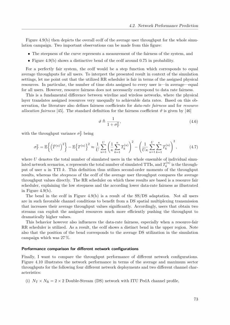
4.2. Network Performance Prediction
Figure 4.9(b) then depicts the overall ecdf of the average user throughput for the whole simu-lation campaign. Two important observations can be made from this figure:
• The steepness of the curve represents a measurement of the fairness of the system, and• Figure 4.9(b) shows a distinctive bend of the ecdf around 0.75 in probability.
For a perfectly fair system, the ecdf would be a step function which corresponds to equalaverage throughputs for all users. To interpret the presented result in context of the simulationsettings, let me point out that the utilized RR scheduler is fair in terms of the assigned physicalresources. In particular, the number of time slots assigned to every user is—in average—equalfor all users. However, resource fairness does not necessarily correspond to data rate fairness.
This is a fundamental difference between wireline and wireless networks, where the physicallayer translates assigned resources very unequally to achievable data rates. Based on this ob-servation, the literature also defines fairness coefficients for data-rate fairness and for resourceallocation fairness [45]. The standard definition for the fairness coefficient ϑ is given by [46]
ϑ ,1
1 + σ2T
, (4.6)
with the throughput variance σ2T being
σ2T = E
(T (u)
)2− E
T (u)
2≈ 1U
U∑u=1
(1κ
κ∑k=1
T(u)k
)2
−(
1Uκ
U∑u=1
κ∑k=1
T(u)k
)2
, (4.7)
where U denotes the total number of simulated users in the whole ensemble of individual simu-lated network scenarios, κ represents the total number of simulated TTIs, and T (u)
k is the through-put of user u in TTI k. This definition thus utilizes second-order moments of the throughputresults, whereas the steepness of the ecdf of the average user throughput compares the averagethroughput values directly. The RR scheduler on which these results are based is a resource fairscheduler, explaining the low steepness and the according lower data-rate fairness as illustratedin Figure 4.9(b).
The bend in the ecdf in Figure 4.9(b) is a result of the SS/DS adaptation. Not all usersare in such favorable channel conditions to benefit from a DS spatial multiplexing transmissionthat increases their average throughput values significantly. Accordingly, users that obtain twostreams can exploit the assigned resources much more efficiently pushing the throughput todramatically higher values.
This behavior however also influences the data-rate fairness, especially when a resource-fairRR scheduler is utilized. As a result, the ecdf shows a distinct bend in the upper region. Notealso that the position of the bend corresponds to the average DS utilization in the simulationcampaign which was 27 %.
Performance comparison for different network configurations
Finally, I want to compare the throughput performance of different network configurations.Figure 4.10 illustrates the network performance in terms of the average and maximum sectorthroughputs for the following four different network deployments and two different channel char-acteristics:
(i) NT ×NR = 2× 2 Double-Stream (DS) network with ITU PedA channel profile,
73
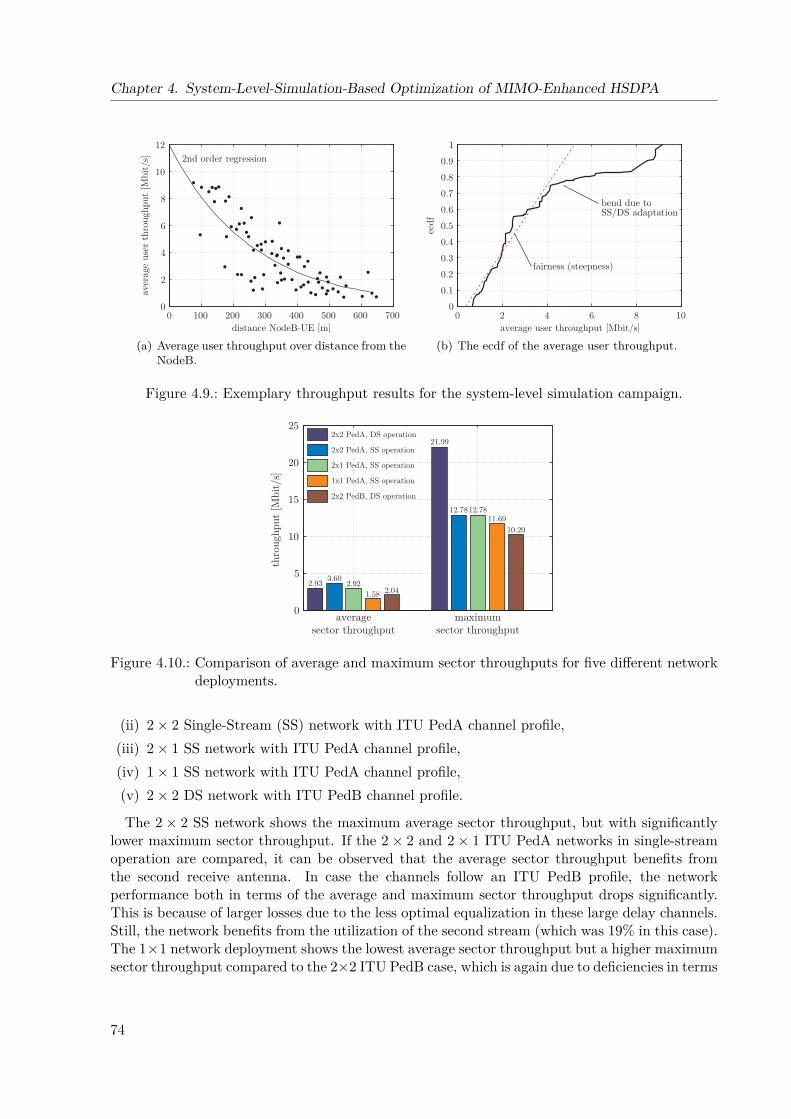
Chapter 4. System-Level-Simulation-Based Optimization of MIMO-Enhanced HSDPA
0 100 200 300 400 500 600 7000
2
4
6
8
10
12
distance NodeB-UE [m]
aver
age
user
thr
ough
put
[Mbi
t/s] 2nd order regression
(a) Average user throughput over distance from theNodeB.
0 2 4 6 8 100
0.1
0.2
0.3
0.4
0.5
0.6
0.7
0.8
0.9
1
average user throughput [Mbit/s]
ecdf
fairness (steepness)
bend due toSS/DS adaptation
(b) The ecdf of the average user throughput.
Figure 4.9.: Exemplary throughput results for the system-level simulation campaign.
averagesector throughput
maximumsector throughput
thro
ughp
ut [M
bit/
s]
0
5
10
15
20
252x2 PedA, DS operation
2x2 PedA, SS operation
2x1 PedA, SS operation
1x1 PedA, SS operation
2x2 PedB, DS operation
2.933.60
2.921.58 2.04
21.99
12.7812.7811.69
10.20
Figure 4.10.: Comparison of average and maximum sector throughputs for five different networkdeployments.
(ii) 2× 2 Single-Stream (SS) network with ITU PedA channel profile,(iii) 2× 1 SS network with ITU PedA channel profile,(iv) 1× 1 SS network with ITU PedA channel profile,(v) 2× 2 DS network with ITU PedB channel profile.
The 2 × 2 SS network shows the maximum average sector throughput, but with significantlylower maximum sector throughput. If the 2× 2 and 2× 1 ITU PedA networks in single-streamoperation are compared, it can be observed that the average sector throughput benefits fromthe second receive antenna. In case the channels follow an ITU PedB profile, the networkperformance both in terms of the average and maximum sector throughput drops significantly.This is because of larger losses due to the less optimal equalization in these large delay channels.Still, the network benefits from the utilization of the second stream (which was 19% in this case).The 1×1 network deployment shows the lowest average sector throughput but a higher maximumsector throughput compared to the 2×2 ITU PedB case, which is again due to deficiencies in terms
74
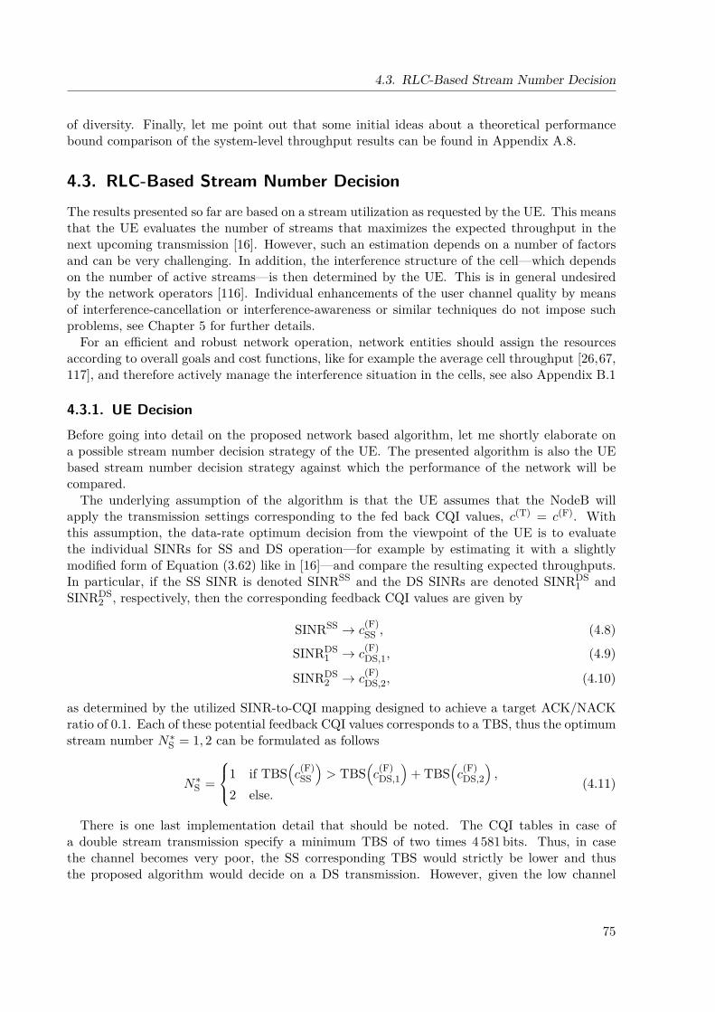
4.3. RLC-Based Stream Number Decision
of diversity. Finally, let me point out that some initial ideas about a theoretical performancebound comparison of the system-level throughput results can be found in Appendix A.8.
4.3. RLC-Based Stream Number DecisionThe results presented so far are based on a stream utilization as requested by the UE. This meansthat the UE evaluates the number of streams that maximizes the expected throughput in thenext upcoming transmission [16]. However, such an estimation depends on a number of factorsand can be very challenging. In addition, the interference structure of the cell—which dependson the number of active streams—is then determined by the UE. This is in general undesiredby the network operators [116]. Individual enhancements of the user channel quality by meansof interference-cancellation or interference-awareness or similar techniques do not impose suchproblems, see Chapter 5 for further details.
For an efficient and robust network operation, network entities should assign the resourcesaccording to overall goals and cost functions, like for example the average cell throughput [26,67,117], and therefore actively manage the interference situation in the cells, see also Appendix B.1
4.3.1. UE DecisionBefore going into detail on the proposed network based algorithm, let me shortly elaborate ona possible stream number decision strategy of the UE. The presented algorithm is also the UEbased stream number decision strategy against which the performance of the network will becompared.
The underlying assumption of the algorithm is that the UE assumes that the NodeB willapply the transmission settings corresponding to the fed back CQI values, c(T) = c(F). Withthis assumption, the data-rate optimum decision from the viewpoint of the UE is to evaluatethe individual SINRs for SS and DS operation—for example by estimating it with a slightlymodified form of Equation (3.62) like in [16]—and compare the resulting expected throughputs.In particular, if the SS SINR is denoted SINRSS and the DS SINRs are denoted SINRDS
1 andSINRDS
2 , respectively, then the corresponding feedback CQI values are given by
SINRSS → c(F)SS , (4.8)
SINRDS1 → c
(F)DS,1, (4.9)
SINRDS2 → c
(F)DS,2, (4.10)
as determined by the utilized SINR-to-CQI mapping designed to achieve a target ACK/NACKratio of 0.1. Each of these potential feedback CQI values corresponds to a TBS, thus the optimumstream number N∗S = 1, 2 can be formulated as follows
N∗S =
1 if TBS(c
(F)SS
)> TBS
(c
(F)DS,1
)+ TBS
(c
(F)DS,2
),
2 else.(4.11)
There is one last implementation detail that should be noted. The CQI tables in case ofa double stream transmission specify a minimum TBS of two times 4 581 bits. Thus, in casethe channel becomes very poor, the SS corresponding TBS would strictly be lower and thusthe proposed algorithm would decide on a DS transmission. However, given the low channel
75

Chapter 4. System-Level-Simulation-Based Optimization of MIMO-Enhanced HSDPA
quality, a successful DS transmission is very unlikely. Accordingly, there is the need for a secondconstraint,
SINRDS1 < SINRthres ⇒ N∗S = 1, (4.12)
to ensure that a SS transmission is requested when the channel quality is low. The thresholdSINR, SINRthres, has been found by means of simulations to obtain the best algorithm perfor-mance which resulted in a value of 5 dB HS-DSCH SINR.
4.3.2. RLC DecisionThe information the NodeB has available to base the SS/DS decision on are the CQI feedbackvalues and the ACK/NACK reports of the UEs. This information allows for the design of manydifferent cost functions, of which I want to elaborate the effective TBS as introduced in [18]. Theeffective TBS of a particular user is given by
TBS(eff) , TBS(c(F)
)· (1−Υ) , (4.13)
with Υ being a sliding window average of the ACK/NACK ratio, as exemplarily shown in Fig-ure 4.7. This parameter thus represents the in the short term average expected TBS that cansuccessfully be transmitted.13
With the effective TBS being defined, the optimum number of streams decided by the NodeBis given by
N∗S =
1 if TBS(eff) < TBS
(c(D)
),
2 if TBS(eff) > TBS(c(U)
),
not changed else.(4.14)
The CQI values c(D), c(U) and the corresponding TBS values represent threshold values for thedown- and upgrade from DS to SS and vice versa. These two distinct values allow for therealization of a hysteresis which can limit potential oscillation problems of the optimum streamnumber.
4.3.3. System-Level Simulation ResultsTo assess the performance of the proposed algorithm in comparison to the UE-based streamdecision, system-level simulations were conducted. The same simulation settings as specified inTable 4.1 hold also for these simulation campaign of different network realizations.
Figure 4.11 depicts the average sector throughput for varying up- and downgrade CQI values.Note that the average sector throughput in case of the UE-based algorithm should be a straightline. Due to independent network realizations for all simulated up- and downgrade values, how-ever, the resulting sector throughputs fluctuate slightly. Figure 4.11 shows clearly that giventhe assumptions on the SINR-to-CQI mapping and the network behavior as a function of thefeedback CQI, the effective TBS-based algorithm is outperformed. Even if the best combinationof the threshold values c(D) = 5 and c(U) = 30 is chosen, the UE-based decision achieves by200 kbit/s higher average sector throughput.
The main reason is that in case of the network-based decision the NodeB has to decide on thetransmission format, or accordingly the transmit CQI value c(T), to be utilized after a change13If the TBS would be mapped to a throughput by dividing by the duration of the TTI of 2 ms, this parameter
could also be interpreted as the short term average expected throughput.
76
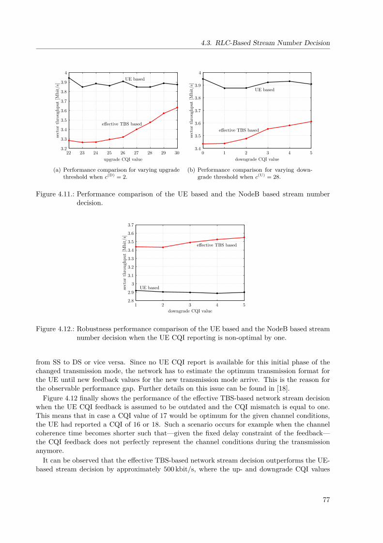
4.3. RLC-Based Stream Number Decision
22 23 24 25 26 27 28 29 303.2
3.3
3.4
3.5
3.6
3.7
3.8
3.9
4
sect
or t
hrou
ghpu
t [M
bit/
s]
upgrade CQI value
UE based
effective TBS based
(a) Performance comparison for varying upgradethreshold when c(D) = 2.
0 1 2 3 4 53.4
3.5
3.6
3.7
3.8
3.9
4
sect
or t
hrou
ghpu
t [M
bit/
s]
downgrade CQI value
UE based
effective TBS based
(b) Performance comparison for varying down-grade threshold when c(U) = 28.
Figure 4.11.: Performance comparison of the UE based and the NodeB based stream numberdecision.
1 2 3 4 52.8
2.9
3
3.1
3.2
3.3
3.4
3.5
3.6
3.7
sect
or t
hrou
ghpu
t [M
bit/
s]
downgrade CQI value
UE based
effective TBS based
Figure 4.12.: Robustness performance comparison of the UE based and the NodeB based streamnumber decision when the UE CQI reporting is non-optimal by one.
from SS to DS or vice versa. Since no UE CQI report is available for this initial phase of thechanged transmission mode, the network has to estimate the optimum transmission format forthe UE until new feedback values for the new transmission mode arrive. This is the reason forthe observable performance gap. Further details on this issue can be found in [18].
Figure 4.12 finally shows the performance of the effective TBS-based network stream decisionwhen the UE CQI feedback is assumed to be outdated and the CQI mismatch is equal to one.This means that in case a CQI value of 17 would be optimum for the given channel conditions,the UE had reported a CQI of 16 or 18. Such a scenario occurs for example when the channelcoherence time becomes shorter such that—given the fixed delay constraint of the feedback—the CQI feedback does not perfectly represent the channel conditions during the transmissionanymore.
It can be observed that the effective TBS-based network stream decision outperforms the UE-based stream decision by approximately 500 kbit/s, where the up- and downgrade CQI values
77
Chapter 4. System-Level-Simulation-Based Optimization of MIMO-Enhanced HSDPA
were set to 30 and 5, respectively. The main reason for this improved performance is that incase of non-perfect UE feedback, no control mechanism is left to ensure an average ACK/NACKratio of 0.1. The effective TBS-based algorithm however implicitly tries to maximize the sectorthroughput that can be delivered successfully. With the up- and downgrade thresholds setaccordingly, the network is able to stabilize effects that would increase the ACK/NACK ratio.
4.4. Content-Aware Scheduling
As already mentioned in the beginning of this chapter, system-level modeling and simulationcan also be utilized to perform cross-layer optimizations. In this section I restate the basicfindings of two contributions [19,20] that are based on investigations with the developed HSDPAsystem-level simulator to assess the performance of a Content-Aware (CA) cross-layer scheduler.
4.4.1. Introduction
The increase in available downlink data-rate and the developments in the core network archi-tecture make IP traffic in wireless networks more and more important. This traffic consists of avariety of different applications with different degrees of interactivity and technical needs. Thus3GPP standards define four classes of IP traffic [118], see Appendix A.9.1. These classes havebeen introduced to ensure certain QoS goals of the customers. However the QoS does not neces-sarily reflect the QoE [119] of the user. In particular for video applications, stringent constraintsin average data-rate, delay, jitter, or data-rate variance do not necessarily map one-to-one to theQoE. Since the QoE finally also determines the users’ willingness to pay for certain entertain-ment services applying it as a metric for network optimization seems intuitive. Accordingly, thissection is devoted to introduce a CA scheduler trying to maximize the QoE of the user and toassess its performance.
4.4.2. Video Packet Prioritization in HSDPA
Content awareness of the NodeB scheduler requires the signaling of content information to theMAC-hs layer. In particular, the importance of the encoded slice can then also be signaledexploiting the fields of the Network Abstract Layer (NAL) unit header [120]. At the videostreaming server, this priority information can be conveyed to the IP layer. The IP headercontains a byte originally designed to specify the Type Of Service (TOS) which is currently usedfor Differentiate Service (DiffServ) marking [121]. This specifies how a packet has to be handledby each network element.
UTRAN networks provide so called Packet Data Protocol (PDP) contexts to identify andarrange different packet switched connections. Within this method, the user terminal at oneside and the GGSN at the other side agree on several parameters, for example the IP address,the PDP type and the QoS profile of the following packets. Each PDP context supports oneQoS parameter setting at a time. The QoS information of the corresponding PDP contexts isalso available to the MAC-hs layer. To allow for multiple services with different requirementsdedicated to one user terminal to run in parallel, multiple PDP contexts are allowed in UMTS.
The basic idea of the cross layer signalization of the video content information is to encapsulatethe video packet information in the DiffServ field of the IP header. This information then is passedto the GGSN which, when establishing the PDP contexts to the desired user will establish a set
78
4.4. Content-Aware Scheduling
of PDP contexts,14 one for each priority class of the video content. According to the Traffic FlowTemplate (TFT) filter15 required at the GGSN for the operation of the multiple PDP contexts,the incoming IP packets will be filled in the corresponding flows. The MAC-hs scheduler then cantreat these packets arriving through different flows differently, enabling CA scheduling. Furtherdetails on the content information delivery from IP to MAC-hs layer can be found in [20].
4.4.3. Content-Aware SchedulerWith the IP packet priority information made available at the MAC-hs scheduler in the NodeB,the question remains how to exploit this information. The basic idea is to protect packets ofhigher importance for the QoE when decoded and displayed at the user terminal better againsttransmission errors. Simultaneously the scheduler shall have the flexibility to downgrade theerror protection on the physical layer for packets with less priority.
As explained in Chapter 2 and elaborated in Section 4.3, in HSDPA the NodeB has to adaptthe transmission settings according to the feedback information of the UEs, c(F). As a matterof fact, if the same quantized set of transmission formats as the table of feedback CQI values isutilized, the NodeB has to perform the mapping
T : c(F) → c(T), (4.15)
from feedback CQI c(F) to the transmit CQI c(T) representing the applied code-rate and modu-lation alphabet utilized for the transmission.
The proposed scheduler introduces an adaptive mapping, depending on the video packet pri-ority. Better protection can be achieved by remapping the transmit CQI to lower values and viceversa. However, if the transmit CQI is lowered to much, the average sector throughput woulddecrease notifiable which is in general undesired because spectral resources would be wasted.
As elaborated in Appendix A.9, packets belonging to I-frames contribute significantly to theoverall video quality, whereas packets belonging to P-frames influence it not that prominent. Inparticular this holds true for packets of P-frames that are at the end of a Group Of Pictures(GOP). Also note that in average one I-frame corresponds to four P-frames in size. Given theseQoE priority information, three scheduling priority classes can be defined
• priority ν = 2: packets belonging to I-frames,• priority ν = 1: packets belonging to the first (lGOP − 4) P-frames of the GOP,• priority ν = 0: packets belonging to the last 4 P-frames of the GOP,
where LGOP denotes the length of the GOP in frames. Then the proposed transmission mappingT of the MAC-hs scheduler is given by
Tν : c(T) = c(F) + 1− ν. (4.16)
To ensure fairness among all active users in the cell, the scheduler selects the served useraccording to a RR strategy. In addition, the maximum packet delay of the network has beenlimited by allowing a maximum number of one HARQ retransmission.14Let me note that the desired video content signaling requires the setup of one primary and a set of secondary
PDP contexts. The full treatment of this interrelation would be beyond the scope of this thesis, however furtherinformation can be found in [20].
15A TFT filter specifies a set of rules to assign incoming packets to PDP contexts. Details about the design ofthese filters can be found in [19].
79
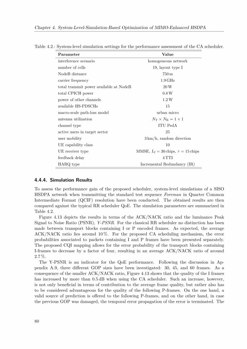
Chapter 4. System-Level-Simulation-Based Optimization of MIMO-Enhanced HSDPA
Table 4.2.: System-level simulation settings for the performance assessment of the CA scheduler.Parameter Valueinterference scenario homogeneous networknumber of cells 19, layout type INodeB distance 750 mcarrier frequency 1.9 GHztotal transmit power available at NodeB 20 Wtotal CPICH power 0.8 Wpower of other channels 1.2 Wavailable HS-PDSCHs 15macro-scale path-loss model urban microantenna utilization NT ×NR = 1× 1channel type ITU PedAactive users in target sector 25user mobility 3 km/h, random directionUE capability class 10UE receiver type MMSE, Lf = 30 chips, τ = 15 chipsfeedback delay 4 TTIHARQ type Incremental Redundancy (IR)
4.4.4. Simulation Results
To assess the performance gain of the proposed scheduler, system-level simulations of a SISOHSDPA network when transmitting the standard test sequence Foreman in Quarter CommonIntermediate Format (QCIF) resolution have been conducted. The obtained results are thencompared against the typical RR scheduler QoE. The simulation parameters are summarized inTable 4.2.
Figure 4.13 depicts the results in terms of the ACK/NACK ratio and the luminance PeakSignal to Noise Ratio (PSNR), Y-PSNR. For the classical RR scheduler no distinction has beenmade between transport blocks containing I or P encoded frames. As expected, the averageACK/NACK ratio lies around 10 %. For the proposed CA scheduling mechanism, the errorprobabilities associated to packets containing I and P frames have been presented separately.The proposed CQI mapping allows for the error probability of the transport blocks containingI-frames to decrease by a factor of four, resulting in an average ACK/NACK ratio of around2.7 %.
The Y-PSNR is an indicator for the QoE performance. Following the discussion in Ap-pendix A.9, three different GOP sizes have been investigated: 30, 45, and 60 frames. As aconsequence of the smaller ACK/NACK ratio, Figure 4.13 shows that the quality of the I frameshas increased by more than 0.5 dB when using the CA scheduler. Such an increase, however,is not only beneficial in terms of contribution to the average frame quality, but rather also hasto be considered advantageous for the quality of the following P-frames. On the one hand, avalid source of prediction is offered to the following P-frames, and on the other hand, in casethe previous GOP was damaged, the temporal error propagation of the error is terminated. The
80
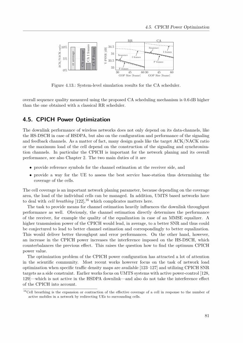
4.5. CPICH Power Optimization
0%
5%
10%
rr a
vera
ge
CA
ave
rage
CA
I fra
mes
CA
P fra
mes
AC
K/N
AC
K r
atio
33
33.5
34
34.5
30 6045 30 6045GOP Size [frame] GOP Size [frame]
Y-P
SNR
[dB
]
I frames
I framesSequence
Sequence
P frames
P frames
RR CA
Figure 4.13.: System-level simulation results for the CA scheduler.
overall sequence quality measured using the proposed CA scheduling mechanism is 0.6 dB higherthan the one obtained with a classical RR scheduler.
4.5. CPICH Power Optimization
The downlink performance of wireless networks does not only depend on its data-channels, likethe HS-DSCH in case of HSDPA, but also on the configuration and performance of the signalingand feedback channels. As a matter of fact, many design goals like the target ACK/NACK ratioor the maximum load of the cell depend on the construction of the signaling and synchroniza-tion channels. In particular the CPICH is important for the network planing and its overallperformance, see also Chapter 2. The two main duties of it are
• provide reference symbols for the channel estimation at the receiver side, and• provide a way for the UE to assess the best service base-station thus determining the
coverage of the cells.
The cell coverage is an important network planing parameter, because depending on the coveragearea, the load of the individual cells can be managed. In addition, UMTS based networks haveto deal with cell breathing [122],16 which complicates matters here.
The task to provide means for channel estimation heavily influences the downlink throughputperformance as well. Obviously, the channel estimation directly determines the performanceof the receiver, for example the quality of the equalization in case of an MMSE equalizer. Ahigher transmission power of the CPICH would lead, in average, to a better SNR and thus couldbe conjectured to lead to better channel estimation and correspondingly to better equalization.This would deliver better throughput and error performances. On the other hand, however,an increase in the CPICH power increases the interference imposed on the HS-DSCH, whichcounterbalances the previous effect. This raises the question how to find the optimum CPICHpower value.
The optimization problem of the CPICH power configuration has attracted a lot of attentionin the scientific community. Most recent works however focus on the task of network loadoptimization when specific traffic density maps are available [123–127] and utilizing CPICH SNRtargets as a side constraint. Earlier works focus on UMTS systems with active power-control [128,129]—which is not active in the HSDPA downlink—and also do not take the interference effectof the CPICH into account.16Cell breathing is the expansion or contraction of the effective coverage of a cell in response to the number of
active mobiles in a network by redirecting UEs to surrounding cells.
81
Chapter 4. System-Level-Simulation-Based Optimization of MIMO-Enhanced HSDPA
In this section I restate the basic findings of my efforts to solve the CPICH power optimizationproblem for HSDPA networks. This work is based on an enhancement of the link-quality modelof Chapter 3 to reflect the influence of the CPICH and utilizes the HSDPA system-level simulatorto evaluate the optimum CPICH power values [21].
4.5.1. System-Level Modeling of the CPICH InfluenceTo numerically assess the influence of the CPICH on the performance of the HS-DSCH, thelink-quality model of Chapter 3 has to be refined. So far, always perfect CSI at the UE had beenassumed.
Before going into the details on the link-quality model enhancement, let me spent a few wordson the CPICH. UMTS based networks offer two different CPICHs, the primary and the secondaryCPICH, where the secondary one is designed to serve dedicated hot spot areas and thus will beneglected in the following. The primary CPICH has the following features:
• the spreading sequence for the primary CPICH is always the same with length 256,• there is only one primary CPICH in the cell that is broadcasted over the whole cell area,
and• 4-QAM modulation is utilized, which results in a bit-rate of 30 kbit/s.
A detailed description of the primary and secondary CPICH including the channel coding andscrambling sequence details can be found in [34]. In the following, let me denote the primaryCPICH only by the name CPICH for sake of notational simplicity.
Link-Quality Model Enhancement
To integrate the CPICH influence in the link-quality model, the employed receive filter—in thiswork the MMSE equalizer from Equation (3.14)—has to be based on the estimated channel. Inparticular, if the estimated channel is denoted by ˆHw, the MMSE equalizer is given by
F = RxSi−τ xi
ˆHHw
( ˆHwRxiˆHH
w + Rni
)−1. (4.17)
As investigated in [21], the estimated channel ˆHw can statistically be represented by the matrix
ˆHw = Hw + H∆, (4.18)
with the error matrix H∆ being of the same structure like Hw. This means that H∆ hasto be generated according to H∆ , σ2
MSEG, with G being a random Gaussian matrix of thesame frequency selectivity structure like Hw with variance one. The variance σ2
MSE specifies theweighting of the error matrix and is a function of the CPICH transmission power. Accordingly,the equivalent fading parameters can easily be generated utilizing F instead of F for variousCPICH transmission power values.
Modeling Validation
To validate the new equivalent fading parameters, a set of link level simulations has been per-formed for different antenna configurations, comparing the true SINR as evaluated in Equa-tion (3.65) with the SINR as predicted by the modeling. Figure 4.14 shows the resulting model
82
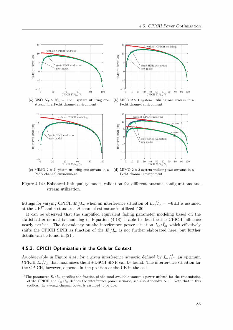
4.5. CPICH Power Optimization
0 20 40 60 80 100−10
−5
0
5
10
15
HS-
DSC
H S
INR
[dB
]
without CPICH modeling
genie SINR evaluationnew model
(a) SISO NT × NR = 1 × 1 system utilizing onestream in a PedA channel environment.
0 10 20 30 40 50 60 70 80 90 100−10
−5
0
5
10
15
HS-
DSC
H S
INR
[dB
]
without CPICH modeling
genie SINR evaluationnew model
(b) MISO 2 × 1 system utilizing one stream in aPedA channel environment.
0 20 40 60 80 100−5
0
5
10
15
20
HS-
DSC
H S
INR
[dB
]
without CPICH modeling
genie SINR evaluationnew model
(c) MIMO 2 × 2 system utilizing one stream in aPedA channel environment.
0 10 20 30 40 50 60 70 80 90 100−15
−10
−5
0
5
10
15
H
S-D
SCH
SIN
R [dB
]without CPICH modeling
genie SINR evaluationnew model
stream 1
stream 2
(d) MIMO 2 × 2 system utilizing two streams in aPedA channel environment.
Figure 4.14.: Enhanced link-quality model validation for different antenna configurations andstream utilization.
fittings for varying CPICH Ec/Ior when an interference situation of Ioc/Ior = −6 dB is assumedat the UE17 and a standard LS channel estimator is utilized [130].
It can be observed that the simplified equivalent fading parameter modeling based on thestatistical error matrix modeling of Equation (4.18) is able to describe the CPICH influencenearly perfect. The dependency on the interference power situation Ioc/Ior which effectivelyshifts the CPICH SINR as function of the Ec/Ior is not further elaborated here, but furtherdetails can be found in [21].
4.5.2. CPICH Optimization in the Cellular Context
As observable in Figure 4.14, for a given interference scenario defined by Ioc/Ior an optimumCPICH Ec/Ior that maximizes the HS-DSCH SINR can be found. The interference situation forthe CPICH, however, depends in the position of the UE in the cell.17The parameter Ec/Ior specifies the fraction of the total available transmit power utilized for the transmission
of the CPICH and Ioc/Ior defines the interference power scenario, see also Appendix A.11. Note that in thissection, the average channel power is assumed to be one.
83
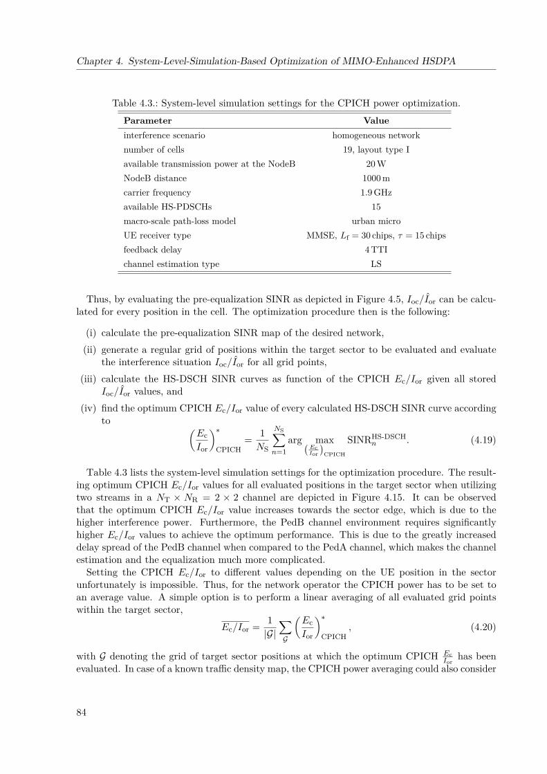
Chapter 4. System-Level-Simulation-Based Optimization of MIMO-Enhanced HSDPA
Table 4.3.: System-level simulation settings for the CPICH power optimization.Parameter Valueinterference scenario homogeneous networknumber of cells 19, layout type Iavailable transmission power at the NodeB 20 WNodeB distance 1000 mcarrier frequency 1.9 GHzavailable HS-PDSCHs 15macro-scale path-loss model urban microUE receiver type MMSE, Lf = 30 chips, τ = 15 chipsfeedback delay 4 TTIchannel estimation type LS
Thus, by evaluating the pre-equalization SINR as depicted in Figure 4.5, Ioc/Ior can be calcu-lated for every position in the cell. The optimization procedure then is the following:
(i) calculate the pre-equalization SINR map of the desired network,(ii) generate a regular grid of positions within the target sector to be evaluated and evaluate
the interference situation Ioc/Ior for all grid points,(iii) calculate the HS-DSCH SINR curves as function of the CPICH Ec/Ior given all stored
Ioc/Ior values, and(iv) find the optimum CPICH Ec/Ior value of every calculated HS-DSCH SINR curve according
to (EcIor
)∗CPICH
= 1NS
NS∑n=1
arg max(EcIor
)CPICH
SINRHS-DSCHn . (4.19)
Table 4.3 lists the system-level simulation settings for the optimization procedure. The result-ing optimum CPICH Ec/Ior values for all evaluated positions in the target sector when utilizingtwo streams in a NT × NR = 2 × 2 channel are depicted in Figure 4.15. It can be observedthat the optimum CPICH Ec/Ior value increases towards the sector edge, which is due to thehigher interference power. Furthermore, the PedB channel environment requires significantlyhigher Ec/Ior values to achieve the optimum performance. This is due to the greatly increaseddelay spread of the PedB channel when compared to the PedA channel, which makes the channelestimation and the equalization much more complicated.
Setting the CPICH Ec/Ior to different values depending on the UE position in the sectorunfortunately is impossible. Thus, for the network operator the CPICH power has to be set toan average value. A simple option is to perform a linear averaging of all evaluated grid pointswithin the target sector,
Ec/Ior = 1|G|
∑G
(EcIor
)∗CPICH
, (4.20)
with G denoting the grid of target sector positions at which the optimum CPICH EcIor
has beenevaluated. In case of a known traffic density map, the CPICH power averaging could also consider
84

4.6. Summary
0200
400600
−200−1000
100200
0
5
10
15
20
25
30
distance NodeB-UE [m]
optim
um C
PIC
H[%
]
distance NodeB-UE [m]
(a) MIMO NT ×NR = 2× 2 network utilizing twostreams in a PedA channel environment.
0200
400600
−200−1000
100200
0
5
10
15
20
25
30
distance NodeB-UE [m]
optim
um C
PIC
H[%
]
distance NodeB-UE [m]
(b) MIMO 2× 2 network utilizing two streams in aPedB channel environment.
Figure 4.15.: DS utilization CPICH power optimization results for different antenna configura-tions experiencing PedA and PedB channel environments, respectively.
Table 4.4.: Resulting optimum average CPICH Ec/Ior values for different network configurationsand channel profiles.
Network configuration Ec/Ior [%]MISO 2× 1, TxAA, PedA 11.00MISO 2× 1, TxAA, PedB 19.92MIMO 2× 2, TxAA, PedA 13.08MIMO 2× 2, TxAA, PedB 21.08MIMO 2× 2, D-TxAA, PedA 14.67MIMO 2× 2, D-TxAA, PedB 21.75
this density distribution. The resulting optimum average CPICH Ec/Ior values for all evaluatednetwork scenarios are listed in Table 4.4.
Finally, let me note that the presented optimization procedure neglects CPICH pollution ef-fects [131] which can cause problems for the UMTS soft handover. To reflect these optimizationconstraints target CPICH SINR values at the cell edge would have to be defined. Nevertheless,the resulting optimum CPICH power values can serve as a design guideline for HSDPA networksgiven different antenna configurations and may be particularly helpful for when MIMO networksare put in trial.
4.6. SummarySystem-level simulations can serve as a flexible design and test tool for network performanceevaluation, algorithm development, and deployment optimization. In this chapter, I presented apossible concept for a MIMO HSDPA network simulator, building upon the system-level modelproposed in Chapter 3. Furthermore, four exemplary applications of the simulator were elabo-rated.
By means of a system-level simulation campaign, network performance predictions for various
85
Chapter 4. System-Level-Simulation-Based Optimization of MIMO-Enhanced HSDPA
deployment scenarios were obtained. I also shortly discussed the consequences of the D-TxAAdouble-stream operation onto the fairness in the network. On top of that I also proposed arobust RLC stream allocation algorithm and a content-aware scheduler improving the QoE. Bothalgorithms have been tested by extensive system-level simulations. Finally, optimum CPICHpower allocations maximizing the HSDPA link quality for many different network setups havebeen evaluated.
Although fairly general in its concept, the system-level simulator could benefit significantlyfrom a more structured implementation. In fact, developing a software of this extend in Matlabis in general quite demanding because the Integrated Development Environment (IDE) is notwell suited for such a task. Recently, however, Matlab introduced object-orientated languageextensions providing more flexibility for larger projects. If the simulator were structured ac-cording to these new possibilities, extensions to the core functionality would be much easier toimplement.
Regarding the channel modeling in the network context, two assumptions worth researchingshall be commented. At the moment, the utilized channel model is based on a constant PDP,for example according to the ITU channel profile. However, measurements show that the delayspread becomes smaller with shorter distance to the NodeB. This behavior is currently not rep-resented and would require more sophisticated channel models as well as a refined representationof the equivalent fading parameters. In this context, also a better understanding of the outdoor-to-indoor MIMO channel would help to predict the network performance more realistically. Alsorefined possibilities in antenna deployment optimization, 3-D antenna gain patterns would haveto be implemented. Moreover, it would be of great scientific interest to more rigorously defineand assess the connection of classical performance metrics like throughput with fairness. Inparticular, modern MU optimized transmission systems have to put more focus on fairness cri-teria. To give better planing guidelines to the network operators, the system-level optimizationsshould incorporate cell-edge target constraints because usually certain QoS requirements haveto be met. In terms of the physical layer investigations in the network context, it would alsobe very interesting to assess potential performance gains due to MU stream allocation, that is,serving two users simultaneously by means of SDMA [132]. For the content-aware scheduler,future research would have to put focus on how to incorporate the PF user utility function. Itwould also be of interest to investigate how to extend the applicability of the proposed sched-uler to the multi-stream D-TxAA transmission mode. Finally, a full analytical modeling of theCPICH power influence on the system performance would be of great interest. This would allowto utilize convex optimization theory to develop dynamic allocation algorithms.
From a theoretical point of view, the definition and the evaluation of the cell-capacity wouldbe of great importance. So far, no theoretical results can be used as a capacity metric to compareagainst the obtained system-level results. Appendix A.8 lists some initial ideas in this context,but detailed knowledge about this topic is needed to understand the fundamental performancelimits of any scheduler and to define and compare against the optimum network.
At last, let me point out that a validation of a system-level simulator is in general verydemanding. Usually, link-level simulators are not designed to include inter-cell and possiblyinter-technology interference necessary. For future mobile networks, it thus would be beneficialif the underlying link-level simulator used to derive parts of the physical-layer abstraction canbe utilized to simulate certain network test-scenarios against which the system-level simulatorcan be validated. In the scope of this work, at least a validation against the mobilkom austriaAG trial data was performed in Appendix A.13, showing a good match. However, with a set oftest-simulation setups a much more comprehensive validation would be possible.
86

Chapter 5.
Multi-User MMSE Equalization forMIMO-Enhanced HSDPA
The structure will automaticallyprovide the pattern for the actionwhich follows.
(Donald Curtis)
Interference is said to be the most important performance limiting factor of modern cellularcommunication systems. This especially holds true for WCDMA networks, where frequency
selectivity in the downlink channel causes a loss in orthogonality between the utilized spreadingcodes and imposes restrictive throughput constraints. This issue has already been identified inChapter 3 for the development of the link-quality model, as well as in the simulation results inChapter 4. However, besides the unavoidable interference caused by spreading code crosstalk, thequestion arises whether there exist possibilities to exploit structural properties in the interferencefor MIMO HSDPA.
The information theoretic principles for this kind of interference problem are represented bythe MIMO broadcast channel [133, 134], which is related to the MIMO multiple-access channelin the uplink [135]. Although the capacity regions in case of fading channels are not known yet,all of the results so far indicate the need for interference mitigation to come close to the upperbound on the sum-capacity [136,137].
Interference can be combated at the transmitter and/or the receiver side. In particular, in thedownlink each receiver needs to detect a single desired signal, while experiencing two main typesof interference. These are caused by the serving NodeB, called intra-cell interference, and bya few dominant neighboring NodeBs, called inter-cell interference. In the uplink, on the otherhand, the base station receiver has to detect all desired users in the cell while having to suppressneighboring interference from many different sources.
When interference mitigation is performed at the transmitter, accurate channel state informa-tion from all users is needed [138]. The optimum solution known so far for the multi-user caseis the utilization of Dirty Paper Coding (DPC) [139], which requires full channel and transmitsignal knowledge at a central coordinating entity. A generalization of the classical DPC idea tothe case of multiple base-stations has been made in [140]. This requires lots of signaling andfeedback information exchange, which is typically not available in cellular context. Beamformingmay serve as an approximation to the optimum interference mitigation at the transmitter, butfaces some theoretical difficulties [141].
Handling the interference on the receiver side is a difficult job as well, especially in the multi-user case where classical approaches result in complex receiver structures [142–144]. Moreover,also theoretically it is not known to which extend receiver cooperation is needed to achieve a closeto capacity performance, apart from the fact that it is not known what the optimum receiver
87
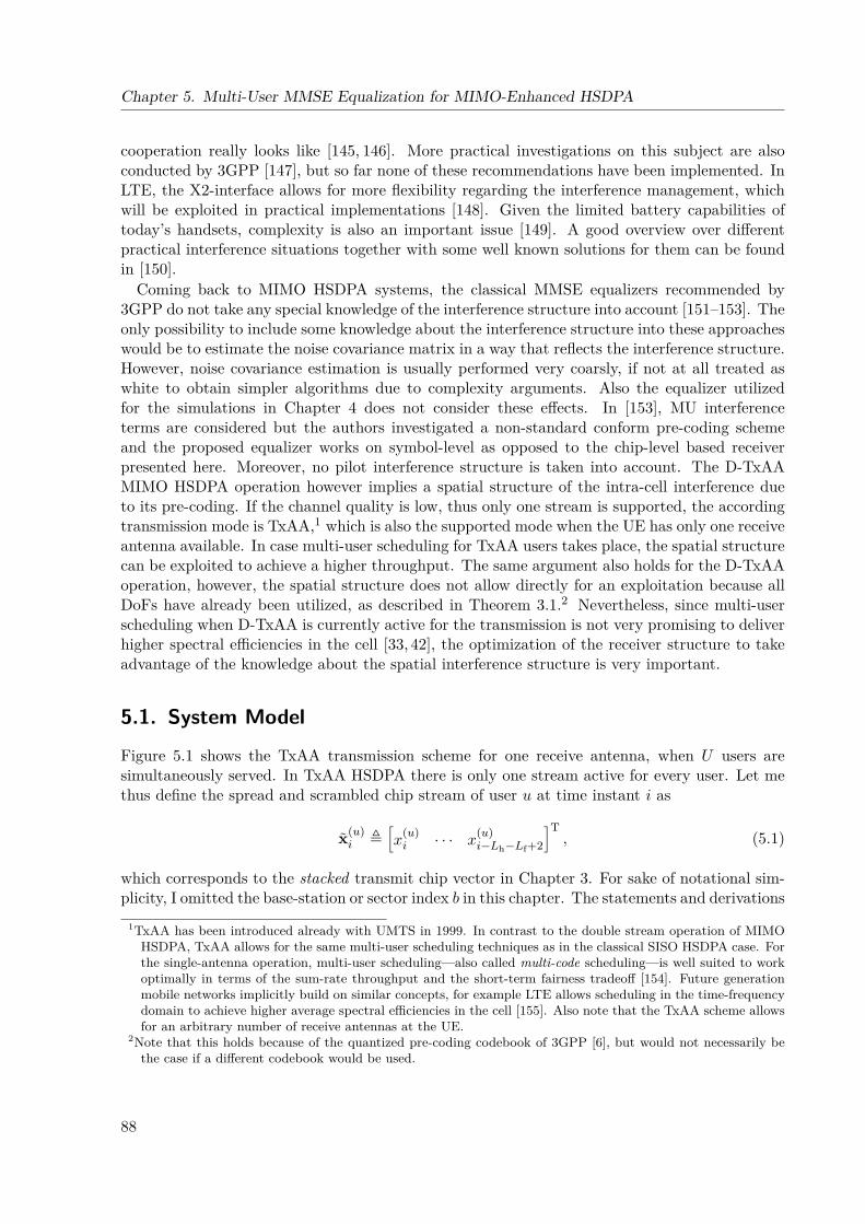
Chapter 5. Multi-User MMSE Equalization for MIMO-Enhanced HSDPA
cooperation really looks like [145, 146]. More practical investigations on this subject are alsoconducted by 3GPP [147], but so far none of these recommendations have been implemented. InLTE, the X2-interface allows for more flexibility regarding the interference management, whichwill be exploited in practical implementations [148]. Given the limited battery capabilities oftoday’s handsets, complexity is also an important issue [149]. A good overview over differentpractical interference situations together with some well known solutions for them can be foundin [150].
Coming back to MIMO HSDPA systems, the classical MMSE equalizers recommended by3GPP do not take any special knowledge of the interference structure into account [151–153]. Theonly possibility to include some knowledge about the interference structure into these approacheswould be to estimate the noise covariance matrix in a way that reflects the interference structure.However, noise covariance estimation is usually performed very coarsly, if not at all treated aswhite to obtain simpler algorithms due to complexity arguments. Also the equalizer utilizedfor the simulations in Chapter 4 does not consider these effects. In [153], MU interferenceterms are considered but the authors investigated a non-standard conform pre-coding schemeand the proposed equalizer works on symbol-level as opposed to the chip-level based receiverpresented here. Moreover, no pilot interference structure is taken into account. The D-TxAAMIMO HSDPA operation however implies a spatial structure of the intra-cell interference dueto its pre-coding. If the channel quality is low, thus only one stream is supported, the accordingtransmission mode is TxAA,1 which is also the supported mode when the UE has only one receiveantenna available. In case multi-user scheduling for TxAA users takes place, the spatial structurecan be exploited to achieve a higher throughput. The same argument also holds for the D-TxAAoperation, however, the spatial structure does not allow directly for an exploitation because allDoFs have already been utilized, as described in Theorem 3.1.2 Nevertheless, since multi-userscheduling when D-TxAA is currently active for the transmission is not very promising to deliverhigher spectral efficiencies in the cell [33, 42], the optimization of the receiver structure to takeadvantage of the knowledge about the spatial interference structure is very important.
5.1. System Model
Figure 5.1 shows the TxAA transmission scheme for one receive antenna, when U users aresimultaneously served. In TxAA HSDPA there is only one stream active for every user. Let methus define the spread and scrambled chip stream of user u at time instant i as
x(u)i ,
[x
(u)i · · · x
(u)i−Lh−Lf+2
]T, (5.1)
which corresponds to the stacked transmit chip vector in Chapter 3. For sake of notational sim-plicity, I omitted the base-station or sector index b in this chapter. The statements and derivations
1TxAA has been introduced already with UMTS in 1999. In contrast to the double stream operation of MIMOHSDPA, TxAA allows for the same multi-user scheduling techniques as in the classical SISO HSDPA case. Forthe single-antenna operation, multi-user scheduling—also called multi-code scheduling—is well suited to workoptimally in terms of the sum-rate throughput and the short-term fairness tradeoff [154]. Future generationmobile networks implicitly build on similar concepts, for example LTE allows scheduling in the time-frequencydomain to achieve higher average spectral efficiencies in the cell [155]. Also note that the TxAA scheme allowsfor an arbitrary number of receive antennas at the UE.
2Note that this holds because of the quantized pre-coding codebook of 3GPP [6], but would not necessarily bethe case if a different codebook would be used.
88
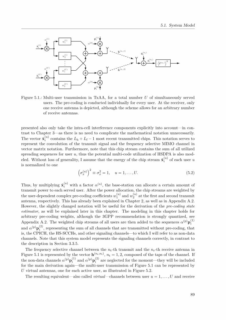
5.1. System Model
Figure 5.1.: Multi-user transmission in TxAA, for a total number U of simultaneously servedusers. The pre-coding is conducted individually for every user. At the receiver, onlyone receive antenna is depicted, although the scheme allows for an arbitrary numberof receive antennas.
presented also only take the intra-cell interference components explicitly into account—in con-trast to Chapter 3—as there is no need to complicate the mathematical notation unnecessarily.The vector x(u)
i contains the Lh + Lf − 1 most recent transmitted chips. This notation serves torepresent the convolution of the transmit signal and the frequency selective MIMO channel invector matrix notation. Furthermore, note that this chip stream contains the sum of all utilizedspreading sequences for user u, thus the potential multi-code utilization of HSDPA is also mod-eled. Without loss of generality, I assume that the energy of the chip stream x(u)
i of each user uis normalized to one (
σ(u)x
)2≡ σ2
x = 1, u = 1, . . . , U. (5.2)
Thus, by multiplying x(u)i with a factor α(u), the base-station can allocate a certain amount of
transmit power to each served user. After the power allocation, the chip streams are weighted bythe user-dependent complex pre-coding coefficients w(u)
1 and w(u)2 at the first and second transmit
antenna, respectively. This has already been explained in Chapter 2, as well as in Appendix A.2.However, the slightly changed notation will be useful for the derivation of the pre-coding stateestimator, as will be explained later in this chapter. The modeling in this chapter holds forarbitrary pre-coding weights, although the 3GPP recommendation is strongly quantized, seeAppendix A.2. The weighted chip streams of all users are then added to the sequences α(p)p(1)
i
and α(p)p(2)i , representing the sum of all channels that are transmitted without pre-coding, that
is, the CPICH, the HS-SCCHs, and other signaling channels—to which I will refer to as non-datachannels. Note that this system model represents the signaling channels correctly, in contrast tothe description in Section 3.3.5.
The frequency selective channel between the nt-th transmit and the nr-th receive antenna inFigure 5.1 is represented by the vector h(nr,nt), nt = 1, 2, composed of the taps of the channel. Ifthe non-data channels α(p)p(1)
i and α(p)p(2)i are neglected for the moment—they will be included
for the main derivation again—the multi-user transmission of Figure 5.1 can be represented byU virtual antennas, one for each active user, as illustrated in Figure 5.2.
The resulting equivalent—also called virtual—channels between user u = 1, . . . , U and receive
89
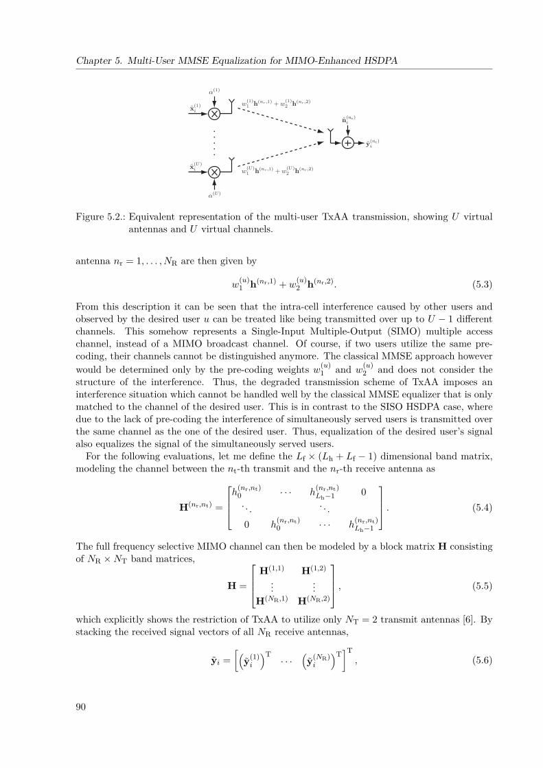
Chapter 5. Multi-User MMSE Equalization for MIMO-Enhanced HSDPA
Figure 5.2.: Equivalent representation of the multi-user TxAA transmission, showing U virtualantennas and U virtual channels.
antenna nr = 1, . . . , NR are then given by
w(u)1 h(nr,1) + w
(u)2 h(nr,2). (5.3)
From this description it can be seen that the intra-cell interference caused by other users andobserved by the desired user u can be treated like being transmitted over up to U − 1 differentchannels. This somehow represents a Single-Input Multiple-Output (SIMO) multiple accesschannel, instead of a MIMO broadcast channel. Of course, if two users utilize the same pre-coding, their channels cannot be distinguished anymore. The classical MMSE approach howeverwould be determined only by the pre-coding weights w(u)
1 and w(u)2 and does not consider the
structure of the interference. Thus, the degraded transmission scheme of TxAA imposes aninterference situation which cannot be handled well by the classical MMSE equalizer that is onlymatched to the channel of the desired user. This is in contrast to the SISO HSDPA case, wheredue to the lack of pre-coding the interference of simultaneously served users is transmitted overthe same channel as the one of the desired user. Thus, equalization of the desired user’s signalalso equalizes the signal of the simultaneously served users.
For the following evaluations, let me define the Lf × (Lh + Lf − 1) dimensional band matrix,modeling the channel between the nt-th transmit and the nr-th receive antenna as
H(nr,nt) =
h
(nr,nt)0 · · · h
(nr,nt)Lh−1 0
. . . . . .0 h
(nr,nt)0 · · · h
(nr,nt)Lh−1
. (5.4)
The full frequency selective MIMO channel can then be modeled by a block matrix H consistingof NR ×NT band matrices,
H =
H(1,1) H(1,2)
......
H(NR,1) H(NR,2)
, (5.5)
which explicitly shows the restriction of TxAA to utilize only NT = 2 transmit antennas [6]. Bystacking the received signal vectors of all NR receive antennas,
yi =[(
y(1)i
)T· · ·
(y(NR)i
)T]T, (5.6)
90
5.2. Intra-Cell Interference-Aware MMSE Equalization
and by stacking the transmitted signal vectors of all U users and the auxiliary channel signalvectors p(1)
i and p(2)i ,
xi =[(
x(1)i
)T· · ·
(x(U)i
)T (p(1)i
)T (p(2)i
)T]T, (5.7)
the compact system description follows as
yi = H(W(MU) ⊗ ILh+Lf−1
)xi + ni = Hwxi + ni. (5.8)
In this formulation, ni can be used to incorporate both the thermal noise and the inter-cell inter-ference from other base-stations, which would allow the resulting receive filter some possibilitiesto combat the inter-cell interference as well.
The 2× (U + 2) dimensional matrix W(MU) contains the pre-coding coefficients w(u)1 and w(u)
2of all users, as well as the power coefficients α(u),
W(MU) ,
[α(1)w
(1)1 · · · α(U)w
(U)1 α(p) 0
α(1)w(1)2 · · · α(U)w
(U)2 0 α(p)
]. (5.9)
This matrix reflects the premise that non-data channels are not pre-coded, thus the two columnson the right side are specified solely by the single parameter α(p) which controls the total powerspent on these channels. In general, I also assume that the power available at the base-stationis fully spent, thus the coefficients α are prone to a sum-power constraint,
∥∥∥W(MU)∥∥∥2
fro=
U∑u=1
(α(u)
)2+ 2
(α(p)
)2= P, (5.10)
with ‖ · ‖fro denoting the Frobenius norm. Furthermore, I assume the power control to becompletely included in the power coefficients α(u) and α(p) which imposes an additional powerconstraint on the pre-coding coefficients, ‖w(u)‖2 = 1 with w(u) , [w(u)
1 , w(u)2 ]T.
5.2. Intra-Cell Interference-Aware MMSE EqualizationHaving the system model being specified, the resulting MMSE equalizer can be derived. With-out loss of generality, I will assume that the transmit data sequence of user one has to bereconstructed. Accordingly, the MMSE equalizer coefficients can be calculated by minimizingthe quadratic cost function [89]
J(f) = E∣∣∣fHyi − x(1)
i−τ
∣∣∣2 , (5.11)
with τ again specifying the delay of the equalized signal, and fulfilling τ ≥ Lh.3 Similar toChapter 3, I will assume perfect channel knowledge at the receiver side here.
The cost function minimizes the distance between the equalized chip stream and the trans-mitted chip stream in the Euclidean distance sense. In Equation (5.11), the vector f defines NRequalization filters,
f =[(
f (1))T
· · ·(f (NR)
)T]T. (5.12)
3See Chapter 3 for details on this constraint.
91

Chapter 5. Multi-User MMSE Equalization for MIMO-Enhanced HSDPA
Each filter f (nr) =[f
(nr)0 · · · f
(nr)Lf−1
]has a length of Lf chips, similar to the equalizer derived
in Chapter 3. Note that because of the definition of f and yi, the inner product fHyi can beimplemented by summation of the outputs of the NR equalization filters f (nr). This sum thenyields the MMSE estimate of the transmitted chip sequence.
To obtain the optimum receive filter, the cost function J(f) has to be minimized,
f (opt) , arg minfJ(f) , (5.13)
which, due to the design of the cost-function, is a convex non-constraint optimization problem [92,156]. Accordingly, it can be solved by finding the point at which the gradient of the cost functionis equal to zero,
∇J(f (opt)
) != 0NRLf , (5.14)
with 0NRLf denoting a zero vector of length NRLf. Let me use the same definition of the complexderivative as in [157],4
z = x+ jy → ∂
∂z= 1
2
(∂
∂x− j ∂
∂y
),∂
∂z∗= 1
2
(∂
∂x+ j
∂
∂y
). (5.15)
Then it can be shown that the gradient problem can be reformulated to
∇J(f) = 2 ∂
∂f∗J(f) . (5.16)
By applying linearity of the expectation and the partial derivative operator, the gradient ofthe cost function can be shown to be
∂
∂f∗J(f) = E∂
∂f∗ fHyiyH
i f − x(1)i−τ y
Hi f − fHyi
(x
(1)i−τ
)∗+∣∣∣x(1)i−τ
∣∣∣2 , (5.17)
which becomes∂
∂f∗J(f) = EyiyH
i f − yi(x
(1)i−τ
)∗. (5.18)
Inserting the input-output relation from Equation (5.8) and assuming uncorrelated data andnoise samples, the derivative of the cost function can be further simplified to
∂
∂f∗J(f) =[HwE
xixH
i
HH
w + EninH
i
]f −HwE
xi(x
(1)i−τ
)∗, (5.19)
4Note that this definition also implies that
∂z
∂z= 1, ∂z
∂z∗= ∂z∗
∂z= 0,
for complex valued numbers z, as well as
∂z∂z = I, ∂z
∂z∗ = ∂z∗
∂z = 0
for complex valued vectors z. This definition extends the differentials to non-homomorphic functions in thecomplex numbers plane, where the Cauchy-Riemann equations do not hold anymore. A definition like this isnecessary because most functions encountered in physical sciences and engineering are not analytic. In themathematical literature, these relationships are often called Wirtinger calculus [158].
92
5.2. Intra-Cell Interference-Aware MMSE Equalization
which by defining Rxx , ExixH
i
and Rnn , E
ninH
i
, as well as assuming the individual
transmit chips to be uncorrelated,
Exi(x
(1)i−τ
)∗= E
∣∣∣x(1)i−τ
∣∣∣2 eτ = σ2xeτ , (5.20)
leads to∂J
∂f∗ =(HwRxxHH
w + Rnn
)f − σ2
xHweτ!= 0. (5.21)
The matrices Rxx and Rnn are the signal and noise covariance matrices, respectively, and thevector eτ is a zero vector of length (U + 2)(Lh + Lf − 1) with a single one at position τ . Theequalizer coefficients for the data stream of the first user are therefore given by
f = σ2x
(HwRxxHH
w + Rnn
)−1Hweτ . (5.22)
If the transmitted data signals of the users are uncorrelated with equal powers σ2x, the covariance
matrix Rxx becomes σ2xI, and if the noise vector ni is assumed white with variance σ2
n, the noisecovariance matrix becomes σ2
nI. As already mentioned, I will assume the transmit signal varianceto be equal to one, because the individual transmit powers of the users are anyways determinedby the power coefficients α(u). The variance σ2
n on the other hand is specified by the thermalnoise power and the sum interference power from the neighboring base-stations. Note that if thereceiver shall ideally take the structure of the inter-cell interference into account, effort wouldhave to be put into obtaining an accurate estimation of the covariance matrix Rnn, which wouldnot be a scaled identity matrix anymore.
Since this equalizer considers the interference of all users in the cell due to the full knowledge ofthe matrix W(MU), it can be called intra-cell interference aware MMSE equalizer. The standardequalizer is a special case of this solution and neglects the interference structure imposed by theother users, which I will call Single-User (SU) equalizer in the following. It can be calculatedfrom Equation (5.22) by utilizing the SU pre-coding weight matrix of rank one,
W(SU) =[α(1)w
(1)1
α(1)w(1)2
]eT
1 , (5.23)
instead of the multi-user matrix W(MU). Here, e1 is a zero column-vector of length U + 2 witha one at the first position. Note that if only a single user is receiving data in the cell bothequalizers are very similar. The only difference is that the intra-cell interference aware equalizeralso considers the interference generated by the non-data channels.
The structure of the derived linear equalizer would in principle also allow for an extension todecision-feedback receivers. However, if the interference caused by the other users is sought to becancelled, their data has to be estimated and thus the computational complexity of the resultingreceiver would be increased significantly. Furthermore, decision-feedback receivers suffer fromimpractical delay constraints due to the length of the spreading sequences in WCDMA systemsas well as error propagation.
5.2.1. Interference Suppression CapabilityHaving derived the solution of the interference-aware MMSE equalizer, it is of interest to an-alytically assess its interference-suppression capabilities as well as its performance bounds. To
93
Chapter 5. Multi-User MMSE Equalization for MIMO-Enhanced HSDPA
do so, I adapted the system-level link quality model introduced in Chapter 3 which is capa-ble of describing the post-equalization and despreading SINR for arbitrary linear receivers ina potentially multi-stream closed loop MIMO Code-Division Multiple Access (CDMA) system.The remaining intra-cell interference after equalization—for a specific channel realization andpre-coding state—generated by the desired user and all other active users is explicitly given by
P intra =Lh+Lf−2∑m=0m6=τ
∣∣∣fHh(1)m
∣∣∣2 +U∑u=2
Lh+Lf−2∑m=0
∣∣∣fHh(u)m
∣∣∣2 , (5.24)
where in reference to Equation (3.37) I set NS = 1 due to the restriction to the TxAA trans-mission mode, and the total transmission power per stream, P (u,b0)/NS is now incorporated inthe power coefficients α(u). These furthermore are contained in the equivalent MIMO channelmatrix columns h(u)
m of the user dedicated channel matrix
H(u) = H([α(u)w
(u)1 α(u)w
(u)2
]⊗ ILh+Lf−1
), (5.25)
where I assumed perfect channel and noise power knowledge at the receiver.Equation (5.24) depends on the current realization of the pre-coding state, in particular the
pre-coding choices of the interfering users. Thus to assess the average interference suppressioncapability of the proposed equalizer, I utilize the expected intra-cell interference5 which for acertain number of active users in the cell becomes
EwP intra
=
Lh+Lf−2∑m=0m 6=τ
∣∣∣fHh(1)m
∣∣∣2︸ ︷︷ ︸
fself
+U∑u=2
Ew
Lh+Lf−2∑m=0
∣∣∣fHh(u)m
∣∣∣2︸ ︷︷ ︸
fother
, (5.26)
with fself and fother denoting the determinative factors for the self- and other-user intra-cellinterference remaining after equalization, and Ew· being the expectation with respect to thepre-coding coefficients w1 and w2 of the other users.
Utilizing the analytical description of the post-equalization intra-cell interference the interfer-ence suppression capabilities and the theoretical performance bounds of the proposed equalizercan be evaluated. Table 5.1 lists the simulation parameters I applied to assess the capabilityof the proposed equalizer to suppress the intra-cell interference caused due to the other activeusers in the cell. Figure 5.3(a) shows the performance in terms of the interference suppressioncapabilities, both for the self interference fself, and the other-user interference fother, assumingperfect knowledge of the cell’s pre-coding state. Note that I normalized the two coefficients bythe total received interference power, which since the channel—by assumption—is normalized toone, corresponds to dividing by the norm of the equalizer ‖f‖ and the total transmitted intra-cellpower P .
It can be observed that the proposed equalizer is able to outperform the classical SU by sig-nificantly reducing the interference term fother of the other users. The self interference term fselfon the other hand becomes larger around 5 dB Ec/N0. As specified by the cost function in Equa-tion (5.11) the interference aware equalizer minimizes the overall interference. Figure 5.3(a) thusillustrates that at higher Ec/N0 the equalizer sacrifices self interference cancellation performancefor the sake of a lower overall intra-cell interference.
5Note that this is a similar to the arguments used in Chapter 3 for the evaluation of the link-quality model.
94
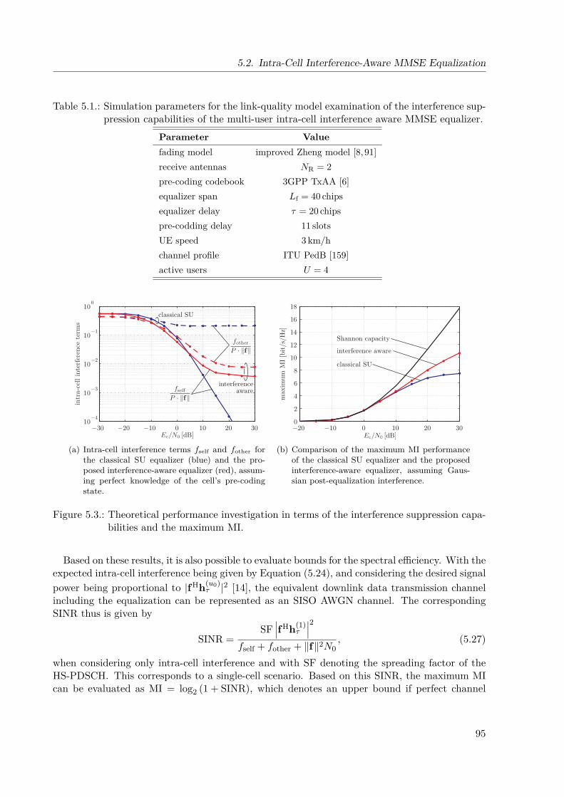
5.2. Intra-Cell Interference-Aware MMSE Equalization
Table 5.1.: Simulation parameters for the link-quality model examination of the interference sup-pression capabilities of the multi-user intra-cell interference aware MMSE equalizer.
Parameter Valuefading model improved Zheng model [8, 91]receive antennas NR = 2pre-coding codebook 3GPP TxAA [6]equalizer span Lf = 40 chipsequalizer delay τ = 20 chipspre-codding delay 11 slotsUE speed 3 km/hchannel profile ITU PedB [159]active users U = 4
−30 −20 −10 0 10 20 3010
−4
10−3
10−2
10−1
100
intr
a-ce
ll in
terf
eren
ce t
erm
s
interferenceaware
classical SU
(a) Intra-cell interference terms fself and fother forthe classical SU equalizer (blue) and the pro-posed interference-aware equalizer (red), assum-ing perfect knowledge of the cell’s pre-codingstate.
−20 −10 0 10 20 300
2
4
6
8
10
12
14
16
18
max
imum
MI
[bit/s
/Hz]
Shannon capacity
interference aware
classical SU
(b) Comparison of the maximum MI performanceof the classical SU equalizer and the proposedinterference-aware equalizer, assuming Gaus-sian post-equalization interference.
Figure 5.3.: Theoretical performance investigation in terms of the interference suppression capa-bilities and the maximum MI.
Based on these results, it is also possible to evaluate bounds for the spectral efficiency. With theexpected intra-cell interference being given by Equation (5.24), and considering the desired signalpower being proportional to |fHh(u0)
τ |2 [14], the equivalent downlink data transmission channelincluding the equalization can be represented as an SISO AWGN channel. The correspondingSINR thus is given by
SINR =SF∣∣∣fHh(1)
τ
∣∣∣2fself + fother + ‖f‖2N0
, (5.27)
when considering only intra-cell interference and with SF denoting the spreading factor of theHS-PDSCH. This corresponds to a single-cell scenario. Based on this SINR, the maximum MIcan be evaluated as MI = log2 (1 + SINR), which denotes an upper bound if perfect channel
95
Chapter 5. Multi-User MMSE Equalization for MIMO-Enhanced HSDPA
coding would by utilized. Note however, that this bound assumes a Gaussian distribution of thepost-equalization interference, which in practice is not necessarily the case. Nevertheless, the soderived maximum MI can serve as a figure of merit to assess the performance gain achievableby the interference-aware equalizer. Figure 5.3(b) shows the maximum MI for the classical SUequalizer and the interference-aware equalizer together with the Shannon channel capacity ofa NT × NR = 2 × 2 channel. It can be observed that the proposed equalizer offers significantpotential performance gains in the higher Ec/N0 region.
Moreover, in Appendix A.14 it is shown that under some coarse assumptions, the proposedinterference-aware equalizer maximizes the SINR in Equation (5.27). Thus, the equalizer is thebest linear filter for the intra-cell interference structure of the TxAA multi-user transmission.
5.2.2. Complexity
Given the solution of the intra-cell interference aware MMSE equalization in Equation (5.22), itis interesting to assess the additional complexity that is needed to compute the proposed filterwhen compared to the complexity of evaluating the classical SU equalizer.Assuming uncorrelatedtransmit sequences with constant power, thus implying Rxx = σ2
xI, the additional complexitycan be evaluated by looking at the product HwRxxHH
w ∝ HwHHw that is needed in the inverse
part of f in Equation (5.22). By writing
HwHHw = H
[W(MU)
(W(MU)
)H⊗ ILh+Lf−1
]HH, (5.28)
it can easily be seen that the additional cost of the proposed equalizer is only determined by thelarger matrix multiplication of W(MU)
(W(MU)
)Hinstead of W(SU)
(W(SU)
)H. In particular,
the complexities of these two operation can be approximated by
W(MU)(W(MU)
)H∼ O
(U + 2)3
, (5.29)
W(SU)(W(SU)
)H∼ O2 · 2 , (5.30)
if matrix multiplications are assumed to be of order Ok3, with k being the matrix dimension
for a square matrix. All the other matrix multiplications and the necessary inversion in Equa-tion (5.22) keep the same complexity, thus the additional complexity imposed by the intra-cell in-terference aware MMSE equalizer can be evaluated to be proportional to O
(U + 2)3 − 4
. The
complexity of the matrix inverse, however, can be approximated to be of order O
(NRLf)3
,and since U is typically much smaller than Lf in practical systems, the multiplication of themuti-user pre-coding matrix is negligible. Accordingly, the additional complexity needed for theconsideration of the pre-coding state of the cell is very moderate.
5.3. The Cell Pre-Coding State
In TxAA HSDPA, the MIMO channel is estimated by utilizing the CPICH, similar to UMTS.To be able to calculate the receive filter for the HS-DSCH data channel, however, the UE needsto know at least (i) the power offset of the individual HS-PDSCHs compared to the powerlevel of the CPICH, and (ii) the pre-coding coefficients that the base-station applied for the
96
5.3. The Cell Pre-Coding State
transmission.6 The power offset is signaled by higher layers [43], and the pre-coding coefficientsof all simultaneous transmissions are signaled on the according HS-SCCHs [35, 41], where everyactive user has his own channel. This unfortunately makes things difficult for the proposedequalizer, because the HS-SCCHs are scrambled with user-specific scrambling sequences,7 seealso Chapter 2, thus making it impossible to monitor the pre-coding state of the other usersactive in the cell.
In order to overcome this problem, one can think of three different strategies that are possible:
(i) change the signaling scheme in the HS-SCCH such that all active users know about thecomplete pre-coding state in the cell,
(ii) include some training data in the HS-PDSCHs of the users to be able to estimate thepre-coding state, or
(iii) blindly estimate the pre-coding state,
whereas (i) is an obvious solution that needs no further explanation. Thus, in the followingI will shortly discuss a possible solution for (ii), but the main focus will be dedicated to theblind estimation (iii) because it can be implemented without changes in the current transmissionstandard.8
The principal estimation problem is the following. According to Figure 5.1, every active usercan have his own pre-coding coefficient pair w(u)
1 , w(u)2 and his own power factor α(u), where
only the coefficients dedicated to the user himself are known. In addition, it is also not knownhow many users U are currently active. Estimation problems of this kind can be investigatedwithin the framework of random set theory [143], leading to optimum Bayesian ML estimators.However, these solutions require a joint estimation of the data-sequences of all users and thepre-coding state, which is typically very complex and thus disadvantageous for battery poweredmobile devices. Accordingly, I will restrict the efforts in this work onto classical approaches withmoderate complexity.
As explained in Appendix A.2, according to [6], the pre-coding codebook that is utilized inpractice is strongly quantized. In addition, several users may share the same pre-coding vector.Let me define the codebook of pre-coding vectors as
W ,v1, . . . ,v|W|
,w(u) ∈ W, (5.31)
with |W| specifies the cardinality of the codebook. Furthermore, let me denote the set of usersbeing served with the same pre-coding vector as Uk =
u : w(u) = vk
, with k = 1, . . . , |W|
denoting the codebook index of the corresponding pre-coding vector. Note that⋃|W|k=1 Uk does
not necessarily have to equal W, and that in case no user utilizes the pre-coding vector vk, thecorresponding set is empty Uk = ∅.
6This is due to the fact, that the channel estimation in UMTS and in HSDPA is based on the non pre-codedCPICH, see Chapter 4. Accordingly, at least the pre-coding coefficients for the desired user transmission areneeded to evaluate the MMSE equalizer weights for the classical SU equalizer.
7The scrambling sequence in HSDPA is a function of the user identification number, known only to the base-station and the particular user.
8This is an important argument for nearly all algorithmic improvements for current mobile communicationnetworks. A change in the standard would require huge efforts from both base-station and mobile-equipmentvendors, as well as from the 3GPP standardization body, which makes non standard-compliant improvementsnearly impossible to be implemented.
97
Chapter 5. Multi-User MMSE Equalization for MIMO-Enhanced HSDPA
Definition 5.1. The pre-coding state of an HSDPA cell is defined as
P ,α(1), . . . , α(k), . . . , α(|W|), α(p)
, (5.32)
where each α(k) denotes the power coefficient utilized to transmit on a particular pre-coding vectorw(k),
α(k) =√∑u∈Uk
(α(u))2. (5.33)
The coefficients α(u) denote the power coefficient of every user u = 1, . . . , U , as utilized inEquation (5.9).
With this definition, the two options for the pre-coding state estimation, (ii) training sequencesbased estimation, and (iii) blind estimation can be defined and their performance assessed.
5.3.1. Training-Sequence-based Pre-Coding State EstimationBefore going into the details on the training sequence based estimator, let me note that theinput-output relation in Equation (5.8) can be rewritten as
yi = H[XiD1XiD2
]α + ni, (5.34)
with the matrices D1 and D2 containing the pre-coding coefficients of the active users,
D1 = diagw
(1)1 , . . . , w
(U)1 , 1, 0
, (5.35)
D2 = diagw
(1)2 , . . . , w
(U)2 , 0, 1
, (5.36)
and the matrix Xi is the re-arranged transmit vector xi,
Xi =[x(1)i · · · x(U)
i p(1)i p(2)
i
]. (5.37)
Finally, the vector α lists the utilized power coefficients in the cell,
α =[α(1) · · · α(U) α(p) α(p)
]. (5.38)
Considering the special structure of the problem in Equations (5.8) and (5.34), some redun-dancy can be observed. In particular, if two users u1 and u2 utilize the same pre-coding vectorw(k), the input-output relation for these two users can also be represented by one combined useru′, utilizing w(k) with
α(u′) =√(
α(u1))2 +(α(u2))2 (5.39)
as his effective power coefficient. This is in concordance with the pre-coding state of the cell,as given in Definition 5.1. Furthermore, note that I assumed the non-data channels at the twotransmit antennas to deploy the same power coefficient α(p).
Given these arguments, it is sufficient to estimate only the pre-coding state P in order todescribe the whole pre-coding situation in the cell. For the interference-aware MMSE equalizeraccordingly the knowledge of P is sufficient to be able to suppress the intra-cell interferencecaused by the multi-user data transmission.
98
5.3. The Cell Pre-Coding State
Considering the definition of the pre-coding state P in Equation (5.32), the vector α =[α(1) · · · α(|W|) α(p)
]Thas to be estimated. Let me define the estimation error accordingly
asC =
∥∥∥α− ˆα∥∥∥2
2, (5.40)
with ˆα denoting the estimate of α. In case that training data is available, for example at thebeginning of each transmission frame in HSDPA, a possible estimator is given by the LS solution.The pre-coding codebook representing matrices can be set to
D1 , diagw
(1)1 , . . . , w
(|W|)1
, (5.41)
D1 , diagw
(1)2 , . . . , w
(|W|)2
. (5.42)
In addition, let me assume that the base-station provides orthogonal training sequences t(k) forevery pre-coding vector w(k), which can be formed into the training matrix
ST ,[t(1) · · · t(|W|)
]. (5.43)
Then the LS estimator of θ =[α(1) · · · α(|W|)
]T, not including α(p), is given by [92]
θLS = <
(
H[STD1STD2
])#
yi
+
, (5.44)
where the real-valued operator <·+ ensures that the coefficients are real valued and positive,even in the low SNR regime where the noise potentially causes non real-valued estimates. Thecoefficient α(p) can be calculated by utilizing the sum power constraint in Equation (5.10).Accordingly, the augmented LS estimate of α is given by
ˆαLS =[θT
LS 1− θTLSθLS
]T. (5.45)
5.3.2. Blind Pre-Coding State EstimationBlind estimation is in general a quite challenging task, in particular in the multi-user context.Typical approaches treat the unknown inputs—in this case the unknown transmit data yi—asnuisance parameters that the estimator has to cope with in order to supply blind estimates ofthe parameters of interest.
The ML principle provides a systematic way for deducing the Minimum Variance Unbiased(MVU) estimator, maximizing the joint likelihood function fy(y;α, x) [160]. As discussed in [161,162], there exist a number of possibilities to avoid the joint estimation of all parameters, inthis case α and xi. The unconditional or stochastic ML criterion models the vector of nuisanceparameters as a random vector and maximizes the marginal of the likelihood function conditionedto x,
fy(y;α) = Exfy|x(y|x;α)
, (5.46)
where Ex· stands for the expectation operator with respect to the transmit signal x.Unfortunately, the unconditional ML estimator is generally unknown, because the expectation
with respect to x typically cannot be solved in closed form. This is also the case for this
99
Chapter 5. Multi-User MMSE Equalization for MIMO-Enhanced HSDPA
particular problem. However, in the low SNR regime, the unconditional likelihood functionfy(y;α) becomes quadratic in the observation with independence of the statistical distributionof the nuisance parameters. This estimator class, however, is also generally difficult to solve andworks only reasonably well in the low SNR regime [160].
This fact motivated research in the area of second-order estimators, for example the conditionalML criterion that models the nuisance parameters as deterministic unknowns and maximizes thecompressed likelihood function fy
(y;α, ˆx
)in which ˆx denotes the ML estimate of x. Unfortu-
nately, for the particular problem of estimating the pre-coding state of the cell, this estimatorclass cannot be utilized because it would require the matrix Hw to be tall [162], which in theused signal model is not the case.
Another approach is the Gaussian ML estimator class which models the nuisance parametersas Gaussian random variables in order to obtain an analytical solution for the expectation inExfy|x(y|x;α)
[163]. This assumptions seems to fit naturally into the system-model because
due to multi-code operation many different transmit chips are added up, likely resulting in anear Gaussian distribution of the receive signal.9 Although there are also other approaches thatcould be utilized to blindly estimate α, for example [164], I decided in favor of this estimatorclass.
The Gaussian ML estimator for the pre-coding state of an HSDPA cell, is the one minimizingthe nonlinear cost function
ΛGML(α) = tr[ln R(α) + R−1(α) R
]= ln det [R(α)] + tr
[R−1(α) R
], (5.47)
with R = yiyHi denoting the sample covariance matrix, and
R(α) = HwHHw + σ2
nI (5.48)
being its expected value as a function of α. Note that I assumed Gaussian white noise withvariance σ2
n here.The direct application of this estimator would require the number of users U to be known for
the estimation, which is not the case in this problem setting. To overcome this problem, let mepoint out that W(MU) from Equation (5.9) can be rewritten as
W(MU) = W diagα, (5.49)
with W containing the same pre-coding coefficients as W(MU), but without the α(u) coefficients.Recalling that the goal is to estimate the pre-coding state P, the matrix W can be replaced inthe context of Equation (5.48) by
W =[w(1) · · · w(|W|)
]diag
[α(1) · · · α(|W|)
]T︸ ︷︷ ︸
θ
, (5.50)
thus leading toR(θ) = H
(WWH ⊗ I
)HH + σ2
nI, (5.51)
9For the interference power terms after equalization this assumption does not hold anymore, as shown in Chap-ter 3.
100
5.4. Performance Evaluation
and the new associated cost-function ΛGML(θ) = tr[ln R(θ) + R−1(θ) R
]. Please note that
as in the training based estimation, α(p) can be calculated from the sum power constraint inEquation (5.10).
The minimum of ΛGML can for example be found by means of iterative or time-recursivescoring methods [157,163], based on
θl+1 = θl + J−1GML
(θ)∇GML
(y; θ
), (5.52)
with J−1GML
(θ)
and ∇GML(y; θ
)being the Fisher information matrix and the gradient respec-
tively. Alternatively, any other known efficient optimization technique like for example Sequen-tial Quadratic Programming (SQP) methods [165] can be used. Such convex optimization basedtechniques potentially offer large complexity gains if the underlying problem shows some form ofsparsity which allows for a suitable factorization [156].
When utilizing the blind pre-coding state estimator, the overall complexity of the interferenceaware equalizer is of course increased. The computational complexity order of one step in theoptimization process can be approximated by the complexity of evaluating the cost function,which turns out to be proportional to
2[ONRLf (Lh + Lf − 1)2 (U + 2)NT
+O
(NRLf)2
+O
(NRLf)3
], (5.53)
where I again assumed a matrix multiplication complexity order of OK3. If an optimization
algorithm based on Newton iterations is utilized, the number of required iterations can alsocoarsely be bounded by log2 log2 1/ε with ε specifying the desired accuracy [156]. In practiceI observed a convergence of the utilized algorithm in around eight iterations. The blind pre-coding estimation thus increases the computational complexity much more significantly than thechanges in the MMSE equalizer structure.
5.3.3. Estimator PerformanceFigure 5.4 shows the Mean Squared Error (MSE) C of the two estimators for different Ec/N0values. The simulation parameters are the same as in Table 5.1, except that I simulated theperformance for one and two receive antennas, respectively. For the LS estimation, I usedHadamard sequences of length 64 for the training. To refine the estimation, I furthermoretook advantage of the knowledge that the coefficients α(k) have to be real valued and strictlypositive, as well as that the sum power constraint in Equation (5.10) cannot be exceeded. It canbe observed in Figure 5.4 that the training based estimator works reasonably well from -20 dBEc/N0 on, and that the performance saturates at around 10 dB. The blind estimator on the otherhand is not able to deliver similar results, and shows an operating range starting approximatelyat -10 dB Ec/N0. For both estimator classes, the availability of a second receive antenna isbeneficial for the pre-coding state estimation. However, for the blind pre-coding state estimatorthe gain is even more dramatic. Let me note that the (poor) performance of the blind estimatoris still sufficient for the proposed equalizer, as will be shown in the next section.
5.4. Performance EvaluationIn order to assess the performance of the proposed equalizer in comparison to the classical SUequalizer, as well as to evaluate the influence of the pre-coding state estimation, I split the
101

Chapter 5. Multi-User MMSE Equalization for MIMO-Enhanced HSDPA
−40 −30 −20 −10 0 10 2010
−5
10−4
10−3
10−2
10−1
100
blind estimation
training based
Figure 5.4.: Mean quadratic estimation error C—defined in Equation (5.40)—of the LS and thesecond-order blind pre-coding state estimators versus Ec/N0.
simulations into two different parts: (i) physical-layer simulations for a fixed transmission setupof TxAA HSDPA, and (ii) system-level simulations with adaptive feedback and scheduling. Eachsimulation approach has a different focus, with the physical-layer simulations covering channelencoding and decoding, WCDMA processing, as well as channel estimation in detail. On theother hand, system-level simulations represent a whole HSDPA network, with adaptive feedback,scheduling and RRC algorithms. For the following results I also assumed that the channel andthe noise power are perfectly known at the receiver.
5.4.1. Physical-Layer Simulation Results
I conducted physical-layer simulations utilizing a standard compliant WCDMA simulator [94].The simulation assumptions in Table 5.2 correspond to a cell in which four users are receivingdata simultaneously. User one is moving through the cell and obtains pre-coding coefficientsas adaptively requested, according to the definition in Appendix A.2 [6]. The three interferingusers are assumed to be stationary, thus their pre-coding coefficients and transmit power donot change. In the physical-layer simulations I furthermore assume that all users are alwaysscheduled with the same CQI value, thus no link adaptation besides the pre-coding takes place.
The achieved data throughput of user one in a PedA and PedB environment is plotted inFigures 5.5(a) and 5.5(b), respectively. In both scenarios, the interference-aware MMSE equalizerwith perfect knowledge of the pre-coding state significantly outperforms the SU MMSE equalizer.If the pre-coding state of the cell is blindly estimated, the performance of the MMSE equalizernearly approaches the performance when P is perfectly known.
The gain in the PedB channel in Figure 5.5(b) is much larger than the gain in the PedA channelwhich has a much shorter maximum delay spread. This is caused by the larger loss of orthog-onality in the PedB environment and the subsequently larger post-equalization interference. Inthe 2 × 1 case, the equalizer applying the blind pre-coding state estimation looses significantlycompared to the equalizer with perfect knowledge of P, which is a result of the considerablyworse estimator performance when only one receive antenna is available, see Figure 5.4. Thefact that the performance loss is greater in the PedB channel is due to its larger delay spread,which represents a more challenging environment for the equalizer making it more sensitive toestimation errors in the pre-coding state.
102

5.4. Performance Evaluation
Table 5.2.: Simulation parameters for the physical-layer simulation performance assessment ofthe interference-aware MMSE equalizer.Parameter Valueactive users U 4, capability class 6desired user CQI 13interfering HS-PDSCH Ec/Ior [−6,−8,−10] dBinterfering user CQIs [16, 11, 8]interfering user pre-coding [1, 1√
2 (1− j)], [1, 1√2 (−1 + j)], [1, 1√
2 (−1− j)]pre-coding codebook 3GPP TxAA [6]CPICH Ec/Ior −10 dBother non-data channel Ec/Ior −12 dBUE speed 3 km/h
−30 −25 −20 −15 −10 −50
0.2
0.4
0.6
0.8
1
1.2
thro
ughp
ut [M
bit/
s] IA blind
IA perfect
SU IA blind
IA perfect
SU
(a) Physical-layer throughput of the desired user ina spatially uncorrelated ITU PedA channel atCQI 13, corresponding to a maximum through-put of 1.14 Mbit/s.
−30 −25 −20 −15 −10 −50
0.2
0.4
0.6
0.8
1
1.2
thro
ughp
ut [M
bit/
s] IA blind
IA perfect
SU
IA blindIA perfect
SU
(b) Physical-layer throughput of the desired user ina spatially uncorrelated ITU PedB channel atCQI 13, corresponding to a maximum through-put of 1.14 Mbit/s.
Figure 5.5.: Physical-layer simulation results. The interference-aware equalizer is denoted IA.
For larger number of receive antennas, the simulation results show larger performance gains.Especially in Figure 5.5(b), the pre-coding state estimation becomes significantly better in the2× 2 case, thus closing the gap to the throughput performance of the equalizer utilizing perfectknowledge of P. The interference-aware MMSE equalizer can thus effectively utilize the spatialinformation to suppress the interfering signals. The largest performance increase of the proposedMMSE equalizer was found for the 2× 2 PedB environment with 4 dB.
5.4.2. System-Level Simulation Results
To assess the performance on network level, I also conducted a set of system-level simulationswith the simulator as described in Chapter 4 [13, 14]. The simulation assumptions in Table 5.3correspond to a 19 site scenario with a homogeneous network load in which the multi-codescheduler serves four active users simultaneously. All 25 simulated users are moving through the
103
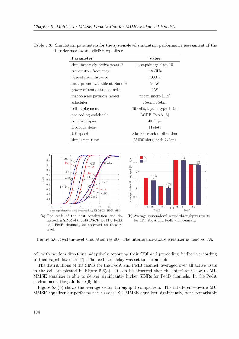
Chapter 5. Multi-User MMSE Equalization for MIMO-Enhanced HSDPA
Table 5.3.: Simulation parameters for the system-level simulation performance assessment of theinterference-aware MMSE equalizer.
Parameter Valuesimultaneously active users U 4, capability class 10transmitter frequency 1.9 GHzbase-station distance 1000 mtotal power available at Node-B 20 Wpower of non-data channels 2 Wmacro-scale pathloss model urban micro [112]scheduler Round Robincell deployment 19 cells, layout type I [93]pre-coding codebook 3GPP TxAA [6]equalizer span 40 chipsfeedback delay 11 slotsUE speed 3 km/h, random directionsimulation time 25 000 slots, each 2/3 ms
2 4 6 8 10 12 14 160
0.1
0.2
0.3
0.4
0.5
0.6
0.7
0.8
0.9
1
post equalization and despreading HSDSCH SINR [dB]
ecdf
SUIA SU
IA
IASU
IASUPedB
PedA
(a) The ecdfs of the post equalization and de-spreading SINR of the HS-DSCH for ITU PedAand PedB channels, as observed on networklevel.
0
0.5
1
1.5
2
2.5
3
aver
age
sect
or t
hrou
ghpu
t [M
bit/
s]
PedB PedA
IASU
11.7%
8,6%
1%
1%
(b) Average system-level sector throughput resultsfor ITU PedA and PedB environments.
Figure 5.6.: System-level simulation results. The interference-aware equalizer is denoted IA.
cell with random directions, adaptively reporting their CQI and pre-coding feedback accordingto their capability class [7]. The feedback delay was set to eleven slots.
The distributions of the SINR for the PedA and PedB channel, averaged over all active usersin the cell are plotted in Figure 5.6(a). It can be observed that the interference aware MUMMSE equalizer is able to deliver significantly higher SINRs for PedB channels. In the PedAenvironment, the gain is negligible.
Figure 5.6(b) shows the average sector throughput comparison. The interference-aware MUMMSE equalizer outperforms the classical SU MMSE equalizer significantly, with remarkable
104
5.5. Summary
gains in the PedB environment of up to 11.7 %. Similar to the physical-layer simulation results,for both channels the equalizer is able to utilize the advantage of multiple receive antennas,in this case the 2 × 2 MIMO channel, to advance the pre-coding state estimation. Thus, thethroughput performance is also higher than the one of the 2× 1 single antenna receiver case.
5.5. SummaryIn this chapter I proposed and investigated a MU interference-aware MMSE receiver with ablind cell pre-coding state estimator. The developed structure is an extension of the classical SUMMSE equalizer that takes the pre-coded intra-cell interference into account. This allows forachieving significant gains in the throughput performance.
Future research on this receiver would have to include a cancellation of the synchronizationchannel which has been shown to have a great impact on the performance [16]. Furthermore, theproposed interference-aware receiver only takes the intra-cell interference into account. However,for a close-to-optimum performance also the inter-cell interference should be mitigated. Thiswould require an even more detailed model representing the pre-coding of the neighboring cellsin a suitable way. Let me point out that also the proposed cell-pre-coding-state estimator offersroom for further research. By a closer investigation of the underlying blind estimation principle—maybe by a low-complexity approximation of a random set theory based approach—and carefuldesign of the utilized optimization algorithm, higher estimation accuracy as well as probably alower complexity might be achieved.
In the current state, the proposed receiver structure, however, offers a possibility to achievesignificant throughput gains in channels with larger delay spread by only moderately increasingthe computational complexity.
105

Chapter 6.
ConclusionsIn the end we retain from ourstudies only that which wepractically apply.
(Johann Wolfgang von Goethe)
Communication networks represent one of the driving forces behind the development of ourmodern information society. In particular, wireless networks have proven to enable many
data-driven services which we take for granted today.The wireless link, however, is affected by constraints on the available bandwidth, the max-
imum allowed transmission power, and deployment confinements of the necessary equipment.Accordingly, modern cellular networks have to exploit the given resources as efficient as possible,utilizing physical-layer processing techniques with high spectral efficiencies, but also optimizingnetwork-based multi-user algorithms.
Unfortunately, research in the field focuses strongly on the individual link, but often neglectsthe implications when the proposed techniques are employed in a multi-user, multi-base-stationcontext. Network-based algorithms can for example have a significant impact on the channelstatistics, but also other procedures like HARQ retransmissions, admission control, and resourceallocation protocols heavily affect the individual link. The upcoming network generations in-clude a MAC controlled physical-layer with potential cross-layer optimizations that have to beinvestigated taking the whole system into account.
System-level modeling and simulation provide such a possibility to investigate and assess manyof the requirements and performance implications of communication networks. The main con-tribution of this thesis thus is the development of a suitable system-model description of MIMOHSDPA networks and the subsequent application of this model to a set of optimizations, bothon the network as well as on the individual links.
Contributions of this Thesis
This thesis provides many insights and novel developments, both in the field of system-levelmodeling and in the optimization of the investigated MIMO HSDPA network.
The proposed link-quality model provides a very flexible and accurate analytical description ofthe MIMO HSDPA link-quality in the network context that was not available before. Utilizing anequivalent fading parameter structure the computational complexity of the model is vastly reducedcompared to a full physical-layer simulation and thus allows the simulation of large networks.Together with the proposed link-performance model which exploits slot-based sampling of thelink-quality parameters, a comprehensive system-level description of MIMO HSDPA networkswas created. The novel training method of the link-performance model furthermore allows for an
107
Chapter 6. Conclusions
increased accuracy in the BLER prediction. The flexibility and the accuracy of the model alsoled to its implementation in the Nokia Siemens Networks (NSN) system-level simulator MoRSE.
Based on the developed model, a flexible system-level simulator was programmed, suitablefor performance analysis and algorithm testing including the physical- and the MAC-layer. Thederived network performance prediction results are very valuable for network planning and in-vestment decisions. For the overall network performance, RLC algorithms play an crucial role.The developed RLC stream number decision algorithm is shown to be robust against UE CQIreporting inaccuracies, for example due to a small channel coherence time. It allows the networkoperator to allocate the MIMO resources and thus take control of the interference situation inthe cell. Similarly, the proposed content-aware MAC-hs scheduler is able to increase the QoEfor video-streaming services in HSDPA networks. The concept can also be applied to other ser-vices worth prioritizing. Moreover, this cross-layer scheduling approach strongly improves theflexibility compared to available algorithms operating in the physical-layer or in the MAC-layeronly.
This thesis also presents advances for the network operation. An HSDPA link-quality optimiz-ing CPICH power allocation is presented. It is shown that careful adjustment of the pilot powerimproves the operation of wireless cellular networks. Accordingly, the presented results are veryhelpful for MIMO HSDPA field trials or for the optimization of currently deployed HSDPA cellclusters.
As already mentioned, the individual link is also affected by the network behavior. In particu-lar, the interference structure has to be considered in order to derive optimum receiver structures.The proposed multi-user interference-aware MMSE equalizer offers large performance gain inchannels with larger delay spread. Such channels impose a low spreading code orthogonalitywhich can be regained with the proposed equalizer at only a moderately increased computa-tional complexity. The required blind pre-coding state estimator also opens ways for even moresophisticated exploitations of the knowledge about the interference structure in the cell.
Limits of the Work; Future Research
Despite the efforts and care taken during the work on the presented research topics, some remarksregarding the limitations have to be made. One of the most constricting assumptions in theproposed system-level model is that only linear receivers can be accurately represented. Thisexcludes for example SIC and ML based structures that have got more attention recently. Inorder to incorporate such receiver structures in the system-level model, significant changes inthe link-quality and in the link-performance model are necessary. Recent research has startedto investigate the implications of ML receivers on the link-performance model, but so far nocomplete system-level model is available.
Furthermore, another critical point is the behavior of the signaling channels and their modelingin the system-level simulator. Data transmission on the signaling channels is crucial for theoperation of any network, however, they are only roughly modeled at the moment. Additionally,in system-level simulations a separate model of the signaling channels would lead to a morerealistic representation of the influence on the overall network performance and the implicationson RLC algorithms. An accurate representation of the signaling is also advantageous for thedevelopment of network equipment.
The proposed model would also benefit from a more detailed investigation of the Doppler effectand its influence on the equivalent fading parameters and the requirements for the slot-basedsampling in the link-performance model. It has to be noted, though, that HSDPA is mainly used
108

in static scenarios which is already well covered by the presented model. Nevertheless, futuregeneration networks may very likely provide service in high-speed transportation like trains.
Finally, I would like to point out that validation is a crucial point in the design of a system-level model. Exhaustive validation of this very complex system-level simulator is impossible,however, standardized test-scenarios that can be simulated in a link-level and a system-levelsimulator would simplify matters. For MIMO HSDPA this unfortunately was not possible dueto the restrictions of the utilized link-level simulator. However, these ideas will be included inthe system-level research on LTE in which I am currently involved [166,167].
Lessons Learned
The research and work conducted in this thesis were very interesting and challenging and led meto a number of insights:
• A structured approach for the research and the necessary programming work is crucial fortimely progress. Nowadays, no researcher works on his own but rather is part of a teamof colleagues all over the world. Only when the research activities are well structured anddocumented right from the start, the full potential of collaborations can be exploited.• The success of a model is not only determined by its scientific appeal and accuracy, but
also by its simplicity. Models are not only used by their designer but also by many others.Thus simpler models are much easier to explain and understand, and consequently theiracceptance in the scientific community is usually larger. However—as Albert Einsteinalready pointed out—one should not forget the following:
“Make everything as simple as possible, but not simpler.”• Validation is the foundation of scientific research. Without meaningful ways of validation,
even the best model cannot prove its value. How can one otherwise be sure that one ismodeling what one wants to model? Accordingly, means for validation should be kept inmind already during the design of the model to allow for efficient testing.• Modern wireless communication systems do not allow for an individual treatment of the
involved layers anymore. The merging of the lower layers allows cross-layer optimization,but on the other hand makes a separate design of every layer impossible. This, however, re-quires a much broader understanding of the whole network, which is particularly importantto be able to conduct system-level research.
Will we need System-Level Research in the Future?
With growing intelligence of the physical-layer nodes, LTE shifts the RNC algorithms into theeNodeBs and enables inter-NodeB communication. This opens a number of possibilities fornetwork optimization and requires detailed investigation of algorithms on large cellular networkscale. Without ways to test and predict the functionality of those new algorithms, no meaningfulperformance comparison can be made. Accordingly, system-level research will even become moreimportant for the next generations of wireless networks.
109

Appendix A.
Additional MaterialInformation is a source of learning.But unless it is organized, processed,and available to the right people ina format for decision making, it is aburden, not a benefit.
(William Pollard)
My intention when writing this thesis was to keep the main chapters as precise and struc-tured as possible, thus some of the related information that would have disturbed and/or
complicated the reading have been left out on purpose. Some of the details given here howeverare needed for arranging and conducting the simulations, respectively the understanding of someimplementation specific conclusions. Thus I include short discussions about the relevant pointsin this appendix.
A.1. Standardization, Current Deployment of HSDPA
The 3GPP is the forum where standardization has been handled from the first WCDMA UMTSspecification on. It unites many telecommunication standard bodies to coordinate their regionalactivities in order to establish global standards aligned down to bit level details. The 3GPPwas created in December 1998, with the original scope of producing technical specifications andtechnical reports for 3G mobile systems, both for FDD and TDD modes, respectively. The scopewas subsequently amended to include the maintenance and development of GSM, General PacketRadio Service (GPRS) and Enhanced Data Rates for Global system for mobile communicationsEvolution (EDGE) specifications. The specifications themselves are published regularly, withmajor milestones being denoted as Releases [168].
Figure A.1 shows the chronological development of the 3GPP standardization releases. Duringthe work on Release 4, it became obvious that some improvements for packet access would beneeded [33]. Release 5, which was finished in June 2002 thus introduced a high-speed enhance-ment for the downlink packet data services, HSDPA. The innovation that happened for HSDPAwas quite tremendous, including changes in the physical layer, the MAC layer and slight changesin the core network. After some years, to be specific in March 2005, 3GPP finished its work onRelease 6, specifying the uplink pendant of HSDPA, called HSUPA.
MIMO has been of interest already during the work on Release 5 and Release 6, however thefeasibility studies up to that point concluded that the benefits of it were limited to the extendthat the additional complexity could not be justified. Finally, after a long and detailed study-work discussing many proposals [6], MIMO has been included in Release 7 in December 2007.Besides this revolutionary step, the 3GPP added also many other improvements, among which
111
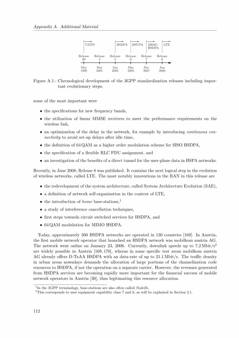
Appendix A. Additional Material
Mar1999
Mar2001
Jun2002
Mar2005
Dec2007
Jun2008
Release99
Release4
Release5
Release6
Release7
Release8
UMTS HSDPA HSUPA MIMOHSDPA
LTE
Figure A.1.: Chronological development of the 3GPP standardization releases including impor-tant evolutionary steps.
some of the most important were
• the specifications for new frequency bands,
• the utilization of linear MMSE receivers to meet the performance requirements on thewireless link,
• an optimization of the delay in the network, for example by introducing continuous con-nectivity to avoid set-up delays after idle time,
• the definition of 64 QAM as a higher order modulation scheme for SISO HSDPA,
• the specification of a flexible RLC PDU assignment, and
• an investigation of the benefits of a direct tunnel for the user-plane data in HSPA networks.
Recently, in June 2008, Release 8 was published. It contains the next logical step in the evolutionof wireless networks, called LTE. The most notably innovations in the RAN in this release are
• the redevelopment of the system architecture, called System Architecture Evolution (SAE),
• a definition of network self-organization in the context of LTE,
• the introduction of home base-stations,1
• a study of interference cancellation techniques,
• first steps towards circuit switched services for HSDPA, and
• 64 QAM modulation for MIMO HSDPA.
Today, approximately 300 HSDPA networks are operated in 130 countries [169]. In Austria,the first mobile network operator that launched an HSDPA network was mobilkom austria AG.The network went online on January 23, 2006. Currently, downlink speeds up to 7.2 Mbit/s2
are widely possible in Austria [169, 170], wheras in some specific test areas mobilkom austriaAG already offers D-TxAA HSDPA with an data-rate of up to 21.1 Mbit/s. The traffic densityin urban areas nowadays demands the allocation of large portions of the channelization coderesources to HSDPA, if not the operation on a separate carrier. However, the revenues generatedfrom HSDPA services are becoming rapidly more important for the financial success of mobilenetwork operators in Austria [30], thus legitimating this resource allocation.
1In the 3GPP terminology, base-stations are also often called NodeBs.2This corresponds to user equipment capability class 7 and 8, as will be explained in Section 2.1.
112
A.2. Pre-Coding Codebook; Pre-Coding Evaluation
A.2. Pre-Coding Codebook; Pre-Coding Evaluation
The 3GPP technical recommendation [6] specifies a pre-coding codebook for D-TxAA MIMOHSDPA. The pre-coding coefficients for the double-stream operation, are defined as
w1 = w3 ,1√2, (A.1)
w2 ∈1 + j
2 ,1− j
2 ,−1 + j
2 ,−1− j
2
, (A.2)
w4 , −w2, (A.3)
where w1 and w2 are utilized by stream one, and w3 and w4 are utilized by stream two. Accord-ingly the pre-coding matrix WCB would be given by
WCB =[w1 w3w2 w4
]=[w1 w2
]= WCB(w2) , (A.4)
which is fully determined by the choice of the pre-coding weight w2 in this case. It also has to benoted that, given the pre-coding weights of Equations (A.1) to (A.3), the pre-coding matrix isunitary, thus fulfilling the assumption in Theorem 3.1, in case of a double-stream transmission.For the single-stream transmission, only the pre-coding vector w1 is utilized.
With this definition of the pre-coding codebook, it remains to elaborate how the best pre-coding choice can be determined by the UE. First, it is necessary to define a metric in orderto be able to introduce a measure for the term best. For this purpose, many different figuresof merit could be used, like for example the capacity, achievable maximum rate, or the BLERperformance.
The question of the metric to be optimized for the pre-coding in MIMO systems as well asthe algorithm solving for the metric has been investigated by researches in great detail. Manyapproaches have been proposed, for example based on interference alignment ideas [171], utilizinggame-theoretic concepts [172], introducing the energy efficiency into the problem [173], takinginto account that the channel is only imperfectly known [174], applying DPC3 techniques [176],aiming for robust solutions [177], or trying to exploit the benefits of joint pre-coding and schedul-ing [178]. A lot of research has also tried to include coordination among the transmitters, thatis the NodeBs, in the problem. In HSDPA, such approaches are currently not supported bythe network, however, in LTE the X2-interface will provide means to allow for such algorithms.Despite all these research efforts, the 3GPP recommends the utilization of the SINR as the un-derlying metric to decide upon the pre-coding vector choice [6, 7]. Only a coordination with thescheduler regarding the pre-coding utilization would be possible.
Defining the SINR as the cost function to be maximized, it is still unclear, which SINR shouldbe considered. Given the structure of MIMO HSDPA, see also Figure 2.8, the SINR metric canbe evaluated
• before the equalization, thus directly at the receive antennas, or• after the equalization, which is much more complex to be evaluated.4
3DPC is a technique for pre-destorting the transmit signal to cancel the interference at the receiver end [175].4Note that the post-equalization SINR builds the basis for the system-level model in Chapter 3 with the de-
spreading gain included.
113
Appendix A. Additional Material
For the UE to utilize the post-equalization SINR as a decision metric for the pre-coding, thereceive filter would have to be evaluated for all—or at least a set of—pre-coding possibilities.Given the limited computational power and battery constraints in wireless mobile devices, suchcalculations are intractable. For sake of completeness, I want to point out that there may bepossibilities to assess the post-equalization SINR as a metric by a suitable low-complex repre-sentation. If done so, this also allows for the possibility of joint pre-coding and link-adaptationfeedback reporting [16]. Moreover, I will not consider this possibility in this work.
Due to its anticipated lower computational complexity, I consider the case of the pre-equaliza-tion SINR metric for this work. Considering Equation (3.6), the samples at receive antenna nrare given by
y(nr)i = h(nr)
w xi + ni, (A.5)
where h(nr)w , (Hw)(nr,:) is defined to be the nr-th row of the equivalent MIMO channel matrix
Hw, defined in Equation (3.2). Considering that there are multiple streams transmitted to thereceiver, the above equation can be rewritten as
y(nr)i =
NS∑n=1
h(nr,n)w x(n)
i + ni, (A.6)
where h(nr,n)w is composed of the columns with indices5 n+NS[1, Lh] from the vector h(nr)
w . Thechannel vector entries of h(nr,n)
w correspond to the transmit chips of stream n, and correspond-ingly, x(n)
i is defined to contain only the transmit chips of that respective stream. With thesedefinitions, the pre-equalization SINR of stream n on receive antenna nr is given by
ρ(n,nr) =E∣∣∣h(nr,n)
w x(n)i
∣∣∣2E∑NS
m=1m 6=n
∣∣∣h(nr,m)w x(m)
i
∣∣∣2+ E|ni|2
. (A.7)
For simplifying this equation, consider
E∣∣∣h(nr,n)
w x(n)i
∣∣∣2 = h(nr,n)w E
x(n)i
(x(n)i
)H(
h(nr,n)w
)H= h(nr,n)
w
(h(nr,n)
w
)H, (A.8)
where I assumed the data chips to be i.i.d. uncorrelated with unit variance, Ec = 1. Note alsothat the stream-specific equivalent MIMO channel row h(nr,n)
w is equal to
h(nr,n)w = H(nr,:) (I⊗wn) = wH
n
(H(nr)
)HH(nr)wn, (A.9)
according to Equation (3.2), and with H(nr) defining the CLh×NT frequency selective MIMO chan-nel matrix that contains the channel coefficients from all transmit antennas to receive antennanr. Accordingly, Equation (A.7) becomes
ρ(n,nr) =wHn
(H(nr)
)HH(nr)wn∑NS
m=1m6=n
wHm
(H(nr))H H(nr)wm + σ2
n, (A.10)
5I utilize the notation [a, b] do denote all integers between a and b, for example [3, 9] = 3, 4, . . . , 9.
114
A.2. Pre-Coding Codebook; Pre-Coding Evaluation
with σ2n defining the variance of the i.i.d. white Gaussian noise.
The UE thus has to find the optimum pre-coding vector for each stream by solving the SINRrelated problem
WoptCB = arg max
WCB
NS∑n=1
NR∑nr=1
ρ(n,nr), (A.11)
which optimizes the sum SINR over all receive antennas and streams. This is a particularlydifficult problem to solve, in particular because—like in the 3GPP pre-coding codebook—the pre-coding vectors can have dependencies, thus the problem in Equation (A.11) cannot be decoupledfor the individual streams.
Accordingly, a low complexity approach would be to optimize
woptn = arg max
wn
NR∑nr=1
wHn
(H(nr)
)HH(nr)wn = arg max
wnwHn
NR∑nr=1
(H(nr)
)HH(nr)
︸ ︷︷ ︸
,R
wn (A.12)
instead of Equation (A.11), for each stream individually. In the D-TxAA MIMO HSDPA case,only one stream has to be evaluated, because the second stream is directly specified by thecodebook, given in Equations (A.1) to (A.3). Thus, in this work, the pre-coding was chosenaccording to the optimization over the pre-coding weight w2,
wopt2 = arg max
w2wH
1 Rw1, (A.13)
which of course favors stream one, thus explaining for example the gap between the ecdfs of theequivalent fading parameters in Figure 3.5.
To overcome the problem of favoring stream one, the optimization problem could be alteredto
wopt2 = arg max
w2wH
1 Rw1 + wH2 Rw2, (A.14)
thus searching for the best combination of the two pre-coding vectors.In order to assess the performance of the optimization in Equation (A.13) and ??, I conducted a
simulation comparing them with the optimum pre-coding vector choices, given by the eigenvectorscorresponding to the largest eigenvalues of R,6
woptn = un, un , U(:,n) : R = UΛU−1, (A.15)
with U and Λ denoting the unitary matrix of eigenvectors and the matrix of eigenvalues, bothsorted according to the magnitude of the eigenvalue. The simulation parameters for the simula-tion are given in Table A.1. The chip level SINR was chosen to be Ec/N0 = 0 dB, which impliesthat σ2
n = 1.The simulation results are given in Figure A.2, showing the sum SINR over all streams and
receive antennas,∑NSn=1
∑NRnr=1 ρ
(n,nr). It can be observed that both algorithms loose compared tothe non-quantized pre-coding choice from Equation (A.15). Interestingly, the algorithm greedilyaiming for the optimization of stream one from Equation (A.13) outperforms the algorithmconsidering both streams in Equation (A.14). This is due to the fact that both algorithmsare only an approximation to the problem in Equation (A.11). These results also proof theapplicability of the algorithm utilized for the simulations in this thesis.
6Note that R is a Hermitian positive semi-definite square matrix, thus Singular Value Decomposition (SVD) andeigenvalue decomposition deliver equal results.
115
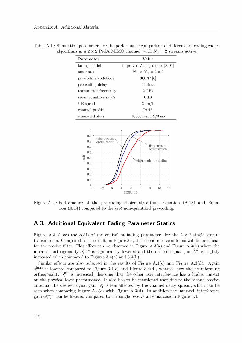
Appendix A. Additional Material
Table A.1.: Simulation parameters for the performance comparison of different pre-coding choicealgorithms in a 2× 2 PedA MIMO channel, with NS = 2 streams active.
Parameter Valuefading model improved Zheng model [8, 91]antennas NT ×NR = 2× 2pre-coding codebook 3GPP [6]pre-coding delay 11 slotstransmitter frequency 2 GHzmean equalizer Ec/N0 0 dBUE speed 3 km/hchannel profile PedAsimulated slots 10000, each 2/3 ms
−4 −2 0 2 4 6 8 10 120
0.1
0.2
0.3
0.4
0.5
0.6
0.7
0.8
0.9
1
SINR [dB]
ecdf
first streamoptimization
joint streamoptimization
eigenmode pre-coding
Figure A.2.: Performance of the pre-coding choice algorithms Equation (A.13) and Equa-tion (A.14) compared to the best non-quantized pre-coding.
A.3. Additional Equivalent Fading Parameter Statics
Figure A.3 shows the ecdfs of the equivalent fading parameters for the 2 × 2 single streamtransmission. Compared to the results in Figure 3.4, the second receive antenna will be beneficialfor the receive filter. This effect can be observed in Figure A.3(a) and Figure A.3(b) where theintra-cell orthogonality ointra
1 is significantly lowered and the desired signal gain Gs1 is slightly
increased when compared to Figures 3.4(a) and 3.4(b).Similar effects are also reflected in the results of Figure A.3(c) and Figure A.3(d). Again
ointra1 is lowered compared to Figure 3.4(c) and Figure 3.4(d), whereas now the beamforming
orthogonality oBF1 is increased, denoting that the other user interference has a higher impact
on the physical-layer performance. It also has to be mentioned that due to the second receiveantenna, the desired signal gain Gs
1 is less affected by the channel delay spread, which can beseen when comparing Figure A.3(c) with Figure A.3(d). In addition the inter-cell interferencegain Ginter
1,b can be lowered compared to the single receive antenna case in Figure 3.4.
116
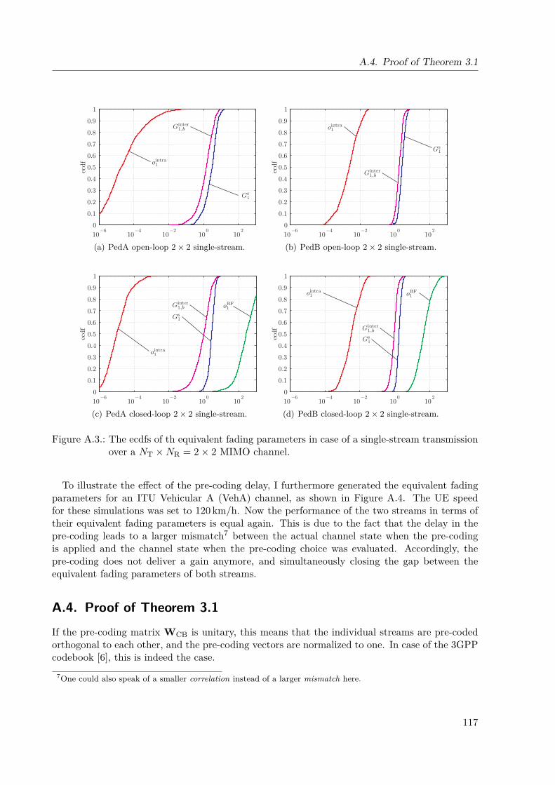
A.4. Proof of Theorem 3.1
10−6
10−4
10−2
100
102
0
0.1
0.2
0.3
0.4
0.5
0.6
0.7
0.8
0.9
1
ecdf
(a) PedA open-loop 2× 2 single-stream.10
−610
−410
−210
010
20
0.1
0.2
0.3
0.4
0.5
0.6
0.7
0.8
0.9
1
ecdf
(b) PedB open-loop 2× 2 single-stream.
10−6
10−4
10−2
100
102
0
0.1
0.2
0.3
0.4
0.5
0.6
0.7
0.8
0.9
1
ecdf
(c) PedA closed-loop 2× 2 single-stream.10
−610
−410
−210
010
20
0.1
0.2
0.3
0.4
0.5
0.6
0.7
0.8
0.9
1ecdf
(d) PedB closed-loop 2× 2 single-stream.
Figure A.3.: The ecdfs of th equivalent fading parameters in case of a single-stream transmissionover a NT ×NR = 2× 2 MIMO channel.
To illustrate the effect of the pre-coding delay, I furthermore generated the equivalent fadingparameters for an ITU Vehicular A (VehA) channel, as shown in Figure A.4. The UE speedfor these simulations was set to 120 km/h. Now the performance of the two streams in terms oftheir equivalent fading parameters is equal again. This is due to the fact that the delay in thepre-coding leads to a larger mismatch7 between the actual channel state when the pre-codingis applied and the channel state when the pre-coding choice was evaluated. Accordingly, thepre-coding does not deliver a gain anymore, and simultaneously closing the gap between theequivalent fading parameters of both streams.
A.4. Proof of Theorem 3.1
If the pre-coding matrix WCB is unitary, this means that the individual streams are pre-codedorthogonal to each other, and the pre-coding vectors are normalized to one. In case of the 3GPPcodebook [6], this is indeed the case.
7One could also speak of a smaller correlation instead of a larger mismatch here.
117
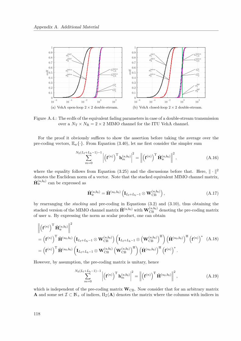
Appendix A. Additional Material
10−6
10−4
10−2
100
102
0
0.1
0.2
0.3
0.4
0.5
0.6
0.7
0.8
0.9
1ecdf
(a) VehA open-loop 2× 2 double-stream.10
−610
−410
−210
010
20
0.1
0.2
0.3
0.4
0.5
0.6
0.7
0.8
0.9
1
ecdf
(b) VehA closed-loop 2× 2 double-stream.
Figure A.4.: The ecdfs of the equivalent fading parameters in case of a double-stream transmissionover a NT ×NR = 2× 2 MIMO channel for the ITU VehA channel.
For the proof it obviously suffices to show the assertion before taking the average over thepre-coding vectors, Ew·. From Equation (3.40), let me first consider the simpler sum
NS(Lf+Lh−1)−1∑m=0
∣∣∣∣(f (n))T
h(u,b0)m
∣∣∣∣2 =∥∥∥∥(f (n)
)TH(u,b0)
w
∥∥∥∥2, (A.16)
where the equality follows from Equation (3.25) and the discussions before that. Here, ‖ · ‖2denotes the Euclidean norm of a vector. Note that the stacked equivalent MIMO channel matrix,H(u,b0)
w can be expressed as
H(u,b0)w = H(u0,b0)
(ILf+Lh−1 ⊗W(u,b0)
CB
), (A.17)
by rearranging the stacking and pre-coding in Equations (3.2) and (3.10), thus obtaining thestacked version of the MIMO channel matrix H(u,b0) with W(u,b0)
CB denoting the pre-coding matrixof user u. By expressing the norm as scalar product, one can obtain∥∥∥∥(f (n)
)TH(u,b0)
w
∥∥∥∥2
=(f (n)
)TH(u0,b0)
(ILf+Lh−1 ⊗W(u,b0)
CB
)(ILf+Lh−1 ⊗
(W(u,b0)
CB
)H)(
H(u0,b0))H (
f (n))∗
=(f (n)
)TH(u0,b0)
(ILf+Lh−1 ⊗W(u,b0)
CB
(W(u,b0)
CB
)H)(
H(u0,b0))H (
f (n))∗.
(A.18)
However, by assumption, the pre-coding matrix is unitary, hence
NS(Lf+Lh−1)−1∑m=0
∣∣∣∣(f (n))T
h(u,b0)m
∣∣∣∣2 =∥∥∥∥(f (n)
)TH(u0,b0)
∥∥∥∥2, (A.19)
which is independent of the pre-coding matrix WCB. Now consider that for an arbitrary matrixA and some set I ⊂ N+ of indices, ΠI(A) denotes the matrix where the columns with indices in
118
A.5. Further Link-Quality Model Validation Results
I are deleted. For the particular index set [τNS, τNS +NS − 1] it can be shown rather quicklythat
Π[τNS,τNS+NS−1](H(u,b0)
w
)= Π[τNT,τNT+NT−1]
(H(u0,b0)
)·(ILf+Lh−2 ⊗W(u,b0)
CB
), (A.20)
which implies that the operator ΠI preserves the structure of the matrix H(u,b0)w . Hence, using
the arguments from above,
NS(Lf+Lh−1)−1∑m=0
m6=[τNS,τNS+NS−1]
∣∣∣∣(f (n))T
h(u,b0)m
∣∣∣∣2 =∥∥∥∥(f (n)
)TΠ[τNS,τNS+NS−1]
(H(u,b0)
w
)∥∥∥∥2
=∥∥∥∥(f (n)
)TΠ[τNT,τNT+NT−1]
(H(u0,b0)
)∥∥∥∥2.
(A.21)
This is again independent of the user index u, and exactly equal to γ−1s in Equation (3.40), thus
concluding the proof.
A.5. Further Link-Quality Model Validation ResultsFigure A.5 shows the validation results for an equalizer span of Lf = 30 chips. The principalconclusions stay the same, however, compared to Figure 3.7, the saturation of the HS-PDSCHSINR in case of the PedB channel profile is less prominent. The reason for this is that with alarger equalizer span, the receive filter has more DoF to restore the orthogonality, thus leadingto a performance more close to the PedA channel with much smaller delay spread than the PedBchannel.
Figure A.6 depicts the results for the VehA channel, when the UE speed is set to 120 km/h.It can be observed that the performance of the SISO 1 × 1 mode and the MISO 2 × 1 modebecome equal, thus the second transmit antenna cannot be exploited to the extend as in lowspeed scenarios. This is due to the fact that the applied pre-coding is based on outdated channelinformation, because of the feedback delay, which was already mentioned in Section 3.3.4. Thesame argument holds for the diminishing performance gap between stream one and stream twoin case of the MIMO 2 × 2 DS mode. However, note that in context of these high UE speedsand according Doppler frequencies as well as small channel coherence time, the applicability ofthe block-fading assumption is more than questionable. Since the utilized fading simulator isbuilt on this assumption, no inter-symbol interference is taken into account, which limits thesignificance of the validation in Figure A.6.
A.6. Discussion of Assumption 3.9To generate the equivalent fading parameter of the inter-cell interference, there are basically twopossibilities to guarantee that the pre-coding choices of the neighboring cells are independentof the user channel. It can (i) either be assumed that the neighboring cell utilizes a randompre-coding, or (ii) that the pre-coding is static, that means constant over time. Alternative(i) guarantees a good averaging over different interference situations, however, the pre-codingchoices are not correlated over time. On the other hand, alternative (ii) represents a worst casescenario.
In order to decide which one of the two alternatives to use, I performed two sets of simulations:
119
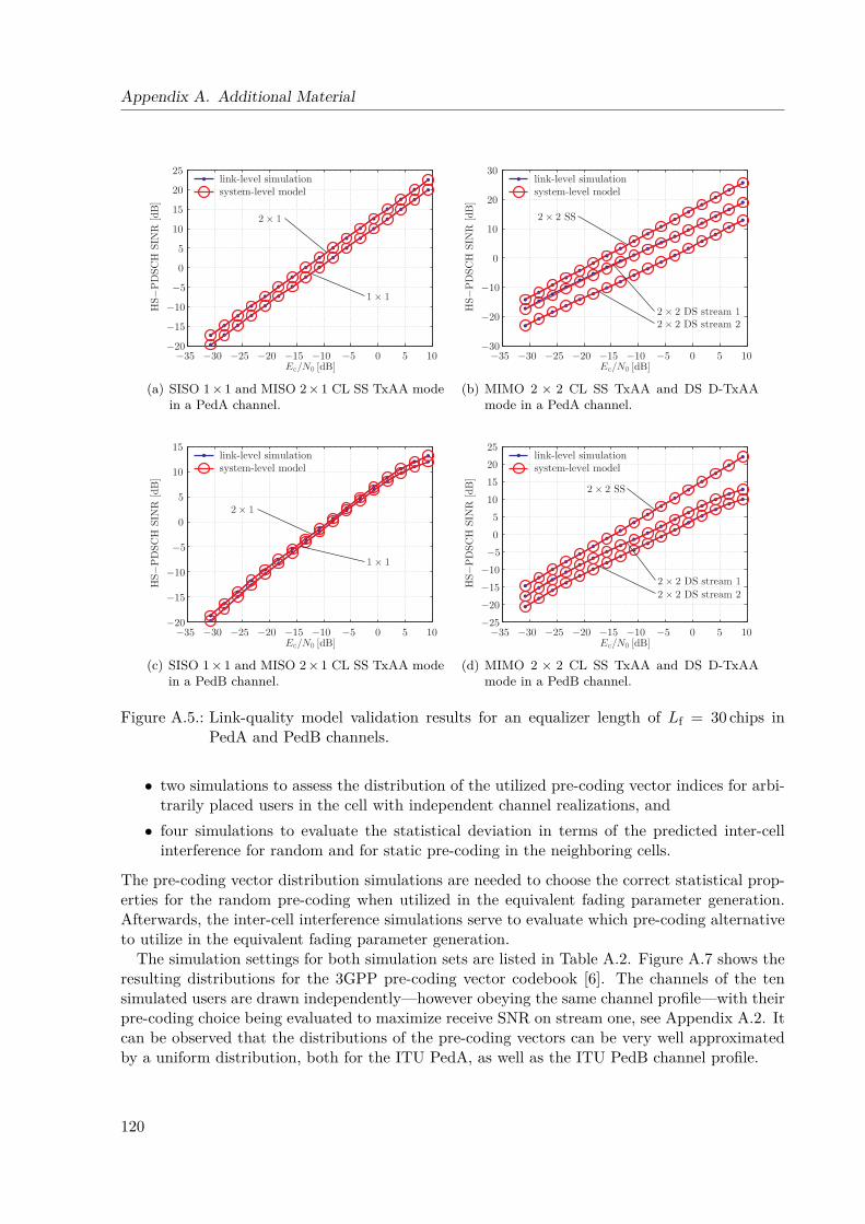
Appendix A. Additional Material
−35 −30 −25 −20 −15 −10 −5 0 5 10−20
−15
−10
−5
0
5
10
15
20
25
HS−
PD
SCH
SIN
R [dB
]
link-level simulationsystem-level model
(a) SISO 1× 1 and MISO 2× 1 CL SS TxAA modein a PedA channel.
−35 −30 −25 −20 −15 −10 −5 0 5 10−30
−20
−10
0
10
20
30
HS−
PD
SCH
SIN
R [dB
]
link-level simulationsystem-level model
(b) MIMO 2 × 2 CL SS TxAA and DS D-TxAAmode in a PedA channel.
−35 −30 −25 −20 −15 −10 −5 0 5 10−20
−15
−10
−5
0
5
10
15
HS−
PD
SCH
SIN
R [dB
]
link-level simulationsystem-level model
(c) SISO 1× 1 and MISO 2× 1 CL SS TxAA modein a PedB channel.
−35 −30 −25 −20 −15 −10 −5 0 5 10−25
−20
−15
−10
−5
0
5
10
15
20
25
HS−
PD
SCH
SIN
R [dB
]link-level simulationsystem-level model
(d) MIMO 2 × 2 CL SS TxAA and DS D-TxAAmode in a PedB channel.
Figure A.5.: Link-quality model validation results for an equalizer length of Lf = 30 chips inPedA and PedB channels.
• two simulations to assess the distribution of the utilized pre-coding vector indices for arbi-trarily placed users in the cell with independent channel realizations, and• four simulations to evaluate the statistical deviation in terms of the predicted inter-cell
interference for random and for static pre-coding in the neighboring cells.
The pre-coding vector distribution simulations are needed to choose the correct statistical prop-erties for the random pre-coding when utilized in the equivalent fading parameter generation.Afterwards, the inter-cell interference simulations serve to evaluate which pre-coding alternativeto utilize in the equivalent fading parameter generation.
The simulation settings for both simulation sets are listed in Table A.2. Figure A.7 shows theresulting distributions for the 3GPP pre-coding vector codebook [6]. The channels of the tensimulated users are drawn independently—however obeying the same channel profile—with theirpre-coding choice being evaluated to maximize receive SNR on stream one, see Appendix A.2. Itcan be observed that the distributions of the pre-coding vectors can be very well approximatedby a uniform distribution, both for the ITU PedA, as well as the ITU PedB channel profile.
120
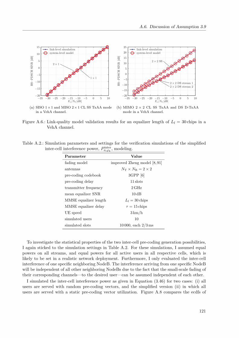
A.6. Discussion of Assumption 3.9
−35 −30 −25 −20 −15 −10 −5 0 5 10−20
−15
−10
−5
0
5
10
15
HS−
PD
SCH
SIN
R [dB
]
link-level simulationsystem-level model
(a) SISO 1× 1 and MISO 2× 1 CL SS TxAA modein a VehA channel.
−35 −30 −25 −20 −15 −10 −5 0 5 10−20
−15
−10
−5
0
5
10
15
20
25
HS−
PD
SCH
SIN
R [dB
]
link-level simulationsystem-level model
(b) MIMO 2 × 2 CL SS TxAA and DS D-TxAAmode in a VehA channel.
Figure A.6.: Link-quality model validation results for an equalizer length of Lf = 30 chips in aVehA channel.
Table A.2.: Simulation parameters and settings for the verification simulations of the simplifiedinter-cell interference power, P inter
n,ϕk, modeling.
Parameter Valuefading model improved Zheng model [8, 91]antennas NT ×NR = 2× 2pre-coding codebook 3GPP [6]pre-coding delay 11 slotstransmitter frequency 2 GHzmean equalizer SNR 10 dBMMSE equalizer length Lf = 30 chipsMMSE equalizer delay τ = 15 chipsUE speed 3 km/hsimulated users 10simulated slots 10 000, each 2/3 ms
To investigate the statistical properties of the two inter-cell pre-coding generation possibilities,I again sticked to the simulation settings in Table A.2. For these simulations, I assumed equalpowers on all streams, and equal powers for all active users in all respective cells, which islikely to be set in a realistic network deployment. Furthermore, I only evaluated the inter-cellinterference of one specific neighboring NodeB. The interference arriving from one specific NodeBwill be independent of all other neighboring NodeBs due to the fact that the small-scale fading oftheir corresponding channels—to the desired user—can be assumed independent of each other.
I simulated the inter-cell interference power as given in Equation (3.46) for two cases: (i) allusers are served with random pre-coding vectors, and the simplified version (ii) in which allusers are served with a static pre-coding vector utilization. Figure A.8 compares the ecdfs of
121

Appendix A. Additional Material
1 2 3 40
0.05
0.1
0.15
0.2
0.25
0.3
0.35
pre−coding vector index
epdf
(a) Pre-coding vector distribution in an ITU PedAchannel.
1 2 3 40
0.05
0.1
0.15
0.2
0.25
0.3
0.35
pre−coding vector index
epdf
(b) Pre-coding vector distribution in an ITU PedBchannel.
Figure A.7.: Pre-coding vector distribution in a NT×NR = 2×2 MIMO channel for two differentchannel profiles.
the inter-cell interference in Equation (3.46), normalized to the total power after the receivefilter, for different channel types and stream numbers in a Release 7 D-TxAA HSDPA system.The random pre-coding is chosen with a uniform distribution of the pre-coding vectors in thecodebook Ω. Note that the MIMO channel matrix for is normalized to an average power of one,that is E
‖Hw‖fro
= 1, with ‖ · ‖fro denoting the Frobenius norm. Furthermore, since the total
available transmit power is one, in case of a single-stream transmission the stream has twice thepower of each individual stream in the double stream transmission. This explains why P inter
n,ϕkcan
be larger than one in the single-stream scenario.The comparison for the single stream D-TxAA operation in Figure A.8(a) and Figure A.8(b)
shows that the static pre-coding and the random pre-coding deliver different results. The randompre-coding leads to an inter-cell interference distribution that is limited to a smaller range,whereas the static pre-coding has outliers exceeding the static pre-coding both at the lower andthe upper end of the ecdf. Comparing ITU PedA and PedB channels, it can be observed that theaverage inter-cell interference in case of the PedB channel is higher, as well as less spread, both forthe static and the random pre-coding. It also has to be noted that both pre-coding possibilitieslead to approximately the same average inter-cell interference power. Note that this effect of thepre-coding on the distribution of the inter-cell interference has already been mentioned in someof the 3GPP RAN working documents, for example in [179], where it is referred to as flashlighteffect.
When comparing the ecdfs of the inter-cell interference in case of the double stream operationin Figure A.8(c) and Figure A.8(d), the situation changes dramatically. Still, in case of the PedBchannel, the inter-cell interference is higher and more concentrated for both streams, but nowthe static and the random pre-coding deliver the same distribution of the inter-cell interference.The reason for this behavior is that the pre-coding becomes ineffective in terms of the SDMAgain, which in the intra-cell interference is reflected by the equivalent fading parameter oBF
n . Arigorous proof of this behavior is provided in Section 3.3.4.
If Assumption 3.9 would not be in force and the pre-coding of the neighboring cells would beevaluated according to the users in these cells, the inter-cell interference would show a behavior
122
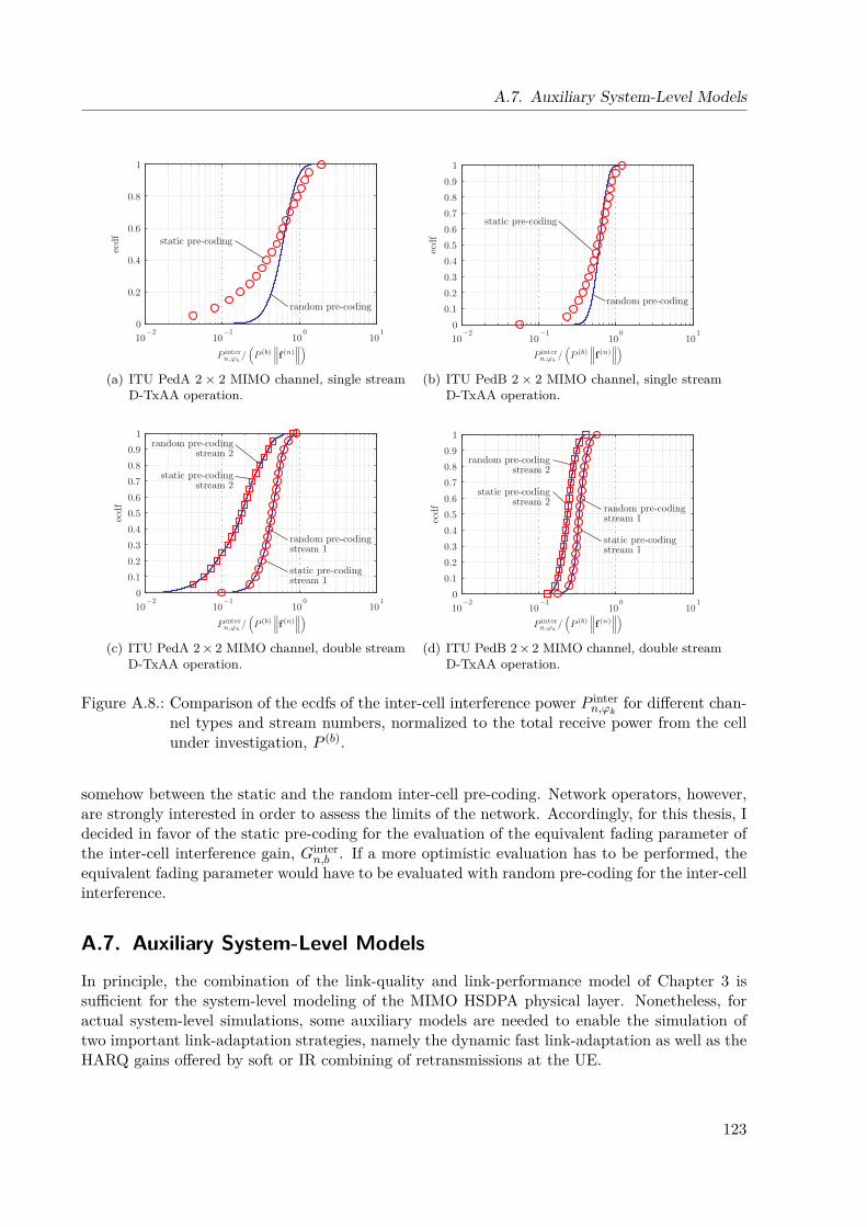
A.7. Auxiliary System-Level Models
10−2
10−1
100
101
0
0.2
0.4
0.6
0.8
1
ecdf
random pre-coding
static pre-coding
(a) ITU PedA 2 × 2 MIMO channel, single streamD-TxAA operation.
10−2
10−1
100
101
0
0.1
0.2
0.3
0.4
0.5
0.6
0.7
0.8
0.9
1
ecdf
random pre-coding
static pre-coding
(b) ITU PedB 2 × 2 MIMO channel, single streamD-TxAA operation.
10−2
10−1
100
101
0
0.1
0.2
0.3
0.4
0.5
0.6
0.7
0.8
0.9
1
ecdf
random pre-codingstream 1
random pre-codingstream 2
static pre-codingstream 1
static pre-codingstream 2
(c) ITU PedA 2× 2 MIMO channel, double streamD-TxAA operation.
10−2
10−1
100
101
0
0.1
0.2
0.3
0.4
0.5
0.6
0.7
0.8
0.9
1ec
df random pre-codingstream 1
random pre-codingstream 2
static pre-codingstream 1
static pre-codingstream 2
(d) ITU PedB 2× 2 MIMO channel, double streamD-TxAA operation.
Figure A.8.: Comparison of the ecdfs of the inter-cell interference power P intern,ϕk
for different chan-nel types and stream numbers, normalized to the total receive power from the cellunder investigation, P (b).
somehow between the static and the random inter-cell pre-coding. Network operators, however,are strongly interested in order to assess the limits of the network. Accordingly, for this thesis, Idecided in favor of the static pre-coding for the evaluation of the equivalent fading parameter ofthe inter-cell interference gain, Ginter
n,b . If a more optimistic evaluation has to be performed, theequivalent fading parameter would have to be evaluated with random pre-coding for the inter-cellinterference.
A.7. Auxiliary System-Level ModelsIn principle, the combination of the link-quality and link-performance model of Chapter 3 issufficient for the system-level modeling of the MIMO HSDPA physical layer. Nonetheless, foractual system-level simulations, some auxiliary models are needed to enable the simulation oftwo important link-adaptation strategies, namely the dynamic fast link-adaptation as well as theHARQ gains offered by soft or IR combining of retransmissions at the UE.
123
Appendix A. Additional Material
A.7.1. SINR-to-CQI MappingThe SINR-to-CQI mapping is needed to enable the fast TTI-based link-adaptation that hasbeen introduced with Release 5 HSDPA. As explained in Chapter 2, in order for the NodeB toadapt the downlink transmission to the current channel quality, the UE sends a CQI feedback.According to [7], this CQI feedback is defined as follows:
Based on an unrestricted observation interval, the UE shall report the highest tab-ulated CQI value for which a single HS-DSCH sub-frame formatted with the TBS,number of HS-PDSCH codes and modulation corresponding to the reported or lowerCQI value could be received with a transport block error probability not exceeding0.1 in a 3-slot reference period ending one slot before the start of the first slot inwhich the reported CQI value is transmitted.
Accordingly, the UE has to assess for every8 TTI which transport format associated to a CQIwould be the best in terms of largest TBS that does not exceed an average expected BLER of0.1. Given the identified possibility of modeling the BLER of the downlink by means of theMIESM effective SINR mapping/compression, it is straightforward to use this model also for theassessment of the SINR-to-CQI mapping.
Let me first define the mapping fCQI from the effective SINR, SINReffn , to the feedback CQI
c(F)n of stream n, as
fCQI(UE capability) : SINReffn 7→ c(F)
n , (A.22)which is a function of the UE capability class. Then, the proposed mapping is determined by the0.1 BLER points of the AWGN reference performance curves, obtained by the extensive link-levelsimulations for the derivation of the link-performance model. A similar approach has also beenproposed by the RAN working groups of 3GPP [39].
Figure A.9 shows the set of AWGN reference performance curves for UE capability Tables Dand I, which contain the same curves that were used in the MIESM mapping/compression trainingin Figures 3.13 to 3.15. Below the set of AWGN curves, the SINR-to-CQI mapping fCQI for eachUE capability table is shown, respectively. The mapping is obtained by finding the 0.1 BLERcrossing points in the SINR domain, marking the lowest channel-quality in SINR that supportsa downlink transmission with the TFC associated to the AWGN curve corresponding CQI c(F).The stair function denotes that a given CQI is reported as long as no higher TFC can achieve anpredicted BLER of at most 0.1.9 It has to be noted that the plots in Figure A.9 are shown as afunction of the HS-DSCH SINR instead of the HS-PDSCH SINR like in the MIESM training. Thereason for this is that a mapping in the HS-PDSCH SINR domain would lead to an ambiguous(not one-to-one) mapping. The HS-DSCH SINR for this purpose is evaluated as proposed in [39],by summing over all HS-PDSCH despreader outputs,
SINRHS-DSCHn =
∑ϕk∈Φ
SINRHS-PDSCHn , (A.23)
which in the effective SINR domain can be interpreted as adding 10 log10 |Φn| in the dB scale.If the set of AWGN target BLER crossing points and corresponding transmit CQI values, c(T)
n ,is denoted by
B(UE capability) =
(c(T)n ,SINR at target BLER)
, (A.24)
8In a practical network implementation, the CQI reporting period can be defined in multiples of a sub-frame [180].9Note that this suggests the application of a floor operation, like in [39] where CQI = bSNR[dB] + 3.5c as a
mapping is proposed.
124
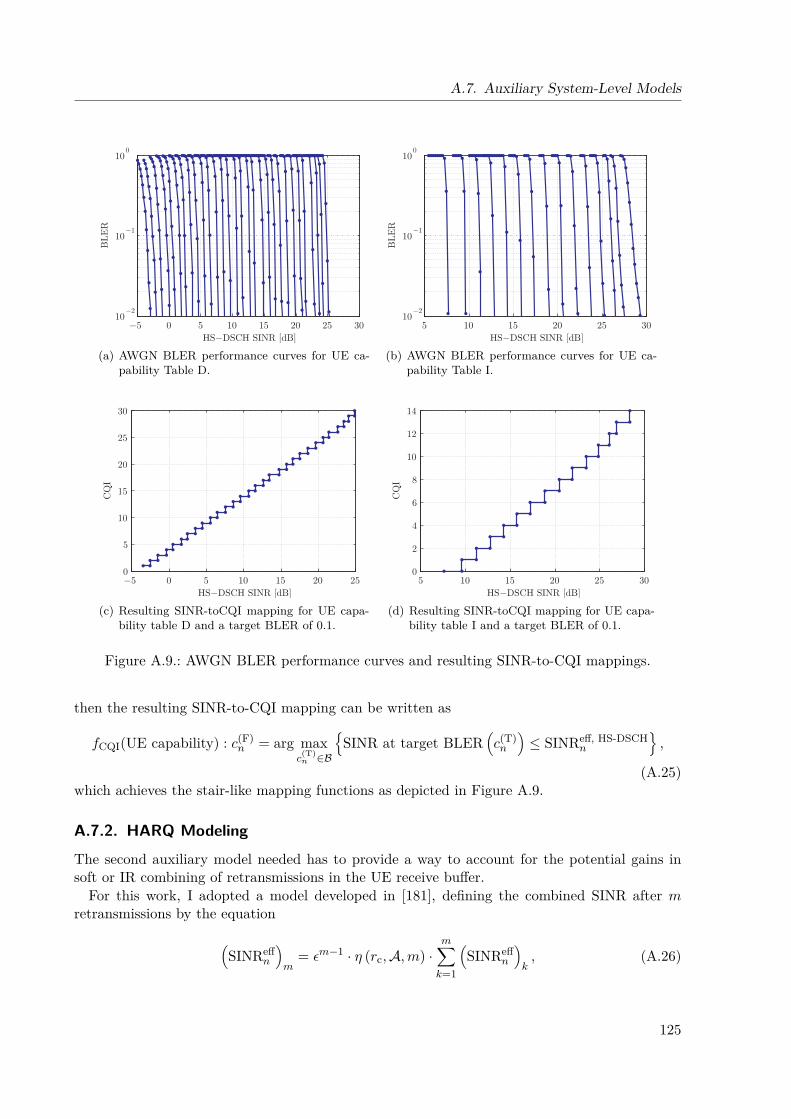
A.7. Auxiliary System-Level Models
−5 0 5 10 15 20 25 3010
−2
10−1
100
HS−DSCH SINR [dB]
BLE
R
(a) AWGN BLER performance curves for UE ca-pability Table D.
5 10 15 20 25 3010
−2
10−1
100
HS−DSCH SINR [dB]
BLE
R
(b) AWGN BLER performance curves for UE ca-pability Table I.
−5 0 5 10 15 20 250
5
10
15
20
25
30
HS−DSCH SINR [dB]
CQ
I
(c) Resulting SINR-toCQI mapping for UE capa-bility table D and a target BLER of 0.1.
5 10 15 20 25 300
2
4
6
8
10
12
14
HS−DSCH SINR [dB]
CQ
I
(d) Resulting SINR-toCQI mapping for UE capa-bility table I and a target BLER of 0.1.
Figure A.9.: AWGN BLER performance curves and resulting SINR-to-CQI mappings.
then the resulting SINR-to-CQI mapping can be written as
fCQI(UE capability) : c(F)n = arg max
c(T)n ∈B
SINR at target BLER
(c(T)n
)≤ SINReff, HS-DSCH
n
,
(A.25)which achieves the stair-like mapping functions as depicted in Figure A.9.
A.7.2. HARQ Modeling
The second auxiliary model needed has to provide a way to account for the potential gains insoft or IR combining of retransmissions in the UE receive buffer.
For this work, I adopted a model developed in [181], defining the combined SINR after mretransmissions by the equation
(SINReff
n
)m
= εm−1 · η (rc,A,m) ·m∑k=1
(SINReff
n
)k, (A.26)
125
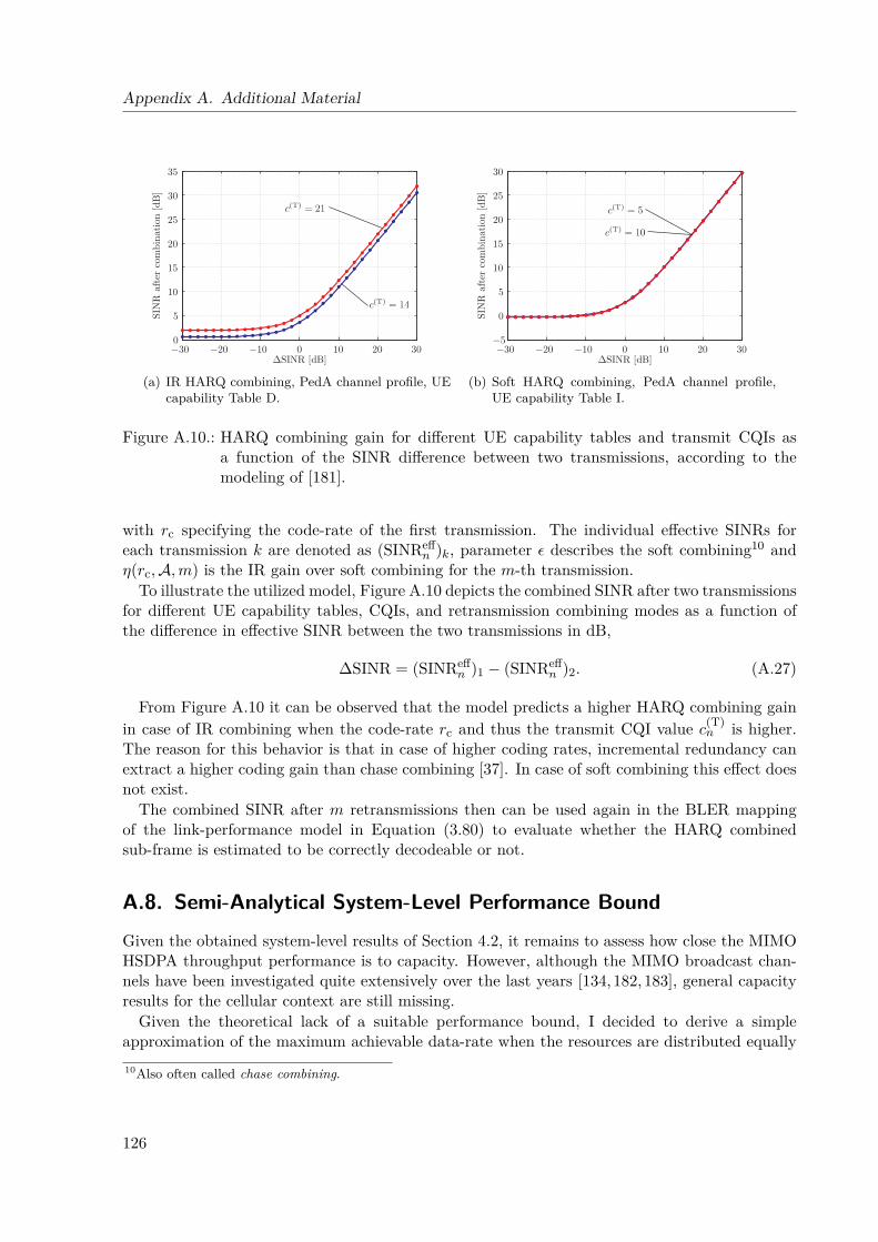
Appendix A. Additional Material
−30 −20 −10 0 10 20 300
5
10
15
20
25
30
35
SIN
R a
fter
com
bina
tion
[dB
]
(a) IR HARQ combining, PedA channel profile, UEcapability Table D.
−30 −20 −10 0 10 20 30−5
0
5
10
15
20
25
30
SIN
R a
fter
com
bina
tion
[dB
]
(b) Soft HARQ combining, PedA channel profile,UE capability Table I.
Figure A.10.: HARQ combining gain for different UE capability tables and transmit CQIs asa function of the SINR difference between two transmissions, according to themodeling of [181].
with rc specifying the code-rate of the first transmission. The individual effective SINRs foreach transmission k are denoted as (SINReff
n )k, parameter ε describes the soft combining10 andη(rc,A,m) is the IR gain over soft combining for the m-th transmission.
To illustrate the utilized model, Figure A.10 depicts the combined SINR after two transmissionsfor different UE capability tables, CQIs, and retransmission combining modes as a function ofthe difference in effective SINR between the two transmissions in dB,
∆SINR = (SINReffn )1 − (SINReff
n )2. (A.27)
From Figure A.10 it can be observed that the model predicts a higher HARQ combining gainin case of IR combining when the code-rate rc and thus the transmit CQI value c(T)
n is higher.The reason for this behavior is that in case of higher coding rates, incremental redundancy canextract a higher coding gain than chase combining [37]. In case of soft combining this effect doesnot exist.
The combined SINR after m retransmissions then can be used again in the BLER mappingof the link-performance model in Equation (3.80) to evaluate whether the HARQ combinedsub-frame is estimated to be correctly decodeable or not.
A.8. Semi-Analytical System-Level Performance Bound
Given the obtained system-level results of Section 4.2, it remains to assess how close the MIMOHSDPA throughput performance is to capacity. However, although the MIMO broadcast chan-nels have been investigated quite extensively over the last years [134, 182, 183], general capacityresults for the cellular context are still missing.
Given the theoretical lack of a suitable performance bound, I decided to derive a simpleapproximation of the maximum achievable data-rate when the resources are distributed equally10Also often called chase combining.
126
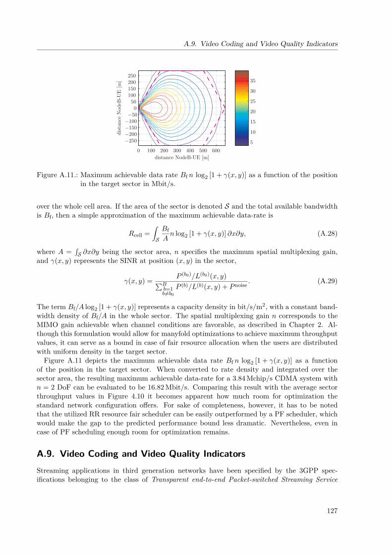
A.9. Video Coding and Video Quality Indicators
0 100 200 300 400 500 600
−250−200−150−100−50
050
100150200250
distance NodeB-UE [m]
dist
ance
Nod
eB-U
E [m
]
5
10
15
20
25
30
35
Figure A.11.: Maximum achievable data rate Bf n log2 [1 + γ(x, y)] as a function of the positionin the target sector in Mbit/s.
over the whole cell area. If the area of the sector is denoted S and the total available bandwidthis Bf, then a simple approximation of the maximum achievable data-rate is
Rcell =∫S
BfAn log2 [1 + γ(x, y)] ∂x∂y, (A.28)
where A =∫S ∂x∂y being the sector area, n specifies the maximum spatial multiplexing gain,
and γ(x, y) represents the SINR at position (x, y) in the sector,
γ(x, y) = P (b0)/L(b0)(x, y)∑Bb=1b6=b0
P (b)/L(b)(x, y) + P noise. (A.29)
The term Bf/A log2 [1 + γ(x, y)] represents a capacity density in bit/s/m2, with a constant band-width density of Bf/A in the whole sector. The spatial multiplexing gain n corresponds to theMIMO gain achievable when channel conditions are favorable, as described in Chapter 2. Al-though this formulation would allow for manyfold optimizations to achieve maximum throughputvalues, it can serve as a bound in case of fair resource allocation when the users are distributedwith uniform density in the target sector.
Figure A.11 depicts the maximum achievable data rate Bf n log2 [1 + γ(x, y)] as a functionof the position in the target sector. When converted to rate density and integrated over thesector area, the resulting maximum achievable data-rate for a 3.84 Mchip/s CDMA system withn = 2 DoF can be evaluated to be 16.82 Mbit/s. Comparing this result with the average sectorthroughput values in Figure 4.10 it becomes apparent how much room for optimization thestandard network configuration offers. For sake of completeness, however, it has to be notedthat the utilized RR resource fair scheduler can be easily outperformed by a PF scheduler, whichwould make the gap to the predicted performance bound less dramatic. Nevertheless, even incase of PF scheduling enough room for optimization remains.
A.9. Video Coding and Video Quality IndicatorsStreaming applications in third generation networks have been specified by the 3GPP spec-ifications belonging to the class of Transparent end-to-end Packet-switched Streaming Service
127
Appendix A. Additional Material
(PSS). Since the seventh release of [184], defining the mandatory and suggested codecs, theH.264/AVC [185] is mentioned as suggested video codec. The H.264/AVC, jointly standard-ized by the International Standard Organization (ISO) Moving Picture Expert Group (MPEG)and ITU Video Coding Expert Group (VCEG), is currently the state-of-the art video codec forcommercial applications. Thus, the coded utilized for the investigations in Section 4.4 was alsochosen to be H.264/AVC [19,20].
The H.264/AVC belongs to the family of the hybrid block based video codecs. These kinds ofvideo codecs exploit the correlation of small regions of the sequence pictures in space and in time.Each sample of the raw video sequence, a video frame, is subdivided into square blocks, calledMacroBlocks (MBs). Depending on the frame type, two encoding strategies are allowed. Themacroblocks belonging to Intra (I) predicted frames are encoded using the neighboring blocksof the same picture as a source of prediction. For Inter (P) predicted frames, the predictionis searched in the previously encoded pictures. In both cases, the prediction is then refined bymeans of frequency transformed residuals, representing the difference between the original blockand the best prediction.
The video encoder has been conceptually subdivided into two functional blocks. The VideoCoding Layer (VCL) deals with the proper encoding functionalities whereas the NAL providesnetwork friendliness to the produced data stream, managing the segmentation of the code intoNAL Units and reducing the dependency of the data stored in different packets. The maximumsize of a NAL unit is specified depending on the network Maximum Transfer Unit (MTU).Therefore, a NAL unit contains a variable number of MBs, representing a picture slice, dependingon the effectiveness of the considered prediction. For video streaming over third generationnetworks, the NAL units are further encapsulated into Real-time Transport Protocol (RTP),User Datagram Protocol (UDP) and, finally, IP.
Because of bad channel conditions and/or network congestion, some packet might not be cor-rectly received. At the decoder side error concealment techniques reduce the impact of missingpackets. Because of the temporal prediction, a missing packet does not only affect the recon-struction of the picture slice it contains but rather all the frames that use that slice as a sourceof prediction. This effect is referred to as temporal error propagation. The temporal error prop-agation ceases with the following I frame. Packets containing intra encoded information are selfcontained, i.e. the slice they contain can be reconstructed without the need of information storedin other packets.
The distance, in number of frames, between two consecutive I frames is defined as GOP. Thesize of the GOP has a strong impact on the quality of the receiver side: small GOPs reduce thetemporal propagation of the error. On the other hand, the spatial prediction used in the I framesis much less effective than the temporal one, particularly for high frequency patterns.
Since the error propagation is terminated by a correctly received I frame, preserving thepayload of the packets containing encoded I slices is of major importance with respect to theone containing P slices. However, within the P frames of a GOP, one can differentiate betweenP packets of different importance. Different works in the literature, deal with the unequal errorprotection of video packets, depending on the impact on the quality the slice they contain have.These methods often call for refined rate distortion analysis and limit the observation on thepunctual frame the slice belongs to.
Finally, let me recall that the PSNR has been chosen as video quality performance metric dueto its connection to the QoE. Further details on this relation can be found in [186] and referencestherein.
128
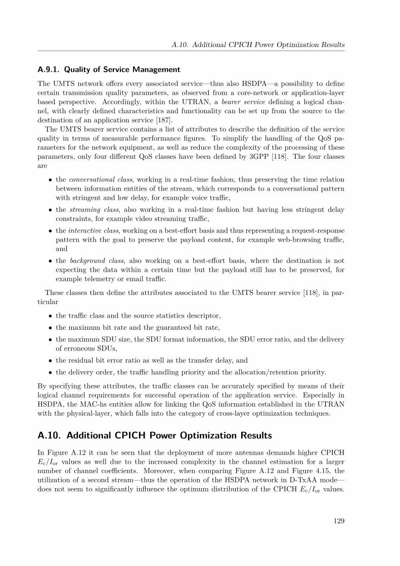
A.10. Additional CPICH Power Optimization Results
A.9.1. Quality of Service ManagementThe UMTS network offers every associated service—thus also HSDPA—a possibility to definecertain transmission quality parameters, as observed from a core-network or application-layerbased perspective. Accordingly, within the UTRAN, a bearer service defining a logical chan-nel, with clearly defined characteristics and functionality can be set up from the source to thedestination of an application service [187].
The UMTS bearer service contains a list of attributes to describe the definition of the servicequality in terms of measurable performance figures. To simplify the handling of the QoS pa-rameters for the network equipment, as well as reduce the complexity of the processing of theseparameters, only four different QoS classes have been defined by 3GPP [118]. The four classesare
• the conversational class, working in a real-time fashion, thus preserving the time relationbetween information entities of the stream, which corresponds to a conversational patternwith stringent and low delay, for example voice traffic,• the streaming class, also working in a real-time fashion but having less stringent delay
constraints, for example video streaming traffic,• the interactive class, working on a best-effort basis and thus representing a request-response
pattern with the goal to preserve the payload content, for example web-browsing traffic,and• the background class, also working on a best-effort basis, where the destination is not
expecting the data within a certain time but the payload still has to be preserved, forexample telemetry or email traffic.
These classes then define the attributes associated to the UMTS bearer service [118], in par-ticular
• the traffic class and the source statistics descriptor,• the maximum bit rate and the guaranteed bit rate,• the maximum SDU size, the SDU format information, the SDU error ratio, and the delivery
of erroneous SDUs,• the residual bit error ratio as well as the transfer delay, and• the delivery order, the traffic handling priority and the allocation/retention priority.
By specifying these attributes, the traffic classes can be accurately specified by means of theirlogical channel requirements for successful operation of the application service. Especially inHSDPA, the MAC-hs entities allow for linking the QoS information established in the UTRANwith the physical-layer, which falls into the category of cross-layer optimization techniques.
A.10. Additional CPICH Power Optimization ResultsIn Figure A.12 it can be seen that the deployment of more antennas demands higher CPICHEc/Ior values as well due to the increased complexity in the channel estimation for a largernumber of channel coefficients. Moreover, when comparing Figure A.12 and Figure 4.15, theutilization of a second stream—thus the operation of the HSDPA network in D-TxAA mode—does not seem to significantly influence the optimum distribution of the CPICH Ec/Ior values.
129
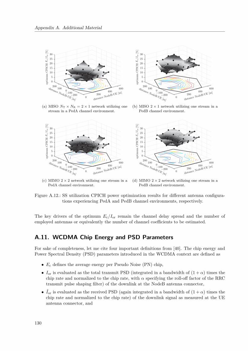
Appendix A. Additional Material
0200
400600
−200−1000
100200
0
5
10
15
20
25
30
distance NodeB-UE [m]
optim
um C
PIC
H[%
]
distance NodeB-UE [m]
(a) MISO NT × NR = 2 × 1 network utilizing onestream in a PedA channel environment.
0200
400600
−200−1000
100200
0
5
10
15
20
25
30
distance NodeB-UE [m]
optim
um C
PIC
H[%
]
distance NodeB-UE [m]
(b) MISO 2 × 1 network utilizing one stream in aPedB channel environment.
0200
400600
−200−1000
100200
0
5
10
15
20
25
30
distance NodeB-UE [m]
optim
um C
PIC
H[%
]
distance NodeB-UE [m]
(c) MIMO 2 × 2 network utilizing one stream in aPedA channel environment.
0200
400600
−200−1000
100200
0
5
10
15
20
25
30
distance NodeB-UE [m]
optim
um C
PIC
H[%
]
distance NodeB-UE [m]
(d) MIMO 2 × 2 network utilizing one stream in aPedB channel environment.
Figure A.12.: SS utilization CPICH power optimization results for different antenna configura-tions experiencing PedA and PedB channel environments, respectively.
The key drivers of the optimum Ec/Ior remain the channel delay spread and the number ofemployed antennas or equivalently the number of channel coefficients to be estimated.
A.11. WCDMA Chip Energy and PSD Parameters
For sake of completeness, let me cite four important definitions from [40]. The chip energy andPower Spectral Density (PSD) parameters introduced in the WCDMA context are defined as
• Ec defines the average energy per Pseudo Noise (PN) chip,
• Ior is evaluated as the total transmit PSD (integrated in a bandwidth of (1 + α) times thechip rate and normalized to the chip rate, with α specifying the roll-off factor of the RRCtransmit pulse shaping filter) of the downlink at the NodeB antenna connector,
• Ior is evaluated as the received PSD (again integrated in a bandwidth of (1 + α) times thechip rate and normalized to the chip rate) of the downlink signal as measured at the UEantenna connector, and
130
A.12. Calculating the Effective Code-Rate
• Ioc is evaluated as the PSD (integrated in a noise bandwidth equal to the chip rate andnormalized to the chip rate) of a band-limited white noise source (simulating interferencefrom other cells, which are not defined in a test procedure) as measured at the UE antennaconnector.
A.12. Calculating the Effective Code-Rate
Let me address here how the effective code-rate in the context of HSDPA is calculated. Asmentioned in Chapter 2, the number of bits transmitted utilizing one sub-frame is specified bythe UE capability table and the TFCI. In the context of the MIESM training of Chapter 3,the transmission format is chosen from the set of CQI values, thus being fully specified bythe according 3GPP CQI tables, in particular Table D and Table I. Furthermore, the timingconventions for HSDPA are that one HS-PDSCH sub-frame consists of 3 × 2560 chips, since itconsists of three slots with 2560 chips each. The number of symbols that can be transmittedusing one HS-PDSCH thus is given by 3 · 2560/16 since the spreading factor is fixed to SF = 16for HSDPA. Accordingly, the total available number of bits per sub-frame can be evaluated byconsidering the number of bits per symbol, log2 |A|, and the number of HS-PDSCHs, |Φ|, thusleading to 3 ·2560/16 · log2 |A| · |Φ|. Denoting the TBS of the transmit CQI c(T) to be TBS(c(T)),the effective code-rate is given by
rc =TBS
(c(T)
)3·2560
16 log2 |A| · |Φ|.
A.13. Validation of the System-Level Simulator with Odyssey Data
The work presented in Chapter 4 is based on a generic regular network structure that is designedto represent realistic cellular environments. However, in reality, network operators have to planand deploy their networks according to many restrictions and constraints so that the resultingnetwork layouts diverge often significantly from regular and symmetric structures.
For planing purposes network operators utilize special tools [10, 111] to predict the influencesof electrical and mechanical tilts and azimuth of the deployed antennas. These tools usually relyon path-loss maps of the network region generated from ray-tracing models that are calibratedby field measurements. These maps also sometimes also serve to assess the expected trafficthroughput per day/week which is needed in order to do suitable backhaul capacity planing.
In order to evaluate the validity of the developed system-level simulator, mobilkom austria AGprovided path-loss and network setup data for a specific region in Vienna where HSDPA trialruns were conducted. The provided data included
• the positions of the NodeBs included in the trial run,
• the sector antenna azimuths,
• path-loss data files with 10 m resolution for all NodeBs,
• maximum transmit power values for all NodeBs, and
• the resulting ecdf of the CPICH Ec/Ioc for every sector.
131
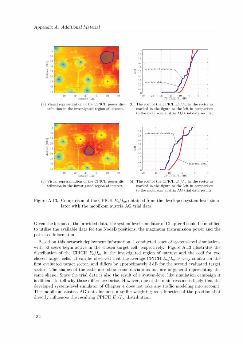
Appendix A. Additional Material
distance [10m]
dist
ance
[10
m]
10 20 30 40 50 60
5
10
15
20
25
30
35
40
45
(a) Visual representation of the CPICH power dis-tribution in the investigated region of interest.
−30 −25 −20 −15 −10 −5 0 50
0.1
0.2
0.3
0.4
0.5
0.6
0.7
0.8
0.9
1
ecdf
mka trial data
system-level simulation
(b) The ecdf of the CPICH Ec/Ioc in the sector asmarked in the figure to the left in comparisonto the mobilkom austria AG trial data results.
distance [10m]
dist
ance
[10
m]
10 20 30 40 50 60
5
10
15
20
25
30
35
40
45
(c) Visual representation of the CPICH power dis-tribution in the investigated region of interest.
−20 −15 −10 −5 0 50
0.1
0.2
0.3
0.4
0.5
0.6
0.7
0.8
0.9
1
ecdf
system-level simulation
mka trial data
(d) The ecdf of the CPICH Ec/Ioc in the sector asmarked in the figure to the left in comparisonto the mobilkom austria AG trial data results.
Figure A.13.: Comparison of the CPICH Ec/Ioc obtained from the developed system-level simu-lator with the mobilkom austria AG trial data.
Given the format of the provided data, the system-level simulator of Chapter 4 could be modifiedto utilize the available data for the NodeB positions, the maximum transmission power and thepath-loss information.
Based on this network deployment information, I conducted a set of system-level simulationswith 50 users begin active in the chosen target cell, respectively. Figure A.13 illustrates thedistribution of the CPICH Ec/Ioc in the investigated region of interest and the ecdf for twochosen target cells. It can be observed that the average CPICH Ec/Ioc is very similar for thefirst evaluated target sector, and differs by approximately 3 dB for the second evaluated targetsector. The shapes of the ecdfs also show some deviations but are in general representing thesame shape. Since the trial data is also the result of a system-level like simulation campaign itis difficult to tell why these differences arise. However, one of the main reasons is likely that thedeveloped system-level simulator of Chapter 4 does not take any traffic modeling into account.The mobilkom austria AG data includes a traffic weighting as a function of the position thatdirectly influences the resulting CPICH Ec/Ioc distribution.
132
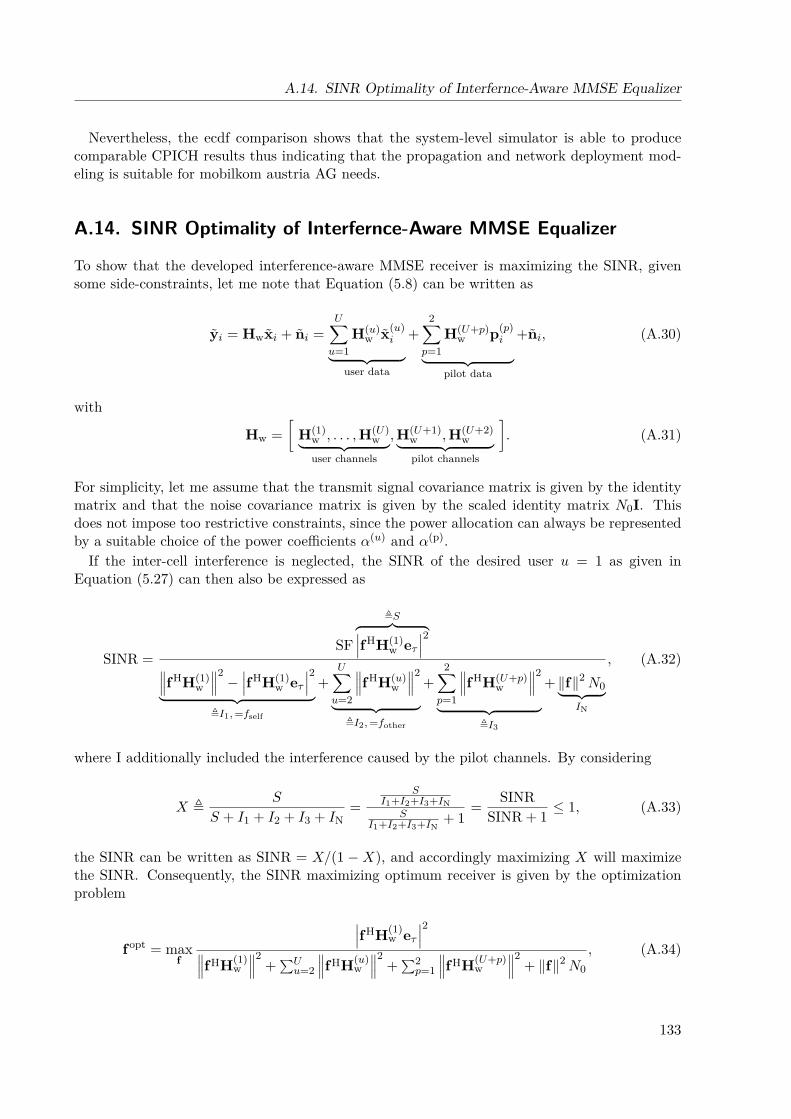
A.14. SINR Optimality of Interfernce-Aware MMSE Equalizer
Nevertheless, the ecdf comparison shows that the system-level simulator is able to producecomparable CPICH results thus indicating that the propagation and network deployment mod-eling is suitable for mobilkom austria AG needs.
A.14. SINR Optimality of Interfernce-Aware MMSE Equalizer
To show that the developed interference-aware MMSE receiver is maximizing the SINR, givensome side-constraints, let me note that Equation (5.8) can be written as
yi = Hwxi + ni =U∑u=1
H(u)w x(u)
i︸ ︷︷ ︸user data
+2∑p=1
H(U+p)w p(p)
i︸ ︷︷ ︸pilot data
+ni, (A.30)
with
Hw =[
H(1)w , . . . ,H(U)
w︸ ︷︷ ︸user channels
,H(U+1)w ,H(U+2)
w︸ ︷︷ ︸pilot channels
]. (A.31)
For simplicity, let me assume that the transmit signal covariance matrix is given by the identitymatrix and that the noise covariance matrix is given by the scaled identity matrix N0I. Thisdoes not impose too restrictive constraints, since the power allocation can always be representedby a suitable choice of the power coefficients α(u) and α(p).
If the inter-cell interference is neglected, the SINR of the desired user u = 1 as given inEquation (5.27) can then also be expressed as
SINR =SF
,S︷ ︸︸ ︷∣∣∣fHH(1)w eτ
∣∣∣2∥∥∥fHH(1)w
∥∥∥2−∣∣∣fHH(1)
w eτ∣∣∣2︸ ︷︷ ︸
,I1,=fself
+U∑u=2
∥∥∥fHH(u)w
∥∥∥2
︸ ︷︷ ︸,I2,=fother
+2∑p=1
∥∥∥fHH(U+p)w
∥∥∥2
︸ ︷︷ ︸,I3
+ ‖f‖2N0︸ ︷︷ ︸IN
, (A.32)
where I additionally included the interference caused by the pilot channels. By considering
X ,S
S + I1 + I2 + I3 + IN=
SI1+I2+I3+IN
SI1+I2+I3+IN
+ 1= SINR
SINR + 1 ≤ 1, (A.33)
the SINR can be written as SINR = X/(1 −X), and accordingly maximizing X will maximizethe SINR. Consequently, the SINR maximizing optimum receiver is given by the optimizationproblem
fopt = maxf
∣∣∣fHH(1)w eτ
∣∣∣2∥∥∥fHH(1)w∥∥∥2
+∑Uu=2
∥∥∥fHH(u)w∥∥∥2
+∑2p=1
∥∥∥fHH(U+p)w
∥∥∥2+ ‖f‖2N0
, (A.34)
133
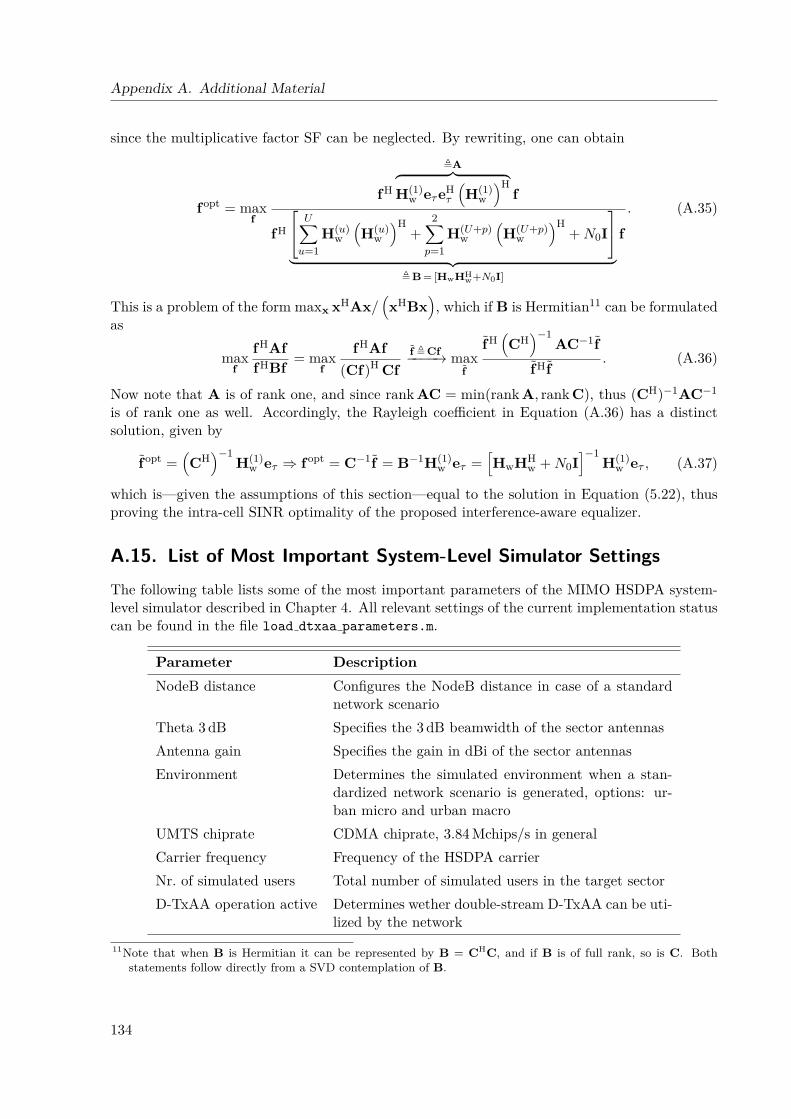
Appendix A. Additional Material
since the multiplicative factor SF can be neglected. By rewriting, one can obtain
fopt = maxf
fH
,A︷ ︸︸ ︷H(1)
w eτeHτ
(H(1)
w
)Hf
fH
U∑u=1
H(u)w
(H(u)
w
)H+
2∑p=1
H(U+p)w
(H(U+p)
w
)H+N0I
︸ ︷︷ ︸
,B = [HwHHw+N0I]
f
. (A.35)
This is a problem of the form maxx xHAx/(xHBx
), which if B is Hermitian11 can be formulated
as
maxf
fHAffHBf = max
f
fHAf(Cf)H Cf
f ,Cf−−−−→ maxf
fH(CH
)−1AC−1f
fHf. (A.36)
Now note that A is of rank one, and since rank AC = min(rank A, rank C), thus (CH)−1AC−1
is of rank one as well. Accordingly, the Rayleigh coefficient in Equation (A.36) has a distinctsolution, given by
fopt =(CH
)−1H(1)
w eτ ⇒ fopt = C−1f = B−1H(1)w eτ =
[HwHH
w +N0I]−1
H(1)w eτ , (A.37)
which is—given the assumptions of this section—equal to the solution in Equation (5.22), thusproving the intra-cell SINR optimality of the proposed interference-aware equalizer.
A.15. List of Most Important System-Level Simulator SettingsThe following table lists some of the most important parameters of the MIMO HSDPA system-level simulator described in Chapter 4. All relevant settings of the current implementation statuscan be found in the file load dtxaa parameters.m.
Parameter DescriptionNodeB distance Configures the NodeB distance in case of a standard
network scenarioTheta 3 dB Specifies the 3 dB beamwidth of the sector antennasAntenna gain Specifies the gain in dBi of the sector antennasEnvironment Determines the simulated environment when a stan-
dardized network scenario is generated, options: ur-ban micro and urban macro
UMTS chiprate CDMA chiprate, 3.84 Mchips/s in generalCarrier frequency Frequency of the HSDPA carrierNr. of simulated users Total number of simulated users in the target sectorD-TxAA operation active Determines wether double-stream D-TxAA can be uti-
lized by the network11Note that when B is Hermitian it can be represented by B = CHC, and if B is of full rank, so is C. Both
statements follow directly from a SVD contemplation of B.
134

A.15. List of Most Important System-Level Simulator Settings
Parameter DescriptionNr. of available HS-PDSCHs Specifies the number of spreading sequences available
for HSDPA operationMax. NodeB output power Determines the maximum NodeB output powerCPICH power Specifies the transmission power of the CPICH, in the
MIMO case the power spent for both CPICHOther channels power Determines the transmission power of all other signal-
ing and feedback channelsNr. of samples Specifies the number of simulated samples in slots and
thus the simulation lengthFeedback delay Determines the delay of the the UE feedback to arrive
at the NodeB entity in the simulatorMax. nr. of retransmissions Limits the maximum number of retransmissions avail-
able for the NodeB before marking a packet as non-deliverable
Scheduler type Sets the utilized scheduler, depending on the schedulerclass some further parameters then define its behavior
Nr. of transmit antennas —Nr. of receive antennas —UE capability class Specifies the UE capabilities in terms of maximum
throughput, retransmission combining and MIMO ca-pabilities. See also Chapter 2 for further details.
UE speed Determines the speed of the UEs for the movementthrough the sector
Receiver type Specifies the receiver type of the UE, options: MMSEand Rake
Equalizer span Specifies the length of the receive filter for all simu-lated UEs
Equalizer delay Specifies the delay of the receive filter for all simulatedUEs
135

Appendix B.
Further System-Level Modeling, Simulations,Optimizations, and Validation
You have to lay the groundworkahead of time. If you haven’t donethat, do it now.
(Lee Miller)
High speed data transmissions in wireless networks have effectively been enabled alreadywith the introduction of Release 5 HSDPA. Mobile wireless network operators have SISO
HSDPA networks deployed in many countries with different maximum up- and downlink speeds,see Chapter 2 for more information hereon. Accordingly, although SISO HSDPA has been activelybeen researched for many years now, some open questions still remain to be of interest, especiallyin the network context.
This thesis has been funded by one of the major network operators in Austria, the mobilkomaustria AG,1 which currently has the largest HSDPA deployment in Austria. Parts of the workpresented in this chapter also were of particular interest for their network deployment in 2006and 2007, when I started working as a doctoral candidate.
The consolidated findings of the work recapitulated in this chapter furthermore was veryhelpful in building the basic groundwork for the development of the more advanced system-levelmodels in Chapter 3, as well as the practical implementation of the system-level simulator inChapter 4 and the optimizations carried out with it. The presented work was partly publishedat international conferences [15, 26], but it has to be noted that not always every single aspecthas been deeply investigated due to the fact that MIMO techniques became the more importantfocus.
Finally, let me point out that the following sections contribute to a deeper understanding ofthe HSDPA performance in today’s networks, even for the MIMO enhancements. Accordingly, Iintended to include these to round-off the concept of this thesis.
B.1. Mixed Traffic Optimization for SISO HSDPA
As mentioned in Chapter 2, HSDPA is designed so that it can be operated within an existing5 MHz band that is already utilized by Release 4 DCHs, thus allowing for sharing the poweramplifier at the Node-B. Accordingly, one part of the available Node-B power and spreadingcodes is used for the DCHs and another part can be used for the HSDPA operation. Thisspecific mode of operation is of particular interest for the network operators in the phase of the
1AG is the German term for a public cooperation.
137
Appendix B. Further System-Level Modeling, Simulations, Optimizations, and Validation
HSDPA deployment, and even if HSDPA is widely installed, a mixed carrier operation is morecost-efficient for cells that are not fully loaded.
Despite the significance of the study of the network performance behavior in such a scenario,not much work has been performed in order to assess the average user throughput, the totalcell throughput, or to derive specific recommendations for the network planning process. Theavailable work discusses only a very limited part of the whole topic, for example [67], where onlythe ITU VehA channel profile has been considered. This is a fairly unusual since most of theHSDPA traffic occurring in a network will be requested by slowly moving UEs.
A big difference in the work presented in this section compared to Chapters 3 and 4 is that thesimulation approach is snapshot-based. This means that no correlation in time is considered, butthe rather a snapshot of the current network state is evaluated. By averaging over multiple ofthose snapshots, each with individual and independent channel realizations, the average networkperformance can be evaluated. However, such a modeling approach has the drawback that noenhanced scheduling mechanisms—which implicitly build upon the correlation of the channel intime—can be assessed. Nevertheless, the average results presented remain valid for RR schedulersthat do not take the reported CQI feedback into account.2
B.1.1. System Model
Channel Modeling
The radio propagation model throughout Appendix B.1 considers basically three different parts:macro-scale path-loss λm, shadow fading λs, and small-scale fading with multiple paths and nocorrelation in time. This corresponds to the restriction of the simulator to conduct only snapshotsimulations. Accordingly, the channel between the base station and the user equipment can bewritten as
hi = λm · λs ·Lh∑l=1
√pl · rl · δi−il , (B.1)
where the random variables rl represent Lh independent Rayleigh fading processes at fixed timeslots, δ denotes the Dirac function and pl, il are the relative power and delay of the multipathcomponents, according to the ITU channel profiles [159]. In contrast to Chapter 3, Lh denotesthe number of taps of the channel.
The macro-scale path-loss λm depends only on the distance d between the base station andthe user equipment, which I model according to the COST 231 Model [112]. The shadow fadingλs is modelled by a lognormal random variable with zero mean and variance σ2
λs= 8 dB, with no
correlation in time.
HSDPA Modeling
The necessary system-level modeling here is again split into a link-quality model and a link-performance model, as described in Chapter 3. For deriving the link-quality model, I assumed a
2The system-level simulator developed with the modeling and assumptions presented in this section formed thefirst implementation of a system-level simulator for HSDPA networks. However after having the system-levelmodel for MIMO HSDPA as presented in Chapter 3 developed, a new and more flexible simulator architecturewas implemented that succeeded this first version. Nevertheless, besides the work presented here, the SISOHSDPA system-level simulator proofed to be valuable for other investigations as well [188,189].
138
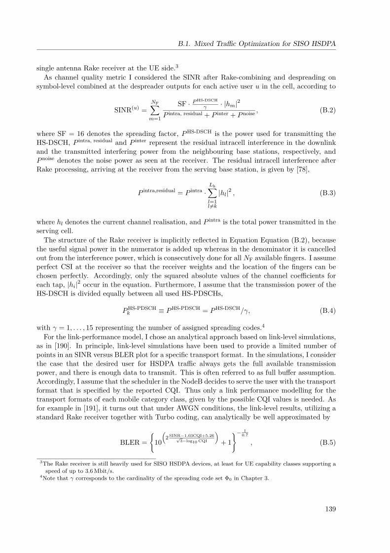
B.1. Mixed Traffic Optimization for SISO HSDPA
single antenna Rake receiver at the UE side.3As channel quality metric I considered the SINR after Rake-combining and despreading on
symbol-level combined at the despreader outputs for each active user u in the cell, according to
SINR(u) =NF∑m=1
SF · PHS-DSCH
γ · |hm|2
P intra, residual + P inter + P noise , (B.2)
where SF = 16 denotes the spreading factor, PHS-DSCH is the power used for transmitting theHS-DSCH, P intra, residual and P inter represent the residual intracell interference in the downlinkand the transmitted interfering power from the neighbouring base stations, respectively, andP noise denotes the noise power as seen at the receiver. The residual intracell interference afterRake processing, arriving at the receiver from the serving base station, is given by [78],
P intra,residual = P intra ·Lh∑l=1l 6=k
|hl|2 , (B.3)
where hl denotes the current channel realisation, and P intra is the total power transmitted in theserving cell.
The structure of the Rake receiver is implicitly reflected in Equation Equation (B.2), becausethe useful signal power in the numerator is added up whereas in the denominator it is cancelledout from the interference power, which is consecutively done for all NF available fingers. I assumeperfect CSI at the receiver so that the receiver weights and the location of the fingers can bechosen perfectly. Accordingly, only the squared absolute values of the channel coefficients foreach tap, |hi|2 occur in the equation. Furthermore, I assume that the transmission power of theHS-DSCH is divided equally between all used HS-PDSCHs,
PHS-PDSCHk ≡ PHS-PDSCH = PHS-DSCH/γ, (B.4)
with γ = 1, . . . , 15 representing the number of assigned spreading codes.4For the link-performance model, I chose an analytical approach based on link-level simulations,
as in [190]. In principle, link-level simulations have been used to provide a limited number ofpoints in an SINR versus BLER plot for a specific transport format. In the simulations, I considerthe case that the desired user for HSDPA traffic always gets the full available transmissionpower, and there is enough data to transmit. This is often referred to as full buffer assumption.Accordingly, I assume that the scheduler in the NodeB decides to serve the user with the transportformat that is specified by the reported CQI. Thus only a link performance modelling for thetransport formats of each mobile category class, given by the possible CQI values is needed. Asfor example in [191], it turns out that under AWGN conditions, the link-level results, utilizing astandard Rake receiver together with Turbo coding, can analytically be well approximated by
BLER =
10(
2 SINR−1.03CQI+5.26√3−log10 CQI
)+ 1
− 10.7
, (B.5)
3The Rake receiver is still heavily used for SISO HSDPA devices, at least for UE capability classes supporting aspeed of up to 3.6 Mbit/s.
4Note that γ corresponds to the cardinality of the spreading code set Φ0 in Chapter 3.
139
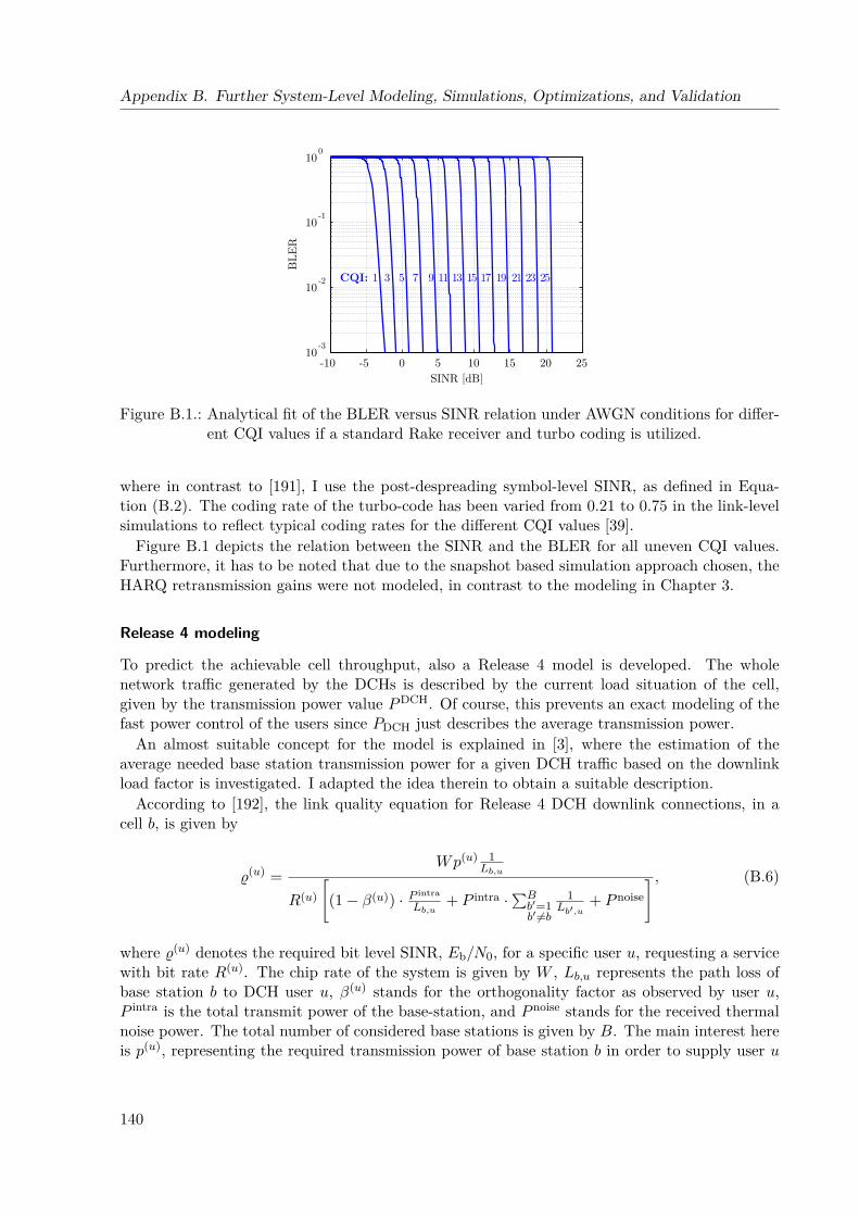
Appendix B. Further System-Level Modeling, Simulations, Optimizations, and Validation
-10 -5 0 5 10 15 20 2510
-3
10-2
10-1
100
SINR [dB]
BLE
RCQI: 1 3 5 7 9 11 13 15 17 19 21 23 25
Figure B.1.: Analytical fit of the BLER versus SINR relation under AWGN conditions for differ-ent CQI values if a standard Rake receiver and turbo coding is utilized.
where in contrast to [191], I use the post-despreading symbol-level SINR, as defined in Equa-tion (B.2). The coding rate of the turbo-code has been varied from 0.21 to 0.75 in the link-levelsimulations to reflect typical coding rates for the different CQI values [39].
Figure B.1 depicts the relation between the SINR and the BLER for all uneven CQI values.Furthermore, it has to be noted that due to the snapshot based simulation approach chosen, theHARQ retransmission gains were not modeled, in contrast to the modeling in Chapter 3.
Release 4 modeling
To predict the achievable cell throughput, also a Release 4 model is developed. The wholenetwork traffic generated by the DCHs is described by the current load situation of the cell,given by the transmission power value PDCH. Of course, this prevents an exact modeling of thefast power control of the users since PDCH just describes the average transmission power.
An almost suitable concept for the model is explained in [3], where the estimation of theaverage needed base station transmission power for a given DCH traffic based on the downlinkload factor is investigated. I adapted the idea therein to obtain a suitable description.
According to [192], the link quality equation for Release 4 DCH downlink connections, in acell b, is given by
%(u) =Wp(u) 1
Lb,u
R(u)
[(1− β(u)) · P intra
Lb,u+ P intra ·
∑Bb′=1b′ 6=b
1Lb′,u
+ P noise
] , (B.6)
where %(u) denotes the required bit level SINR, Eb/N0, for a specific user u, requesting a servicewith bit rate R(u). The chip rate of the system is given by W , Lb,u represents the path loss ofbase station b to DCH user u, β(u) stands for the orthogonality factor as observed by user u,P intra is the total transmit power of the base-station, and P noise stands for the received thermalnoise power. The total number of considered base stations is given by B. The main interest hereis p(u), representing the required transmission power of base station b in order to supply user u
140
B.1. Mixed Traffic Optimization for SISO HSDPA
with the defined service. The sum of it equals the DCH cell load,U∑u=1
p(u) = PDCH, (B.7)
with U denoting the total number of active DCH users in the cell.For modeling purpose, let me assume the same service for all DCH users in the cell, given by
the required bit level SINR and the requested rate,
%(u) ≡ %, R(u) ≡ R. (B.8)
In analogy to [3], I furthermore introduce the own cell to other cell interference ratio, given by
O =B∑b′=1b′ 6=b
Lb,uLb′,u
. (B.9)
Since the DCH users should not be modeled explicitly, I substituted O and Lb,u by their averagesover the cell area
O → O, Lb,u → Lb. (B.10)The orthogonality factor β can be calculated in a simple way as described in [78],
β(u) = 1−
Lh∑l=1
∣∣∣h(u)l
∣∣∣21−
∣∣∣h(u)l
∣∣∣2−1
, (B.11)
with h(u)l = √plr
(u)l describing the complex valued coefficient of the channel tap l, for each user
u, respectively.5 The user dependency in this case is only introduced because of the small-scalefading channel statistics. In analogy to the simplifications already introduced above, I substitutethe orthogonality factor β(u) by its average β, which is achieved by using the average channeltap values E
|hl|2
= pl, determined by the ITU channel profiles.
With this simplifications, and after some algebra, the number of DCH users that can be servedgiven a specific data rate can be derived to be
U = PDCH
P intra · %RW ·[(1− β) +O
]+ P noise · %RW · Lb
. (B.12)
Power split
The total available transmit power in each cell is shared between HSDPA and DCH users. Letme express the total intra-cell transmission power as
P intra = PDCH + PHS-DSCH + P other, (B.13)
where P other incorporates the power from other needed common channels, for example theCPICH. Accordingly, both, Equation (B.2) and Equation (B.12) depend on the transmissionpower of the DCH and the HSDPA traffic.
As described in Chapter 2, there are two different possibilities of allocating the power ofHSDPA in the base station downlink power budget [44], and both possibilities will be treated inthe following.
5Note that the channel power normalization requires the sum of the taps to equal one,∑Lh
l=1 |h(u)l |
2 = 1.
141
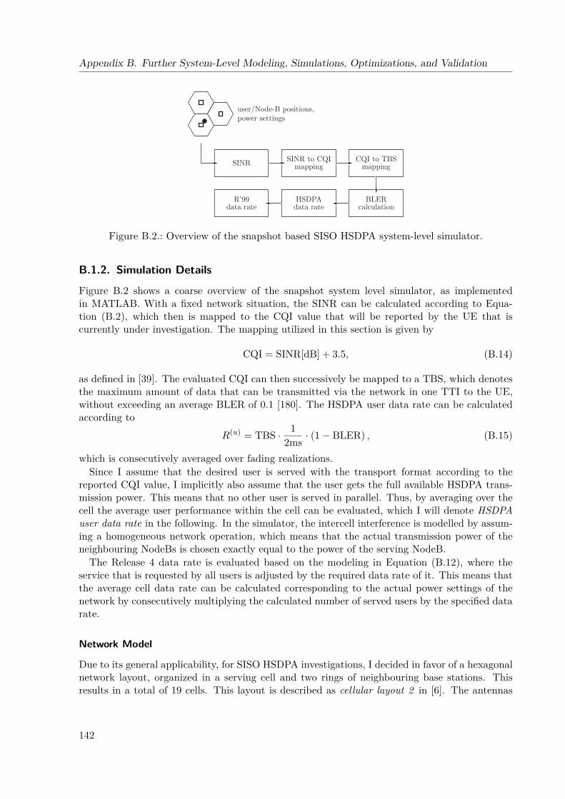
Appendix B. Further System-Level Modeling, Simulations, Optimizations, and Validation
user/Node-B positions,power settings
SINR SINR to CQImapping
CQI to TBSmapping
BLERcalculation
HSDPAdata rate
R’99data rate
Figure B.2.: Overview of the snapshot based SISO HSDPA system-level simulator.
B.1.2. Simulation Details
Figure B.2 shows a coarse overview of the snapshot system level simulator, as implementedin MATLAB. With a fixed network situation, the SINR can be calculated according to Equa-tion (B.2), which then is mapped to the CQI value that will be reported by the UE that iscurrently under investigation. The mapping utilized in this section is given by
CQI = SINR[dB] + 3.5, (B.14)
as defined in [39]. The evaluated CQI can then successively be mapped to a TBS, which denotesthe maximum amount of data that can be transmitted via the network in one TTI to the UE,without exceeding an average BLER of 0.1 [180]. The HSDPA user data rate can be calculatedaccording to
R(u) = TBS · 12ms · (1− BLER) , (B.15)
which is consecutively averaged over fading realizations.Since I assume that the desired user is served with the transport format according to the
reported CQI value, I implicitly also assume that the user gets the full available HSDPA trans-mission power. This means that no other user is served in parallel. Thus, by averaging over thecell the average user performance within the cell can be evaluated, which I will denote HSDPAuser data rate in the following. In the simulator, the intercell interference is modelled by assum-ing a homogeneous network operation, which means that the actual transmission power of theneighbouring NodeBs is chosen exactly equal to the power of the serving NodeB.
The Release 4 data rate is evaluated based on the modeling in Equation (B.12), where theservice that is requested by all users is adjusted by the required data rate of it. This means thatthe average cell data rate can be calculated corresponding to the actual power settings of thenetwork by consecutively multiplying the calculated number of served users by the specified datarate.
Network Model
Due to its general applicability, for SISO HSDPA investigations, I decided in favor of a hexagonalnetwork layout, organized in a serving cell and two rings of neighbouring base stations. Thisresults in a total of 19 cells. This layout is described as cellular layout 2 in [6]. The antennas
142
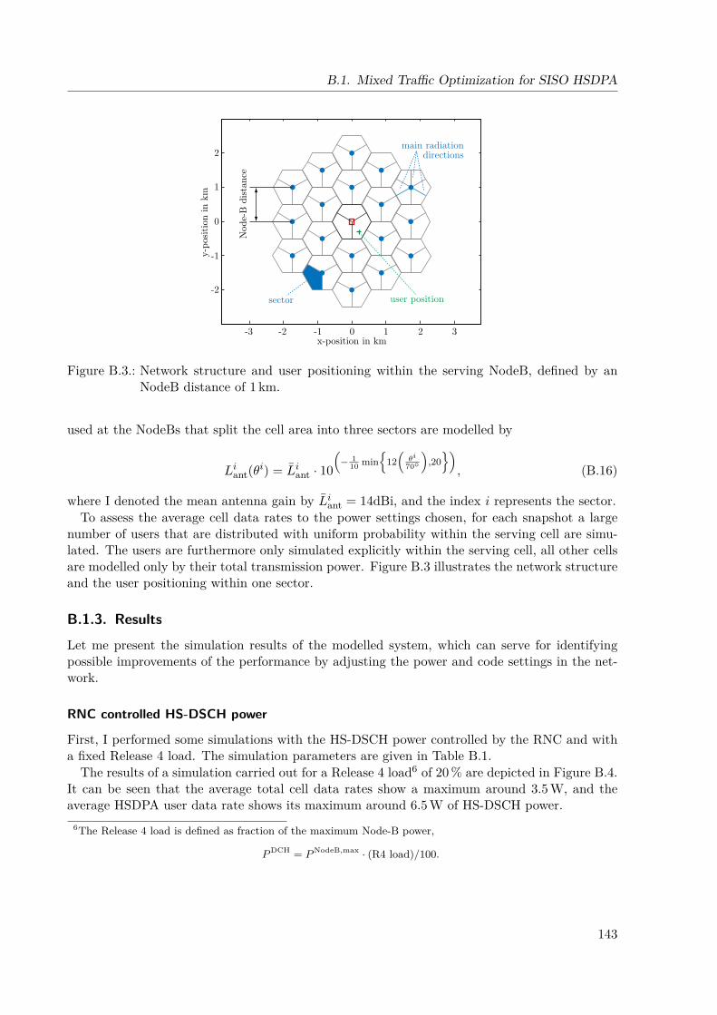
B.1. Mixed Traffic Optimization for SISO HSDPA
x-position in km
y-po
sition
in
km
-3 -2 -1 0 1 2 3
-2
-1
0
1
2main radiation
directions
Nod
e-B
dis
tanc
e
user positionsector
Figure B.3.: Network structure and user positioning within the serving NodeB, defined by anNodeB distance of 1 km.
used at the NodeBs that split the cell area into three sectors are modelled by
Liant(θi) = Liant · 10(− 1
10 min
12(θi
70
),20), (B.16)
where I denoted the mean antenna gain by Liant = 14dBi, and the index i represents the sector.To assess the average cell data rates to the power settings chosen, for each snapshot a large
number of users that are distributed with uniform probability within the serving cell are simu-lated. The users are furthermore only simulated explicitly within the serving cell, all other cellsare modelled only by their total transmission power. Figure B.3 illustrates the network structureand the user positioning within one sector.
B.1.3. Results
Let me present the simulation results of the modelled system, which can serve for identifyingpossible improvements of the performance by adjusting the power and code settings in the net-work.
RNC controlled HS-DSCH power
First, I performed some simulations with the HS-DSCH power controlled by the RNC and witha fixed Release 4 load. The simulation parameters are given in Table B.1.
The results of a simulation carried out for a Release 4 load6 of 20 % are depicted in Figure B.4.It can be seen that the average total cell data rates show a maximum around 3.5 W, and theaverage HSDPA user data rate shows its maximum around 6.5 W of HS-DSCH power.
6The Release 4 load is defined as fraction of the maximum Node-B power,
PDCH = PNodeB,max · (R4 load)/100.
143

Appendix B. Further System-Level Modeling, Simulations, Optimizations, and Validation
Table B.1.: Simulation parameters for the simulations with RNC controlled HS-DSCH power.Parameter ValueNodeB distance 0.75 kmmaximum NodeB power 43 dBmP other 33 dBmshadow fading variance 8 dBchannel type ITU PedAavailable HS-PDSCH codes 5HS-DSCH power variableUE capability class 6receiver noise figure 7 dBRake fingers 4Release 4 load fixed, 20 %DCH required service SINR % = 5.2 dBDCH service data rate R = 384 kbit/s
0 2 4 6 8 10 12 140
1
2
3
4
5
6
7
8
9x 10
5
PHS-DSCH
[W]
aver
age
data
rat
e
total cell data rate
HSDPA user data rate
Release ´99 cell data rate
maximum totalcell data rate
maximum HSDPAuser data rate
Figure B.4.: Average data rates evaluated according to the simulation settings in Table B.1 withRNC power control of the HS-DSCH.
Therefore, in case that the HS-DSCH power is RNC controlled, the optimum power settingdepending on the optimization criteria, which can be either the average HSDPA data rate or theaverage cell data rate, can be found. Furthermore, it can be seen that in case of an ITU PedAchannel profile, HSDPA offers a broad power operating range in which the throughput is nearlyoptimum.
By running a set of these simulations, I was able to analyse the relation between the HS-DSCH power level, at which the maximum of the average total cell data rate is achieved, andthe Release 4 load of the cell. The results are illustrated in Figure B.5, for different NodeBdistances. It can be seen that the optimum HS-DSCH power scales with the Release 4 load, butthen starts to drop down, which is caused by the limited maximum NodeB transmission power.
144
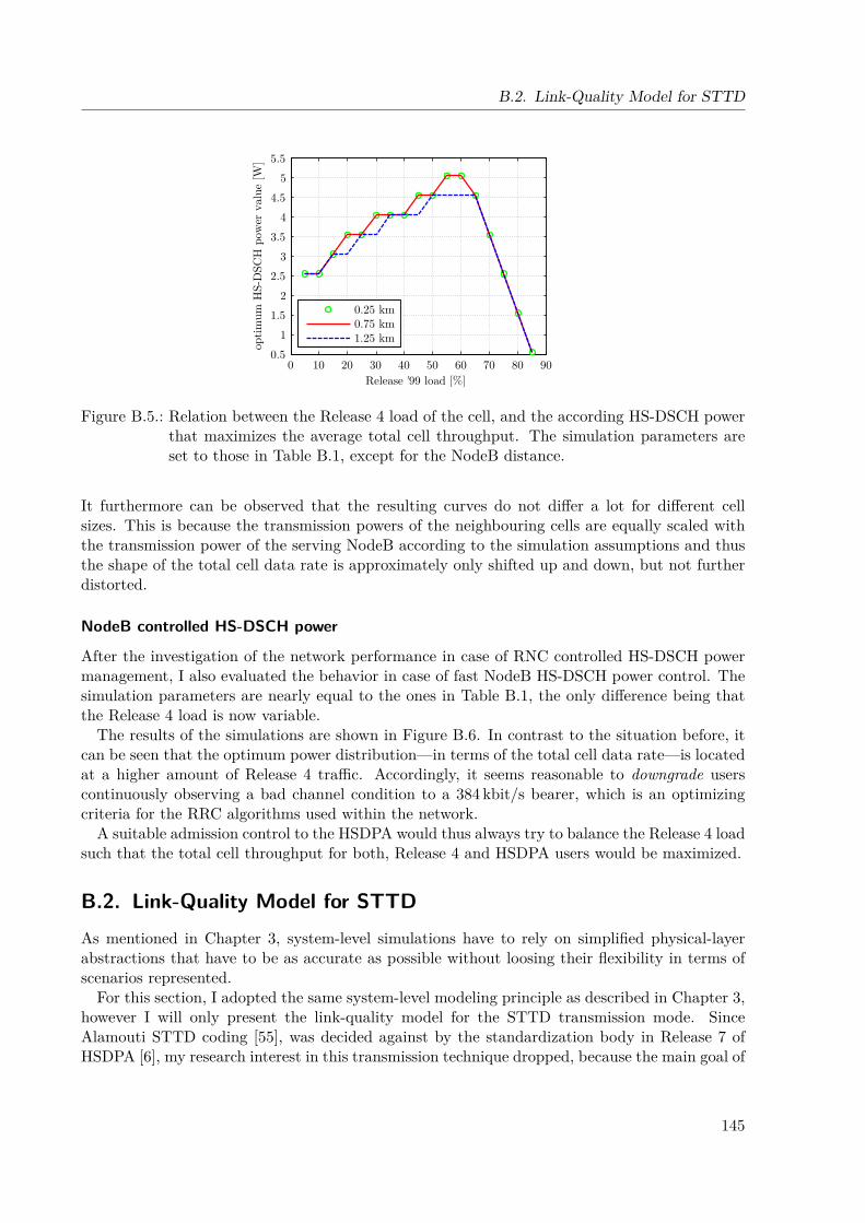
B.2. Link-Quality Model for STTD
0 10 20 30 40 50 60 70 80 900.5
1
1.5
2
2.5
3
3.5
4
4.5
5
5.5
Release '99 load [%]
optim
um H
S-D
SCH
pow
er v
alue
[W
]
0.25 km0.75 km1.25 km
Figure B.5.: Relation between the Release 4 load of the cell, and the according HS-DSCH powerthat maximizes the average total cell throughput. The simulation parameters areset to those in Table B.1, except for the NodeB distance.
It furthermore can be observed that the resulting curves do not differ a lot for different cellsizes. This is because the transmission powers of the neighbouring cells are equally scaled withthe transmission power of the serving NodeB according to the simulation assumptions and thusthe shape of the total cell data rate is approximately only shifted up and down, but not furtherdistorted.
NodeB controlled HS-DSCH power
After the investigation of the network performance in case of RNC controlled HS-DSCH powermanagement, I also evaluated the behavior in case of fast NodeB HS-DSCH power control. Thesimulation parameters are nearly equal to the ones in Table B.1, the only difference being thatthe Release 4 load is now variable.
The results of the simulations are shown in Figure B.6. In contrast to the situation before, itcan be seen that the optimum power distribution—in terms of the total cell data rate—is locatedat a higher amount of Release 4 traffic. Accordingly, it seems reasonable to downgrade userscontinuously observing a bad channel condition to a 384 kbit/s bearer, which is an optimizingcriteria for the RRC algorithms used within the network.
A suitable admission control to the HSDPA would thus always try to balance the Release 4 loadsuch that the total cell throughput for both, Release 4 and HSDPA users would be maximized.
B.2. Link-Quality Model for STTDAs mentioned in Chapter 3, system-level simulations have to rely on simplified physical-layerabstractions that have to be as accurate as possible without loosing their flexibility in terms ofscenarios represented.
For this section, I adopted the same system-level modeling principle as described in Chapter 3,however I will only present the link-quality model for the STTD transmission mode. SinceAlamouti STTD coding [55], was decided against by the standardization body in Release 7 ofHSDPA [6], my research interest in this transmission technique dropped, because the main goal of
145
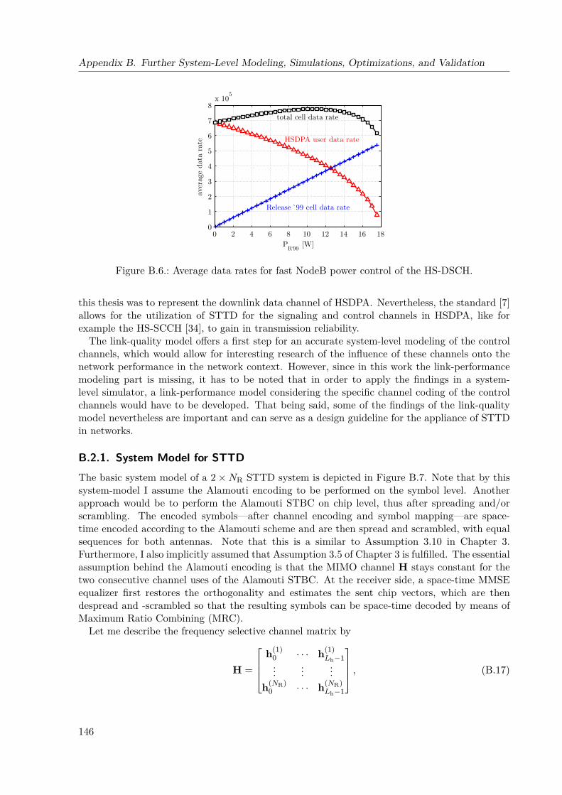
Appendix B. Further System-Level Modeling, Simulations, Optimizations, and Validation
0 2 4 6 8 10 12 14 16 180
1
2
3
4
5
6
7
8x 10
5
PR'99
[W]
aver
age
data
rat
e HSDPA user data rate
Release `99 cell data rate
total cell data rate
Figure B.6.: Average data rates for fast NodeB power control of the HS-DSCH.
this thesis was to represent the downlink data channel of HSDPA. Nevertheless, the standard [7]allows for the utilization of STTD for the signaling and control channels in HSDPA, like forexample the HS-SCCH [34], to gain in transmission reliability.
The link-quality model offers a first step for an accurate system-level modeling of the controlchannels, which would allow for interesting research of the influence of these channels onto thenetwork performance in the network context. However, since in this work the link-performancemodeling part is missing, it has to be noted that in order to apply the findings in a system-level simulator, a link-performance model considering the specific channel coding of the controlchannels would have to be developed. That being said, some of the findings of the link-qualitymodel nevertheless are important and can serve as a design guideline for the appliance of STTDin networks.
B.2.1. System Model for STTDThe basic system model of a 2×NR STTD system is depicted in Figure B.7. Note that by thissystem-model I assume the Alamouti encoding to be performed on the symbol level. Anotherapproach would be to perform the Alamouti STBC on chip level, thus after spreading and/orscrambling. The encoded symbols—after channel encoding and symbol mapping—are space-time encoded according to the Alamouti scheme and are then spread and scrambled, with equalsequences for both antennas. Note that this is a similar to Assumption 3.10 in Chapter 3.Furthermore, I also implicitly assumed that Assumption 3.5 of Chapter 3 is fulfilled. The essentialassumption behind the Alamouti encoding is that the MIMO channel H stays constant for thetwo consecutive channel uses of the Alamouti STBC. At the receiver side, a space-time MMSEequalizer first restores the orthogonality and estimates the sent chip vectors, which are thendespread and -scrambled so that the resulting symbols can be space-time decoded by means ofMaximum Ratio Combining (MRC).
Let me describe the frequency selective channel matrix by
H =
h(1)
0 · · · h(1)Lh−1
......
...h(NR)
0 · · · h(NR)Lh−1
, (B.17)
146
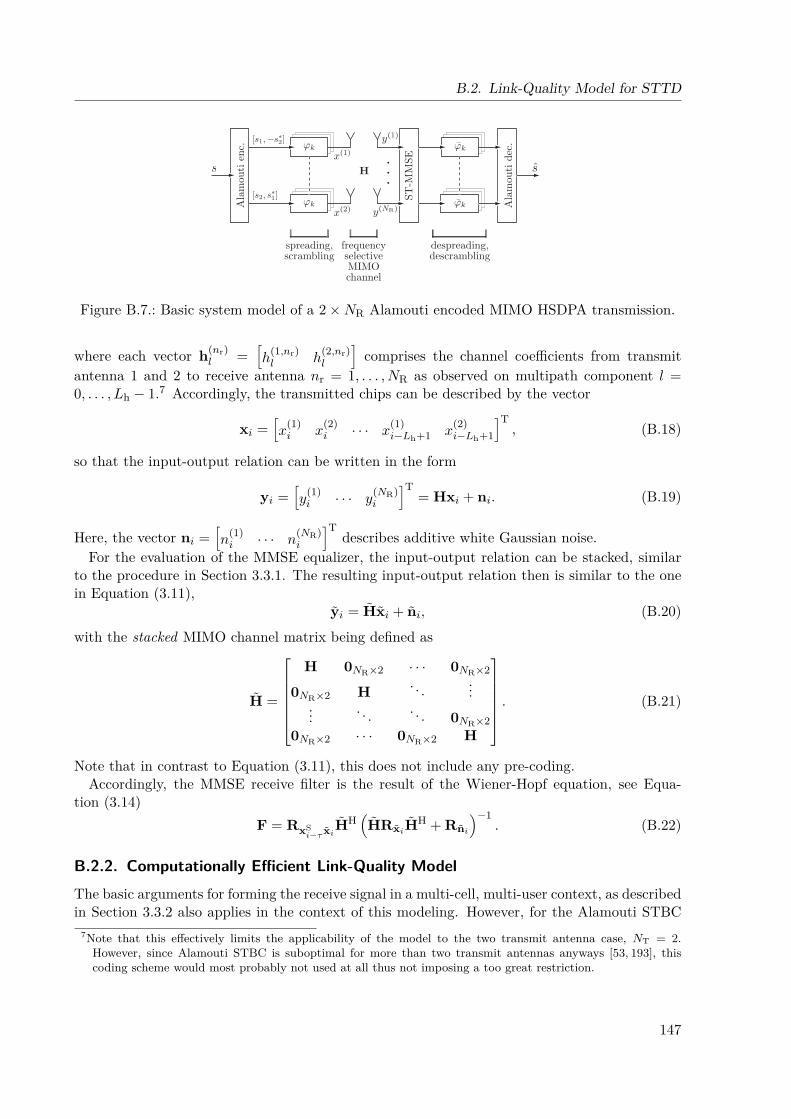
B.2. Link-Quality Model for STTD
Ala
mou
ti e
nc.
ST-M
MSE
H
spreading,scrambling
despreading,descrambling
frequencyselectiveMIMOchannel
Ala
mou
ti d
ec.
Figure B.7.: Basic system model of a 2×NR Alamouti encoded MIMO HSDPA transmission.
where each vector h(nr)l =
[h
(1,nr)l h
(2,nr)l
]comprises the channel coefficients from transmit
antenna 1 and 2 to receive antenna nr = 1, . . . , NR as observed on multipath component l =0, . . . , Lh − 1.7 Accordingly, the transmitted chips can be described by the vector
xi =[x
(1)i x
(2)i · · · x
(1)i−Lh+1 x
(2)i−Lh+1
]T, (B.18)
so that the input-output relation can be written in the form
yi =[y
(1)i · · · y
(NR)i
]T= Hxi + ni. (B.19)
Here, the vector ni =[n
(1)i · · · n
(NR)i
]Tdescribes additive white Gaussian noise.
For the evaluation of the MMSE equalizer, the input-output relation can be stacked, similarto the procedure in Section 3.3.1. The resulting input-output relation then is similar to the onein Equation (3.11),
yi = Hxi + ni, (B.20)
with the stacked MIMO channel matrix being defined as
H =
H 0NR×2 · · · 0NR×2
0NR×2 H . . . ...... . . . . . . 0NR×2
0NR×2 · · · 0NR×2 H
. (B.21)
Note that in contrast to Equation (3.11), this does not include any pre-coding.Accordingly, the MMSE receive filter is the result of the Wiener-Hopf equation, see Equa-
tion (3.14)F = RxS
i−τ xiHH(HRxiHH + Rni
)−1. (B.22)
B.2.2. Computationally Efficient Link-Quality ModelThe basic arguments for forming the receive signal in a multi-cell, multi-user context, as describedin Section 3.3.2 also applies in the context of this modeling. However, for the Alamouti STBC
7Note that this effectively limits the applicability of the model to the two transmit antenna case, NT = 2.However, since Alamouti STBC is suboptimal for more than two transmit antennas anyways [53, 193], thiscoding scheme would most probably not used at all thus not imposing a too great restriction.
147
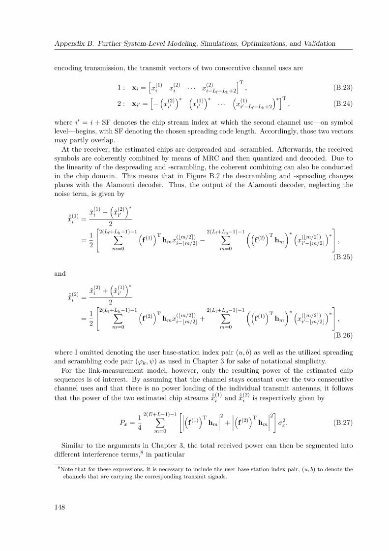
Appendix B. Further System-Level Modeling, Simulations, Optimizations, and Validation
encoding transmission, the transmit vectors of two consecutive channel uses are
1 : xi =[x
(1)i x
(2)i · · · x
(2)i−Lf−Lh+2
]T, (B.23)
2 : xi′ =[−(x
(2)i′
)∗ (x
(1)i′
)∗· · ·
(x
(1)i′−Lf−Lh+2
)∗]T, (B.24)
where i′ = i + SF denotes the chip stream index at which the second channel use—on symbollevel—begins, with SF denoting the chosen spreading code length. Accordingly, those two vectorsmay partly overlap.
At the receiver, the estimated chips are despreaded and -scrambled. Afterwards, the receivedsymbols are coherently combined by means of MRC and then quantized and decoded. Due tothe linearity of the despreading and -scrambling, the coherent combining can also be conductedin the chip domain. This means that in Figure B.7 the descrambling and -spreading changesplaces with the Alamouti decoder. Thus, the output of the Alamouti decoder, neglecting thenoise term, is given by
ˆx(1)i =
x(1)i −
(x
(2)i′
)∗2
= 12
2(Lf+Lh−1)−1∑m=0
(f (1)
)Thmx(bm/2e)
i−bm/2c −2(Lf+Lh−1)−1∑
m=0
((f (2)
)Thm)∗ (
x(bm/2e)i′−bm/2c
)∗ ,(B.25)
and
ˆx(2)i =
x(2)i +
(x
(1)i′
)∗2
= 12
2(Lf+Lh−1)−1∑m=0
(f (2)
)Thmx(bm/2e)
i−bm/2c +2(Lf+Lh−1)−1∑
m=0
((f (1)
)Thm)∗ (
x(bm/2e)i′−bm/2c
)∗ ,(B.26)
where I omitted denoting the user base-station index pair (u, b) as well as the utilized spreadingand scrambling code pair (ϕk, ψ) as used in Chapter 3 for sake of notational simplicity.
For the link-measurement model, however, only the resulting power of the estimated chipsequences is of interest. By assuming that the channel stays constant over the two consecutivechannel uses and that there is no power loading of the individual transmit antennas, it followsthat the power of the two estimated chip streams ˆx(1)
i and ˆx(2)i is respectively given by
Px = 14
2(E+L−1)−1∑m=0
[∣∣∣∣(f (1))T
hm∣∣∣∣2 +
∣∣∣∣(f (2))T
hm∣∣∣∣2]σ2x. (B.27)
Similar to the arguments in Chapter 3, the total received power can then be segmented intodifferent interference terms,8 in particular
8Note that for these expressions, it is necessary to include the user base-station index pair, (u, b) to denote thechannels that are carrying the corresponding transmit signals.
148
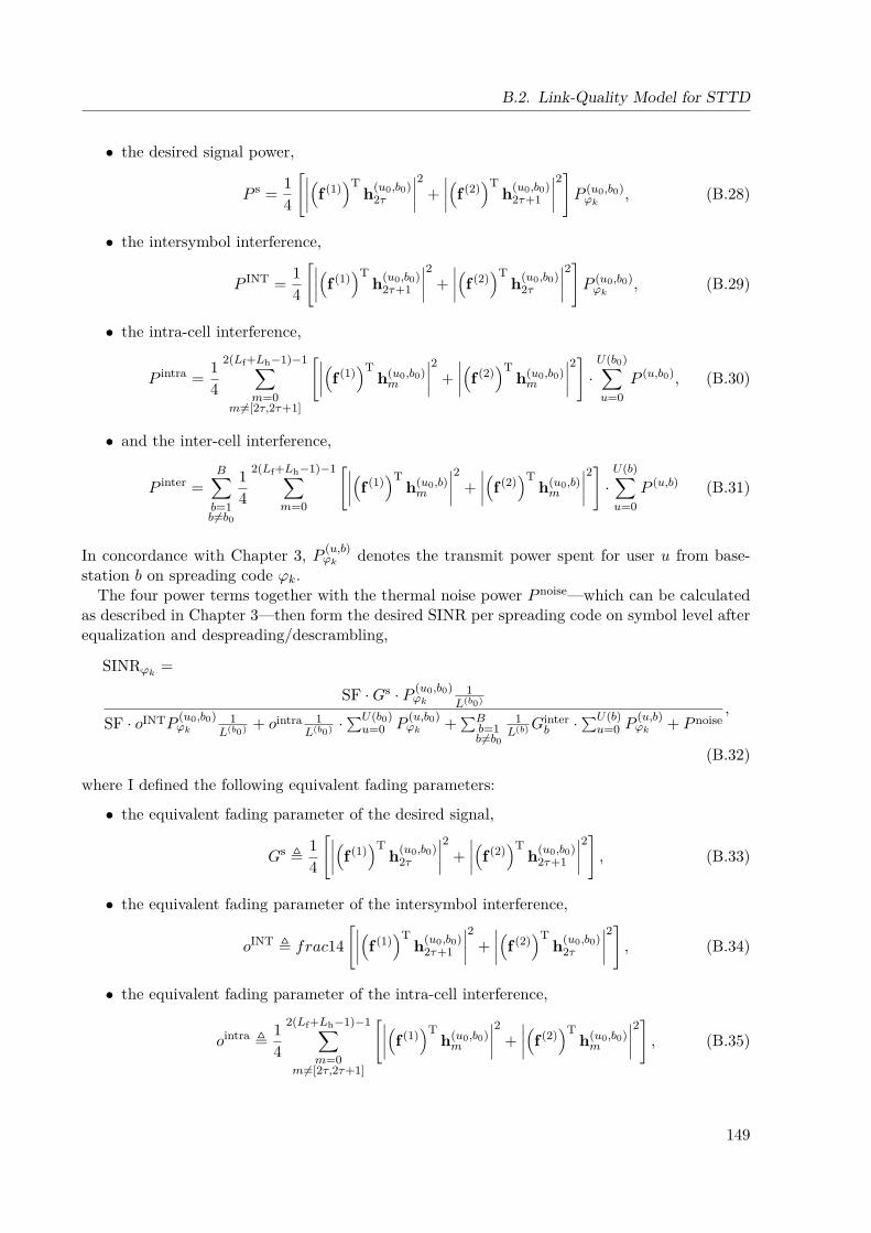
B.2. Link-Quality Model for STTD
• the desired signal power,
P s = 14
[∣∣∣∣(f (1))T
h(u0,b0)2τ
∣∣∣∣2 +∣∣∣∣(f (2)
)Th(u0,b0)
2τ+1
∣∣∣∣2]P (u0,b0)ϕk
, (B.28)
• the intersymbol interference,
P INT = 14
[∣∣∣∣(f (1))T
h(u0,b0)2τ+1
∣∣∣∣2 +∣∣∣∣(f (2)
)Th(u0,b0)
2τ
∣∣∣∣2]P (u0,b0)ϕk
, (B.29)
• the intra-cell interference,
P intra = 14
2(Lf+Lh−1)−1∑m=0
m6=[2τ,2τ+1]
[∣∣∣∣(f (1))T
h(u0,b0)m
∣∣∣∣2 +∣∣∣∣(f (2)
)Th(u0,b0)m
∣∣∣∣2]·U(b0)∑u=0
P (u,b0), (B.30)
• and the inter-cell interference,
P inter =B∑b=1b6=b0
14
2(Lf+Lh−1)−1∑m=0
[∣∣∣∣(f (1))T
h(u0,b)m
∣∣∣∣2 +∣∣∣∣(f (2)
)Th(u0,b)m
∣∣∣∣2]·U(b)∑u=0
P (u,b) (B.31)
In concordance with Chapter 3, P (u,b)ϕk denotes the transmit power spent for user u from base-
station b on spreading code ϕk.The four power terms together with the thermal noise power P noise—which can be calculated
as described in Chapter 3—then form the desired SINR per spreading code on symbol level afterequalization and despreading/descrambling,
SINRϕk =
SF ·Gs · P (u0,b0)ϕk
1L(b0)
SF · oINTP(u0,b0)ϕk
1L(b0) + ointra 1
L(b0) ·∑U(b0)u=0 P
(u,b0)ϕk +
∑Bb=1b 6=b0
1L(b)G
interb ·
∑U(b)u=0 P
(u,b)ϕk + P noise
,
(B.32)
where I defined the following equivalent fading parameters:
• the equivalent fading parameter of the desired signal,
Gs ,14
[∣∣∣∣(f (1))T
h(u0,b0)2τ
∣∣∣∣2 +∣∣∣∣(f (2)
)Th(u0,b0)
2τ+1
∣∣∣∣2], (B.33)
• the equivalent fading parameter of the intersymbol interference,
oINT , frac14[∣∣∣∣(f (1)
)Th(u0,b0)
2τ+1
∣∣∣∣2 +∣∣∣∣(f (2)
)Th(u0,b0)
2τ
∣∣∣∣2], (B.34)
• the equivalent fading parameter of the intra-cell interference,
ointra ,14
2(Lf+Lh−1)−1∑m=0
m 6=[2τ,2τ+1]
[∣∣∣∣(f (1))T
h(u0,b0)m
∣∣∣∣2 +∣∣∣∣(f (2)
)Th(u0,b0)m
∣∣∣∣2], (B.35)
149
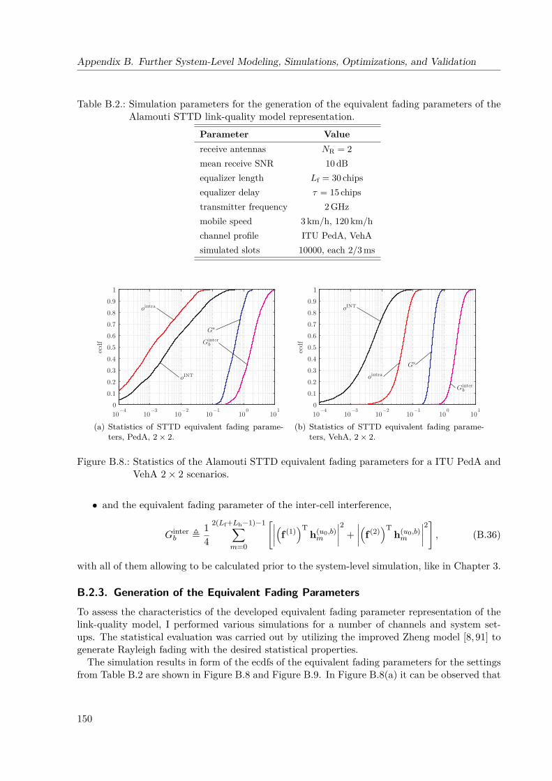
Appendix B. Further System-Level Modeling, Simulations, Optimizations, and Validation
Table B.2.: Simulation parameters for the generation of the equivalent fading parameters of theAlamouti STTD link-quality model representation.
Parameter Valuereceive antennas NR = 2mean receive SNR 10 dBequalizer length Lf = 30 chipsequalizer delay τ = 15 chipstransmitter frequency 2 GHzmobile speed 3 km/h, 120 km/hchannel profile ITU PedA, VehAsimulated slots 10000, each 2/3 ms
10−4
10−3
10−2
10−1
100
101
0
0.1
0.2
0.3
0.4
0.5
0.6
0.7
0.8
0.9
1
ecdf
(a) Statistics of STTD equivalent fading parame-ters, PedA, 2× 2.
10−4
10−3
10−2
10−1
100
101
0
0.1
0.2
0.3
0.4
0.5
0.6
0.7
0.8
0.9
1ecdf
(b) Statistics of STTD equivalent fading parame-ters, VehA, 2× 2.
Figure B.8.: Statistics of the Alamouti STTD equivalent fading parameters for a ITU PedA andVehA 2× 2 scenarios.
• and the equivalent fading parameter of the inter-cell interference,
Ginterb ,
14
2(Lf+Lh−1)−1∑m=0
[∣∣∣∣(f (1))T
h(u0,b)m
∣∣∣∣2 +∣∣∣∣(f (2)
)Th(u0,b)m
∣∣∣∣2], (B.36)
with all of them allowing to be calculated prior to the system-level simulation, like in Chapter 3.
B.2.3. Generation of the Equivalent Fading ParametersTo assess the characteristics of the developed equivalent fading parameter representation of thelink-quality model, I performed various simulations for a number of channels and system set-ups. The statistical evaluation was carried out by utilizing the improved Zheng model [8, 91] togenerate Rayleigh fading with the desired statistical properties.
The simulation results in form of the ecdfs of the equivalent fading parameters for the settingsfrom Table B.2 are shown in Figure B.8 and Figure B.9. In Figure B.8(a) it can be observed that
150
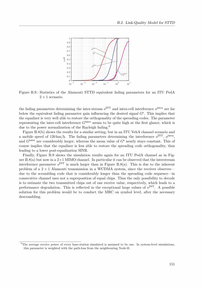
B.2. Link-Quality Model for STTD
10−4
10−3
10−2
10−1
100
101
0
0.1
0.2
0.3
0.4
0.5
0.6
0.7
0.8
0.9
1
ecdf
Figure B.9.: Statistics of the Alamouti STTD equivalent fading parameters for an ITU PedA2× 1 scenario.
the fading parameters determining the inter-stream oINT and intra-cell interference ointra are farbelow the equivalent fading parameter gain influencing the desired signal Gs. This implies thatthe equalizer is very well able to restore the orthogonality of the spreading codes. The parameterrepresenting the inter-cell interference Ginter seems to be quite high at the first glance, which isdue to the power normalization of the Rayleigh fading.9
Figure B.8(b) shows the results for a similar setting, but in an ITU VehA channel scenario anda mobile speed of 120 km/h. The fading parameters determining the interference oINT, ointra,and Ginter are considerably larger, whereas the mean value of Gs nearly stays constant. This ofcourse implies that the equalizer is less able to restore the spreading code orthogonality, thusleading to a lower post-equalization SINR.
Finally, Figure B.9 shows the simulation results again for an ITU PedA channel as in Fig-ure B.8(a) but now in a 2×1 MIMO channel. In particular it can be observed that the interstreaminterference parameter oINT is much larger than in Figure B.8(a). This is due to the inherentproblem of a 2 × 1 Alamouti transmission in a WCDMA system, since the receiver observes—due to the scrambling code that is considerably longer than the spreading code sequence—inconsecutive channel uses not a superposition of equal chips. Thus the only possibility to decodeis to estimate the two transmitted chips out of one receive value, respectively, which leads to aperformance degradation. This is reflected in the exceptional large values of oINT. A possiblesolution for this problem would be to conduct the MRC on symbol level, after the necessarydescrambling.
9The average receive power of every base-station simulated is assumed to be one. In system-level simulations,this parameter is weighted with the path-loss from the neighbouring Node-B.
151


List of Abbreviations
3GPP 3rd Generation Partnership ProjectACK ACKnowledgedAMC Adaptive Modulation and CodingAWGN Additive White Gaussian NoiseBICM Bit-Interleaved Coded ModulationBLER BLock Error RatioCA Content-AwareCDMA Code-Division Multiple AccessCL Closed LoopCOST European COoperation in the field of Scientific and Technical researchCPICH Common Pilot CHannelCQI Channel Quality IndicatorCRC Cyclic Redundancy CheckCSI Channel State InformationDCCH Dedicated Control CHannelDCH Dedicated CHannelDiffServ Differentiate ServiceDoF Degrees of FreedomDPC Dirty Paper CodingDPCCH Dedicated Physical Control CHannelDPDCH Dedicated Physical Data CHannelDS Double-StreamDSTTD-SGRC Double Space-Time Transmit Diversity with Sub-Group Rate ControlDTCH Dedicated Traffic CHannelD-TxAA Double Transmit Antenna Arrayecdf empirical cumulative distribution functionEDGE Enhanced Data Rates for Global system for mobile communications EvolutionEESM Exponential Effective Signal to Interference and Noise Ratio Mappingepdf empirical probability density functionFBI FeedBack InformationFDD Frequency Division DuplexGGSN Gateway-General packet radio service Support NodeGOF Goodness Of Fit
153
Appendix B. Further System-Level Modeling, Simulations, Optimizations, and Validation
GOP Group Of PicturesGPRS General Packet Radio ServiceGSM Global System for Mobile communicationsHARQ Hybrid Automatic Repeat reQuestHSDPA High-Speed Downlink Packet AccessHS-DPCCH High-Speed Dedicated Physical Control CHannelHS-DSCH High-Speed Downlink Shared CHannelHSPA High-Speed Packet AccessHS-PDSCH High-Speed Physical Downlink Shared CHannelHS-SCCH High-Speed Shared Control CHannelHSUPA High-Speed Uplink Packet AccessIC Interference CancellationIDE Integrated Development EnvironmentIP Internet ProtocolIR Incremental RedundancyISI Inter-Symbol InterferenceISO International Standard OrganizationITU International Telecommunication UnionLS Least SquaresLTE Long Term EvolutionMAC Medium Access ControlMAC-d Medium Access Control dedicatedMAC-hs Medium Access Control for High-Speed Downlink Packet Accessmax C/I Maximum Carrier-to-Interference RatioMB MacroBlockMI Mutual InformationMIESM Mutual Information Effective Signal to Interference and Noise Ratio MappingMIMO Multiple-Input Multiple-OutputMISO Multiple-Input Single-OutputML Maximum LikelihoodMMSE Minimum Mean Squared ErrorMoRSE Mobile Radio Simulation EnvironmentMPEG Moving Picture Expert GroupMRC Maximum Ratio CombiningMSE Mean Squared ErrorMTU Maximum Transfer UnitMU Multi-UserMVU Minimum Variance Unbiased
154

B.2. Link-Quality Model for STTD
NACK Non-ACKnowledgedNAL Network Abstract LayerNBAP NodeB Application PartNDI New Data IndicatorN-SAW N Stop And WaitNSN Nokia Siemens NetworksOFDMA Orthogonal Frequency-Division Multiple AccessOSI Open Systems InterconnectionPARC Per-Antenna Rate ControlPCI Precoding Control InformationPDCP Packet Data Convergence Protocolpdf probability density functionPDP Packet Data ProtocolPDU Packet Data UnitPedA Pedestrian APedB Pedestrian BPER Packet Error RatioPF Proportional FairPN Pseudo NoisePSD Power Spectral DensityPSNR Peak Signal to Noise RatioQAM Quadrature Amplitude ModulationQCIF Quarter Common Intermediate FormatQoE Quality of ExperienceQoS Quality of ServiceRAN Radio Access NetworkRF Radio FrequencyRLC Radio Link ControlRMS Root Mean SquareRNC Radio Network ControllerRR Round RobinRRC Radio Resource ControlRRM Radio Resource ManagementRTP Real-time Transport ProtocolRV Redundancy VersionSAE System Architecture EvolutionSCM Spatial Channel ModelSCME Spatial Channel Model Extended
155
Appendix B. Further System-Level Modeling, Simulations, Optimizations, and Validation
SDMA Spatial Division Multiple AccessSDU Service Data UnitSGSN Serving-General packet radio service Support NodeSIC Successive Interference CancellationSID Size Index IdentifierSIMO Single-Input Multiple-OutputSINR Signal-to-Interference-and-Noise RatioSISO Single-Input Single-OutputSNR Signal-to-Noise RatioSQP Sequential Quadratic ProgrammingSS Single-StreamSTBC Space-Time Block CodeSTTD Space-Time Transmit DiversitySU Single-UserSVD Singular Value DecompositionTBS Transport Block SizeTDD Time Division DuplexTFC Transport Format CombinationTFCI Transport-Format Combination IndicatorTFT Traffic Flow TemplateTOS Type Of ServiceTPC Transmit Power-ControlTrCH Transport CHannelTSN Transmission Sequence NumberTTI Transmission Time IntervalTxAA Transmit Antenna ArrayUDP User Datagram ProtocolUE User EquipmentUMTS Universal Mobile Telecommunications SystemUTRAN Universal mobile telecommunications system Terrestrial Radio Access NetworkV-BLAST Vertical Bell Laboratories Layered Space-TimeVCEG Video Coding Expert GroupVCL Video Coding LayerVehA Vehicular AVHSIC Very High Speed Integrated CircuitsVoIP Voice over IPWCDMA Wideband Code-Division Multiple Access
156
List of Symbols
This list of symbols generally holds throughout the thesis. However, if clearly stated in the text,it may had been necessary to redefine one or multiple of these, so the meaning should always bechecked in concordance with the corresponding section.
α power coefficientA symbol alphabetb base-station/sector indexB total number of base-stations/sectorsBf bandwidthβ link-performance model tuning parameter vectorc(F) feedback CQIcr relative complexityc(T) transmit CQIC set of complex numbersd distance between UE and target NodeBEc average chip energyf receive filterF space-time MMSE equalizerfother other user interference fractionfself self interference fractionϕ spreading codeΦ spreading code setGintern,b inter-cell interference fading parameter
Gsn fading parameter of desired signal
h scaler complex channel coefficienth stacked equivalent MIMO channel columnH MIMO channelHw pre-coded equivalent MIMO channelHw stacked equivalent MIMO channel
157
Appendix B. Further System-Level Modeling, Simulations, Optimizations, and Validation
ˆHw estimated equivalent MIMO channeli discrete time indexIoc total white noise interference PSD at UEIor total transmit PSD at NodeBk spreading code indexL macro-scale and shadow fading path-lossLf equalizer lengthLh maximum channel delayλm macro-scale path-lossλs shadow fading path-lossm column indexn stream indexn noiseN0 noise PSDnr receive antenna indexNR total number of receive antennasNS number of spatial streamsnt transmit antenna indexNT total number of transmit antennasN set of integersoBFn fading parameter of pre-coding effectoINTn inter-stream fading parameterointran intra-cell interference fading parameter
Ω set of pre-coding weightsP pre-coding stateψ scrambling codeR raterc effective coderateR set of real numberss modulated symbolSF spreading factorσ2
n noise covariance
158
B.2. Link-Quality Model for STTD
T evaluated throughputTc chip durationτ filter delayϑ fairness coefficientT transport format mappingu user indexU total number of usersu(s) scheduled userν content priority indicatorw pre-coding weightW pre-coding matrixx transmit signaly receive signal
159


Bibliography
[1] Y. Li and J. I. Agbinya, “Emerging markets and benefits of fixed to wireless substitutionin africa,” in Proc. IEEE International Conference on Mobile Business (ICMB), Jul. 2005,pp. 605–609.
[2] M. Reardon. (2009, Apr.) CEOs see wireless as answer to economic crisis. [Online]. Avail-able: www.cnn.com/2009/TECH/biztech/04/02/wireless.might.solve.economic.crisis/
[3] H. Holma and A. Toskala, WCDMA for UMTS – Radio Access For Third GenerationMobile Communications, 3rd ed. John Wiley & Sons, Ltd, 2005.
[4] G. J. Foschini, “Layered space-time architecture for wireless communication in a fadingenvironment when using multiple antennas,” Bell Labs Technical Journal, vol. 1, no. 2, pp.41–59, 1996.
[5] E. Dahlman, S. Parkvall, J. Skold, and P. Beming, 3G Evolution: HSDPA and LTE forMobile Broadband. Academic Press, Jul. 2007.
[6] Technical Specification Group Radio Access Network, “Multiple-input multiple-outputUTRA,” 3rd Generation Partnership Project (3GPP), Tech. Rep. TR 25.876 Version 7.0.0,Mar. 2007.
[7] ——, “Physical layer procedures (FDD),” 3rd Generation Partnership Project (3GPP),Tech. Rep. TS 25.214 Version 7.4.0, Mar. 2007.
[8] Y. Zheng and C. Xiao, “Simulation models with correct statistical properties for rayleighfading channels,” IEEE Transactions on Communications, vol. 51, no. 6, pp. 920–928, Jun.2003.
[9] Technical Specification Group Radio Access Network, “Evolved universal terrestrial radioaccess (E-UTRA); LTE physical layer – general description,” 3rd Generation PartnershipProject (3GPP), Tech. Rep. TS 36.201 Version 8.3.0, Mar. 2009.
[10] (2009, May) Symena GmbH. [Online]. Available: www.symena.com
[11] S. Shakkottai, T. S. Rappaport, and P. C. Karlsson, “Cross-layer design for wireless net-works,” IEEE Communications Magazine, vol. 41, no. 10, pp. 74–80, Oct. 2003.
[12] M. Wrulich, C. Mecklenbrauker, J. Wehinger, S. Eder, and I. Kambourov, “Upgradingmethodology for MIMO system-level simulations,” Telecommunications Research CenterVienna (ftw.), project report C10, 2007.
[13] M. Wrulich, S. Eder, I. Viering, and M. Rupp, “Efficient link-to-system level model forMIMO HSDPA,” in Proc. IEEE 4th Broadband Wireless Access Workshop, 2008.
161
Bibliography
[14] M. Wrulich and M. Rupp, “Computationally efficient MIMO HSDPA system-level model-ing,” EURASIP Journal on Wireless Communications and Networking, 2009.
[15] ——, “Efficient link measurement model for system level simulations of Alamouti encodedMIMO HSDPA transmissions,” in Proc. ITG International Workshop on Smart Antennas(WSA), Darmstadt, Germany, Feb. 2008.
[16] C. Mehlfuhrer, S. Caban, M. Wrulich, and M. Rupp, “Joint throughput optimized CQIand precoding weight calculation for MIMO HSDPA,” in Proc. 42nd Asilomar Conferenceon Signals, Systems and Computers, Oct. 2008.
[17] M. Wrulich and C. Reyes, “Upgrading methodology for MIMO system-level simulations,”Telecommunications Research Center Vienna (ftw.), project report C12, 2008.
[18] G. Lilley, M. Wrulich, and M. Rupp, “Network based stream-number decision for MIMOHSDPA,” in Proc. ITG International Workshop on Smart Antennas (WSA), Feb. 2009.
[19] L. Superiori, M. Wrulich, P. Svoboda, M. Rupp, J. Fabini, W. Karner, and M. Steinbauer,“Content-aware scheduling for video streaming over HSDPA networks,” in Proc. IEEESecond International Workshop on Cross-Layer Design, 2009.
[20] L. Superiori, M. Wrulich, P. Svoboda, and M. Rupp, “Cross-layer optimization of videoservices over HSDPA networks,” in Proc. ICST International Conference on MobileLightweight Wireless Systems, 2009.
[21] A. Mateu-Torello, “CPICH power optimization for MIMO HSDPA,” Master’s thesis, Vi-enna University of Technology, Mar. 2009.
[22] M. Wrulich, C. Mehlfuhrer, and M. Rupp, “Interference aware MMSE equalization forMIMO TxAA,” in Proc. IEEE 3rd International Symposium on Communications, Controland Signal Processing (ISCCSP), 2008, pp. 1585–1589.
[23] C. Mehlfuhrer, M. Wrulich, and M. Rupp, “Intra-cell interference aware equalization forTxAA HSDPA,” in Proc. IEEE 3rd International Symposium on Wireless Pervasive Com-puting, 2008, pp. 406–409.
[24] M. Wrulich, C. Mehlfuhrer, and M. Rupp, Handbook of HSDPA/HSUPA Technology. CRCPress, 2009, ch. Advanced Receivers for MIMO HSDPA, in print preparation.
[25] ——, “Managing the interference structure of MIMO HSDPA: A multi-user interferenceaware MMSE receiver with moderate complexity,” 2009, submitted to IEEE Transactionson Wireless Communications.
[26] M. Wrulich, W. Weiler, and M.Rupp, “HSDPA performance in a mixed traffic network,”in Proc. IEEE Vehicular Technology Conference Spring (VTC), May 2008, pp. 2056–2060.
[27] P. Svoboda, W. Karner, and M. Rupp, “Traffic analysis and modeling for world of warcraft,”in Proc. IEEE International Conference on Communications (ICC), 2007, pp. 1612–1617.
[28] Commission of the European Communities, “Progress report on the single europeanelectronic communications market (14th report),” Commission of the EuropeanCommunities, Tech. Rep. SEC (2009) 376, 2008. [Online]. Available: http://eur-lex.europa.eu/LexUriServ/LexUriServ.do?uri=COM:2009:0140:FIN:EN:PDF
162
Bibliography
[29] ——, “Towards a single european telecoms market – focus on Austria,” Commission of theEuropean Communities, Tech. Rep., Mar. 2009. [Online]. Available: http://ex.europa.eu/information society/doc/factsheets/14thimplementation/14th-progress-report-at-final.pdf
[30] H. Wittig, “The power of mobile broadband – implications for european telcos and equip-ment vendors,” J.P. Morgan Securities Ltd., Tech. Rep., May 2008.
[31] A. Grinschgl and G. Serentschy, “Kommunikationsbericht 2007,” Rundfunk und TelekomRegulierungs-GmbH, Tech. Rep., 2007. [Online]. Available: http://www.rtr.at/de/komp/KBericht2007/K-Bericht 2007.pdf
[32] Technical Specification Group Radio Access Network, “UTRA high speed downlink packetaccess (HSDPA); overall description; stage 2,” 3rd Generation Partnership Project (3GPP),Tech. Rep. TS 25.308 Version 5.0.0, Sep. 2001.
[33] H. Holma and A. Toskala, HSDPA/HSUPA for UMTS: High Speed Radio Access for MobileCommunications. John Wiley & Sons, Ltd., 2006, ISBN 0-470-01884-4.
[34] Technical Specification Group Radio Access Network, “Physical channels and mapping oftransport channels onto physical channels (FDD),” 3rd Generation Partnership Project(3GPP), Tech. Rep. TS 25.211, Version 8.4.0, Mar. 2009.
[35] ——, “Multiplexing and channel coding (FDD),” 3rd Generation Partnership Project(3GPP), Tech. Rep. TS 25.212 Version 8.5.0, Mar. 2009.
[36] E. Malkamaki, D. Mathew, and S. Hamalainen, “Performance of hybrid ARQ techniquesfor WCDMA high data rates,” Proc. IEEE 53rd Vehicular Technology Conference Spring(VTC), vol. 4, pp. 2720–2724, 2001.
[37] P. Frenger, S. Parkvall, and E. Dahlman, “Performance comparison of HARQ with chasecombining and incremental redundancy for HSDPA,” Proc. VTS IEEE 54th VehicularTechnology Conference Fall (VTC), vol. 3, pp. 1829–1833, 2001.
[38] P. Wu and N. Jindal, “Performance of hybrid-ARQ in block-fading channels: A fixed outageprobability analysis,” Nov. 2008, submitted to IEEE Transactions on Wireless Communi-cations.
[39] Members of TSG-RAN Working Group 4, “Revised HSDPA CQI proposal,” 3GPP, Tech.Rep. R4-020612, 2002.
[40] Technical Specification Group Radio Access Network, “User equipment (UE) radio trans-mission and reception (FDD),” 3rd Generation Partnership Project (3GPP), Tech. Rep.TS 25.101, Version 8.6.0, Mar. 2009.
[41] ——, “Medium access control (MAC) protocol specification,” 3rd Generation PartnershipProject (3GPP), Tech. Rep. TS 25.321 Version 7.0.0, Mar. 2006.
[42] S. Blomeier, HSDPA - Design Details & System Engineering. INACON, 2006, ISBN978-3-936273-42-7.
[43] Technical Specification Group Radio Access Network, “Radio link control (RLC) protocolspecification,” 3rd Generation Partnership Project (3GPP), Tech. Rep. TS 25.322 Version8.4.0, Mar. 2009.
163
Bibliography
[44] K. Pedersen and P. Michaelsen, “Algorithms and performance results for dynamic HSDPAresource allocation,” in Proc. IEEE 64th Vehicular Technology Conference (VTC), Sep.2006, pp. 1–5.
[45] I. de Bruin, G. Heijenk, M. El Zarki, and L. Zan, “Fair channel-dependent scheduling inCDMA systems,” in Proc. IST Mobile and Wireless Communications Summit, Jun. 2003,pp. 737–741.
[46] M. H. Ahmed, H. Yanikomeroglu, and S. Mahmoud, “Fairness enhancement of link adap-tation techniques in wireless access networks,” in Proc. IEEE Vehicular Technology Con-ference Fall (VTC), vol. 3, Oct. 2003, pp. 1554–1557.
[47] C. Wengerter, J. Ohlhorst, and A. Golitschek Edler von Elbwart, “Fairness and throughputanalysis for generalized proportional fair frequency scheduling in OFDMA,” in Proc. IEEE61st Vehicular Technology Conference (VTC) Spring, vol. 3, Jun. 2005, pp. 1903–1907.
[48] I. E. Telatar, “Capacity of multi-antenna gaussian channels,” European Trans. on Telecom.,vol. 10, pp. 585–595, 1999.
[49] A. Paulraj, R. Nabar, and D. Gore, Introduction to Space-Time Wireless Communications.Cambridge University Press, 2003, ISBN 0521826152.
[50] S. A. Jafar and M. J. Fakhereddin, “Degrees of freedom for the MIMO interference channel,”IEEE Transactions on Information Theory, vol. 53, no. 7, pp. 2637–2642, Jul. 2007.
[51] D. Gesbert, M. Shafi, D. Shiu, P. J. Smith, and A. Naguib, “From theory to practice: Anoverview of MIMO space-time coded wireless systems,” IEEE Journal on Selected Areas inCommunications, vol. 21, no. 3, pp. 281–302, Apr. 2003.
[52] V. Tarokh, N. Seshadri, and A. R. Calderbank, “Space-time codes for high data ratewireless communication: Performance criterion and code construction,” IEEE Transactionson Information Theory, vol. 44, no. 2, pp. 744–765, Mar. 1998.
[53] M. Wrulich, “Capacity analysis of MIMO systems,” Master’s thesis, Vienna University ofTechnology, Mar. 2006.
[54] L. Zheng and D. N. C. Tse, “Diversity and multiplexing: A fundamental tradeoff inmultiple-antenna channels,” IEEE Transactions on Information Theory, vol. 49, no. 5,pp. 1073–1096, May 2003.
[55] S. Alamouti, “A simple transmit diversity technique for wireless communications,” IEEEJournal on Selected Areas in Communications, vol. 16, no. 8, pp. 1451–1458, Oct. 1998.
[56] A. Lozano and N. Jindal, “Transmit diversity v. spatial multiplexing in modern MIMOsystems,” Nov. 2008, submitted to IEEE Transactions on Wireless Communications.
[57] J.-C. Belfiore, G. Rekaya, and E. Viterbo, “The golden code: A 2x2 full-rate space-timecode with nonvanishing determinants,” IEEE Transactions on Information Theory, vol. 51,no. 4, pp. 1432–1426, Apr. 2005.
[58] H. Bolcskei, D. Gesbert, C. B. Papadias, and A.-J. Van der Veen, Eds., Space-Time WirelessSystems – From Array Processing to MIMO Communications. Cambridge University Press,2006, ISBN 978-0-521-85105-3.
164
Bibliography
[59] Motorola, “MIMO evaluation proposal,” 3rd Generation Partnership Project (3GPP), Tech.Rep. TSG R1 #44 060615, Feb. 2006.
[60] Q. Spencer, C. Peel, A. Swindlehurst, and M. Haardt, “An introduction to the multi-userMIMO downlink,” IEEE Communications Magazine, vol. 42, no. 10, pp. 60–67, Oct. 2004.
[61] D. Gesbert, M. Kountouris, R. Heath, C.-B. Chae, and T. Salzer, “Shifting the MIMOparadigm,” IEEE Signal Processing Magazine, vol. 24, no. 5, pp. 36–46, Sep. 2007.
[62] H. Holma, A. Toskala, K. Ranta-aho, and J. Pirskanen, “High-speed packet access evolutionin 3GPP release 7,” IEEE Communications Magazine, vol. 45, no. 12, pp. 29–35, Dec. 2007.
[63] L. Haring, B. Chalise, and A. Czylwik, “Dynamic system level simulations of downlinkbeamforming for UMTS FDD,” in Proc. IEEE Global Telecommunications Conference(GLOBECOM), vol. 1, 2003, pp. 492–496.
[64] A. Czylwik and A. Dekorsy, “System-level performance of antenna arrays in CDMA-basedcellular mobile radio systems,” EURASIP J. Appl. Signal Proc., no. 9, pp. 1308–1320, 2004.
[65] K. Peppas, A. Alexiou, F. Lazarakis, and T. Al-Gizawi, “Performance evaluation at thesystem level of reconfigurable space-time coding techniques for HSDPA,” EURASIP J.Appl. Signal Proc., no. 11, pp. 1656–1667, 2005.
[66] T. Nihtila and V. Haikola, “HSDPA MIMO system performance in macro cell network,”in Proc. IEEE Sarnoff Symposium, 2008, pp. 1–4.
[67] K. I. Pedersen, T. F. Lootsma, M. Stottrup, F. Frederiksen, T. Kolding, and P. E. Mo-gensen, “Network performance of mixed traffic on high speed downlink packet access anddedicated channels in WCDMA,” in Proc. IEEE 60th Vehicular Technology Conference(VTC), vol. 6, 2004, pp. 4496–4500.
[68] P. Sai A and C. Furse, “System level analysis of noise and interference analysis for MIMOsystem,” in Proc. IEEE Antennas and Propagation Society International Symposium (AP-S), 2008, pp. 1–4.
[69] P. Gkonis, D. Kaklamani, and G. Tsoulos, “Capacity of WCDMA multicellular networksunder different radio resource management strategies,” in Proc. 3rd International Sympo-sium on Wireless Pervasive Computing (ISWPC), 2008, pp. 60–64.
[70] M. Castaneda, M. Ivrlac, J. Nossek, I. Viering, and A. Klein, “On downlink intercell inter-ference in a cellular system,” in Proc. IEEE 18th International Symposium on Personal,Indoor and Mobile Radio Communications (PIMRC), 2007, pp. 1–5.
[71] K. Peppas, T. Al-Gizawi, F. Lazarakis, D. Axiotis, A. Moussa, and A. Alexiou, “Systemlevel evaluation of reconfigurable MIMO techniques enhancements for HSDPA,” in Proc.IEEE Global Telecommunications Conference (GLOBECOM), vol. 5, 2004, pp. 2869–2873.
[72] A. Pollard and M. Heikkila, “A system level evaluation of multiple antenna schemes for highspeed downlink packet access,” in Proc. IEEE 15th International Symposium on Personal,Indoor and Mobile Radio Communications (PIMRC), vol. 3, 2004, pp. 1732–1735.
165
Bibliography
[73] C. Shuping, L. Huibinu, Z. Dong, and K. Asimakis, “Generalized scheduler providing mul-timedia services over HSDPA,” in Proc. IEEE International Conference on Multimedia andExpo, 2007, pp. 927–930.
[74] D. Skoutas, D. Komnakos, D. Vouyioukas, and A. Rouskas, “Enhanced dedicated channelscheduling optimization in WCDMA,” in Proc. 14th European Wireless Conference (EW),2008, pp. 1–5.
[75] D. Staehle and A. Mader, “A model for time-efficient HSDPA simulations,” in Proc. IEEE66th Vehicular Technology Conference Fall (VTC), 2007, pp. 819–823.
[76] D. Moltchanov, Y. Koucheryavy, and J. Harju, Wired/Wireless Internet Communica-tions, ser. Lecture Notes in Computer Science. Springer Berlin / Heidelberg, 2005, vol.3510/2005, ch. Simple, Accurate and Computationally Efficient Wireless Channel ModelingAlgorithm, pp. 234–245, ISBN 978-3-540-25899-5.
[77] ——, “Cross-layer modeling of wireless channels for data-link and IP layer performanceevaluation,” ELSEVIER Computer Communications, no. 29, pp. 827–841, 2006.
[78] A. Seeger, M. Sikora, and A. Klein, “Variable orthogonality factor: A simple interfacebetween link and system level simulation for high speed downlink packet access,” in Proc.IEEE 58th Vehicular Technology Conference Fall (VTC), Sep. 2003, pp. 2531–2534.
[79] S. W. Golomb, “Mathematical models – uses and limitations,” Simulation, vol. 4, no. 14,pp. 197–198, 1970.
[80] Members of WINNER, “Assessment of advanced beamforming and MIMO technologies,”WINNER, Tech. Rep. IST-2003-507581 D2.7 v1.0, 2003.
[81] S. Hamalainen, H. Holma, and K. Sipila, “Advanced WCDMA radio network simulator,”in Proc. IEEE International Symposium on Personal, Indoor and Mobile Radio Conference(PIMRC), Sep. 1999, pp. 951–955.
[82] B. Sklar, “Rayleigh fading channels in mobile digital communication systems. I. character-ization,” IEEE Communications Magazine, vol. 35, no. 9, pp. 136–146, Sep. 1997.
[83] S. Hamalainen, P. Slanina, M. Hartman, A. Lappetelainen, H. Holma, and O. Salonaho,“A novel interface between link and system level simulations,” in Proc. ACTS Summit,Oct. 1997, pp. 509–604.
[84] K. Brueninghaus, D. Astely, T. Salzer, S. Visuri, A. Alexiou, S. Karger, and G. A. Seraji,“Link performance models for system level simulations of broadband radio access systems,”in Proc. IEEE 16th International Symposium on Personal, Indoor and Mobile Radio Com-munications (PIMRC 2005), vol. 4, Sep. 2005, pp. 2306–2311.
[85] T. Nihtila, J. Kurjenniemi, and E. Virtej, “System level analysis of interference awareLMMSE chip equalization in HSDPA network,” in Proc. IEEE 12th Symposium on Com-puters and Communications (ISCC), 2007, pp. 133–138.
[86] J. Mirkovic, G. Orfanos, and H.-J. Reumerman, “MIMO link modeling for system levelsimulations,” in Proc. IEEE 17th International Symposium on Personal, Indoor and MobileRadio Communications (PIMRC), 2006, pp. 1–6.
166
Bibliography
[87] A. Szabo, N. Geng, A. Seegert, and W. Utschick, “Investigations on link system levelinterface for MIMO systems,” in Proc. IEEE 3rd International Symposium on Image andSignal Processing and Analysis (ISPA), vol. 1, Sep. 2003, pp. 365–369.
[88] J. Ramos, M. D. Zoltowski, and H. Liu, “A low-complexity space-time RAKE receiver forDS-CDMA communications,” IEEE Signal Processing Letters, vol. 4, no. 9, pp. 262–265,Sep. 1997.
[89] J. Proakis, Digital Communications, 4th ed. McGraw-Hill Science Engineering, Aug. 2000.
[90] B.-H. Kim, X. Zhang, and M. Flury, “Linear MMSE space-time equalizer for MIMO multi-code CDMA systems,” IEEE Transactions on Communications, vol. 54, no. 10, pp. 1710–1714, 2006.
[91] T. Zemen and C. Mecklenbrauker, “Time-variant channel estimation using discrete prolatespheroidal sequences,” IEEE Transactions on Signal Processing, vol. 53, no. 9, pp. 3597–3607, Sep. 2005.
[92] T. K. Moon and W. C. Stirling, Mathematical Methods and Algorithms for Signal Process-ing. Prentice-Hall, 2000, ISBN 0-201-36186-8.
[93] Technical Specification Group Radio Access Network, “Spatial channel model for multipleinput multiple output (MIMO) simulations,” 3rd Generation Partnership Project (3GPP),Tech. Rep. TS 25.996 Version 7.0.0, Jun. 2007.
[94] F. Kaltenberger, K. Freudenthaler, S. Paul, J. Wehinger, C. F. Mecklenbrauker,A. Springer, and J. Berkmann, “Throughput enhancement by cancellation of synchro-nization and pilot channel for UMTS high speed downlink packet access,” in Proc. IEEE6th Workshop on Signal Processing Advances in Wirless Communications (SPAWC), 2005,pp. 580–584.
[95] S. Caban, C. Mehlfuhrer, R. Langwieser, A. L. Scholtz, and M. Rupp, “Vienna MIMOtestbed,” EURASIP Journal on Applied Signal Processing, Special Issue on ImplementationAspects and Testbeds for MIMO Systems, 2006.
[96] M. Lampe, H. Rohling, and W. Zirwas, “Misunderstandings about link adaptation forfrequency selective fading channels,” in Proc. IEEE 13th International Symposium on Per-sonal, Indoor and Mobile Radio Communications (PIMRC), vol. 2, Aug. 2002, pp. 710–714.
[97] W. C. Jakes, Ed., Microwave Mobile Communications. IEEE Press, 1974, ISBN 0-7803-1069-1.
[98] D. Baum, D. Gore, R. Nabar, S. Panchanathan, K. Hari, V. Erceg, and A. Paulraj, “Mea-suerement and characterization of broadband MIMO fixed wireless channels at 2.5 GHz,”in Proc. IEEE International Conference on Personal Wireless Communications, Nov. 2000,pp. 203–206.
[99] L. T. Berger, “Performance of multi-antenna enhanced HSDPA,” Ph.D. dissertation, Aal-borg Universitet, Aalborg, Denmark, Jun. 2005.
167
Bibliography
[100] S. Nanda and K. Rege, “Frame error rates for convolutional codes on fading channels andthe concept of effective eb/n0,” IEEE Transactions on Vehicular Technology, vol. 47, no. 4,pp. 1245–1250, Nov. 1998.
[101] Nortel Networks, “Effective SIR computation for OFDM system-level simulations,” 3rdGeneration Partnership Project (3GPP), Lisbon, Portugal, TSG-RAN WG1 meeting #35R1-031370, Nov. 2003.
[102] G. Caire, G. Taricco, and E. Biglieri, “Capacity of bit-interleaved channels,” IEE Electron-ics Letters, vol. 32, no. 12, pp. 1060–1061, Jun. 1996.
[103] H. Olofsson, M. Almgren, C. Johansson, M. Hook, and F. Kronstedt, “Improved inter-face between link level and system level simulations applied to GSM,” in Proc. IEEE 6thInternational Conference on Universal Personal Communications, vol. 1, Sep. 1997, pp.79–83.
[104] J. Zhuang, L. Jalloul, R. Novak, and J. Park, “IEEE 802.16m evaluation methodologydocument (EMD),” IEEE, Tech. Rep. IEEE 802.16m-08/004r1, Mar. 2008.
[105] B. Zerlin, M. Ivrlac, W. Utschick, J. Nossek, I. Viering, and A. Klein, “Joint optimization ofradio parameters in HSDPA,” in Proc. IEEE 61st Vehicular Technology Conference (VTC)Spring, vol. 1, 2005, pp. 295–299.
[106] AWE Communications. (2009, Jul.) Wave propagation and radio network planning.[Online]. Available: www.awe-communications.com
[107] S. McCanne and S. Floyd. (2009, Jul.) The network simulator ns-2. [Online]. Available:www.isi.edu/nsnam/ns
[108] M. Folke and S. Landstrom, “An NS module for simulation of HSDPA,” Lulea Universityof Technology, Tech. Rep., Apr. 2006.
[109] X. Yan, J. Khan, and B. Jones, “An adaptive resource management technique for a HSDPAnetwork,” in Proc. IFIP International Conference on Wireless and Optical CommunicationNetworks (WOCN), 2007, pp. 1–5.
[110] I. Viering, C. Buchner, E. Seidel, and A. Klein, “Real-time network simulation of 3GPPlong term evolution,” in Proc. IEEE International Symposium on a World of Wireless,Mobile and Multimedia Networks (WoWMoM), 2007, pp. 1–3.
[111] Andrew. (2009, Jul.) Odyssey cellular radio planning. [Online]. Available: www.commscope.com/andrew/eng/product/network/odyssey/index.html
[112] D. J. Cichon and T. Kurner, COST 231 – Digital Mobile Radio Towards Future GenerationSystems. COST, 1998, ch. 4.
[113] K. Kumaran, S. E. Golowich, and S. Borst, “Correlated shadow-fading in wireless networksand its effect on call dropping,” Wireless Networks, vol. 8, pp. 61–71, 2002.
[114] J. Weitzen and T. J. Lowe, “Measurement of angular and distance correlation properties oflog-normal shadowing at 1900 MHz and its application to design of PCS systems,” IEEETransactions on Vehicular Technology, vol. 51, no. 2, pp. 265–273, Mar. 2002.
168
Bibliography
[115] M. Gudmundson, “Correlation model for shadow fading in mobile radio systems,” IEEElec. Let., vol. 27, pp. 2145–2146, Nov. 1991.
[116] A. Mader, D. Staehle, and M. Spahn, “Impact of HSDPA radio resource allocation schemeson the system performance of UMTS networks,” in Proc. IEEE 66th Vehicular TechnologyConference Fall (VTC), 2007, pp. 315–319.
[117] H. Chao, Z. Liang, Y. Wang, and L. Gui, “A dynamic resource allocation method forHSDPA in WCDMA system,” in Proc. IEE International Conference on 3G Mobile Com-munication Technologies, 2004, pp. 569–573.
[118] Technical Specification Group Services and System Aspects, “Quality of service (QoS)concept and architecture,” 3rd Generation Partnership Project (3GPP), Tech. Rep. TS23.107 Version 8.0.0, Dec. 2008.
[119] G. Gomez and R. Sanchez, End-to-End Quality of Service over Cellular Networks. JohnWiley & Sons, Ltd., 2006.
[120] Network Working Group, “RTP payload format for H.264 video,” Internet EngineeringTask Force, Tech. Rep. RFC 3984, 2004.
[121] ——, “An architecture for differentiated services,” Internet Engineering Task Force, Tech.Rep. RFC 2475, 1998.
[122] K. L. Thng, B. S. Yeo, and Y. H. Chew, “Performance study on the effects of cell-breathingin WCDMA,” in Proc. IEEE 2nd International Symposium on Wireless CommunicationSystems, Aug. 2005, pp. 44–49.
[123] L. Chen and D. Yuan, “Automated planning of CPICH power for enhancing HSDPA per-formance at cell edges with preserved control of R99 soft handover,” in Proc. IEEE Inter-national Conference on Communications (ICC), Apr. 2008, pp. 2936–2940.
[124] I. Siomina and D. Yuan, “Enhancing HSDPA performance via automated and large-scaleoptimization of radio base station antenna configuration,” in Proc. IEEE Vehicular Tech-nology Conference Spring (VTC), Apr. 2008, pp. 2061–2065.
[125] L. Chen and D. Yuan, “Achieving higher HSDPA performance and preserving R99 softhandover control by large scale optimization in CPICH coverage planing,” in Proc. IEEEWireless Telecommunications Symposium (WTS), Mar. 2009, pp. 1–6.
[126] I. Siomina and D. Yuan, “Optimization of pilot power for load balancing in WCDMAnetworks,” in Proc. IEEE Global Telecommunications Conference (GLOBECOM), vol. 6,Jan. 2004, pp. 3872–3876.
[127] L. Chen and D. Yuan, “CPICH power planning for optimizing HSDPA and R99 SHOperformance: Mathematical modelling and solution approach,” in Proc. IFIP 1st WirelessDays Conference (WD), Nov. 2008, pp. 1–5.
[128] M. Garcia-Lozano, S. Ruiz, and J. Olmos, “CPICH power optimisation by means of sim-ulated annealing in an UTRA-FDD environment,” Electronics Letters, vol. 39, no. 23, pp.1676–1677, Oct. 2003.
169

Bibliography
[129] Y. Sun, F. Gunnarsson, and H. Hiltunen, “CPICH power settings in irregular WCDMAmacro cellular networks,” in Proc. IEEE 14th International Symposium on Personal, Indoorand Mobile Radio Communications (PIMRC), vol. 2, Aug. 2003, pp. 1176–1180.
[130] C. Mehlfuhrer and M. Rupp, “Novel tap-wise LMMSE channel estimation for MIMO W-CDMA,” in Proc. IEEE 51st Global Telecommunications Conference (GLOBECOM), Nov.,2008.
[131] J. Niemela and J. Lempainen, “Mitigation of pilot pollution through base station antennaconfiguration in WCDMA,” in Proc. IEEE 60th Vehicular Technology Conference (VTC)Fall, vol. 6, Aug. 2004, pp. 4270–4274.
[132] V. Jungnickel, M. Schellmann, L. Thiele, T. Wirth, T. Haustein, O. Koch, W. Zirwas, andE. Schulz, “Interference aware scheduling in the multiuser MIMO-OFDM downlink,” IEEECommunications Magazine, vol. 47, no. 6, pp. 56–66, Jun. 2009.
[133] A. J. Goldsmith, S. A. Jafar, N. Jindal, and S. Vishwanath, “Capacity limits of MIMOchannels,” IEEE Journal on Selected Areas in Communications, vol. 21, no. 5, pp. 684–702,Jun. 2003.
[134] H. Weingarten, Y. Steinberg, and S. Shamai, “The capacity region of the Gaussian multiple-input multiple-output broadcast channel,” IEEE Transactions on Information Theory,vol. 52, no. 9, pp. 3936–3964, Sep. 2006.
[135] P. Viswanath and D. N. C. Tse, “Sum capacity of the vector gaussian broadcast channeland uplink-downlink duality,” IEEE Transactions on Information Theory, vol. 49, no. 8,pp. 1912–1921, Aug. 2003.
[136] H. Sato, “An outer bound to the capacity region of broadcast channels,” IEEE Transactionson Information Theory, vol. 24, no. 3, pp. 374–377, May 1978.
[137] R. Dabora and A. J. Goldsmith, “The capacity region of the degraded finite-state broadcastchannel,” in Proc. IEEE Information Theory Workshop (ITW), 2008, pp. 11–15.
[138] H. Zhang and H. Dai, “Cochannel interference mitigation and cooperative processing indownlink multicell multiuser MIMO networks,” EURASIP J. Wireless Commun. Netw.,vol. 2, pp. 222–235, Dec. 2004.
[139] U. Erez and S. ten Brink, “A close-to-capacity dirty paper coding scheme,” IEEE Trans-actions on Information Theory, vol. 51, no. 10, pp. 3417–3432, Oct. 2005.
[140] C. T. K. Ng, N. Jindal, A. J. Goldsmith, and U. Mitra, “Power and bandwidth allocationin cooperative dirty paper coding,” in Proc. IEEE International Conference on Communi-cations (ICC), 2008, pp. 1018–1023.
[141] M. Sharif and B. Hassibi, “A comparison of time-sharing, DPC, and beamforming forMIMO broadcast channels with many users,” IEEE Transactions on Communications,vol. 55, no. 1, pp. 11–15, Jan. 2007.
[142] F. Petre, M. Engels, A. Bourdoux, B. Gyselinckx, M. Moonen, and H. D. Man, “ExtendedMMSE receiver for multiuser interference rejection in multipath DS-CDMA channels,” in
170
Bibliography
Proc. IEEE VTS 50th Vehicular Technology Conference Fall (VTC), vol. 3, Sep. 1999, pp.1840–1844.
[143] E. Biglieri and M. Lops, “Multiuser detection in a dynamic environment. part I: Useridentification and data detection,” IEEE Transactions on Information Theory, vol. 53,no. 9, pp. 3158–3170, Sep. 2007.
[144] E. Virtej, M. Lampinen, and V. Kaasila, “Performance of an intra- and inter-cell interfer-ence mitigation algorithm in HSDPA system,” in Proc. IEEE 67th Vehicular TechnologyConference Spring (VTC), 2008, pp. 2041–2045.
[145] C. T. K. Ng, N. Jindal, A. J. Goldsmith, and U. Mitra, “Capacity gain from two-transmitterand two-receiver cooperation,” IEEE Transactions on Information Theory, vol. 53, no. 10,pp. 3822–3827, Oct. 2007.
[146] T. Holliday, A. J. Goldsmith, and H. V. Poor, “Joint source and channel coding for MIMOsystems: Is it better to be robust or quick?” IEEE Transactions on Information Theory,vol. 54, no. 4, pp. 1393–1405, Apr. 2008.
[147] Technical Specification Group Radio Access Network, “Feasibility study on interferencecancellation for UTRA FDD user equipment (UE),” 3rd Generation Partnership Project(3GPP), Tech. Rep. TR 25.963 Version 7.0.0, Apr. 2007.
[148] G. Boudreau, J. Panicker, N. Guo, R. Chang, N. Wang, and S. Vrzic, “Interference coor-dination and cancellation for 4G networks,” IEEE Communications Magazine, vol. 47, pp.74–81, Apr. 2008.
[149] L. Mailaender, “Linear MIMO equalization for CDMA downlink signals with code reuse,”IEEE Transactions on Wireless Communications, vol. 4, no. 5, pp. 2423–2434, Sep. 2005.
[150] J. Andrews, “Interference cancellation for cellular systems: A contemporary overview,”IEEE Wireless Communications Magazine, vol. 12, no. 2, pp. 19–29, Apr. 2005.
[151] M. Melvasalo, P. Janis, and V. Koivunen, “MMSE equalizer and chip level inter-antennainterference canceler for HSDPA MIMO systems,” in Proc. IEEE 63rd Vehicular TechnologyConference Spring (VTC), vol. 4, 2006, pp. 2008–2012.
[152] S. Shenoy, M. Ghauri, and D. Slock, “Receiver designs for MIMO HSDPA,” in Proc. IEEEInternational Conference on Communications (ICC), 2008, pp. 941–945.
[153] H. Zhang, M. Ivrlac, J. A. Nossek, and D. Yuan, “Equalization of multiuser MIMO highspeed downlink packet access,” in Proc. IEEE 19th International Symposium on Personal,Indoor and Mobile Radio Communications (PIMRC), 2008, pp. 1–5.
[154] D. I. Kim and S. Fraser, “Two-best user scheduling for high-speed downlink multicodeCDMA with code constraint,” in Proc. IEEE Global Telecommunications Conference(GLOBECOM), vol. 4, 2004, pp. 2569–2663.
[155] J. Huang, V. G. Subramanian, R. Agrawal, and R. A. Berry, “Downlink scheduling andresource allocation for OFDM systems,” IEEE Transactions on Wireless Communications,vol. 8, no. 1, pp. 288–296, Jan. 2009.
171

Bibliography
[156] S. Boyd and L. Vandenberghe, Convex Optimization. Cambridge University Press, 2004.
[157] S. Haykin, Adaptive Filter Theory, 4th ed. Prentice-Hall, 2002, ISBN 978-0-13-090126-2.
[158] W. Wirtinger, “Zur formalen theorie der funktionen von mehr complexen veranderlichen,”in Mathematische Annalen, 1927, pp. 357–375.
[159] Members of ITU, “Recommendation ITU-R M.1225: Guidelines for evaluation of radiotransmission technologies for IMT-2000,” International Telecommunication Union (ITU),Tech. Rep., 1997.
[160] S. M. Kay, Fundamentals of Statistical Signal Processing. Estimation Theory. Prentice-Hall, 1993, vol. 1, ISBN 0-13-345711-7.
[161] B. Ottersten, M. Viberg, and T. Kailath, “Analysis of subspace fitting and ML techniquesfor parameter estimation from sensor array data,” IEEE Transactions on Signal Processing,vol. 40, no. 3, pp. 590–600, Mar. 1992.
[162] J. Villares and G. Vazquez, “Second-order parameter estimation,” IEEE Transactions onSignal Processing, vol. 53, no. 7, pp. 2408–2420, Jul. 2005.
[163] ——, “The gaussian assumption in second-order estimation problems in digital commu-nications,” IEEE Transactions on Signal Processing, vol. 55, no. 10, pp. 4994–5002, Oct.2007.
[164] P. Stoica and N. Arye, “MUSIC, maximum likelihood, and Cramer-Rao bound,” IEEETransactions on Acoustics, Speech, and Signal Processing, vol. 37, no. 5, pp. 720–741, May1989.
[165] M. J. D. Powell, A Fast Algorithm for Nonlinearly Constrained Optimization Calculations.Springer Berlin / Heidelberg, 1978, vol. 630, pp. 144–157, ISBN 978-3-540-08538-6.
[166] C. Mehlfuhrer, M. Wrulich, J. Colom Ikuno, D. Bosanska, and M. Rupp, “Simulating thelong term evolution physical layer,” in Proc. 17th European Signal Processing Conference(EUSIPCO), Glasgow, Scotland, 2009.
[167] J. Colom Ikuno, M. Wrulich, and M. Rupp, “Performance and modeling of LTE H-ARQ,”in Proc. ITG International Workshop on Smart Antennas (WSA), Feb. 2009.
[168] European Telecommunications Standards Institute (ETSI). The 3rd generation partnershipproject (3GPP). [Online]. Available: www.3gpp.org
[169] GSM Association. HSPA – high speed packet access – mobile broadband today. [Online].Available: hspa.gsmworld.com
[170] Rundfunk und Telekom Regulierungs-GmbH, “RTR telekom monitor,” Rundfunkund Telekom Regulierungs-GmbH, Tech. Rep. 1, 2009. [Online]. Available: http://www.rtr.at/de/komp/TKMonitor 1 2009/TM1-2009.pdf
[171] G. Caire, S. A. Ramprashad, H. C. Papadopoulos, C. Pepin, and C.-E. W. Sundberg,“Multiuser MIMO downlink with limited inter-cell cooperation: Approximate interferencealignment in time, freuquency and space,” in Proc. 46th Annual Allerton Conference onCommunication, Control and Computing, Sep. 2008, pp. 730–737.
172
Bibliography
[172] J. Gao, S. A. Vorobyov, and H. Jiang, “Same theoretic solutions for precoding strate-gies over the interference channel,” in Proc. IEEE Global Telecommunications Conference(GLOBECOM), Dec. 2008.
[173] S. M. Betz and H. V. Poor, “Energy efficient communications in CDMA networks: A gametheoretic analysis considering operating costs,” IEEE Transactions on Signal Processing,vol. 56, no. 10, pp. 5181–5190, Oct. 2008.
[174] Y. Guo and B. C. Levy, “Worst-case MSE precoder design for imperfectly known MIMOcommunications channels,” IEEE Transactions on Signal Processing, vol. 53, no. 8, pp.2918–2930, Aug. 2005.
[175] M. H. M. Costa, “Writing on dirty paper,” IEEE Transactions on Information Theory,vol. 29, no. 3, pp. 439–441, May 1983.
[176] A. D. Dabbagh and D. J. Love, “Precoding for multiple antenna Gaussian broadcast chan-nels with successive zero-forcing,” IEEE Transactions on Signal Processing, vol. 55, no. 7,pp. 3837–3850, Jul. 2007.
[177] V. Sharma, I. Wajid, A. B. Gershman, H. Chen, and S. Lambotharan, “Robust downlinkbeamforming using positive semi-definite covariance constraints,” in Proc. ITG Interna-tional Workshop on Smart Antennas (WSA), Feb. 2008.
[178] M. Fuchs, G. Del Galdo, and M. Haardt, “Low-complexity space-time frequency schedulingfor MIMO systems with SDMA,” IEEE Transactions on Vehicular Technology, vol. 56,no. 5, pp. 2775–2784, Sep. 2007.
[179] Ericsson, “Closed loop transmit diversity in HSDPA,” 3rd Generation Partnership Project(3GPP), Denver, USA, TSG-RAN WG1 meeting #44 R1-060566, Feb. 2006.
[180] Technical Specification Group Radio Access Network, “Radio interface protocol architec-ture,” 3rd Generation Partnership Project (3GPP), Tech. Rep. TS 25.301 Version 8.5.0,Mar. 2009.
[181] F. Frederiksen and T. Kolding, “Performance and modeling of WCDMA/HSDPAtransmission/H-ARQ schemes,” Proc. IEEE 56th Vehicular Technology Conference Fall(VTC), vol. 1, pp. 472–476, 2002.
[182] T. M. Cover, “Comments on broadcast channels,” IEEE Transactions on Information The-ory, vol. 44, no. 6, pp. 2524–2530, Oct. 1998.
[183] R. S. Blum, “MIMO capacity with interference,” IEEE Journal on Selected Areas in Com-munications, vol. 21, no. 5, pp. 793–801, Jun. 2003.
[184] Technical Specification Group Services and System Aspects, “Transparent end-to-endpacket-switched streaming service (PSS); protocols and codecs,” 3rd Generation Partner-ship Project (3GPP), Tech. Rep. TS 26.234 version 8.3.0, Jun. 2009.
[185] T. Wiegand, G. J. Sullivan, G. Bjontegaard, and A. Luthra, “Overview of the H.264/AVCvideo coding standard,” IEEE Transactions on Circuits and Systems for Video Technology,vol. 13, no. 7, pp. 560–576, Jul. 2003.
173
Bibliography
[186] Q. Huynh-Thu, “Scope of validity of PSNR in image/video quality assessment,” IET Elec-tronics Letters, vol. 44, no. 13, 2008.
[187] A.-B. Garcıa, M. Alvarez-Campana, E. Vazquez, and J. Berrocal, “Quality of service sup-port in the UMTS terrestrial radio access network,” in Proc. 9th HP Openview UniversityAssociation Conference, 2002.
[188] B. Fananas Mata, “Investigation of HSDPA schedulers,” Bachelor thesis, Vienna Universityof Technology, Oct. 2008.
[189] M. E. Feliz Fernandez, “HSDPA CQI mapping optimization based on real network layouts,”Bachelor thesis, Vienna University of Technology, Dec. 2008.
[190] F. Brouwer, I. de Bruin, J. Silva, N. Souto, F. Cercas, and A. Correia, “Usage of link-levelperformance indicators for HSDPA network-level simulations in E-UMTS,” in Proc. IEEE8th International Symposium on Spread Spectrum Techniques and Applications, 2004, pp.844–848.
[191] R. Litjens, “HSDPA flow level performance and the impact of terminal mobility,” in Proc.IEEE Wireless Communications and Networking Conference, vol. 3, 2005, pp. 1657–1663.
[192] K. Sipila, K.-C. Honkasalo, J. Laiho-Steffens, and A. Wacker, “Estimation of capacity andrequired transmission power of WCDMA downlink based on a downlink pole equation,” inProc. IEEE Vehicular Technology Conference Spring (VTC), May 2000, pp. 1002–1005.
[193] S. Sandhu and A. J. Paulraj, “Space-time block codes: A capacity perspective,” IEEECommunications Letters, vol. 4, no. 12, pp. 384–386, Dec. 2000.
174