system-level energy tradeoffs for ...halcyon.usc.edu/~pk/prasannawebsite/papers/singhimpacct.pdf3....

1

Chapter 8

SYSTEM-LEVEL ENERGY TRADEOFFS FOR COLLABORATIVE COMPUTATION IN WIRELESS NETWORKS∗

Mitali Singh and Viktor K. Prasanna Department of EE-Systems University of Southern California, Los Angeles 3740 McClintock Ave, CA, US 90089.

Abstract: Energy is a critical performance metric in collaborative and distributed wireless networks. An integrated approach that considers system-level energy tradeoffs (such as communication versus computation energy) is essential for energy efficient application development in these networks. In this paper, we present a system-level model for estimating the energy dissipation in these networks, and discuss energy reduction techniques for the Automatic Target Recognition (ATR) problem in a wireless environment. We show that by using our techniques and analysis up to 80% reduction can be achieved in the overall system energy. Finally, we discuss the impact of changing technology and energy costs on the effectiveness of these techniques.

∗ This work is supported by DARPA Power Aware Computing and Communication Program

under contract no. F33615-C-00-1633.

Key words: System-level, energy, tradeoffs, computation, communication, sensors, wireless

2 Chapter 8 1. Introduction

Major breakthroughs in the deep sub-micron technology have led to the emergence of ubiquitous computing [WE93]. Small, inexpensive devices are embedded into everyday items as part of a networked world, providing new services to the information and communication technology consumer. These devices interface with the environment using actuators and sensors, have limited processing capability and memory storage, and communicate via wireless links. Moreover, the lifetime of these devices is determined by their battery life, and thus, energy efficiency has emerged as an important design metric. In recent years, the hardware technology has advanced rapidly. Several low power embedded platforms are available in the market today, which provide software control for power reduction. New software techniques are being investigated that permit applications to exploit the hardware power controls for energy reduction. For example, the Dynamic Voltage Scaling (DVS) [PB00+] technique allows low energy computation by lowering the processor voltage and frequency. Similarly, radio modules are being designed that can be turned off when not in use. The transmission power and the bandwidth of the radio can be controlled for power reduction. Such hardware malleability permits reduction in energy dissipation by a large factor, but complicates the task of an application designer. In addition to the conventional software optimization, the application designer must also understand the interplay between a large set of architecture parameters. The real-time nature of these applications further complicates the design process. In this paper, we focus upon system-level energy analysis and optimization for collaborative computation in small-sized wireless networks such as sensor networks. Typical applications for such networks involve data aggregation through sensors followed by collaborative computation and communication to process data, which is then transmitted to the base station. There are several system-level tradeoffs that need to be evaluated. For example, data compression before transmission can reduce the communication energy at the cost of computation overheads. The energy reduction achieved will depend on the relative energy costs for computation and communication. Moreover, the mapping of the tasks on the nodes determines the rate and amount of computation or communication required in the system. We analyze the system-level tradeoffs based on the energy costs of the state-of-the-art technology. We present an integrated, system-level model and energy tradeoff analysis for application development on these networks. Our analysis is not based on hardware level (low level) power models. It exploits a coarse but fairly accurate high-level energy model, which has been designed for fast estimation of energy dissipation in the system and analysis of the various system-level energy tradeoffs. The aim of this model is to

3. System-level energy tradeoffs for collaborative computation in wireless networks

3

allow a designer to rapidly prune the design space to a smaller subset, which can then be subjected to low level simulations for higher accuracy [TM, MP02+]. The remaining of this paper is organized as follows. Related research is discussed in Section 2. We define an integrated system-level energy model in Section 3, and discuss its integration into the MILAN framework in Section 4. The ARL [UA] application of Automatic Target Recognition (ATR) in wireless environment, and several energy reduction techniques and tradeoffs are discussed in Section 5. This ATR problem is a challenge problem considered by the DARPA PACC community [DI]. We present our results in Section 6, which show that energy reduction by 80% can be achieved for the ATR application using our techniques. Finally, we conclude with some discussion on the design of a system level tool for integrated energy management in Section 7.

2. Related Work

Several research groups have focused upon a system-level energy analysis and we discuss a few of them below:

L. Benini et al. [BM99] define a system to be a collection of components whose combined operation provides a useful service and discuss techniques for system-level power optimizations. However, they focus on system level abstraction of architecture models for single and multiprocessor systems and do not consider distributed systems.

Several efforts have focused upon analysing the power dissipation involved in wireless communication. Feeney and Nilsson [FN01] present detailed measurements of the energy consumption of an IEEE 802.11 wireless network interface operating in ad hoc network mode. J. Ebert et al. [EB02+] analyse power consumption of a PC4800 PCMCIA wireless interface. These results have been used to obtain the communication parameters for our system level model. Energy efficient MAC and routing protocols (such as PAMAS [SR98]) have been proposed to reduce communication energy. We primarily focus upon the application layer for developing energy reduction techniques.

The task scheduling and resource allocation model for a system is also being studied with energy as an additional constraint. Kang et al. [KC01] model the application as task chains and analyse energy versus latency tradeoffs. F. Gruian et al. [GK99] exploit constraint programming for energy efficient design for a multi-processor network.

Many research groups have investigated the computation energy dissipated at a node, and many power simulators exist in the market today. Our analysis uses the SA1100 energy models and the JouleTrack [JT]

4 Chapter 8 simulator for computation energy analysis. Wang et al. [WC01] have analysed the ATR problem in a wired network. They reduced the computation energy of the application by using Dynamic Voltage Scheduling techniques. On the contrary, we investigate the problem in a wireless environment and focus on reducing communication energy, which has a larger impact on the overall energy dissipation in the current application.

3. OUR SYSTEM-LEVEL ENERGY MODEL

In this section, we define a system-level model for energy analysis of collaborative computation in small-sized wireless networks. We define overall system energy for such a system to be the sum of the energy dissipated at all the participating nodes. Energy dissipated at a node consists of the computation energy, communication energy, storage energy and sensing energy as illustrated in Figure 8-1.

Figure 8-1. System-level energy model

Each of these energy components depend on a large set of architecture knobs (processor voltage, radio RF, among others) that we discuss later in the section. Changing the setting of any of these knobs has system-wide effects. It is important for an application designer to understand the local (for the specific energy component) and global (system-wide) energy dissipation as a function of these knobs. This is a non-trivial task as the set of knobs is large.


5

In order to facilitate analysis, it is required that system-level simulations

are performed to obtain rapid energy and performance estimates. However, there are no system-level simulators in the market today that can be used to estimate energy for the entire application. Moreover, even the component specific simulators that exist in the market today perform low-level, time intensive simulations. To facilitate rapid, system-level energy estimation, our system-level energy model can be integrated into the MILAN framework [TM] (see Section 4). To start with, energy analysis is performed at a coarser level of granularity and then the pruned design space (containing solutions that meet the application constraints) is subjected to more detailed and higher accuracy simulations. Feedback from the lower level simulations is used to refine the high level analytical models.

In this section, our goal is to identify some of the system-level energy cost parameters and define our system-level energy model that permits a rapid analysis of the system energy in an integrated manner. We briefly discuss the various energy components of the system and our choice for the model parameters.

Computation Energy: This is the energy dissipated for performing computations on data. Several models have been utilized for energy analysis at the processor such as the RT model [YV00+] and the instruction level model [JT]. Table 8-1 illustrates power measurements for several instructions on SA1100 [JT]. It was observed that there was less than 36% variation in the current drawn by various instructions. Thus, at a coarser level of simulations, a uniform power cost can be associated for all the instructions without much loss in accuracy. Energy dissipated by an instruction is thus a product of the power cost and the time (or computation cycles) taken by an instruction. Thus, we define α to be the energy (nJ) per computation cycle. It is important to note that α is not a constant but depends on several parameters such as the processor voltage, frequency and precision. We define computation energy as follows:

Computation Energy (nJ) = α × # Computation Cycles Table 8-1 SA1100 power measurements [JT]

Instruction Voltage (V) Current (A) Power (W) Time (ns) ADD 1.466 0.173 0.253 12.9 LDR 1.445 0.252 0.364 5.6 NOP 1.467 0.172 0.252 5.5 MUL 1.455 0.2 0.291 20.8 STR 1.445 0.253 0.368 30.0

Using the values from Table 8-1, at the given processor setting <Voltage = 1.445 V, Frequency = 206 MHz, Precision = 16 bits> the value of α can be fixed to lie between 1.26-1.83. This value can be refined using hierarchical simulations (see Section 4). Note that there may be other

6 Chapter 8 processors where the power costs for various instructions may vary largely. In such scenarios it may be possible to classify a set I of instruction types and replace the above equation by

Computation Energy (nJ) =∑∈ Ii

α i × # Computation Cyclesi

where α i represents the energy cost per cycle of instruction type i and Computation Cyclesi represent the total number of computation cycles taken by instructions of type i. The exact number of computation cycles can be estimated using computation complexity analysis. Consider an algorithm with complexity g(n) based on a high-level analysis. There are constants c1, c2 associated for transformations from algorithm to code and code to the execution sequence. c1 takes into account the computation cycles spent as base overheads (such as program initialization, operating system overheads, among others) and c2 characterizes the average number of computation cycles per algorithmic operation for the algorithm. Thus, the total number of computation cycles executed can be approximated as c1 + c2 × g (n). The parameters c1 and c2 can be estimated using low-level simulations (see Section 5.2).

Storage Energy: This component represents the energy dissipated for storing data in the network. It is proportional to the number of memory banks that are required remain active to store data. From Table 8-2 it can be seen that power dissipation in the inactive state is very small as compared to the active state. We assume it to be negligible. For simplicity we consider memory to be organized as banks of size M, which can be activated or inactivated independently. To store data of size N bytes, MN / banks are required to remain active. Note, we only consider data storage energy. Data access energy (memory read/writes) forms part of the computation energy as costs associated with memory read/write instructions. Let β be the energy (nJ) dissipated to store one byte of data for unit time. Then storage energy for the node is defined as

Storage Energy = β × M × MesStorageByt / × Storage Time

Table 8-2 Power dissipation in memory

Model Memory Size (MB)

Power (mW) Active

Power (mW) Inactive

Access Time (MHz)

MB81117422 SDRAM 16 297 6.6 125 DM2240 EDRAM 4 743 0.7 83 HM51W1605/805 EDO 16 264 7.0 200

Based on the values in Table 8-2 the value of β lies in the range 16.5-90.

Communication Energy: Consider nodes communicating over a wireless channel. The total energy dissipated is proportional to the amount of data


7

transmitted or received. We assume that the radio (and network card) can be placed in three power modes (transmission Tx, reception Rx, and sleep). Table 8-3 represents energy dissipation for state-of-the-art NICs. Note, the power dissipation in the sleep mode is small and we assume it to be negligible in our analysis. Since there is not a large difference between power dissipation in the Tx and Rx modes, we consider the power cost function to be the same for both. The power dissipation is also effected by the transmission range and operation bandwidth of the card. Since our application (see Section 5) requires high bandwidth, we consider the cards to be operating at the maximum bandwidth. Also, we consider only small sized networks (node distance within 4-8 feet), and thus require the lowest RF level setting for the cards. Under on these assumptions, the communication energy dissipated at a node for reception and transmission is given by:

Communication Energy = γ × (# Bytes Transmitted + # Bytes Received) Based on the energy costs of the state-of-the-art technology (see Table 8-3), the parameter γ can be approximated as 1000.

Table 8-1. Power dissipation by WaveLAN cards

Card Bandwidth (Mbps) Power (Tx) Power (Rx) Power (Sleep) Lucent Orinoco 11 1.4 W 0.9 W 0.045 W

PC4800 (RF=1mW) 11 1.49 W 1.34 W 0.75 W Note that we make several implicit assumptions to simplify our communication model. Firstly, we consider only single-hop transmissions. We consider the bytes received or transmitted to be the effective number of bytes and not as per the application requirements. For example if n bytes need to be transmitted and the channel throughput is r. Then the effective number of bytes is n / r. Here, r is computed using analytical models for communication parameters such as the communication protocols, channel noise, environmental error rate, collisions, interference, and path fading, among others.

Sensing Energy: In order to interface with the physical world, the nodes are equipped with sensing elements. The choice of the sensing elements and thus the sensing energy depends on the application. Magnetic or temperature sensors may consume negligible energy. For example the Passive Solid-State Sensor (PSSM) [AI] requires no input power. On the other hand significant energy may be dissipated in acoustic or seismic sensors depending on their design. We define sensing energy as follows:

Sensing Energy (nJ) = δ × # Input Samples where δ is the energy cost for sensing one input sample.

8 Chapter 8 Energy dissipation at a node: Thus, total energy dissipation at a node j is given by: Energy j (nJ) = α × # Computation Cycles j +

β × M × MesStorageByt /j × Storage Time j + γ × (# Bytes Transmitted j + # Bytes Received j) + δ × # Input Samples

Table 8-2. Sample model parameters

α β γ 1.26-1.83 16.5-90 1000

Total energy dissipation in the system with m sensors:

System Energy (nJ) = ∑=

m

j

jEnergy1

From the system level model parameters obtained above (α , β ,γ ) obtained above, it is evident that the communication costs overshadow the computation costs by a large factor. The ratio (γ /α ) is over 500. Thus we will focus on reduction of overall energy by analyzing system level tradeoffs that reduce communication energy at the cost of increased computation. Due to unavailability of energy profiles of the sensing element, we do not incorporate sensing energy in our analysis.

4. Hierarchical Simulation using MILAN [TM]

Model-based Integrated SimuLAtioN (MILAN) is a model based extensible framework that facilitates rapid, multi-granular energy and performance evaluation of a large class of systems, by seamless integration of different widely used simulators and design tools into a unified environment. The design flow of the MILAN framework is shown in Figure 8-2. Design Space Exploration: In the first step the user provides the application graph, the resource model, and the mapping. MILAN exploits hierarchical simulation for rapid and accurate design space exploration. In the initial phase a high level simulator (based on high level analytical models) is used to rapidly prune the solution space. The small set of candidate solutions (those that meet the application constraints) is then subjected to low level component specific simulations to obtain results with higher accuracy.


9

Figure 8-2. Design flow in MILAN

Refinement of Model parameters: MILAN utilizes feedback from the low-level simulators to update the cost functions of the high level analytical models. In the previous section, we obtained a coarse, high level model for system-level energy estimation. We defined ranges for the component specific energy costs. These would serve as initial energy costs in the �coarse� system-level model in the second stage of the design process. In the third stage, the feedback from low level simulations would be used to refine these parameters so that the resultant energy estimates (after a few iterations) are highly accurate.

5. An Illustrative Example �Automatic Target Recognition (ATR)

There are several system level energy tradeoffs that must be considered in designing applications to be mapped on distributed networks. We illustrate

10 Chapter 8 our energy reduction techniques and computation versus communication tradeoffs using the ARL [UA] application for Automatic Target Recognition (ATR) in a wireless environment. This problem is a challenge problem being considered by the DARPA PACC community [DI]. A brief description of the problem is given in the following subsection.

5.1 The ATR Application

This problem involves detection and tracking of vehicles in a battlefield, which has sensors distributed over it. The sensors are organized as small clusters of 7 nodes each, with one node in each cluster acting as a cluster head. The diameter of the cluster is small (4-8 ft). The sensors collect seismic and acoustic data to detect the presence of a vehicle in the field. The data is processed at clusters in proximity of the target and the Line of Bearing (LOB) of the vehicle (target) is transmitted to the base station where tracking is performed.

Figure 8-3. Automatic Target Recognition (ATR)

Figure 8-3 depicts the topology of the 7-sensor cluster with the cluster head placed in the center. Each sensor collects 1K samples of data and transmits it to the clusterhead. The kernels involved here are a Fast Fourier Transform (FFT), followed by delay-and-sum beamforming (BF) and an LOB estimation algorithm. The LOB estimate is then transmitted to the base station where the tracking algorithm is deployed. New data samples are collected every second.


11

The state-of-the-art solution [WC01] to this problem considers only

Dynamic Voltage Scaling at the node-level for energy reduction. As opposed to transmitting the sampled data to the clusterhead, the surrounding sensors now perform an FFT on their 1K data samples and transmit the result to the clusterhead. The clusterhead is now required to compute an FFT on 1K samples only instead of 7K as in the former case. Thus it can operate at a lower voltage and frequency without causing excessive delay.

No prior analysis has been performed for the communication energy dissipated in this application. It is critical to evaluate communication energy as it dominates computation energy for this problem. In the following section we evaluate the communication and computation tradeoffs for this problem and propose several energy reduction techniques.

5.2 Energy Analysis for the ATR

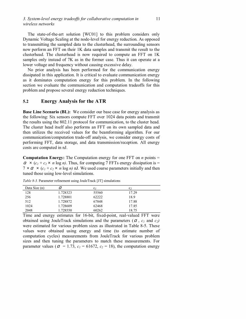
Base Line Scenario (BL): We consider our base case for energy analysis as the following: Six sensors compute FFT over 1024 data points and transmit the results using the 802.11 protocol for communication, to the cluster head. The cluster head itself also performs an FFT on its own sampled data and then utilizes the received values for the beamforming algorithm. For our communication/computation trade-off analysis, we consider energy costs of performing FFT, data storage, and data transmission/reception. All energy costs are computed in nJ. Computation Energy: The Computation energy for one FFT on n points = α × (c1 + c2 × n log n). Thus, for computing 7 FFTs energy dissipation is = 7 × α × (c1 + c2 × n log n) nJ. We used coarse parameters initially and then tuned those using low-level simulations. Table 8-3. Parameter refinement using JouleTrack [JT] simulations

Data Size (n) α c1 c2 128 1.728323 55560 17.29 256 1.728801 62222 18.9 512 1.728872 67848 17.88 1024 1.728609 62468 17.85 2048 1.728550 60262 18.75

Time and energy estimates for 16-bit, fixed-point, real-valued FFT were obtained using JouleTrack simulations and the parameters (α , c1 and c2) were estimated for various problem sizes as illustrated in Table 8-5. These values were obtained using energy and time (to estimate number of computation cycles) measurements from JouleTrack for various problem sizes and then tuning the parameters to match these measurements. For parameter values (α = 1.73, c1 = 61672, c2 = 18), the computation energy

12 Chapter 8 can be estimated as 7 × 1.73 × (61672 + 18 × n log n) = (0.75 x 106 + 218 n log n) nJ. Storage Energy: Consider 1 memory bank of size 4 MB to be sufficiently large to store data and program. Note the total data stored as a node is only 2n bytes and 14n at the cluster head. For n ≤ 1024 this is much smaller to 4 MB. The memory remains active for the entire time (1 sec to process one set of data). Assuming β = 90, storage energy is given by 360 nJ. This is negligible compared with the computation energy. Communication Energy: We assume 16-bit precision. Each node transmits n samples = 2n data bytes to the cluster head. In all there are 6 transmissions and receptions of data. The total communication energy is given by γ × 6 × 2 × 2n. For 802.11 we assume r = 31% (see Section 5.3). Thus total energy dissipation for communication between nodes is given by 77 × γ × n. For ≅γ 1000, energy dissipation is given by 77000n nJ. From our analysis, it is evident that the communication energy costs are much higher than computation energy costs. Thus, we focus upon reduction of communication energy at the expense of increased computation.

5.3 System-level Energy Tradeoffs

In this section we analyze several communication versus computation energy tradeoffs and apply them to the ATR application for obtaining overall energy reduction in the system.

Data Compression (DC): The communication energy can be decreased by reducing the amount of data that is transmitted to the clusterhead. For example data can be compressed or redundant data can be filtered out. We considered the LZW algorithm for our analysis. We generated random samples of data and compressed them using LZW. Data files with data samples ranging from 200 to 1800 were analyzed. On the average data compression reduced the resultant data to half its original number of bytes. The computation overheads were proportional to the data size being compressed. Figure 8-4 shows the overall energy reduction achieved as a function of the number of data samples to be transmitted. (Note that due to random generation of data the bytes transmitted are not always linearly proportional to the number of samples. Thus we see a glitch in the curve).


13

Figure 8-4. Energy analysis using data compression

We observed that for 1024 bytes of data with compression by a factor of two, we could reduce overall energy from 18.878 mJ to 14 mJ. However, a more effective technique was application specific data filtering. It was observed that the transmitted data represented frequency components of the acoustic data from 0-1024 Hz. Only the frequency range between 20-250 Hz is useful and needs to be transmitted. Remaining frequencies are not useful and can be filtered out. After computing the FFT, only the values corresponding to the useful frequency range were transmitted. Thus, the data to be transmitted was reduced to one fourth with negligible computation overheads.

Compression was applied after filtering the data. The resultant data was compressed by a factor of 0.3 with computation overheads of only 0.851 mJ. The data to be transmitted was reduced by one-sixth and overall energy dissipation was reduced to 3.934 mJ.

We applied a standard compression algorithm to reduce communication energy. Other coding and compression techniques must be evaluated for their computation overheads and the amount of compression achieved. C. Tang et al. [TR+02] are investigating application specific coding that exploits spatial and temporal correlation between successive data frames. Forward Error Correction (FEC): This technique involves large computation overheads for coding and decoding data. However, it permits transmission of data at a much lower signal power. For our analysis, we used convolutional coding and Viterbi decoding [TO]. We analyzed the energy tradeoffs for various values of parameter K, which represents the constraint

14 Chapter 8 length for the algorithm. The computational complexity of the decoding algorithm grows exponentially with K. The energy per symbol to noise density ratio for various bit error rates reduces with increasing K for an environment with a given BER as illustrated in Figure 8-5.

Figure 8-5. Rate 1/2 convolutional coding with Viterbi decoding on an AWGN channel with various convolutional code constraint lengths [TO]

We observed maximum overall energy reduction by choosing K = 3. The results are illustrated in Figure 8-6. The first bar represents the overall system energy for communicating 2048 bytes of data without using FEC. FEC with K = 3 reduces energy per symbol to noise density ratio by 3.5 dB (see Figure 8-5). Thus transmission power can be decreased by a factor of 3 resulting in lower communication energy as shown by the second bar in Figure 8-6. The third bar illustrates the energy overheads for computing FEC with K = 3. Lastly, the impact of using this technique on the overall energy (communication +computation overheads) is shown. Energy reduction by 50% can be achieved. Several other advanced codes [AH] promise energy per bit to noise ratio reduction up to 10 dB implying that the transmission power can be reduced by 10. However, it is important to examine them for the computation overheads involved.


15

Figure 8-6. Energy tradeoffs for FEC

Scheduling Transmissions (ST): The 6 surrounding nodes transmit data to the cluster head. Since, they begin transmitting at the same time (after computing FFT) in each period, a large number of collisions take place. Simulations using the 802.11 back off algorithm showed that on average over a million iterations, 19 time slots were required to transmit the data. Note we assume that a sensor sends all its data in a single time slot. The number of timeslots required can be reduced to 6 if TDMA scheduling is used for data transmission. The cluster head initiates the round of communication by sending a beacon signal. After hearing the beacon signal, each node knows exactly when to turn on the radio to transmit data to the cluster head. When one node transmits, the others are switched off. This reduces communication energy by 69% over the baseline scenario. The overheads for this scheme are in terms of time synchronization between nodes. However, in a 7-node cluster these are negligible. In larger settings these could become significantly high.

6. INTERPRETIVE SIMULATION RESULTS

In the previous section, we discussed several energy tradeoffs and their effect on the overall energy dissipation in the system. We used interpretive simulation results to obtain energy estimates. The computation costs were obtained using the JouleTrack simulator. The communication costs were estimated as a function of the data size received or transmitted, and the energy cost per byte for transmission and reception.

16 Chapter 8

In the first scenario the parameters (γ ,α ) were taken as (1000, 2) as illustrated in Table 8-4. Thus the communication to computation ratio (γ /α ) was assumed to be 500. The total computation costs for performing FFT, LOB and Beam forming were estimated as 3.28 mJ through simulations using Joule Track.

We assumed 2048 bytes to be sent from each periphery sensor to the clusterhead in the baseline (BL) case. The channel throughput using 802.11 protocol was assumed to be 31%. Based on these assumptions, the communication energy was estimated as 94.12 mJ resulting in an overall energy dissipation of 97.4 mJ.

Data Compression (DC) reduced the number of transmission bytes to one-fifth reducing communication energy to 15.68 mJ at an increased computation overhead of 9 mJ. Thus, the overall energy was reduced to 15.68 +10.2 + 3.28 = 29.16 mJ. Forward error Correction (FEC) permitted transmission power reduction by a factor of 3. The computation overheads involved were (5.337 × 6) mJ using Convolutional coding and Viterbi decoding with constraint length of 3. Scheduling Transmissions (ST) between the nodes, collisions were avoided and channel throughput was improved by 69%. Since the number of participating nodes is small and they are placed close to each other, synchronization overheads were considered to be negligible.

Figure 8-7. Energy Dissipation in the System with γ /α = 500

Lastly, the impact of applying all these simultaneously (ALL) was evaluated. The transmission power was reduced to one third, the data transmitted was reduced to one-fifth and no packet loss due to collisions was assumed. Note that the computation heads for the ALL case are smaller than


17

the sum of individual DC, FEC and ST cases. Data compression is used to reduce the data set to be transmitted. Thus, FEC is applied on a smaller data set resulting in smaller computation overheads. The overall system energy was reduced to 15.42 mJ. Thus an overall energy reduction by 80% was achieved as illustrated in Figure 8-7. Low power architectures are advancing rapidly. The above results are relevant in the current scenario. However, some of these techniques will not be beneficial in future when the energy metrics for the implementation platform change. We believe the ratio 500 that we used for our analysis will decrease in future with advancements in the technology. Figure 8-8 illustrates an energy prediction using a "futuristic scenario", where the ratio γ /α is reduced to 300. This is achieved by keeping α fixed and reducingγ .

Figure 8-8. Energy Dissipation in the System with γ /α = 300

The overall energy is reduced for all the scenarios including the baseline scenario. However, most of the techniques discussed are relatively less effective because computation overheads become significant. Techniques such as scheduled transmissions are not affected by this ratio since they had negligible computation overheads. In the new scenario, the communication energy for the application is reduced drastically, but the computation overheads are high. Thus, only overall energy reduction by 67% is achieved.

18 Chapter 8 7. Discussion

This paper is based on a �coarse� performance model that is utilized to obtain rapid estimates for overall energy dissipation in a small-sized wireless networks consisting of nodes performing collaborative computation. The model parameters for estimating energy costs for various operations were estimated. Based on the state-of-the-art, we assumed a ratio of 500 for the energy consumed to transmit a byte of data to that required for performing one cycle of computation.

Using this model, potential energy reduction for the ATR application was discussed. It was demonstrated that there is a nontrivial interplay between the various parameters in reducing overall system energy. For example, sophisticated compression techniques reduced the communication energy but at the expense of the node computation energy. Similarly, the storage overheads must be considered. Thus, this paper presents a vertically integrated approach that considers various knobs and energy optimization techniques in an integrated manner.

This paper highlights the benefits of using sophisticated coding [TR02+] and compression techniques for energy reduction. We will further explore algorithms that reduce data communication and permit more efficient error correction and evaluate them for the computation overheads. These would permit low power transmissions and improved performance even under extreme environmental conditions. The impact of communication/ computation energy efficiency ratio γ /α in system level energy optimization was also demonstrated. As this ratio reduces, performing communication in close neighbors as in the ATR application becomes less expensive. As a result of this, several node-level optimizations become relevant and their impact must be evaluated from the overall energy reduction perspective.

We also discussed integration of our model into the MILAN framework in Section 4. This permits construction of a system-level tool that can be utilized for obtaining rapid and yet accurate system energy estimations for various mappings and parameter settings. The high level model permits rapid design space exploration, while the hierarchical simulations improve accuracy of results by through refinement of model parameters using low-level simulations.

8. Acknowledgments

We would like to thank the participants of the PACMAN [TP] and MILAN [TM] projects for their valuable help and suggestions.


19

REFERENCES

[AH] Advanced Hardware Architectures. http://www.aha.com [AI] Yi-Qun Li, �An innovative passive solid-state magnetic sensor�, Sensors Magazine, Vol. 17, No. 10, October 2000. http://www.sensorsmag.com/articles/1000/52/main.shtml [BM99] L. Benini and G. D. Micheli, �System-Level Power Optimization: Techniques and Tools,� International Symposium on Low-Power Electronics and Design (ISLPED), August 1999. [BV02] A. Bakshi, and V. K. Prasanna, �Power-aware embedded system design using the MILAN framework,� IEEE Workshop on Integrated Management of Power Aware Communications, Computing and Networking (IMPACCT), May 2002. [DI] DARPA ITO, Power Aware Computing/Communication Program. http://www.darpa.mil/ito/research/pacc/index.html [EB02+] J.P. Ebert, B. Burns, and A. Wolisz, �A trace-based approach for determining the energy consumption of a WLAN network interface,� European Wireless, February 2002. [FN01] L. M. Feeney and M. Nilsson, �Investigating the energy consumption of a wireless network interface in an ad hoc networking environment,� IEEE International Conference on Computer Communication (INFOCOM), April 2001. [GK99] F. Gruian and K. Kuchcinski, �Low-energy directed architecture selection and task scheduling,� Euromicro Conference, September 1999. [JT] JouleTrack: A Web Based Software Energy Profiling Tool. http://dry-martini.mit.edu/JouleTrack/arm/ [KC01+] D. Kang, S. Crago, and J. Suh, �Power-aware design synthesis techniques for distributed real-time systems,� Workshop on Languages, Compilers, and Tools for Embedded Systems (LCTES), June 2001. [LR00+] M. Lajolo, A. Raghunathan, and S. Dey, �Efficient power co-estimation for system-on-chip design,� IEEE Design and Test Europe (DATE), March 2000. [LW] Lucent WaveLAN (ORINOCO). http://www.wavelan.com [MP02+] S. Mohanty, V. K. Prasanna, S. Neema, and J. Davis, �Rapid design space exploration of heterogeneous embedded systems using symbolic search and multi-granular simulation,� Workshop on Languages, Compilers, and Tools for Embedded Systems (LCTES), June 2002. [PB00+] T. Pering, T. Burd, and R. Broderson, �Dynamic voltage scaling and the design of a low-power microprocessor system,� International Symposium on Computer Architecture (ISCA), June 1998.

20 Chapter 8 [PR01+] D. Panigrahi, A. Raghunathan, G. Lakshminarayana, and S. Dey, �Energy modelling for wireless internet access,� IEEE International Conference on Third Generation Wireless and Beyond, May 2001. [SM] SA-1100 Models, The UAMPS Project. http://www.mtl.mit.edu/research/icsystems/uamps. [SR98] S. Singh and C. S. Raghavendra, �PAMAS: Power aware multi-access protocol with signalling for ad hoc networks,� ACM Computer Communications Review, Vol. 28, No. 3, pp. 5-26, July 1998. [TR02+] C. Tang, C. S. Raghavendra, and V. K. Prasanna, �An energy efficient distributed source coding scheme in wireless sensor networks,� Manuscript, Department of Electrical Engineering, USC, April 2002. [TM] The MILAN project. http://milan.usc.edu. [TO] Tutorial on convolutional coding with viterbi decoding, http://home.netcom.com/~chip.f/viterbi/simrslts.html [TP] The PACMAN project. http://pacman.usc.edu. [UA] US Army Research Laboratory. http://www.arl.mil. [WC01] A. Wang and A. Chandrakasan, �Energy efficient system partitioning for distributed wireless sensor networks,� IEEE International Conference on Acoustics, Speech, and Signal Processing (ICASSP), May 2001. [WE93] M. Weiser, �Some computer science issues in ubiquitous computing,� Communications of ACM, Vol. 36, No. 7, pp 75 � 84, July 1993. [YV00+] W.Ye, N.Vijaykrishnan, M.Kandemir, and M.J.Irwin, �The design and use of SimplePower: A cycle-accurate energy estimation tool,� IEEE/ACM Design Automation Conference (DAC), June 2000.

system-level energy tradeoffs for ...halcyon.usc.edu/~pk/prasannawebsite/papers/singhimpacct.pdf3....

Documents