system identification toolbox™ 7 user’s guide -...
TRANSCRIPT

System Identification Toolbox™ 7User’s Guide
Lennart Ljung
How to Contact The MathWorks
www.mathworks.com Webcomp.soft-sys.matlab Newsgroupwww.mathworks.com/contact_TS.html Technical [email protected] Product enhancement [email protected] Bug [email protected] Documentation error [email protected] Order status, license renewals, [email protected] Sales, pricing, and general information
508-647-7000 (Phone)
508-647-7001 (Fax)
The MathWorks, Inc.3 Apple Hill DriveNatick, MA 01760-2098For contact information about worldwide offices, see the MathWorks Web site.System Identification Toolbox™ User’s Guide© COPYRIGHT 1988–2008 by The MathWorks, Inc.The software described in this document is furnished under a license agreement. The software may be usedor copied only under the terms of the license agreement. No part of this manual may be photocopied orreproduced in any form without prior written consent from The MathWorks, Inc.FEDERAL ACQUISITION: This provision applies to all acquisitions of the Program and Documentationby, for, or through the federal government of the United States. By accepting delivery of the Programor Documentation, the government hereby agrees that this software or documentation qualifies ascommercial computer software or commercial computer software documentation as such terms are usedor defined in FAR 12.212, DFARS Part 227.72, and DFARS 252.227-7014. Accordingly, the terms andconditions of this Agreement and only those rights specified in this Agreement, shall pertain to and governthe use, modification, reproduction, release, performance, display, and disclosure of the Program andDocumentation by the federal government (or other entity acquiring for or through the federal government)and shall supersede any conflicting contractual terms or conditions. If this License fails to meet thegovernment’s needs or is inconsistent in any respect with federal procurement law, the government agreesto return the Program and Documentation, unused, to The MathWorks, Inc.
Trademarks
MATLAB and Simulink are registered trademarks of The MathWorks, Inc. Seewww.mathworks.com/trademarks for a list of additional trademarks. Other product or brandnames may be trademarks or registered trademarks of their respective holders.Patents
The MathWorks products are protected by one or more U.S. patents. Please seewww.mathworks.com/patents for more information.

Revision HistoryApril 1988 First printingJuly 1991 Second printingMay 1995 Third printingNovember 2000 Fourth printing Revised for Version 5.0 (Release 12)April 2001 Fifth printingJuly 2002 Online only Revised for Version 5.0.2 (Release 13)June 2004 Sixth printing Revised for Version 6.0.1 (Release 14)March 2005 Online only Revised for Version 6.1.1 (Release 14SP2)September 2005 Seventh printing Revised for Version 6.1.2 (Release 14SP3)March 2006 Online only Revised for Version 6.1.3 (Release 2006a)September 2006 Online only Revised for Version 6.2 (Release 2006b)March 2007 Online only Revised for Version 7.0 (Release 2007a)September 2007 Online only Revised for Version 7.1 (Release 2007b)March 2008 Online only Revised for Version 7.2 (Release 2008a)October 2008 Online only Revised for Version 7.2.1 (Release 2008b)


About the Developers
About the DevelopersSystem Identification Toolbox™ software is developed in association with thefollowing leading researchers in the system identification field:
Lennart Ljung. Professor Lennart Ljung is with the Department ofElectrical Engineering at Linköping University in Sweden. He is a recognizedleader in system identification and has published numerous papers and booksin this area.
Qinghua Zhang. Dr. Qinghua Zhang is a researcher at Institut Nationalde Recherche en Informatique et en Automatique (INRIA) and at Institut deRecherche en Informatique et Systèmes Aléatoires (IRISA), both in Rennes,France. He conducts research in the areas of nonlinear system identification,fault diagnosis, and signal processing with applications in the fields of energy,automotive, and biomedical systems.
Peter Lindskog. Dr. Peter Lindskog is employed by NIRA DynamicsAB, Sweden. He conducts research in the areas of system identification,signal processing, and automatic control with a focus on vehicle industryapplications.
Anatoli Juditsky. Professor Anatoli Juditsky is with the Laboratoire JeanKuntzmann at the Université Joseph Fourier, Grenoble, France. He conductsresearch in the areas of nonparametric statistics, system identification, andstochastic optimization.

About the Developers

Contents
Data Processing
1Ways to Process Data for System Identification . . . . . . . 1-2
Importing Data into the MATLAB Workspace . . . . . . . . 1-5Types of Data You Can Model . . . . . . . . . . . . . . . . . . . . . . . 1-5Support for Data with Uniform and Nonuniform SamplingIntervals . . . . . . . . . . . . . . . . . . . . . . . . . . . . . . . . . . . . . . 1-6
Importing Time-Domain Data into MATLAB . . . . . . . . . . . 1-6Importing Time-Series Data into MATLAB . . . . . . . . . . . . 1-7Importing Frequency-Domain Data into MATLAB . . . . . . 1-8Importing Frequency-Response Data into MATLAB . . . . . 1-10
Representing Data in the GUI . . . . . . . . . . . . . . . . . . . . . . 1-13Types of Data You Can Import into the GUI . . . . . . . . . . . . 1-13Importing Time-Domain Data into the GUI . . . . . . . . . . . . 1-15Importing Frequency-Domain Data into the GUI . . . . . . . . 1-18Importing Frequency-Response Data into the GUI . . . . . . 1-21Importing Data Objects into the GUI . . . . . . . . . . . . . . . . . 1-25Specifying the Data Sampling Interval . . . . . . . . . . . . . . . . 1-28Specifying Estimation and Validation Data . . . . . . . . . . . . 1-29Preprocessing Data Using Quick Start . . . . . . . . . . . . . . . . 1-30Creating Data Sets from a Subset of Signal Channels . . . . 1-31Creating Multiexperiment Data Sets in the GUI . . . . . . . . 1-33Viewing Data Properties . . . . . . . . . . . . . . . . . . . . . . . . . . . . 1-40Renaming Data and Changing Display Color . . . . . . . . . . . 1-41Distinguishing Data Types in the GUI . . . . . . . . . . . . . . . . 1-43Organizing Data Icons . . . . . . . . . . . . . . . . . . . . . . . . . . . . . 1-43Deleting Data Sets in the GUI . . . . . . . . . . . . . . . . . . . . . . . 1-44Exporting Data from the GUI to the MATLABWorkspace . . . . . . . . . . . . . . . . . . . . . . . . . . . . . . . . . . . . . 1-45
Representing Time- and Frequency-Domain Data Usingiddata Objects . . . . . . . . . . . . . . . . . . . . . . . . . . . . . . . . . . . 1-47iddata Constructor . . . . . . . . . . . . . . . . . . . . . . . . . . . . . . . . 1-47iddata Properties . . . . . . . . . . . . . . . . . . . . . . . . . . . . . . . . . . 1-50
vii

Creating Multiexperiment Data at the Command Line . . . 1-53Subreferencing iddata Objects . . . . . . . . . . . . . . . . . . . . . . . 1-55Modifying Time and Frequency Vectors . . . . . . . . . . . . . . . 1-59Naming, Adding, and Removing Data Channels . . . . . . . . . 1-63Concatenating iddata Objects . . . . . . . . . . . . . . . . . . . . . . . 1-65
Representing Frequency-Response Data Using idfrdObjects . . . . . . . . . . . . . . . . . . . . . . . . . . . . . . . . . . . . . . . . . 1-67idfrd Constructor . . . . . . . . . . . . . . . . . . . . . . . . . . . . . . . . . . 1-67idfrd Properties . . . . . . . . . . . . . . . . . . . . . . . . . . . . . . . . . . . 1-68Subreferencing idfrd Objects . . . . . . . . . . . . . . . . . . . . . . . . 1-70Concatenating idfrd Objects . . . . . . . . . . . . . . . . . . . . . . . . . 1-71See Also . . . . . . . . . . . . . . . . . . . . . . . . . . . . . . . . . . . . . . . . . 1-74
Analyzing Data Quality Using Plots . . . . . . . . . . . . . . . . . 1-75Supported Data Plots . . . . . . . . . . . . . . . . . . . . . . . . . . . . . . 1-75Plotting Data in the System Identification Tool GUI . . . . . 1-75Plotting Data at the Command Line . . . . . . . . . . . . . . . . . . 1-81
Getting Advice About Your Data . . . . . . . . . . . . . . . . . . . . 1-84
Selecting Subsets of Data . . . . . . . . . . . . . . . . . . . . . . . . . . . 1-86Why Select Subsets of Data? . . . . . . . . . . . . . . . . . . . . . . . . 1-86Selecting Data Using the GUI . . . . . . . . . . . . . . . . . . . . . . . 1-87Selecting Data at the Command Line . . . . . . . . . . . . . . . . . 1-89
Handling Missing Data and Outliers . . . . . . . . . . . . . . . . . 1-90Handling Missing Data . . . . . . . . . . . . . . . . . . . . . . . . . . . . . 1-90Handling Outliers . . . . . . . . . . . . . . . . . . . . . . . . . . . . . . . . . 1-91Example – Extracting and Modeling Specific DataSegments . . . . . . . . . . . . . . . . . . . . . . . . . . . . . . . . . . . . . . 1-92
See Also . . . . . . . . . . . . . . . . . . . . . . . . . . . . . . . . . . . . . . . . . 1-93
Subtracting Trends from Signals (Detrending) . . . . . . . 1-94What Is Detrending? . . . . . . . . . . . . . . . . . . . . . . . . . . . . . . . 1-94When to Detrend Data . . . . . . . . . . . . . . . . . . . . . . . . . . . . . 1-94When Not to Detrend Data . . . . . . . . . . . . . . . . . . . . . . . . . . 1-95GUI and Command-Line Alternatives for DetrendingData . . . . . . . . . . . . . . . . . . . . . . . . . . . . . . . . . . . . . . . . . . 1-96
How to Detrend Data Using the GUI . . . . . . . . . . . . . . . . . . 1-96How to Detrend Data at the Command Line . . . . . . . . . . . . 1-97
viii Contents

How to Add Detrended Values to the Model Output . . . . . 1-98
Resampling Data . . . . . . . . . . . . . . . . . . . . . . . . . . . . . . . . . . 1-100What Is Resampling? . . . . . . . . . . . . . . . . . . . . . . . . . . . . . . 1-100Resampling Data Using the GUI . . . . . . . . . . . . . . . . . . . . . 1-101Resampling Data at the Command Line . . . . . . . . . . . . . . . 1-101Resampling Data Without Aliasing Effects . . . . . . . . . . . . . 1-103See Also . . . . . . . . . . . . . . . . . . . . . . . . . . . . . . . . . . . . . . . . . 1-106
Filtering Data . . . . . . . . . . . . . . . . . . . . . . . . . . . . . . . . . . . . . 1-107Supported Filters . . . . . . . . . . . . . . . . . . . . . . . . . . . . . . . . . 1-107Choosing to Prefilter Your Data . . . . . . . . . . . . . . . . . . . . . . 1-107How to Filter Data Using the GUI . . . . . . . . . . . . . . . . . . . . 1-108How to Filter Data at the Command Line . . . . . . . . . . . . . . 1-111See Also . . . . . . . . . . . . . . . . . . . . . . . . . . . . . . . . . . . . . . . . . 1-114
Generating Data Using Simulation . . . . . . . . . . . . . . . . . . 1-115Commands for Generating and Simulating Data . . . . . . . . 1-115Example – Creating Data with Periodic Inputs . . . . . . . . . 1-116Example – Generating Data Using Simulation . . . . . . . . . . 1-117Simulating Data Using Other MathWorks Products . . . . . 1-118
Transforming Between Time- and Frequency-DomainData . . . . . . . . . . . . . . . . . . . . . . . . . . . . . . . . . . . . . . . . . . . . 1-119Transforming Data Domain in the GUI . . . . . . . . . . . . . . . . 1-119Transforming Data Domain at the Command Line . . . . . . 1-126
Manipulating Complex-Valued Data . . . . . . . . . . . . . . . . . 1-131Supported Operations for Complex Data . . . . . . . . . . . . . . . 1-131Processing Complex iddata Signals at the CommandLine . . . . . . . . . . . . . . . . . . . . . . . . . . . . . . . . . . . . . . . . . . 1-131
Choosing Your System Identification Strategy
2Recommended Model Estimation Sequence . . . . . . . . . . 2-2
ix
Supported Models for Time- and Frequency-DomainData . . . . . . . . . . . . . . . . . . . . . . . . . . . . . . . . . . . . . . . . . . . . 2-4Supported Models for Time-Domain Data . . . . . . . . . . . . . . 2-4Supported Models for Frequency-Domain Data . . . . . . . . . 2-5
Supported Continuous-Time and Discrete-TimeModels . . . . . . . . . . . . . . . . . . . . . . . . . . . . . . . . . . . . . . . . . 2-7
Commands for Model Estimation . . . . . . . . . . . . . . . . . . . . 2-9
Creating Model Structures at the Command Line . . . . . 2-11About System Identification Toolbox Model Objects . . . . . . 2-11When to Construct a Model Structure Independently ofEstimation . . . . . . . . . . . . . . . . . . . . . . . . . . . . . . . . . . . . . 2-12
Commands for Constructing Model Structures . . . . . . . . . . 2-13Model Properties . . . . . . . . . . . . . . . . . . . . . . . . . . . . . . . . . . 2-14See Also . . . . . . . . . . . . . . . . . . . . . . . . . . . . . . . . . . . . . . . . . 2-20
Modeling Multiple-Output Systems . . . . . . . . . . . . . . . . . . 2-21About Modeling Multiple-Output Systems . . . . . . . . . . . . . 2-21Modeling Multiple Outputs Directly . . . . . . . . . . . . . . . . . . 2-22Modeling Multiple Outputs as a Combination ofSingle-Output Models . . . . . . . . . . . . . . . . . . . . . . . . . . . . 2-22
Improving Multiple-Output Estimation Results byWeighing Outputs During Estimation . . . . . . . . . . . . . . 2-23
Linear Model Identification3
Identifying Frequency-Response Models . . . . . . . . . . . . . 3-2What Is a Frequency-Response Model? . . . . . . . . . . . . . . . . 3-2Data Supported by Frequency-Response Models . . . . . . . . 3-3How to Estimate Frequency-Response Models in theGUI . . . . . . . . . . . . . . . . . . . . . . . . . . . . . . . . . . . . . . . . . . 3-3
How to Estimate Frequency-Response Models at theCommand Line . . . . . . . . . . . . . . . . . . . . . . . . . . . . . . . . . 3-5
Options for Computing Spectral Models . . . . . . . . . . . . . . . 3-5Options for Frequency Resolution . . . . . . . . . . . . . . . . . . . . 3-6Spectral Analysis Algorithm . . . . . . . . . . . . . . . . . . . . . . . . . 3-8
x Contents
Understanding Spectrum Normalization . . . . . . . . . . . . . . 3-11
Identifying Impulse-Response Models . . . . . . . . . . . . . . . 3-14What Is Time-Domain Correlation Analysis? . . . . . . . . . . . 3-14Data Supported by Correlation Analysis . . . . . . . . . . . . . . . 3-15How to Estimate Correlation Models Using the GUI . . . . . 3-15How to Estimate Correlation Models at the CommandLine . . . . . . . . . . . . . . . . . . . . . . . . . . . . . . . . . . . . . . . . . . 3-16
How to Compute Response Values . . . . . . . . . . . . . . . . . . . . 3-18How to Identify Delay Using Transient-Response Plots . . . 3-18Algorithm for Correlation Analysis . . . . . . . . . . . . . . . . . . . 3-20
Identifying Low-Order Transfer Functions (ProcessModels) . . . . . . . . . . . . . . . . . . . . . . . . . . . . . . . . . . . . . . . . . 3-22What Is a Process Model? . . . . . . . . . . . . . . . . . . . . . . . . . . . 3-22Data Supported by a Process Model . . . . . . . . . . . . . . . . . . . 3-23How to Estimate Process Models Using the GUI . . . . . . . . 3-23Estimating Process Models at the Command Line . . . . . . . 3-29Options for Specifying the Process-Model Structure . . . . . 3-35Options for Multiple-Input Models . . . . . . . . . . . . . . . . . . . 3-36Options for the Disturbance Model Structure . . . . . . . . . . . 3-37Options for Frequency-Weighing Focus . . . . . . . . . . . . . . . . 3-38Options for Initial States . . . . . . . . . . . . . . . . . . . . . . . . . . . 3-39
Identifying Input-Output Polynomial Models . . . . . . . . 3-41What Are Black-Box Polynomial Models? . . . . . . . . . . . . . . 3-41Data Supported by Polynomial Models . . . . . . . . . . . . . . . . 3-48Preliminary Step – Estimating Model Orders and InputDelays . . . . . . . . . . . . . . . . . . . . . . . . . . . . . . . . . . . . . . . . 3-49
How to Estimate Polynomial Models in the GUI . . . . . . . . 3-57How to Estimate Polynomial Models at the CommandLine . . . . . . . . . . . . . . . . . . . . . . . . . . . . . . . . . . . . . . . . . . 3-60
Options for Multiple-Input and Multiple-Output ARXOrders . . . . . . . . . . . . . . . . . . . . . . . . . . . . . . . . . . . . . . . . 3-64
Option for Frequency-Weighing Focus . . . . . . . . . . . . . . . . . 3-65Options for Initial States . . . . . . . . . . . . . . . . . . . . . . . . . . . 3-66Algorithms for Estimating Polynomial Models . . . . . . . . . . 3-66Example – Estimating Models Using armax . . . . . . . . . . . . 3-67
Identifying State-Space Models . . . . . . . . . . . . . . . . . . . . . 3-73What Are State-Space Models? . . . . . . . . . . . . . . . . . . . . . . 3-73Data Supported by State-Space Models . . . . . . . . . . . . . . . . 3-77
xi

Supported State-Space Parameterizations . . . . . . . . . . . . . 3-78Preliminary Step – Estimating State-Space ModelOrders . . . . . . . . . . . . . . . . . . . . . . . . . . . . . . . . . . . . . . . . 3-79
How to Estimate State-Space Models in the GUI . . . . . . . . 3-84How to Estimate State-Space Models at the CommandLine . . . . . . . . . . . . . . . . . . . . . . . . . . . . . . . . . . . . . . . . . . 3-87
How to Estimate Free-Parameterization State-SpaceModels . . . . . . . . . . . . . . . . . . . . . . . . . . . . . . . . . . . . . . . . 3-90
How to Estimate State-Space Models with CanonicalParameterization . . . . . . . . . . . . . . . . . . . . . . . . . . . . . . . 3-91
How to Estimate State-Space Models with StructuredParameterization . . . . . . . . . . . . . . . . . . . . . . . . . . . . . . . 3-93
How to Estimate the State-Space Equivalent of ARMAXand OE Models . . . . . . . . . . . . . . . . . . . . . . . . . . . . . . . . . 3-100
Options for Frequency-Weighing Focus . . . . . . . . . . . . . . . . 3-100Options for Initial States . . . . . . . . . . . . . . . . . . . . . . . . . . . 3-101Algorithms for Estimating State-Space Models . . . . . . . . . 3-101
Refining Linear Parametric Models . . . . . . . . . . . . . . . . . 3-103When to Refine Models . . . . . . . . . . . . . . . . . . . . . . . . . . . . . 3-103What You Specify to Refine a Model . . . . . . . . . . . . . . . . . . 3-103How to Refine Linear Parametric Models in the GUI . . . . . 3-104How to Refine Linear Parametric Models at the CommandLine . . . . . . . . . . . . . . . . . . . . . . . . . . . . . . . . . . . . . . . . . . 3-105
Extracting Parameter Values from Linear Models . . . . 3-108
Extracting Dynamic Model and Noise ModelSeparately . . . . . . . . . . . . . . . . . . . . . . . . . . . . . . . . . . . . . . 3-110
Transforming Between Discrete-Time andContinuous-Time Representations . . . . . . . . . . . . . . . . 3-112Why Transform Between Continuous and DiscreteTime? . . . . . . . . . . . . . . . . . . . . . . . . . . . . . . . . . . . . . . . . . 3-112
Using the c2d, d2c, and d2d Commands . . . . . . . . . . . . . . . 3-112Specifying Intersample Behavior . . . . . . . . . . . . . . . . . . . . . 3-114How d2c Handles Input Delays . . . . . . . . . . . . . . . . . . . . . . 3-114Effects on the Noise Model . . . . . . . . . . . . . . . . . . . . . . . . . . 3-115
Transforming Between Linear ModelRepresentations . . . . . . . . . . . . . . . . . . . . . . . . . . . . . . . . . 3-117
xii Contents

Subreferencing Model Objects . . . . . . . . . . . . . . . . . . . . . . 3-119What Is Subreferencing? . . . . . . . . . . . . . . . . . . . . . . . . . . . . 3-119Limitation on Supported Models . . . . . . . . . . . . . . . . . . . . . 3-119Subreferencing Specific Measured Channels . . . . . . . . . . . 3-119Subreferencing Measured and Noise Models . . . . . . . . . . . 3-120Treating Noise Channels as Measured Inputs . . . . . . . . . . 3-122
Concatenating Model Objects . . . . . . . . . . . . . . . . . . . . . . . 3-124About Concatenating Models . . . . . . . . . . . . . . . . . . . . . . . . 3-124Limitation on Supported Models . . . . . . . . . . . . . . . . . . . . . 3-124Horizontal Concatenation of Model Objects . . . . . . . . . . . . 3-125Vertical Concatenation of Model Objects . . . . . . . . . . . . . . . 3-125Concatenating Noise Spectral Data of idfrd Objects . . . . . . 3-126See Also . . . . . . . . . . . . . . . . . . . . . . . . . . . . . . . . . . . . . . . . . 3-127
Merging Model Objects . . . . . . . . . . . . . . . . . . . . . . . . . . . . . 3-128
Nonlinear Black-Box Model Identification4
Supported Data for Estimating Nonlinear Black-BoxModels . . . . . . . . . . . . . . . . . . . . . . . . . . . . . . . . . . . . . . . . . 4-2
Supported Nonlinear Black-Box Models . . . . . . . . . . . . . 4-3
Identifying Nonlinear ARX Models . . . . . . . . . . . . . . . . . . 4-4Supported Data for Nonlinear ARX Models . . . . . . . . . . . . 4-4Definition of the Nonlinear ARX Model . . . . . . . . . . . . . . . . 4-4Using Regressors . . . . . . . . . . . . . . . . . . . . . . . . . . . . . . . . . . 4-6Nonlinearity Estimators for Nonlinear ARX Models . . . . . 4-9How to Estimate Nonlinear ARX Models in the GUI . . . . . 4-10How to Estimate Nonlinear ARX Models at the CommandLine . . . . . . . . . . . . . . . . . . . . . . . . . . . . . . . . . . . . . . . . . . 4-11
Identifying Hammerstein-Wiener Models . . . . . . . . . . . . 4-15Supported Data for Estimating Hammerstein-WienerModels . . . . . . . . . . . . . . . . . . . . . . . . . . . . . . . . . . . . . . . . 4-15
Definition of the Hammerstein-Wiener Model . . . . . . . . . . 4-15
xiii

Nonlinearity Estimators for Hammerstein-WienerModels . . . . . . . . . . . . . . . . . . . . . . . . . . . . . . . . . . . . . . . . 4-17
How to Estimate Hammerstein-Wiener Models in theGUI . . . . . . . . . . . . . . . . . . . . . . . . . . . . . . . . . . . . . . . . . . 4-18
How to Estimate Hammerstein-Wiener Models at theCommand Line . . . . . . . . . . . . . . . . . . . . . . . . . . . . . . . . . 4-20
Supported Nonlinearity Estimators . . . . . . . . . . . . . . . . . 4-25Types of Nonlinearity Estimators . . . . . . . . . . . . . . . . . . . . 4-25Creating Custom Nonlinearities . . . . . . . . . . . . . . . . . . . . . 4-26
Refining Nonlinear Black-Box Models . . . . . . . . . . . . . . . 4-28How to Refine Nonlinear Black-Box Models in the GUI . . . 4-28How to Refine Nonlinear Black-Box Models at the CommandLine . . . . . . . . . . . . . . . . . . . . . . . . . . . . . . . . . . . . . . . . . . 4-29
Extracting Parameter Values from Nonlinear Black-BoxModels . . . . . . . . . . . . . . . . . . . . . . . . . . . . . . . . . . . . . . . . . 4-30Nonlinear ARX Parameter Values . . . . . . . . . . . . . . . . . . . . 4-30Hammerstein-Wiener Parameter values . . . . . . . . . . . . . . . 4-31
Next Steps After Estimating Nonlinear Black-BoxModels . . . . . . . . . . . . . . . . . . . . . . . . . . . . . . . . . . . . . . . . . 4-32
Computing Linear Approximations of NonlinearBlack-Box Models . . . . . . . . . . . . . . . . . . . . . . . . . . . . . . . 4-33Why Compute a Linearize Approximation of a NonlinearModel? . . . . . . . . . . . . . . . . . . . . . . . . . . . . . . . . . . . . . . . . 4-33
Choosing Your Linear Approximation Approach . . . . . . . . 4-33Linear Approximation of Nonlinear Black-Box Models for aGiven Input . . . . . . . . . . . . . . . . . . . . . . . . . . . . . . . . . . . . 4-34
Tangent Linearization of Nonlinear Black-Box Models . . . 4-35Computing Operating Points for Nonlinear Black-BoxModels . . . . . . . . . . . . . . . . . . . . . . . . . . . . . . . . . . . . . . . . 4-35
xiv Contents

ODE Parameter Estimation (Grey-BoxModeling)
5Supported Grey-Box Models . . . . . . . . . . . . . . . . . . . . . . . . 5-2
Data Supported by Grey-Box Models . . . . . . . . . . . . . . . . 5-3
Choosing idgrey or idnlgrey Model Object . . . . . . . . . . . 5-4
Estimating Linear Grey-Box Models . . . . . . . . . . . . . . . . . 5-6Specifying the Linear Grey-Box Model Structure . . . . . . . . 5-6Example – Representing a Grey-Box Model in an M-File . . 5-7Example – Estimating a Continuous-Time Grey-Box Modelfor Heat Diffusion . . . . . . . . . . . . . . . . . . . . . . . . . . . . . . . 5-9
Example – Estimating a Discrete-Time Grey-Box Modelwith Parameterized Disturbance . . . . . . . . . . . . . . . . . . . 5-12
Estimating Nonlinear Grey-Box Models . . . . . . . . . . . . . . 5-16Supported Nonlinear Grey-Box Models . . . . . . . . . . . . . . . . 5-16Nonlinear Grey-Box Demos and Examples . . . . . . . . . . . . . 5-16Specifying the Nonlinear Grey-Box Model Structure . . . . . 5-17Constructing the idnlgrey Object . . . . . . . . . . . . . . . . . . . . . 5-18Using pem to Estimate Nonlinear Grey-Box Models . . . . . 5-19Options for the Estimation Algorithm . . . . . . . . . . . . . . . . . 5-20
After Estimating Grey-Box Models . . . . . . . . . . . . . . . . . . 5-23
Time Series Model Identification6
What Are Time-Series Models? . . . . . . . . . . . . . . . . . . . . . . 6-2
Preparing Time-Series Data . . . . . . . . . . . . . . . . . . . . . . . . 6-3
Estimating Time-Series Power Spectra . . . . . . . . . . . . . . 6-4
xv

How to Estimate Time-Series Power Spectra Using theGUI . . . . . . . . . . . . . . . . . . . . . . . . . . . . . . . . . . . . . . . . . . 6-4
How to Estimate Time-Series Power Spectra at theCommand Line . . . . . . . . . . . . . . . . . . . . . . . . . . . . . . . . . 6-5
Estimating AR and ARMA Models . . . . . . . . . . . . . . . . . . . 6-7Definition of AR and ARMA Models . . . . . . . . . . . . . . . . . . . 6-7Estimating Polynomial Time-Series Models in the GUI . . . 6-7Estimating AR and ARMA Models at the CommandLine . . . . . . . . . . . . . . . . . . . . . . . . . . . . . . . . . . . . . . . . . . 6-10
Estimating State-Space Time-Series Models . . . . . . . . . . 6-12Definition of State-Space Time-Series Model . . . . . . . . . . . 6-12Estimating State-Space Models at the Command Line . . . 6-12
Example – Identifying Time-Series Models at theCommand Line . . . . . . . . . . . . . . . . . . . . . . . . . . . . . . . . . . 6-14
Estimating Nonlinear Models for Time-Series Data . . . 6-15
Recursive Techniques for Model Identification
7What Is Recursive Estimation? . . . . . . . . . . . . . . . . . . . . . . 7-2
Commands for Recursive Estimation . . . . . . . . . . . . . . . . 7-3
Algorithms for Recursive Estimation . . . . . . . . . . . . . . . . 7-6Types of Recursive Estimation Algorithms . . . . . . . . . . . . . 7-6General Form of Recursive Estimation Algorithm . . . . . . . 7-6Kalman Filter Algorithm . . . . . . . . . . . . . . . . . . . . . . . . . . . 7-8Forgetting Factor Algorithm . . . . . . . . . . . . . . . . . . . . . . . . 7-10Unnormalized and Normalized Gradient Algorithms . . . . . 7-11
Data Segmentation . . . . . . . . . . . . . . . . . . . . . . . . . . . . . . . . 7-14
xvi Contents
Model Analysis
8Overview of Model Validation and Plots . . . . . . . . . . . . . 8-2When to Validate Models . . . . . . . . . . . . . . . . . . . . . . . . . . . 8-2Ways to Validate Models . . . . . . . . . . . . . . . . . . . . . . . . . . . 8-2Data for Validating Models . . . . . . . . . . . . . . . . . . . . . . . . . 8-4Supported Model Plots . . . . . . . . . . . . . . . . . . . . . . . . . . . . . 8-4Plotting Models in the GUI . . . . . . . . . . . . . . . . . . . . . . . . . . 8-5Getting Advice About Models . . . . . . . . . . . . . . . . . . . . . . . . 8-7
Using Model Output Plots to Validate and CompareModels . . . . . . . . . . . . . . . . . . . . . . . . . . . . . . . . . . . . . . . . . 8-8Supported Model Types . . . . . . . . . . . . . . . . . . . . . . . . . . . . 8-8What Does a Model Output Plot Show? . . . . . . . . . . . . . . . . 8-8Choosing Simulated or Predicted Output . . . . . . . . . . . . . . 8-9How to Plot Model Output Using the GUI . . . . . . . . . . . . . . 8-11Displaying the Confidence Interval . . . . . . . . . . . . . . . . . . . 8-13How to Plot and Compare Model Output at the CommandLine . . . . . . . . . . . . . . . . . . . . . . . . . . . . . . . . . . . . . . . . . . 8-14
Using Residual Analysis Plots to Validate Models . . . . . 8-16What Is Residual Analysis? . . . . . . . . . . . . . . . . . . . . . . . . . 8-16Supported Model Types . . . . . . . . . . . . . . . . . . . . . . . . . . . . 8-17What Does the Residuals Plot Show? . . . . . . . . . . . . . . . . . 8-17Displaying the Confidence Interval . . . . . . . . . . . . . . . . . . . 8-18How to Plot Residuals Using the GUI . . . . . . . . . . . . . . . . . 8-19How to Plot Residuals at the Command Line . . . . . . . . . . . 8-21Example – Examining Model Residuals . . . . . . . . . . . . . . . 8-21
Using Impulse- and Step-Response Plots to ValidateModels . . . . . . . . . . . . . . . . . . . . . . . . . . . . . . . . . . . . . . . . . 8-24Supported Models . . . . . . . . . . . . . . . . . . . . . . . . . . . . . . . . . 8-24How Transient Response Helps to Validate Models . . . . . . 8-24What Does a Transient Response Plot Show? . . . . . . . . . . . 8-25How to Plot Impulse and Step Response Using the GUI . . 8-26Displaying the Confidence Interval . . . . . . . . . . . . . . . . . . . 8-29How to Plot Impulse and Step Response at the CommandLine . . . . . . . . . . . . . . . . . . . . . . . . . . . . . . . . . . . . . . . . . . 8-30
Using Frequency-Response Plots to Validate Models . . 8-32
xvii

What Is Frequency Response? . . . . . . . . . . . . . . . . . . . . . . . 8-32How Frequency Response Helps to Validate Models . . . . . 8-33What Does a Frequency-Response Plot Show? . . . . . . . . . . 8-34How to Plot Bode Plots Using the GUI . . . . . . . . . . . . . . . . 8-35How to Plot Bode and Nyquist Plots at the CommandLine . . . . . . . . . . . . . . . . . . . . . . . . . . . . . . . . . . . . . . . . . . 8-38
Creating Noise-Spectrum Plots . . . . . . . . . . . . . . . . . . . . . 8-40Supported Models . . . . . . . . . . . . . . . . . . . . . . . . . . . . . . . . . 8-40What Does a Noise Spectrum Plot Show? . . . . . . . . . . . . . . 8-40Displaying the Confidence Interval . . . . . . . . . . . . . . . . . . . 8-41How to Plot the Noise Spectrum Using the GUI . . . . . . . . . 8-42How to Plot the Noise Spectrum at the Command Line . . . 8-45
Using Pole-Zero Plots to Validate Models . . . . . . . . . . . . 8-47Supported Models . . . . . . . . . . . . . . . . . . . . . . . . . . . . . . . . . 8-47What Does a Pole-Zero Plot Show? . . . . . . . . . . . . . . . . . . . 8-47How to Plot Model Poles and Zeros Using the GUI . . . . . . 8-48How to Plot Poles and Zeros at the Command Line . . . . . . 8-50Reducing Model Order Using Pole-Zero Plots . . . . . . . . . . . 8-51
Using Nonlinear ARX Plots to Validate Models . . . . . . . 8-52About Nonlinear ARX Plots . . . . . . . . . . . . . . . . . . . . . . . . . 8-52How to Plot Nonlinear ARX Plots Using the GUI . . . . . . . . 8-52Configuring the Nonlinear ARX Plot . . . . . . . . . . . . . . . . . . 8-53Axis Limits, Legend, and 3-D Rotation . . . . . . . . . . . . . . . . 8-54How to Plot Nonlinear ARX Plots at the Command Line . . 8-55
Using Hammerstein-Wiener Plots to ValidateModels . . . . . . . . . . . . . . . . . . . . . . . . . . . . . . . . . . . . . . . . . 8-56About Hammerstein-Wiener Plots . . . . . . . . . . . . . . . . . . . . 8-56How to Create Hammerstein-Wiener Plots in the GUI . . . 8-56How to Plot Hammerstein-Wiener Plots at the CommandLine . . . . . . . . . . . . . . . . . . . . . . . . . . . . . . . . . . . . . . . . . . 8-58
Plotting Nonlinear Block Characteristics . . . . . . . . . . . . . . 8-58Plotting Linear Block Characteristics . . . . . . . . . . . . . . . . . 8-59
Using Akaike’s Criteria to Validate Models . . . . . . . . . . . 8-61Definition of FPE . . . . . . . . . . . . . . . . . . . . . . . . . . . . . . . . . . 8-61Computing FPE . . . . . . . . . . . . . . . . . . . . . . . . . . . . . . . . . . . 8-62Definition of AIC . . . . . . . . . . . . . . . . . . . . . . . . . . . . . . . . . . 8-62Computing AIC . . . . . . . . . . . . . . . . . . . . . . . . . . . . . . . . . . . 8-63
xviii Contents
Computing Model Uncertainty . . . . . . . . . . . . . . . . . . . . . . 8-64Why Analyze Model Uncertainty? . . . . . . . . . . . . . . . . . . . . 8-64What Is Model Covariance? . . . . . . . . . . . . . . . . . . . . . . . . . 8-64Viewing Model Uncertainty Information . . . . . . . . . . . . . . . 8-65
Troubleshooting Models . . . . . . . . . . . . . . . . . . . . . . . . . . . . 8-67About Troubleshooting Models . . . . . . . . . . . . . . . . . . . . . . . 8-67Model Order Is Too High or Too Low . . . . . . . . . . . . . . . . . . 8-67Nonlinearity Estimator Produces a Poor Fit . . . . . . . . . . . . 8-68Substantial Noise in the System . . . . . . . . . . . . . . . . . . . . . 8-69Unstable Models . . . . . . . . . . . . . . . . . . . . . . . . . . . . . . . . . . 8-69Missing Input Variables . . . . . . . . . . . . . . . . . . . . . . . . . . . . 8-70Complicated Nonlinearities . . . . . . . . . . . . . . . . . . . . . . . . . 8-71
Next Steps After Getting an Accurate Model . . . . . . . . . 8-72
Simulation and Prediction9
Simulating Versus Predicting Output . . . . . . . . . . . . . . . 9-2
Simulation and Prediction in the GUI . . . . . . . . . . . . . . . 9-4
Example – Simulating Model Output with Noise at theCommand Line . . . . . . . . . . . . . . . . . . . . . . . . . . . . . . . . . . 9-5
Example – Simulating a Continuous-Time State-SpaceModel at the Command Line . . . . . . . . . . . . . . . . . . . . . . 9-6
Predicting Model Output at the Command Line . . . . . . 9-7
Specifying Initial States . . . . . . . . . . . . . . . . . . . . . . . . . . . . 9-8When to Specify Initial States . . . . . . . . . . . . . . . . . . . . . . . 9-8Setting Initial States to Zero . . . . . . . . . . . . . . . . . . . . . . . . 9-8Setting Initial States to Equilibrium Values . . . . . . . . . . . . 9-9Estimating Initial States from the Data . . . . . . . . . . . . . . . 9-9
xix

Using Identified Models in Control Design
10UsingModels with Control System Toolbox Software . . 10-2How Control System Toolbox Software Works withIdentified Models . . . . . . . . . . . . . . . . . . . . . . . . . . . . . . . 10-2
Using balred to Reduce Model Order . . . . . . . . . . . . . . . . . . 10-3Compensator Design Using Control System ToolboxSoftware . . . . . . . . . . . . . . . . . . . . . . . . . . . . . . . . . . . . . . . 10-3
Converting Models to LTI Objects . . . . . . . . . . . . . . . . . . . . 10-4Viewing Model Response Using the LTI Viewer . . . . . . . . . 10-5Combining Model Objects . . . . . . . . . . . . . . . . . . . . . . . . . . . 10-6Example – Using System Identification Toolbox Softwarewith Control System Toolbox Software . . . . . . . . . . . . . . 10-6
Using System Identification Toolbox Blocks
11System Identification Toolbox Block Library . . . . . . . . . 11-2
Opening the System Identification Toolbox BlockLibrary . . . . . . . . . . . . . . . . . . . . . . . . . . . . . . . . . . . . . . . . . 11-3
Preparing Data . . . . . . . . . . . . . . . . . . . . . . . . . . . . . . . . . . . . 11-4
Identifying Linear Models . . . . . . . . . . . . . . . . . . . . . . . . . . 11-5
Simulating Model Output . . . . . . . . . . . . . . . . . . . . . . . . . . 11-6When to Use Simulation Blocks . . . . . . . . . . . . . . . . . . . . . . 11-6Summary of Simulation Blocks . . . . . . . . . . . . . . . . . . . . . . 11-6Specifying Initial Conditions for Simulation . . . . . . . . . . . . 11-7
Example – Simulating a Model Using SimulinkSoftware . . . . . . . . . . . . . . . . . . . . . . . . . . . . . . . . . . . . . . . . 11-9
xx Contents
Using the System Identification Tool GUI
12Steps for Using the System Identification Tool GUI . . . 12-2
Starting and Managing GUI Sessions . . . . . . . . . . . . . . . . 12-3What Is a System Identification Tool Session? . . . . . . . . . . 12-3Starting a New Session in the GUI . . . . . . . . . . . . . . . . . . . 12-4Description of the System Identification Tool Window . . . . 12-5Opening a Saved Session . . . . . . . . . . . . . . . . . . . . . . . . . . . 12-6Saving, Merging, and Closing Sessions . . . . . . . . . . . . . . . . 12-6Deleting a Session . . . . . . . . . . . . . . . . . . . . . . . . . . . . . . . . . 12-7Getting Help in the GUI . . . . . . . . . . . . . . . . . . . . . . . . . . . . 12-7Exiting the System Identification Tool GUI . . . . . . . . . . . . 12-8
Managing Models in the GUI . . . . . . . . . . . . . . . . . . . . . . . . 12-9Importing Models into the GUI . . . . . . . . . . . . . . . . . . . . . . 12-9Viewing Model Properties . . . . . . . . . . . . . . . . . . . . . . . . . . . 12-10Renaming Models and Changing Display Color . . . . . . . . . 12-11Organizing Model Icons . . . . . . . . . . . . . . . . . . . . . . . . . . . . 12-11Deleting Models in the GUI . . . . . . . . . . . . . . . . . . . . . . . . . 12-12Exporting Models from the GUI to the MATLABWorkspace . . . . . . . . . . . . . . . . . . . . . . . . . . . . . . . . . . . . . 12-13
Working with Plots in the System Identification ToolGUI . . . . . . . . . . . . . . . . . . . . . . . . . . . . . . . . . . . . . . . . . . . . 12-15Identifying Data Sets and Models on Plots . . . . . . . . . . . . . 12-15Changing and Restoring Default Axis Limits . . . . . . . . . . . 12-16Selecting Measured and Noise Channels in Plots . . . . . . . . 12-18Grid, Line Styles, and Redrawing Plots . . . . . . . . . . . . . . . . 12-19Opening a Plot in a MATLAB Figure Window . . . . . . . . . . 12-19Printing Plots . . . . . . . . . . . . . . . . . . . . . . . . . . . . . . . . . . . . 12-20
Customizing the System Identification Tool GUI . . . . . 12-21Types of GUI Customization . . . . . . . . . . . . . . . . . . . . . . . . 12-21Displaying Warnings While You Work . . . . . . . . . . . . . . . . 12-21Saving Session Preferences . . . . . . . . . . . . . . . . . . . . . . . . . 12-21Modifying idlayout.m . . . . . . . . . . . . . . . . . . . . . . . . . . . . . . 12-22
xxi

Index
xxii Contents
1
Data Processing
• “Ways to Process Data for System Identification” on page 1-2
• “Importing Data into the MATLAB Workspace” on page 1-5
• “Representing Data in the GUI” on page 1-13
• “Representing Time- and Frequency-Domain Data Using iddata Objects”on page 1-47
• “Representing Frequency-Response Data Using idfrd Objects” on page 1-67
• “Analyzing Data Quality Using Plots” on page 1-75
• “Getting Advice About Your Data” on page 1-84
• “Selecting Subsets of Data” on page 1-86
• “Handling Missing Data and Outliers” on page 1-90
• “Subtracting Trends from Signals (Detrending)” on page 1-94
• “Resampling Data” on page 1-100
• “Filtering Data” on page 1-107
• “Generating Data Using Simulation” on page 1-115
• “Transforming Between Time- and Frequency-Domain Data” on page 1-119
• “Manipulating Complex-Valued Data” on page 1-131
1 Data Processing
Ways to Process Data for System IdentificationThe following tasks help to prepare your data for identifying models from data:
Import data into the MATLAB workspace
Before you can begin identifying models, you must import your data into theMATLAB® workspace. You can import the data from external data files, createdata by simulation, or manually create data arrays at the command line.
For more information about importing data into MATLAB, see “ImportingData into the MATLAB Workspace” on page 1-5.
After you import the data, you must represent it for system identification.
Represent data for system identification
You can represent data as variables in the MATLAB workspace by doingone of the following:
• For working in the GUI, import data into the System Identification ToolGUI.
See “Representing Data in the GUI” on page 1-13.
• For working at the command line, create an iddata or idfrd object.
For time-domain or frequency-domain data, see “Representing Time- andFrequency-Domain Data Using iddata Objects” on page 1-47.
For frequency-response data, see “Representing Frequency-Response DataUsing idfrd Objects” on page 1-67.
Simulate data
As an alternative to using measured data, you can simulate data with andwithout noise.
To learn how to create data sets using simulation, see “Generating DataUsing Simulation” on page 1-115.
1-2

Ways to Process Data for System Identification
Plot and analyze data
You can analyze your data by doing either of the following:
• Plotting data to examine both time- and frequency-domain behavior.
See “Analyzing Data Quality Using Plots” on page 1-75.
• Using the advice command to analyze the data for the presence of constantoffsets and trends, delay, feedback, and signal excitation levels.
See “Getting Advice About Your Data” on page 1-84.
Preprocess data
Review the data characteristics for any of the following features to determineif there is a need for preprocessing:
• Missing or faulty values (also known as outliers). For example, you mightsee gaps that indicate missing data, values that do not fit with the rest ofthe data, or noninformative values.
See “Handling Missing Data and Outliers” on page 1-90.
• Offsets and drifts in signal levels (low-frequency disturbances).
See “Subtracting Trends from Signals (Detrending)” on page 1-94 forinformation about subtracting means and linear trends, and “FilteringData” on page 1-107 for information about filtering.
• High-frequency disturbances above the frequency interval of interest forthe system dynamics.
See “Resampling Data” on page 1-100 for information about decimating andinterpolating values, and “Filtering Data” on page 1-107 for informationabout filtering.
Select a subset of your data
You can use data selection as a way to clean the data and exclude partswith noisy or missing information. You can also use data selection to createindependent data sets for estimation and validation.
1-3

1 Data Processing
To learn more about selecting data, see “Selecting Subsets of Data” on page1-86.
Combine data from multiple experiments
You can combine data from multiple experiments into a single data set.The model you estimate from a multiple-experiment data set describes theaverage system that represents these experiments.
To learn more about creating multiple-experiment data sets, see “CreatingMultiexperiment Data Sets in the GUI” on page 1-33 or “CreatingMultiexperiment Data at the Command Line” on page 1-53.
1-4
Importing Data into the MATLAB® Workspace
Importing Data into the MATLAB Workspace
In this section...
“Types of Data You Can Model” on page 1-5“Support for Data with Uniform and Nonuniform Sampling Intervals” onpage 1-6“Importing Time-Domain Data into MATLAB” on page 1-6“Importing Time-Series Data into MATLAB” on page 1-7“Importing Frequency-Domain Data into MATLAB” on page 1-8“Importing Frequency-Response Data into MATLAB” on page 1-10
Types of Data You Can ModelFor linear models, you can identify both time- and frequency-domain datawith single or multiple inputs and outputs. Time-domain data can be eitherreal or complex.
For nonlinear models, this toolbox supports only time-domain data.
Time-domain data is one or more input variables u(t) and one or more outputvariables y(t), sampled as a function of time.
Frequency-domain data is the Fourier transform of the input and outputtime-domain signals.
Frequency-response data, also called frequency-function data, representscomplex frequency-response values for a linear system characterized by itstransfer function G. You can measure frequency-response data values directlyusing a spectrum analyzer, for example.
Time-series data, which contains one or more outputs y(t) and no measuredinput, can be time-domain or frequency-domain data.
1-5

1 Data Processing
Note If your data is complex valued, see “Manipulating Complex-ValuedData” on page 1-131 for information about supported operations for complexdata.
Support for Data with Uniform and NonuniformSampling IntervalsA sampling interval is the time between successive data samples.
The System Identification Toolbox product provides limited support fornonuniformly sampled data. For more information about specifying uniformand nonuniform time vectors, see “Constructing an iddata Object forTime-Domain Data” on page 1-48.
Note The System Identification Tool GUI only supports uniformly sampleddata.
Importing Time-Domain Data into MATLABTime-domain data consists of one or more input variables u(t) and one or moreoutput variables y(t), sampled as a function of time. If there is no output data,see “Importing Time-Series Data into MATLAB” on page 1-7.
You must import your time-domain data into the MATLAB workspace asthe following variables:
• Input data
For single-input/single-output (SISO) data, the input must be a columnvector.
For a data set with Nu inputs and NT samples (measurements), the input isan NT-by-Nu matrix.
• Output data
For single-input/single-output (SISO) data, the output must be a columnvector.
1-6

Importing Data into the MATLAB® Workspace
For a data set with Ny outputs and NT samples (measurements), the outputis an NT-by-Ny matrix.
• Sampling time interval
If you are working with uniformly sampled data, use the actual samplinginterval from your experiment. Each data value is assigned a sample time,which is calculated from the start time and the sampling interval. If youare working with nonuniformly sampled data at the command line, youcan specify a vector of time instants using the iddata SamplingInstantsproperty, as described in “Constructing an iddata Object for Time-DomainData” on page 1-48.
For more information about importing data into the MATLAB workspace, seethe MATLAB documentation.
After you import data, you can import it into the System Identification ToolGUI or create a data object for working at the command line. For moreinformation about importing data into the GUI, see “Importing Time-DomainData into the GUI” on page 1-15. To learn more about creating a data object,see “Representing Time- and Frequency-Domain Data Using iddata Objects”on page 1-47.
Importing Time-Series Data into MATLABTime-series data is time-domain or frequency-domain data that consist of oneor more outputs y(t) with no corresponding input.
You must import your time-series data into the MATLAB workspace as thefollowing variables:
• Output data
- For single-input/single-output (SISO) data, the output must be a columnvector.
- For a data set with Ny outputs and NT samples (measurements), theoutput is an NT-by-Ny matrix.
• Sampling time interval
1-7

1 Data Processing
- If you are working with uniformly sampled data, use the actualsampling interval in your experiment. Each data value is assigned asample time, which is calculated from the start time and the samplinginterval. If you are working with nonuniformly sampled data at thecommand line, you can specify a vector of time instants using the iddataSamplingInstants property, as described in “Constructing an iddataObject for Time-Domain Data” on page 1-48.
For more information about importing data into the MATLAB workspace, seethe MATLAB documentation.
After you import data, you can import it into the System Identification ToolGUI or create a data object for working at the command line. For moreinformation about importing data into the GUI, see “Importing Time-DomainData into the GUI” on page 1-15. To learn more about creating a data object,see “Representing Time- and Frequency-Domain Data Using iddata Objects”on page 1-47.
For information about estimating time-series model parameters, see Chapter6, “Time Series Model Identification”.
Importing Frequency-Domain Data into MATLAB
• “What Is Frequency-Domain Data?” on page 1-8
• “How to Import Frequency-Domain Data into MATLAB” on page 1-9
What Is Frequency-Domain Data?Frequency-domain data is the Fourier transform of the input and outputtime-domain signals. For continuous-time signals, the Fourier transform overthe entire time axis is defined as follows:
Y iw y t e dt
U iw u t e dt
iwt
iwt
( ) ( )
( ) ( )
=
=
−
−∞
∞
−
−∞
∞
∫
∫12π
1-8

Importing Data into the MATLAB® Workspace
In the context of numerical computations, continuous equations are replacedby their discretized equivalents to handle discrete data values. For adiscrete-time system with a sampling interval T, the frequency-domain outputY(eiw) and input U(eiw) is the time-discrete Fourier transform (TDFT):
Y e T y kT eiwT iwkT
k
N( ) ( )= −
=∑
1
In this example, k = 1,2,...,N, where N is the number of samples in thesequence.
Note This form only discretizes the time. The frequency is continuous.
When the frequencies are not equally spaced, it is useful to also discretizethe frequencies in the Fourier transform. The resulting discrete Fouriertransform (DFT) of time-domain data is:
Y e y kT e
wn
Tn N
iw T iw kT
k
N
n
n n( ) ( )
, , , ,
=
= = −
−
=∑
1
20 1 2 1
π …
The DFT is useful because it can be calculated very efficiently using the fastFourier transform (FFT) method. Fourier transforms of the input and outputdata are complex values.
How to Import Frequency-Domain Data into MATLABYou must import your frequency-domain data as the following variables:
• Input data
- For single-input/single-output (SISO) data, the input must be a columnvector.
- For a data set with Nu inputs and Nf frequencies, the input is anNf-by-Nu matrix.
1-9

1 Data Processing
• Output data
- For single-input/single-output (SISO) data, the output must be a columnvector.
- For a data set with Ny outputs and Nf frequencies, the output is anNf-by-Ny matrix.
• Frequency values
Must be a column vector.
For more information about importing data into the MATLAB workspace, seethe MATLAB documentation.
After you import data, you can import it into the System IdentificationTool GUI or create a data object for working at the command line. Formore information about importing data into the GUI, see “ImportingFrequency-Domain Data into the GUI” on page 1-18. To learn more aboutcreating a data object, see “Representing Time- and Frequency-Domain DataUsing iddata Objects” on page 1-47.
Importing Frequency-Response Data into MATLAB
• “What Is Frequency-Response Data?” on page 1-10
• “How to Import Frequency-Response Data into the Software” on page 1-11
What Is Frequency-Response Data?Frequency-response data, also called frequency-function data, consists ofcomplex frequency-response values for a linear system characterized byits transfer function G. You can measure frequency-response data valuesdirectly using a spectrum analyzer, for example, which provides a compactrepresentation of the input and the output (compared to storing input andoutput independently).
The transfer function G is an operator that takes the input u of a linearsystem to the output y:
y Gu=
1-10

Importing Data into the MATLAB® Workspace
For a continuous-time system, the transfer function relates the Laplacetransforms of the input U(s) and output Y(s):
Y s G s U s( ) ( ) ( )=
In this case, the frequency function G(iw) is the transfer function evaluatedon the imaginary axis s=iw.
For a discrete-time system sampled with a time interval T, the transferfunction relates the Z-transforms of the input U(z) and output Y(z):
Y z G z U z( ) ( ) ( )=
In this case, the frequency function G(eiwT) is the transfer function G(z)evaluated on the unit circle. The argument of the frequency function G(eiwT)is scaled by the sampling interval T to make the frequency function periodic
with the sampling frequency 2πT .
For a sinusoidal input to the system, the output is also a sinusoid with thesame frequency. The frequency-response data magnifies the amplitude of
the input by G and shifts its phase by ϕ = arg G . Because the frequencyfunction is evaluated at the sinusoid frequency, the values of the frequencyfunction at a specific frequency describe the response of the linear system toan input at that frequency.
Frequency-response data represents a (nonparametric) model of therelationship between the input and the outputs as a function of frequency.You might use such a model, which consists of a table of values, to studythe system frequency response. However, you cannot use this model forsimulation and prediction and must create a parametric model from thefrequency-response data.
How to Import Frequency-Response Data into the SoftwareThere are two ways to represent frequency-response data for systemidentification. The first approach lets you manipulate the data using bothSystem Identification Tool GUI and the command line. The second approachis only used for working with data in the System Identification Tool GUI.
1-11
1 Data Processing
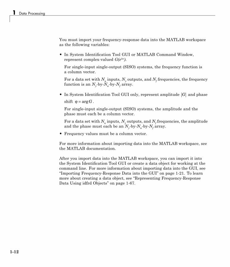
You must import your frequency-response data into the MATLAB workspaceas the following variables:
• In System Identification Tool GUI or MATLAB Command Window,represent complex-valued G(eiw).
For single-input single-output (SISO) systems, the frequency function isa column vector.
For a data set with Nu inputs, Ny outputs, and Nf frequencies, the frequencyfunction is an Ny-by-Nu-by-Nf array.
• In System Identification Tool GUI only, represent amplitude G and phaseshift ϕ = arg G .
For single-input single-output (SISO) systems, the amplitude and thephase must each be a column vector.
For a data set withNu inputs, Ny outputs, and Nf frequencies, the amplitudeand the phase must each be an Ny-by-Nu-by-Nf array.
• Frequency values must be a column vector.
For more information about importing data into the MATLAB workspace, seethe MATLAB documentation.
After you import data into the MATLAB workspace, you can import it intothe System Identification Tool GUI or create a data object for working at thecommand line. For more information about importing data into the GUI, see“Importing Frequency-Response Data into the GUI” on page 1-21. To learnmore about creating a data object, see “Representing Frequency-ResponseData Using idfrd Objects” on page 1-67.
1-12

Representing Data in the GUI
Representing Data in the GUI
In this section...
“Types of Data You Can Import into the GUI” on page 1-13“Importing Time-Domain Data into the GUI” on page 1-15“Importing Frequency-Domain Data into the GUI” on page 1-18“Importing Frequency-Response Data into the GUI” on page 1-21“Importing Data Objects into the GUI” on page 1-25“Specifying the Data Sampling Interval” on page 1-28“Specifying Estimation and Validation Data” on page 1-29“Preprocessing Data Using Quick Start” on page 1-30“Creating Data Sets from a Subset of Signal Channels” on page 1-31“Creating Multiexperiment Data Sets in the GUI” on page 1-33“Viewing Data Properties” on page 1-40“Renaming Data and Changing Display Color” on page 1-41“Distinguishing Data Types in the GUI” on page 1-43“Organizing Data Icons” on page 1-43“Deleting Data Sets in the GUI” on page 1-44“Exporting Data from the GUI to the MATLAB Workspace” on page 1-45
Types of Data You Can Import into the GUIYou can import the following types of data from the MATLAB workspace intothe System Identification Tool GUI:
• “Importing Time-Domain Data into the GUI” on page 1-15
• “Importing Frequency-Domain Data into the GUI” on page 1-18
• “Importing Frequency-Response Data into the GUI” on page 1-21
• “Importing Data Objects into the GUI” on page 1-25
1-13

1 Data Processing
To open the GUI, type the following command in the MATLAB CommandWindow:
ident
In the Import data list, select the type of data to import from the MATLABworkspace, as shown in the following figure.
For an example of importing data into the System Identification Tool GUI, seethe Getting Started documentation.
1-14

Representing Data in the GUI
Importing Time-Domain Data into the GUIBefore you can import time-domain data into the System Identification ToolGUI, you must import the data into the MATLAB workspace, as described in“Importing Time-Domain Data into MATLAB” on page 1-6.
Note Your time-domain data must be sampled at equal time intervals. Theinput and output signals must have the same number of data samples.
To import data into the GUI:
1 Type the following command in the MATLAB Command Window to openthe GUI:
ident
2 In the System Identification Tool window, select Import data > Timedomain data. This action opens the Import Data dialog box.
1-15

1 Data Processing
3 Specify the following options:
Note For time series, only import the output signal and enter [] for theinput.
• Input — Enter the MATLAB variable name (column vector or matrix)or a MATLAB expression that represents the input data. The expressionmust evaluate to a column vector or matrix.
• Output — Enter the MATLAB variable name (column vector ormatrix) or a MATLAB expression that represents the output data. Theexpression must evaluate to a column vector or matrix.
• Data name — Enter the name of the data set, which appears inthe System Identification Tool window after the import operation iscompleted.
• Starting time— Enter the starting value of the time axis for time plots.
• Sampling interval — Enter the actual sampling interval in theexperiment. For more information about this setting, see “Specifying theData Sampling Interval” on page 1-28.
Tip The System Identification Toolbox product uses the samplinginterval during model estimation and to set the horizontal axis on timeplots. If you transform a time-domain signal to a frequency-domainsignal, the Fourier transforms are computed as discrete Fouriertransforms (DFTs) using this sampling interval.
1-16

Representing Data in the GUI
4 (Optional) In the Data Information area, clickMore to expand the dialogbox and enter the following settings:
Input Properties
• InterSample— This setting specifies the behavior of the input signalsbetween samples when you transform the resulting models betweendiscrete-time and continuous-time representations.
– zoh (zero-order hold) maintains a piecewise-constant input signalbetween samples.
– foh (first-order hold) maintains a piecewise-linear input signalbetween samples.
– bl (bandwidth-limited behavior) specifies that the continuous-timeinput signal has zero power above the Nyquist frequency (equal to theinverse of the sampling interval).
Note See the d2c and c2d reference pages for more information abouttransforming between discrete-time and continuous-time models.
• Period— Enter Inf to specify a nonperiodic input. For a periodic input,type the period of the input signal in your experiment.
Note If your data is periodic, always include a whole number of periodsfor model estimation.
Channel Names
• Input — Enter a string to specify the name of one or more inputchannels.
Tip Naming channels helps you to identify data in plots. Formultivariable input-output signals, you can specify the names ofindividual Input and Output channels, separated by commas.
1-17
1 Data Processing
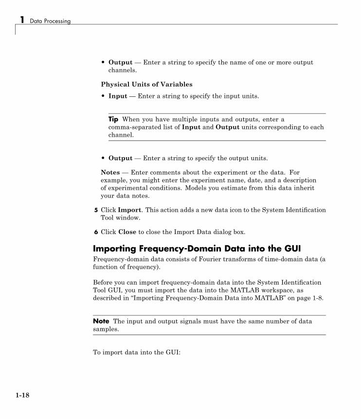
• Output — Enter a string to specify the name of one or more outputchannels.
Physical Units of Variables
• Input — Enter a string to specify the input units.
Tip When you have multiple inputs and outputs, enter acomma-separated list of Input and Output units corresponding to eachchannel.
• Output — Enter a string to specify the output units.
Notes — Enter comments about the experiment or the data. Forexample, you might enter the experiment name, date, and a descriptionof experimental conditions. Models you estimate from this data inherityour data notes.
5 Click Import. This action adds a new data icon to the System IdentificationTool window.
6 Click Close to close the Import Data dialog box.
Importing Frequency-Domain Data into the GUIFrequency-domain data consists of Fourier transforms of time-domain data (afunction of frequency).
Before you can import frequency-domain data into the System IdentificationTool GUI, you must import the data into the MATLAB workspace, asdescribed in “Importing Frequency-Domain Data into MATLAB” on page 1-8.
Note The input and output signals must have the same number of datasamples.
To import data into the GUI:
1-18

Representing Data in the GUI
1 Type the following command in the MATLAB Command Window to openthe GUI:
ident
2 In the System Identification Tool window, select Import data > Freq.domain data. This action opens the Import Data dialog box.
3 Specify the following options:
• Input — Enter the MATLAB variable name (column vector or matrix)or a MATLAB expression that represents the input data. The expressionmust evaluate to a column vector or matrix.
• Output — Enter the MATLAB variable name (column vector ormatrix) or a MATLAB expression that represents the output data. Theexpression must evaluate to a column vector or matrix.
• Frequency — Enter the MATLAB variable name of a vector or aMATLAB expression that represents the frequency. The expressionmust evaluate to a column vector.
The frequency vector must have the same number of rows as the inputand output signals.
• Data name — Enter the name of the data set, which appears inthe System Identification Tool window after the import operation iscompleted.
• Frequency unit— Enter Hz for Hertz or keep the rad/s default value.
• Sampling interval — Enter the actual sampling interval in theexperiment. For continuous-time data, enter 0. For more informationabout this setting, see “Specifying the Data Sampling Interval” on page1-28.
4 (Optional) In the Data Information area, clickMore to expand the dialogbox and enter the following optional settings:
Input Properties
1-19

1 Data Processing
• InterSample— This setting specifies the behavior of the input signalsbetween samples when you transform the resulting models betweendiscrete-time and continuous-time representations.
– zoh (zero-order hold) maintains a piecewise-constant input signalbetween samples.
– foh (first-order hold) maintains a piecewise-linear input signalbetween samples.
– bl (bandwidth-limited behavior) specifies that the continuous-timeinput signal has zero power above the Nyquist frequency (equal to theinverse of the sampling interval).
Note See the d2c and c2d reference page for more information abouttransforming between discrete-time and continuous-time models.
• Period— Enter Inf to specify a nonperiodic input. For a periodic input,type the period of the input signal in your experiment.
Note If your data is periodic, always include a whole number of periodsfor model estimation.
Channel Names
• Input — Enter a string to specify the name of one or more inputchannels.
Tip Naming channels helps you to identify data in plots. Formultivariable input and output signals, you can specify the names ofindividual Input and Output channels, separated by commas.
• Output — Enter a string to specify the name of one or more outputchannels.
Physical Units of Variables
1-20
Representing Data in the GUI
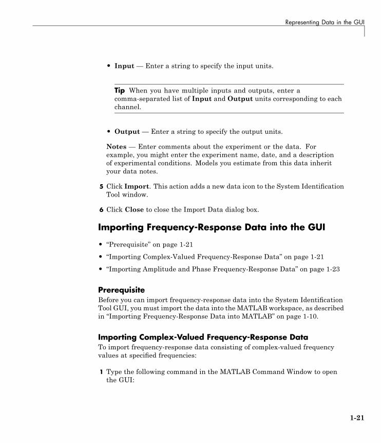
• Input — Enter a string to specify the input units.
Tip When you have multiple inputs and outputs, enter acomma-separated list of Input and Output units corresponding to eachchannel.
• Output — Enter a string to specify the output units.
Notes — Enter comments about the experiment or the data. Forexample, you might enter the experiment name, date, and a descriptionof experimental conditions. Models you estimate from this data inherityour data notes.
5 Click Import. This action adds a new data icon to the System IdentificationTool window.
6 Click Close to close the Import Data dialog box.
Importing Frequency-Response Data into the GUI
• “Prerequisite” on page 1-21
• “Importing Complex-Valued Frequency-Response Data” on page 1-21
• “Importing Amplitude and Phase Frequency-Response Data” on page 1-23
PrerequisiteBefore you can import frequency-response data into the System IdentificationTool GUI, you must import the data into the MATLAB workspace, as describedin “Importing Frequency-Response Data into MATLAB” on page 1-10.
Importing Complex-Valued Frequency-Response DataTo import frequency-response data consisting of complex-valued frequencyvalues at specified frequencies:
1 Type the following command in the MATLAB Command Window to openthe GUI:
1-21

1 Data Processing
ident
2 In the System Identification Tool window, select Import data > Freq.domain data. This action opens the Import Data dialog box.
3 In the Data Format for Signals list, select Freq. Function (Complex).
4 Specify the following options:
• Freq. Func. — Enter the MATLAB variable name or a MATLABexpression that represents the complex frequency-response data G(eiw).
• Frequency — Enter the MATLAB variable name of a vector or aMATLAB expression that represents the frequency. The expressionmust evaluate to a column vector.
• Data name — Enter the name of the data set, which appears inthe System Identification Tool window after the import operation iscompleted.
• Frequency unit— Enter Hz for Hertz or keep the rad/s default value.
• Sampling interval — Enter the actual sampling interval in theexperiment. For continuous-time data, enter 0. For more informationabout this setting, see “Specifying the Data Sampling Interval” on page1-28.
5 (Optional) In the Data Information area, clickMore to expand the dialogbox and enter the following optional settings:
Channel Names
• Input — Enter a string to specify the name of one or more inputchannels.
Tip Naming channels helps you to identify data in plots. Formultivariable input and output signals, you can specify the names ofindividual Input and Output channels, separated by commas.
• Output — Enter a string to specify the name of one or more outputchannels.
1-22
Representing Data in the GUI
Physical Units of Variables
• Input — Enter a string to specify the input units.
Tip When you have multiple inputs and outputs, enter acomma-separated list of Input and Output units corresponding to eachchannel.
• Output — Enter a string to specify the output units.
Notes — Enter comments about the experiment or the data. Forexample, you might enter the experiment name, date, and a descriptionof experimental conditions. Models you estimate from this data inherityour data notes.
6 Click Import. This action adds a new data icon to the System IdentificationTool window.
7 Click Close to close the Import Data dialog box.
Importing Amplitude and Phase Frequency-Response DataTo import frequency-response data consisting of amplitude and phase valuesat specified frequencies:
1 Type the following command in the MATLAB Command Window to openthe GUI:
ident
2 In the System Identification Tool window, select Import data > Freq.domain data. This action opens the Import Data dialog box.
3 In the Data Format for Signals list, select Freq. Function(Amp/Phase).
1-23
1 Data Processing
4 Specify the following options:
• Amplitude — Enter the MATLAB variable name or a MATLAB
expression that represents the amplitude G .
• Phase (deg) — Enter the MATLAB variable name or a MATLABexpression that represents the phase ϕ = arg G .
• Frequency — Enter the MATLAB variable name of a vector or aMATLAB expression that represents the frequency. The expressionmust evaluate to a column vector.
• Data name — Enter the name of the data set, which appears inthe System Identification Tool window after the import operation iscompleted.
• Frequency unit— Enter Hz for Hertz or keep the rad/s default value.
• Sampling interval — Enter the actual sampling interval in theexperiment. For continuous-time data, enter 0. For more informationabout this setting, see “Specifying the Data Sampling Interval” on page1-28.
5 (Optional) In the Data Information area, clickMore to expand the dialogbox and enter the following optional settings:
Channel Names
• Input — Enter a string to specify the name of one or more inputchannels.
Tip Naming channels helps you to identify data in plots. Formultivariable input and output signals, you can specify the names ofindividual Input and Output channels, separated by commas.
• Output — Enter a string to specify the name of one or more outputchannels.
Physical Units of Variables
• Input — Enter a string to specify the input units.
1-24
Representing Data in the GUI
Tip When you have multiple inputs and outputs, enter acomma-separated list of Input and Output units corresponding to eachchannel.
• Output — Enter a string to specify the output units.
Notes — Enter comments about the experiment or the data. Forexample, you might enter the experiment name, date, and a descriptionof experimental conditions. Models you estimate from this data inherityour data notes.
6 Click Import. This action adds a new data icon to the System IdentificationTool window.
7 Click Close to close the Import Data dialog box.
Importing Data Objects into the GUIYou can import the System Identification Toolbox iddata and idfrd dataobjects into the System Identification Tool GUI.
Before you can import a data object into the System Identification Tool GUI,you must create the data object in the MATLAB workspace, as described in“Representing Time- and Frequency-Domain Data Using iddata Objects” onpage 1-47 or “Representing Frequency-Response Data Using idfrd Objects”on page 1-67.
Note You can also import a Control System Toolbox™ frd object. Importingan frd object converts it to an idfrd object.
Select Import data > Data object to open the Import Data dialog box.
Import iddata, idfrd, or frd data object in the MATLAB workspace.
To import a data object into the GUI:
1-25

1 Data Processing
1 Type the following command in the MATLAB Command Window to openthe GUI:
ident
2 In the System Identification Tool window, select Import data > Dataobject.
This action opens the Import Data dialog box. IDDATA or IDFRD/FRD isalready selected in the Data Format for Signals list.
3 Specify the following options:
• Object— Enter the name of the MATLAB variable that represents thedata object in the MATLAB workspace. Press Enter.
• Data name — Enter the name of the data set, which appears inthe System Identification Tool window after the import operation iscompleted.
• Starting time— Enter the starting value of the time axis for time plots.
• Sampling interval — Enter the actual sampling interval in theexperiment. For more information about this setting, see “Specifying theData Sampling Interval” on page 1-28.
Tip The System Identification Toolbox product uses the samplinginterval during model estimation and to set the horizontal axis on timeplots. If you transform a time-domain signal to a frequency-domainsignal, the Fourier transforms are computed as discrete Fouriertransforms (DFTs) using this sampling interval.
1-26

Representing Data in the GUI
4 (Optional) In the Data Information area, clickMore to expand the dialogbox and enter the following optional settings:
Input Properties
• InterSample— This setting specifies the behavior of the input signalsbetween samples when you transform the resulting models betweendiscrete-time and continuous-time representations.
– zoh (zero-order hold) maintains a piecewise-constant input signalbetween samples.
– foh (first-order hold) maintains a piecewise-linear input signalbetween samples.
– bl (bandwidth-limited behavior) specifies that the continuous-timeinput signal has zero power above the Nyquist frequency (equal to theinverse of the sampling interval).
Note See the d2c and c2d reference page for more information abouttransforming between discrete-time and continuous-time models.
• Period— Enter Inf to specify a nonperiodic input. For a periodic input,type the period of the input signal in your experiment.
Note If your data is periodic, always include a whole number of periodsfor model estimation.
Channel Names
• Input — Enter a string to specify the name of one or more inputchannels.
Tip Naming channels helps you to identify data in plots. Formultivariable input and output signals, you can specify the names ofindividual Input and Output channels, separated by commas.
1-27
1 Data Processing
• Output — Enter a string to specify the name of one or more outputchannels.
Physical Units of Variables
• Input — Enter a string to specify the input units.
Tip When you have multiple inputs and outputs, enter acomma-separated list of Input and Output units corresponding to eachchannel.
• Output — Enter a string to specify the output units.
Notes — Enter comments about the experiment or the data. Forexample, you might enter the experiment name, date, and a descriptionof experimental conditions. Models you estimate from this data inherityour data notes.
5 Click Import. This action adds a new data icon to the System IdentificationTool window.
6 Click Close to close the Import Data dialog box.
Specifying the Data Sampling IntervalWhen you import data into the GUI, you must specify the data samplinginterval.
The sampling interval is the time between successive data samples in yourexperiment and must be the numerical time interval at which your data issampled in any units. For example, enter 0.5 if your data was sampled every0.5 s, and enter 1 if your data was sampled every 1 s.
You can also use the sampling interval as a flag to specify continuous-timedata. When importing continuous-time frequency domain orfrequency-response data, set the Sampling interval to 0.
The sampling interval is used during model estimation. For time-domaindata, the sampling interval is used together with the start time to calculatethe sampling time instants. When you transform time-domain signals to
1-28

Representing Data in the GUI
frequency-domain signals (see the fft reference page), the Fourier transformsare computed as discrete Fourier transforms (DFTs) for this samplinginterval. In addition, the sampling instants are used to set the horizontalaxis on time plots.
Sampling Interval in the Import Data dialog box
Specifying Estimation and Validation DataTo avoid overfitting, you should use independent data sets to estimate andvalidate your model.
In the System Identification Tool GUI, Working Data refers to estimationdata. Similarly, Validation Data refers to the data set you use to validate amodel. For example, when you plot the model output and residual-analysisplots, the input to the model is the input signal from the validation data set.These plots compare model output to the measured output in the validationdata set.
To specifyWorking Data, drag and drop the corresponding data icon into theWorking Data rectangle, as shown in the following figure.
1-29

1 Data Processing
Similarly, to specify Validation Data, drag and drop the corresponding dataicon into the Validation Data rectangle.
Preprocessing Data Using Quick StartAs a preprocessing shortcut, select Preprocess > Quick start tosimultaneously perform the following four actions:
• Subtract the mean value from each channel.
Note For information about when to subtract mean values from the data,see “Subtracting Trends from Signals (Detrending)” on page 1-94.
• Split data into two parts.
• Specify the first part as estimation data for models (orWorking Data).
• Specify the second part as Validation Data.
1-30

Representing Data in the GUI
Creating Data Sets from a Subset of Signal ChannelsYou can create a new data set in the System Identification Tool GUI byextracting subsets of input and output channels from an existing data set.
To create a new data set from selected channels:
1 In the System Identification Tool GUI, drag the icon of the data from whichyou want to select channels to the Working Data rectangle.
2 Select Preprocess > Select channels to open the Select Channels dialogbox.
The Inputs list displays the input channels and the Outputs list displaysthe output channels in the selected data set.
1-31
1 Data Processing
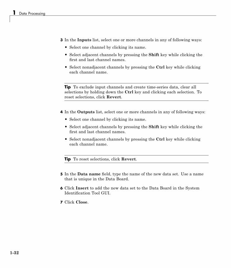
3 In the Inputs list, select one or more channels in any of following ways:
• Select one channel by clicking its name.
• Select adjacent channels by pressing the Shift key while clicking thefirst and last channel names.
• Select nonadjacent channels by pressing the Ctrl key while clickingeach channel name.
Tip To exclude input channels and create time-series data, clear allselections by holding down the Ctrl key and clicking each selection. Toreset selections, click Revert.
4 In the Outputs list, select one or more channels in any of following ways:
• Select one channel by clicking its name.
• Select adjacent channels by pressing the Shift key while clicking thefirst and last channel names.
• Select nonadjacent channels by pressing the Ctrl key while clickingeach channel name.
Tip To reset selections, click Revert.
5 In the Data name field, type the name of the new data set. Use a namethat is unique in the Data Board.
6 Click Insert to add the new data set to the Data Board in the SystemIdentification Tool GUI.
7 Click Close.
1-32
Representing Data in the GUI
Creating Multiexperiment Data Sets in the GUI
• “Why Create Multiexperiment Data?” on page 1-33
• “Limitations on Data Sets” on page 1-33
• “Merging Data Sets” on page 1-33
• “Extracting Specific Experiments from a Multiexperiment Data Set into aNew Data Set” on page 1-37
Why Create Multiexperiment Data?You can create a time-domain or frequency-domain data set in the SystemIdentification Tool GUI that includes several experiments. Identifying modelsfor multiexperiment data results in an average model.
Experiments can mean data that was collected during different sessions, orportions of the data collected during a single session. In the latter situation,you can create multiexperiment data by splitting a single data set intomultiple segments that exclude corrupt data, and then merge the good datasegments.
Limitations on Data SetsYou can only merge data sets that have all of the following characteristics:
• Same number of input and output channels.
• Different names. The name of each data set becomes the experiment namein the merged data set.
• Same input and output channel names.
• Same data domain (that is, time-domain data or frequency-domain dataonly).
Merging Data SetsYou can merge data sets using the System Identification Tool GUI.
1-33

1 Data Processing
Note Before merging several segments of the same data set, verify thatthe time vector of each data starts at the time when that data segment wasactually measured (relative to the other data sets).
For example, suppose that you want to combine the data sets tdata, tdata2,tdata3, tdata4 shown in the following figure.
GUI Contains Four Data Sets to Merge
1-34

Representing Data in the GUI
To merge data sets in the GUI:
1 In the Operations area, select <–Preprocess > Merge experimentsfrom the drop-down menu to open the Merge Experiments dialog box.
1-35
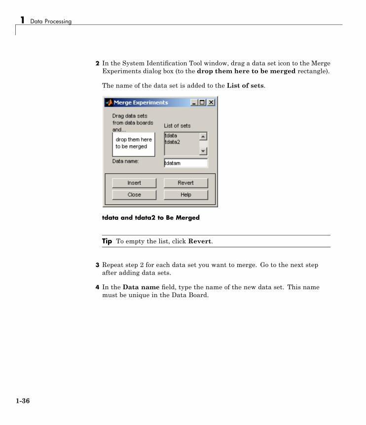
1 Data Processing
2 In the System Identification Tool window, drag a data set icon to the MergeExperiments dialog box (to the drop them here to be merged rectangle).
The name of the data set is added to the List of sets.
tdata and tdata2 to Be Merged
Tip To empty the list, click Revert.
3 Repeat step 2 for each data set you want to merge. Go to the next stepafter adding data sets.
4 In the Data name field, type the name of the new data set. This namemust be unique in the Data Board.
1-36
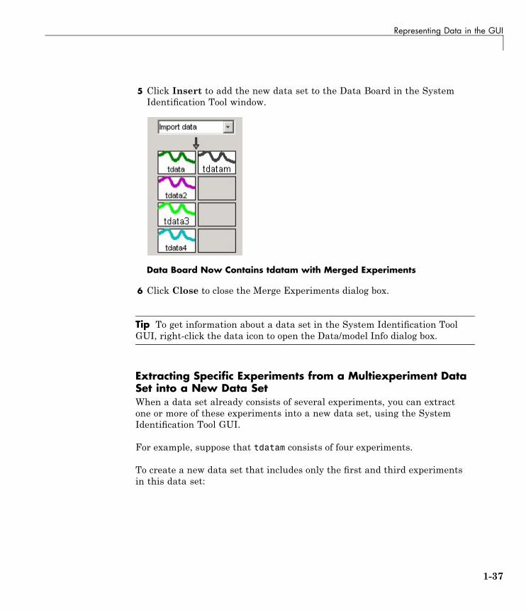
Representing Data in the GUI
5 Click Insert to add the new data set to the Data Board in the SystemIdentification Tool window.
Data Board Now Contains tdatam with Merged Experiments
6 Click Close to close the Merge Experiments dialog box.
Tip To get information about a data set in the System Identification ToolGUI, right-click the data icon to open the Data/model Info dialog box.
Extracting Specific Experiments from a Multiexperiment DataSet into a New Data SetWhen a data set already consists of several experiments, you can extractone or more of these experiments into a new data set, using the SystemIdentification Tool GUI.
For example, suppose that tdatam consists of four experiments.
To create a new data set that includes only the first and third experimentsin this data set:
1-37
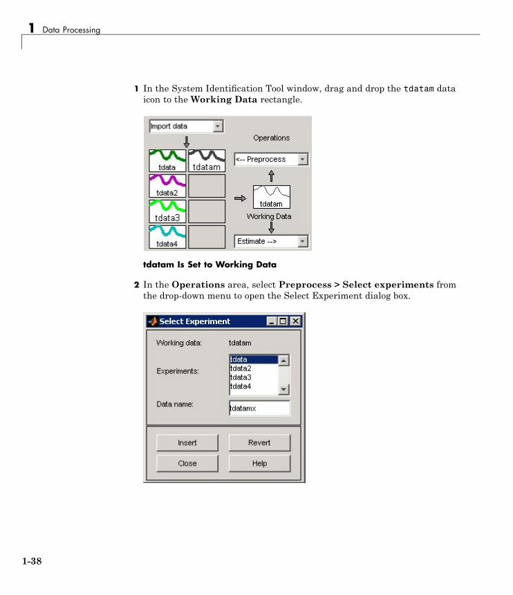
1 Data Processing
1 In the System Identification Tool window, drag and drop the tdatam dataicon to the Working Data rectangle.
tdatam Is Set to Working Data
2 In the Operations area, select Preprocess > Select experiments fromthe drop-down menu to open the Select Experiment dialog box.
1-38
Representing Data in the GUI
3 In the Experiments list, select one or more data sets in either of thefollowing ways:
• Select one data set by clicking its name.
• Select adjacent data sets by pressing the Shift key while clicking thefirst and last names.
• Select nonadjacent data sets by pressing the Ctrl key while clickingeach name.
4 In the Data name field, type the name of the new data set. This namemust be unique in the Data Board.
5 Click Insert to add the new data set to the Data Board in the SystemIdentification Tool GUI.
6 Click Close to close the Select Experiment dialog box.
1-39
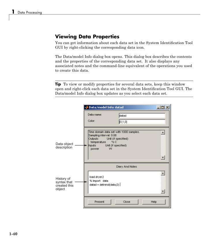
1 Data Processing
Viewing Data PropertiesYou can get information about each data set in the System Identification ToolGUI by right-clicking the corresponding data icon.
The Data/model Info dialog box opens. This dialog box describes the contentsand the properties of the corresponding data set. It also displays anyassociated notes and the command-line equivalent of the operations you usedto create this data.
Tip To view or modify properties for several data sets, keep this windowopen and right-click each data set in the System Identification Tool GUI. TheData/model Info dialog box updates as you select each data set.
����������� ������
����� ��������������� ������������
1-40

Representing Data in the GUI
To displays the data properties in the MATLAB Command Window, clickPresent.
Renaming Data and Changing Display ColorYou can rename data and change its display color by double-clicking the dataicon in the System Identification Tool GUI.
The Data/model Info dialog box opens. This dialog box describes both thecontents and the properties of the data. The object description area displaysthe syntax of the operations you used to create the data in the GUI.
The Data/model Info dialog box also lets you rename the data by entering anew name in the Data name field.
You can also specify a new display color using three RGB values in the Colorfield. Each value is between 0 to 1 and indicates the relative presence ofred, green, and blue, respectively. For more information about specifyingdefault data color, see “Customizing the System Identification Tool GUI” onpage 12-21.
Tip As an alternative to using three RGB values, you can enter any one ofthe following letters in single quotes:
'y' 'r' 'b' 'c' 'g' 'm' 'k'
These strings represent yellow, red, blue, cyan, green, magenta, and black,respectively.
1-41

1 Data Processing
����������� ������
����� ��������������� ������������
Information About the Data
You can enter comments about the origin and state of the data in the DiaryAnd Notes area. For example, you might want to include the experimentname, date, and the description of experimental conditions. When youestimate models from this data, these notes are associated with the models.
Clicking Present display the portions of this information in the MATLABCommand Window.
1-42
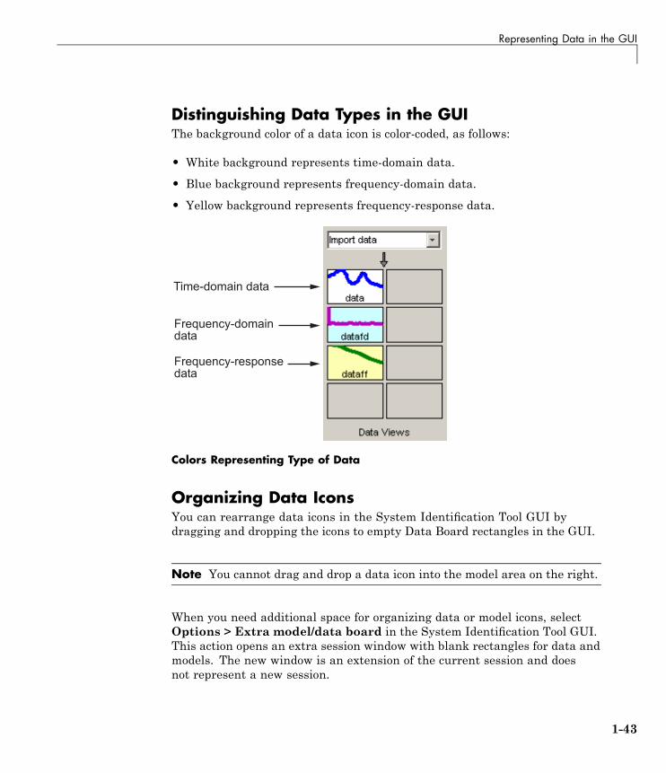
Representing Data in the GUI
Distinguishing Data Types in the GUIThe background color of a data icon is color-coded, as follows:
• White background represents time-domain data.
• Blue background represents frequency-domain data.
• Yellow background represents frequency-response data.
���������������
� ���������������
� ����� ���������
Colors Representing Type of Data
Organizing Data IconsYou can rearrange data icons in the System Identification Tool GUI bydragging and dropping the icons to empty Data Board rectangles in the GUI.
Note You cannot drag and drop a data icon into the model area on the right.
When you need additional space for organizing data or model icons, selectOptions > Extra model/data board in the System Identification Tool GUI.This action opens an extra session window with blank rectangles for data andmodels. The new window is an extension of the current session and doesnot represent a new session.
1-43
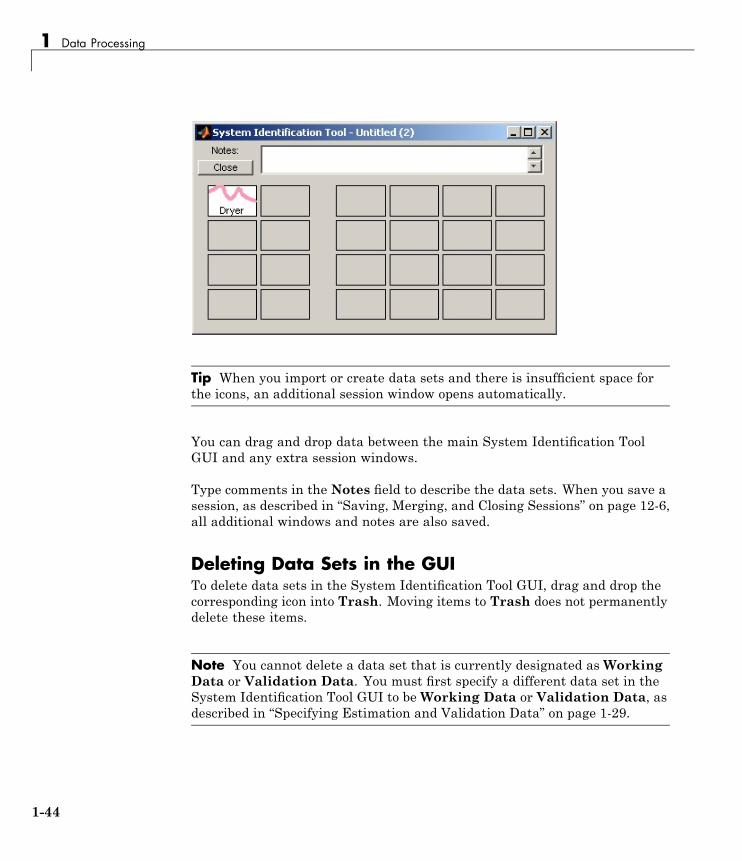
1 Data Processing
Tip When you import or create data sets and there is insufficient space forthe icons, an additional session window opens automatically.
You can drag and drop data between the main System Identification ToolGUI and any extra session windows.
Type comments in the Notes field to describe the data sets. When you save asession, as described in “Saving, Merging, and Closing Sessions” on page 12-6,all additional windows and notes are also saved.
Deleting Data Sets in the GUITo delete data sets in the System Identification Tool GUI, drag and drop thecorresponding icon into Trash. Moving items to Trash does not permanentlydelete these items.
Note You cannot delete a data set that is currently designated asWorkingData or Validation Data. You must first specify a different data set in theSystem Identification Tool GUI to beWorking Data or Validation Data, asdescribed in “Specifying Estimation and Validation Data” on page 1-29.
1-44

Representing Data in the GUI
To restore a data set from Trash, drag its icon from Trash to the Data orModel Board in the System Identification Tool window. You can view theTrash contents by double-clicking the Trash icon.
Note You must restore data to the Data Board; you cannot drag data icons tothe Model Board.
To permanently delete all items in Trash, select Options > Empty trash.
Exiting a session empties the Trash automatically.
Exporting Data from the GUI to the MATLABWorkspaceThe data you create in the System Identification Tool GUI is not availablein the MATLAB workspace until you export the data set. Exporting to theMATLAB workspace is necessary when you need to perform an operation onthe data that is only available at the command line.
To export a data set to the MATLAB workspace, drag and drop thecorresponding icon to the To Workspace rectangle.
1-45
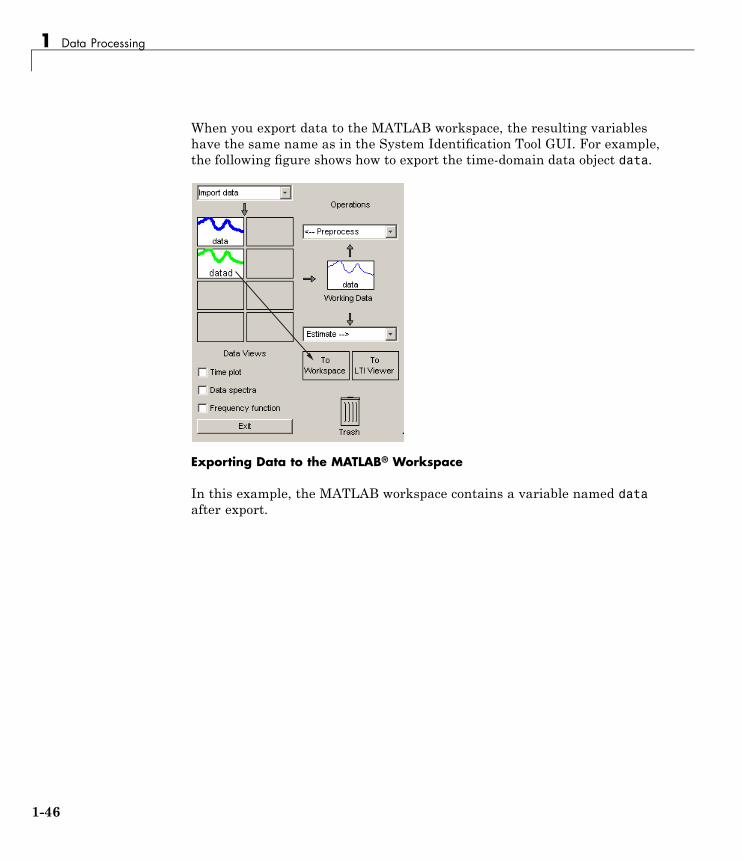
1 Data Processing
When you export data to the MATLAB workspace, the resulting variableshave the same name as in the System Identification Tool GUI. For example,the following figure shows how to export the time-domain data object data.
Exporting Data to the MATLAB® Workspace
In this example, the MATLAB workspace contains a variable named dataafter export.
1-46
Representing Time- and Frequency-Domain Data Using iddata Objects
Representing Time- and Frequency-Domain Data Usingiddata Objects
In this section...
“iddata Constructor” on page 1-47“iddata Properties” on page 1-50“Creating Multiexperiment Data at the Command Line” on page 1-53“Subreferencing iddata Objects” on page 1-55“Modifying Time and Frequency Vectors” on page 1-59“Naming, Adding, and Removing Data Channels” on page 1-63“Concatenating iddata Objects” on page 1-65
iddata Constructor
• “Requirements for Constructing an iddata Object” on page 1-47
• “Constructing an iddata Object for Time-Domain Data” on page 1-48
• “Constructing an iddata Object for Frequency-Domain Data” on page 1-49
Requirements for Constructing an iddata ObjectTo construct an iddata object, you must have already imported data into theMATLAB workspace, as described in “Importing Data into the MATLABWorkspace” on page 1-5.
1-47
1 Data Processing
Constructing an iddata Object for Time-Domain DataUse the following syntax to create a time-domain iddata object data:
data = iddata(y,u,Ts)
You can also specify additional properties, as follows:
data = iddata(y,u,Ts,'Property1',Value1,...,'PropertyN',ValueN)
For more information about accessing object properties, see “iddataProperties” on page 1-50.
In this example, Ts is the sampling time, or the time interval, betweensuccessive data samples. For uniformly sampled data, Ts is a scalar valueequal to the sampling interval of your experiment. The default time unit isseconds, but you can specify any unit string using the TimeUnit property.For more information about iddata time properties, see “Modifying Timeand Frequency Vectors” on page 1-59.
For nonuniformly sampled data, specify Ts as [], and set the value of theSamplingInstants property as a column vector containing individual timevalues. For example:
data = iddata(y,u,Ts,[],'SamplingInstants',TimeVector)
Where TimeVector represents a vector of time values.
Note You can modify the property SamplingInstants by setting it to a newvector with the length equal to the number of data samples.
To represent time-series data, use the following syntax:
ts_data = iddata(y,[],Ts)
where y is the output data, [] indicates empty input data, and Ts is thesampling interval.
1-48

Representing Time- and Frequency-Domain Data Using iddata Objects
The following example shows how to create an iddata object usingsingle-input/single-output (SISO) data from dryer2.mat. The input andoutput each contain 1000 samples with the sampling interval of 0.08 second.
load dryer2 % Load input u2 and output y2.data = iddata(y2,u2,0.08) % Create iddata object.
MATLAB returns the following output:
Time domain data set with 1000 samples.Sampling interval: 0.08
Outputs Unit (if specified)y1
Inputs Unit (if specified)u1
The default channel name 'y1' is assigned to the first and only outputchannel. When y2 contains several channels, the channels are assigneddefault names 'y1','y2','y2',...,'yn'. Similarly, the default channelname 'u1' is assigned to the first and only output channel. For moreinformation about naming channels, see “Naming, Adding, and RemovingData Channels” on page 1-63.
Constructing an iddata Object for Frequency-Domain DataFrequency-domain data is the Fourier transform of the input and outputsignals at specific frequency values. To represent frequency-domain data, usethe following syntax to create the iddata object:
data = iddata(y,u,Ts,'Frequency',w)
'Frequency' is an iddata property that specifies the frequency values w,where w is the frequency column vector that defines the frequencies forcalculating the Fourier transform values of y and u. Ts is the time intervalbetween successive data samples in seconds. w, y, and u have the samenumber of rows.
1-49

1 Data Processing
Note You must specify the frequency vector for frequency-domain data.
For more information about iddata time and frequency properties, see“Modifying Time and Frequency Vectors” on page 1-59.
To specify a continuous-time system, set Ts to 0.
You can specify additional properties when you create the iddata object, asfollows:
data = iddata(y,u,Ts,'Property1',Value1,...,'PropertyN',ValueN)
For more information about accessing object properties, see “iddataProperties” on page 1-50.
iddata PropertiesTo view the properties of the iddata object, use the get command. Forexample, type the following commands at the prompt:
load dryer2 % Load input u2 and output y2data = iddata(y2,u2,0.08); % Create iddata objectget(data) % Get property values of data
1-50

Representing Time- and Frequency-Domain Data Using iddata Objects
MATLAB returns the following object properties and values:
Domain: 'Time'Name: []
OutputData: [1000x1 double]y: 'Same as OutputData'
OutputName: {'y1'}OutputUnit: {''}InputData: [1000x1 double]
u: 'Same as InputData'InputName: {'u1'}InputUnit: {''}
Period: InfInterSample: 'zoh'
Ts: 0.0800Tstart: []
SamplingInstants: [1000x0 double]TimeUnit: ''
ExperimentName: 'Exp1'Notes: []
UserData: []
For a complete description of all properties, see the iddata reference page ortype idprops iddata at the prompt.
You can specify properties when you create an iddata object using theconstructor syntax:
data = iddata(y,u,Ts,'Property1',Value1,...,'PropertyN',ValueN)
To change property values for an existing iddata object, use the set commandor dot notation. For example, to change the sampling interval to 0.05, typethe following at the prompt:
set(data,'Ts',0.05)
or equivalently:
data.ts = 0.05
Property names are not case sensitive. You do not need to type the entireproperty name if the first few letters uniquely identify the property.
1-51

1 Data Processing
Tip You can use data.y as an alternative to data.OutputData to access theoutput values, or use data.u as an alternative to data.InputData to accessthe input values.
An iddata object containing frequency-domain data includesfrequency-specific properties, such as Frequency for the frequency vector andUnits for frequency units (instead of Tstart and SamplingIntervals).
To view the property list, type the following command sequence at the prompt:
% Load input u2 and output y2load dryer2;
% Create iddata objectdata = iddata(y2,u2,0.08);
% Take the Fourier transform of the data% transforming it to frequency domain
data = fft(data)% Get property values of data
get(data)
1-52

Representing Time- and Frequency-Domain Data Using iddata Objects
MATLAB returns the following object properties and values:
Domain: 'Frequency'Name: []
OutputData: [501x1 double]y: 'Same as OutputData'
OutputName: {'y1'}OutputUnit: {''}InputData: [501x1 double]
u: 'Same as InputData'InputName: {'u1'}InputUnit: {''}
Period: InfInterSample: 'zoh'
Ts: 0.0800Units: 'rad/s'
Frequency: [501x1 double]TimeUnit: ''
ExperimentName: 'Exp1'Notes: []
UserData: []
Creating Multiexperiment Data at the Command Line
• “Why Create Multiexperiment Data Sets?” on page 1-53
• “Limitations on Data Sets” on page 1-54
• “Merging Data Sets” on page 1-54
• “Adding Experiments to an Existing iddata Object” on page 1-54
Why Create Multiexperiment Data Sets?You can create iddata objects that contain several experiments. Identifyingmodels for an iddata object with multiple experiments results in an averagemodel.
In the System Identification Toolbox product, experiments can eithermean data collected during different sessions, or portions of the datacollected during a single session. In the latter situation, you can create a
1-53

1 Data Processing
multiexperiment iddata object by splitting the data from a single session intomultiple segments to exclude bad data, and merge the good data portions.
Note The idfrd object does not support the iddata equivalent ofmultiexperiment data.
Limitations on Data SetsYou can only merge data sets that have all of the following characteristics:
• Same number of input and output channels.
• Same input and output channel names.
• Same data domain (that is, time-domain data or frequency-domain data).
Merging Data SetsCreate a multiexperiment iddata object by merging iddata objects, whereeach contains data from a single experiment or is a multiexperiment data set.For example, you can use the following syntax to merge data:
load iddata1 % Loads iddata object z1load iddata3 % Loads iddata object z3z = merge(z1,z3) % Merges experiments z1 and z3 into
% the iddata object z
These commands create an iddata object that conatains two experiments,where the experiments are assigned default names 'Exp1' and 'Exp2',respectively.
Adding Experiments to an Existing iddata ObjectYou can add experiments individually to an iddata object as an alternativeapproach to merging data sets.
For example, to add the experiments in the iddata object dat4 to data, usethe following syntax:
data(:,:,:,'Run4') = dat4
1-54

Representing Time- and Frequency-Domain Data Using iddata Objects
This syntax explicitly assigns the experiment name 'Run4' to the newexperiment. The ExperimentName property of the iddata object storesexperiment names.
For more information about subreferencing experiments in a multiexperimentdata set, see “Subreferencing Experiments” on page 1-58.
Subreferencing iddata Objects
• “Subreferencing Input and Output Data” on page 1-55
• “Subreferencing Data Channels” on page 1-56
• “Subreferencing Experiments” on page 1-58
Subreferencing Input and Output DataSubreferencing data and its properties lets you select data values and assignnew data and property values.
Use the following general syntax to subreference specific data values iniddata objects:
data(samples,outputchannels,inputchannels,experimentname)
In this syntax, samples specify one or more sample indexes, outputchannelsand inputchannels specify channel indexes or channel names, andexperimentname specifies experiment indexes or names.
For example, to retrieve samples 5 through 30 in the iddata object data andstore them in a new iddata object data_sub, use the following syntax:
data_sub = data([5:30])
You can also use logical expressions to subreference data. For example, toretrieve all data values that fall between sample instants 1.27 and 9.3 in theiddata object data and assign them to data_sub, use the following syntax:
data_sub = data(data.sa>1.27&data.sa<9.3)
1-55
1 Data Processing
Note You do not need to type the entire property name. In this example, sain data.sa uniquely identifies the SamplingInstants property.
You can retrieve the input signal from an iddata object using the followingcommands:
u = get(data,'InputData')
or
data.InputData
or
data.u % u is the abbreviation for InputData
Similarly, you can retrieve the output data using
data.OutputData
or
data.y % y is the abbreviation for OutputData
Subreferencing Data ChannelsUse the following general syntax to subreference specific data channels iniddata objects:
data(samples,outputchannels,inputchannels,experimentname)
In this syntax, samples specify one or more sample indexes, outputchannelsand inputchannels specify channel indexes or channel names, andexperimentname specifies experiment indexes or names.
To specify several channel names, you must use a cell array of name strings.
1-56

Representing Time- and Frequency-Domain Data Using iddata Objects
For example, suppose the iddata object data contains three output channels(named y1, y2, and y3), and four input channels (named u1, u2, u3, and u4).To select all data samples in y3, u1, and u4, type the following command atthe prompt:
% Use a cell array to reference% input channels 'u1' and 'u4'data_sub = data(:,'y3',{'u1','u4'})
or equivalently
% Use channel indexes 1 and 4% to reference the input channels
data_sub = data(:,3,[1 4])
Tip Use a colon (:) to specify all samples or all channels, and the emptymatrix ([]) to specify no samples or no channels.
If you want to create a time-series object by extracting only the output datafrom an iddata object, type the following command:
data_ts = data(:,:,[])
You can assign new values to subreferenced variables. For example, thefollowing command assigns the first 10 values of output channel 1 of data tovalues in samples 101 through 110 in the output channel 2 of data1. It alsoassigns the first 10 values of input channel 1 of data to values in samples 101through 110 in the input channel 3 of data1.
data(1:10,1,1) = data1(101:110,2,3)
1-57

1 Data Processing
Subreferencing ExperimentsUse the following general syntax to subreference specific experiments iniddata objects:
data(samples,outputchannels,inputchannels,experimentname)
In this syntax, samples specify one or more sample indexes, outputchannelsand inputchannels specify channel indexes or channel names, andexperimentname specifies experiment indexes or names.
When specifying several experiment names, you must use a cell array of namestrings. The iddata object stores experiments name in the ExperimentNameproperty.
For example, suppose the iddata object data contains five experiments withdefault names, Exp1, Exp2, Exp3, Exp4, and Exp5. Use the following syntax tosubreference the first and fifth experiment in data:
data_sub = data(:,:,:,{'Exp1','Exp5'}) % Using experiment name
or
data_sub = data(:,:,:,[1 5]) % Using experiment index
Tip Use a colon (:) to denote all samples and all channels, and the emptymatrix ([]) to specify no samples and no channels.
Alternatively, you can use the getexp command. The following exampleshows how to subreference the first and fifth experiment in data:
data_sub = getexp(data,{'Exp1','Exp5'}) % Using experiment name
or
data_sub = getexp(data,[1 5]) % Using experiment index
The following example shows how to retrieve the first 100 samples of outputchannels 2 and 3 and input channels 4 to 8 of Experiment 3:
dat(1:100,[2,3],[4:8],3)
1-58
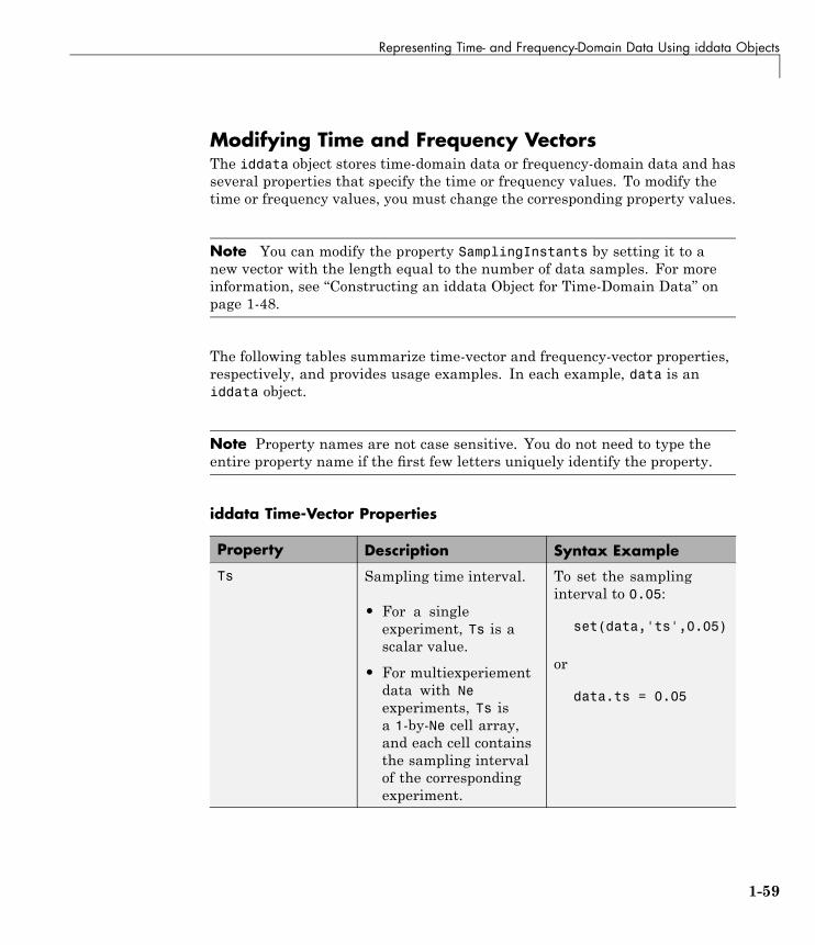
Representing Time- and Frequency-Domain Data Using iddata Objects
Modifying Time and Frequency VectorsThe iddata object stores time-domain data or frequency-domain data and hasseveral properties that specify the time or frequency values. To modify thetime or frequency values, you must change the corresponding property values.
Note You can modify the property SamplingInstants by setting it to anew vector with the length equal to the number of data samples. For moreinformation, see “Constructing an iddata Object for Time-Domain Data” onpage 1-48.
The following tables summarize time-vector and frequency-vector properties,respectively, and provides usage examples. In each example, data is aniddata object.
Note Property names are not case sensitive. You do not need to type theentire property name if the first few letters uniquely identify the property.
iddata Time-Vector Properties
Property Description Syntax Example
Ts Sampling time interval.
• For a singleexperiment, Ts is ascalar value.
• For multiexperiementdata with Neexperiments, Ts isa 1-by-Ne cell array,and each cell containsthe sampling intervalof the correspondingexperiment.
To set the samplinginterval to 0.05:
set(data,'ts',0.05)
or
data.ts = 0.05
1-59

1 Data Processing
iddata Time-Vector Properties (Continued)
Property Description Syntax Example
Tstart Starting time of theexperiment.
• For a singleexperiment, Ts is ascalar value.
• For multiexperiementdata with Neexperiments, Ts isa 1-by-Ne cell array,and each cell containsthe sampling intervalof the correspondingexperiment.
To change starting timeof the first data sample to24:
data.Tstart = 24
Time units are set by theproperty TimeUnit.
1-60

Representing Time- and Frequency-Domain Data Using iddata Objects
iddata Time-Vector Properties (Continued)
Property Description Syntax Example
SamplingInstants Time values in the timevector, computed from theproperties Tstart and Ts.
• For a singleexperiment,SamplingInstantsis an N-by-1 vector.
• For multiexperiementdata with Neexperiments, thisproperty is a 1-by-Necell array, and eachcell contains thesampling instantsof the correspondingexperiment.
To retrieve the timevector for iddata objectdata, use:
get(data,'sa')
To plot the input data asa function of time:
plot(data.sa,data.u)
Note sa is the firsttwo letters of theSamplingInstantsproperty that uniquelyidentifies this property.
TimeUnit Unit of time. To change the unit of thetime vector to msec:
data.ti = 'msec'
1-61

1 Data Processing
iddata Frequency-Vector Properties
Property Description Syntax Example
Frequency Frequency values atwhich the Fouriertransforms of the signalsare defined.
• For a singleexperiment, Frequencyis a scalar value.
• For multiexperiementdata with Neexperiments,Frequency is a1-by-Ne cell array,and each cell containsthe frequencies ofthe correspondingexperiment.
To specify 100 frequencyvalues in log space,ranging between 0.1 and100, use the followingsyntax:
data.freq =logspace(-1,2,100)
Units Frequency unit musthave the following values:
• If the TimeUnit isempty or s (seconds),enter rad/s or Hz
• If the TimeUnit is anystring unit (other thans), enter rad/unit.
For multiexperiementdata with Ne experiments,Units is a 1-by-Ne cellarray, and each cellcontains the frequencyunit for each experiment.
If you specified theTimeUnit as msec, yourfrequency units must be:
data.unit='rad/msec'
1-62

Representing Time- and Frequency-Domain Data Using iddata Objects
Naming, Adding, and Removing Data Channels
• “What Are Input and Output Channels?” on page 1-63
• “Naming Channels” on page 1-63
• “Adding Channels” on page 1-64
• “Modifying Channel Data” on page 1-64
What Are Input and Output Channels?A multivariate system might contain several input variables or several outputvariables, or both. When an input or output signal includes several measuredvariables, these variables are called channels.
Naming ChannelsThe iddata properties InputName and OutputName store one or more channelnames for the input and output signals. When you plot the data, you usechannel names to select the variable displayed on the plot. If you havemultivariate data, you should assign a name to each channel that describesthe measured variable. For more information about selecting channels on aplot, see “Selecting Measured and Noise Channels in Plots” on page 12-18.
You can use the set command to specify the names of individual channels.For example, suppose data contains two input channels (voltage and current)and one output channel (temperature). To set these channel names, use thefollowing syntax:
set(data,'InputName',{'Voltage','Current'},'OutputName','Temperature')
Tip You can also specify channel names as follows:
data.una = {'Voltage','Current')data.yna = 'Temperature'
una is equivalent to the property InputName, and yna is equivalent toOutputName.
1-63

1 Data Processing
If you do not specify channel names when you create the iddata object,the toolbox assigns default names. By default, the output channelsare named 'y1','y2',...,'yn', and the input channels are named'u1','u2',...,'un'.
Adding ChannelsYou can add data channels to an iddata object.
For example, consider an iddata object named data that contains an inputsignal with four channels. To add a fifth input channel, stored as the vectorInput5, use the following syntax:
data.u(:,5) = Input5;
In this example, data.u(:,5) references all samples as (indicated by :) of theinput signal u and sets the values of the fifth channel. This channel is createdwhen assigning its value to Input5.
You can also combine input channels and output channels of several iddataobjects into one iddata object using concatenation. For more information, see“Concatenating iddata Objects” on page 1-65.
Modifying Channel DataAfter you create an iddata object, you can modify or remove specific inputand output channels, if needed. You can accomplish this by subreferencingthe input and output matrices and assigning new values.
For example, suppose the iddata object data contains three output channels(named y1, y2, and y3), and four input channels (named u1, u2, u3, and u4).To replace data such that it only contains samples in y3, u1, and u4, typethe following at the prompt:
data = data(:,3,[1 4])
The resulting data object contains one output channel and two input channels.
1-64

Representing Time- and Frequency-Domain Data Using iddata Objects
Concatenating iddata Objects
• “iddata Properties Storing Input and Output Data” on page 1-65
• “Horizontal Concatenation” on page 1-65
• “Vertical Concatenation” on page 1-66
iddata Properties Storing Input and Output DataThe InputData iddata property stores column-wise input data, and theOutputData property stores column-wise output data. For more informationabout accessing iddata properties, see “iddata Properties” on page 1-50.
Horizontal ConcatenationHorizontal concatenation of iddata objects creates a new iddata objectthat appends all InputData information and all OutputData. This type ofconcatenation produces a single object with more inputs and more outputs.For example, the following syntax performs horizontal concatenation on theiddata objects data1,data2,...,dataN:
data = [data1,data2,...,dataN]
This syntax is equivalent to the following longer syntax:
data.InputData =[data1.InputData,data2.InputData,...,dataN.InputData]
data.OutputData =[data1.OutputData,data2.OutputData,...,dataN.OutputData]
For horizontal concatenation, data1,data2,...,dataN must have the samenumber of samples and experiments , and the sameTs and Tstart values.
The channels in the concatenated iddata object are named according to thefollowing rules:
• Combining default channel names. If you concatenate iddata objectswith default channel names, such as u1 and y1, channels in the new iddataobject are automatically renamed to avoid name duplication.
• Combining duplicate input channels. If data1,data2,...,dataNhave input channels with duplicate user-defined names, such that dataK
1-65
1 Data Processing
contains channel names that are already present in dataJ with J < K, thedataK channels are ignored.
• Combining duplicate output channels. If data1,data2,...,dataNhave input channels with duplicate user-defined names, only the outputchannels with unique names are added during the concatenation.
Vertical ConcatenationVertical concatenation of iddata objects creates a new iddata object thatvertically stacks the input and output data values in the corresponding datachannels. The resulting object has the same number of channels, but eachchannel contains more data points. For example, the following syntax createsa data object such that its total number of samples is the sum of the samplesin data1,data2,...,dataN.
data = [data1;data2;... ;dataN]
This syntax is equivalent to the following longer syntax:
data.InputData =[data1.InputData;data2.InputData;...;dataN.InputData]
data.OutputData =[data1.OutputData;data2.OutputData;...;dataN.OutputData]
For vertical concatenation, data1,data2,...,dataN must have the samenumber of input channels, output channels, and experiments.
1-66

Representing Frequency-Response Data Using idfrd Objects
Representing Frequency-Response Data Using idfrdObjects
In this section...
“idfrd Constructor” on page 1-67“idfrd Properties” on page 1-68“Subreferencing idfrd Objects” on page 1-70“Concatenating idfrd Objects” on page 1-71“See Also” on page 1-74
idfrd ConstructorThe idfrd represents complex frequency-response data. Before you cancreate an idfrd object, you must import your data as described in “ImportingFrequency-Response Data into MATLAB” on page 1-10.
Note The idfrd object can only encapsulate one frequency-response dataset. It does not support the iddata equivalent of multiexperiment data.
Use the following syntax to create the data object fr_data:
fr_data = idfrd(response,f,Ts)
Suppose that ny is the number of output channels, nu is the number ofinput channels, and nf is a vector of frequency values. response is anny-by-nu-by-nf 3-D array. f is the frequency vector that contains thefrequencies of the response.Ts is the sampling time, which is used whenmeasuring or computing the frequency response. If you are working with acontinuous-time system, set Ts to 0.
response(ky,ku,kf), where ky, ku, and kf reference the kth output, input,and frequency value, respectively, is interpreted as the complex-valuedfrequency response from input ku to output ky at frequency f(kf).
1-67

1 Data Processing
Note When you work at the command line, you can only create idfrd objectsfrom complex values of G(eiw). For a SISO system, response can be a vector.
You can specify object properties when you create the idfrd object usingthe constructor syntax:
fr_data = idfrd(response,f,Ts,'Property1',Value1,...,'PropertyN',ValueN)
idfrd PropertiesTo view the properties of the idfrd object, you can use the get command.The following example shows how to create an idfrd object that contains100 frequency-response values with a sampling time interval of 0.08 s andget its properties:
% Create the idfrd data objectfr_data = idfrd(response,f,0.08)
% Get property values of dataget(fr_data)
1-68

Representing Frequency-Response Data Using idfrd Objects
response and f are variables in the MATLAB Workspace browser,representing the frequency-response data and frequency values, respectively.
MATLAB returns the following object properties and values:
ans =
Name: ''Frequency: [100x1 double]
ResponseData: [1x1x100 double]SpectrumData: []
CovarianceData: []NoiseCovariance: []
Units: 'rad/s'Ts: 0.0800
InputDelay: 0EstimationInfo: [1x1 struct]
InputName: {'u1'}OutputName: {'y1'}InputUnit: {''}
OutputUnit: {''}Notes: []
UserData: []
For a complete description of all idfrd object properties, see the idfrdreference page or type idprops idfrd at the prompt.
To change property values for an existing idfrd object, use the set commandor dot notation. For example, to change the name of the idfrd object, typethe following command sequence at the prompt:
% Set the name of the f_data objectset(fr_data,'name','DC_Converter')
% Get fr_data properties and valuesget(fr_data)
Property names are not case sensitive. You do not need to type the entireproperty name if the first few letters uniquely identify the property.
1-69

1 Data Processing
If you import fr_data into the System Identification Tool GUI, this data hasthe name DC_Converter in the GUI, and not the variable name fr_data.
MATLAB returns the following object properties and values:
ans =
Name: 'DC_Converter'Frequency: [100x1 double]
ResponseData: [1x1x100 double]SpectrumData: []
CovarianceData: []NoiseCovariance: []
Units: 'rad/s'Ts: 0.0800
InputDelay: 0EstimationInfo: [1x1 struct]
InputName: {'u1'}OutputName: {'y1'}InputUnit: {''}
OutputUnit: {''}Notes: []
UserData: []
Subreferencing idfrd ObjectsYou can reference specific data values in the idfrd object using the followingsyntax:
fr_data(outputchannels,inputchannels)
Reference specific channels by name or by channel index.
Tip Use a colon (:) to specify all channels, and use the empty matrix ([]) tospecify no channels.
1-70

Representing Frequency-Response Data Using idfrd Objects
For example, the following command references frequency-response data frominput channel 3 to output channel 2:
fr_data(2,3)
You can also access the data in specific channels using channel names. To listmultiple channel names, use a cell array. For example, to retrieve the poweroutput, and the voltage and speed inputs, use the following syntax:
fr_data('power',{'voltage','speed'})
To retrieve only the responses corresponding to frequency values between 200and 300, use the following command:
fr_data_sub = fselect(fr_data,[200:300])
You can also use logical expressions to subreference data. For example, toretrieve all frequency-response values between frequencies 1.27 and 9.3 inthe idfrd object fr_data, use the following syntax:
fr_data_sub = fselect(fr_data,fr_data.f>1.27&fr_data.f<9.3)
Note You do not need to type the entire property name. In this example, f infr_data.f uniquely identifies the Frequency property of the idfrd object.
Concatenating idfrd Objects
• “About Concatenating idfrd Models” on page 1-71
• “Horizontal Concatenation of idfrd Objects” on page 1-72
• “Vertical Concatenation of idfrd Objects” on page 1-72
• “Concatenating Noise Spectral Data of idfrd Objects” on page 1-73
About Concatenating idfrd ModelsThe horizontal and vertical concatenation of idfrd objects combineinformation in the ResponseData properties of these objects. ResponseData isan ny-by-nu-by-nf array that stores the response of the system, where ny is
1-71
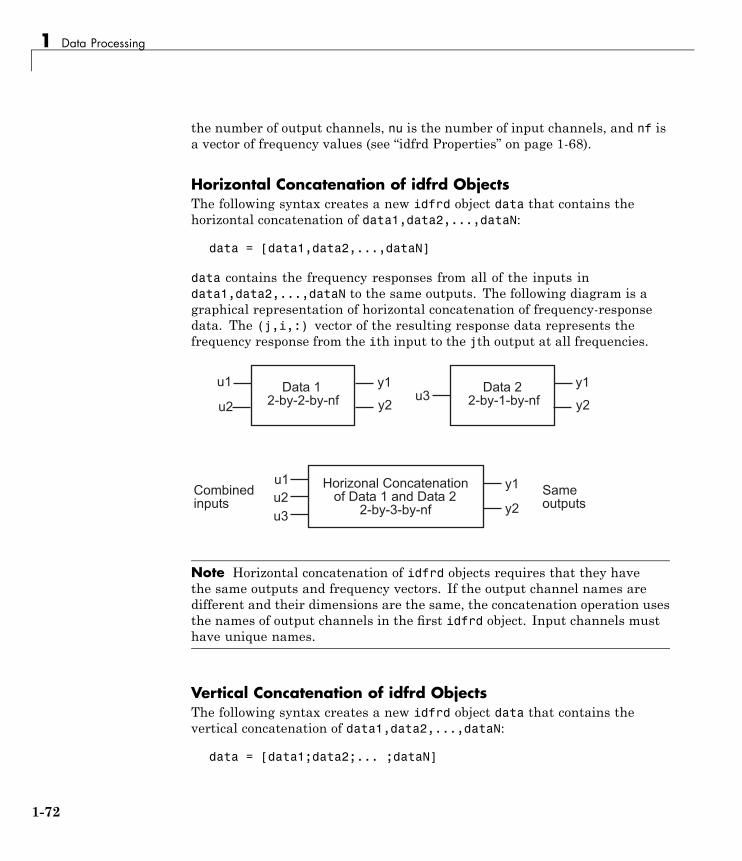
1 Data Processing
the number of output channels, nu is the number of input channels, and nf isa vector of frequency values (see “idfrd Properties” on page 1-68).
Horizontal Concatenation of idfrd ObjectsThe following syntax creates a new idfrd object data that contains thehorizontal concatenation of data1,data2,...,dataN:
data = [data1,data2,...,dataN]
data contains the frequency responses from all of the inputs indata1,data2,...,dataN to the same outputs. The following diagram is agraphical representation of horizontal concatenation of frequency-responsedata. The (j,i,:) vector of the resulting response data represents thefrequency response from the ith input to the jth output at all frequencies.
����������������������
�� ������� ������������������������������������������������!������
��
���!
�����!
��
��
��
��
��
�� "���������
������������
����������������������
Note Horizontal concatenation of idfrd objects requires that they havethe same outputs and frequency vectors. If the output channel names aredifferent and their dimensions are the same, the concatenation operation usesthe names of output channels in the first idfrd object. Input channels musthave unique names.
Vertical Concatenation of idfrd ObjectsThe following syntax creates a new idfrd object data that contains thevertical concatenation of data1,data2,...,dataN:
data = [data1;data2;... ;dataN]
1-72

Representing Frequency-Response Data Using idfrd Objects
The resulting idfrd object data contains the frequency responses fromthe same inputs in data1,data2,...,dataN to all the outputs. Thefollowing diagram is a graphical representation of vertical concatenation offrequency-response data. The (j,i,:) vector of the resulting response datarepresents the frequency response from the ith input to the jth output at allfrequencies.
�����������������������
# ����� ����������������������������������������!�����������
��
���!
��
��
��
��
����
�������������
"��������
�!
��
��
�����������������������
Note Vertical concatenation of idfrd objects requires that they have thesame inputs and frequency vectors. If the input channel names are differentand their dimensions are the same, the concatenation operation uses thenames of input channels in the first idfrd object you listed. Output channelsmust have unique names.
Concatenating Noise Spectral Data of idfrd ObjectsWhen the idfrd objects contain the frequency-response data you measuredor constructed manually, the concatenation operation combines only theResponseData properties. Because the noise spectral data does not exist(unless you also entered it manually), SpectralData is empty in both theindividual idfrd objects and the concatenated idfrd object.
However, when the idfrd objects are spectral models that you estimated, theSpectralData property is not empty and contains the power spectra andcross spectra of the output noise in the system. For each output channel, thetoolbox estimates one noise channel to explain the difference between theoutput of the model and the measured output.
1-73
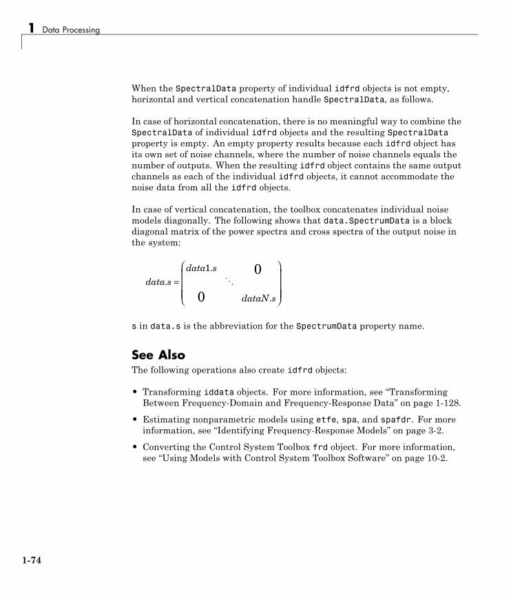
1 Data Processing
When the SpectralData property of individual idfrd objects is not empty,horizontal and vertical concatenation handle SpectralData, as follows.
In case of horizontal concatenation, there is no meaningful way to combine theSpectralData of individual idfrd objects and the resulting SpectralDataproperty is empty. An empty property results because each idfrd object hasits own set of noise channels, where the number of noise channels equals thenumber of outputs. When the resulting idfrd object contains the same outputchannels as each of the individual idfrd objects, it cannot accommodate thenoise data from all the idfrd objects.
In case of vertical concatenation, the toolbox concatenates individual noisemodels diagonally. The following shows that data.SpectrumData is a blockdiagonal matrix of the power spectra and cross spectra of the output noise inthe system:
data sdata s
dataN s
..
.
=
⎛
⎝
⎜⎜⎜⎜
⎞
⎠
⎟⎟⎟⎟
1 0
0�
s in data.s is the abbreviation for the SpectrumData property name.
See AlsoThe following operations also create idfrd objects:
• Transforming iddata objects. For more information, see “TransformingBetween Frequency-Domain and Frequency-Response Data” on page 1-128.
• Estimating nonparametric models using etfe, spa, and spafdr. For moreinformation, see “Identifying Frequency-Response Models” on page 3-2.
• Converting the Control System Toolbox frd object. For more information,see “Using Models with Control System Toolbox Software” on page 10-2.
1-74

Analyzing Data Quality Using Plots
Analyzing Data Quality Using Plots
In this section...
“Supported Data Plots” on page 1-75“Plotting Data in the System Identification Tool GUI” on page 1-75“Plotting Data at the Command Line” on page 1-81
Supported Data PlotsYou can create the following plots of your data:
• Time plot — Shows data values as a function of time.
• Spectral plot — Shows a periodogram that is computed by taking theabsolute squares of the Fourier transforms of the data, dividing by thenumber of data points, and multiplying by the sampling interval.
• Frequency-response plot — For frequency-response data, shows theamplitude and phase of the frequency-response function on a Bode plot. Fortime- and frequency-domain data, shows the empirical transfer functionestimate (see etfe) .
The plots you create using the System Identification Tool GUI provideoptions that are specific to the System Identification Toolbox product, suchas selecting specific channel pairs in a multivariate signals or convertingfrequency units between Hertz and radians per second.
The plots you create using the plot commands, such as plot, bode, and ffplot,are displayed in the standard MATLAB Figure window, which providesoptions for formatting, saving, printing, and exporting plots to a variety of fileformats. For more information, see the MATLAB Graphics documentation.
Plotting Data in the System Identification Tool GUI
• “How to Plot Data in the GUI” on page 1-76
• “Working with a Time Plot” on page 1-77
• “Working with a Data Spectra Plot” on page 1-78
1-75
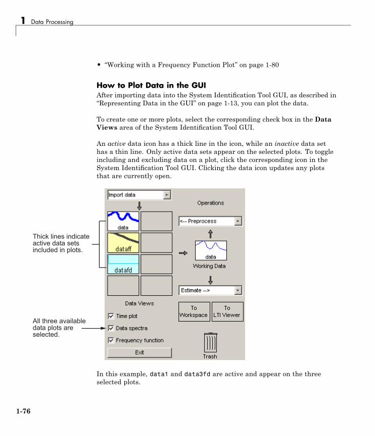
1 Data Processing
• “Working with a Frequency Function Plot” on page 1-80
How to Plot Data in the GUIAfter importing data into the System Identification Tool GUI, as described in“Representing Data in the GUI” on page 1-13, you can plot the data.
To create one or more plots, select the corresponding check box in the DataViews area of the System Identification Tool GUI.
An active data icon has a thick line in the icon, while an inactive data sethas a thin line. Only active data sets appear on the selected plots. To toggleincluding and excluding data on a plot, click the corresponding icon in theSystem Identification Tool GUI. Clicking the data icon updates any plotsthat are currently open.
���$���������������%������������������������&
'����� ��%������������������ ����&
In this example, data1 and data3fd are active and appear on the threeselected plots.
1-76
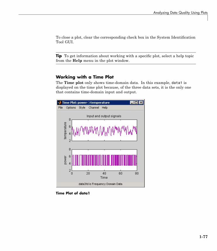
Analyzing Data Quality Using Plots
To close a plot, clear the corresponding check box in the System IdentificationTool GUI.
Tip To get information about working with a specific plot, select a help topicfrom the Help menu in the plot window.
Working with a Time PlotThe Time plot only shows time-domain data. In this example, data1 isdisplayed on the time plot because, of the three data sets, it is the only onethat contains time-domain input and output.
Time Plot of data1
1-77

1 Data Processing
Note You can plot several data sets with the same input and output channelnames. The plot displays data for all channels that have the same name. Toview a different input-output channel pair, select it from the Channel menu.For more information about selecting different input and output pairs, see“Selecting Measured and Noise Channels in Plots” on page 12-18.
The following table summarizes options that are specific to time plots, whichyou can select from the plot window menus. For general information aboutworking with System Identification Toolbox plots, see “Working with Plots inthe System Identification Tool GUI” on page 12-15.
Time Plot Options
Action Command
Toggle input display betweenpiece-wise continuous (zero-orderhold) and linear interpolation(first-order hold) between samples.
Note This option only affects thedisplay and not the intersamplebehavior specified when importingthe data.
Select Style > Staircase input forzero-order hold or Style > Regularinput for first-order hold.
Working with a Data Spectra PlotThe Data spectra plot shows a periodogram or a spectral estimate of data1and data3fd.
The periodogram is computed by taking the absolute squares of the Fouriertransforms of the data, dividing by the number of data points, and multiplyingby the sampling interval. The spectral estimate for time-domain data is asmoothed spectrum calculated using spa. For frequency-domain data, theData spectra plot shows the absolute value of the square of the actual data.
1-78

Analyzing Data Quality Using Plots
The top axes show the input and the bottom axes show the output. Thevertical axis of each plot is labeled with the corresponding channel name.
Periodograms of data1 and data3fd
Data Spectra Plot Options
Action Command
Toggle display between periodogramand spectral estimate.
Select Options > Periodogram orOptions > Spectral analysis.
Change frequency units. Select Style > Frequency (rad/s)or Style > Frequency (Hz).
Toggle frequency scale betweenlinear and logarithmic.
Select Style > Linear frequencyscale or Style > Log frequencyscale.
Toggle amplitude scale betweenlinear and logarithmic.
Select Style > Linear amplitudescale or Style > Log amplitudescale.
1-79
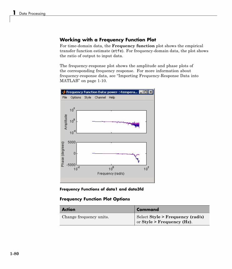
1 Data Processing
Working with a Frequency Function PlotFor time-domain data, the Frequency function plot shows the empiricaltransfer function estimate (etfe). For frequency-domain data, the plot showsthe ratio of output to input data.
The frequency-response plot shows the amplitude and phase plots ofthe corresponding frequency response. For more information aboutfrequency-response data, see “Importing Frequency-Response Data intoMATLAB” on page 1-10.
Frequency Functions of data1 and data3fd
Frequency Function Plot Options
Action Command
Change frequency units. Select Style > Frequency (rad/s)or Style > Frequency (Hz).
1-80
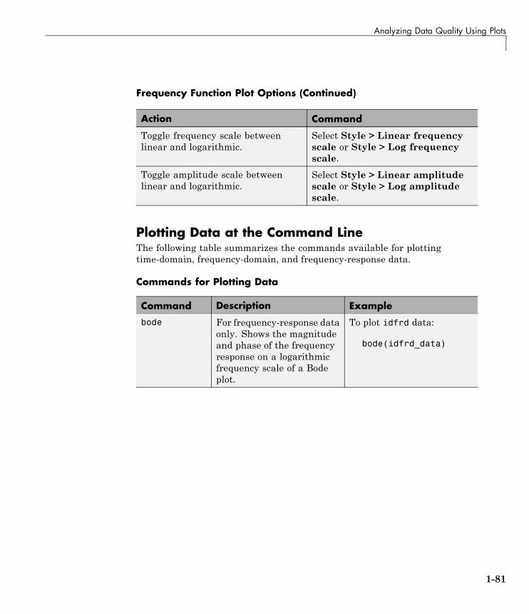
Analyzing Data Quality Using Plots
Frequency Function Plot Options (Continued)
Action Command
Toggle frequency scale betweenlinear and logarithmic.
Select Style > Linear frequencyscale or Style > Log frequencyscale.
Toggle amplitude scale betweenlinear and logarithmic.
Select Style > Linear amplitudescale or Style > Log amplitudescale.
Plotting Data at the Command LineThe following table summarizes the commands available for plottingtime-domain, frequency-domain, and frequency-response data.
Commands for Plotting Data
Command Description Example
bode For frequency-response dataonly. Shows the magnitudeand phase of the frequencyresponse on a logarithmicfrequency scale of a Bodeplot.
To plot idfrd data:
bode(idfrd_data)
1-81

1 Data Processing
Commands for Plotting Data (Continued)
Command Description Example
ffplot For frequency-responsedata only. Shows themagnitude and phase ofthe frequency response ona linear frequency scale(hertz).
To plot idfrd data:
ffplot(idfrd_data)
plot The type of plot correspondsto the type of data.For example, plottingtime-domain data generatesa time plot, and plottingfrequency-responsedata generates afrequency-response plot.
When plotting time- orfrequency-domain inputsand outputs, the top axesshow the output and thebottom axes show the input.
To plot iddata or idfrddata:
plot(data)
Note For idfrd data, thiscommand is equivalent toffplot(data).
All plot commands display the data in the standard MATLAB Figure window.For more information about working with the Figure window, see theMATLAB Graphics documentation.
To plot portions of the data, you can subreference specific samples (see“Subreferencing iddata Objects” on page 1-55 and “Subreferencing idfrdObjects” on page 1-70. For example:
plot(data(1:300))
For time-domain data, to plot only the input data as a function of time, usethe following syntax:
plot(data(:,[],:)
1-82

Analyzing Data Quality Using Plots
When data.intersample = 'zoh', the input is piece-wise constant betweensampling points on the plot. For more information about properties, see theiddata reference page.
You can generate plots of the input data in the time domain using:
plot(data.sa,data.u)
To plot frequency-domain data, you can use the following syntax:
semilogx(data.fr,abs(data.u))
In this case, sa is an abbreviation of the iddata property SamplingInstants.Similarly, fr is an abbreviation of Frequency. u is the input signal.
Note The frequencies are linearly spaced on the plot.
When you specify to plot a multivariable iddata object, each input-outputcombination is displayed one at a time in the same MATLAB Figure window.You must press Enter to update the Figure window and view the nextchannel combination. To cancel the plotting operation, press Ctrl+C.
Tip To plot specific input and output channels, use plot(data(:,ky,ku)),where ky and ku are specific output and input channel indexes or names. Formore information about subreferencing channels, see “Subreferencing DataChannels” on page 1-56.
To plot several iddata sets d1,...,dN, use plot(d1,...,dN). Input-outputchannels with the same experiment name, input name, and output nameare always plotted in the same plot.
1-83

1 Data Processing
Getting Advice About Your DataYou can use the advice command to get information about yourtime-domain or frequency-domain data. This command does not supportfrequency-response data.
Note If you are using the System Identification Tool GUI, you must exportyour data to the MATLAB workspace before you can use the advice commandon this data. For more information about exporting data, see “ExportingModels from the GUI to the MATLAB Workspace” on page 12-13.
Suppose that data is an iddata object. advice(data) displays the followinginformation about the data in the MATLAB Command Window. Ask yourselfthe following questions:
• Does it make sense to remove constant offsets and linear trends from thedata? See also detrend.
• What are the excitation levels of the signals and how does this affects themodel orders? See also pexcit.
• Is there an indication of output feedback in the data? See also feedback.When feedback is present in the system, only prediction-error methodswork well for estimating closed-loop data.
To estimate the delay from the input to the output in the system (dead time)by using the data, use the delayest command. You need to know the delaywhen specifying a model structure for estimation.
1-84

Getting Advice About Your Data
The following example shows how to get information about your data.Consider data from a single-input/single-output system sampled at 0.08 s.Use these commands to load the data and estimate the delay in the system:
load dryer2 % Load the sample input% and output data
data=iddata(y2,u2,0.08) % Create iddata objectdelayest(data) % Estimate delay (dead time)ans =
3
Use the following syntax to get advice about a data set:
advice(data) % Get advice about the data
The results of using this command suggests your identification strategy.
1-85

1 Data Processing
Selecting Subsets of Data
In this section...
“Why Select Subsets of Data?” on page 1-86“Selecting Data Using the GUI” on page 1-87“Selecting Data at the Command Line” on page 1-89
Why Select Subsets of Data?You can use data selection to create independent data sets for estimationand validation.
You can also use data selection as a way to clean the data and exclude partswith noisy or missing information. For example, when your data containsmissing values, outliers, level changes, and disturbances, you can select oneor more portions of the data that are suitable for identification and excludethe rest.
If you only have one data set and you want to estimate linear models, youshould split the data into two portions to create two independent data sets forestimation and validation, respectively. Splitting the data is selecting parts ofthe data set and saving each part independently.
You can merge several data segments into a single multiexperiment data setand identify an average model. For more information, see “Representing Datain the GUI” on page 1-13 or “Representing Time- and Frequency-Domain DataUsing iddata Objects” on page 1-47.
Note Subsets of the data set must contain enough samples to adequatelyrepresent the system, and the inputs must provide suitable excitation to thesystem.
Selecting potions of frequency-domain data is equivalent to filtering the data.For more information about filtering, see “Filtering Data” on page 1-107.
1-86

Selecting Subsets of Data
Selecting Data Using the GUI
• “Ways to Select Data in the GUI” on page 1-87
• “Selecting a Range for Time-Domain Data” on page 1-87
• “Selecting a Range of Frequency-Domain Data” on page 1-89
Ways to Select Data in the GUIYou can use System Identification Tool GUI to select ranges of data on atime-domain or frequency-domain plot. Selecting data in the frequencydomain is equivalent to passband-filtering the data.
After you select portions of the data, you can specify to use one data segmentfor estimating models and use the other data segment for validating models.For more information, see “Specifying Estimation and Validation Data” onpage 1-29.
Note Selecting <–Preprocess > Quick start performs the following actionssimultaneously:
• Remove the mean value from each channel.
• Split the data into two parts.
• Specify the first part as estimation data (orWorking Data).
• Specify the second part as Validation Data.
Selecting a Range for Time-Domain DataYou can select a range of data values on a time plot and save it as a new dataset in the System Identification Tool GUI.
Note Selecting data does not extract experiments from a data set containingmultiple experiments. For more information about multiexperiment data, see“Creating Multiexperiment Data Sets in the GUI” on page 1-33.
1-87

1 Data Processing
To extract a subset of time-domain data and save it as a new data set:
1 Import time-domain data into the System Identification Tool GUI, asdescribed in “Representing Data in the GUI” on page 1-13.
2 Drag the data set you want to subset to theWorking Data area.
3 If your data contains multiple I/O channels, in the Channel menu, selectthe channel pair you want to view. The upper plot corresponds to the inputsignal, and the lower plot corresponds to the output signal.
Although you view only one I/O channel pair at a time, your data selectionis applied to all channels in this data set.
4 Select the data of interest in either of the following ways:
• Graphically — Draw a rectangle on either the input-signal or theoutput-signal plot with the mouse to select the desired time interval.Your selection appears on both plots regardless of the plot on which youdraw the rectangle. The Time span and Samples fields are updated tomatch the selected region.
• By specifying the Time span — Edit the beginning and the end timesin seconds. The Samples field is updated to match the selected region.For example:
28.5 56.8
• By specifying the Samples range — Edit the beginning and the endindices of the sample range. The Time span field is updated to matchthe selected region. For example:
342 654
Note To clear your selection, click Revert.
5 In the Data name field, enter the name of the data set containing theselected data.
6 Click Insert. This action saves the selection as a new data set and addsit to the Data Board.
1-88

Selecting Subsets of Data
7 To select another range, repeat steps 4 to 6.
Selecting a Range of Frequency-Domain DataSelecting a range of values in frequency domain is equivalent to filteringthe data. For more information about data filtering, see “FilteringFrequency-Domain or Frequency-Response Data in the GUI” on page 1-110.
Selecting Data at the Command LineSelecting ranges of data values is equivalent to subreferencing the data.
For more information about subreferencing time-domain andfrequency-domain data, see “Subreferencing iddata Objects” on page 1-55.
For more information about subreferencing frequency-response data, see“Subreferencing idfrd Objects” on page 1-70.
1-89

1 Data Processing
Handling Missing Data and Outliers
In this section...
“Handling Missing Data” on page 1-90“Handling Outliers” on page 1-91“Example – Extracting and Modeling Specific Data Segments” on page 1-92“See Also” on page 1-93
Handling Missing DataData acquisition failures sometimes result in missing measurements both inthe input and the output signals. When you import data that contains missingvalues using the MATLAB Import Wizard, these values are automatically setto NaN (“Not-a-Number”). NaN serves as a flag for nonexistent or undefineddata. When you plot data on a time-plot that contains missing values, gapsappear on the plot where missing data exists.
You can use misdata to estimate missing values. This command linearlyinterpolates missing values to estimate the first model. Then, it uses thismodel to estimate the missing data as parameters by minimizing the outputprediction errors obtained from the reconstructed data. You can specify themodel structure you want to use in the misdata argument or estimate adefault-order model using the n4sid method. For more information, see themisdata reference page.
Note You can only use misdata on time-domain data stored in an iddataobject. For more information about creating iddata objects, see “RepresentingTime- and Frequency-Domain Data Using iddata Objects” on page 1-47.
For example, suppose y and u are output and input signals that contain NaNs.This data is sampled at 0.2 s. The following syntax creates a new iddataobject with these input and output signals.
dat = iddata(y,u,0.2) % y and u contain NaNs% representing missing data
1-90

Handling Missing Data and Outliers
Apply the misdata command to the new data object. For example:
dat1 = misdata(dat);plot(dat,dat1) % Check how the missing data
% was estimated on a time plot
Handling OutliersMalfunctions can produce errors in measured values, called outliers. Suchoutliers might be caused by signal spikes or by measurement malfunctions.If you do not remove outliers from your data, this can adversely affect theestimated models.
To identify the presence of outliers, perform one of the following tasks:
• Before estimating a model, plot the data on a time plot and identify valuesthat appear out of range.
• After estimating a model, plot the residuals and identify unusually largevalues. For more information about plotting residuals, see “Using ResidualAnalysis Plots to Validate Models” on page 8-16. Evaluate the originaldata that is responsible for large residuals. For example, for the modelModel and validation data Data, you can use the following commands toplot the residuals:
% Compute the residualsE = resid(Model,Data)
% Plot the residualsplot(E)
Next, try these techniques for removing or minimizing the effects of outliers:
• Extract the informative data portions into segments and merge them intoone multiexperiment data set (see “Example – Extracting and ModelingSpecific Data Segments” on page 1-92). For more information aboutselecting and extracting data segments, see “Selecting Subsets of Data”on page 1-86.
1-91
1 Data Processing
Tip The inputs in each of the data segments must be consistently excitingthe system. Splitting data into meaningful segments for steady-statedata results in minimum information loss. Avoid making data segmentstoo small.
• Manually replace outliers with NaNs and then use the misdata commandto reconstruct flagged data. This approach treats outliers as missing dataand is described in “Handling Missing Data” on page 1-90. Use this methodwhen your data contains several inputs and outputs, and when you havedifficulty finding reliable data segments in all variables.
• Remove outliers by prefiltering the data for high-frequency content becauseoutliers often result from abrupt changes. For more information aboutfiltering, see “Filtering Data” on page 1-107.
Note The estimation algorithm handles outliers automatically by assigninga smaller weight to outlier data. A robust error criterion applies an errorpenalty that is quadratic for small and moderate prediction errors, and islinear for large prediction errors. Because outliers produce large predictionerrors, this approach gives a smaller weight to the corresponding data pointsduring model estimation. The value LimitError (see Algorithm Properties)quantitatively distinguishes between moderate and large outliers.
Example – Extracting and Modeling Specific DataSegmentsThe following example shows how to create a multiexperiment, time-domaindata set by merging only the accurate-data segments and ignoring the rest.Modeling multiexperiment data sets produces an average model for thedifferent experiments.
You cannot simply concatenate the good data segments because the transientsat the connection points compromise the model. Instead, you must create amultiexperiment iddata object, where each experiment corresponds to a goodsegment of data, as follows:
1-92

Handling Missing Data and Outliers
% Plot the data in a MATLAB Figure windowplot(data)
% Create multiexperiment data set% by merging data segments
datam = merge(data(1:340),...data(500:897),...data(1001:1200),...data(1550:2000));
% Model the multiexperiment data set% using "experiments" 1, 2, and 4m =pem(getexp(datam,[1,2,4]))
% Validate the model by comparing its output to% the output data of experiment 3compare(getexp(datam,3),m)
See AlsoTo learn more about the theory of handling missing data and outliers, see thechapter on preprocessing data in System Identification: Theory for the User,Second Edition, by Lennart Ljung, Prentice Hall PTR, 1999.
1-93

1 Data Processing
Subtracting Trends from Signals (Detrending)
In this section...
“What Is Detrending?” on page 1-94“When to Detrend Data” on page 1-94“When Not to Detrend Data” on page 1-95“GUI and Command-Line Alternatives for Detrending Data” on page 1-96“How to Detrend Data Using the GUI” on page 1-96“How to Detrend Data at the Command Line” on page 1-97“How to Add Detrended Values to the Model Output” on page 1-98
What Is Detrending?Detrending data removes mean values or linear trends from time-series andinput/output signals. If your data set includes multiple inputs and outputs,detrending removes trends independently from each signal.
You can later restore the removed trend to simulated or predicted modeloutput, as described in “How to Add Detrended Values to the Model Output”on page 1-98.
For more information about handling drifts in the data, see the chapter onpreprocessing data in System Identification: Theory for the User, SecondEdition, by Lennart Ljung, Prentice Hall PTR, 1999.
To learn more about preparing your data for system identification, see “Waysto Process Data for System Identification” on page 1-2.
When to Detrend DataYou might want to detrend data before performing system identification, asdescribed in “Steps for Using This Toolbox”. For example, you can remove aconstant offset (zero-order trend) or drift (first-order, or linear, trend) fromyour data before modeling. Removing a trend from the data enables you tofocus your analysis on the fluctuations in the data about the trend.
1-94

Subtracting Trends from Signals (Detrending)
For linear system identification, detrending steady-state data is usefulbecause arbitrary differences between the input and output signal levelscannot be explained by a linear model.
For nonlinear black-box system identification, detrending data might behelpful when signals vary around a large signal level, you might improvecomputational accuracy by first removing the means.
When to Subtract the Mean ValuesYou can subtract mean values from your data when you have steady-state(not transient) data. If you have steady-state data, it is usually sufficientto identify linear models from signals measured relative to an equilibrium.Thus, you can avoid modeling the absolute levels in physical units.
Tip When you know the mean levels that correspond to the actual physicalequilibrium, remove the equilibrium values instead of the mean value ofthe signals for best results.
When to Subtract Linear TrendsWhen the mean levels drift during the experiment, you can eliminate this driftby removing a linear trend or several piece-wise linear trends from the signals.
Signal drift is considered a low-frequency disturbance. If you know the driftrate, you can also build a custom high-pass filter and apply it as described in“Filtering Data” on page 1-107.
When Not to Detrend DataDo not detrend your data when the physical levels are built into the underlyingmodel or when input integrators in the system require absolute signal levels.
In the case of estimating nonlinear ODE parameters (nonlinear grey-boxmodels), do not detrend the data to make sure that the models represent theactual physical levels.
1-95
1 Data Processing
When you are working with transient data (such as step or impulse response),do not remove the mean from the data. With transient data, when the outputat zero input is not zero, you might want to subtract the constant valuecorresponding to the time before the input is applied.
For nonlinear black-box models, detrending data is not always necessarybecause these models can include the trend as part of the model.
GUI and Command-Line Alternatives for DetrendingDataYou can detrend data using the System Identification Tool GUI and at thecommand line (using the detrend command).
Both the GUI and the command line let you subtract the mean values and onelinear trend from time-domain signals.
However, the detrend command provides the following additionalfunctionality not available in the GUI:
• Subtracting several linear trends connected from time-domain data atspecified breakpoints. A breakpoint is a time value that defines thediscontinuities between successive linear trends.
• Subtract a mean value from frequency-domain data.
To learn how to detrend data, see one of the following:
• “How to Detrend Data Using the GUI” on page 1-96
• “How to Detrend Data at the Command Line” on page 1-97
How to Detrend Data Using the GUIBefore you can perform this task, you must import data into the SystemIdentification Tool GUI, as described in “Importing Time-Domain Data intothe GUI” on page 1-15.
1-96

Subtracting Trends from Signals (Detrending)
Tip (For linear modeling only) Select Preprocess > Quick start to performseveral data cleaning operations, including removing the mean value fromeach signal, splitting data into two halves, specifying the first half as modelestimation data (orWorking Data), and specifying the second half as modelValidation Data.
To detrend data using the GUI:
1 In the System Identification Tool, drag the data set you want to detrend tothe Working Data rectangle.
2 Determine if you want to remove both the mean values and the lineartrend from the data.
• If yes, select Preprocess > Remove trends. This creates a new dataset in the Data Board. You are finished.
• If no, go to step 3.
3 To remove constant offsets from the data, select Preprocess > Removemeans. This selection creates a new data set in the System IdentificationTool GUI.
Note When you estimate a model from detrended data, you should alsodetrend the validation data in the same way.
How to Detrend Data at the Command LineYou can use the detrend command to perform the following operations:
• Subtract mean values from time-domain or frequency-domain data.
• Subtract one or more linear trends from time-domain data at specifiedbreakpoints, where a breakpoint is a time value that defines thediscontinuities between successive linear trends.
1-97
1 Data Processing
Before you can perform this task, you must represent your data as an iddataobject in the MATLAB workspace, as described in “Representing Time- andFrequency-Domain Data Using iddata Objects” on page 1-47.
To remove mean values from each channel in data (which is an iddataobject), use the following syntax:
data = detrend(data);
To subtract one linear trend, use the following syntax:
data = detrend(data,1);
In this case, 1 indicates that a first-order trend is removed from each signal.
Note When you estimate a model from detrended data, you should alsodetrend the validation data in the same way.
For more information about detrending options, see the detrend referencepage.
How to Add Detrended Values to the Model OutputSuppose that you estimated the model M using detrended data, where youremoved u0 and y0 from the input and output signals, respectively.
To simulate this model about nonzero equilibrium values:
1 Subtract u0 from the input signal you want to use to simulate the model.
For example, Unew=U-u0.
2 Simulate the model using the sim command and the input signal resultingfrom step 1.
For example, Ysim = sim(M,Unew,INIT), where INIT specifies the initialconditions of the simulation.
3 Add y0 to the simulated model output.
1-98

Subtracting Trends from Signals (Detrending)
For example, Ynew = Ysim+y0.
1-99

1 Data Processing
Resampling Data
In this section...
“What Is Resampling?” on page 1-100“Resampling Data Using the GUI” on page 1-101“Resampling Data at the Command Line” on page 1-101“Resampling Data Without Aliasing Effects” on page 1-103“See Also” on page 1-106
What Is Resampling?Resampling data signals in the System Identification Toolbox product appliesan antialiasing (lowpass) FIR filter to the data and changes the sampling rateof the signal by decimation or interpolation.
If your data is sampled faster than needed during the experiment, you candecimate it without information loss. If your data is sampled more slowlythan needed, there is a possibility that you miss important informationabout the dynamics at higher frequencies. Although you can resample thedata at a higher rate, the resampled values occurring between measuredsamples do not represent measured information about your system. Insteadof resampling, repeat the experiment using a higher sampling rate.
Tip You should decimate your data when it contains high-frequency noiseoutside the frequency range of the system dynamics.
Resampling takes into account how the data behaves between samples, whichyou specify when you import the data into the System Identification ToolGUI (zero-order or first-order hold). For more information about the dataproperties you specify before importing the data, see “Representing Data inthe GUI” on page 1-13.
You can resample data using the System Identification Tool GUI or theresample command. You can only resample time-domain data at uniformtime intervals.
1-100
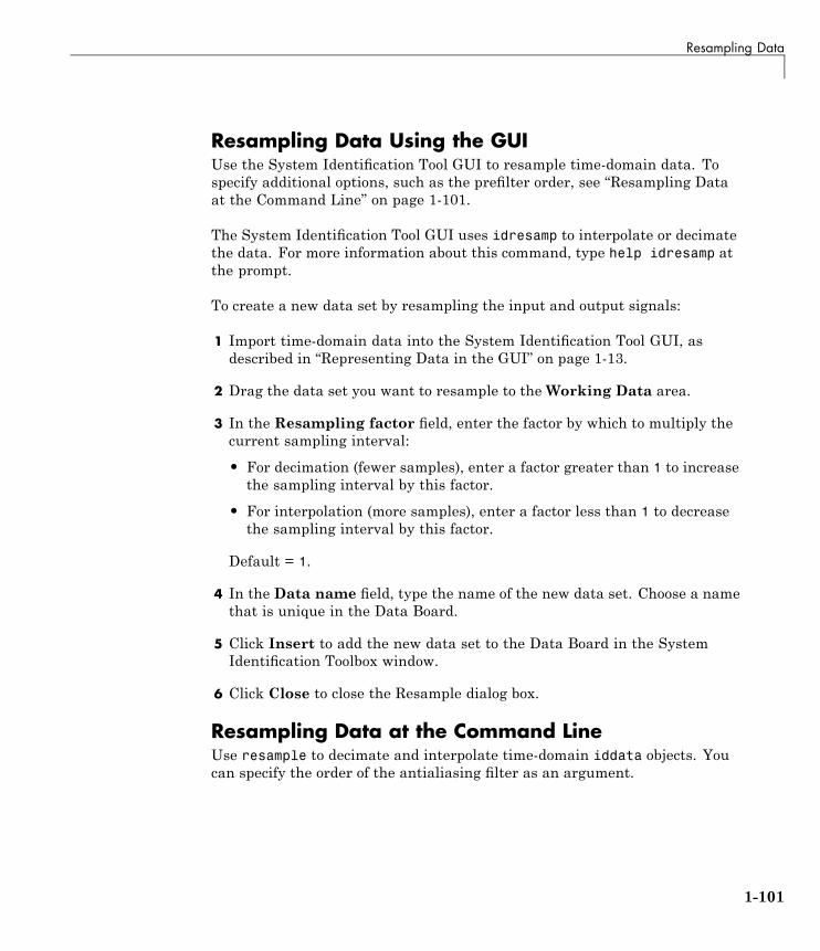
Resampling Data
Resampling Data Using the GUIUse the System Identification Tool GUI to resample time-domain data. Tospecify additional options, such as the prefilter order, see “Resampling Dataat the Command Line” on page 1-101.
The System Identification Tool GUI uses idresamp to interpolate or decimatethe data. For more information about this command, type help idresamp atthe prompt.
To create a new data set by resampling the input and output signals:
1 Import time-domain data into the System Identification Tool GUI, asdescribed in “Representing Data in the GUI” on page 1-13.
2 Drag the data set you want to resample to theWorking Data area.
3 In the Resampling factor field, enter the factor by which to multiply thecurrent sampling interval:
• For decimation (fewer samples), enter a factor greater than 1 to increasethe sampling interval by this factor.
• For interpolation (more samples), enter a factor less than 1 to decreasethe sampling interval by this factor.
Default = 1.
4 In the Data name field, type the name of the new data set. Choose a namethat is unique in the Data Board.
5 Click Insert to add the new data set to the Data Board in the SystemIdentification Toolbox window.
6 Click Close to close the Resample dialog box.
Resampling Data at the Command LineUse resample to decimate and interpolate time-domain iddata objects. Youcan specify the order of the antialiasing filter as an argument.
1-101

1 Data Processing
Note resample uses the Signal Processing Toolbox™ command, when thistoolbox is installed on your computer. If this toolbox is not installed, useidresamp instead. idresamp only lets you specify the filter order, whereasresample also lets you specify filter coefficients and the design parametersof the Kaiser window.
To create a new iddata object datar by resampling data, use the followingsyntax:
datar = resample(data,P,Q,filter_order)
In this case, P and Q are integers that specify the new sampling interval: thenew sampling interval is Q/P times the original one. You can also specify theorder of the resampling filter as a fourth argument filter_order, which isan integer (default is 10). For detailed information about resample, see thecorresponding reference page.
For example, resample(data,1,Q) results in decimation with the samplinginterval modified by a factor Q.
The next example shows how you can increase the sampling rate by a factor of1.5 and compare the signals:
plot(u)ur = resample(u,3,2);plot(u,ur)
When the Signal Processing Toolbox product is not installed, using resamplecalls idresamp instead.
idresamp uses the following syntax:
datar = idresamp(data,R,filter_order)
In this case, R=Q/P, which means that data is interpolated by a factor P andthen decimated by a factor Q. To learn more about idresamp, type helpidresamp.
1-102

Resampling Data
The data.InterSample property of the iddata object is taken into accountduring resampling (for example, first-order hold or zero-order hold). For moreinformation, see “iddata Properties” on page 1-50.
Resampling Data Without Aliasing EffectsTypically, you decimate a signal to remove the high-frequency contributionsthat result from noise from the total energy. Ideally, you want to remove theenergy contribution due to noise and preserve the energy density of the signal.
The command resample performs the decimation without aliasing effects.This command includes a factor of T to normalize the spectrum and preservethe energy density after decimation. For more information about spectrumnormalization, see “Understanding Spectrum Normalization” on page 3-11.
If you use manual decimation instead of resample—by picking every fourthsample from the signal, for example—the energy contributions from higherfrequencies are folded back into the lower frequencies. Because the totalsignal energy is preserved by this operation and this energy must now besqueezed into a smaller frequency range, the amplitude of the spectrum ateach frequency increases. Thus, the energy density of the decimated signalis not constant.
1-103
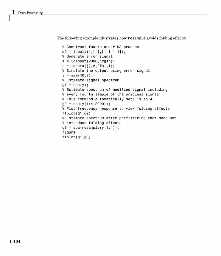
1 Data Processing
The following example illustrates how resample avoids folding effects:
% Construct fourth-order MA-processm0 = idpoly(1,[ ],[1 1 1 1]);% Generate error signale = idinput(2000,'rgs');e = iddata([],e,'Ts',1);% Simulate the output using error signaly = sim(m0,e);% Estimate signal spectrumg1 = spa(y);% Estimate spectrum of modified signal including% every fourth sample of the original signal.% This command automatically sets Ts to 4.g2 = spa(y(1:4:2000));% Plot frequency response to view folding effectsffplot(g1,g2)% Estimate spectrum after prefiltering that does not% introduce folding effectsg3 = spa(resample(y,1,4));figureffplot(g1,g3)
1-104

Resampling Data
Folding Effects with Manual Decimation
1-105

1 Data Processing
Use resample to decimate the signal before estimating the spectrum and plotthe frequency response, as follows:
g3 = spa(resample(y,1,4));figureffplot(g1,g3)
The following figure shows that the estimated spectrum of the resampledsignal has the same amplitude as the original spectrum. Thus, there is noindication of folding effects when you use resample to eliminate aliasing.
No Folding Effects When Using resample
See AlsoFor a detailed discussion about handling disturbances, see the chapter onpreprocessing data in System Identification: Theory for the User, SecondEdition, by Lennart Ljung, Prentice Hall PTR, 1999.
1-106
Filtering Data
Filtering Data
In this section...
“Supported Filters” on page 1-107“Choosing to Prefilter Your Data” on page 1-107“How to Filter Data Using the GUI” on page 1-108“How to Filter Data at the Command Line” on page 1-111“See Also” on page 1-114
Supported FiltersYou can filter the input and output signals through a linear filter beforeestimating a model in the System Identification Tool GUI or at the commandline. How you want to handle the noise in the system determines whether itis appropriate to prefilter the data.
The filter available in the System Identification Tool GUI is a fifth-order(passband) Butterworth filter. If you need to specify a custom filter, use theidfilt command.
Choosing to Prefilter Your DataPrefiltering data can help remove high-frequency noise or low-frequencydisturbances (drift). The latter application is an alternative to subtractinglinear trends from the data, as described in “Subtracting Trends from Signals(Detrending)” on page 1-94.
In addition to minimizing noise, prefiltering lets you focus your model onspecific frequency bands. The frequency range of interest often correspondsto a passband over the breakpoints on a Bode plot. For example, if you aremodeling a plant for control-design applications, you might prefilter the datato specifically enhance frequencies around the desired closed-loop bandwidth.
Prefiltering the input and output data through the same filter does not changethe input-output relationship for a linear system. However, prefiltering doeschange the noise characteristics and affects the estimated model of the system.
1-107

1 Data Processing
To get a reliable noise model, avoid prefiltering the data. Instead, setthe Focus property of the estimation algorithm to Simulation. For moreinformation about the Focus property, see the Algorithm Propertiesreference page.
Note When you prefilter during model estimation, the filtered data is used toonly model the input-to-output dynamics. However, the disturbance model iscalculated from the unfiltered data.
How to Filter Data Using the GUI
• “Filtering Time-Domain Data in the GUI” on page 1-108
• “Filtering Frequency-Domain or Frequency-Response Data in the GUI” onpage 1-110
Filtering Time-Domain Data in the GUIThe System Identification Tool GUI lets you filter time-domain data using afifth-order Butterworth filter by enhancing or selecting specific passbands.
To create a filtered data set:
1 Import time-domain data into the System Identification Tool GUI, asdescribed in “Representing Data in the GUI” on page 1-13.
2 Drag the data set you want you want to filter to theWorking Data area.
3 Select <–Preprocess > Filter. By default, this selection shows aperiodogram of the input and output spectra (see the etfe reference page).
Note To display smoothed spectral estimates instead of the periodogram,select Options > Spectral analysis. This spectral estimate is computedusing spa and your previous settings in the Spectral Model dialog box. Tochange these settings, select <–Estimate > Spectral model in the SystemIdentification Tool GUI, and specify new model settings.
1-108

Filtering Data
4 If your data contains multiple input/output channels, in the Channelmenu, select the channel pair you want to view. Although you view onlyone channel pair at a time, the filter applies to all input/output channelsin this data set.
5 Select the data of interest using one of the following ways:
• Graphically — Draw a rectangle with the mouse on either theinput-signal or the output-signal plot to select the desired frequencyinterval. Your selection is displayed on both plots regardless of the ploton which you draw the rectangle. The Range field is updated to matchthe selected region. If you need to clear your selection, right-click theplot.
• Specify the Range— Edit the beginning and the end frequency values.
For example:
8.5 20.0 (rad/s).
Tip To change the frequency units from rad/s to Hz, selectStyle > Frequency (Hz). To change the frequency units from Hz torad/s, select Style > Frequency (rad/s).
6 In the Range is list, select one of the following:
• Pass band— Allows data in the selected frequency range.
• Stop band— Excludes data in the selected frequency range.
7 Click Filter to preview the filtered results. If you are satisfied, go to step 8.Otherwise, return to step 5.
8 In the Data name field, enter the name of the data set containing theselected data.
9 Click Insert to save the selection as a new data set and add it to the DataBoard.
10 To select another range, repeat steps 5 to 9.
1-109
1 Data Processing
Filtering Frequency-Domain or Frequency-Response Data inthe GUIFor frequency-domain and frequency-response data, filtering is equivalent toselecting specific data ranges.
To select a range of data in frequency-domain or frequency-response data:
1 Import data into the System Identification Tool GUI, as described in“Representing Data in the GUI” on page 1-13.
2 Drag the data set you want you want to filter to theWorking Data area.
3 Select <–Preprocess > Select range. This selection displays one of thefollowing plots:
• Frequency-domain data — Plot shows the absolute of the squares of theinput and output spectra.
• Frequency-response data — Top axes show the frequency responsemagnitude equivalent to the ratio of the output to the input, and thebottom axes show the ratio of the input signal to itself, which has thevalue of 1 at all frequencies.
4 If your data contains multiple input/output channels, in the Channelmenu, select the channel pair you want to view. Although you view onlyone channel pair at a time, the filter applies to all input/output channelsin this data set.
5 Select the data of interest using one of the following ways:
• Graphically — Draw a rectangle with the mouse on either theinput-signal or the output-signal plot to select the desired frequencyinterval. Your selection is displayed on both plots regardless of the ploton which you draw the rectangle. The Range field is updated to matchthe selected region.
If you need to clear your selection, right-click the plot.
• Specify the Range— Edit the beginning and the end frequency values.
For example:
8.5 20.0 (rad/s).
1-110
Filtering Data
Tip If you need to change the frequency units from rad/s to Hz, selectStyle > Frequency (Hz). To change the frequency units from Hz torad/s, select Style > Frequency (rad/s).
6 In the Range is list, select one of the following:
• Pass band— Allows data in the selected frequency range.
• Stop band— Excludes data in the selected frequency range.
7 In the Data name field, enter the name of the data set containing theselected data.
8 Click Insert. This action saves the selection as a new data set and addsit to the Data Board.
9 To select another range, repeat steps 5 to 8.
How to Filter Data at the Command Line
• “Simple Passband Filter” on page 1-111
• “Defining a Custom Filter” on page 1-112
• “Causal and Noncausal Filters” on page 1-113
Simple Passband FilterUse idfilt to apply passband and other custom filters to a time-domain ora frequency-domain iddata object.
In general, you can specify any custom filter. Use this syntax to filter aniddata object data using the filter called filter:
fdata = idfilt(data,filter)
In the simplest case, you can specify a passband filter for time-domain datausing the following syntax:
fdata = idfilt(data,[wl wh])
1-111
1 Data Processing
In this case, w1 and wh represent the low and high frequencies of the passband,respectively.
You can specify several passbands, as follows:
filter=[[w1l,w1h];[ w2l,w2h]; ....;[wnl,wnh]]
The filter is an n-by-2 matrix, where each row defines a passband in radiansper second.
To define a stopband between ws1 and ws2, use
filter = [0 ws1; ws2 Nyqf]
where, Nyqf is the Nyquist frequency.
For time-domain data, the passband filtering is cascaded Butterworth filters ofspecified order. The default filter order is 5. The Butterworth filter is the sameas butter in the Signal Processing Toolbox product. For frequency-domaindata, select the indicated portions of the data to perform passband filtering.
Defining a Custom FilterUse idfilt to apply passband and other custom filters to a time-domain ora frequency-domain iddata object.
In general, you can specify any custom filter. Use this syntax to filter aniddata object data using the filter called filter:
fdata = idfilt(data,filter)
You can define a general single-input/single-output (SISO) system for filteringtime-domain or frequency-domain data. For frequency-domain only, you canspecify the (nonparametric) frequency response of the filter.
You use this syntax to filter an iddata object data using a custom filterspecified by filter:
fdata = idfilt(data,filter)
filter can be also any of the following:
1-112

Filtering Data
filter = idmfilter = {num,den}filter = {A,B,C,D}
idm is a SISO idmodel or LTI object. For more information about LTI objects,see the Control System Toolbox documentation.
{num,den} defines the filter as a transfer function as a cell array of numeratorand denominator filter coefficients.
{A,B,C,D} is a cell array of SISO state-space matrices.
Specifically for frequency-domain data, you specify the frequency responseof the filter:
filter = Wf
Here, Wf is a vector of real or complex values that define the filterfrequency response, where the inputs and outputs of data at frequencydata.Frequency(kf) are multiplied by Wf(kf). Wf is a column vector withthe length equal to the number of frequencies in data.
When data contains several experiments, Wf is a cell array with the lengthequal to the number of experiments in data.
Causal and Noncausal FiltersFor time-domain data, the filtering is causal by default. Causal filterstypically introduce a phase shift in the results. To use a noncausal zero-phasefilter (corresponding to filtfilt in the Signal Processing Toolbox product),specify a third argument in idfilt:
fdata = idfilt(data,filter,'noncausal')
For frequency-domain data, the signals are multiplied by the frequencyresponse of the filter. With the filters defined as passband filters, thiscalculation gives ideal, zero-phase filtering (“brick wall filters”). Frequenciesthat have been assigned zero weight by the filter (outside the passband orvia frequency response) are removed.
1-113
1 Data Processing
When you apply idfilt to an idfrd data object, the data is first convertedto a frequency-domain iddata object (see “Transforming BetweenFrequency-Domain and Frequency-Response Data” on page 1-128). The resultis an iddata object.
See AlsoTo learn how to filter data during linear model estimation instead, you canset the Focus property of the estimation algorithm to Filter and specify thefilter characteristics. For more information about model properties, see theAlgorithm Properties reference page.
For more information about prefiltering data, see the chapter on preprocessingdata in System Identification: Theory for the User, Second Edition, by LennartLjung, Prentice Hall PTR, 1999.
For practical examples of prefiltering data, see the section on posttreatmentof data in Modeling of Dynamic Systems, by Lennart Ljung and Torkel Glad,Prentice Hall PTR, 1994.
1-114

Generating Data Using Simulation
Generating Data Using Simulation
In this section...
“Commands for Generating and Simulating Data” on page 1-115“Example – Creating Data with Periodic Inputs” on page 1-116“Example – Generating Data Using Simulation” on page 1-117“Simulating Data Using Other MathWorks Products” on page 1-118
Commands for Generating and Simulating DataYou can generate input data and simulate output data using a specifiedmodel structure.
Simulating output data requires that you have a parametric model. For moreinformation about commands for constructing models, see “Commands forConstructing Model Structures” on page 2-13.
To generate input data, use idinput to construct a signal with the desiredcharacteristics, such as a random Gaussian or binary signal or a sinusoid.idinput returns a matrix of input values.
The following table lists the commands you can use to simulate output data.For more information about these commands, see the corresponding referencepages.
Commands for Generating and Simulating Data
Command Description Example
iddata Constructs an iddataobject with inputchannels only.
To construct input data data, use thefollowing command:
data = iddata([ ],[u v])
u is the input data, and v is white noise.
1-115

1 Data Processing
Commands for Generating and Simulating Data (Continued)
Command Description Example
idinput Constructs a signalwith the desiredcharacteristics, suchas a random Gaussianor binary signal or asinusoid, and returns amatrix of input values.
u = iddata([],...idinput(400,'rbs',[0 0.3]));
sim Simulates response databased on existing linearor nonlinear parametricmodel in the MATLABworkspace.
To simulate the model output y for a giveninput, use the following command:
y = sim(m,data)
m is the model object name, and data is inputdata matrix or iddata object.
Example – Creating Data with Periodic Inputs
1 Create a periodic input for two inputs and consisting of five periods, whereeach period is 300 samples.
per_u = idinput([300 2 5])
2 Create an iddata object using the periodic input and leaving the outputempty.
u = iddata([],per_u,'Period',...[300; 300]);
You can use the periodic input to simulate the output, and the use etfe tocompute the estimated response of the model.
% Construct polynomial modelm0 =idpoly([1 -1.5 0.7],[0 1 0.5]);% Construct random binary inputu = idinput([10 1 150],'rbs');
1-116
Generating Data Using Simulation
% Construct input data and noiseu = iddata([],u,'Period',10);e = iddata([],randn(1500,1));% Simulate model output with noisey = sim(m0,[u e])% Estimate frequency responseg = etfe([y u])% Generate Bode plotbode(g,'x',m0)
For periodic input, etfe honors the period and computes the frequencyresponse using an appropriate frequency grid. In this case, the Bode plotshows a good fit at the five excited frequencies.
Example – Generating Data Using SimulationThis example demonstrates how you can create input data and a model, andthen use the data and the model to simulate output data. You create theARMAX model and simulate output data with random binary input u.
1 Load the three-input and one-output sample data.
load iddata8
2 Construct an ARMAX model, using the following commands:
A = [1 -1.2 0.7];B(1,:) = [0 1 0.5 0.1]; % first inputB(2,:) = [0 1.5 -0.5 0]; % second inputB(3,:) = [0 -0.1 0.5 -0.1]; % third inputC = [1 0 0 0 0];Ts = 1;m = idpoly(A,B,C,'Ts',1);
In this example, the leading zeros in the B matrix indicate the input delay(nk), which is 1 for each input channel. The trailing zero in B(2,:) makesthe number of coefficients equal for all channels.
3 Construct pseudorandom binary data for input to the simulation.
u = idinput([200,3],'prbs');
1-117
1 Data Processing
4 Simulate the model output.
sim(m,u)
5 Compare model output to measured data to see how well the modelscaptures the underlying dynamics.
compare(z8,m)
Simulating Data Using Other MathWorks ProductsYou can also simulate data using the Simulink® and Signal ProcessingToolbox software. Data simulated outside the System Identification Toolboxproduct must be in the MATLAB workspace. For more information aboutsimulating models using the Simulink software, see “Simulating ModelOutput” on page 11-6.
1-118
Transforming Between Time- and Frequency-Domain Data
Transforming Between Time- and Frequency-Domain Data
In this section...
“Transforming Data Domain in the GUI” on page 1-119“Transforming Data Domain at the Command Line” on page 1-126
Transforming Data Domain in the GUI
• “Transforming Time-Domain Data” on page 1-119
• “Transforming Frequency-Domain Data” on page 1-123
• “Transforming Frequency-Response Data” on page 1-124
• “See Also” on page 1-126
Transforming Time-Domain DataIn the System Identification Tool GUI, time-domain data has an icon with awhite background. You can transform time-domain data to frequency-domainor frequency-response data. The frequency values of the resulting frequency
vector range from 0 to the Nyquist frequency fS Ts= π , where Ts is thesampling interval.
Transforming from time-domain to frequency-response data is equivalent toestimating a model from the data using the spafdr method.
1-119
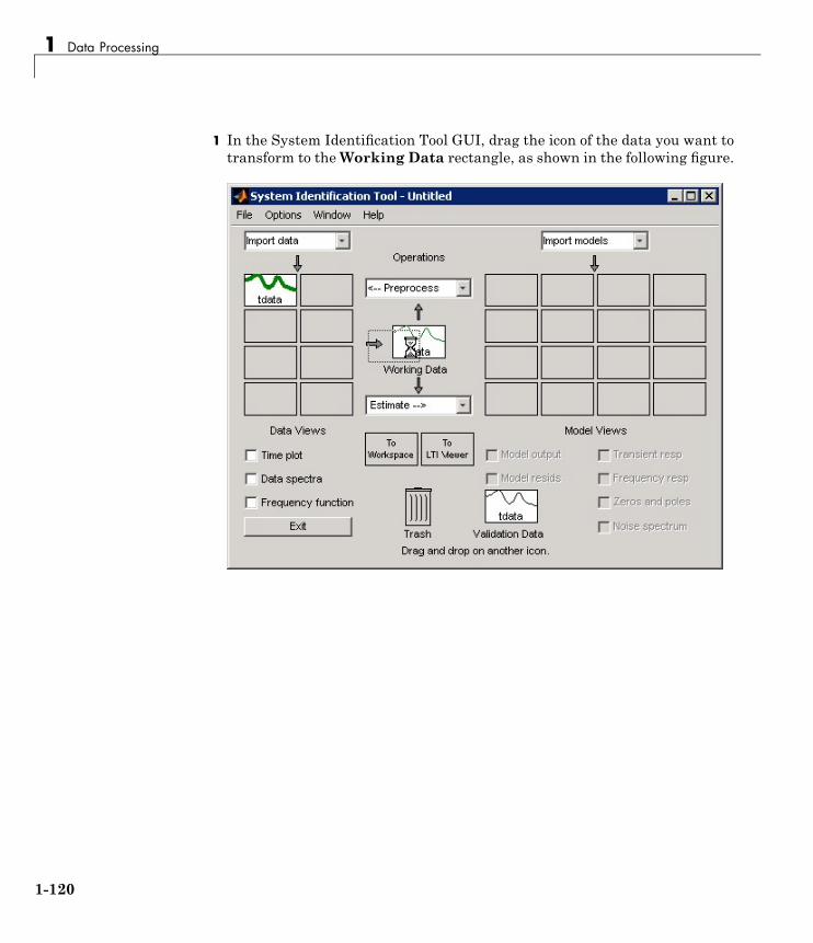
1 Data Processing
1 In the System Identification Tool GUI, drag the icon of the data you want totransform to theWorking Data rectangle, as shown in the following figure.
1-120

Transforming Between Time- and Frequency-Domain Data
2 In the Operations area, select <–Preprocess > Transform data in thedrop-down menu to open the Transform Data dialog box.
1-121
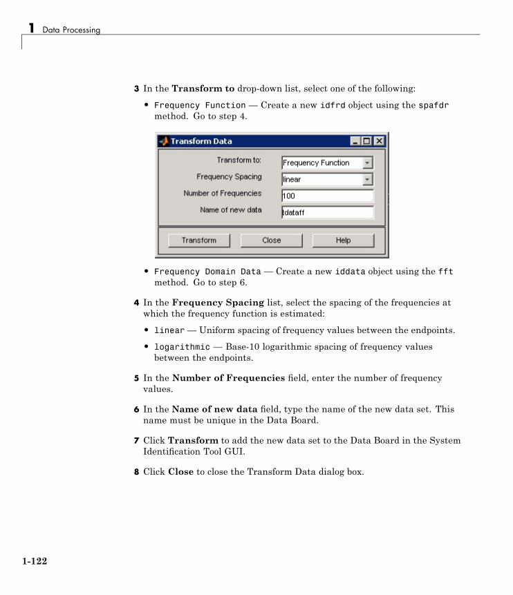
1 Data Processing
3 In the Transform to drop-down list, select one of the following:
• Frequency Function — Create a new idfrd object using the spafdrmethod. Go to step 4.
• Frequency Domain Data— Create a new iddata object using the fftmethod. Go to step 6.
4 In the Frequency Spacing list, select the spacing of the frequencies atwhich the frequency function is estimated:
• linear— Uniform spacing of frequency values between the endpoints.
• logarithmic — Base-10 logarithmic spacing of frequency valuesbetween the endpoints.
5 In the Number of Frequencies field, enter the number of frequencyvalues.
6 In the Name of new data field, type the name of the new data set. Thisname must be unique in the Data Board.
7 Click Transform to add the new data set to the Data Board in the SystemIdentification Tool GUI.
8 Click Close to close the Transform Data dialog box.
1-122

Transforming Between Time- and Frequency-Domain Data
Transforming Frequency-Domain DataIn the System Identification Tool GUI, frequency-domain data has an iconwith a green background. You can transform frequency-domain data totime-domain or frequency-response (frequency-function) data.
Transforming from time-domain or frequency-domain data tofrequency-response data is equivalent to estimating a nonparametric model ofthe data using the spafdr method.
1 In the System Identification Tool GUI, drag the icon of the data you wantto transform to the Working Data rectangle.
2 Select <–Preprocess > Transform data.
3 In the Transform to list, select one of the following:
• Frequency Function — Create a new idfrd object using the spafdrmethod. Go to step 4.
• Time Domain Data — Create a new iddata object using the ifft(inverse fast Fourier transform) method. Go to step 6.
4 In the Frequency Spacing list, select the spacing of the frequencies atwhich the frequency function is estimated:
• linear— Uniform spacing of frequency values between the endpoints.
• logarithmic — Base-10 logarithmic spacing of frequency valuesbetween the endpoints.
5 In the Number of Frequencies field, enter the number of frequencyvalues.
6 In the Name of new data field, type the name of the new data set. Thisname must be unique in the Data Board.
7 Click Transform to add the new data set to the Data Board in the SystemIdentification Tool GUI.
8 Click Close to close the Transform Data dialog box.
1-123
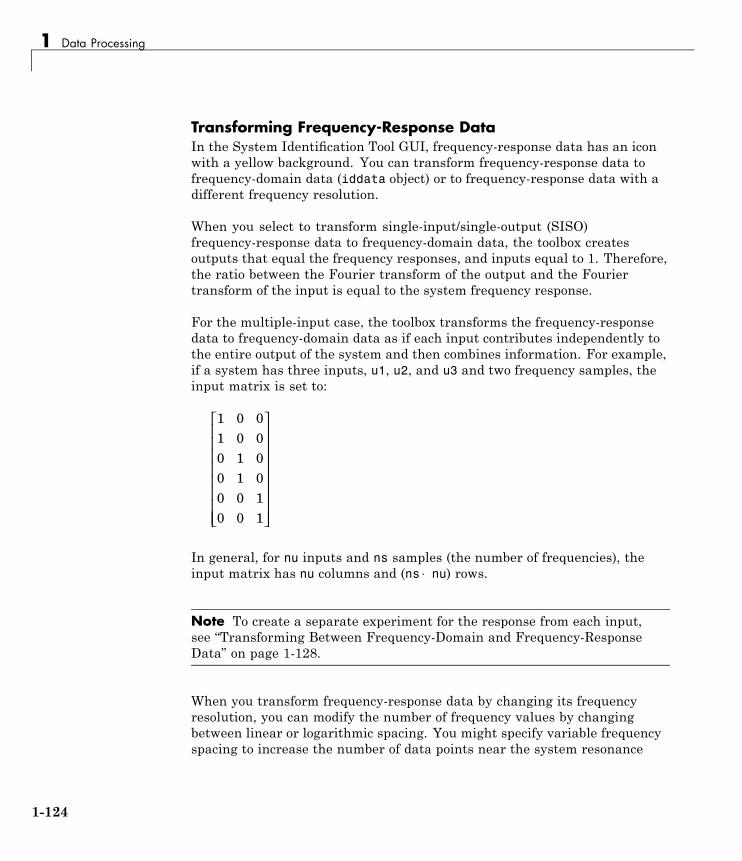
1 Data Processing
Transforming Frequency-Response DataIn the System Identification Tool GUI, frequency-response data has an iconwith a yellow background. You can transform frequency-response data tofrequency-domain data (iddata object) or to frequency-response data with adifferent frequency resolution.
When you select to transform single-input/single-output (SISO)frequency-response data to frequency-domain data, the toolbox createsoutputs that equal the frequency responses, and inputs equal to 1. Therefore,the ratio between the Fourier transform of the output and the Fouriertransform of the input is equal to the system frequency response.
For the multiple-input case, the toolbox transforms the frequency-responsedata to frequency-domain data as if each input contributes independently tothe entire output of the system and then combines information. For example,if a system has three inputs, u1, u2, and u3 and two frequency samples, theinput matrix is set to:
1 0 01 0 00 1 00 1 00 0 10 0 1
⎡
⎣
⎢⎢⎢⎢⎢⎢⎢⎢
⎤
⎦
⎥⎥⎥⎥⎥⎥⎥⎥
In general, for nu inputs and ns samples (the number of frequencies), theinput matrix has nu columns and (ns ⋅ nu) rows.
Note To create a separate experiment for the response from each input,see “Transforming Between Frequency-Domain and Frequency-ResponseData” on page 1-128.
When you transform frequency-response data by changing its frequencyresolution, you can modify the number of frequency values by changingbetween linear or logarithmic spacing. You might specify variable frequencyspacing to increase the number of data points near the system resonance
1-124

Transforming Between Time- and Frequency-Domain Data
frequencies, and also make the frequency vector coarser in the region outsidethe system dynamics. Typically, high-frequency noise dominates awayfrom frequencies where interesting system dynamics occur. The SystemIdentification Tool GUI lets you specify logarithmic frequency spacing, whichresults in a variable frequency resolution.
Note The spafdr command lets you lets you specify any variable frequencyresolution.
1 In the System Identification Tool GUI, drag the icon of the data you wantto transform to the Working Data rectangle.
2 Select <–Preprocess > Transform data.
3 In the Transform to list, select one of the following:
• Frequency Domain Data— Create a new iddata object. Go to step 6.
• Frequency Function — Create a new idfrd object with differentresolution (number and spacing of frequencies) using the spafdrmethod.Go to step 4.
4 In the Frequency Spacing list, select the spacing of the frequencies atwhich the frequency function is estimated:
• linear— Uniform spacing of frequency values between the endpoints.
• logarithmic — Base-10 logarithmic spacing of frequency valuesbetween the endpoints.
5 In the Number of Frequencies field, enter the number of frequencyvalues.
6 In the Name of new data field, type the name of the new data set. Thisname must be unique in the Data Board.
7 Click Transform to add the new data set to the Data Board in the SystemIdentification Tool GUI.
8 Click Close to close the Transform Data dialog box.
1-125

1 Data Processing
See AlsoFor a description of time-domain, frequency-domain, and frequency-responsedata, see “Importing Data into the MATLAB Workspace” on page 1-5.
To learn how to transform data at the command line instead of the GUI, see“Transforming Data Domain at the Command Line” on page 1-126.
Transforming Data Domain at the Command Line
• “Supported Data Transformations” on page 1-126
• “Transforming Between Time and Frequency Domain” on page 1-127
• “Transforming Between Frequency-Domain and Frequency-ResponseData” on page 1-128
• “See Also” on page 1-130
Supported Data TransformationsThe following table shows the different ways you can transform data from onedata domain to another. If the transformation is supported for a given rowand column combination in the table, the method used by the software islisted in the cell at their intersection.
Original DataFormat
To Time Domain(iddata object)
To FrequencyDomain(iddata object)
To FrequencyFunction(idfrd object)
Time Domain(iddata object)
No. Yes, using fft. Yes, using etfe,spa, or spafdr.
1-126

Transforming Between Time- and Frequency-Domain Data
Original DataFormat
To Time Domain(iddata object)
To FrequencyDomain(iddata object)
To FrequencyFunction(idfrd object)
FrequencyDomain(iddata object)
Yes, using ifft. No. Yes, using etfe,spa, or spafdr.
FrequencyFunction(idfrd object)
No. Yes. Calculationcreatesfrequency-domainiddata objectthat has thesame ratiobetween outputand input as theoriginal idfrdobject.
Yes. Calculatesa frequencyfunction withdifferentresolution(number andspacing offrequencies)using spafdr.
Transforming Between Time and Frequency DomainThe iddata object stores time-domain or frequency-domain data. Thefollowing table summarizes the commands for transforming data betweentime and frequency domains.
1-127
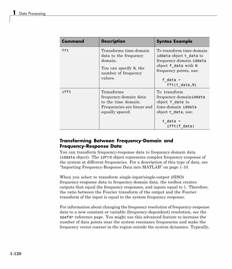
1 Data Processing
Command Description Syntax Example
fft Transforms time-domaindata to the frequencydomain.
You can specify N, thenumber of frequencyvalues.
To transform time-domainiddata object t_data tofrequency-domain iddataobject f_data with Nfrequency points, use:
f_data =fft(t_data,N)
ifft Transformsfrequency-domain datato the time domain.Frequencies are linear andequally spaced.
To transformfrequency-domainiddataobject f_data totime-domain iddataobject t_data, use:
t_data =ifft(f_data)
Transforming Between Frequency-Domain andFrequency-Response DataYou can transform frequency-response data to frequency-domain data(iddata object). The idfrd object represents complex frequency-response ofthe system at different frequencies. For a description of this type of data, see“Importing Frequency-Response Data into MATLAB” on page 1-10.
When you select to transform single-input/single-output (SISO)frequency-response data to frequency-domain data, the toolbox createsoutputs that equal the frequency responses, and inputs equal to 1. Therefore,the ratio between the Fourier transform of the output and the Fouriertransform of the input is equal to the system frequency response.
For information about changing the frequency resolution of frequency-responsedata to a new constant or variable (frequency-dependent) resolution, see thespafdr reference page. You might use this advanced feature to increase thenumber of data points near the system resonance frequencies and make thefrequency vector coarser in the region outside the system dynamics. Typically,
1-128

Transforming Between Time- and Frequency-Domain Data
high-frequency noise dominates away from frequencies where interestingsystem dynamics occur.
Note You cannot transform an idfrd object to a time-domain iddata object.
To transform an idfrd object with the name idfrdobj to a frequency-domainiddata object, use the following syntax:
dataf = iddata(idfrdobj)
The resulting frequency-domain iddata object contains values at the samefrequencies as the original idfrd object.
For the multiple-input case, the toolbox represents frequency-response dataas if each input contributes independently to the entire output of the systemand then combines information. For example, if a system has three inputs,u1, u2, and u3 and two frequency samples, the input matrix is set to:
1 0 01 0 00 1 00 1 00 0 10 0 1
⎡
⎣
⎢⎢⎢⎢⎢⎢⎢⎢
⎤
⎦
⎥⎥⎥⎥⎥⎥⎥⎥
In general, for nu inputs and ns samples, the input matrix has nu columnsand (ns ⋅ nu) rows.
If you have ny outputs, the transformation operation produces an outputmatrix has ny columns and (ns ⋅ nu) rows using the values in the complexfrequency response G(iw) matrix (ny-by-nu-by-ns). In this example, y1 isdetermined by unfolding G(1,1,:), G(1,2,:), and G(1,3,:) into threecolumn vectors and vertically concatenating these vectors into a single column.Similarly, y2 is determined by unfolding G(2,1,:), G(2,2,:), and G(2,3,:)into three column vectors and vertically concatenating these vectors.
1-129

1 Data Processing
If you are working with multiple inputs, you also have the option ofstoring the contribution by each input as an independent experiment in amultiexperiment data set. To transform an idfrd object with the nameidfrdobj to a multiexperiment data set datf, where each experimentcorresponds to each of the inputs in idfrdobj
datf = iddata(idfrdobj,'me')
In this example, the additional argument 'me' specifies that multipleexperiments are created.
By default, transformation from frequency-response to frequency-domaindata strips away frequencies where the response is inf or NaN. To preservethe entire frequency vector, use datf = iddata(idfrdobj,'inf'). For moreinformation, type help idfrd/iddata.
See AlsoTransforming from time-domain or frequency-domain data tofrequency-response data is equivalent to creating a frequency-response modelfrom the data. For more information, see “Identifying Frequency-ResponseModels” on page 3-2.
1-130

Manipulating Complex-Valued Data
Manipulating Complex-Valued Data
In this section...
“Supported Operations for Complex Data” on page 1-131“Processing Complex iddata Signals at the Command Line” on page 1-131
Supported Operations for Complex DataSystem Identification Toolbox estimation algorithms support complex data.For example, the following estimation commands estimate complex modelsfrom complex data: ar, armax, arx, bj, covf, ivar, iv4, oe, pem, spa, andn4sid.
Model transformation routines, such as freqresp and zpkdata, work forcomplex-valued models. However, they do not provide pole-zero confidenceregions. For complex models, the parameter variance-covariance informationrefers to the complex-valued parameters and the accuracy of the real andimaginary is not computed separately.
The display commands compare and plot also work with complex-valueddata and models, but only show the absolute values of the signals. To plotthe real and imaginary parts of the data separately, use plot(real(data))and plot(imag(data)), respectively.
Processing Complex iddata Signals at the CommandLineIf the iddata object data contains complex values, you can use the followingcommands to process the complex data and create a new iddata object.
Command Description
abs(data) Absolute value of complex signals in iddata object.angle(data) Phase angle (in radians) of each complex signals in
iddata object.
1-131

1 Data Processing
Command Description
complex(data) For time-domain data, this command makes the iddataobject complex—even when the imaginary parts arezero. For frequency-domain data that only storesthe values for nonnegative frequencies, such thatrealdata(data)=1, it adds signal values for negativefrequencies using complex conjugation.
imag(data) Selects the imaginary parts of each signal in iddataobject.
isreal(data) 1 when data (time-domain or frequency-domain)contains only real input and output signals, and returns0 when data (time-domain or frequency-domain)contains complex signals.
real(data) Real part of complex signals in iddata object.realdata(data) Returns a value of 1 when data is a real-valued,
time-domain signal, and returns 0 otherwise.
For example, suppose that you create a frequency-domain iddata object Datfby applying fft to a real-valued time-domain signal to take the Fouriertransform of the signal. The following is true for Datf:
isreal(Datf) = 0realdata(Datf) = 1
1-132

2
Choosing Your SystemIdentification Strategy
• “Recommended Model Estimation Sequence” on page 2-2
• “Supported Models for Time- and Frequency-Domain Data” on page 2-4
• “Supported Continuous-Time and Discrete-Time Models” on page 2-7
• “Commands for Model Estimation” on page 2-9
• “Creating Model Structures at the Command Line” on page 2-11
• “Modeling Multiple-Output Systems” on page 2-21

2 Choosing Your System Identification Strategy
Recommended Model Estimation SequenceSystem identification is an iterative process, where you identify modelswith different structures from data and compare model performance. Youstart by estimating the parameters of simple model structures. If the modelperformance is poor, you gradually increase the complexity of the modelstructure. Ultimately, you choose the simplest model that best describesthe dynamics of your system.
Another reason to start with simple model structures is that higher-ordermodels are not always more accurate. Increasing model complexity increasesthe uncertainties in parameter estimates and typically requires more data(which is common in the case of nonlinear models).
Note Model structure is not the only factor that determines model accuracy.If your model is poor, you might need to preprocess your data by removingoutliers or filtering noise. For more information, see “Ways to Process Datafor System Identification” on page 1-2.
Estimate impulse-response and frequency-response models first to gaininsight into the system dynamics and assess whether a linear model issufficient. Then, estimate parametric models in the following order:
1 ARX polynomial and state-space models provide the simplest structures.These models let you estimate the model order and noise dynamics.
In the System Identification Tool GUI. Select to estimate the ARXlinear parametric model and the state-space model using the N4SIDmethod.
At the command line. Use the arx and the n4sid commands.
For more information, see “Identifying Input-Output Polynomial Models”on page 3-41 and “Identifying State-Space Models” on page 3-73.
2 ARMAX and BJ polynomial models provide more complex structures andrequire iterative estimation. Try several model orders and keep the modelorders as low as possible.
2-2

Recommended Model Estimation Sequence
In the System Identification Tool GUI. Select to estimate the BJ andARMAX linear parametric models.
At the command line. Use the bj or armax commands.
For more information, see “Identifying Input-Output Polynomial Models”on page 3-41.
3 Nonlinear ARX or Hammerstein-Wiener models provide nonlinearstructures. For more information, see Chapter 4, “Nonlinear Black-BoxModel Identification”.
For general information about choosing you model strategy, see “ChoosingWhich Models to Estimate”. For information about validating models, see“Overview of Model Validation and Plots” on page 8-2.
To learn more about refining estimated models, see “Refining LinearParametric Models” on page 3-103 and “Refining Nonlinear Black-BoxModels” on page 4-28.
2-3
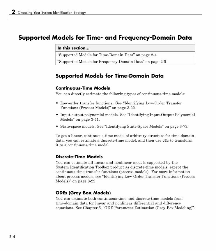
2 Choosing Your System Identification Strategy
Supported Models for Time- and Frequency-Domain Data
In this section...
“Supported Models for Time-Domain Data” on page 2-4“Supported Models for Frequency-Domain Data” on page 2-5
Supported Models for Time-Domain Data
Continuous-Time ModelsYou can directly estimate the following types of continuous-time models:
• Low-order transfer functions. See “Identifying Low-Order TransferFunctions (Process Models)” on page 3-22.
• Input-output polynomial models. See “Identifying Input-Output PolynomialModels” on page 3-41.
• State-space models. See “Identifying State-Space Models” on page 3-73.
To get a linear, continuous-time model of arbitrary structure for time-domaindata, you can estimate a discrete-time model, and then use d2c to transformit to a continuous-time model.
Discrete-Time ModelsYou can estimate all linear and nonlinear models supported by theSystem Identification Toolbox product as discrete-time models, except thecontinuous-time transfer functions (process models). For more informationabout process models, see “Identifying Low-Order Transfer Functions (ProcessModels)” on page 3-22.
ODEs (Grey-Box Models)You can estimate both continuous-time and discrete-time models fromtime-domain data for linear and nonlinear differential and differenceequations. See Chapter 5, “ODE Parameter Estimation (Grey-Box Modeling)”.
2-4
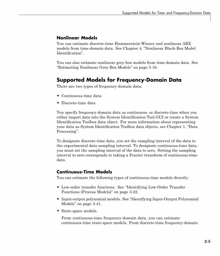
Supported Models for Time- and Frequency-Domain Data
Nonlinear ModelsYou can estimate discrete-time Hammerstein-Wiener and nonlinear ARXmodels from time-domain data. See Chapter 4, “Nonlinear Black-Box ModelIdentification”.
You can also estimate nonlinear grey-box models from time-domain data. See“Estimating Nonlinear Grey-Box Models” on page 5-16.
Supported Models for Frequency-Domain DataThere are two types of frequency-domain data:
• Continuous-time data
• Discrete-time data
You specify frequency-domain data as continuous- or discrete-time when youeither import data into the System Identification Tool GUI or create a SystemIdentification Toolbox data object. For more information about representingyour data as System Identification Toolbox data objects, see Chapter 1, “DataProcessing”.
To designate discrete-time data, you set the sampling interval of the data tothe experimental data sampling interval. To designate continuous-time data,you must set the sampling interval of the data to zero. Setting the samplinginterval to zero corresponds to taking a Fourier transform of continuous-timedata.
Continuous-Time ModelsYou can estimate the following types of continuous-time models directly:
• Low-order transfer functions. See “Identifying Low-Order TransferFunctions (Process Models)” on page 3-22.
• Input-output polynomial models. See “Identifying Input-Output PolynomialModels” on page 3-41.
• State-space models.
From continuous-time frequency-domain data, you can estimatecontinuous-time state-space models. From discrete-time frequency-domain
2-5

2 Choosing Your System Identification Strategy
data, you can estimate continuous-time black-box models with canonicalparameterization. See “Identifying State-Space Models” on page 3-73.
To get a linear, continuous-time model of arbitrary structure forfrequency-domain data, you can estimate a discrete-time model and use d2cto transform it to a continuous-time model.
Discrete-Time ModelsYou can estimate only ARX and output-error (OE) polynomial models usingfrequency-domain data. See “Identifying Input-Output Polynomial Models”on page 3-41.
Other linear model structures include noise models, which are not supportedfor frequency-domain data.
ODEs (Grey-Box Models)For linear grey-box models, you can estimate both continuous-time anddiscrete-time models from frequency-domain data.
Nonlinear grey-box models are supported only for time-domain data.
See Chapter 5, “ODE Parameter Estimation (Grey-Box Modeling)”.
Nonlinear Black-Box ModelsFrequency-domain data is not relevant to nonlinear black-box models, whichsupport only time-domain data.
2-6
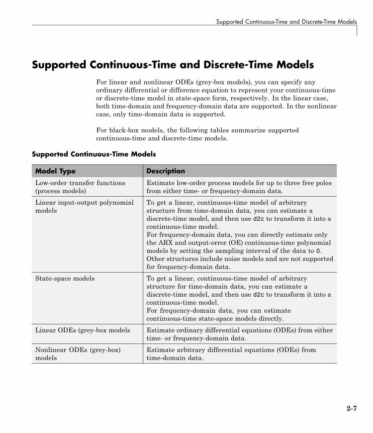
Supported Continuous-Time and Discrete-Time Models
Supported Continuous-Time and Discrete-Time ModelsFor linear and nonlinear ODEs (grey-box models), you can specify anyordinary differential or difference equation to represent your continuous-timeor discrete-time model in state-space form, respectively. In the linear case,both time-domain and frequency-domain data are supported. In the nonlinearcase, only time-domain data is supported.
For black-box models, the following tables summarize supportedcontinuous-time and discrete-time models.
Supported Continuous-Time Models
Model Type Description
Low-order transfer functions(process models)
Estimate low-order process models for up to three free polesfrom either time- or frequency-domain data.
Linear input-output polynomialmodels
To get a linear, continuous-time model of arbitrarystructure from time-domain data, you can estimate adiscrete-time model, and then use d2c to transform it into acontinuous-time model.For frequency-domain data, you can directly estimate onlythe ARX and output-error (OE) continuous-time polynomialmodels by setting the sampling interval of the data to 0.Other structures include noise models and are not supportedfor frequency-domain data.
State-space models To get a linear, continuous-time model of arbitrarystructure for time-domain data, you can estimate adiscrete-time model, and then use d2c to transform it into acontinuous-time model.For frequency-domain data, you can estimatecontinuous-time state-space models directly.
Linear ODEs (grey-box models Estimate ordinary differential equations (ODEs) from eithertime- or frequency-domain data.
Nonlinear ODEs (grey-box)models
Estimate arbitrary differential equations (ODEs) fromtime-domain data.
2-7

2 Choosing Your System Identification Strategy
Supported Discrete-Time Models
Model Type Description
Linear, input-output polynomialmodels
Estimate arbitrary-order, linear parametric models fromtime- or frequency-domain data.To get a discrete-time model, your data sampling intervalmust be set to the (nonzero) value you used to sample inyour experiment.
Nonlinear black-box models Estimate from time-domain data only.Linear ODEs (grey-box) models Estimate ordinary difference equations from time- or
frequency-domain data.Nonlinear ODEs (grey-box)models
Estimate ordinary difference equations from time-domaindata.
2-8
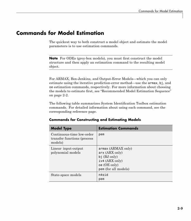
Commands for Model Estimation
Commands for Model EstimationThe quickest way to both construct a model object and estimate the modelparameters is to use estimation commands.
Note For ODEs (grey-box models), you must first construct the modelstructure and then apply an estimation command to the resulting modelobject.
For ARMAX, Box-Jenkins, and Output-Error Models—which you can onlyestimate using the iterative prediction-error method—use the armax, bj, andoe estimation commands, respectively. For more information about choosingthe models to estimate first, see “Recommended Model Estimation Sequence”on page 2-2.
The following table summarizes System Identification Toolbox estimationcommands. For detailed information about using each command, see thecorresponding reference page.
Commands for Constructing and Estimating Models
Model Type Estimation Commands
Continuous-time low-ordertransfer functions (processmodels)
pem
Linear input-outputpolynomial models
armax (ARMAX only)arx (ARX only)bj (BJ only)iv4 (ARX only)oe (OE only)pem (for all models)
State-space models n4sidpem
2-9

2 Choosing Your System Identification Strategy
Commands for Constructing and Estimating Models (Continued)
Model Type Estimation Commands
Linear time-series models ararx (for multiple outputs)ivar
Nonlinear ARX models nlarx
Hammerstein-Wienermodels
nlhw
2-10
Creating Model Structures at the Command Line
Creating Model Structures at the Command Line
In this section...
“About System Identification Toolbox Model Objects” on page 2-11“When to Construct a Model Structure Independently of Estimation” onpage 2-12“Commands for Constructing Model Structures” on page 2-13“Model Properties” on page 2-14“See Also” on page 2-20
About System Identification Toolbox Model ObjectsObjects are based on model classes. Each class is a blueprint that defines thefollowing information about your model:
• How the object stores data
• Which operations you can perform on the object
This toolbox includes nine classes for representing models. For example,idpoly represents linear input-output polynomial models, and idssrepresents linear state-space models. For a complete list of available modelobjects, see “Commands for Constructing Model Structures” on page 2-13.
Model properties define how a model object stores information. Model objectsstore information about a model, including the mathematical form of amodel, names of input and output channels, units, names and values ofestimated parameters, parameter uncertainties, algorithm specifications, andestimation information. For example, the idpoly model class has a propertycalled InputName for storing one or more input channel names. Differentmodel objects have different properties.
The allowed operations on an object are called methods. In the SystemIdentification Toolbox product, some methods have the same name but applyto multiple model objects. For example, the method bode creates a bode plotfor all linear model objects. However, other methods are unique to a specific
2-11

2 Choosing Your System Identification Strategy
model object. For example, the estimation method n4sid is unique to thestate-space model object idss.
Every class has a special method for creating objects of that class, called theconstructor. Using a constructor creates an instance of the correspondingclass or instantiates the object. The constructor name is the same as the classname. For example, idpoly is both the name of the class representing linearblack-box polynomial models and the name of the constructor for instantiatingthe model object.
For a tutorial about estimating models at the command line, see “Tutorial –Identifying Linear Models Using the Command Line” in System IdentificationToolbox Getting Started Guide.
When to Construct a Model Structure Independentlyof EstimationYou use model constructors to create a model object at the command line byspecifying all required model properties explicitly.
You must construct the model object independently of estimation when youwant to:
• Simulate a model
• Analyze a model
• Specify an initial guess for specific model parameter values beforeestimation
In most cases, you can use the estimation commands to both constructand estimate the model—without having to construct the model objectindependently. For example, the estimation command pem lets you specifyboth the model structure with unknown parameters and the estimationalgorithm. For information about how to both construct and estimate modelswith a single command, see “Commands for Model Estimation” on page 2-9.
In case of grey-box models, you must always construct the model object firstand then estimate the parameters of the ordinary differential or differenceequation. For more information, see Chapter 5, “ODE Parameter Estimation(Grey-Box Modeling)”.
2-12

Creating Model Structures at the Command Line
Commands for Constructing Model StructuresThe following table summarizes the model constructors available in theSystem Identification Toolbox product for representing various types ofmodels.
After model estimation, you can recognize the corresponding model objectsin the MATLAB Workspace browser by their class names. The name of theconstructor matches the name of the object it creates.
For information about how to both construct and estimate models with asingle command, see “Commands for Model Estimation” on page 2-9.
Summary of Model Constructors
Model Constructor Resulting Model Class Single or Multiple Outputs?
idarx Parametric multiple-outputARX models. Alsorepresents nonparametrictransient-response models.
Single- or multiple-outputmodels.
idfrd Nonparametricfrequency-response model.
Single- or multiple-outputmodels.
idproc Continuous-time, low-ordertransfer functions (processmodels).
Single-output models only.
idpoly Linear input-output polynomialmodels:
• ARX
• ARMAX
• Output-Error
• Box-Jenkins
Single-output models only.
idss Linear state-space models. Single- or multiple-outputmodels.
2-13
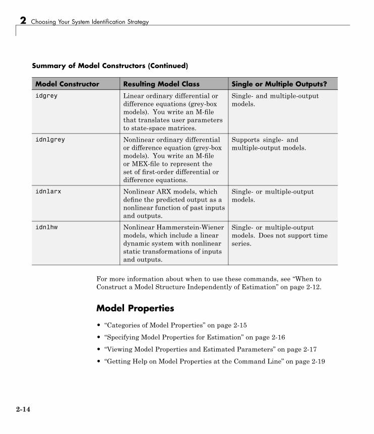
2 Choosing Your System Identification Strategy
Summary of Model Constructors (Continued)
Model Constructor Resulting Model Class Single or Multiple Outputs?
idgrey Linear ordinary differential ordifference equations (grey-boxmodels). You write an M-filethat translates user parametersto state-space matrices.
Single- and multiple-outputmodels.
idnlgrey Nonlinear ordinary differentialor difference equation (grey-boxmodels). You write an M-fileor MEX-file to represent theset of first-order differential ordifference equations.
Supports single- andmultiple-output models.
idnlarx Nonlinear ARX models, whichdefine the predicted output as anonlinear function of past inputsand outputs.
Single- or multiple-outputmodels.
idnlhw Nonlinear Hammerstein-Wienermodels, which include a lineardynamic system with nonlinearstatic transformations of inputsand outputs.
Single- or multiple-outputmodels. Does not support timeseries.
For more information about when to use these commands, see “When toConstruct a Model Structure Independently of Estimation” on page 2-12.
Model Properties
• “Categories of Model Properties” on page 2-15
• “Specifying Model Properties for Estimation” on page 2-16
• “Viewing Model Properties and Estimated Parameters” on page 2-17
• “Getting Help on Model Properties at the Command Line” on page 2-19
2-14

Creating Model Structures at the Command Line
Categories of Model PropertiesThe way a model object stores information is defined by the properties of thecorresponding model class.
Each model object has properties for storing information that are relevantonly to that specific model type. However, the idarx, idgrey, idpoly, idproc,and idss model objects are based on the idmodel superclass and inherit allidmodel properties.
Similarly, the nonlinear models idnlarx, idnlhw, and idnlgrey are based onthe idnlmodel superclass and inherit all idnlmodel properties.
In general, all nonlinear model objects have properties that belong to thefollowing categories:
• Names of input and output channels, such as InputName and OutputName
• Sampling interval of the model, such as Ts
• Units for time or frequency
• Model order and mathematical structure (for example, ODE ornonlinearities)
• Properties that store estimation results and model uncertainty
• User comments, such as Notes and Userdata
• Estimation algorithm information
- Algorithm
Structure includes fields that specify the estimation method. Algorithmincludes another structure, called Advanced, which provides additionalflexibility for setting the search algorithm. Different fields apply todifferent estimation techniques.
For linear parametric models, Algorithm specifies the frequencyweighing of the estimation using the Focus property.
Note Algorithm does not apply to idfrd models.
2-15

2 Choosing Your System Identification Strategy
- EstimationInfo
Structure includes read-only fields that describe the estimation data set,quantitative model quality measures, search termination conditions,how the initial states are handled, and any warnings encountered duringthe estimation.
For information about getting help on object properties, see “Getting Help onModel Properties at the Command Line” on page 2-19.
Specifying Model Properties for EstimationIf you are estimating a new model, you can specify model properties directlyin the estimator syntax. For a complete list of model estimation commands,see “Commands for Model Estimation” on page 2-9.
When using the commands that let you both construct and estimate a model,you can specify all top-level model properties in the estimator syntax.Top-level properties are those listed when you type get(object_name). Youcan also specify the top-level fields of the Algorithm structure directly inthe estimator using property-value pairs—such as focus in the previousexample—without having to define the structure fields first.
The following commands load the sample data, z8, construct an ARMAXmodel, and estimate the model parameters. The arguments of the armaxestimator specify model properties as property-value pairs.
load iddata8m_armax=armax(z8,'na',4,...
'nb',[3 2 3],...'nc',4,...'nk',[0 0 0],...'focus', 'simulation',...'covariance', 'none',...'tolerance',1e-5,...'maxiter',50);
focus, covariance, tolerance, and maxiter are fields in the Algorithmmodel property and specify aspects of the estimation algorithm.
2-16

Creating Model Structures at the Command Line
For linear models, you can use a shortcut to specify the second-levelAlgorithm properties, such as Advanced. With this syntax, you can referencethe structure fields by name without specifying the structure to which thesefields belong.
However, when estimating nonlinear black-box models, you must set thespecific fields of the Advanced Algorithm structure and the nonlinearityestimators before estimation. For example, suppose you want to set the valueof the wavenet object property Options, which is a structure. The followingcommands set the Options values before estimation and include the modifiedwavenet object in the estimator:
% Define wavenet object with defaul propertiesW = wavenet;% Specify variable to represent Options fieldO = W.Options;% Modify values of specific Options fieldsO.MaxLevels = 5 ;O.DilationStep = 2;% Estimate model using new Options settingsM = nlarx(data,[2 2 1],wavenet('options',O))
where O specifies the values of the Options structure fields and M is theestimated model. For more information about these and other commands,see the corresponding reference page.
Viewing Model Properties and Estimated ParametersTo view all the properties and values of any model object, use the getcommand. For example, type the following at the prompt to load sample data,compute an ARX model, and list the model properties:
load iddata8m_arx=arx(z8,[4 3 2 3 0 0 0]);get(m_arx)
To access a specific property, use dot notation. For example, to view theA matrix containing the estimated parameters in the previous model, typethe following command:
m_arx.a
2-17
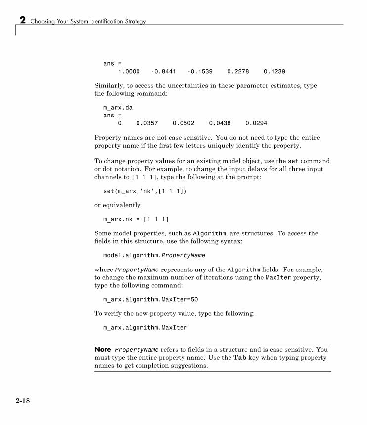
2 Choosing Your System Identification Strategy
ans =1.0000 -0.8441 -0.1539 0.2278 0.1239
Similarly, to access the uncertainties in these parameter estimates, typethe following command:
m_arx.daans =
0 0.0357 0.0502 0.0438 0.0294
Property names are not case sensitive. You do not need to type the entireproperty name if the first few letters uniquely identify the property.
To change property values for an existing model object, use the set commandor dot notation. For example, to change the input delays for all three inputchannels to [1 1 1], type the following at the prompt:
set(m_arx,'nk',[1 1 1])
or equivalently
m_arx.nk = [1 1 1]
Some model properties, such as Algorithm, are structures. To access thefields in this structure, use the following syntax:
model.algorithm.PropertyName
where PropertyName represents any of the Algorithm fields. For example,to change the maximum number of iterations using the MaxIter property,type the following command:
m_arx.algorithm.MaxIter=50
To verify the new property value, type the following:
m_arx.algorithm.MaxIter
Note PropertyName refers to fields in a structure and is case sensitive. Youmust type the entire property name. Use the Tab key when typing propertynames to get completion suggestions.
2-18
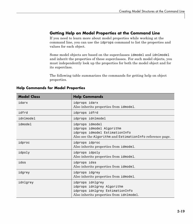
Creating Model Structures at the Command Line
Getting Help on Model Properties at the Command LineIf you need to learn more about model properties while working at thecommand line, you can use the idprops command to list the properties andvalues for each object.
Some model objects are based on the superclasses idmodel and idnlmodeland inherit the properties of these superclasses. For such model objects, youmust independently look up the properties for both the model object and forits superclass.
The following table summarizes the commands for getting help on objectproperties.
Help Commands for Model Properties
Model Class Help Commands
idarx idprops idarxAlso inherits properties from idmodel.
idfrd idprops idfrd
idnlmodel idprops idnlmodel
idmodel idprops idmodelidprops idmodel Algorithmidprops idmodel EstimationInfoAlso see the Algorithm and EstimationInfo reference page.
idproc idprops idprocAlso inherits properties from idmodel.
idpoly idprops idpolyAlso inherits properties from idmodel.
idss idprops idssAlso inherits properties from idmodel.
idgrey idprops idgreyAlso inherits properties from idmodel.
idnlgrey idprops idnlgreyidprops idnlgrey Algorithmidprops idnlgrey EstimationInfoAlso inherits properties from idnlmodel.
2-19

2 Choosing Your System Identification Strategy
Help Commands for Model Properties (Continued)
Model Class Help Commands
idnlarx idprops idnlarxidprops idnlarx Algorithmidprops idnlarx EstimationInfoAlso inherits properties from idnlmodel.
idnlhw idprops idnlhwidprops idnlhw Algorithmidprops idnlhw EstimationInfoAlso inherits properties from idnlmodel.
See AlsoValidate each model directly after estimation to help fine-tune your modelingstrategy. When you do not achieve a satisfactory model, you can try adifferent model structure and order, or try another identification algorithm.For more information about validating and troubleshooting models, seeChapter 8, “Model Analysis”.
After you have selected a good model to represent your system, see Chapter 9,“Simulation and Prediction”.
2-20

Modeling Multiple-Output Systems
Modeling Multiple-Output Systems
In this section...
“About Modeling Multiple-Output Systems” on page 2-21“Modeling Multiple Outputs Directly” on page 2-22“Modeling Multiple Outputs as a Combination of Single-Output Models”on page 2-22“Improving Multiple-Output Estimation Results by Weighing OutputsDuring Estimation” on page 2-23
About Modeling Multiple-Output SystemsYou can estimate multiple-output model directly using all the inputs andoutputs, or you can try building models for subsets of the most importantinput and output channels. To learn more about each approach, see:
• “Modeling Multiple Outputs Directly” on page 2-22
• “Modeling Multiple Outputs as a Combination of Single-Output Models”on page 2-22
Modeling multiple-output systems is more challenging because input/outputcouplings require additional parameters to obtain a good fit and involve morecomplex models. In general, a model is better when more data inputs areincluded during modeling. Including more outputs typically leads to worsesimulation results because it is harder to reproduce the behavior of severaloutputs simultaneously.
If you know that some of the outputs have poor accuracy and should beless important during estimation, you can control how much each outputis weighed in the estimation. For more information, see “ImprovingMultiple-Output Estimation Results by Weighing Outputs DuringEstimation” on page 2-23.
2-21

2 Choosing Your System Identification Strategy
Modeling Multiple Outputs DirectlyYou can estimate the following types of models for multiple-output data:
• Impulse- and step-response models
• Frequency-response models
• Linear ARX models
• State-space models
• Nonlinear ARX and Hammerstein-Wiener models
• Linear and nonlinear ODEs
Tip Estimating multiple-output state-space models directly generallyproduces better results than estimating other types of multiple-output modelsdirectly.
Modeling Multiple Outputs as a Combination ofSingle-Output ModelsYou may find that it is harder for a single model to explain the behavior ofseveral outputs. If you get a poor fit estimating a multiple-output modeldirectly, you can try building models for subsets of the most important inputand output channels.
Use this approach when no feedback is present in the dynamic system andthere are no couplings between the outputs. If you are unsure about thepresence of feedback, see “Getting Advice About Your Data” on page 1-84.
To construct partial models, use subreferencing to create partial data sets,such that each data set contains all inputs and one output. For moreinformation about creating partial data sets, see the following sections in theSystem Identification Toolbox User’s Guide:
• For working in the System Identification Tool GUI, see “Creating Data Setsfrom a Subset of Signal Channels” on page 1-31.
• For working at the command line, see the “Subreferencing iddata Objects”on page 1-55.
2-22

Modeling Multiple-Output Systems
After validating the single-output models, use vertical concatenation tocombine these partial models into a single multiple-output model. For moreinformation about concatenation, see “Concatenating iddata Objects” on page1-65 or “Concatenating idfrd Objects” on page 1-71.
You can try refining the concatenated multiple-output model using theoriginal (multiple-output) data set.
Improving Multiple-Output Estimation Results byWeighing Outputs During EstimationWhen estimating linear and nonlinear black-box models for multiple-outputsystems, you can control the relative importance of output channels duringthe estimation process. The ability to control how much each output isweighed during estimation is useful when some of the measured outputshave poor accuracy or should be treated as less important during estimation.For example, if you have already modeled one output well, you might wantto focus the estimation on modeling the remaining outputs. Similarly, youmight want to refine a model for a subset of outputs.
You can specify output weights directly in the estimation command usingthe Criterion and Weighting fields of the Algorithm property. You mustset the Criterion field to Trace, and set the Weighting field to the matrixthat contains the output weights. The Trace criterion minimizes the weightedsum of the prediction errors using the weights specified by Weighting.
The following code snippet shows how to specify the Criterion and WeightingAlgorithm fields as part of the pem command:
model=pem(z,2,'criterion','trace','weighting',diag(Q,1))
where Q is a vector of positive values and the higher values for outputs to beemphasized more during estimation.
You set Weighting to a positive semi-definite symmetric matrix of size equalto number of outputs. By default, Weighting is an identity matrix, whichmeans that all outputs are weighed equally during estimation.
For more information about these Algorithm fields for linear estimation, seethe Algorithm Properties reference page. For more information about
2-23

2 Choosing Your System Identification Strategy
the Algorithm fields for nonlinear estimation, see the idnlarx and idnlhwreference pages.
Note For multiple-output idnlarx models containing neuralnet ortreepartition nonlinearity estimators, output weighting is ignored becauseeach output is estimated independently.
2-24

3
Linear Model Identification
• “Identifying Frequency-Response Models” on page 3-2
• “Identifying Impulse-Response Models” on page 3-14
• “Identifying Low-Order Transfer Functions (Process Models)” on page 3-22
• “Identifying Input-Output Polynomial Models” on page 3-41
• “Identifying State-Space Models” on page 3-73
• “Refining Linear Parametric Models” on page 3-103
• “Extracting Parameter Values from Linear Models” on page 3-108
• “Extracting Dynamic Model and Noise Model Separately” on page 3-110
• “Transforming Between Discrete-Time and Continuous-TimeRepresentations” on page 3-112
• “Transforming Between Linear Model Representations” on page 3-117
• “Subreferencing Model Objects” on page 3-119
• “Concatenating Model Objects” on page 3-124
• “Merging Model Objects” on page 3-128

3 Linear Model Identification
Identifying Frequency-Response Models
In this section...
“What Is a Frequency-Response Model?” on page 3-2“Data Supported by Frequency-Response Models” on page 3-3“How to Estimate Frequency-Response Models in the GUI” on page 3-3“How to Estimate Frequency-Response Models at the Command Line” onpage 3-5“Options for Computing Spectral Models” on page 3-5“Options for Frequency Resolution” on page 3-6“Spectral Analysis Algorithm” on page 3-8“Understanding Spectrum Normalization” on page 3-11
What Is a Frequency-Response Model?You can estimate frequency-response models and visualize the responses ona Bode plot, which shows the amplitude change and the phase shift as afunction of the sinusoid frequency.
For a discrete-time system sampled with a time interval T, thefrequency-response model G(z) relates the Z-transforms of the input U(z)and output Y(z):
Y z G z U z( ) ( ) ( )=
The frequency-response function describes the steady-state response of asystem to sinusoidal inputs. For a linear system, a sinusoidal input of aspecific frequency results in an output that is also a sinusoid with the samefrequency, but with a different amplitude and phase. The frequency responsedescribes the amplitude change and phase shift as a function of frequency.
In other words, the frequency-response function, G(eiwT), is the Laplacetransform of the impulse response that is evaluated on the imaginary axis.The frequency-response function is the transfer function G(z) evaluated onthe unit circle.
3-2

Identifying Frequency-Response Models
Data Supported by Frequency-Response ModelsYou can estimate spectral analysis models from data with the followingcharacteristics:
• Complex or real data.
• Time- or frequency-domain iddata or idfrd data object. To learn moreabout estimating time-series models, see Chapter 6, “Time Series ModelIdentification”.
• Single- or multiple-output data.
How to Estimate Frequency-Response Models in theGUIYou must have already imported your data into the GUI and performed anynecessary preprocessing operations. For more information, see Chapter1, “Data Processing”.
To estimate frequency-response models in the System Identification Tool GUI:
1 In the System Identification Tool GUI, select Estimate > Spectralmodels to open the Spectral Model dialog box.
2 In the Method list, select the spectral analysis method you want to use.For information about each method, see “Options for Computing SpectralModels” on page 3-5.
3 Specify the frequencies at which to compute the spectral model in one ofthe following ways:
• In the Frequencies field, enter either a vector of values, a MATLABexpression that evaluates to a vector, or a variable name of a vector inthe MATLAB workspace. For example, logspace(-1,2,500).
• Use the combination of Frequency Spacing and Frequencies toconstruct the frequency vector of values:
– In the Frequency Spacing list, select Linear or Logarithmicfrequency spacing.
3-3
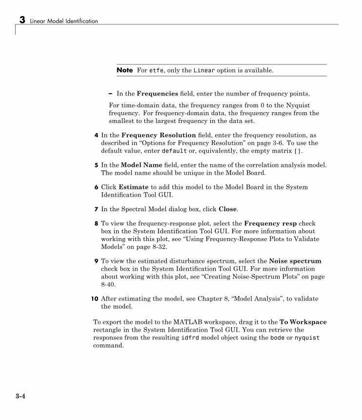
3 Linear Model Identification
Note For etfe, only the Linear option is available.
– In the Frequencies field, enter the number of frequency points.
For time-domain data, the frequency ranges from 0 to the Nyquistfrequency. For frequency-domain data, the frequency ranges from thesmallest to the largest frequency in the data set.
4 In the Frequency Resolution field, enter the frequency resolution, asdescribed in “Options for Frequency Resolution” on page 3-6. To use thedefault value, enter default or, equivalently, the empty matrix [].
5 In theModel Name field, enter the name of the correlation analysis model.The model name should be unique in the Model Board.
6 Click Estimate to add this model to the Model Board in the SystemIdentification Tool GUI.
7 In the Spectral Model dialog box, click Close.
8 To view the frequency-response plot, select the Frequency resp checkbox in the System Identification Tool GUI. For more information aboutworking with this plot, see “Using Frequency-Response Plots to ValidateModels” on page 8-32.
9 To view the estimated disturbance spectrum, select the Noise spectrumcheck box in the System Identification Tool GUI. For more informationabout working with this plot, see “Creating Noise-Spectrum Plots” on page8-40.
10 After estimating the model, see Chapter 8, “Model Analysis”, to validatethe model.
To export the model to the MATLAB workspace, drag it to the To Workspacerectangle in the System Identification Tool GUI. You can retrieve theresponses from the resulting idfrd model object using the bode or nyquistcommand.
3-4

Identifying Frequency-Response Models
How to Estimate Frequency-Response Models at theCommand LineYou can use the etfe, spa, and spafdr commands to estimate spectralmodels. The following table provides a brief description of each commandand usage examples.
The resulting models are stored as idfrd model objects. For detailedinformation about the commands and their arguments, see the correspondingreference page.
Commands for Frequency Response
Command Description Usage
etfe Estimates an empiricaltransfer function usingFourier analysis.
To estimate a model m, use the following syntax:
m=etfe(data)
spa Estimates a frequencyresponse with a fixedfrequency resolutionusing spectral analysis.
To estimate a model m, use the following syntax:
m=spa(data)
spafdr Estimates a frequencyresponse with a variablefrequency resolutionusing spectral analysis.
To estimate a model m, use the following syntax:
m=spafdr(data,R,w)
where R is the resolution vector and w is the frequencyvector.
After estimating the model, see Chapter 8, “Model Analysis” to validate themodel.
Options for Computing Spectral ModelsThis section describes how to select the method for computing spectral modelsin the estimation procedures “How to Estimate Frequency-Response Modelsin the GUI” on page 3-3 and “How to Estimate Frequency-Response Modelsat the Command Line” on page 3-5.
3-5

3 Linear Model Identification
You can choose from the following three spectral-analysis methods:
• etfe (Empirical Transfer Function Estimate)
For input-output data. This method computes the ratio of the Fouriertransform of the output to the Fourier transform of the input.
For time-series data. This method computes a periodogram as thenormalized absolute squares of the Fourier transform of the time series.
ETFE works well for highly resonant systems or narrowband systems.The drawback of this method is that it requires linearly spaced frequencyvalues, does not estimate the disturbance spectrum, and does not provideconfidence intervals. ETFE also works well for periodic inputs andcomputes exact estimates at multiples of the fundamental frequency of theinput and their ratio.
• spa (SPectral Analysis)
This method is the Blackman-Tukey spectral analysis method, wherewindowed versions of the covariance functions are Fourier transformed.For more information about this algorithm, see “Spectral AnalysisAlgorithm” on page 3-8.
• spafdr (SPectral Analysis with Frequency Dependent Resolution)
This method is a variant of the Blackman-Tukey spectral analysis methodwith frequency-dependent resolution. First, the algorithm computesFourier transforms of the inputs and outputs. Next, the products of thetransformed inputs and outputs with the conjugate input transform aresmoothed over local frequency regions. The widths of the local frequencyregions can vary as a function of frequency. The ratio of these averagescomputes the frequency-response estimate.
Options for Frequency Resolution
• “What Is Frequency Resolution?” on page 3-7
• “Frequency Resolution for etfe and spa” on page 3-7
• “Frequency Resolution for spafdr” on page 3-7
• “etfe Frequency Resolution for Periodic Input” on page 3-8
3-6

Identifying Frequency-Response Models
This section supports the estimation procedures “How to EstimateFrequency-Response Models in the GUI” on page 3-3 and “How to EstimateFrequency-Response Models at the Command Line” on page 3-5.
What Is Frequency Resolution?Frequency resolution is the size of the smallest frequency for which detailsin the frequency response and the spectrum can be resolved by the estimate.A resolution of 0.1 rad/s means that the frequency response variations atfrequency intervals at or below 0.1 rad/s are not resolved.
Note Finer resolution results in greater uncertainty in the model estimate.
Specifying the frequency resolution for etfe and spa is different than forspafdr.
Frequency Resolution for etfe and spaFor etfe and spa, the frequency resolution is approximately equal to thefollowing value:
2πM
radianssampling interval
⎛
⎝⎜
⎞
⎠⎟
M is a scalar integer that sets the size of the lag window.
A large value of M gives good resolution, but results in mode uncertainestimates.
The default value of M for spa is good for systems without sharp resonances.
For etfe, the default value of M gives the maximum resolution.
Frequency Resolution for spafdrIn case of etfe and spa, the frequency response is defined over a uniformfrequency range, 0-Fs/2 radians per second, where Fs is the samplingfrequency—equal to twice the Nyquist frequency. In contrast, spafdr lets
3-7
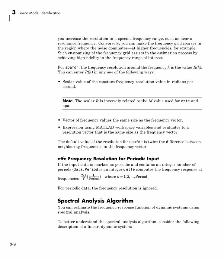
3 Linear Model Identification
you increase the resolution in a specific frequency range, such as near aresonance frequency. Conversely, you can make the frequency grid coarser inthe region where the noise dominates—at higher frequencies, for example.Such customizing of the frequency grid assists in the estimation process byachieving high fidelity in the frequency range of interest.
For spafdr, the frequency resolution around the frequency k is the value R(k).You can enter R(k) in any one of the following ways:
• Scalar value of the constant frequency resolution value in radians persecond.
Note The scalar R is inversely related to the M value used for etfe andspa.
• Vector of frequency values the same size as the frequency vector.
• Expression using MATLAB workspace variables and evaluates to aresolution vector that is the same size as the frequency vector.
The default value of the resolution for spafdr is twice the difference betweenneighboring frequencies in the frequency vector.
etfe Frequency Resolution for Periodic InputIf the input data is marked as periodic and contains an integer number ofperiods (data.Period is an integer), etfe computes the frequency response at
frequencies2 1 2πkT kk
Period where Period( ) = , ,..., .
For periodic data, the frequency resolution is ignored.
Spectral Analysis AlgorithmYou can estimate the frequency-response function of dynamic systems usingspectral analysis.
To better understand the spectral analysis algorithm, consider the followingdescription of a linear, dynamic system:
3-8

Identifying Frequency-Response Models
y t G q u t v t( ) ( ) ( ) ( )= +
where u(t) and y(t) are the input and output signals, respectively. G(q) iscalled the transfer function of the system—it takes the input to the outputand captures the system dynamics. The G(q)u(t) notation represents thefollowing operation:
G q u t g k u t kk
( ) ( ) ( ) ( )= −=
∞
∑1
q is the shift operator, defined by the following equation:
G q g k q q u t u tk
k
( ) ( ) ( ) ( )= = −−
=
∞−∑
1
1 1
G(q) that is evaluated on the unit circle, G(q=eiw), is the frequency-responsefunction.
Together, G(q=eiw) and the output noise spectrum ˆ ( )Φv ω comprise thefrequency-domain description of the system.
According to the Blackman-Tukey approach, the estimated frequency-responsefunction is given by the following equation:
ˆˆ
ˆG eNi yu
u
ω ω
ω( ) = ( )( )
Φ
Φ
In this case, ^ represents approximate quantities. For a derivation of thisequation, see the chapter on nonparametric time- and frequency-domainmethods in System Identification: Theory for the User, Second Edition, byLennart Ljung, Prentice Hall PTR, 1999.
The output noise spectrum is given by the following equation:
3-9

3 Linear Model Identification
ˆ ˆˆ
ˆΦ ΦΦ
Φv yyu
uω ω
ω
ω( ) = ( ) −
( )( )
2
This equation for the noise spectrum is derived by assuming the linearrelationship y t G q u t v t( ) ( ) ( ) ( )= + , that u(t) is independent of v(t), and thefollowing relationships between the spectra:
Φ Φ Φyi
u vG e( ) ( ) ( )ω ω ωω= ( ) +2
Φ Φyui
uG e( ) ( )ω ωω= ( )where the noise spectrum is given by the following equation:
Φv viwR e( ) ( )ω τ
τ
τ≡=−∞
∞−∑
ˆ ( )Φ yu ω is the output-input cross-spectrum andˆ ( )Φu ω is the input spectrum.
The algorithms for estimating the frequency response (such as spa) performthe following steps:
1 Compute the covariances and cross-covariance from u(t) and y(t), as follows:
ˆ
ˆ
ˆ
R y t y t
R u t u t
R
y Nt
N
u Nt
N
yu N
τ τ
τ τ
τ
( ) = +( ) ( )
( ) = +( ) ( )
( ) =
=
=
∑
∑
1
1
1
1
1 yy t u tt
N+( ) ( )
=∑ τ
1
3-10

Identifying Frequency-Response Models
2 Compute the Fourier transforms of the covariances and thecross-covariance, as follows:
ˆ ( ) ˆ ( ) ( )
ˆ ( ) ˆ ( ) ( )
Φ
Φ
y yM
M
Mi
u uM
M
Mi
R W e
R W e
ω τ τ
ω τ τ
τ
ωτ
τ
ωτ
=
=
=−
−
=−
−
∑
∑
ˆ ( ) ˆ ( ) ( )Φ yu yuM
M
MiR W eω τ τ
τ
ωτ==−
−∑
where WM ( )τ is called the lag window with the width M.
3 Compute the frequency-response function G eNiω( ) and the output noise
spectrum ˆ ( )Φv ω
Alternatively, the disturbance v(t) can be described as filtered white noise:
v t H q e t( ) ( ) ( )=
where e(t) is the white noise with variance λ and the noise power spectrumis given by the following equation:
ΦviH e( )ω λ ω= ( ) 2
Understanding Spectrum NormalizationThe spectrum of a signal is the square of the Fourier transform of thesignal. The spectral estimate using the commands spa, spafdr, and etfe isnormalized by the sampling interval T:
Φ y yk M
MiwT
MT R kT e W k( ) ( ) ( )ω ==−
−∑
3-11
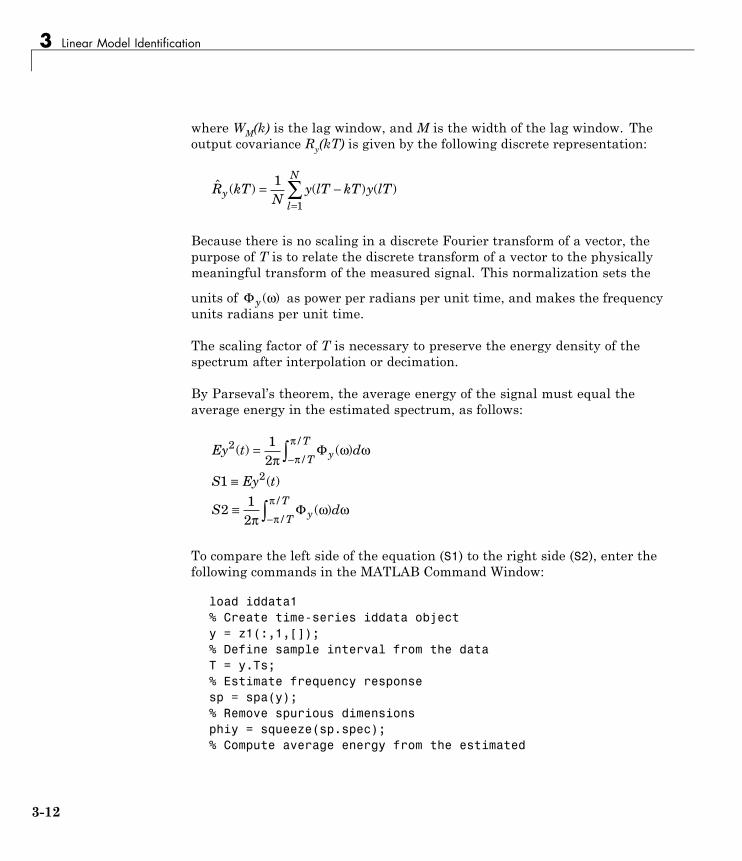
3 Linear Model Identification
where WM(k) is the lag window, and M is the width of the lag window. Theoutput covariance Ry(kT) is given by the following discrete representation:
ˆ ( ) ( ) ( )R kTN
y lT kT y lTyl
N= −
=∑1
1
Because there is no scaling in a discrete Fourier transform of a vector, thepurpose of T is to relate the discrete transform of a vector to the physicallymeaningful transform of the measured signal. This normalization sets the
units of Φ y ( )ω as power per radians per unit time, and makes the frequencyunits radians per unit time.
The scaling factor of T is necessary to preserve the energy density of thespectrum after interpolation or decimation.
By Parseval’s theorem, the average energy of the signal must equal theaverage energy in the estimated spectrum, as follows:
Ey t d
S Ey t
S d
yT
T
yT
T
2
2
12
1
212
( ) ( )
( )
( )
/
/
/
/
=
≡
≡
−
−
∫
∫
πω ω
πω ω
π
π
π
π
Φ
Φ
To compare the left side of the equation (S1) to the right side (S2), enter thefollowing commands in the MATLAB Command Window:
load iddata1% Create time-series iddata objecty = z1(:,1,[]);% Define sample interval from the dataT = y.Ts;% Estimate frequency responsesp = spa(y);% Remove spurious dimensionsphiy = squeeze(sp.spec);% Compute average energy from the estimated
3-12
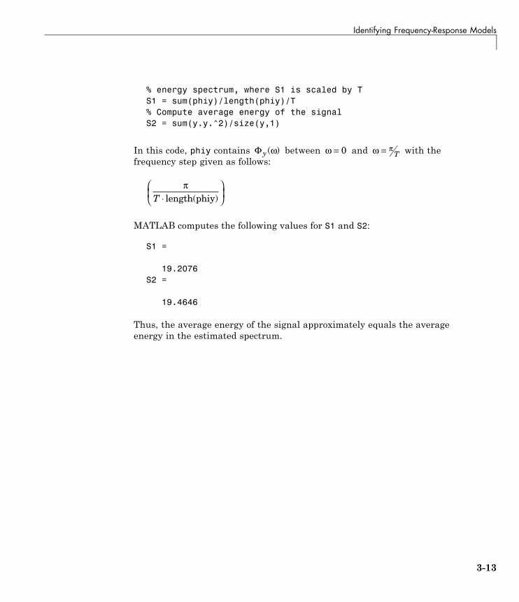
Identifying Frequency-Response Models
% energy spectrum, where S1 is scaled by TS1 = sum(phiy)/length(phiy)/T% Compute average energy of the signalS2 = sum(y.y.^2)/size(y,1)
In this code, phiy contains Φ y ( )ω between ω = 0 and ω π= T with thefrequency step given as follows:
πT ⋅
⎛
⎝⎜
⎞
⎠⎟length(phiy)
MATLAB computes the following values for S1 and S2:
S1 =
19.2076S2 =
19.4646
Thus, the average energy of the signal approximately equals the averageenergy in the estimated spectrum.
3-13

3 Linear Model Identification
Identifying Impulse-Response Models
In this section...
“What Is Time-Domain Correlation Analysis?” on page 3-14“Data Supported by Correlation Analysis” on page 3-15“How to Estimate Correlation Models Using the GUI” on page 3-15“How to Estimate Correlation Models at the Command Line” on page 3-16“How to Compute Response Values” on page 3-18“How to Identify Delay Using Transient-Response Plots” on page 3-18“Algorithm for Correlation Analysis” on page 3-20
What Is Time-Domain Correlation Analysis?Time-domain correlation analysis is a nonparametric estimate of transientresponse of dynamic systems, which computes a finite impulse response (FIR)model from the data. Correlation analysis assumes a linear system and doesnot require a specific model structure.
There are two types of transient response for a dynamic model:
• Impulse response
Impulse response is the output signal that results when the input is animpulse and has the following definition for a discrete model:
u t tu t t
( )( )
= >= =
0 01 0
• Step response
Step response is the output signal that results from a step input, defined asfollows:
u t tu t t
( )( )
= <= ≥
0 01 0
3-14
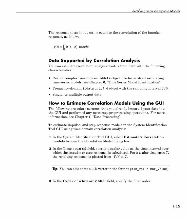
Identifying Impulse-Response Models
The response to an input u(t) is equal to the convolution of the impulseresponse, as follows:
y t h t z u z dzt
( ) ( )= −( ) ⋅∫0
Data Supported by Correlation AnalysisYou can estimate correlation analysis models from data with the followingcharacteristics:
• Real or complex time-domain iddata object. To learn about estimatingtime-series models, see Chapter 6, “Time Series Model Identification”.
• Frequency-domain iddata or idfrd object with the sampling interval T≠0.
• Single- or multiple-output data.
How to Estimate Correlation Models Using the GUIThe following procedure assumes that you already imported your data intothe GUI and performed any necessary preprocessing operations. For moreinformation, see Chapter 1, “Data Processing”.
To estimate impulse- and step-response models in the System IdentificationTool GUI using time-domain correlation analysis:
1 In the System Identification Tool GUI, select Estimate > Correlationmodels to open the Correlation Model dialog box.
2 In the Time span (s) field, specify a scalar value as the time interval overwhich the impulse or step response is calculated. For a scalar time span T,the resulting response is plotted from -T/4 to T.
Tip You can also enter a 2-D vector in the format [min_value max_value].
3 In the Order of whitening filter field, specify the filter order.
3-15

3 Linear Model Identification
The prewhitening filter is determined by modeling the input as anAuto-Regressive (AR) process of order N. The algorithm applies a filter ofthe form A(q)u(t)=u_F(t). That is, the input u(t) is subjected to an FIRfilter A to produce the filtered signal u_F(t). Prewhitening the input byapplying a whitening filter before estimation might improve the quality ofthe estimated impulse response g.
The order of the prewhitening filter, N, is the order of the A filter. N equalsthe number of lags. The default value of N is 10, which you can also specifyas [].
4 In theModel Name field, enter the name of the correlation analysis model.The name of the model should be unique in the Model Board.
5 Click Estimate to add this model to the Model Board in the SystemIdentification Tool GUI.
6 In the Correlation Model dialog box, click Close.
7 To view the transient response plot, select the Transient resp check boxin the System Identification Tool GUI. For more information about workingwith this plot and selecting to view impulse- versus step-response, see“Using Impulse- and Step-Response Plots to Validate Models” on page 8-24.
You can export the model to the MATLAB workspace for further analysisby dragging it to the To Workspace rectangle in the System IdentificationTool GUI.
How to Estimate Correlation Models at the CommandLineYou can use impulse and step commands to estimate the impulse and stepresponse directly from time- or frequency-domain data using correlationanalysis. Both impulse and step produce the same FIR model, but generatedifferent plots.
Note cra is an alternative method for computing impulse response fromtime-domain data only.
3-16

Identifying Impulse-Response Models
The following tables summarize the commands for computing impulse- andstep-response models. The resulting models are stored as idarx model objectsand contain impulse-response coefficients in the model parameter B. Fordetailed information about these commands, see the corresponding referencepage.
Commands for Impulse and Step Response
Command Description Example
impulse Estimates a high-order,noncausal FIR modelusing correlation analysis.
To estimate the model m and plot the impulseresponse, use the following syntax:
m=impulse(data,Time,'pw',N)
where data is a single- or multiple-outputtime-domain iddata object, and Time is ascalar value representing the time intervalover which the impulse or step response iscalculated. For a scalar time span T, theresulting response is plotted from -T/4 to T.'pw' and N is an option property-value pairthat specifies the order N of the prewhiteningfilter 'pw'.
step Estimates a high-order,noncausal FIR modelcorrelation analysis.
To estimate the model m and plot the stepresponse, use the following syntax:
step(data,Time)
where data is a single- or multiple-outputtime-domain iddata object, and Time is thetime span.
To validate the model, see Chapter 8, “Model Analysis”. For more informationabout continuing to work with models in the MATLAB workspace, seeChapter 11, “Using System Identification Toolbox Blocks”.
3-17
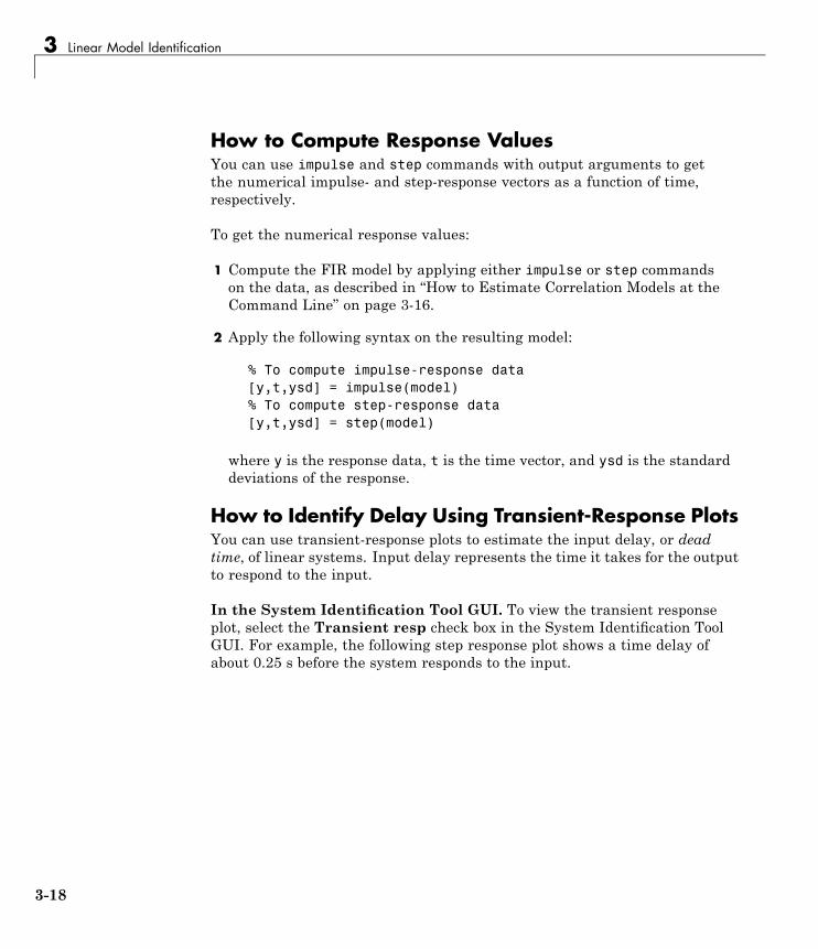
3 Linear Model Identification
How to Compute Response ValuesYou can use impulse and step commands with output arguments to getthe numerical impulse- and step-response vectors as a function of time,respectively.
To get the numerical response values:
1 Compute the FIR model by applying either impulse or step commandson the data, as described in “How to Estimate Correlation Models at theCommand Line” on page 3-16.
2 Apply the following syntax on the resulting model:
% To compute impulse-response data[y,t,ysd] = impulse(model)% To compute step-response data[y,t,ysd] = step(model)
where y is the response data, t is the time vector, and ysd is the standarddeviations of the response.
How to Identify Delay Using Transient-Response PlotsYou can use transient-response plots to estimate the input delay, or deadtime, of linear systems. Input delay represents the time it takes for the outputto respond to the input.
In the System Identification Tool GUI. To view the transient responseplot, select the Transient resp check box in the System Identification ToolGUI. For example, the following step response plot shows a time delay ofabout 0.25 s before the system responds to the input.
3-18

Identifying Impulse-Response Models
Step Response Plot
At the command line. You can use the impulse command to plot theimpulse response. The time delay is equal to the first positive peak in thetransient response magnitude that is greater than the confidence region forpositive time values.
For example, the following commands create an impulse-response plot with a1-standard-deviation confidence region:
% Load sample dataload dry2% Split data into estimation and% validation data setsze = dry2(1:500);zr = dry2(501:1000);impulse(ze,'sd',1,'fill')
The resulting figure shows that the first positive peak of the responsemagnitude, which is greater than the confidence region for positive timevalues, occurs at 0.24 s.
3-19

3 Linear Model Identification
Algorithm for Correlation AnalysisTo better understand the algorithm underlying correlation analysis, considerthe following description of a dynamic system:
y t G q u t v t( ) ( ) ( ) ( )= +
where u(t) and y(t) are the input and output signals, respectively. v(t) is theadditive noise term. G(q) is the transfer function of the system. The G(q)u(t)notation represents the following operation:
G q u t g k u t kk
( ) ( ) ( ) ( )= −=
∞
∑1
3-20

Identifying Impulse-Response Models
q is the shift operator, defined by the following equation:
G q g k q q u t u tk
k
( ) ( ) ( ) ( )= = −−
=
∞−∑
1
1 1
For impulse response, the algorithm estimates impulse response coefficientsg for both the single- and multiple-output data. The impulse response isestimated as a high-order, noncausal FIR model:
y t g m u t m g u t g u tg u t
( ) ( ) ( ) ( ) ( ) ( ) ( )( ) (
= − + + + − + ++ −
… 1 1 01 11) ( ) ( )+ + −… g n u t n
The estimation algorithm prefilters the data such that the input is as whiteas possible. It then computes the correlations from the prefiltered data toobtain the FIR coefficients.
g is also estimated for negative lags, which takes into account any noncausaleffects from input to output. Noncausal effects can result from feedback. Thecoefficients are computed using the least-squares method.
For a multiple-input or multiple-output system, the impulse response gk is anny-by-nu matrix, where ny is the number of outputs and nu is the numberof inputs. The i-jth element of the impulse response matrix describes thebehavior of the ith output after an impulse in the jth input.
3-21
3 Linear Model Identification
Identifying Low-Order Transfer Functions (Process Models)
In this section...
“What Is a Process Model?” on page 3-22“Data Supported by a Process Model” on page 3-23“How to Estimate Process Models Using the GUI” on page 3-23“Estimating Process Models at the Command Line” on page 3-29“Options for Specifying the Process-Model Structure” on page 3-35“Options for Multiple-Input Models” on page 3-36“Options for the Disturbance Model Structure” on page 3-37“Options for Frequency-Weighing Focus” on page 3-38“Options for Initial States” on page 3-39
What Is a Process Model?The structure of a continuous-time process model is a simple transfer functionthat describes linear system dynamics in terms of one or more of the followingelements:
• Static gain Kp.
• One or more time constants Tpk. For complex poles, the time constant iscalled Tω—equal to the inverse of the natural frequency—and the dampingcoefficient is ζ (zeta).
• Process zero Tz.
• Possible time delay Td before the system output responds to the input(dead time).
• Possible enforced integration.
Process models are popular for describing system dynamics in manyindustries and apply to various production environments. The primaryadvantages of these models are that they provide delay estimation, and themodel coefficients have a physical interpretation.
3-22
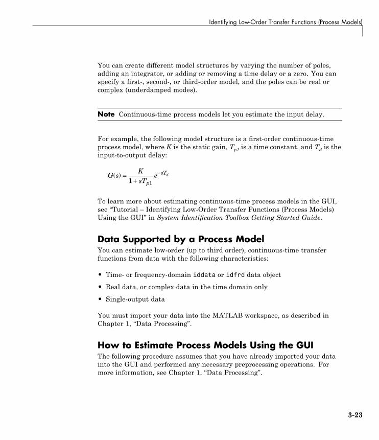
Identifying Low-Order Transfer Functions (Process Models)
You can create different model structures by varying the number of poles,adding an integrator, or adding or removing a time delay or a zero. You canspecify a first-, second-, or third-order model, and the poles can be real orcomplex (underdamped modes).
Note Continuous-time process models let you estimate the input delay.
For example, the following model structure is a first-order continuous-timeprocess model, where K is the static gain, Tp1 is a time constant, and Td is theinput-to-output delay:
G sKsT
ep
sTd( ) =+
−1 1
To learn more about estimating continuous-time process models in the GUI,see “Tutorial – Identifying Low-Order Transfer Functions (Process Models)Using the GUI” in System Identification Toolbox Getting Started Guide.
Data Supported by a Process ModelYou can estimate low-order (up to third order), continuous-time transferfunctions from data with the following characteristics:
• Time- or frequency-domain iddata or idfrd data object
• Real data, or complex data in the time domain only
• Single-output data
You must import your data into the MATLAB workspace, as described inChapter 1, “Data Processing”.
How to Estimate Process Models Using the GUIThe following procedure assumes that you have already imported your datainto the GUI and performed any necessary preprocessing operations. Formore information, see Chapter 1, “Data Processing”.
3-23

3 Linear Model Identification
To estimate a low-order transfer function (process model) using the SystemIdentification Tool GUI:
1 In the System Identification Tool GUI, select Estimate > Process modelsto open the Process Models dialog box.
2 If your model contains multiple inputs, select the input channel in theInput list. This list only appears when you have multiple inputs. For moreinformation, see “Options for Multiple-Input Models” on page 3-36.
3 In the Model Transfer Function area, specify the model structure usingthe following options:
3-24
Identifying Low-Order Transfer Functions (Process Models)
• Under Poles, select the number of poles, and then select All real orUnderdamped.
Note You need at least two poles to allow underdamped modes(complex-conjugate pair).
• Select the Zero check box to include a zero, which is a numerator termother than a constant, or clear the check box to exclude the zero.
• Select the Delay check box to include a delay, or clear the check boxto exclude the delay.
• Select the Integrator check box to include an integrator (self-regulatingprocess), or clear the check box to exclude the integrator.
The Parameter area shows as many active parameters as you included inthe model structure.
Note By default, the model Name is set to the acronym that reflects themodel structure, as described in “Options for Specifying the Process-ModelStructure” on page 3-35.
4 In the Initial Guess area, select Auto-selected to calculate the initialparameter values for the estimation. The Initial Guess column in the
3-25

3 Linear Model Identification
Parameter table displays Auto. If you do not have a good guess for theparameter values, Auto works better than entering an ad hoc value.
5 (Optional) If you approximately know a parameter value, enter this valuein the Initial Guess column of the Parameter table. The estimationalgorithm uses this value as a starting point. If you know a parametervalue exactly, enter this value in the Initial Guess column, and also selectthe corresponding Known check box in the table to fix its value.
If you know the range of possible values for a parameter, enter these valuesinto the corresponding Bounds field to help the estimation algorithm.
For example, the following figure shows that the delay value Td is fixedat 2 s and is not estimated.
3-26

Identifying Low-Order Transfer Functions (Process Models)
6 In the Disturbance Model list, select one of the available options. Formore information about each option, see “Options for the DisturbanceModel Structure” on page 3-37.
7 In the Focus list, select how to weigh the relative importance of the fit atdifferent frequencies. For more information about each option, see “Optionsfor Frequency-Weighing Focus” on page 3-38.
8 In the Initial state list, specify how you want the algorithm to treat initialstates. For more information about the available options, see “Options forInitial States” on page 3-39.
Tip If you get a bad fit, you might try setting a specific method for handlinginitial states, rather than choosing it automatically.
9 In the Covariance list, select Estimate if you want the algorithm tocompute parameter uncertainties. Effects of such uncertainties aredisplayed on plots as model confidence regions.
3-27

3 Linear Model Identification
To omit estimating uncertainty, select None. Skipping uncertaintycomputation might reduce computation time for complex models and largedata sets.
10 In the Model Name field, edit the name of the model or keep the default.The name of the model should be unique in the Model Board.
11 To view the estimation progress in the MATLAB Command Window, selectthe Trace check box. During estimation, the following information isdisplayed for each iteration:
• Loss function — Equals the determinant of the estimated covariancematrix of the input noise.
• Parameter values — Values of the model structure coefficients youspecified.
• Search direction — Change in parameter values from the previousiteration.
• Fit improvements — Shows the actual versus expected improvements inthe fit.
12 Click Estimate to add this model to the Model Board in the SystemIdentification Tool GUI.
13 To stop the search and save the results after the current iteration has beencompleted, click Stop Iterations. To continue iterations from the currentmodel, click the Continue iter button to assign current parameter valuesas initial guesses for the next search.
14 To plot the model, select the appropriate check box in the Model Viewsarea of the System Identification Tool GUI. For more information aboutvalidating models, see “Overview of Model Validation and Plots” on page8-2.
15 To refine the current estimate, click the Value —> Initial Guess buttonto assign current parameter values as initial guesses for the next search,edit the Model Name field, and click Estimate.
If your model is not sufficiently accurate, try another model structure.
3-28

Identifying Low-Order Transfer Functions (Process Models)
You can export the model to the MATLAB workspace for further analysisby dragging it to the To Workspace rectangle in the System IdentificationTool GUI.
Estimating Process Models at the Command Line
• “Using pem to Estimate Process Models” on page 3-29
• “Example – Estimating Process Models with Free Parameters at theCommand Line” on page 3-30
• “Example – Estimating Process Models with Fixed Parameters at theCommand Line” on page 3-32
Using pem to Estimate Process ModelsYou can estimate process models using the iterative estimation method pemthat minimizes the prediction errors to obtain maximum likelihood estimates.The resulting models are stored as idproc model objects.
You can use the following general syntax to both configure and estimateprocess models:
m = pem(data,mod_struc,'Property1',Value1,...,'PropertyN',ValueN)
data is the estimation data and mod_struc is a string that representsthe process model structure, as described in “Options for Specifying theProcess-Model Structure” on page 3-35.
Tip You do not need to construct the model object using idproc beforeestimation unless you want to specify initial parameter guesses or fixedparameter values, as described in “Example – Estimating Process Modelswith Fixed Parameters at the Command Line” on page 3-32.
The property-value pairs specify any model properties that configure theestimation algorithm and the initial conditions. For more information aboutaccessing and setting model properties, see “Model Properties” on page 2-14.
3-29
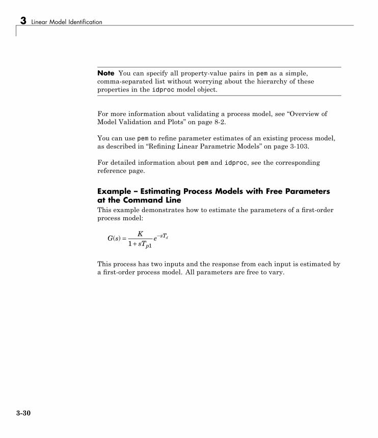
3 Linear Model Identification
Note You can specify all property-value pairs in pem as a simple,comma-separated list without worrying about the hierarchy of theseproperties in the idproc model object.
For more information about validating a process model, see “Overview ofModel Validation and Plots” on page 8-2.
You can use pem to refine parameter estimates of an existing process model,as described in “Refining Linear Parametric Models” on page 3-103.
For detailed information about pem and idproc, see the correspondingreference page.
Example – Estimating Process Models with Free Parametersat the Command LineThis example demonstrates how to estimate the parameters of a first-orderprocess model:
G sKsT
ep
sTd( ) =+
−1 1
This process has two inputs and the response from each input is estimated bya first-order process model. All parameters are free to vary.
3-30
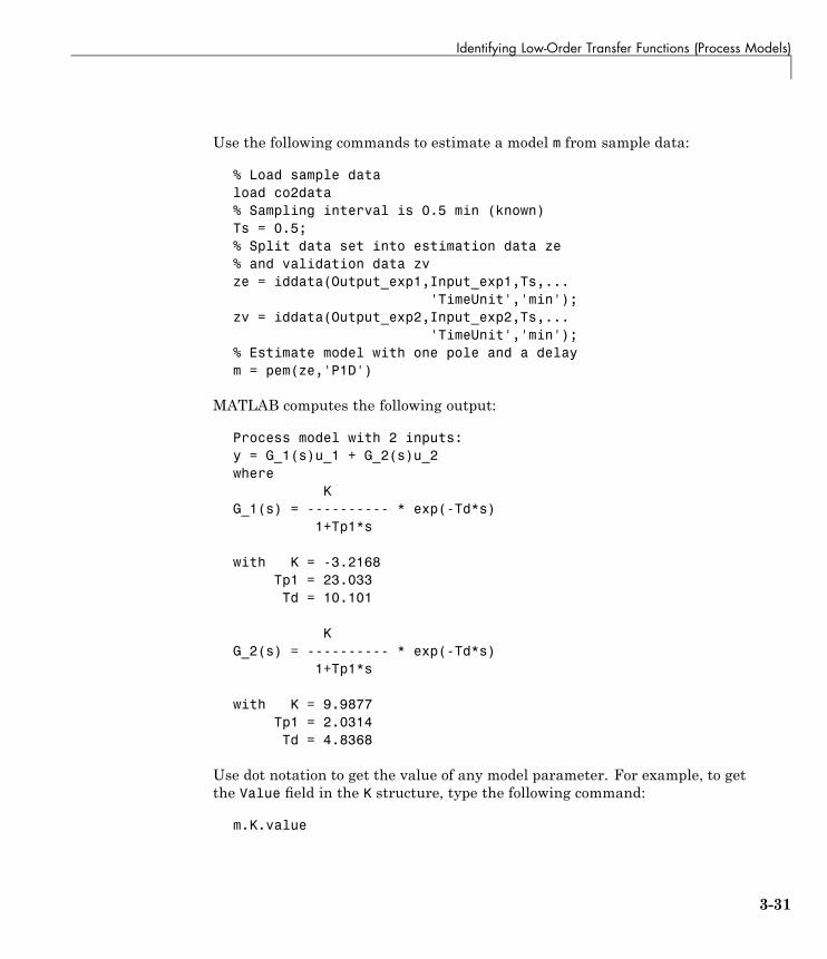
Identifying Low-Order Transfer Functions (Process Models)
Use the following commands to estimate a model m from sample data:
% Load sample dataload co2data% Sampling interval is 0.5 min (known)Ts = 0.5;% Split data set into estimation data ze% and validation data zvze = iddata(Output_exp1,Input_exp1,Ts,...
'TimeUnit','min');zv = iddata(Output_exp2,Input_exp2,Ts,...
'TimeUnit','min');% Estimate model with one pole and a delaym = pem(ze,'P1D')
MATLAB computes the following output:
Process model with 2 inputs:y = G_1(s)u_1 + G_2(s)u_2where
KG_1(s) = ---------- * exp(-Td*s)
1+Tp1*s
with K = -3.2168Tp1 = 23.033Td = 10.101
KG_2(s) = ---------- * exp(-Td*s)
1+Tp1*s
with K = 9.9877Tp1 = 2.0314Td = 4.8368
Use dot notation to get the value of any model parameter. For example, to getthe Value field in the K structure, type the following command:
m.K.value
3-31
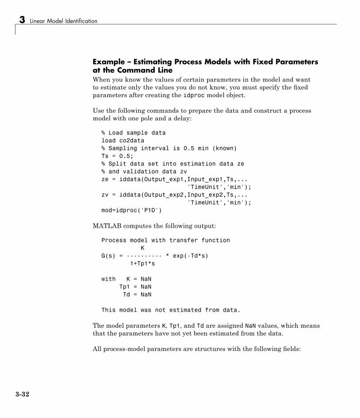
3 Linear Model Identification
Example – Estimating Process Models with Fixed Parametersat the Command LineWhen you know the values of certain parameters in the model and wantto estimate only the values you do not know, you must specify the fixedparameters after creating the idproc model object.
Use the following commands to prepare the data and construct a processmodel with one pole and a delay:
% Load sample dataload co2data% Sampling interval is 0.5 min (known)Ts = 0.5;% Split data set into estimation data ze% and validation data zvze = iddata(Output_exp1,Input_exp1,Ts,...
'TimeUnit','min');zv = iddata(Output_exp2,Input_exp2,Ts,...
'TimeUnit','min');mod=idproc('P1D')
MATLAB computes the following output:
Process model with transfer functionK
G(s) = ---------- * exp(-Td*s)1+Tp1*s
with K = NaNTp1 = NaNTd = NaN
This model was not estimated from data.
The model parameters K, Tp1, and Td are assigned NaN values, which meansthat the parameters have not yet been estimated from the data.
All process-model parameters are structures with the following fields:
3-32

Identifying Low-Order Transfer Functions (Process Models)
• status field specifies whether to estimate the parameter, or keep the initialvalue fixed (do not estimate), or set the value to zero. This field can havethe values 'estimate', 'fixed', or 'zero'. For more information, see“Options for Initial States” on page 3-39.
• min specifies the minimum bound on the parameter.
• max specifies the maximum bound on the parameter.
• value specifies the numerical value of the parameter, if known.
To set the value of K to 12 and keep it fixed, use the following commands:
mod.K.value=12;mod.K.status='fixed';
Note mod is defined for one input. This model is automatically adjustedto have a duplicate for each input.
To estimate Tp1 and Td only, use the following command:
mod_proc=pem(ze,mod)
3-33

3 Linear Model Identification
MATLAB computes the following result:
Process model with 2 inputs:y = G_1(s)u_1 + G_2(s)u_2where
KG_1(s) = ---------- * exp(-Td*s)
1+Tp1*s
with K = 12Tp1 = 7.0998e+007Td = 15
KG_2(s) = ---------- * exp(-Td*s)
1+Tp1*s
with K = 12Tp1 = 3.6962Td = 3.817
In this case, the value of K is fixed at 12, but Tp1 and Td are estimated.
3-34

Identifying Low-Order Transfer Functions (Process Models)
If you prefer to specify parameter constraints directly in the estimator syntax,the following table provides examples of pem commands.
Action Example
Fix the value of K to 12.m=pem(ze,'p1d','k','fix','k',12)
Initialize K for the iterative searchwithout fixing this value. m=pem(ze,'p1d','k',12)
Constrain the value of K between3 and 4. m=pem(ze,'p1d','k',...
{'min',3},'k',{'max',4})
Options for Specifying the Process-Model StructureThis section describes how to specify the model structure in the estimationprocedures “How to Estimate Process Models Using the GUI” on page 3-23and “Estimating Process Models at the Command Line” on page 3-29.
In the System Identification Tool GUI. Specify the model structure byselecting the number of real or complex poles, and whether to include a zero,delay, and integrator. The resulting transfer function is displayed in theProcess Models dialog box.
At the command line. Specify the model structure using an acronym thatincludes the following letters and numbers:
• (Required) P for a process model
• (Required) 0, 1, 2 or 3 for the number of poles
• (Optional) D to include a time-delay term e sTd−
• (Optional) Z to include a process zero (numerator term)
• (Optional) U to indicate possible complex-valued (underdamped) poles
• (Optional) I to indicate enforced integration
3-35

3 Linear Model Identification
Typically, you specify the model-structure acronym as a string argument inthe estimation command pem:
• pem(data,'P1D') to estimate the following structure:
G sKsT
ep
sTd( ) =+
−1 1
• pem(data,'P2ZU') to estimate the following structure:
G sK sT
s T s T
p z
w w( ) =
+( )+ +
1
1 2 2 2ζ
• pem(data,'P0ID') to estimate the following structure:
G sK
sep sTd( ) = −
• pem(data,'P3Z') to estimate the following structure:
G sK sT
sT sT sTp z
p p p( ) =
+( )+( ) +( ) +( )
1
1 1 11 2 3
For more information about estimating models , see “Estimating ProcessModels at the Command Line” on page 3-29.
Options for Multiple-Input ModelsIf your model contains multiple inputs, you can specify whether to estimatethe same transfer function for all inputs, or a different transfer functionfor each input. The information in this section supports the estimationprocedures “How to Estimate Process Models Using the GUI” on page 3-23and “Estimating Process Models at the Command Line” on page 3-29.
In the System Identification Tool GUI. To fit a data set with multipleinputs in the Process Models dialog box, configure the process model settingsfor one input at a time. When you finish configuring the model and the
3-36
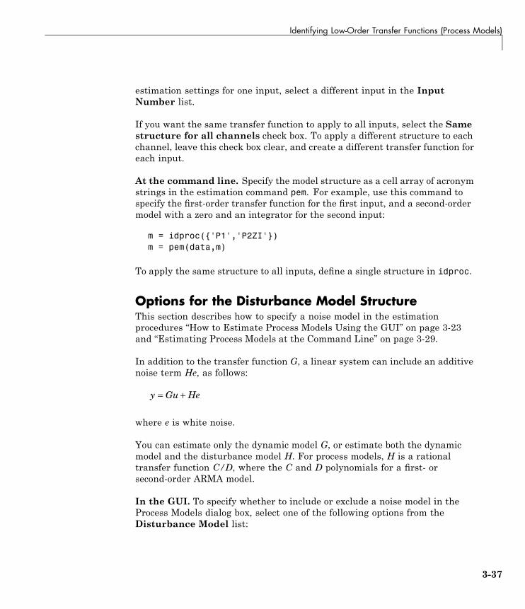
Identifying Low-Order Transfer Functions (Process Models)
estimation settings for one input, select a different input in the InputNumber list.
If you want the same transfer function to apply to all inputs, select the Samestructure for all channels check box. To apply a different structure to eachchannel, leave this check box clear, and create a different transfer function foreach input.
At the command line. Specify the model structure as a cell array of acronymstrings in the estimation command pem. For example, use this command tospecify the first-order transfer function for the first input, and a second-ordermodel with a zero and an integrator for the second input:
m = idproc({'P1','P2ZI'})m = pem(data,m)
To apply the same structure to all inputs, define a single structure in idproc.
Options for the Disturbance Model StructureThis section describes how to specify a noise model in the estimationprocedures “How to Estimate Process Models Using the GUI” on page 3-23and “Estimating Process Models at the Command Line” on page 3-29.
In addition to the transfer function G, a linear system can include an additivenoise term He, as follows:
y Gu He= +
where e is white noise.
You can estimate only the dynamic model G, or estimate both the dynamicmodel and the disturbance model H. For process models, H is a rationaltransfer function C/D, where the C and D polynomials for a first- orsecond-order ARMA model.
In the GUI. To specify whether to include or exclude a noise model in theProcess Models dialog box, select one of the following options from theDisturbance Model list:
3-37

3 Linear Model Identification
• None — The algorithm does not estimate a noise model (C=D=1). Thisoption also sets Focus to Simulation.
• Order 1 — Estimates a noise model as a continuous-time, first-orderARMA model.
• Order 2 — Estimates a noise model as a continuous-time, second-orderARMA model.
At the command line. Specify the disturbance model as an argument inthe estimation command pem. For example, use this command to estimate afirst-order transfer function and a first-order noise model:
pem(data,'P1D','DisturbanceModel','ARMA1')
Tip You can type 'dis' instead of 'DisturbanceModel'.
For a complete list of values for the DisturbanceModel model property, seethe idproc reference page.
Options for Frequency-Weighing FocusYou can specify how the estimation algorithm weighs the fit at variousfrequencies. This information supports the estimation procedures “How toEstimate Process Models Using the GUI” on page 3-23 and “EstimatingProcess Models at the Command Line” on page 3-29.
In the System Identification Tool GUI. Set Focus to one of the followingoptions:
• Prediction— Uses the inverse of the noise model H to weigh the relativeimportance of how closely to fit the data in various frequency ranges.Corresponds to minimizing one-step-ahead prediction, which typicallyfavors the fit over a short time interval. Optimized for output predictionapplications.
• Simulation— Uses the input spectrum to weigh the relative importance ofthe fit in a specific frequency range. Does not use the noise model to weighthe relative importance of how closely to fit the data in various frequencyranges. Optimized for output simulation applications.
3-38

Identifying Low-Order Transfer Functions (Process Models)
• Stability— Behaves the same way as the Prediction option, but alsoforces the model to be stable. For more information about model stability,see “Unstable Models” on page 8-69.
• Filter— Specify a custom filter to open the Estimation Focus dialog box,where you can enter a filter, as described in “Simple Passband Filter” onpage 1-111 or “Defining a Custom Filter” on page 1-112. This prefilteringapplies only for estimating the dynamics from input to output. Thedisturbance model is determined from the estimation data.
At the command line. Specify the focus as an argument in the estimationcommand pem using the same options as in the GUI. For example, use thiscommand to optimize the fit for simulation and estimate a disturbance model:
pem(data,'P1D','dist','arma2','Focus','Simulation')
Options for Initial StatesBecause the process models are dynamic, you need initial states thatcapture past input properties. Thus, you must specify how the iterativealgorithm treats initial states. This information supports the estimationprocedures “How to Estimate Process Models Using the GUI” on page 3-23and “Estimating Process Models at the Command Line” on page 3-29.
In the System Identification Tool GUI. Set Initial state to one of thefollowing options:
• Zero — Sets all initial states to zero.
• Estimate— Treats the initial states as an unknown vector of parametersand estimates these states from the data.
• Backcast — Estimates initial states using a backward filtering method(least-squares fit).
• U-level est — Estimates both the initial states and the InputLevelmodel property that represents the input offset level. For multiple inputs,the input level for each input is estimated individually. Use if you includedan integrator in the transfer function.
• Auto — Automatically chooses one of the preceding options based on theestimation data. If initial states have negligible effect on the predictionerrors, the initial states are set to zero to optimize algorithm performance.
3-39

3 Linear Model Identification
At the command line. Specify the initial states as an argument in theestimation command pem using the same options as in the GUI. For example,use this command to estimate a first-order transfer function and set theinitial states to zero:
m=pem(data,'P1D','InitialState','zero')
For a complete list of values for the InitialState model property, see theidproc reference page.
3-40
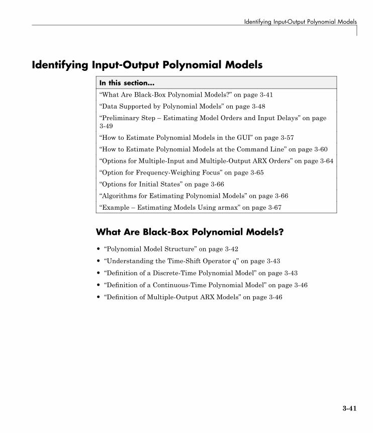
Identifying Input-Output Polynomial Models
Identifying Input-Output Polynomial Models
In this section...
“What Are Black-Box Polynomial Models?” on page 3-41“Data Supported by Polynomial Models” on page 3-48“Preliminary Step – Estimating Model Orders and Input Delays” on page3-49“How to Estimate Polynomial Models in the GUI” on page 3-57“How to Estimate Polynomial Models at the Command Line” on page 3-60“Options for Multiple-Input and Multiple-Output ARX Orders” on page 3-64“Option for Frequency-Weighing Focus” on page 3-65“Options for Initial States” on page 3-66“Algorithms for Estimating Polynomial Models” on page 3-66“Example – Estimating Models Using armax” on page 3-67
What Are Black-Box Polynomial Models?
• “Polynomial Model Structure” on page 3-42
• “Understanding the Time-Shift Operator q” on page 3-43
• “Definition of a Discrete-Time Polynomial Model” on page 3-43
• “Definition of a Continuous-Time Polynomial Model” on page 3-46
• “Definition of Multiple-Output ARX Models” on page 3-46
3-41

3 Linear Model Identification
Polynomial Model StructureYou can estimate the following types of linear polynomial model structures:
A q y tB qF q
u t nkC qD q
e ti
ii i
i
nu( ) ( )
( )( )
( )( )
( )= −( ) +=∑
1
The polynomials A, Bi, C, D, and F i contain the time-shift operator q. ui is theith input, nu is the total number of inputs, and nki is the ith input delay thatcharacterizes the delay response time. The variance of the white noise e(t)is assumed to be λ . For more information about the time-shift operator, see“Understanding the Time-Shift Operator q” on page 3-43.
Note This form is completely equivalent to the Z-transform form: qcorresponds to z.
To estimate polynomial models, you must specify the model order as a set ofintegers that represent the number of coefficients for each polynomial youinclude in your selected structure—na for A, nb for B, nc for C, nd for D,and nf for F. You must also specify the number of samples nk correspondingto the input delay—dead time—given by the number of samples before theoutput responds to the input.
The number of coefficients in denominator polynomials is equal to the numberof poles, and the number of coefficients in the numerator polynomials is equalto the number of zeros plus 1. When the dynamics from u(t) to y(t) contain adelay of nk samples, then the first nk coefficients of B are zero.
For more information about the family of transfer-function models, see thecorresponding section in System Identification: Theory for the User, SecondEdition, by Lennart Ljung, Prentice Hall PTR, 1999.
3-42

Identifying Input-Output Polynomial Models
Understanding the Time-Shift Operator qThe general polynomial equation is written in terms of the time-shift operatorq. To understand this time-shift operator, consider the following discrete-timedifference equation:
y t a y t T a y t Tb u t T b u t T
( ) ( ) ( )( ) ( )
+ − + − =− + −
1 2
1 2
22
where y(t) is the output, u(t) is the input, and T is the sampling interval. q-1is a time-shift operator that compactly represents such difference equationsusing qu t u t T( ) ( )= − :
y t a q y t a q y t
q u t b q u t
A q
( ) ( ) ( )
( ) ( )
(
+ + =
+
− −
− −1
12
2
12
2 bor
1
)) ( ) ( ) ( )y t B q u t=
In this case, A q a q a q( ) = + +− −1 11
22 and B q b q b q( ) = +− −
11
22 .
Note This q description is completely equivalent to the Z-transform form: qcorresponds to z.
Definition of a Discrete-Time Polynomial ModelThese model structures are subsets of the following general polynomialequation:
A q y tB qF q
u t nkC qD q
e ti
ii i
i
nu( ) ( )
( )( )
( )( )
( )= −( ) +=∑
1
The model structures differ by how many of these polynomials are includedin the structure. Thus, different model structures provide varying levels offlexibility for modeling the dynamics and noise characteristics. For more
3-43
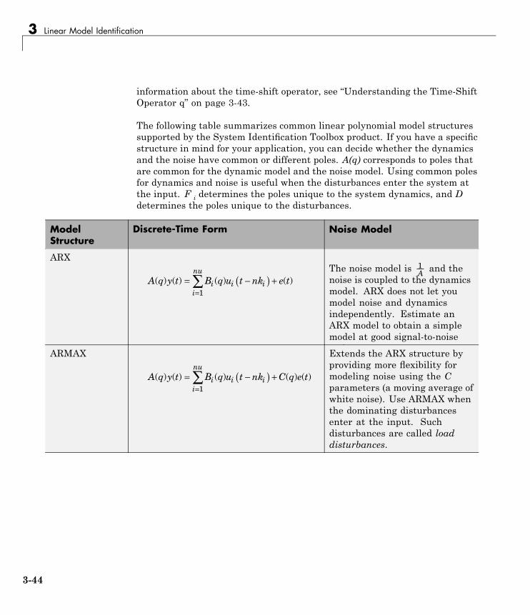
3 Linear Model Identification
information about the time-shift operator, see “Understanding the Time-ShiftOperator q” on page 3-43.
The following table summarizes common linear polynomial model structuressupported by the System Identification Toolbox product. If you have a specificstructure in mind for your application, you can decide whether the dynamicsand the noise have common or different poles. A(q) corresponds to poles thatare common for the dynamic model and the noise model. Using common polesfor dynamics and noise is useful when the disturbances enter the system atthe input. F i determines the poles unique to the system dynamics, and Ddetermines the poles unique to the disturbances.
ModelStructure
Discrete-Time Form Noise Model
ARX
A q y t B q u t nk e ti i ii
nu( ) ( ) ( ) ( )= −( ) +
=∑
1
The noise model is 1A and the
noise is coupled to the dynamicsmodel. ARX does not let youmodel noise and dynamicsindependently. Estimate anARX model to obtain a simplemodel at good signal-to-noiseratios.ARMAX
A q y t B q u t nk C q e ti i ii
nu( ) ( ) ( ) ( ) ( )= −( ) +
=∑
1
Extends the ARX structure byproviding more flexibility formodeling noise using the Cparameters (a moving average ofwhite noise). Use ARMAX whenthe dominating disturbancesenter at the input. Suchdisturbances are called loaddisturbances.
3-44
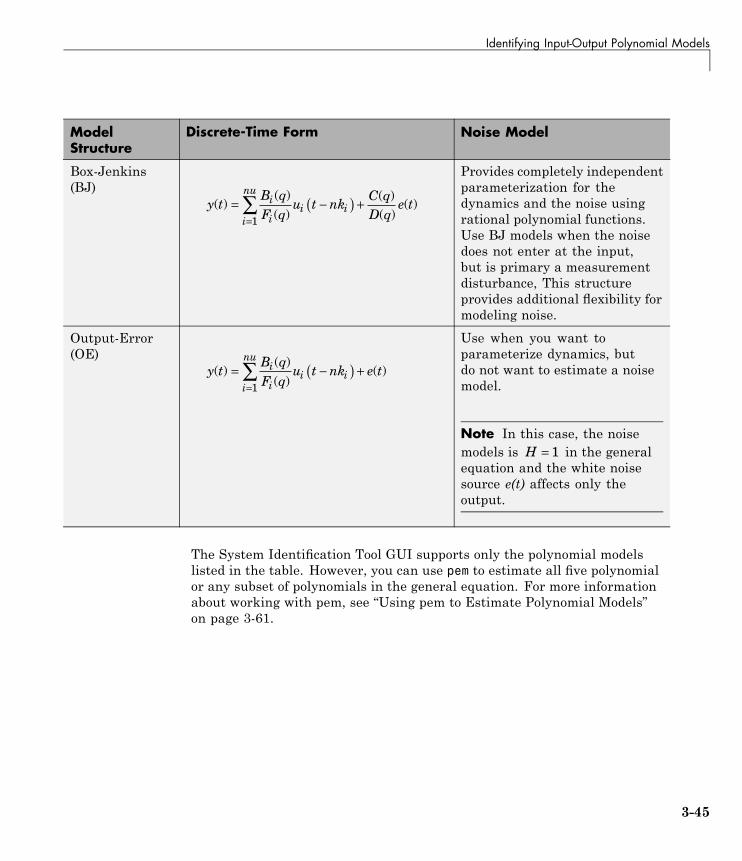
Identifying Input-Output Polynomial Models
ModelStructure
Discrete-Time Form Noise Model
Box-Jenkins(BJ)
y tB qF q
u t nkC qD q
e ti
ii i
i
nu( )
( )( )
( )( )
( )= −( ) +=∑
1
Provides completely independentparameterization for thedynamics and the noise usingrational polynomial functions.Use BJ models when the noisedoes not enter at the input,but is primary a measurementdisturbance, This structureprovides additional flexibility formodeling noise.
Output-Error(OE)
y tB qF q
u t nk e ti
ii i
i
nu( )
( )( )
( )= −( ) +=∑
1
Use when you want toparameterize dynamics, butdo not want to estimate a noisemodel.
Note In this case, the noisemodels is H = 1 in the generalequation and the white noisesource e(t) affects only theoutput.
The System Identification Tool GUI supports only the polynomial modelslisted in the table. However, you can use pem to estimate all five polynomialor any subset of polynomials in the general equation. For more informationabout working with pem, see “Using pem to Estimate Polynomial Models”on page 3-61.
3-45

3 Linear Model Identification
Definition of a Continuous-Time Polynomial ModelIn continuous time, the general frequency-domain equation is written in termsof the Laplace transform variable s, which corresponds to a differentiationoperation:
A s Y sB sF s
U sC sD s
E s( ) ( )( )( )
( )( )( )
( )= +
In the continuous-time case, the underlying time-domain model is adifferential equation and the model order integers represent the number ofestimated numerator and denominator coefficients. For example, na=3 andnb=2 correspond to the following model:
A s s a s a s a
B s b s b
( )( )
= + + += +
41
32
23
1 2
The simplest way to estimate continuous-time polynomial models ofarbitrary structure is to first estimate a discrete-time model of arbitraryorder and then use d2c to convert this model to continuous time. For moreinformation, see “Transforming Between Discrete-Time and Continuous-TimeRepresentations” on page 3-112.
You can also estimate continuous-time polynomial models directly usingcontinuous-time frequency-domain data. In this case, you must set the Ts dataproperty to 0 to indicate that you have continuous-time frequency-domaindata.
Definition of Multiple-Output ARX ModelsYou can use a multiple-output ARX model to model a multiple-output dynamicsystem. The ARX model structure is given by the following equation:
A q y t B q u t nk e t( ) ( ) ( ) ( )= −( ) +
3-46

Identifying Input-Output Polynomial Models
For a system with nu inputs and ny outputs, A(q) is an ny-by-ny matrix. A(q)can be represented as a polynomial in the shift operator q-1:
A q I A q A qny nana( ) = + + +− −
11 …
For more information about the time-shift operator, see “Understanding theTime-Shift Operator q” on page 3-43.
A(q) can also be represented as a matrix:
A q
a q a q a qa q a q a q
a q a
ny
ny
ny n
( )
( ) ( ) ( )( ) ( ) ( )
( )
=
11 12 1
21 22 2
1
……
… … … …
yy nyny qq a2( ) ( )…
⎛
⎝
⎜⎜⎜⎜⎜
⎞
⎠
⎟⎟⎟⎟⎟
where the matrix element akj is a polynomial in the shift operator q-1:
a q a q a qkj kj kj kjna nakj kj( ) = + + +− −δ 1 1 …
δkj represents the Kronecker delta, which equals 1 for k=j and equals 0for k≠j. This polynomial describes how the old values of the jth output areaffected by the kth output. The ith row of A(q) represents the contribution ofthe past output values for predict the current value of the ith output.
B(q) is an ny-by-ny matrix. B(q) can be represented as a polynomial in theshift operator q-1:
B q B B q B qnbnb( ) = + + +− −
0 11 …
3-47

3 Linear Model Identification
B(q) can also be represented as a matrix:
B q
b q b q b qb q b q b q
b q b
nu
nu
ny n
( )
( ) ( ) ( )( ) ( ) ( )
( )
=
11 12 1
21 22 2
1
……
… … … …
yy nynu qq b2( ) ( )…
⎛
⎝
⎜⎜⎜⎜⎜
⎞
⎠
⎟⎟⎟⎟⎟
where the matrix element bkj is a polynomial in the shift operator q-1:
b q a q a qkj kjnb
kjnk nb nbkj kj kj kj( ) = + +− − − +1 1…
nkkj is the delay from the jth input to the kth output. B(q) represents thecontributions of inputs to predicting all output values.
Data Supported by Polynomial Models
• “Types of Supported Data” on page 3-48
• “Designating Data for Estimating Continuous-Time Models” on page 3-49
• “Designating Data for Estimating Discrete-Time Models” on page 3-49
Types of Supported DataYou can estimate linear, black-box polynomial models from data with thefollowing characteristics:
• Time- or frequency-domain data (iddata or idfrd data objects).
Note For frequency-domain data, you can only estimate ARX and OEmodels.
To estimate black-box polynomial models for time-series data, see Chapter6, “Time Series Model Identification”.
• Real data or complex data in any domain.
3-48

Identifying Input-Output Polynomial Models
• Single-output and multiple-output.
You must import your data into the MATLAB workspace, as described inChapter 1, “Data Processing”.
Designating Data for Estimating Continuous-Time ModelsTo get a linear, continuous-time model of arbitrary structure for time-domaindata, you can estimate a discrete-time model, and then use d2c to transformit to a continuous-time model.
For continuous-time frequency-domain data, you can estimate directly onlythe ARX and Output-Error (OE) continuous-time models. Other structuresinclude noise models, which is not supported for frequency-domain data.
Tip To denote continuous-time frequency-domain data, set the data samplinginterval to 0. You can set the sampling interval when you import data intothe GUI or set the Ts property of the data object at the command line.
Designating Data for Estimating Discrete-Time ModelsYou can estimate arbitrary-order, linear state-space models for both time- orfrequency-domain data.
Your data must have the data property Ts set to the experimental datasampling interval.
Tip You can set the sampling interval when you import data into the GUI orset the Ts property of the data object at the command line.
Preliminary Step – Estimating Model Orders andInput Delays
• “Why Estimate Model Orders and Delays?” on page 3-50
• “Estimating Orders and Delays in the GUI” on page 3-50
3-49

3 Linear Model Identification
• “Estimating Model Orders at the Command Line” on page 3-53
• “Estimating Delays at the Command Line” on page 3-55
• “Selecting Model Orders from the Best ARX Structure” on page 3-55
Why Estimate Model Orders and Delays?To estimate polynomial models, you must provide input delays and modelorders. If you already have insight into the physics of your system, you canspecify the number of poles and zeros.
In most cases, you do not know the model orders in advance. To get initialmodel orders and delays for your system, you can estimate several ARXmodels with a range of orders and delays and compare the performance ofthese models. You choose the model orders that correspond to the best modelperformance and use these orders as an initial guess for further modeling.
Because this estimation procedure uses the ARX model structure, whichincludes the A and B polynomials, you only get estimates for the na, nb, andnk parameters. However, you can use these results as initial guesses for thecorresponding polynomial orders and input delays in other model structures,such as ARMAX, OE, and BJ.
If the estimated nk is too small, the leading nb coefficients are much smallerthan their standard deviations. Conversely, if the estimated nk is too large,there is a significant correlation between the residuals and the input for lagsthat correspond to the missing B terms. For information about residualanalysis plots, see “Using Residual Analysis Plots to Validate Models” onpage 8-16.
Estimating Orders and Delays in the GUIThe following procedure assumes that you have already imported your datainto the GUI and performed any necessary preprocessing operations. Formore information, see Chapter 1, “Data Processing”.
To estimate model orders and input delays in the System Identification ToolGUI:
3-50
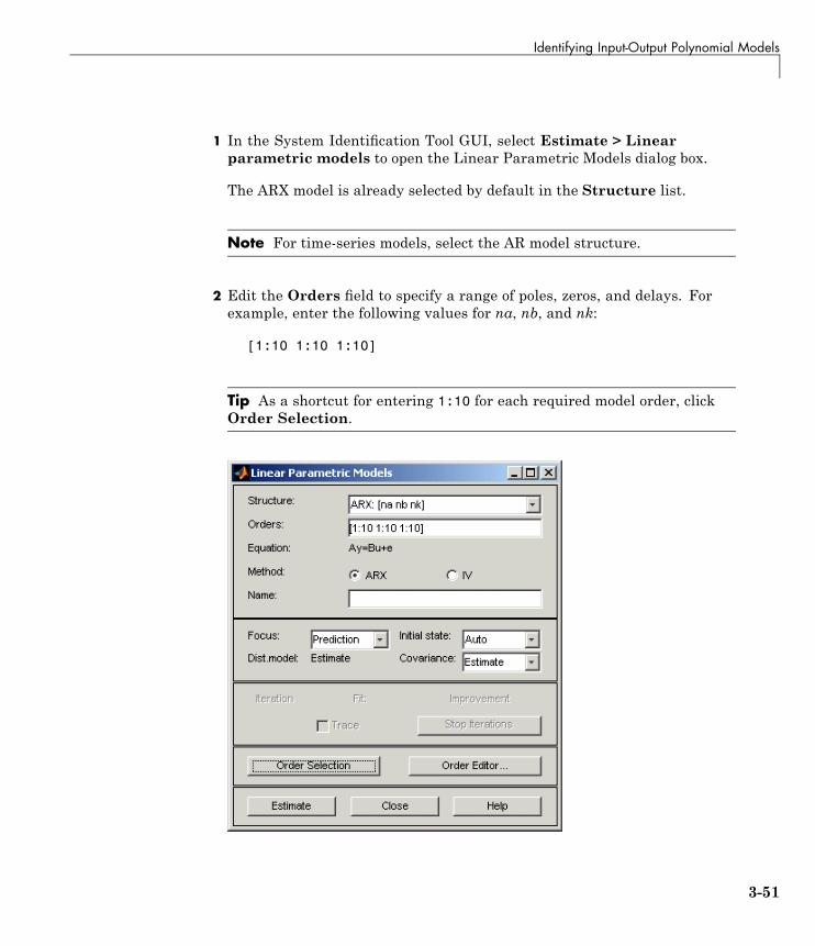
Identifying Input-Output Polynomial Models
1 In the System Identification Tool GUI, select Estimate > Linearparametric models to open the Linear Parametric Models dialog box.
The ARX model is already selected by default in the Structure list.
Note For time-series models, select the AR model structure.
2 Edit the Orders field to specify a range of poles, zeros, and delays. Forexample, enter the following values for na, nb, and nk:
[1:10 1:10 1:10]
Tip As a shortcut for entering 1:10 for each required model order, clickOrder Selection.
3-51
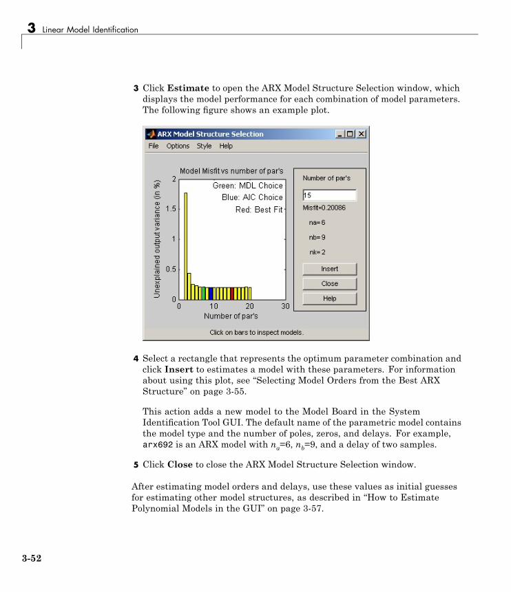
3 Linear Model Identification
3 Click Estimate to open the ARX Model Structure Selection window, whichdisplays the model performance for each combination of model parameters.The following figure shows an example plot.
4 Select a rectangle that represents the optimum parameter combination andclick Insert to estimates a model with these parameters. For informationabout using this plot, see “Selecting Model Orders from the Best ARXStructure” on page 3-55.
This action adds a new model to the Model Board in the SystemIdentification Tool GUI. The default name of the parametric model containsthe model type and the number of poles, zeros, and delays. For example,arx692 is an ARX model with na=6, nb=9, and a delay of two samples.
5 Click Close to close the ARX Model Structure Selection window.
After estimating model orders and delays, use these values as initial guessesfor estimating other model structures, as described in “How to EstimatePolynomial Models in the GUI” on page 3-57.
3-52
Identifying Input-Output Polynomial Models
Estimating Model Orders at the Command LineYou can estimate model orders using the struc, arxstruc, and selstruccommands in combination.
If you are working with a multiple-output system, you must use struc,arxstruc, and selstruc commands for each output. In this case, you mustsubreference the correct output channel in your estimation and validationdata sets.
For each estimation, you use two independent data sets—an estimation dataset and a validation data set. These independent data set can be from differentexperiments, or you can select these data sets from a single experiment. Formore information about subreferencing data, see “Subreferencing iddataObjects” on page 1-55 and “Subreferencing idfrd Objects” on page 1-70.
For an example of estimating model orders for a multiple-input system, see“Estimating Delays in the Multiple-Input System” in System IdentificationToolbox Getting Started Guide.
struc. The struc command creates a matrix of possible model-ordercombinations for a specified range of na, nb, and nk values.
For example, the following command defines the range of model orders anddelays na=2:5, nb=1:5, and nk=1:5:
NN = struc(2:5,1:5,1:5))
Note struc applies only to single-input/single-output models. If youhave multiple inputs and want to use struc, apply this command to oneinput-output pair at a time.
arxstruc. The arxstruc command takes the output from struc, estimatesan ARX model for each model order, and compares the model output to themeasured output. arxstruc returns the loss for each model, which is thenormalized sum of squared prediction errors.
3-53

3 Linear Model Identification
For example, the following command uses the range of specified orders NNto compute the loss function for single-input/single-output estimation datadata_e and validation data data_v:
V = arxstruc(data_e,data_v,NN)
Each row in NN corresponds to one set of orders:
[na nb nk]
selstruc. The selstruc command takes the output from arxstruc and opensthe ARX Model Structure Selection window to guide your choice of the modelorder with the best performance.
For example, to open the ARX Model Structure Selection window andinteractively choose the optimum parameter combination, use the followingcommand:
selstruc(V)
For more information about working with the ARX Model Structure Selectionwindow, see “Selecting Model Orders from the Best ARX Structure” on page3-55.
To find the structure that minimizes Akaike’s Information Criterion, usethe following command:
nn = selstruc(V,'AIC')
where nn contains the corresponding na, nb, and nk orders.
Similarly, to find the structure that minimizes the Rissanen’s MinimumDescription Length (MDL), use the following command:
nn = selstruc(V,'MDL')
To select the structure with the smallest loss function, use the followingcommand:
nn = selstruc(V,0)
3-54

Identifying Input-Output Polynomial Models
After estimating model orders and delays, use these values as initial guessesfor estimating other model structures, as described in “Using pem to EstimatePolynomial Models” on page 3-61.
Estimating Delays at the Command LineThe delayest command estimates the time delay in a dynamic system byestimating a low-order, discrete-time ARX model and treating the delay as anunknown parameter.
By default, delayest assumes that na=nb=2 and that there is a goodsignal-to-noise ratio, and uses this information to estimate nk.
To estimate the delay for a data set data, type the following at the prompt:
delayest(data)
If your data has a single input, MATLAB computes a scalar value for theinput delay—equal to the number of data samples. If your data has multipleinputs, MATLAB returns a vector, where each value is the delay for thecorresponding input signal.
To compute the actual delay time, you must multiply the input delay by thesampling interval of the data.
You can also use the ARX Model Structure Selection window to estimate inputdelays and model order together, as described in “Estimating Model Orders atthe Command Line” on page 3-53.
Selecting Model Orders from the Best ARX StructureYou generate the ARX Model Structure Selection window for your data toselect the best-fit model.
For a procedure on generating this plot in the System Identification Tool GUI,see “Estimating Orders and Delays in the GUI” on page 3-50. To open thisplot at the command line, see “Estimating Model Orders at the CommandLine” on page 3-53.
The following figure shows a sample plot in the ARX Model StructureSelection window.
3-55

3 Linear Model Identification
The horizontal axis in the ARX Model Structure Selection window is the totalnumber of ARX parameters:
Number of parameters = +n na b
The vertical axis, called Unexplained output variance (in %), is the ARXmodel prediction error for a specific number of parameters. The predictionerror is the sum of the squares of the differences between the validationdata output and the model output. In other words, Unexplained outputvariance (in %) is the portion of the output not explained by the model.
Three rectangles are highlighted on the plot—green, blue, and red. Each colorindicates a type of best-fit criterion, as follows:
• Red minimizes the sum of the squares of the difference between thevalidation data output and the model output. This option is considered theoverall best fit.
• Green minimizes Rissanen MDL criterion.
3-56
Identifying Input-Output Polynomial Models
• Blue minimizes Akaike AIC criterion.
In the ARX Model Structure Selection window, click any bar to view theorders that give the best fit. The area on the right is dynamically updated toshow the orders and delays that give the best fit.
For more information about the AIC criterion, see “Using Akaike’s Criteria toValidate Models” on page 8-61.
How to Estimate Polynomial Models in the GUI
• “Before You Begin” on page 3-57
• “Estimating Polynomial Models in the GUI” on page 3-57
Before You BeginBefore you estimate polynomial models, you must have already imported yourdata into the GUI and performed any necessary preprocessing operations. Formore information, see Chapter 1, “Data Processing”.
This procedure also requires that you select a model structure and specifymodel orders and delays. For more information about how to estimate modelorders and delays, see “Estimating Orders and Delays in the GUI” on page3-50.
If you are estimating a multiple-output ARX model, you must specify ordermatrices in the MATLAB workspace before estimation, as described in“Options for Multiple-Input and Multiple-Output ARX Orders” on page 3-64.
Estimating Polynomial Models in the GUITo estimate a polynomial model in the System Identification Tool GUI.
1 In the System Identification Tool GUI, select Estimate > Linearparametric models to open the Linear Parametric Models dialog box.
3-57

3 Linear Model Identification
2 In the Structure list, select the polynomial model structure you want toestimate from the following options:
• ARX:[na nb nk]
• ARMAX:[na nb nc nk]
• OE:[nb nf nk]
• BJ:[nb nc nd nf nk]
This action updates the options in the Linear Parametric Models dialog boxto correspond with this model structure. For information about each modelstructure, see “What Are Black-Box Polynomial Models?” on page 3-41.
Note For time-series data, only AR and ARMA models are available. Formore information about estimating time-series models, see Chapter 6,“Time Series Model Identification”.
3 In the Orders field, specify the model orders and delays, as follows:
• For single-output polynomial models. Enter the model orders anddelays according to the sequence displayed in the Structure field. Formultiple-input models, specify nb and nk as row vectors with as manyelements as there are inputs. If you are estimating BJ and OE models,you must also specify nf as a vector.
For example, for a three-input system, nb can be [1 2 4], where eachelement corresponds to an input.
• For multiple-output ARX models. Enter the model orders, asdescribed in “Options for Multiple-Input and Multiple-Output ARXOrders” on page 3-64.
Tip To enter model orders and delays using the Order Editor dialog box,click Order Editor.
4 (ARX models only) Select the estimation Method as ARX or IV(instrumental variable method). For information about the algorithms, see“Algorithms for Estimating Polynomial Models” on page 3-66.
3-58

Identifying Input-Output Polynomial Models
5 In the Name field, edit the name of the model or keep the default. Thename of the model should be unique in the Model Board.
6 In the Focus list, select how to weigh the relative importance of the fit atdifferent frequencies. For more information about each option, see “Optionfor Frequency-Weighing Focus” on page 3-65.
7 In the Initial state list, specify how you want the algorithm to treat initialstates. For more information about the available options, see “Options forInitial States” on page 3-39.
Tip If you get an inaccurate fit, try setting a specific method for handlinginitial states rather than choosing it automatically.
8 In the Covariance list, select Estimate if you want the algorithm tocompute parameter uncertainties. Effects of such uncertainties aredisplayed on plots as model confidence regions.
To omit estimating uncertainty, select None. Skipping uncertaintycomputation for large, multiple-output ARX models might reducecomputation time.
9 (ARMAX, OE, and BJ models only) To view the estimation progress inthe MATLAB Command Window, select the Trace check box. Duringestimation, the following information is displayed for each iteration:
• Loss function — Equals the determinant of the estimated covariancematrix of the input noise.
• Parameter values — Values of the model structure coefficients youspecified.
• Search direction — Change in parameter values from the previousiteration.
• Fit improvements — Shows the actual versus expected improvements inthe fit.
10 Click Estimate to add this model to the Model Board in the SystemIdentification Tool GUI.
3-59
3 Linear Model Identification
11 (Prediction-error method only) To stop the search and save the resultsafter the current iteration has been completed, click Stop Iterations. Tocontinue iterations from the current model, click the Continue iter buttonto assign current parameter values as initial guesses for the next search.
12 To plot the model, select the appropriate check box in the Model Viewsarea of the System Identification Tool GUI. For more information aboutvalidating models, see “Overview of Model Validation and Plots” on page8-2.
If you get an inaccurate fit, try estimating a new model with different ordersor structure. You can export the model to the MATLAB workspace for furtheranalysis by dragging it to the To Workspace rectangle in the SystemIdentification Tool GUI.
How to Estimate Polynomial Models at the CommandLine
• “Using arx and iv4 to Estimate ARX Models” on page 3-60
• “Using pem to Estimate Polynomial Models” on page 3-61
Using arx and iv4 to Estimate ARX ModelsYou can estimate single-output and multiple-output ARX models usingthe arx and iv4 commands. For information about the algorithms, see“Algorithms for Estimating Polynomial Models” on page 3-66.
If you are estimating a multiple-output ARX model, you must specify ordermatrices in the MATLAB workspace before estimation, as described in“Options for Multiple-Input and Multiple-Output ARX Orders” on page 3-64.
For single-output data, the arx and iv4 commands produce an idpoly modelobject, and for multiple-output data these commands produce an idarx modelobject.
You can use the following general syntax to both configure and estimate ARXmodels:
% Using ARX method
3-60
Identifying Input-Output Polynomial Models
m = arx(data,[na nb nk],'Property1',Value1,...,'PropertyN',ValueN)
% Using IV methodm = iv4(data,[na nb nk],'Property1',Value1,...,
'PropertyN',ValueN)
data is the estimation data and [na nb nk] specifies the model orders, asdiscussed in “What Are Black-Box Polynomial Models?” on page 3-41.
The property-value pairs specify any model properties that configure theestimation algorithm and the initial conditions. For more information aboutaccessing and setting model properties, see “Model Properties” on page 2-14.
Note You can specify all property-value pairs as a comma-separated list.
To get discrete-time models, use the time-domain data (iddata object). To geta single-output continuous-time model, apply d2c to a discrete-time modelor use continuous-time frequency-domain data—either idfrd object, orfrequency-domain iddata with Ts=0.
Note The System Identification Toolbox product does not supportmultiple-output continuous-time idarx models.
For more information about validating you model, see “Overview of ModelValidation and Plots” on page 8-2.
You can use pem to refine parameter estimates of an existing polynomialmodel, as described in “Refining Linear Parametric Models” on page 3-103.
For detailed information about these commands, see the correspondingreference page.
Using pem to Estimate Polynomial ModelsYou can estimate any single-output polynomial model using the iterativeprediction-error estimation method pem. For Gaussian disturbances, this
3-61

3 Linear Model Identification
method gives the maximum likelihood estimate. that minimizes the predictionerrors to obtain maximum-likelihood values. The resulting models are storedas idpoly model objects.
Use the following general syntax to both configure and estimate polynomialmodels:
m = pem(data,'na',na,'nb',nb,'nc',nc,'nd',nb,'nf',nc,'nk',nk,'Property1',Value1,...,'PropertyN',ValueN)
where data is the estimation data. na, nb, nc, nd, nf are integers that specifythe model orders, and nk specifies the input delays for each input. If youskip any property-value pair, the corresponding parameter value is set tozero—except nk, which has the default value 1. For more information aboutmodel orders, see “What Are Black-Box Polynomial Models?” on page 3-41.
Tip You do not need to construct the model object using idoly beforeestimation.
If you want to estimate the coefficients of all five polynomials, A, B, C, D, andF, you must specify an integer order for each polynomial. However, if youwant to specify an ARMAX model for example, which includes only the A, B,and C polynomials, you must set nd and nf to 0.
Note To get faster estimation of ARX models, use arx or iv4 instead of pem.
In addition to the polynomial models listed in “What Are Black-BoxPolynomial Models?” on page 3-41, you can use pem to model the ARARXstructure—called the generalized least-squares model—by setting nc=nf=0.
3-62

Identifying Input-Output Polynomial Models
You can also model the ARARMAX structure—called the extended matrixmodel—by setting nf=0.
The property-value pairs specify any model properties that configurethe estimation algorithm and the initial conditions. You can enter allproperty-value pairs in pem as a comma-separated list without worryingabout the hierarchy of these properties in the idpoly model object. Formore information about accessing and setting model properties, see “ModelProperties” on page 2-14.
For multiple inputs, nb, nf, and nk are row vectors of the same lengths as thenumber of input channels:
nb = [nb1 ... nbnu];nf = [nf1 ... nfnu];nk = [nk1 ... nknu];
For ARMAX, Box-Jenkins, and Output-Error models—which can only beestimated using the iterative prediction-error method—use the armax, bj, andoe estimation commands, respectively. These commands are versions of pemwith simplified syntax for these specific model structures, as follows:
m = armax(Data,[na nb nc nk])m = oe(Data,[nb nf nk])m = bj(Data,[nb nc nd nf nk])
Tip If your data is sampled fast, it might help to apply a lowpass filter to thedata before estimating the model. For example, to model only data in thefrequency range 0-10 rad/s, use the Focus property, as follows:
m = oe(Data,[nb nf nk],'Focus',[0 10])
For more information about validating you model, see “Overview of ModelValidation and Plots” on page 8-2.
You can use pem to refine parameter estimates of an existing polynomialmodel, as described in “Refining Linear Parametric Models” on page 3-103.
3-63
3 Linear Model Identification
For detailed information about pem and idpoly, see the correspondingreference page.
Options for Multiple-Input and Multiple-Output ARXOrdersTo estimate a multiple-input and multiple-output (MIMO) ARX model, youmust first specify the model order matrices, as follows:
• NA — An ny-by-ny matrix whose i-jth entry is the order of the polynomialthat relates the jth output to the ith output.
• NB — An ny-by-nu matrix whose i-jth entry is the order of the polynomialthat relates the jth input to the ith output.
• NK— An ny-by-nu matrix whose i-jth entry is the delay from the jth inputto the ith output.
• For ny outputs and nu inputs, the A coefficients are ny-by-ny matrices andthe B coefficients are ny-by-nu matrices. For more information aboutMIMO ARX structure, see “Definition of Multiple-Output ARX Models”on page 3-46.
Note For multiple-output time-series models, only AR models are supported.AR models require only the NA matrix.
In the System Identification Tool GUI. You can enter the matrices directlyin the Orders field.
At the command line. Define variables that store the model order matricesand specify these variables in the model-estimation command. You can usethe following syntax to estimate a model with these orders:
arx(data,'na',NA,'nb',NB,'nk',NK)
Tip To simplify entering large matrices orders in the System IdentificationTool GUI, define the variable NN=[NA NB NK] at the command line. You canspecify this variable in the Orders field.
3-64

Identifying Input-Output Polynomial Models
Option for Frequency-Weighing FocusYou can specify how the estimation algorithm weighs the fit at variousfrequencies. This information supports the estimation procedures “How toEstimate Polynomial Models in the GUI” on page 3-57 and “Using pem toEstimate Polynomial Models” on page 3-61.
In the System Identification Tool GUI. Set Focus to one of the followingoptions:
• Prediction— Uses the inverse of the noise model H to weigh the relativeimportance of how closely to fit the data in various frequency ranges.Corresponds to minimizing one-step-ahead prediction, which typicallyfavors the fit over a short time interval. Optimized for output predictionapplications.
• Simulation— Uses the input spectrum to weigh the relative importance ofthe fit in a specific frequency range. Does not use the noise model to weighthe relative importance of how closely to fit the data in various frequencyranges. Optimized for output simulation applications.
• Stability— Estimates the best stable model. For more information aboutmodel stability, see “Unstable Models” on page 8-69.
• Filter— Specify a custom filter to open the Estimation Focus dialog box,where you can enter a filter, as described in “Simple Passband Filter” onpage 1-111 or “Defining a Custom Filter” on page 1-112. This prefilteringapplies only for estimating the dynamics from input to output. Thedisturbance model is determined from the unfiltered estimation data.
At the command line. Specify the focus as an argument in themodel-estimation command using the same options as in the GUI. Forexample, use this command to estimate an ARX model and emphasize thefrequency content related to the input spectrum only:
m=arx(data,[2 2 3],'Focus','Simulation')
This Focus setting might produce more accurate simulation results.
3-65

3 Linear Model Identification
Options for Initial StatesWhen you use the iterative estimation algorithm PEM to estimate ARMAX,Box-Jenkins (BJ), Output-Error (OE), you must specify how the algorithmtreats initial states.
This information supports the estimation procedures “How to EstimatePolynomial Models in the GUI” on page 3-57 and “Using pem to EstimatePolynomial Models” on page 3-61.
In the System Identification Tool GUI. For ARMAX, OE, and BJ models,set Initial state to one of the following options:
• Auto— Automatically chooses Zero, Estimate, or Backcast based on theestimation data. If initial states have negligible effect on the predictionerrors, the initial states are set to zero to optimize algorithm performance.
• Zero — Sets all initial states to zero.
• Estimate— Treats the initial states as an unknown vector of parametersand estimates these states from the data.
• Backcast— Estimates initial states using a smoothing filter.
At the command line. Specify the initial states as an argument in themodel-estimation command. For example, use this command to estimate anARMAX model and set the initial states to zero:
m=armax(data,[2 2 2 3],'InitialState','zero')
For a complete list of values for the InitialState model property, see theidpoly reference page.
Algorithms for Estimating Polynomial ModelsFor linear ARX and AR models, you can choose between the ARX and IValgorithms. ARX implements the least-squares estimation method that usesQR-factorization for overdetermined linear equations. IV is the instrumentalvariable method. For more information about IV, see the section onvariance-optimal instruments in System Identification: Theory for the User,Second Edition, by Lennart Ljung, Prentice Hall PTR, 1999.
3-66

Identifying Input-Output Polynomial Models
The ARX and IV algorithms treat noise differently. ARX assumes white noise.However, the instrumental variable algorithm, IV, is not sensitive to noisecolor. Thus, use IV when the noise in your system is not completely white andit is incorrect to assume white noise. If the models you obtained using ARXare inaccurate, try using IV.
Note AR models apply to time-series data, which has no input. For moreinformation, see Chapter 6, “Time Series Model Identification”. For moreinformation about working with AR and ARX models, see “IdentifyingInput-Output Polynomial Models” on page 3-41.
Example – Estimating Models Using armaxYou can use estimation commands to both construct a model object andestimate the model parameters. In this example, you estimate a linear,polynomial model with an ARMAX structure for a three-input andsingle-output (MISO) system using the iterative estimation method armax.For a summary of all available estimation commands in the toolbox, see“Commands for Model Estimation” on page 2-9.
1 Load a sample data set z8 with three inputs and one output, measured at1-second intervals and containing 500 data samples:
load iddata8
2 Use armax to both construct the idpoly model object, and estimate theparameters:
A q y t B q u t nk C q e ti i ii
nu( ) ( ) ( ) ( ) ( )= −( ) +
=∑
1
3-67

3 Linear Model Identification
Typically you try different model orders and compare results, ultimatelychoosing the simplest model that best describes the system dynamics. Thefollowing command specifies the estimation data set, z8, and the orders ofthe A, B, and C polynomials as na, nb, and nc, respectively. nk of [0 0 0]specifies that there is no input delay for all three input channels.
m_armax=armax(z8,'na',4,...'nb',[3 2 3],...'nc',4,...'nk',[0 0 0],...'focus', 'simulation',...'tolerance',1e-5,...'maxiter',50);
covariance, focus, tolerance, and maxiter are optional argumentsspecify additional information about the computation. focus specifieswhether the model is optimized for simulation or prediction applications,tolerance and maxiter specify when to stop estimation. For moreinformation about these properties, see the algorithm propertiesreference page.
armax is a version of pem with simplified syntax for the ARMAX modelstructure. The armax method both constructs the idpoly model objectand estimates its parameters.
Tip Instead of specifying model orders and delays as individualproperty-value pairs, you can use the equivalent shorthand notation thatincludes all of the order integers in a single vector, as follows:
m_armax=armax(z8,[4 3 2 3 4 0 0 0],...'focus', 'simulation',...'tolerance',1e-5,...'maxiter',50);
3-68
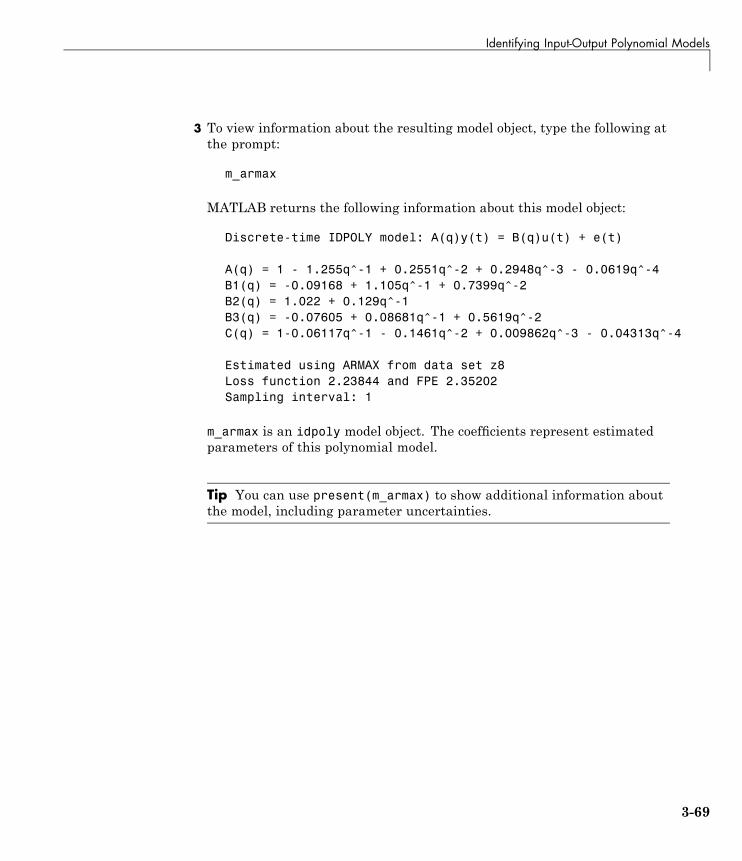
Identifying Input-Output Polynomial Models
3 To view information about the resulting model object, type the following atthe prompt:
m_armax
MATLAB returns the following information about this model object:
Discrete-time IDPOLY model: A(q)y(t) = B(q)u(t) + e(t)
A(q) = 1 - 1.255q^-1 + 0.2551q^-2 + 0.2948q^-3 - 0.0619q^-4B1(q) = -0.09168 + 1.105q^-1 + 0.7399q^-2B2(q) = 1.022 + 0.129q^-1B3(q) = -0.07605 + 0.08681q^-1 + 0.5619q^-2C(q) = 1-0.06117q^-1 - 0.1461q^-2 + 0.009862q^-3 - 0.04313q^-4
Estimated using ARMAX from data set z8Loss function 2.23844 and FPE 2.35202Sampling interval: 1
m_armax is an idpoly model object. The coefficients represent estimatedparameters of this polynomial model.
Tip You can use present(m_armax) to show additional information aboutthe model, including parameter uncertainties.
3-69
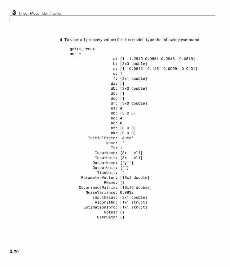
3 Linear Model Identification
4 To view all property values for this model, type the following command:
get(m_armaxans =
a: [1 -1.2549 0.2551 0.2948 -0.0619]b: [3x3 double]c: [1 -0.0612 -0.1461 0.0099 -0.0431]d: 1f: [3x1 double]
da: []db: [3x0 double]dc: []dd: []df: [3x0 double]na: 4nb: [3 2 3]nc: 4nd: 0nf: [0 0 0]nk: [0 0 0]
InitialState: 'Auto'Name: ''
Ts: 1InputName: {3x1 cell}InputUnit: {3x1 cell}
OutputName: {'y1'}OutputUnit: {''}
TimeUnit: ''ParameterVector: [16x1 double]
PName: {}CovarianceMatrix: [16x16 double]
NoiseVariance: 0.9932InputDelay: [3x1 double]Algorithm: [1x1 struct]
EstimationInfo: [1x1 struct]Notes: {}
UserData: []
3-70
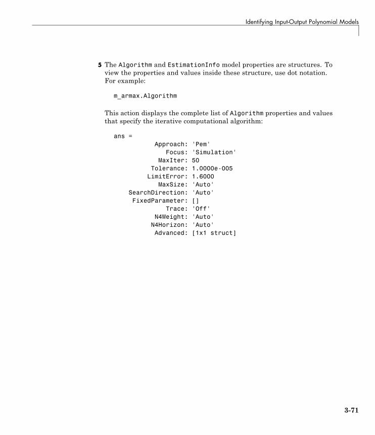
Identifying Input-Output Polynomial Models
5 The Algorithm and EstimationInfo model properties are structures. Toview the properties and values inside these structure, use dot notation.For example:
m_armax.Algorithm
This action displays the complete list of Algorithm properties and valuesthat specify the iterative computational algorithm:
ans =Approach: 'Pem'
Focus: 'Simulation'MaxIter: 50
Tolerance: 1.0000e-005LimitError: 1.6000
MaxSize: 'Auto'SearchDirection: 'Auto'FixedParameter: []
Trace: 'Off'N4Weight: 'Auto'
N4Horizon: 'Auto'Advanced: [1x1 struct]
3-71
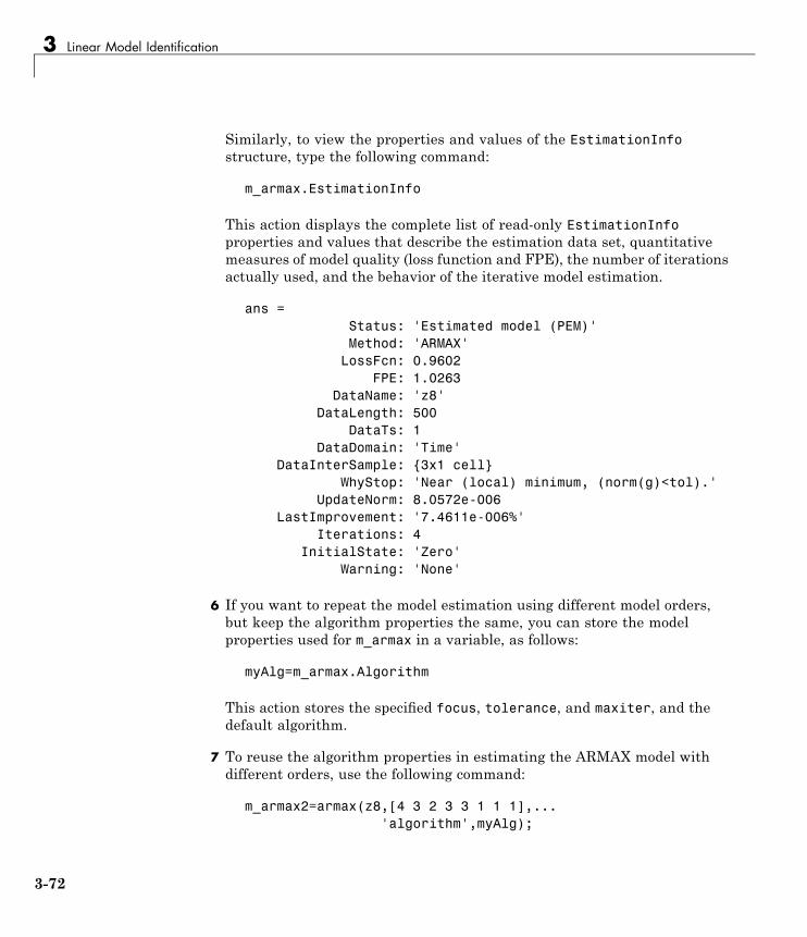
3 Linear Model Identification
Similarly, to view the properties and values of the EstimationInfostructure, type the following command:
m_armax.EstimationInfo
This action displays the complete list of read-only EstimationInfoproperties and values that describe the estimation data set, quantitativemeasures of model quality (loss function and FPE), the number of iterationsactually used, and the behavior of the iterative model estimation.
ans =Status: 'Estimated model (PEM)'Method: 'ARMAX'
LossFcn: 0.9602FPE: 1.0263
DataName: 'z8'DataLength: 500
DataTs: 1DataDomain: 'Time'
DataInterSample: {3x1 cell}WhyStop: 'Near (local) minimum, (norm(g)<tol).'
UpdateNorm: 8.0572e-006LastImprovement: '7.4611e-006%'
Iterations: 4InitialState: 'Zero'
Warning: 'None'
6 If you want to repeat the model estimation using different model orders,but keep the algorithm properties the same, you can store the modelproperties used for m_armax in a variable, as follows:
myAlg=m_armax.Algorithm
This action stores the specified focus, tolerance, and maxiter, and thedefault algorithm.
7 To reuse the algorithm properties in estimating the ARMAX model withdifferent orders, use the following command:
m_armax2=armax(z8,[4 3 2 3 3 1 1 1],...'algorithm',myAlg);
3-72

Identifying State-Space Models
Identifying State-Space Models
In this section...
“What Are State-Space Models?” on page 3-73“Data Supported by State-Space Models” on page 3-77“Supported State-Space Parameterizations” on page 3-78“Preliminary Step – Estimating State-Space Model Orders” on page 3-79“How to Estimate State-Space Models in the GUI” on page 3-84“How to Estimate State-Space Models at the Command Line” on page 3-87“How to Estimate Free-Parameterization State-Space Models” on page 3-90“How to Estimate State-Space Models with Canonical Parameterization”on page 3-91“How to Estimate State-Space Models with Structured Parameterization”on page 3-93“How to Estimate the State-Space Equivalent of ARMAX and OE Models”on page 3-100“Options for Frequency-Weighing Focus” on page 3-100“Options for Initial States” on page 3-101“Algorithms for Estimating State-Space Models” on page 3-101
What Are State-Space Models?
• “Definition of State-Space Models” on page 3-74
• “Continuous-Time Representation” on page 3-74
• “Discrete-Time Representation” on page 3-75
• “Relationship Between Continuous-Time and Discrete-Time StateMatrices” on page 3-75
• “State-Space Representation of Transfer Functions” on page 3-76
3-73

3 Linear Model Identification
Definition of State-Space ModelsState-space models are models that use state variables to describe a system bya set of first-order differential or difference equations, rather than by one ormore nth-order differential or difference equations. State variables x(t) can bereconstructed from the measured input-output data, but are not themselvesmeasured during an experiment.
The state-space model structure is a good choice for quick estimation becauseit requires only two parameters:
• n— Model order or the number of poles (size of the A matrix).
• nk — One or more input delays.
The model order for state-space models is an integer equal to the dimensionof x(t) and relates to the number of delayed inputs and outputs used in thecorresponding linear difference equation.
Continuous-Time RepresentationIn continuous-time, the state-space description has the following form:
� �x t Fx t Gu t Kw ty t Hx t Du t w tx x
( ) ( ) ( ) ( )( ) ( ) ( ) ( )( )
= + += + +=0 0
It is often easier to define a parameterized state-space model in continuoustime because physical laws are most often described in terms of differentialequations. In this case, the matrices F, G, H, and D contain elements withphysical significance—for example, material constants. x0 specifies the initialstates.
Note K=0 gives the state-space representation of an Output-Error model.For more information about Output-Error models, see “What Are Black-BoxPolynomial Models?” on page 3-41.
3-74

Identifying State-Space Models
Discrete-Time RepresentationDiscrete-time state-space models provide the same type of linear differencerelationship between the inputs and the outputs as the linear ARX model, butare rearranged such that there is only one delay in the expressions. Thediscrete-time state-space model structure is often written in the innovationsform that describes noise:
x kT T Ax kT Bu kT Ke kTy kT Cx kT Du kT e kTx
( ) ( ) ( ) ( )( ) ( ) ( ) ( )( )
+ = + += + +
=0 xx0
where T is the sampling interval, u(kT) is the input at time instant kT, andy(kT) is the output at time instant kT.
Note K=0 gives the state-space representation of an Output-Error model.For more information about Output-Error models, see “What Are Black-BoxPolynomial Models?” on page 3-41.
Relationship Between Continuous-Time and Discrete-TimeState MatricesThe relationships between the discrete state-space matrices A, B, C, D, and Kand the continuous-time state-space matrices F, G, H, D, and �K are given forpiece-wise-constant input, as follows:
A e
B e Gd
C H
FT
FT
=
=
=
∫ τ τ0
These relationships assume that the input is piece-wise-constant over timeintervals kT t k T≤ < +( )1 .
3-75

3 Linear Model Identification
The exact relationship between K and �K is complicated. However, for shortsampling intervals T, the following approximation works well:
K e KdFT
= ∫ τ τ�
0
State-Space Representation of Transfer FunctionsFor linear models, the general symbolic model description is given by:
y Gu He= +
G is a transfer function that takes the input u to the output y. H is a transferfunction that describes the properties of the additive output noise model.
The discrete-time state-space representation is given by the followingequation:
x kT T Ax kT Bu kT Ke kTy kT Cx kT Du kT e kTx
( ) ( ) ( ) ( )( ) ( ) ( ) ( )( )
+ = + += + +
=0 xx0
where T is the sampling interval, u(kT) is the input at time instant kT, andy(kT) is the output at time instant kT.
The relationships between the transfer functions and the discrete-timestate-space matrices are given by the following equations:
G q C qI A B D
H q C qI A K I
nx
nx ny
( ) ( )
( ) ( )
= − +
= − +
−
−
1
1
where Inx is the nx-by-nx identity matrix, Iny is the nx-by-nx identity matrix,and ny is the dimension of y and e.
3-76
Identifying State-Space Models
Data Supported by State-Space Models
• “Types of Supported Data” on page 3-77
• “Estimating Continuous-Time Models” on page 3-77
• “Designating Data for Estimating Discrete-Time Models” on page 3-78
Types of Supported DataYou can estimate linear state-space models from data with the followingcharacteristics:
• Real data or complex data in any domain
• Single-output and multiple-output
• Time- or frequency-domain data
To estimate state-space models for time-series data, see Chapter 6, “TimeSeries Model Identification”.
You must first import your data into the MATLAB workspace, as described inChapter 1, “Data Processing”.
Estimating Continuous-Time ModelsUse either of the following ways to estimate continuous-time, state-spacemodels:
• To get a linear, continuous-time model of arbitrary structure fortime-domain data, you can estimate a discrete-time model, and then used2c to transform it to a continuous-time model.
• Use continuous-time frequency-domain data.
To denote continuous-time frequency-domain data, set the data samplinginterval to 0. You can set the sampling interval when you import data intothe GUI or set the Ts property of the data object at the command line.
3-77
3 Linear Model Identification
Tip Continuous state-space models are available for canonical andstructured parameterizations and grey-box models. In this case, nodisturbance model can be estimated.
Designating Data for Estimating Discrete-Time ModelsYou can estimate arbitrary-order, linear state-space models for both time- orfrequency-domain data.
You must specify your data to have the sampling interval equal to theexperimental data sampling interval.
You can set the sampling interval when you import data into the GUI or setthe Ts property of the data object at the command line.
Supported State-Space ParameterizationsThe System Identification Toolbox product supports the followingparameterizations that indicate which parameters are estimated and whichremain fixed at specific values:
• Free parameterization results in the estimation of all system matrixelements A, B, C, D, and K.
• Canonical forms of A, B, C, D, and K matrices.
Canonical parameterization represents a state-space system in its minimalform, using the minimum number of free parameters to capture thedynamics. Thus, free parameters appear in only a few of the rows andcolumns in system matrices A, B, C, and D, and the remaining matrixelements are fixed to zeros and ones.
• Structured parameterization lets you specify the values of specificparameters and exclude these parameters from estimation.
• Completely arbitrary mapping of parameters to state-space matrices. Formore information, see “Estimating Linear Grey-Box Models” on page 5-6.
3-78

Identifying State-Space Models
You can only estimate free state-space models in discrete time.Continuous state-space models are available for canonical and structuredparameterizations and grey-box models.
Note To estimate canonical and structured state-space models in the SystemIdentification Tool GUI, define the corresponding model structures at thecommand line and import them into the System Identification Tool GUI.
Preliminary Step – Estimating State-Space ModelOrders
• “Why Estimate Model Orders?” on page 3-79
• “Estimating Model Order in the GUI” on page 3-79
• “Estimating the Model Order at the Command Line” on page 3-82
• “Using the Model Order Selection Window” on page 3-83
Why Estimate Model Orders?To estimate a state-space model, you must provide a model order and oneor more input delays.
To get an initial model order for your system, you can estimate a group ofstate-space models with a range of orders for a specific delay and compare theperformance of these models. You choose the model order that include stateswith the highest contribution to the input-output behavior of the model anduse this order as an initial guess for further modeling.
The model order is always a single integer—regardless of the number ofinputs and outputs. However, the number of input delays must correspond tothe number of input channels.
Estimating Model Order in the GUIYou must have already imported your data into the GUI, as described in“Representing Data in the GUI” on page 1-13.
3-79

3 Linear Model Identification
To estimate model orders for a specific input delay:
1 In the System Identification Tool GUI, select Estimate > Linearparametric models to open the Linear Parametric Models dialog box.
2 In the Structure list, select State Space: n [nk].
3 Edit the Orders field to specify a range of orders for a specific delay. Forexample, enter the following values for n and nk:
1:10 [1]
Tip As a shortcut for entering 1:10 [1], click Order Selection.
4 Verify that the Method is set to N4SID.
3-80
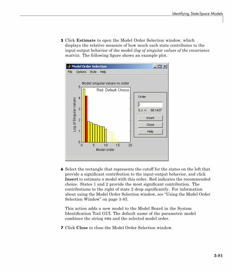
Identifying State-Space Models
5 Click Estimate to open the Model Order Selection window, whichdisplays the relative measure of how much each state contributes to theinput-output behavior of the model (log of singular values of the covariancematrix). The following figure shows an example plot.
6 Select the rectangle that represents the cutoff for the states on the left thatprovide a significant contribution to the input-output behavior, and clickInsert to estimate a model with this order. Red indicates the recommendedchoice. States 1 and 2 provide the most significant contribution. Thecontributions to the right of state 2 drop significantly. For informationabout using the Model Order Selection window, see “Using the Model OrderSelection Window” on page 3-83.
This action adds a new model to the Model Board in the SystemIdentification Tool GUI. The default name of the parametric modelcombines the string n4s and the selected model order.
7 Click Close to close the Model Order Selection window.
3-81
3 Linear Model Identification
After estimating model orders, use this value as an initial guess for estimatingother state-space models, as described in “How to Estimate State-SpaceModels in the GUI” on page 3-84.
Estimating the Model Order at the Command LineYou can estimate the state-space model order using the n4sid command.
Use following syntax to specify the range of model orders to try for a specificinput delay.
m = n4sid(data,n1:n2,'nk',nk);
where data is the estimation data set, n1 and n2 specify the range of orders,and nk specifies the input delay. For multiple-input systems, nk is a vectorof input delays.
This command opens the Model Order Selection window. For informationabout using this plot, see “Using the Model Order Selection Window” on page3-83.
Alternatively, you can use the pem command to open the Model OrderSelection window, as follows:
m = pem(Data,'nx',nn)
where nn = [n1,n2,...,nN] specifies the vector or range of orders youwant to try.
To omit opening the Model Order Selection window and automatically selectthe best order, use the following syntax:
m = pem(Data,'best')
For a tutorial on estimating model orders for a multiple-input system, see“Estimating a State-Space Model” in System Identification Toolbox GettingStarted Guide.
3-82
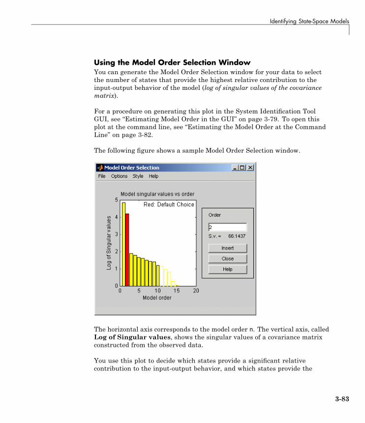
Identifying State-Space Models
Using the Model Order Selection WindowYou can generate the Model Order Selection window for your data to selectthe number of states that provide the highest relative contribution to theinput-output behavior of the model (log of singular values of the covariancematrix).
For a procedure on generating this plot in the System Identification ToolGUI, see “Estimating Model Order in the GUI” on page 3-79. To open thisplot at the command line, see “Estimating the Model Order at the CommandLine” on page 3-82.
The following figure shows a sample Model Order Selection window.
The horizontal axis corresponds to the model order n. The vertical axis, calledLog of Singular values, shows the singular values of a covariance matrixconstructed from the observed data.
You use this plot to decide which states provide a significant relativecontribution to the input-output behavior, and which states provide the
3-83
3 Linear Model Identification
smallest contribution. Based on this plot, select the rectangle that representsthe cutoff for the states on the left that provide a significant contribution tothe input-output behavior. The recommended choice is red.
For example, in the previous figure, states 1 and 2 provide the most significantcontribution. However, the contributions of the states to the right of state 2drop significantly. This sharp decrease in the log of the singular values aftern=2 indicates that using two states is sufficient to get an accurate model.
How to Estimate State-Space Models in the GUI
• “Supported State-Space Models in the GUI” on page 3-84
• “Before You Begin” on page 3-84
• “Estimating State-Space Models in the GUI” on page 3-84
Supported State-Space Models in the GUIOnly free parameterization is directly supported in the System IdentificationTool GUI. You can also estimate canonical and structured parameterizationsat the command line and import them into the System Identification ToolGUI for parameter estimation. For more information about state-spaceparameterization, see “Supported State-Space Parameterizations” on page3-78.
Before You BeginBefore you estimate state-space models, you must have already imported yourdata into the GUI and performed any necessary preprocessing operations. Formore information, see Chapter 1, “Data Processing”.
The following procedure also requires that you specify model order andinput delays. For more information about how to estimate model orders, see“Estimating Model Order in the GUI” on page 3-79.
Estimating State-Space Models in the GUITo estimate a state-space model with free parameterization in the SystemIdentification Tool GUI:
3-84
Identifying State-Space Models
1 In the System Identification Tool GUI, select Estimate > Linearparametric models to open the Linear Parametric Models dialog box.
2 In the Structure list, select State Space: n [nk].
This action updates the options in the Linear Parametric Models dialog boxto correspond with this model structure. For information about each modelstructure, see “What Are State-Space Models?” on page 3-73.
3 In the Orders field, specify the model order and delay, as follows:
• For single-input models. Enter the model order integer and the inputdelay in terms of the number of samples. Omitting nk uses the defaultvalue nk=1.
For example, enter 4 [2] for a fourth-order model and nk=2.
• For multiple-input models. Enter the model order integer and theinput delay vector—which is a 1-by-nu vector whose ith entry is thedelay for the ith input.
For example, for a two-input system, enter 4 [1 1] for a fourth-ordermodel and a delay of 1 for each input.
• For multiple-output models. Enter the model order integer the sameway as for single-input models.
Tip To enter model order and any delays using the Order Editor dialogbox, click Order Editor.
4 Select the estimation Method as N4SID or PEM. For more informationabout these methods, “Algorithms for Estimating State-Space Models” onpage 3-101.
5 In the Name field, edit the name of the model or keep the default. Thename of the model should be unique in the Model Board.
6 In the Focus list, select how to weigh the relative importance of the fit atdifferent frequencies. For more information about each option, see “Optionsfor Frequency-Weighing Focus” on page 3-100.
3-85
3 Linear Model Identification
7 (PEM only) In the Initial state list, specify how you want the algorithm totreat initial states. For more information about the available options, see“Options for Initial States” on page 3-101.
Tip If you get an inaccurate fit, try setting a specific method for handlinginitial states rather than choosing it automatically.
8 In the Covariance list, select Estimate if you want the algorithm tocompute parameter uncertainties. Effects of such uncertainties aredisplayed on plots as model confidence regions.
To omit estimating uncertainty, select None. Skipping uncertaintycomputation reduces computation time for complex models and large datasets.
9 (PEM only) To view the estimation progress in the MATLAB CommandWindow, select the Trace check box. During estimation, the followinginformation is displayed for each iteration:
• Loss function — Equals the determinant of the estimated covariancematrix of the input noise.
• Parameter values — Values of the model structure coefficients youspecified.
• Search direction — Change in parameter values from the previousiteration.
• Fit improvements — Shows the actual versus expected improvements inthe fit.
10 Click Estimate to add this model to the System Identification Tool GUI.
11 (PEM only) To stop the search and save the results after the currentiteration has been completed, click Stop Iterations. To continue iterationsfrom the current model, click the Continue iter button to assign currentparameter values as initial guesses for the next search.
12 To plot the model, select the appropriate check box in the Model Viewsarea of the System Identification Tool GUI. For information about
3-86
Identifying State-Space Models
validating your model, see “Overview of Model Validation and Plots” onpage 8-2.
Tip You can export the model to the MATLAB workspace for further analysisby dragging it to the To Workspace rectangle in the System IdentificationTool GUI.
How to Estimate State-Space Models at the CommandLine
• “Supported State-Space Models” on page 3-87
• “Estimating State-Space Models Using pem and n4sid” on page 3-87
• “Common Properties to Specify Model Estimation” on page 3-88
• “Choosing to Estimate D, K, and X0 Matrices” on page 3-89
Supported State-Space ModelsYou can only estimate discrete-time state-space models with freeparameterization. Continuous state-space models are available for canonicaland structured parameterizations.
Estimating State-Space Models Using pem and n4sidYou can estimate continuous-time and discrete-time polynomial model usingthe iterative estimation command pem that minimizes the prediction errorsto obtain maximum-likelihood values. You can also use the noniterativesubspace command n4sid.
You must have already estimated the model order, as described in“Preliminary Step – Estimating State-Space Model Orders” on page 3-79. Youuse this model order as input to the estimation functions.
Use the following general syntax to both configure and estimate state-spacemodels:
m = pem(data,n,'nk',nk,
3-87

3 Linear Model Identification
'Property1',Value1,...,'PropertyN',ValueN)
where data is the estimation data, n is the model order, and nk specifies theinput delays for each input.
As an alternative to pem, you can use n4sid:
m = n4sid(data,n,'nk',nk,'Property1',Value1,...,'PropertyN',ValueN)
Note pem uses n4sid to initialize the state-space matrices.
For more information about the most common property-value pairs you canspecify, see “Common Properties to Specify Model Estimation” on page 3-88.
For detailed information about the syntax, see the corresponding referencepage.
For more information about estimating model order, see “Estimating theModel Order at the Command Line” on page 3-82.
For information about validating your model, see “Overview of ModelValidation and Plots” on page 8-2
Common Properties to Specify Model EstimationThe following properties are common to specify in the estimation syntax:
• SSparameterization — Specifies the state-space parameterizationform. For more information about estimating a specific state-spaceparameterization, see the following topics:
- “How to Estimate Free-Parameterization State-Space Models” on page3-90
- “How to Estimate State-Space Models with Canonical Parameterization”on page 3-91
3-88

Identifying State-Space Models
- “How to Estimate State-Space Models with Structured Parameterization”on page 3-93
• Focus — Specifies the frequency-weighing of the noise model duringestimation. See “Options for Frequency-Weighing Focus” on page 3-100.
• DisturbanceModel — Specifies to estimate or omit the noise model fortime-domain data. See “K Matrix” on page 3-89.
• InitialStates — Specifies to set or estimate the initial states. See“Options for Initial States” on page 3-101.
For more information about these properties, see the idss reference page.
Choosing to Estimate D, K, and X0 MatricesFor state-space models with any parameterization, you can specify whetherto estimate the K and X0 matrices, which represent the noise model and theinitial states, respectively.
For state-space models with structured parameterization, you can also specifyto estimate the D matrix. However, for free and canonical forms, the structureof the D matrix is set based on your choice of nk.
For more information about state-space structure, see “What Are State-SpaceModels?” on page 3-73.
D Matrix. By default, the D matrix is not estimated. Set the model propertynk to estimate the D matrix, as follows:
• To estimate the kth column of D (corresponding to the kth input), set nk to0. For nu inputs, nk is a 1-by-nu vector.
• To estimate the full D matrix, set all nk values to 0. For example, for twoinputs:
m = pem(Data,n,'nk',[0 0])
To omit estimating the D matrix, set the nk value or values to 1, which isthe default.
K Matrix. K represents the noise model.
3-89
3 Linear Model Identification
For frequency-domain data, no noise model is estimated and K is set to 0. Fortime-domain data, K is estimated by default.
To modify whether K is estimated for time-domain data, you can specify theDisturbanceModel property in the estimator syntax.
Initially, you can omit estimating the noise parameters in K to focus onachieving a reasonable model for the system dynamics. After estimating thedynamic model, you can use pem to refine the model and set the K parametersto be estimated. For example:
m = pem(Data,md,'DisturbanceModel','Estimate')
where md is the dynamic model without noise.
To set K to zero, set the value of the DisturbanceModel property to 'None'.For example:
m = pem(Data,n,'DisturbanceModel','None')
XO Matrices. X0 stores the estimated or specified initial states of the model.
To specify how to handle the initial states, set the value of the InitialStatesmodel property. For example, to set the initial states to zero, set theInitialStates property to 'zero', as follows:
m = pem(Data,n,'InitialStates','zero')
When you estimate models using multiexperiment data and InitialStatesis set to 'Estimate', X0 stores the estimated initial states corresponding tothe last experiment in the data set.
For a complete list of values for the InitialStates property, see “Options forInitial States” on page 3-101.
How to Estimate Free-Parameterization State-SpaceModelsThe default parameterization of the state-space matrices A, B, C, D, and K isfree; that is, any elements in the matrices are adjustable by the estimation
3-90

Identifying State-Space Models
routines. Because the parameterization of A, B, and C is free, a basis forthe state-space realization is automatically selected to give well-conditionedcalculations.
You can only estimate discrete-time state-space models with anyparameterization. Continuous state-space models are available for canonicaland structured parameterizations only.
To estimate the disturbance model K, you must use time domain data.
Suppose that you have no knowledge about the internal structure of thediscrete-time state-space model. To quickly get started, use the followingsyntax:
m = pem(data)
where data is your estimation data. This command estimates a state-spacemodel for an automatically selected order between 1 and 10.
To find a black-box model of a specific order n, use the following syntax:
m = pem(Data,n)
The iterative algorithm pem is initialized by the subspace method n4sid. Youcan use n4sid directly, as an alternative to pem:
m = n4sid(Data,n)
How to Estimate State-Space Models with CanonicalParameterization
• “What Is Canonical Parameterization?” on page 3-91
• “Estimating Canonical State-Space Models” on page 3-92
What Is Canonical Parameterization?Canonical parameterization represents a state-space system in its minimalform, using the minimum number of free parameters to capture the dynamics.Thus, free parameters appear in only a few of the rows and columns in system
3-91
3 Linear Model Identification
matrices A, B, C, and D, and the remaining matrix elements are fixed tozeros and ones.
Of the two popular canonical forms, which include controllable canonicalform and observable canonical form, the toolbox supports only controllableforms. Controllable canonical structures include free parameters in outputrows of the A matrix, free B and K matrices, and the fixed C matrix. Therepresentation within controllable canonical forms is not unique and theexact form depends on the actual choices of canonical indices. For moreinformation about the distribution of free parameters in canonical forms, seethe appendix on identifiability of black-box multivariable model structures inSystem Identification: Theory for the User, Second Edition, by Lennart Ljung,Prentice Hall PTR, 1999 (equation 4A.16).
Estimating Canonical State-Space ModelsYou can estimate state-space models with canonical parameterization at thecommand line.
To specify a canonical form for A, B, C, and D, set the SSparameterizationmodel property directly in the estimator syntax, as follows:
m = pem(data,n,'SSparameterization','canonical')
If you have time-domain data, the preceding command estimates adiscrete-time model.
Note When you estimate the D matrix in canonical form, you must set the nkproperty. See “Choosing to Estimate D, K, and X0 Matrices” on page 3-89.
If you have continuous-time frequency-domain data, the preceding syntaxestimates an nth order continuous-time state-space model with no directcontribution from the input to the output (D=0). To include a D matrix, setthe nk property to 0 in the estimation, as follows:
m = pem(data,n,'SSparameterization','canonical','nk',0)
3-92

Identifying State-Space Models
You can specify additional property-value pairs similar to thefree-parameterization case, as described in “How to EstimateFree-Parameterization State-Space Models” on page 3-90.
For information about validating your model, see “Overview of ModelValidation and Plots” on page 8-2.
How to Estimate State-Space Models with StructuredParameterization
• “What Is Structured Parameterization?” on page 3-93
• “Specifying the State-Space Structure” on page 3-94
• “Are Grey-Box Models Similar to State-Space Models with StructuredParameterization?” on page 3-96
• “Example – Estimating Structured Discrete-Time State-Space Models”on page 3-96
• “Example – Estimating Structured Continuous-Time State-Space Models”on page 3-97
What Is Structured Parameterization?Structured parameterization lets you exclude specific parameters fromestimation by setting these parameters to specific values. This approach isuseful when you can derive state-space matrices from physical principles andprovide initial parameter values based on physical insight. You can use thisapproach to discover what happens if you fix specific parameter values or ifyou free certain parameters.
In the case of structured parameterization, there are two stages to theestimation procedure:
1 Using the idss command to specify the structure of the state-spacematrices and the initial values of the free parameters
2 Using the pem estimation command to estimate the free model parameters
3-93

3 Linear Model Identification
This approach differs from estimating models with free and canonicalparameterizations, where it is not necessary to specify initial parametervalues before the estimation. For free parameterization, there is nostructure to specify because it is assumed to be unknown. For canonicalparameterization, the structure is fixed to a specific form.
For information about validating your model, see “Overview of ModelValidation and Plots” on page 8-2.
Specifying the State-Space StructureTo specify the state-space model structure, first define the A, B, C, D, K and X0matrices in the MATLAB workspace.
To define a discrete-time state-space structure, use the following syntax:
m = idss(A,B,C,D,K,X0,...'Ts',T,...'SSparameterization','structured')
where A, B, C, D, and K specify both the fixed parameter values and theinitial values for the free parameters. T is the sampling interval. SettingSSparameterization to 'structured' flags that you want to estimate apartial structure for this state-space model.
Similarly, to define a continuous-time state-space structure, use the followingsyntax:
m = idss(A,B,C,D,K,X0,...'Ts',0,...'SSparameterization','structured')
In the continuous-time case, you must set the sampling interval property Tsto zero.
After you create the nominal model structure, you must specify whichparameters to estimate and which to set to specific values. To accomplish this,you must edit the structures of the following model properties: As, Bs, Cs, Ds,Ks, and x0s. These structure matrices are properties of the nominal modelyou constructed and have the same sizes as A, B, C, D, K, and x0, respectively.Initially, the structure matrices contain NaN values.
3-94

Identifying State-Space Models
Specify the structure matrix values, as follows:
• Set a NaN value to flag free parameters at the corresponding locations inA, B, C, D, K, and x0.
• Specify the values of fixed parameters at the corresponding locations inA, B, C, D, K, and x0.
For example, suppose that you constructed a nominal state-space model mwith the following A matrix:
A = [2 0; 0 3]
Suppose you want to fix A(1,2)=A(2,1)=0. To specify the parameters youwant to fix, enter their values at the corresponding locations in the structurematrix As:
m.As = [NaN 0; 0 NaN]
The estimation algorithm only estimates the parameters in A that have aNaN value in As.
Finally, use pem to estimate the model, as described in “How to EstimateState-Space Models at the Command Line” on page 3-87.
Use physical insight, whenever possible, to initialize the parameters forthe iterative search algorithm. Because it is possible that the numericalminimization gets stuck in a local minimum, try several different initializationvalues for the parameters. For random initialization, use the init command.When the model structure contains parameters with different orders ofmagnitude, try to scale the variables so that the parameters are all roughlythe same magnitude.
The iterative search computes gradients of the prediction errors with respectto the parameters using numerical differentiation. The step size is specifiedby the nuderstM-file. The default step size is equal to 10–4 times the absolutevalue of a parameter or equal to 10–7, whichever is larger. To specify adifferent step size, edit the nuderst M-file.
3-95

3 Linear Model Identification
Are Grey-Box Models Similar to State-Space Models withStructured Parameterization?Structured parameterization state-space models are similar to grey-boxmodeling. However, the state-space models are simpler to estimate thangrey-box models. To learn more about grey-box models, see Chapter 5, “ODEParameter Estimation (Grey-Box Modeling)”.
Example – Estimating Structured Discrete-Time State-SpaceModelsIn this example, you estimate the unknown parameters ( θ θ θ θ θ1 2 3 4 5, , , , )in the following discrete-time model:
x t x t u t e t
y t
( ) ( ) ( ) ( )
( )
+ =⎡
⎣⎢
⎤
⎦⎥ +
⎡
⎣⎢
⎤
⎦⎥ +
⎡
⎣⎢
⎤
⎦⎥
=
110 1
1
1 2
3
4
5
θ θθ
θθ
00
000
[ ] +
=⎡
⎣⎢⎤
⎦⎥
x t e t
x
( ) ( )
( )
Suppose that the nominal values of the unknown parameters ( θ θ θ θ θ1 2 3 4 5, , , , )are -1, 2, 3, 4, and 5, respectively.
The discrete-time state-space model structure is defined by the followingequation:
x kT T Ax kT Bu kT Ke kTy kT Cx kT Du kT e kTx
( ) ( ) ( ) ( )( ) ( ) ( ) ( )( )
+ = + += + +
=0 xx0
To construct and estimate the parameters of this discrete-time state-spacemodel:
1 Construct the parameter matrices and initialize the parameter valuesusing the nominal parameter values:
A = [1,-1;0,1];B = [2;3];
3-96

Identifying State-Space Models
C = [1,0];D = 0;K = [4;5];
2 Construct the state-space model object:
m = idss(A,B,C,D,K);
3 Specify the parameter values in the structure matrices that you do notwant to estimate:
m.As = [1, NaN; 0 ,1];m.Bs = [NaN;NaN];m.Cs = [1, 0];m.Ds = 0;m.Ks = [NaN;NaN];m.x0s = [0;0];
4 Estimate the model structure:
m = pem(data,m)
where data is name of the iddata object containing time-domain orfrequency-domain data. The iterative search starts with the nominalvalues in the A, B, C, D, K, and x0 matrices.
Example – Estimating Structured Continuous-Time State-SpaceModelsIn this example, you estimate the unknown parameters ( θ θ θ1 2 3, , ) in thefollowing continuous-time model:
�x t x t u t
y t x t e t
( ) ( ) ( )
( ) ( ) (
=⎡
⎣⎢
⎤
⎦⎥ +
⎡
⎣⎢
⎤
⎦⎥
=⎡
⎣⎢
⎤
⎦⎥ +
0 10
0
1 00 1
1 2θ θ
))
( )x 003=
⎡
⎣⎢
⎤
⎦⎥
θ
3-97

3 Linear Model Identification
This equation represents an electrical motor, where y t x t1 1( ) ( )= is theangular position of the motor shaft, and y t x t2 2( ) ( )= is the angular velocity.
The parameter −θ1 is the inverse time constant of the motor, and −θ θ2
1is the
static gain from the input to the angular velocity.
The motor is at rest at t=0, but its angular position θ3 is unknown. Supposethat the approximate nominal values of the unknown parameters are θ1 1= −
and θ2 0 25= . . The variance of the errors in the position measurement is0.01, and the variance in the angular velocity measurements is 0.1. Formore information about this example, see the section on state-space modelsin System Identification: Theory for the User, Second Edition, by LennartLjung, Prentice Hall PTR, 1999.
The continuous-time state-space model structure is defined by the followingequation:
� �x t Fx t Gu t Kw ty t Hx t Du t w tx x
( ) ( ) ( ) ( )( ) ( ) ( ) ( )( )
= + += + +=0 0
To construct and estimate the parameters of this continuous-time state-spacemodel:
1 Construct the parameter matrices and initialize the parameter valuesusing the nominal parameter values:
Note The following matrices correspond to continuous-timerepresentation. However, to be consistent with the idss object propertyname, this example uses A, B, and C instead of F, G, and H.
A = [0 1;0 -1];B = [0;0.25];C = eye(2);D = [0;0];
3-98

Identifying State-Space Models
K = zeros(2,2);x0 = [0;0];
2 Construct the continuous-time state-space model object:
m = idss(A,B,C,D,K,x0,'Ts',0);
3 Specify the parameter values in the structure matrices that you do notwant to estimate:
m.As = [0 1;0 NaN];m.Bs = [0;NaN];m.Cs = m.c;m.Ds = m.d;m.Ks = m.k;m.x0s = [NaN;0]m.NoiseVariance = [0.01 0; 0 0.1];
4 Estimate the model structure:
m = pem(data,m)
where data is name of the iddata object containing time-domain orfrequency-domain data. The iterative search for a minimum is initializedby the parameters in the nominal model m. The continuous-time model issampled using the same sampling interval as the data.
5 To simulate this system using the sampling interval T = 0.1 for input uand the noise realization e, use the following commands:
e = randn(300,2);u = idinput(300);simdat = iddata([],[u e],'Ts',0.1);y = sim(m,simdat)
The continuous system is automatically sampled using Ts=0.1. The noisesequence is scaled according to the matrix m.noisevar.
If you discover that the motor was not initially at rest, you can estimate x2(0)by setting the second element of the x0s structure matrix to NaN, as follows:
m_new = pem(data,m,'x0s',[NaN;NaN])
3-99

3 Linear Model Identification
How to Estimate the State-Space Equivalent ofARMAX and OE ModelsYou can estimate the equivalent of ARMAX and output-error (OE)multiple-output models using state-space model structures. For the ARMAXcase, specify to estimate the K matrix for the state-space model. For the OEcase, set K to zero.
For more information about ARMAX and OE models, see “IdentifyingInput-Output Polynomial Models” on page 3-41.
Options for Frequency-Weighing FocusYou can specify how the estimation algorithm weighs the fit at variousfrequencies. This information supports the estimation procedures “How toEstimate State-Space Models in the GUI” on page 3-84 and “How to EstimateState-Space Models at the Command Line” on page 3-87.
In the System Identification Tool GUI. Set Focus to one of the followingoptions:
• Prediction— Uses the inverse of the noise model H to weigh the relativeimportance of how closely to fit the data in various frequency ranges.Corresponds to minimizing one-step-ahead prediction, which typicallyfavors the fit over a short time interval. Optimized for output predictionapplications.
• Simulation— Uses the input spectrum to weigh the relative importance ofthe fit in a specific frequency range. Does not use the noise model to weighthe relative importance of how closely to fit the data in various frequencyranges. Optimized for output simulation applications.
• Stability— Estimates the best stable model. For more information aboutmodel stability, see “Unstable Models” on page 8-69.
• Filter— Specify a custom filter to open the Estimation Focus dialog box,where you can enter a filter, as described in “Simple Passband Filter” onpage 1-111 or “Defining a Custom Filter” on page 1-112. This prefilteringapplies only for estimating the dynamics from input to output. Thedisturbance model is determined from the estimation data.
3-100
Identifying State-Space Models
At the command line. Specify the focus as an argument in themodel-estimation command using the same options as in the GUI. Forexample, use this command to emphasize the fit between the 5 and 8 rad/s:
pem(data,4,'Focus',[5 8])
Options for Initial StatesIf you estimate state-space models using the iterative estimation algorithmpem, you must specify how the algorithm treats initial states. This informationsupports the estimation procedures “How to Estimate State-Space Modelsin the GUI” on page 3-84 and “How to Estimate State-Space Models at theCommand Line” on page 3-87.
In the System Identification Tool GUI. Set Initial state to one of thefollowing options:
• Auto— Automatically chooses Zero, Estimate, or Backcast based on theestimation data. If initial states have negligible effect on the predictionerrors, the initial states are set to zero to optimize algorithm performance.
• Zero — Sets all initial states to zero.
• Estimate— Treats the initial states as an unknown vector of parametersand estimates these states from the data.
• Backcast — Estimates initial states using a backward filtering method(least-squares fit).
At the command line. Specify the initial states as an argument in theestimation command pem. For example, use this command to estimate afourth-order state-space model and set the initial states to be estimated fromthe data:
m=pem(data,4,'InitialState','estimate')
For a complete list of values for the InitialState model property, see theidss reference page.
Algorithms for Estimating State-Space ModelsFor linear state-space models, you can use the subspace method, calledN4SID. You can use the subspace method N4SID to get an initial model (see
3-101

3 Linear Model Identification
the n4sid reference page), and then try to refine the initial estimate using theiterative prediction-error method PEM (see the pem reference page).
N4SID is faster than PEM, but is typically less accurate and robust, andrequires additional arguments that might be difficult to specify.
You can use the iterative prediction-error minimization (PEM) (maximumlikelihood) algorithm for all linear and nonlinear model types.
3-102

Refining Linear Parametric Models
Refining Linear Parametric Models
In this section...
“When to Refine Models” on page 3-103“What You Specify to Refine a Model” on page 3-103“How to Refine Linear Parametric Models in the GUI” on page 3-104“How to Refine Linear Parametric Models at the Command Line” on page3-105
When to Refine ModelsThere are two situations where you can refine estimates of linear parametricmodels.
In the first situation, you have already estimated a parametric model andwish to refine the model. However, if your model captures the essentialdynamics, it is usually not necessary to continue improving the fit—especiallywhen the improvement is a fraction of a percent.
In the second situation, you might have constructed a model using one ofthe model constructors described in “Commands for Constructing ModelStructures” on page 2-13. In this case, you built initial parameter guesses intothe model structure and wish to refine these parameter values.
Note Because it is difficult to specify nonlinear model parameters inadvance, you typically only estimate nonlinear models.
What You Specify to Refine a ModelWhen you refine a model, you must provide two inputs:
• Parametric model
• Data — You can either use the same data set for refining the model as theone you originally used to estimate the model, or you can use a differentdata set.
3-103
3 Linear Model Identification
How to Refine Linear Parametric Models in the GUIThe following procedure assumes that the model you want to refine is alreadyin the System Identification Tool GUI. You might have estimated this modelin the current session or imported the model from the MATLAB workspace.For information about importing models into the GUI, see “Importing Modelsinto the GUI” on page 12-9.
To refine your model:
1 In the System Identification Tool GUI, verify that you have the correct dataset in the Working Data area for refining your model.
If you are using a different data set than the one you used to estimate themodel, drag the correct data set into the Working Data area. For moreinformation about specifying estimation data, see “Specifying Estimationand Validation Data” on page 1-29.
2 Select Estimate > Linear parametric models to open the LinearParametric Models dialog box, if this dialog box is not already open.
3 In the Linear Parametric Models dialog box, select By Initial Model fromthe Structure list.
4 Enter the model name into the Initial model field, and press Enter.
The model name must be in the Model Board of the System IdentificationTool GUI or a variable in the MATLAB workspace.
Tip As a shortcut for specifying a model in the Model Board, you can dragthe model icon from the System Identification Tool GUI into the Initialmodel field.
When you enter the model name, algorithm settings in the LinearParametric Models dialog box override the initial model settings.
5 Modify the algorithm settings, displayed in the Linear Parametric Modelsdialog box, if necessary.
6 Click Estimate to refine the model.
3-104
Refining Linear Parametric Models
7 Validate the new model, as described in Chapter 8, “Model Analysis”.
Tip To continue refining the model using additional iterations, clickContinue iter. This action continues parameter estimation using the mostrecent model.
How to Refine Linear Parametric Models at theCommand LineIf you are working at the command line, you can use pem to refine parametricmodel estimates.
The general syntax for refining initial models is as follows:
m = pem(data,init_model)
pem uses the properties of the initial model unless you specify differentproperties. For more information about specifying model properties directly inthe estimator, see “Specifying Model Properties for Estimation” on page 2-16.
3-105

3 Linear Model Identification
Example – Refining an Initial ARMAX Model at the CommandLineThe following example shows to estimate an initial model and try to refinethis model using pem:
load iddata8
% Split the data z8 into two parts.% Create new data object with first hundred samplesz8a = z8(1:100);
% Create new data object with remaining samplesz8b = z8(101:end);
% Estimate ARMAX model with default Algorithm% properties, na=4, nb=[3 2 3], nc=2, and nk=[0 0 0]m1 = armax(z8a,[4 3 2 3 2 0 0 0]);
% Refine the initial model m1 using the data set z8b,% and stricter algorithm settings with increased number% of maximum iterations (MaxIter) and smaller tolerancem2 = pem(z8b,m1,'tol',1e-5,'maxiter',50);
For more information about estimating polynomial models, see “IdentifyingInput-Output Polynomial Models” on page 3-41.
3-106

Refining Linear Parametric Models
Example – Refining an ARMAX Model with Initial ParameterGuesses at the Command LineThe following example shows how to refine models for which you have initialparameter guesses. This example estimates an ARMAX model for the dataand requires you to initialize the A, B, and C polynomials.
In this case, you must first create a model object and set the initial parametervalues in the model properties. Next, you provide this initial model as inputto pem, which refines the initial parameter guesses using the data.
load iddata8% Define model parametersA = [1 -1.2 0.7];B(1,:) = [0 1 0.5 0.1]; % first inputB(2,:) = [0 1.5 -0.5 0]; % second inputB(3,:) = [0 -0.1 0.5 -0.1]; % third inputC = [1 0 0 0 0];Ts = 1;% Leading zeros in B matrix indicate input delay (nk),% which is 1 for each input channel. The trailing zeros% in B(2,:)) make the number of coefficients equal% for all channels.
% Create model objectinit_model = idpoly(A,B,C,'Ts',1);
% Use pem to refine initial modelmodel = pem(z8,init_model)
% Compare the two modelscompare(z8,init_model,model)
For more information about estimating polynomial models, see “IdentifyingInput-Output Polynomial Models” on page 3-41.
3-107

3 Linear Model Identification
Extracting Parameter Values from Linear ModelsYou can extract the numerical parameter values and uncertainties of modelobjects and store these values using double data format.
For example, you can extract state-space matrices for state-space models, andextract polynomials for polynomial models. You can operate on extractedmodel data as you would on any other MATLAB vectors and matrices. Youcan also pass these numerical values to Control System Toolbox commands,for example, or Simulink blocks.
If you specified to estimate model uncertainty data, this information is storedin the property Model.CovarianceMatrix in the estimated model. Thecovariance matrix is used to compute uncertainties in parameter estimates,model output plots, Bode plots, residual plots, and pole-zero plots.
The most direct method for getting parameter values from linear models is touse the get command. For example, get(m,'A') displays the A polynomialcoefficients from model m. Alternatively, you can use dot notation to accessthe model properties, as follows: m.A.
The following table summarizes commands for extracting numerical datafrom models. All of these commands have the following syntax form:
[G,dG] = command(model)
where G stores model parameters and dG stores standard deviation ofparameters or covariance.
Commands for Extracting Numerical Model Data
Command Description Syntax
arxdata Extracts ARXparameters frommultiple-output idarxor single-output idpolyobjects that representARX models.
[A,B,dA,dB] = arxdata(m)
3-108
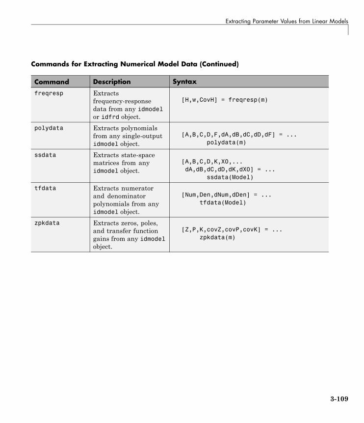
Extracting Parameter Values from Linear Models
Commands for Extracting Numerical Model Data (Continued)
Command Description Syntax
freqresp Extractsfrequency-responsedata from any idmodelor idfrd object.
[H,w,CovH] = freqresp(m)
polydata Extracts polynomialsfrom any single-outputidmodel object.
[A,B,C,D,F,dA,dB,dC,dD,dF] = ...polydata(m)
ssdata Extracts state-spacematrices from anyidmodel object.
[A,B,C,D,K,X0,...dA,dB,dC,dD,dK,dX0] = ...
ssdata(Model)
tfdata Extracts numeratorand denominatorpolynomials from anyidmodel object.
[Num,Den,dNum,dDen] = ...tfdata(Model)
zpkdata Extracts zeros, poles,and transfer functiongains from any idmodelobject.
[Z,P,K,covZ,covP,covK] = ...zpkdata(m)
3-109

3 Linear Model Identification
Extracting Dynamic Model and Noise Model SeparatelyYou can extract the numerical data associated with a dynamic model andthe noise model separately.
For linear models, the general symbolic model description is given by:
y Gu He= +
G is an operator that takes the measured inputs u to the outputs and capturesthe system dynamics. H is an operator that describes the properties of theadditive output disturbance and takes the hypothetical (unmeasured) noisesource inputs e to the outputs, also called the noise model. When you estimatea noise model, the toolbox includes one noise channel e at the input for eachoutput in your system.
The following table summarizes the results of ssdata, tfdata, and zpkdatacommands for extracting the numerical values of the dynamic model andnoise model separately. fcn represents ssdata, tfdata, and zpkdata, andm is a model object. L represents the covariance matrix e, as defined in“Subreferencing Measured and Noise Models” on page 3-120.
For information about subreferencing noise channels or treating noisechannels as measured input, see “Subreferencing Model Objects” on page3-119.
Note The syntax fcn(m('noise')) is equivalent to fcn(m('n')).
Syntax for Extracting Transfer-Function Data
Command Syntax
fcn(m) Returns the properties of G for ny outputs and nu inputs.fcn(m('noise')) Returns the properties of H for ny outputs and ny inputs.fcn(noisecnv(m)) Returns the properties of [G H] ny outputs and ny+nu
inputs.
3-110

Extracting Dynamic Model and Noise Model Separately
Syntax for Extracting Transfer-Function Data (Continued)
Command Syntax
fcn(noisecnv(m,'Norm')) Returns the properties of [G HL] ny outputs and ny+nuinputs.
fcn(noisecnv(m('noise'),'Norm')) Returns the properties of HL ny outputs and ny inputs.fcn(m) If m is a time-series model, returns the properties of H.fcn(noisecnv(m,'Norm')) If m is a time-series model, returns the properties of HL.
Note The estimated covariance matrix NoiseVariance is uncertain. Thus,the uncertainty of H differs from the uncertainty of HL.
3-111

3 Linear Model Identification
Transforming Between Discrete-Time and Continuous-TimeRepresentations
In this section...
“Why Transform Between Continuous and Discrete Time?” on page 3-112“Using the c2d, d2c, and d2d Commands” on page 3-112“Specifying Intersample Behavior” on page 3-114“How d2c Handles Input Delays” on page 3-114“Effects on the Noise Model” on page 3-115
Why Transform Between Continuous and DiscreteTime?Transforming between continuous-time and discrete-time representations isuseful, for example, if you have estimated a discrete-time linear model andrequire a continuous-time model instead.
d2d is useful is you want to change the sampling interval of a discretemodel. All of these operations change the sampling interval, which is calledresampling the model.
Using the c2d, d2c, and d2d CommandsYou can use c2d and d2c to transform any idmodel object betweencontinuous-time and discrete-time representations.
The following table summarizes the commands for transforming betweencontinuous-time and discrete-time model representations. These commandsalso transform the estimated model uncertainty, which corresponds to theestimated covariance matrix of the parameters. For detailed informationabout these commands, see the corresponding reference page.
3-112

Transforming Between Discrete-Time and Continuous-Time Representations
Note c2d and d2d correctly approximate the transformation of the noisemodel when the sampling interval T is small compared to the bandwidthof the noise.
Command Description Usage Example
c2d Convertscontinuous-timemodels to discrete-timemodels.
To transform a continuous-timemodel mod_c to a discrete-timeform, use the followingcommand:
mod_d = c2d(mod_c,T)
where T is the sampling intervalof the discrete-time model.
d2c Converts parametricdiscrete-time modelsto continuous-timemodels.
To transform a discrete-timemodel mod_d to acontinuous-time form, usethe following command:
mod_c = d2c(mod_d)
d2d Resample a lineardiscrete-timemodel and producean equivalentdiscrete-time modelwith a new samplinginterval.You can use theresampled model tosimulate or predictoutput with a specifiedtime interval.
To resample a discrete-timemodel mod_d1 to a discrete-timeform with a new samplinginterval Ts, use the followingcommand:
mod_d2 = d2d(mod_d1,Ts)
3-113

3 Linear Model Identification
The following commands compare estimated model m and its continuous-timecounterpart mc on a Bode plot:
% Estimate discrete-time ARMAX model% from the datam = armax(data,[2 3 1 2]);% Convert to continuous-time formmc = d2c(m);% Plot bode plot for both modelsbode(m,mc)
Specifying Intersample BehaviorA sampled signal is characterized only by its values at the sampling instants.However, when you apply a continuous-time input to a continuous-timesystem, the output values at the sampling instants depend on the inputs atthe sampling instants and on the inputs between these points. Thus, theInterSample data property describes how the algorithms should handle theinput between samples. For example, you can specify the behavior betweenthe samples to be piece-wise constant (zero-order hold, zoh) or linearlyinterpolated between the samples (first order hold, foh). The transformationformulas for c2d and d2c are affected by the intersample behavior of the input.
By default, c2d and d2c use the intersample behavior you assigned to theestimation data. To override this setting during transformation, add an extraargument in the syntax. For example:
% Set first-order hold intersample behaviormod_d = c2d(mod_c,T,'foh')
How d2c Handles Input DelaysThe discrete-to-continuous-time conversion d2c properly handles anyinput delays in the discrete-time model, and stores this information in thecontinuous-time model. An input delay is the delay in the response of theoutput to the input signal.
The relationship between discrete-time and continuous-time delays dependson the input intersample behavior. For example, a continuous-time systemwithout a delay shows a delay when sampled with a zero-order-hold input.
3-114

Transforming Between Discrete-Time and Continuous-Time Representations
A delay in the discrete-time model that corresponds to an actual delay in thecontinuous-time model is stored in the in the InputDelay property of theresulting continuous-time model. Typically, this InputDelay is (nk-1)/Ts,where nk is the delay of the discrete-time system and Ts is the samplinginterval.
Note Unlike for discrete-time models, the nk property of continuous-timemodel is only used to flag when immediate response to step changes is present;nk is not used to store input delays greater than or equal to 1. When nk(i)=0,then there is an immediate response to a step change in the input ith. Whennk(i)=1, then there is no immediate response to the input.
Effects on the Noise Modelc2d, d2c, and d2d change the sampling interval of both the dynamic model andthe noise model. Resampling a model affects the variance of its noise model.
A parametric noise model is a time-series model with the followingmathematical description:
y t H q e t
Ee
( ) ( ) ( )=
=2 λ
The noise spectrum is computed by the following discrete-time equation:
Φvi TT H e( )ω λ ω= ( ) 2
where λ is the variance of the white noise e(t), and λT represents the spectraldensity of e(t). Resampling the noise model preserves the spectral density λT. The spectral density λT is invariant up to the Nyquist frequency. For moreinformation about spectrum normalization, see “Understanding SpectrumNormalization” on page 3-11.
d2d resampling of the noise model affects simulations with noise usingsim. If you resample a model to a faster sampling rate, simulating thismodel results in higher noise level. This higher noise level results from the
3-115
3 Linear Model Identification
underlying continuous-time model being subject to continuous-time whitenoise disturbances, which have infinite, instantaneous variance. In thiscase, the underlying continuous-time model is the unique representation fordiscrete-time models. To maintain the same level of noise after interpolating
the noise signal, scale the noise spectrum by TT
New
Old, where Tnew is the new
sampling interval and Told is the original sampling interval. before applyingsim.
c2d and d2c transformations produce warnings when the continuous-timedisturbance model does not have the required white-noise component.These warnings occur because the underlying state-space model, whichis formed and used by these transformations, is ill-defined. In this case,modify the C-polynomial such that the degree of the monic C-polynomialin continuous-time equals the sum of the degrees of the monic A- andD-polynomials in continuous-time. For example:
length(C)-1 = (length(A)-1)+(length(D)-1)
3-116

Transforming Between Linear Model Representations
Transforming Between Linear Model RepresentationsYou can transform linear models between state-space and polynomial forms.You can also transform between frequency-response, state-space, andpolynomial forms.
If you used the System Identification Tool GUI to estimate models, you mustexport the models to the MATLAB workspace before converting models.
For detailed information about each command in the following table, see thecorresponding reference page.
Commands for Transforming Model Representations
Command Model Type to Convert Usage Example
idfrd Converts any single- ormultiple-output idmodelobject to idfrd model.If you have the ControlSystem Toolbox product, thiscommand converts any LTIobject.
To get frequency response of m at defaultfrequencies, use the following command:
m_f = idfrd(m)
To get frequency response at specificfrequencies, use the following command:
m_f = idfrd(m,f)
To get frequency response for a submodelfrom input 2 to output 3, use thefollowing command:
m_f = idfrd(m(2,3))
3-117

3 Linear Model Identification
Commands for Transforming Model Representations (Continued)
Command Model Type to Convert Usage Example
idpoly Converts single-outputidmodel object to ARMAXrepresentation.If you have the ControlSystem Toolbox product,this command converts anysingle-output LTI objectexcept frd.
To get an ARMAXmodel from state-spacemodel m_ss, use the following command:
m_p = idpoly(m_ss)
idss Converts any single- ormultiple-output idmodelobject to state-spacerepresentation.If you have the ControlSystem Toolbox product, thiscommand converts any LTIobject except frd.
To get a state-space model from an ARXmodel m_arx, use the following command:
m_ss = idss(m_arx)
Note The idss conversion produces warnings when the continuous-timedisturbance model does not have the required white-noise component.These warnings occur because the underlying state-space model, whichis formed and used by these transformations, is ill defined. In this case,modify the C-polynomial such that the degree of the monic C-polynomialin continuous-time equals the sum of the degrees of the monic A- andD-polynomials in continuous-time. For example:
length(C)-1 = (length(A)-1)+(length(D)-1)
3-118
Subreferencing Model Objects
Subreferencing Model Objects
In this section...
“What Is Subreferencing?” on page 3-119“Limitation on Supported Models” on page 3-119“Subreferencing Specific Measured Channels” on page 3-119“Subreferencing Measured and Noise Models” on page 3-120“Treating Noise Channels as Measured Inputs” on page 3-122
What Is Subreferencing?You can use subreferencing to create models with subsets of inputs andoutputs from existing multivariable models. Subreferencing is also usefulwhen you want to generate model plots for only certain channels, such aswhen you are exploring multiple-output models for input channels that haveminimal effect on the output.
The toolbox supports subreferencing operations for idarx, idgrey, idpoly,idproc, idss, and idfrd model objects.
In addition to subreferencing the model for specific combinations of measuredinputs and output, you can subreference dynamic and noise modelsindividually.
Limitation on Supported ModelsSubreferencing nonlinear models is not supported.
Subreferencing Specific Measured ChannelsUse the following general syntax to subreference specific input and outputchannels in models:
model(outputs,inputs)
In this syntax, outputs and inputs specify channel indexes or channel names.
3-119
3 Linear Model Identification
To select all output or all input channels, use a colon (:). To select nochannels, specify an empty matrix ([]). If you need to reference severalchannel names, use a cell array of strings.
For example, to create a new model m2 from m from inputs 1 ('power') and4 ('speed') to output number 3 ('position'), use either of the followingequivalent commands:
m2 = m('position',{'power','speed'})
or
m2 = m(3,[1 4])
For a single-output model, you can use the following syntax to subreferencespecific input channels without ambiguity:
m3 = m(inputs)
Similarly, for a single-input model, you can use the following syntax tosubreference specific output channels:
m4 = m(outputs)
Subreferencing Measured and Noise ModelsFor linear models, the general symbolic model description is given by:
y Gu He= +
G is an operator that takes the measured inputs u to the outputs and capturesthe system dynamics.
H is an operator that describes the properties of the additive outputdisturbance and takes the hypothetical (unmeasured) noise source inputs tothe outputs. H represents the noise model. When you specify to estimate anoise model, the resulting model include one noise channel e at the input foreach output in your system.
3-120

Subreferencing Model Objects
Thus, linear, parametric models represent input-output relationships for twokinds of input channels: measured inputs and (unmeasured) noise inputs. Forexample, consider the ARX model given by one of the following equations:
A q y t B q u t nk e t( ) ( ) ( ) ( )= −( ) +
or
y tB qA q
u tA q
e t( )( )( ) ( )
( )= ( ) + 1
In this case, the dynamic model is the relationship between the measured
input u and output y, G B qA q= ( )
( ) . The noise model is the contribution of the
input noise e to the output y, given byH A q= 1( ) .
Suppose that the model m contains both a dynamic model G and a noise modelH. To create a new model by subreferencing G due to measured inputs, usethe following syntax:
m_G = m('measured')
Tip Alternatively, you can use the following shorthand syntax: m_G = m('m')
3-121

3 Linear Model Identification
To create a new model by subreferencing H due to unmeasured inputs, usethe following syntax:
m_H = m('noise')
Tip Alternatively, you can use the following shorthand syntax: m_H = m('n')
This operation creates a time-series model from m by ignoring the measuredinput.
The covariance matrix of e is given by the idmodel property NoiseVariance,which is the matrix Λ :
Λ = LLT
The covariance matrix of e is related to v, as follows:
e Lv=where v is white noise with an identity covariance matrix representingindependent noise sources with unit variances.
Treating Noise Channels as Measured InputsTo study noise contributions in more detail, it might be useful to convert thenoise channels to measured channels using noisecnv:
m_GH = noisecnv(m)
This operation creates a model m_GH that represents both measured inputs uand noise inputs e, treating both sources as measured signals. m_GH is a modelfrom u and e to y, describing the transfer functions G and H.
3-122

Subreferencing Model Objects
Converting noise channels to measured inputs loses information aboutthe variance of the innovations e. For example, step response due to thenoise channels does not take into consideration the magnitude of the noisecontributions. To include this variance information, normalize e such that vbecomes white noise with an identity covariance matrix, where
e Lv=
To normalize e, use the following command:
m_GH = noisecnv(m,'Norm')
This command creates a model where u and v are treated as measuredsignals, as follows:
y t Gu t HLv G HLuv
( ) ( )= + = [ ]⎡⎣⎢⎤
⎦⎥
For example, the scaling by L causes the step responses from v to y to reflectthe size of the disturbance influence.
The converted noise sources are named in a way that relates the noise channelto the corresponding output. Unnormalized noise sources e are assignednames such as 'e@y1', 'e@y2', ..., 'e@yn', where 'e@yn' refers to the noiseinput associated with the output yn. Similarly, normalized noise sources v,are named 'v@y1', 'v@y2', ..., 'v@yn'.
Note When you plot models in the GUI that include noise sources, youcan select to view the response of the noise model corresponding to specificoutputs. For more information, see “Selecting Measured and Noise Channelsin Plots” on page 12-18.
3-123
3 Linear Model Identification
Concatenating Model Objects
In this section...
“About Concatenating Models” on page 3-124“Limitation on Supported Models” on page 3-124“Horizontal Concatenation of Model Objects” on page 3-125“Vertical Concatenation of Model Objects” on page 3-125“Concatenating Noise Spectral Data of idfrd Objects” on page 3-126“See Also” on page 3-127
About Concatenating ModelsYou can perform horizontal and vertical concatenation of linear model objectsto grow the number of inputs or outputs in the model.
When you concatenate parametric models, such as idarx, idgrey, idpoly,idproc, and idss model objects, the resulting model combines the parametersof the individual models.
You can also concatenate nonparametric models, which contain the estimatedimpulse-response (idarx object) and frequency-response (idfrd object) of asystem.
In case of idfrd models, concatenation combines information in theResponseData properties of the individual model objects. ResponseData isan ny-by-nu-by-nf array that stores the response of the system, where nyis the number of output channels, nu is the number of input channels, andnf is the number of frequency values. The (j,i,:) vector of the resultingresponse data represents the frequency response from the ith input to thejth output at all frequencies.
Limitation on Supported ModelsConcatenation is supported for linear models only.
3-124
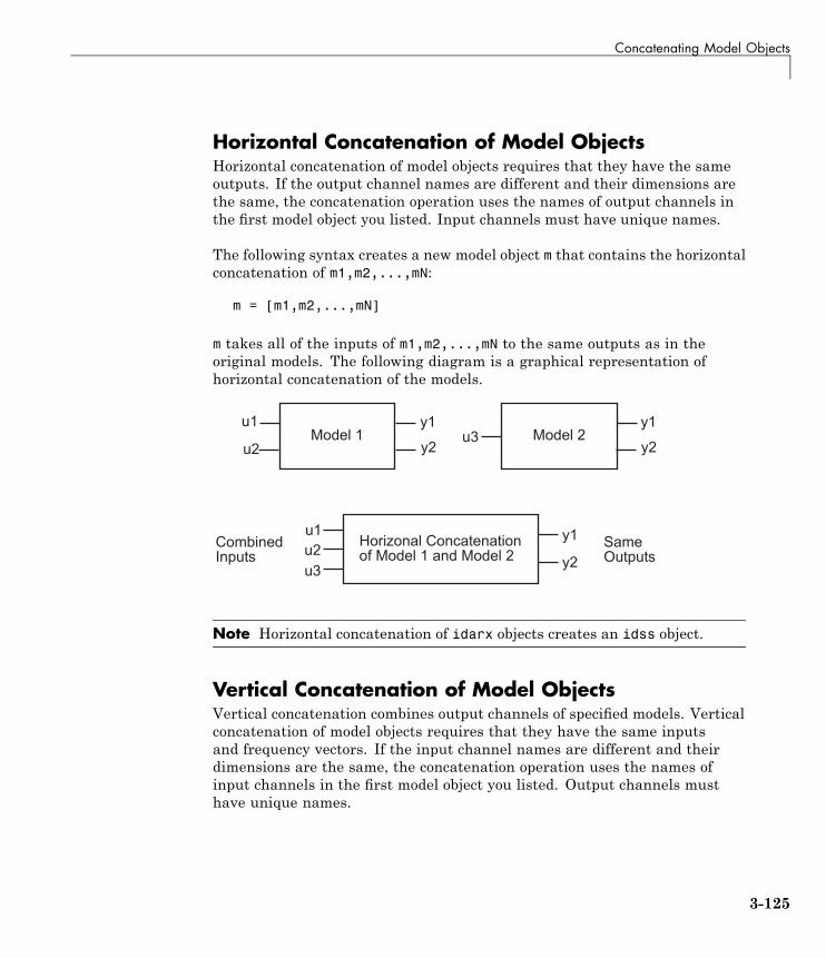
Concatenating Model Objects
Horizontal Concatenation of Model ObjectsHorizontal concatenation of model objects requires that they have the sameoutputs. If the output channel names are different and their dimensions arethe same, the concatenation operation uses the names of output channels inthe first model object you listed. Input channels must have unique names.
The following syntax creates a new model object m that contains the horizontalconcatenation of m1,m2,...,mN:
m = [m1,m2,...,mN]
m takes all of the inputs of m1,m2,...,mN to the same outputs as in theoriginal models. The following diagram is a graphical representation ofhorizontal concatenation of the models.
(����� (�����
�� ������� �������������(����������(�����
��
���!
�����!
��
��
��
��
��
�� "��)������
������*�����
Note Horizontal concatenation of idarx objects creates an idss object.
Vertical Concatenation of Model ObjectsVertical concatenation combines output channels of specified models. Verticalconcatenation of model objects requires that they have the same inputsand frequency vectors. If the input channel names are different and theirdimensions are the same, the concatenation operation uses the names ofinput channels in the first model object you listed. Output channels musthave unique names.
3-125

3 Linear Model Identification
Note You cannot concatenate the single-output idproc and idpoly modelobjects.
The following syntax creates a new model object m that contains the verticalconcatenation of m1,m2,...,mN:
m = [m1;m2;... ;mN]
m takes the same inputs in the original models to all of the output ofm1,m2,...,mN. The following diagram is a graphical representation of verticalconcatenation of frequency-response data.
(����� (�����
# ����� �������������(����������(�����
��
���!
��
��
��
��
����
������)������
"��*�����
�!
��
��
Concatenating Noise Spectral Data of idfrd ObjectsWhen the idfrd objects contain the frequency-response data you measuredor constructed manually, the concatenation operation combines only theResponseData properties. Because noise spectral data does not exist (unlessyou also entered it manually), SpectralData is empty in both the individualidfrd objects and the concatenated idfrd object.
However, when the idfrd objects are spectral models that you estimated, theSpectralData property is not empty and contains the power spectra andcross spectra of the output noise in the system. For each output channel, thistoolbox estimates one noise channel to explain the difference between theoutput of the model and the measured output.
3-126

Concatenating Model Objects
When the SpectralData property of individual idfrd objects is not empty,horizontal and vertical concatenation handle SpectralData, as follows.
In case of horizontal concatenation, there is no meaningful way to combine theSpectralData of individual idfrd objects, and the resulting SpectralDataproperty is empty. An empty property results because each idfrd object hasits own set of noise channels, where the number of noise channels equals thenumber of outputs. When the resulting idfrd object contains the same outputchannels as each of the individual idfrd objects, it cannot accommodate thenoise data from all the idfrd objects.
In case of vertical concatenation, this toolbox concatenates individual noisemodels diagonally. The following shows that m.SpectrumData is a blockdiagonal matrix of the power spectra and cross spectra of the output noise inthe system:
m sm s
mN s
..
.
=
⎛
⎝
⎜⎜⎜⎜
⎞
⎠
⎟⎟⎟⎟
1 0
0�
s in m.s is the abbreviation for the SpectrumData property name.
See AlsoIf you have the Control System Toolbox product, see “Combining ModelObjects” on page 10-6 about additional functionality for combining models.
3-127
3 Linear Model Identification
Merging Model ObjectsYou can merge models of the same structure to obtain a single model withparameters that are statistically weighed means of the parameters of theindividual models. When computing the merged model, the covariancematrices of the individual models determine the weights of the parameters.
You can perform the merge operation for the idarx, idgrey, idpoly, idproc,and idss model objects.
Note Each merge operation merges the same type of model object.
Merging models is an alternative to merging data sets into a singlemultiexperiment data set, and then estimating a model for the merged data.Whereas merging data sets assumes that the signal-to-noise ratios are aboutthe same in the two experiments, merging models allows greater variationsin model uncertainty, which might result from greater disturbances in anexperiment.
When the experimental conditions are about the same, merge the datainstead of models. This approach is more efficient and typically involvesbetter-conditioned calculations. For more information about merging datasets into a multiexperiment data set, see “Creating Multiexperiment Data atthe Command Line” on page 1-53.
For more information about merging models, see the merge reference page.
3-128

4
Nonlinear Black-Box ModelIdentification
• “Supported Data for Estimating Nonlinear Black-Box Models” on page 4-2
• “Supported Nonlinear Black-Box Models” on page 4-3
• “Identifying Nonlinear ARX Models” on page 4-4
• “Identifying Hammerstein-Wiener Models” on page 4-15
• “Supported Nonlinearity Estimators” on page 4-25
• “Refining Nonlinear Black-Box Models” on page 4-28
• “Extracting Parameter Values from Nonlinear Black-Box Models” on page4-30
• “Next Steps After Estimating Nonlinear Black-Box Models” on page 4-32
• “Computing Linear Approximations of Nonlinear Black-Box Models” onpage 4-33

4 Nonlinear Black-Box Model Identification
Supported Data for Estimating Nonlinear Black-BoxModels
You can estimate discrete-time black-box models for data with the followingcharacteristics:
• Time-domain input-output or time-series data.
Note Time series are supported for nonlinear ARX models only.
• Single-output or multiple-output data.
Before you begin estimating models, import your data into the MATLABsoftware and represent the data in either of the following ways:
• In the System Identification Tool GUI. Import the data into the GUI,as described in “Representing Data in the GUI” on page 1-13.
• At the command line. Represent your data as an iddata or idfrd object.
To examine the data features, plot the data on a time plot or an estimatedfrequency-response plot. You can preprocess your data by interpolatingmissing values, filtering to emphasize a specific frequency range, orresampling using a different time interval. For more information aboutavailable date plots and data-preprocessing operations, see Chapter 1, “DataProcessing”.
Caution For nonlinear modeling, do not remove offsets and linear trendsfrom the measured signals.
4-2

Supported Nonlinear Black-Box Models
Supported Nonlinear Black-Box ModelsYou can estimate the following types of nonlinear black-box models:
• Nonlinear ARX models
• Hammerstein-Wiener models
You can estimate these models both in the System Identification Tool GUIand at the command line.
For an introduction, see “Tutorial – Identifying Nonlinear Black-Box ModelsUsing the GUI” in the System Identification Toolbox Getting Started Guide.
4-3
4 Nonlinear Black-Box Model Identification
Identifying Nonlinear ARX Models
In this section...
“Supported Data for Nonlinear ARX Models” on page 4-4“Definition of the Nonlinear ARX Model” on page 4-4“Using Regressors” on page 4-6“Nonlinearity Estimators for Nonlinear ARX Models” on page 4-9“How to Estimate Nonlinear ARX Models in the GUI” on page 4-10“How to Estimate Nonlinear ARX Models at the Command Line” on page4-11
Supported Data for Nonlinear ARX ModelsYou can estimate discrete-time nonlinear ARX models from data with thefollowing characteristics:
• Time-domain input-output data or time-series data
• Single-output or multiple-output data
For more information about representing your data for system identification,see Chapter 1, “Data Processing”.
Definition of the Nonlinear ARX ModelNonlinear ARX models describe nonlinear structures using a parallelcombination of nonlinear and linear blocks. The nonlinear and linearfunctions are expressed in terms of variables called regressors.
The System Identification Toolbox product computes regressors by performingtransformations of the measured input u(t) and output y(t) signals basedon the model order you specify. For example, regressors can be delayedinputs and outputs, such as u(t-1) and y(t-3). Regressors can also be nonlinearfunctions of inputs and outputs, such as tan(u(t-1)) or u(t-1)y(t-3). You caneither use default regressors, or specify your own custom functions of inputand output signals.
4-4

Identifying Nonlinear ARX Models
The predicted output ˆ( )y t of a nonlinear model at time t is given by thefollowing general equation:
ˆ( ) ( ( ))y t F x t=
where x(t) represents the regressors. F is a nonlinear regression function,which is approximated by a nonlinearity estimator, which might be a binarypartition tree, a neural network, or a network based on wavelets. Thefollowing figure shows how the predicted output of the model is formed fromthe inputs and outputs.
����������+������ �������
, ����)������
*������-�.
)�������-�.
��-���./��-��!./��-���./�&&& 0��� �������
The function F can include both linear and nonlinear functions of x(t), asshown in the previous diagram. You can specify which regressors to use ainputs to the nonlinear block.
The following equation provides a general description of F:
F x xkk
d
k k( ) = −( )( )=∑α κ β γ
1
where κ is the unit nonlinear function, d is the number of nonlinearity units,and αk , βk , and γk are the parameters of the nonlinearity estimator.
You choose a nonlinear structure that independently combines linear andnonlinear regressors and the structure of the nonlinearity itself, such astreepartition or wavenet. The System Identification Toolbox product usesinput/output data to find the linear and nonlinear mappings that give the bestpredicted outputs of the nonlinear model.
4-5

4 Nonlinear Black-Box Model Identification
For more information about regressors, see “Using Regressors” on page 4-6.For a list of nonlinearity estimators supported by nonlinear ARX models, see“Nonlinearity Estimators for Nonlinear ARX Models” on page 4-9.
Using RegressorsYou can use the following types of regressors for nonlinear ARX models:
• Standard regressors — Past input u(t) and output signals y(t), computedautomatically as delay transformations for specified model orders.
• Custom regressors — Products, powers, and other MATLAB expressionsof input and output variables that you specify.
Specifying Model Order and DelaysYou must specify the following model orders for computing standardregressors:
• na— The number of past output terms used to predict the current output.
• nb— The number of past input terms used to predict the current output.
• nk— The delay from input to the output in terms of the number of samples.This value defines the least delayed input regressor.
The meaning of na and nb is similar to the linear-ARX model parameters inthe sense that na represents the number of output terms and nb represents thenumber of input terms. nk represents the minimum input delay from an inputto an output. For more information about the linear ARX model structure, see“What Are Black-Box Polynomial Models?” on page 3-41.
Note The total number of regressors in the model must be greater than zero.If you only need to use custom regressors, set na=nb=nk=0 to omit creatingstandard regressors.
4-6
Identifying Nonlinear ARX Models
Example – Relationship Between Regressors, Model Orders,and DelaysThis example describes how the model orders and delays you specify relateto computing the regressors.
Suppose that you specify a nonlinear ARX model with a minimum of atwo-sample input delay and the number of input terms is nb=2. The toolboxcomputes the following standard regressors from the input signal:
• u(t-2)
• u(t-3)
If you specify that the number of output terms is na=4, the toolbox computesthe following standard regressors from the output signals:
• y(t-1)
• y(t-2)
• y(t-3)
• y(t-4)
Note The minimum output delay is fixed at 1 because the prediction ofan output requires the delayed versions of itself and all other outputs.To use past outputs for predicting the current value, you must includepast output samples, starting with the most recent at t=-1. In the caseof decoupled outputs, the delay for output signals corresponding to theprediction horizon. To use greater output delay values (for example, 2), youmust explicitly exclude the regressors that correspond to a delay of 1 (suchas y_i(t-1)) for the nonlinear block during estimation by configuring theNonlinearRegressors model property. However, all regressors are used inthe linear block if the linear block is included in your model.
If you have physical insight that your current output depends on specificdelayed inputs and outputs, select the appropriate model orders to computethe required regressors.
4-7

4 Nonlinear Black-Box Model Identification
Using Custom RegressorsIn general, custom regressors are nonlinear functions of delayed input andoutput data samples. You can specify custom regressors, such as tan(u(t-1)),u(t-1)2, or u(t-1)*y(t-3).
In the System Identification Tool GUI. You can create custom regressorsin the Model Regressors dialog box. For more information, see “How toEstimate Nonlinear ARX Models in the GUI” on page 4-10.
At the command line. Use the customreg or polyreg command to constructcustom regressors in terms of input-output variables. For more information,see the corresponding reference page.
The linear block includes all standard and custom regressors. However, youcan include specific standard and custom regressors in your nonlinear block tofine-tune the model structure.
To get a linear-in-the-parameters ARX model structure, you can excludethe nonlinear block from the model structure completely. When usingonly a linear block with custom regressors, you can create the simplesttypes of nonlinear models. In this case, the custom regressors capturethe nonlinearities and the estimation routine computes the weights of thestandard and custom regressors in the linear block to predict the output.
4-8
Identifying Nonlinear ARX Models
Nonlinearity Estimators for Nonlinear ARX ModelsNonlinear ARX models support the following nonlinearity estimators:
• Sigmoid Network
• Tree Partition
• Wavelet Network
• Custom Network
• Linear (indicates absence of nonlinearity estimator)
• Neural Network
Note You must have the Neural Network Toolbox™ product to usethe Neural Network nonlinearity estimator. If your model has only oneregressor, you can also use the Saturation, Dead Zone, One-DimensionalPolynomial, and Piecewise Linear nonlinearity estimators, as listed in“Nonlinearity Estimators for Hammerstein-Wiener Models” on page 4-17.
For a summary of all nonlinearity estimators and links to the correspondingreference pages, see “Supported Nonlinearity Estimators” on page 4-25.
You can exclude the nonlinearity function from the model structure. In thiscase, the model includes all standard and custom regressors and is linear inthe parameters.
In the System Identification Tool GUI. You can omit the nonlinear blockby selecting None for the Nonlinearity.
At the command line. You can omit the nonlinear block by setting theNonlinearity property value to 'Linear'. For more information, see thenlarx and idnlarx reference pages.
For a description of each nonlinearity estimator, see “Supported NonlinearityEstimators” on page 4-25.
4-9

4 Nonlinear Black-Box Model Identification
How to Estimate Nonlinear ARX Models in the GUI
You must have already imported your data into the System IdentificationTool GUI. For more information about preparing your data, see Chapter 1,“Data Processing”.
To estimate a nonlinear ARX model in the System Identification Tool GUI:
1 In the System Identification Tool GUI, select Estimate > Nonlinearmodels to open the Nonlinear Models dialog box. The Model Type tabis selected.
2 In the Model Structure list, select Nonlinear ARX.
This action updates the options in the Nonlinear Models dialog box tocorrespond to this model structure. For information about this modelstructure, see “Definition of the Nonlinear ARX Model” on page 4-4.
3 In the Model name field, edit the name of the model, or keep the defaultname. The name of the model should be unique to all nonlinear ARXmodels in the System Identification Tool GUI.
4 (Optional) If you want to try refining a previously estimated model, selectthe name of this model in the Initial model list.
Note The model structure and algorithm properties of the initial modelpopulate the fields in the Nonlinear Models dialog box.
A model is available in the Initial model list under the followingconditions:
• The model exists in the System Identification Tool GUI.
• The number of model inputs and outputs matches the dimensionsof the Working Data (estimation data) you selected in the SystemIdentification Tool GUI.
5 Keep the default settings in the Nonlinear Models dialog box that specifythe model structure and the algorithm, or modify the following settings:
4-10

Identifying Nonlinear ARX Models
• In the Regressors tab, change the input delay of the input signals.
To gain insight into possible input delay values, click Infer InputDelay. This action opens the Infer Input Delay dialog box.
• In the Regressors tab, change the number of terms to include in thenonlinear block.
• In the Regressors tab, click Edit Regressors to select which regressorsare included in the nonlinear block. This action opens the ModelRegressors dialog box. You can also use this dialog box to create customregressors.
• In the Model Properties tab, select and configure the nonlinearityestimator, and choose whether to include the linear block. To use allstandard and custom regressors in the linear block only, you can excludethe nonlinear block by choosing None.
For more information about the available options, click Help in theNonlinear Models dialog box to open the GUI help.
6 Click Estimate to add this model to the Model Board in the SystemIdentification Tool GUI.
The Estimation tab displays the estimation progress and results.
7 To plot the response of this model, select the appropriate check box inthe Model Views area of the System Identification Tool GUI. If you getan inaccurate fit, try estimating a new model with different orders ornonlinearity estimator. For more information about validating models, seeChapter 8, “Model Analysis”.
8 For further analysis, export the model to the MATLAB workspace bydragging it to the To Workspace rectangle in the System IdentificationTool GUI.
How to Estimate Nonlinear ARX Models at theCommand Line
• “General nlarx Syntax” on page 4-12
• “Example – Using nlarx to Estimate Nonlinear ARX Models” on page 4-13
4-11

4 Nonlinear Black-Box Model Identification
General nlarx SyntaxYou can estimate nonlinear ARX models using nlarx. The resulting modelsare stored as idnlarx model objects.
Use the following general syntax to both configure and estimate nonlinearARX models:
m = nlarx(data,'na',na,...'nb',nb,...'nk',nk,...Nonlinearity,...
'Property1',Value1,...,'PropertyN',ValueN)
where data is the estimation data. na, nb, and nk specify the model ordersand delays. For more information about model orders, see “Specifying ModelOrder and Delays” on page 4-6.
Nonlinearity specifies the nonlinearity estimator object as 'sigmoidnet','wavenet', 'treepartition', 'customnet', 'neuralnet', or 'linear'.
The property-value pairs specify any idnlarx model properties that configurethe estimation algorithm. You can enter all model property-value pairs andtop-level algorithm properties as a comma-separated list in nlarx.
For multiple inputs and outputs, na, nb, and nk are described in “Options forMultiple-Input and Multiple-Output ARX Orders” on page 3-64.
You can specify different nonlinearity estimators for different output channelsby setting Nonlinearity to an object array. For example:
m = nlarx(data,[[2 1; 0 1] [2;1] [1;1]],...[wavenet;sigmoidnet('num',7)])
To specify the same nonlinearity for all outputs, set Nonlinearity to a singlenonlinearity estimator. For example:
m = nlarx(data,[[2 1; 0 1] [2;1] [1;1]],...sigmoidnet('num',7))
4-12
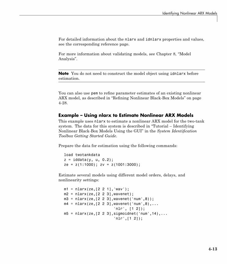
Identifying Nonlinear ARX Models
For detailed information about the nlarx and idnlarx properties and values,see the corresponding reference page.
For more information about validating models, see Chapter 8, “ModelAnalysis”.
Note You do not need to construct the model object using idnlarx beforeestimation.
You can also use pem to refine parameter estimates of an existing nonlinearARX model, as described in “Refining Nonlinear Black-Box Models” on page4-28.
Example – Using nlarx to Estimate Nonlinear ARX ModelsThis example uses nlarx to estimate a nonlinear ARX model for the two-tanksystem. The data for this system is described in “Tutorial – IdentifyingNonlinear Black-Box Models Using the GUI” in the System IdentificationToolbox Getting Started Guide.
Prepare the data for estimation using the following commands:
load twotankdataz = iddata(y, u, 0.2);ze = z(1:1000); zv = z(1001:3000);
Estimate several models using different model orders, delays, andnonlinearity settings:
m1 = nlarx(ze,[2 2 1],'wav');m2 = nlarx(ze,[2 2 3],wavenet);m3 = nlarx(ze,[2 2 3],wavenet('num',8));m4 = nlarx(ze,[2 2 3],wavenet('num',8),...
'nlr', [1 2]);m5 = nlarx(ze,[2 2 3],sigmoidnet('num',14),...
'nlr',[1 2]);
4-13

4 Nonlinear Black-Box Model Identification
Compare the resulting models by plotting the model outputs on top of themeasured output:
compare(zv, m1,m2,m3,m4,m5)
MATLAB software responds with the following plot.
4-14
Identifying Hammerstein-Wiener Models
Identifying Hammerstein-Wiener Models
In this section...
“Supported Data for Estimating Hammerstein-Wiener Models” on page 4-15“Definition of the Hammerstein-Wiener Model” on page 4-15“Nonlinearity Estimators for Hammerstein-Wiener Models” on page 4-17“How to Estimate Hammerstein-Wiener Models in the GUI” on page 4-18“How to Estimate Hammerstein-Wiener Models at the Command Line”on page 4-20
Supported Data for Estimating Hammerstein-WienerModelsYou can estimate discrete-time Hammerstein-Wiener models from data withthe following characteristics:
• Time-domain input-output data
Note Hammerstein-Wiener models do not support time-series data, whichhas no input signal.
• Single-output or multiple-output data
Definition of the Hammerstein-Wiener ModelHammerstein-Wiener models describe dynamic systems using one or twostatic nonlinear blocks in series with a linear block. Only the linear blockcontains dynamic elements.
The linear block is a discrete-time transfer function and the nonlinearblocks are implemented using nonlinearity estimators, such as saturation,wavenet, and deadzone.
4-15
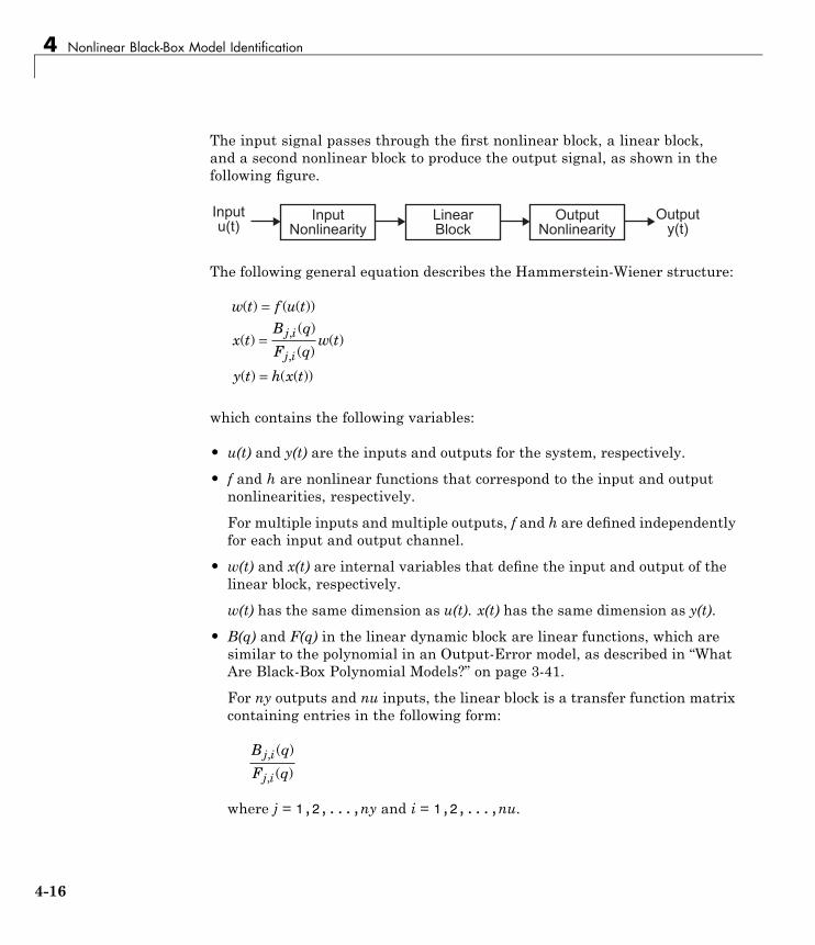
4 Nonlinear Black-Box Model Identification
The input signal passes through the first nonlinear block, a linear block,and a second nonlinear block to produce the output signal, as shown in thefollowing figure.
*�����-�.
)������-�.
*����+������ ���
0��� 1��$
)�����+������ ���
The following general equation describes the Hammerstein-Wiener structure:
w t f u t
x tB q
F qw t
y t h x t
j i
j i
( ) ( ( ))
( )( )
( )( )
( ) ( ( ))
,
,
=
=
=
which contains the following variables:
• u(t) and y(t) are the inputs and outputs for the system, respectively.
• f and h are nonlinear functions that correspond to the input and outputnonlinearities, respectively.
For multiple inputs and multiple outputs, f and h are defined independentlyfor each input and output channel.
• w(t) and x(t) are internal variables that define the input and output of thelinear block, respectively.
w(t) has the same dimension as u(t). x(t) has the same dimension as y(t).
• B(q) and F(q) in the linear dynamic block are linear functions, which aresimilar to the polynomial in an Output-Error model, as described in “WhatAre Black-Box Polynomial Models?” on page 3-41.
For ny outputs and nu inputs, the linear block is a transfer function matrixcontaining entries in the following form:
B q
F qj i
j i
,
,
( )
( )
where j = 1,2,...,ny and i = 1,2,...,nu.
4-16
Identifying Hammerstein-Wiener Models
If only the input nonlinearity is present, the model is called a Hammersteinmodel. If only the output nonlinearity is present, the model is called a Wienermodel.
You must specify the following model orders for the linear block:
• nb—The number of zeros plus one.
• nf—The number of poles.
• nk—The delay from input to the output in terms of the number of samples.
For ny outputs and nu inputs, nb, nf, and nk are ny-by-nu matrices. You canspecify a nonlinearity for only certain inputs and outputs, and exclude thenonlinearity for other inputs and outputs.
Nonlinearity Estimators for Hammerstein-WienerModelsHammerstein-Wiener models support the following nonlinearity estimatorsfor estimating the parameters of its input and output nonlinear blocks:
• Dead Zone
• Piecewise Linear
• Saturation
• Sigmoid Network
• Wavelet Network
• One-Dimensional Polynomial
• Unit Gain
• Custom Network
For a summary of all nonlinearity estimators and links to the correspondingreference pages, see “Supported Nonlinearity Estimators” on page 4-25.
You can exclude either the input nonlinearity or the output nonlinearity fromthe model structure:
4-17

4 Nonlinear Black-Box Model Identification
In the System Identification Tool GUI. Exclude a nonlinearity for aspecific channel by selecting None.
At the command line. Exclude a nonlinearity for a specific channelby specifying the unitgain value for the InputNonlinearity orOutputNonlinearity properties. For more information about estimationobjects and their properties, see nlhw and idnlhw reference page.
For a description of each nonlinearity estimator, see “Supported NonlinearityEstimators” on page 4-25.
How to Estimate Hammerstein-Wiener Models in theGUIYou must have already imported your data into the System Identification ToolGUI, as described in Chapter 1, “Data Processing”.
To estimate a Hammerstein-Wiener model in the System Identification ToolGUI:
1 In the System Identification Tool GUI, select Estimate > Nonlinearmodels to open the Nonlinear Models dialog box. TheModel Type tab isshown.
2 In the Model Structure list, select Hammerstein-Wiener.
This action updates the options in the Nonlinear Models dialog box tocorrespond to this model structure. For information about this modelstructure, see “Definition of the Hammerstein-Wiener Model” on page 4-15.
3 In the Model name field, edit the name of the model, or keep the defaultname. The name of the model should be unique to all Hammerstein-Wienermodels in the System Identification Tool GUI.
4-18

Identifying Hammerstein-Wiener Models
4 (Optional) If you want to try refining a previously estimated model, selectthe name of this model in the Initial model list.
Note The model structure and algorithm properties of the initial modelpopulate the fields in the Nonlinear Models dialog box.
A model is available in the Initial model list under the followingconditions:
• The model exists in the System Identification Tool GUI.
• The number of model inputs and outputs matches the dimensionsof the Working Data (estimation data) you selected in the SystemIdentification Tool GUI.
5 Keep the default settings in the Nonlinear Models dialog box that specifythe model structure and the algorithm, or modify the following settings:
• In the I/O Nonlinearity tab, specify whether to include or exclude theinput and output nonlinearities. For multiple-input and multiple-outputsystems, you can choose to apply nonlinearities only to specific inputand output channels.
• In the I/O Nonlinearity tab, change the input and output nonlinearitytypes and configure the nonlinearity settings.
Tip If you are not sure about which nonlinearity to try, start by usingthe Piecewise Linear nonlinearity estimator.
• In the Linear Block tab, specify the model orders and delays. To gaininsight into possible delays, click Infer Input Delay.
For more information about the available options, click Help in theNonlinear Models dialog box to open the GUI help.
6 Click Estimate to add this model to the Model Board in the SystemIdentification Tool GUI.
The Estimation tab displays the estimation progress and results.
4-19
4 Nonlinear Black-Box Model Identification
7 To plot the response of this model, select the appropriate check box inthe Model Views area of the System Identification Tool GUI. For moreinformation about working with plots and validating models, see Chapter8, “Model Analysis”.
If you get an inaccurate fit, try estimating a new model with different ordersor nonlinearity estimator.
You can export the model to the MATLAB workspace for further analysisby dragging it to the To Workspace rectangle in the System IdentificationTool GUI.
How to Estimate Hammerstein-Wiener Models at theCommand Line
• “General nlhw Syntax” on page 4-20
• “Improving Estimation Results Using Initial States” on page 4-22
• “Example – Using nlhw to Estimate Hammerstein-Wiener Models” on page4-23
General nlhw SyntaxYou can estimate Hammerstein-Wiener models using the nlhw command. Theresulting models are stored as idnlhw model objects.
Use the following general syntax to both configure and estimateHammerstein-Wiener models:
m = nlhw(data,'nb',nb,...'nf',nf,...'nk',nk,...InputNonlinearity,..OutputNonlinearity,...
'Property1',Value1,...,'PropertyN',ValueN)
where data is the estimation data. nb, nf, and nk specify the orders and delaysof the linear model, which is similar to an Output-Error (OE) model. For more
4-20

Identifying Hammerstein-Wiener Models
information about model orders, see “Definition of the Hammerstein-WienerModel” on page 4-15.
InputNonlinearity specifies the input static nonlinearity estimator objectas 'pwlinear', 'deadzone', 'saturation', 'sigmoidnet', 'wavenet','customnet', 'unitgain', or 'poly1d'. Similarly, OutputNonlinearityspecifies the output static nonlinearity estimator object.
The property-value pairs specify any idnlhw model properties that configurethe estimation algorithm. You can enter all model property-value pairsand top-level algorithm properties as a comma-separated list in nlhw. Forexample, you can control the iterative search for a best fit using the followingproperties:
m = nlhw(data,'nb',nb,...'nf',nf,...'nk',nk,...InputNonlinearity,...OutputNonlinearity,...
'MaxIter',N,...'Tolerance',tol,...'LimitError',lim,'Display','on')
Note You do not need to construct the model object using idnlhw beforeestimation. nlhw both constructs and estimates the model.
For nu inputs and ny outputs, na, nb, and nk are ny-by-nu matrices whosei-jth entry specifies the order and delay of the transfer function from thejth input to the ith output.
4-21

4 Nonlinear Black-Box Model Identification
You can specify different nonlinearity estimators for different output channelsby setting InputNonlinearity or OutputNonlinearity to an object array.For example, the following code estimates a two-input Hammerstein-Wienermodel, where sigmoidnet and pwlinear are the two input nonlinearitiesand there is no output nonlinearity:
m = nlhw(data,[nb,nf,nk],...[sigmoidnet;pwlinear],...[])
Alternatively, you can construct the model first and then estimate modelsparameters using the following commands:
m0 = idnlhw([nb,nf,nk],[sigmoidnet;pwlinear],[]);m = nlhw(data,m0);
For detailed information about nlhw and idnlhw, see the correspondingreference pages.
For more information about validating your models, see Chapter 8, “ModelAnalysis”.
You can also use pem to refine parameter estimates of an existingHammerstein-Wiener model, as described in “Refining Nonlinear Black-BoxModels” on page 4-28.
Improving Estimation Results Using Initial StatesIf your estimated Hammerstein-Wiener model provides a poor fit to measureddata, you can estimate the model again using initial states estimated fromthe data. By default, the initial states corresponding to the linear block of theHammerstein-Wiener model are zero.
To specify estimating initial states during model estimation, you can usethe following syntax:
m0 = idnlhw([nb,nf,nk],[sigmoidnet;pwlinear],[]);m = nlhw(data,m0,'InitialState','e');
4-22

Identifying Hammerstein-Wiener Models
Example – Using nlhw to Estimate Hammerstein-WienerModelsThis example uses nlhw to estimate a Hammerstein-Wiener model forthe two-tank system. The data for this system is described in “Tutorial –Identifying Nonlinear Black-Box Models Using the GUI” in the SystemIdentification Toolbox Getting Started Guide.
Prepare the data for estimation using the following commands:
load twotankdataz = iddata(y, u, 0.2);ze = z(1:1000); zv = z(1001:3000);
Estimate several models using different model orders, delays, andnonlinearity settings:
m1 = nlhw(ze,[2 3 1],'pwl','pwl');m2 = nlhw(ze,[2 2 3],'pwl','pwl');m3 = nlhw(ze,[2 2 3], pwlinear('num',13),...
pwlinear('num',10));m4 = nlhw(ze,[2 2 3], sigmoidnet('num',2),...
pwlinear('num',10));m5 = nlhw(ze,[2 2 3], 'dead','sat');
Compare the resulting models by plotting the model outputs on top of themeasured output:
compare(zv,m1,m2,m3,m4,m5)
4-23

4 Nonlinear Black-Box Model Identification
MATLAB software responds with the following plot.
4-24
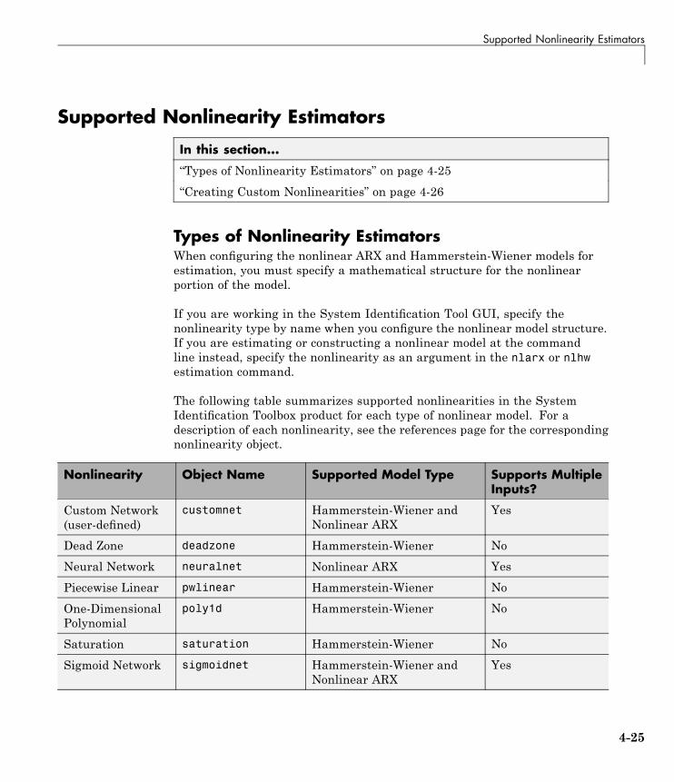
Supported Nonlinearity Estimators
Supported Nonlinearity Estimators
In this section...
“Types of Nonlinearity Estimators” on page 4-25“Creating Custom Nonlinearities” on page 4-26
Types of Nonlinearity EstimatorsWhen configuring the nonlinear ARX and Hammerstein-Wiener models forestimation, you must specify a mathematical structure for the nonlinearportion of the model.
If you are working in the System Identification Tool GUI, specify thenonlinearity type by name when you configure the nonlinear model structure.If you are estimating or constructing a nonlinear model at the commandline instead, specify the nonlinearity as an argument in the nlarx or nlhwestimation command.
The following table summarizes supported nonlinearities in the SystemIdentification Toolbox product for each type of nonlinear model. For adescription of each nonlinearity, see the references page for the correspondingnonlinearity object.
Nonlinearity Object Name Supported Model Type Supports MultipleInputs?
Custom Network(user-defined)
customnet Hammerstein-Wiener andNonlinear ARX
Yes
Dead Zone deadzone Hammerstein-Wiener NoNeural Network neuralnet Nonlinear ARX YesPiecewise Linear pwlinear Hammerstein-Wiener NoOne-DimensionalPolynomial
poly1d Hammerstein-Wiener No
Saturation saturation Hammerstein-Wiener NoSigmoid Network sigmoidnet Hammerstein-Wiener and
Nonlinear ARXYes
4-25
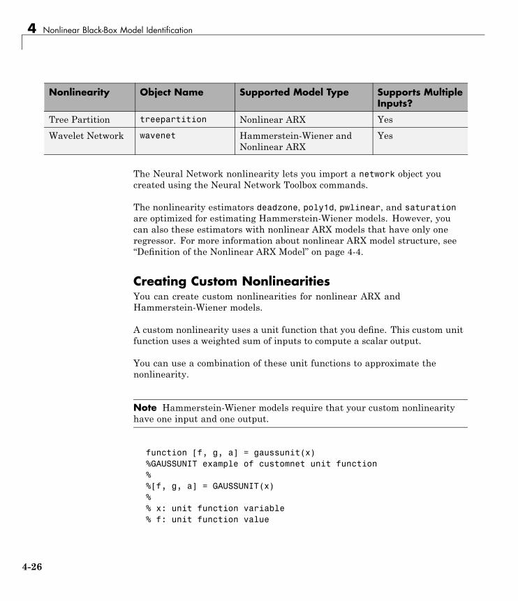
4 Nonlinear Black-Box Model Identification
Nonlinearity Object Name Supported Model Type Supports MultipleInputs?
Tree Partition treepartition Nonlinear ARX YesWavelet Network wavenet Hammerstein-Wiener and
Nonlinear ARXYes
The Neural Network nonlinearity lets you import a network object youcreated using the Neural Network Toolbox commands.
The nonlinearity estimators deadzone, poly1d, pwlinear, and saturationare optimized for estimating Hammerstein-Wiener models. However, youcan also these estimators with nonlinear ARX models that have only oneregressor. For more information about nonlinear ARX model structure, see“Definition of the Nonlinear ARX Model” on page 4-4.
Creating Custom NonlinearitiesYou can create custom nonlinearities for nonlinear ARX andHammerstein-Wiener models.
A custom nonlinearity uses a unit function that you define. This custom unitfunction uses a weighted sum of inputs to compute a scalar output.
You can use a combination of these unit functions to approximate thenonlinearity.
Note Hammerstein-Wiener models require that your custom nonlinearityhave one input and one output.
function [f, g, a] = gaussunit(x)%GAUSSUNIT example of customnet unit function%%[f, g, a] = GAUSSUNIT(x)%% x: unit function variable% f: unit function value
4-26

Supported Nonlinearity Estimators
% g: df/dx% a: unit active range (g(x) is significantly% nonzero in the interval [-a a])%% The unit function must be vectorized:% for a vector or matrix x, the output% arguments f and g must have the same size as x% f and g are computed element by element.
f = exp(-x.*x);
if nargout>1g = - 2*x .* f;a = 0.2;
end
4-27

4 Nonlinear Black-Box Model Identification
Refining Nonlinear Black-Box Models
In this section...
“How to Refine Nonlinear Black-Box Models in the GUI” on page 4-28“How to Refine Nonlinear Black-Box Models at the Command Line” onpage 4-29
How to Refine Nonlinear Black-Box Models in theGUIThe following procedure assumes that the model you want to refine is alreadyin the System Identification Tool GUI. You might have estimated this modelin the current session or imported the model into the GUI from the MATLABworkspace. For more information about estimating nonlinear black-boxmodels, see Chapter 4, “Nonlinear Black-Box Model Identification”.
To refine your model:
1 In the System Identification Tool GUI, verify that you have the correct dataset in the Working Data area for refining your model.
If you are using a different data set than the one you used to estimate themodel, drag the correct data set into the Working Data area. For moreinformation about specifying estimation data, see “Specifying Estimationand Validation Data” on page 1-29.
2 Select Estimate > Nonlinear models to open the Nonlinear Modelsdialog box, if this dialog box is not already open.
3 In the Nonlinear Models dialog box, select the model you want to refinein the Initial model list.
The list includes only those models that have the selected Modelstructure and the same number of inputs and outputs as the estimationdata in Working Data area.
Any settings in the Nonlinear Models dialog box related to model structureand estimation algorithms are overridden by the selected initial model.
4-28

Refining Nonlinear Black-Box Models
4 Click Estimate to refine the model.
5 Validate the new model, as described in Chapter 8, “Model Analysis”.
Tip To continue refining the model directly from the Estimation tab, selectthe Use last estimated model as initial model for the next estimationcheck box, and click Estimate. This action automatically selects the mostrecent model in the Initial model list in theModel Type tab.
How to Refine Nonlinear Black-Box Models at theCommand LineIf you are working at the command line, you can use pem to refine nonlinearblack-box models.
The general syntax for refining initial models is as follows:
m = pem(data,init_model)
pem uses the properties of the initial model unless you specify differentproperties. For more information about specifying model properties directly inthe estimator, see “Specifying Model Properties for Estimation” on page 2-16.
4-29

4 Nonlinear Black-Box Model Identification
Extracting Parameter Values from Nonlinear Black-BoxModels
In this section...
“Nonlinear ARX Parameter Values” on page 4-30“Hammerstein-Wiener Parameter values” on page 4-31
Nonlinear ARX Parameter ValuesYou can extract the numerical parameter values of a nonlinear ARX model byaccessing the properties of the idnlarx model object.
The nonlinear ARX model parameters you might want to explore includemodel orders and delays, regressors, nonlinearity estimator parameters, andinitial state values. To access the list of standard or custom regressors, youcan use the getreg command. For more information, see the getreg referencepage.
You can view the parameters of the nonlinearity estimators using theNonlinearity property. For example:
% Load sample data.load iddata1% Estimate a nonlinear ARX model that includes a% treepartition nonlinearity.m = nlarx(z1,[2 2 1],'tree');NL = m.Nonlinearity;get(NL)NL.Parameters
For more information about the treepartition nonlinearity, see thecorresponding reference page.
To access any properties of a nonlinear ARX model object, use the getcommand. For more information about nonlinear ARX model properties, seethe idnlarx reference page.
4-30
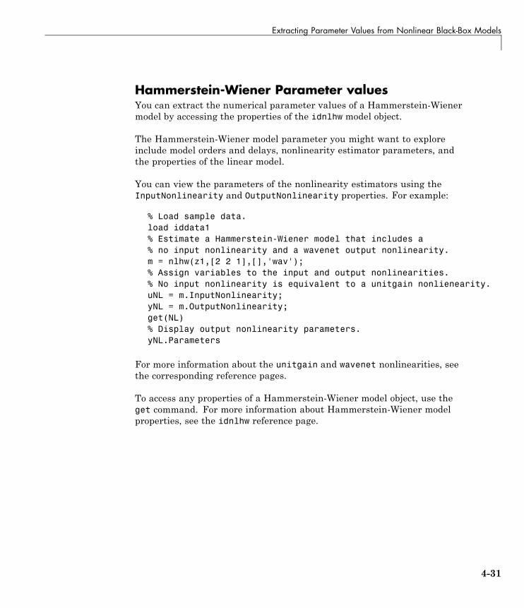
Extracting Parameter Values from Nonlinear Black-Box Models
Hammerstein-Wiener Parameter valuesYou can extract the numerical parameter values of a Hammerstein-Wienermodel by accessing the properties of the idnlhw model object.
The Hammerstein-Wiener model parameter you might want to exploreinclude model orders and delays, nonlinearity estimator parameters, andthe properties of the linear model.
You can view the parameters of the nonlinearity estimators using theInputNonlinearity and OutputNonlinearity properties. For example:
% Load sample data.load iddata1% Estimate a Hammerstein-Wiener model that includes a% no input nonlinearity and a wavenet output nonlinearity.m = nlhw(z1,[2 2 1],[],'wav');% Assign variables to the input and output nonlinearities.% No input nonlinearity is equivalent to a unitgain nonlienearity.uNL = m.InputNonlinearity;yNL = m.OutputNonlinearity;get(NL)% Display output nonlinearity parameters.yNL.Parameters
For more information about the unitgain and wavenet nonlinearities, seethe corresponding reference pages.
To access any properties of a Hammerstein-Wiener model object, use theget command. For more information about Hammerstein-Wiener modelproperties, see the idnlhw reference page.
4-31

4 Nonlinear Black-Box Model Identification
Next Steps After Estimating Nonlinear Black-Box ModelsAfter estimating nonlinear black-box models, you can perform the followingoperations:
• View parameter values, standard deviations of the parameters, lossfunction, and Akaike’s Final Prediction Error (FPE) Criterion at thecommand line using the present command or by get the EstimationInfoproperty of the model.
• Simulate the model using the sim command.
• Predict the model output using the predict command.
• Compute linear approximation of nonlinear ARX and Hammerstein-Wienermodels using linearize or linapp. linearize provides a first-orderTaylor series approximation of the system about an operation point (alsocalled tangent linearization). linapp computes a linear approximation ofa nonlinear model for a given input. For more information about thesecommands, see the “Computing Linear Approximations of NonlinearBlack-Box Models” on page 4-33.
• Import identified models into Simulink software for simulation. For moreinformation, see Chapter 11, “Using System Identification Toolbox Blocks”.
After computing a linear approximation of a nonlinear model, you can performlinear analysis and control design on your model using Control SystemToolbox commands. For more information, see “Using Models with ControlSystem Toolbox Software” on page 10-2.
4-32
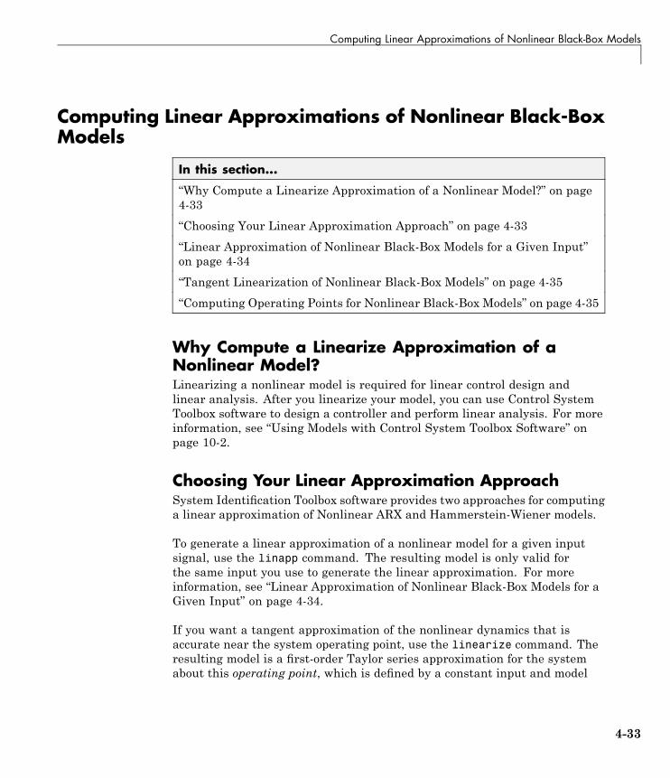
Computing Linear Approximations of Nonlinear Black-Box Models
Computing Linear Approximations of Nonlinear Black-BoxModels
In this section...
“Why Compute a Linearize Approximation of a Nonlinear Model?” on page4-33“Choosing Your Linear Approximation Approach” on page 4-33“Linear Approximation of Nonlinear Black-Box Models for a Given Input”on page 4-34“Tangent Linearization of Nonlinear Black-Box Models” on page 4-35“Computing Operating Points for Nonlinear Black-Box Models” on page 4-35
Why Compute a Linearize Approximation of aNonlinear Model?Linearizing a nonlinear model is required for linear control design andlinear analysis. After you linearize your model, you can use Control SystemToolbox software to design a controller and perform linear analysis. For moreinformation, see “Using Models with Control System Toolbox Software” onpage 10-2.
Choosing Your Linear Approximation ApproachSystem Identification Toolbox software provides two approaches for computinga linear approximation of Nonlinear ARX and Hammerstein-Wiener models.
To generate a linear approximation of a nonlinear model for a given inputsignal, use the linapp command. The resulting model is only valid forthe same input you use to generate the linear approximation. For moreinformation, see “Linear Approximation of Nonlinear Black-Box Models for aGiven Input” on page 4-34.
If you want a tangent approximation of the nonlinear dynamics that isaccurate near the system operating point, use the linearize command. Theresulting model is a first-order Taylor series approximation for the systemabout this operating point, which is defined by a constant input and model
4-33

4 Nonlinear Black-Box Model Identification
state values. For more information, see “Tangent Linearization of NonlinearBlack-Box Models” on page 4-35.
Linear Approximation of Nonlinear Black-BoxModels for a Given Inputlinapp computes the best linear approximation—in a mean-square-errorsense—of a nonlinear ARX or Hammerstein-Wiener model for a given input ora randomly generated input.
linapp estimates the best linear model that is structurally similar to theoriginal nonlinear model and provides the best fit between a given input andthe corresponding simulated response of the nonlinear model.
To compute a linear approximation of a nonlinear black-box model for a giveninput, you must have the following variables in the MATLAB workspace:
• Nonlinear ARX (idnlarx) or Hammerstein-Weiner (idnlhw) model
• Input signal for which you want to obtain a linear approximation, specifiedas a real matrix or an iddata object
You use the specified input signal to compute a linear approximation, asfollows:
• For nonlinear ARX models, linapp estimates a linear ARX model using thesame model orders na, nb, and nk as the original model.
• For Hammerstein-Wiener models, linapp estimates a linear Output-Error(OE) model using the same model orders nb, nf, and nk.
To compute a linear approximation of a nonlinear black-box model for arandomly generated input, you must also have the minimum and maximumscalar input values for generating white-noise input with a magnitude in thisrectangular range, umin and umax in the MATLAB workspace.
For more information, see the linapp reference page.
The resulting linear model is only valid for the same input signal as you theone you used to generate the linear approximation.
4-34

Computing Linear Approximations of Nonlinear Black-Box Models
Tangent Linearization of Nonlinear Black-Box Modelslinearize computes a first-order Taylor series approximation for nonlinearsystem dynamics about and operating point, which is defined by a constantinput and model state values.
To compute a tangent linear approximation of a nonlinear black-box model,you must have the following variables in the MATLAB workspace:
• Nonlinear ARX (idnlarx) or Hammerstein-Weiner (idnlhw) model.
• Operating point
The resulting linear model is accurate in the local neighborhood of theoperating conditions you used to compute the linear approximation.
To specify a known the operating point for your system, you must specify theconstant input and the states. For more information about state definitionsfor each type of parametric model, see the corresponding reference pages:
• idnlarx (nonlinear ARX models)
• idnlhw (nonlinear Hammerstein-Wiener models)
If you do not know the operating point values for your system, see “ComputingOperating Points for Nonlinear Black-Box Models” on page 4-35. For moreinformation, see the linearize(idnlarx) or linearize(idnlhw) referencepage.
Computing Operating Points for Nonlinear Black-BoxModelsThe linearize command for computing a first-order Taylor seriesapproximation for the system requires that you specify an operating point. Anoperating point is defined by a constant input and model state values.
If you do not know the operating conditions of your system, you can use thefindop command to compute the operating point from specifications, asfollows:
• “Computing Operating Point from Steady-State Specifications” on page 4-36
4-35

4 Nonlinear Black-Box Model Identification
• “Computing Operating Points at a Simulation Snapshot” on page 4-36
Computing Operating Point from Steady-State SpecificationsYou can compute an operating point from steady-state specifications, asfollows:
• Using values of input and output signals.If either the steady-state input or output value is unknown, you can specifyit as NaN to estimate this value. This is especially useful when modelingMIMO systems, where only a subset of the input and output steady-statevalues are known.
• Using more complex steady-state specifications.
You construct an object to store the specifications for computing theoperating point, including input and output bounds, known values,and initial guesses. For more information, see operspec(idnlarx) oroperspec(idnlhw).
For more information, see the findop(idnlarx) or findop(idnlhw) referencepage.
Computing Operating Points at a Simulation SnapshotYou can compute an operating point at a specific time during the modelsimulation (snapshot). You must specify the snapshot time and the inputvalue for which you want to compute the operating point. If you do not knowthe equilibrium values of states, you can compute them using an input levelthat causes the output level to reach a steady-state after a finite time.
If your system is at steady state and you are working with linear orHammerstein-Wiener models, you do not need to specify the initial statesbecause they do not affect the steady-state values. For nonlinear ARX models,there can be multiple steady states and you should generally specify theinitial states because they can affect steady-state values. By default, initialstates are set to zero.
However, if your system has not reached steady state at the snapshot time,you must specify the initial states. If you do not know the initial states, you
4-36

Computing Linear Approximations of Nonlinear Black-Box Models
can compute them using the findstates command. For more information,see the findstates(idnlarx) or findstates(idnlhw) reference pages.
4-37

4 Nonlinear Black-Box Model Identification
4-38
5
ODE Parameter Estimation(Grey-Box Modeling)
• “Supported Grey-Box Models” on page 5-2
• “Data Supported by Grey-Box Models” on page 5-3
• “Choosing idgrey or idnlgrey Model Object” on page 5-4
• “Estimating Linear Grey-Box Models” on page 5-6
• “Estimating Nonlinear Grey-Box Models” on page 5-16
• “After Estimating Grey-Box Models” on page 5-23

5 ODE Parameter Estimation (Grey-Box Modeling)
Supported Grey-Box ModelsIf you understand the physics of your system and can represent the systemusing ordinary differential or difference equations (ODEs) with unknownparameters, then you can use System Identification Toolbox commands toperform linear or nonlinear grey-box modeling. Grey-box model ODEs specifythe mathematical structure of the model explicitly, including couplingsbetween parameters and known parameter values. Grey-box modeling isuseful when you know the relationships between variables, constraints onmodel behavior, or explicit equations representing system dynamics.
The toolbox supports both continuous-time and discrete-time models.However, because most laws of physics are expressed in continuous time, it iseasier to construct models with physical insight in continuous time, ratherthan in discrete time.
In addition to dynamic input-output models, you can also create time-seriesmodels that have no inputs and static models that have no states.
If it is too difficult to describe your system using known physical laws, you canperform black-box modeling.
You can also use the idss model object to perform structured modelestimation by using structure matrices As, Bs, Cs, Ds, X0s, Ks to fix or freespecific parameters. However, you cannot use this approach to estimatearbitrary structures (arbitrary parameterization). For more informationabout structure matrices, see “How to Estimate State-Space Models withStructured Parameterization” on page 3-93.
5-2
Data Supported by Grey-Box Models
Data Supported by Grey-Box ModelsYou can estimate both continuous-time or discrete-time grey-box models fordata with the following characteristics:
• Time-domain or frequency-domain data, including time-series data with noinputs.
Note Nonlinear grey-box models support only time-domain data.
• Single-output or multiple-output data
You must first import your data into the MATLAB workspace. If you areusing the System Identification Tool GUI, then import the data into the GUIto make the data available to the toolbox. However, if you prefer to work atthe command line, then represent your data as an iddata or idfrd object.For more information about preparing data for identification, see Chapter1, “Data Processing”.
5-3

5 ODE Parameter Estimation (Grey-Box Modeling)
Choosing idgrey or idnlgrey Model ObjectGrey-box models require that you specify the structure of the ODE model ina file. You use this file to create the idgrey or idnlgrey model object. Youcan use both the idgrey and the idnlgrey objects to model linear systems.However, you can only represent nonlinear dynamics using the idnlgreymodel object.
The idgrey object requires that you write an M-file to describe the lineardynamics in the state-space form, such that this M-file returns the state-spacematrices as a function of your parameters. For more information, see“Specifying the Linear Grey-Box Model Structure” on page 5-6.
The idnlgrey object requires that you write an M-file or MEX-file to describethe dynamics as a set of first-order differential equations, such that this filereturns the output and state derivatives as a function of time, input, state,and parameter values. For more information, see “Specifying the NonlinearGrey-Box Model Structure” on page 5-17.
The following table compares idgrey and idnlgrey model objects.
Comparison of idgrey and idnlgrey Objects
Settings andOperations
Supported byidgrey?
Supported byidnlgrey?
Set bounds onparameter values.
No Yes
Handle initial statesindividually.
No Yes
Perform linear analysis(e.g., using bode).
Yes No
5-4

Choosing idgrey or idnlgrey Model Object
Comparison of idgrey and idnlgrey Objects (Continued)
Settings andOperations
Supported byidgrey?
Supported byidnlgrey?
Honor stabilityconstraints specified byAlgorithm.Advanced.Threshold.ZstabilityandAlgorithm.Advanced.Threshold.Sstabilitymodel properties
Yes No
Note If you knowthe parameter boundsfor obtaining a stableidnlgrey model, setthese bounds to ensurestability.
Estimate a disturbancemodel
YesThe disturbance modelis represented by K instate-space equations.
No
Optimize estimationresults for simulationor prediction
YesSet theAlgorithm.Focusproperty to'Simulation' or'Prediction'.
NoBecause idnlgreymodels areOutput-Error models,there is no differencebetween simulation andprediction results.
5-5
5 ODE Parameter Estimation (Grey-Box Modeling)
Estimating Linear Grey-Box Models
In this section...
“Specifying the Linear Grey-Box Model Structure” on page 5-6“Example – Representing a Grey-Box Model in an M-File” on page 5-7“Example – Estimating a Continuous-Time Grey-Box Model for HeatDiffusion” on page 5-9“Example – Estimating a Discrete-Time Grey-Box Model withParameterized Disturbance” on page 5-12
Specifying the Linear Grey-Box Model StructureYou can estimate linear discrete-time and continuous-time grey-box modelsfor arbitrary ordinary differential or difference equations using single-outputand multiple-output time-domain data, or output-only time-series data.
You must represent your system equations in state-space form. State-spacemodels use state variables x(t) to describe a system as a set of first-orderdifferential equations, rather than by one or more nth-order differentialequations.
In continuous-time, the state-space description has the following form:
� �x t Fx t Gu t Kw ty t Hx t Du t w tx x
( ) ( ) ( ) ( )( ) ( ) ( ) ( )( )
= + += + +=0 0
The discrete-time state-space model structure is often written in theinnovations form:
x kT T Ax kT Bu kT Ke kTy kT Cx kT Du kT e kTx
( ) ( ) ( ) ( )( ) ( ) ( ) ( )( )
+ = + += + +
=0 xx0
5-6
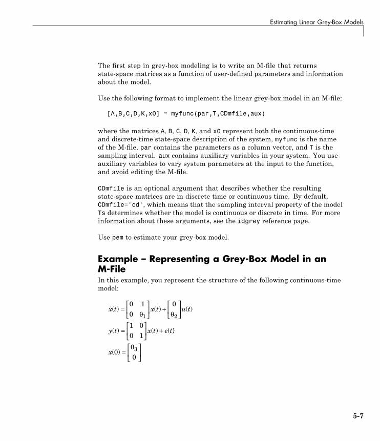
Estimating Linear Grey-Box Models
The first step in grey-box modeling is to write an M-file that returnsstate-space matrices as a function of user-defined parameters and informationabout the model.
Use the following format to implement the linear grey-box model in an M-file:
[A,B,C,D,K,x0] = myfunc(par,T,CDmfile,aux)
where the matrices A, B, C, D, K, and x0 represent both the continuous-timeand discrete-time state-space description of the system, myfunc is the nameof the M-file, par contains the parameters as a column vector, and T is thesampling interval. aux contains auxiliary variables in your system. You useauxiliary variables to vary system parameters at the input to the function,and avoid editing the M-file.
CDmfile is an optional argument that describes whether the resultingstate-space matrices are in discrete time or continuous time. By default,CDmfile='cd', which means that the sampling interval property of the modelTs determines whether the model is continuous or discrete in time. For moreinformation about these arguments, see the idgrey reference page.
Use pem to estimate your grey-box model.
Example – Representing a Grey-Box Model in anM-FileIn this example, you represent the structure of the following continuous-timemodel:
�x t x t u t
y t x t e t
( ) ( ) ( )
( ) ( ) (
=⎡
⎣⎢
⎤
⎦⎥ +
⎡
⎣⎢
⎤
⎦⎥
=⎡
⎣⎢
⎤
⎦⎥ +
0 10
0
1 00 1
1 2θ θ
))
( )x 003=
⎡
⎣⎢
⎤
⎦⎥
θ
5-7
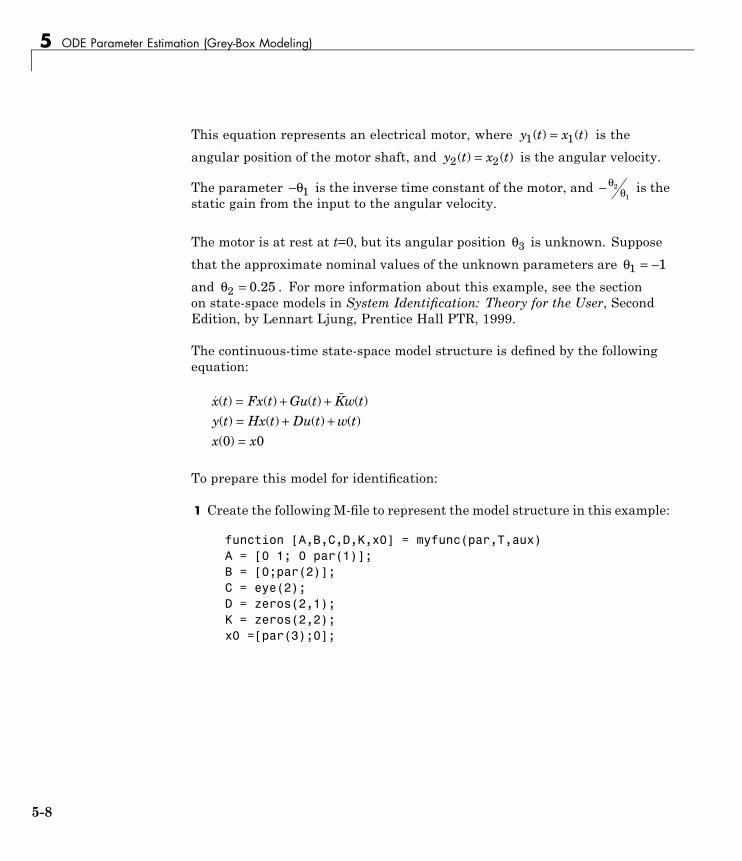
5 ODE Parameter Estimation (Grey-Box Modeling)
This equation represents an electrical motor, where y t x t1 1( ) ( )= is theangular position of the motor shaft, and y t x t2 2( ) ( )= is the angular velocity.
The parameter −θ1 is the inverse time constant of the motor, and −θ θ2
1is the
static gain from the input to the angular velocity.
The motor is at rest at t=0, but its angular position θ3 is unknown. Supposethat the approximate nominal values of the unknown parameters are θ1 1= −
and θ2 0 25= . . For more information about this example, see the sectionon state-space models in System Identification: Theory for the User, SecondEdition, by Lennart Ljung, Prentice Hall PTR, 1999.
The continuous-time state-space model structure is defined by the followingequation:
� �x t Fx t Gu t Kw ty t Hx t Du t w tx x
( ) ( ) ( ) ( )( ) ( ) ( ) ( )( )
= + += + +=0 0
To prepare this model for identification:
1 Create the following M-file to represent the model structure in this example:
function [A,B,C,D,K,x0] = myfunc(par,T,aux)A = [0 1; 0 par(1)];B = [0;par(2)];C = eye(2);D = zeros(2,1);K = zeros(2,2);x0 =[par(3);0];
5-8

Estimating Linear Grey-Box Models
2 Use the following syntax to define an idgrey model object based on themyfunc M-file:
m = idgrey('myfunc',par,'c',T,aux)
where par represents user-defined parameters and contains their nominal(initial) values. 'c' specifies that the underlying parameterization is incontinuous time. aux contains the values of the auxiliary parameters.
Note You must specify T and aux even if they are not used by the myfunccode.
Use pem to estimate the grey-box parameter values:
m = pem(data,m)
where data is the estimation data and m is the idgrey object with unknownparameters.
Note Compare this example to “Example – Estimating StructuredContinuous-Time State-Space Models” on page 3-97, where the same problemis solved using a structured state-space representation.
Example – Estimating a Continuous-Time Grey-BoxModel for Heat DiffusionIn this example, you estimate the heat conductivity and the heat-transfercoefficient of a continuous-time grey-box model for a heated-rod system.
This system consists of a well-insulated metal rod of length L and aheat-diffusion coefficient κ . The input to the system is the heating power u(t)and the measured output y(t) is the temperature at the other end.
5-9
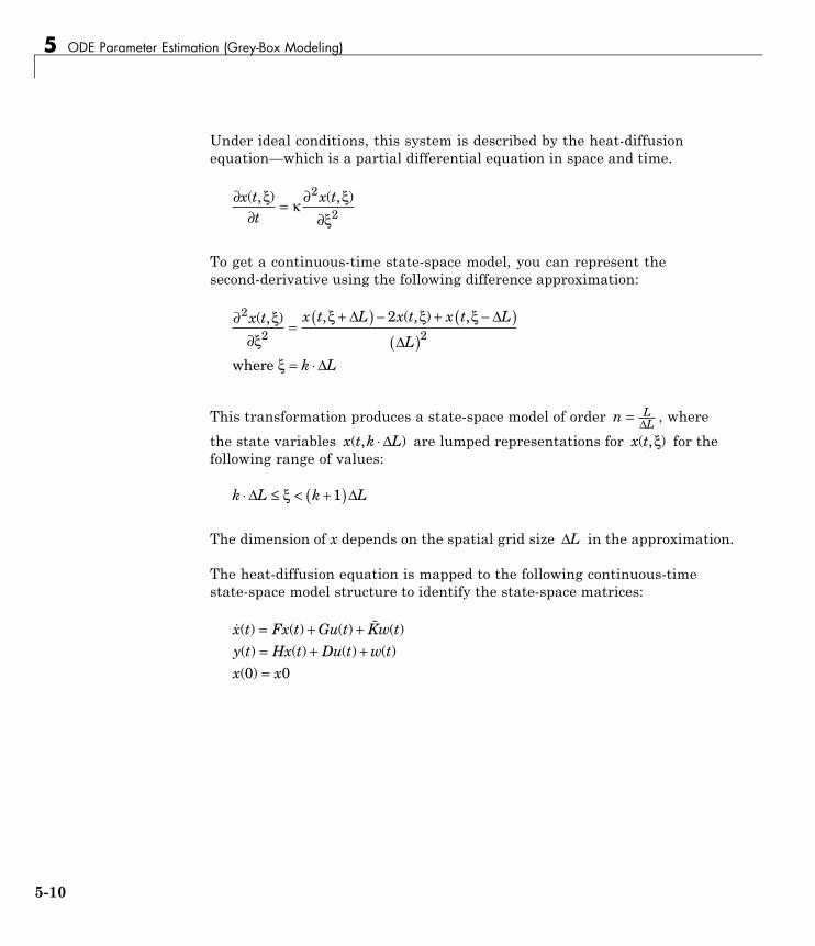
5 ODE Parameter Estimation (Grey-Box Modeling)
Under ideal conditions, this system is described by the heat-diffusionequation—which is a partial differential equation in space and time.
∂∂
= ∂∂
x tt
x t( , ) ( , )ξ κ ξξ
2
2
To get a continuous-time state-space model, you can represent thesecond-derivative using the following difference approximation:
∂∂
=+( ) − + −( )
( )= ⋅
2
2 2
2x t x t L x t x t L
L
k L
( , ) , ( , ) ,ξξ
ξ ξ ξ
ξ
Δ Δ
ΔΔwhere
This transformation produces a state-space model of order n LL= Δ , where
the state variables x t k L( , )⋅ Δ are lumped representations for x t( , )ξ for thefollowing range of values:
k L k L⋅ ≤ < +( )Δ Δξ 1
The dimension of x depends on the spatial grid size ΔL in the approximation.
The heat-diffusion equation is mapped to the following continuous-timestate-space model structure to identify the state-space matrices:
� �x t Fx t Gu t Kw ty t Hx t Du t w tx x
( ) ( ) ( ) ( )( ) ( ) ( ) ( )( )
= + += + +=0 0
5-10

Estimating Linear Grey-Box Models
The following M-file describes the state-space equation for this model. Inthis case, the auxiliary variables specify grid-size variables, so that you canmodify the grid size without the M-file.
function [A,B,C,D,K,x0] = heatd(pars,T,aux)% Number of points in the space-discretizationNgrid = aux(1);% Length of the rodL = aux(2);% Initial rod temperature (uniform)temp = aux(3);% Space intervaldeltaL = L/Ngrid;% Heat-diffusion coefficientkappa = pars(1);% Heat transfer coefficient at far end of rodhtf = pars(2);A = zeros(Ngrid,Ngrid);for kk = 2:Ngrid-1
A(kk,kk-1) = 1;A(kk,kk) = -2;A(kk,kk+1) = 1;
end% Boundary condition on insulated endA(1,1) = -1; A(1,2) = 1;A(Ngrid,Ngrid-1) = 1;A(Ngrid,Ngrid) = -1;A = A*kappa/deltaL/deltaL;B = zeros(Ngrid,1);B(Ngrid,1) = htf/deltaL;C = zeros(1,Ngrid);C(1,1) = 1;D = 0;K = zeros(Ngrid,1);x0 = temp*ones(Ngrid,1);
5-11

5 ODE Parameter Estimation (Grey-Box Modeling)
Use the following syntax to define an idgrey model object based on the heatdM-file:
m = idgrey('heatd',[0.27 1],'c',[10,1,22])
This command specifies the auxiliary parameters as inputs to the function,include the model order 10, the rod length of 1 meter, and an initialtemperature of 22 degrees Celsius. The command also specifies the initialvalues for heat conductivity as 0.27, and for the heat transfer coefficient as 1.
For given data, you can use pem to estimate the grey-box parameter values:
me = pem(data,m)
The following command shows how you can specify to estimate a new modelwith different auxiliary variables directly in the estimator command:
me = pem(data,m,'FileArgument',[20,1,22])
This syntax uses the FileArgument model property to specify a finer gridusing a larger value for Ngrid. For more information about linear grey-boxmodel properties, see the idgrey reference page.
Example – Estimating a Discrete-Time Grey-BoxModel with Parameterized DisturbanceThis example shows how to create a single-input and single-output grey-boxmodel structure when you know the variance of the measurement noise. Thecode in this example uses the Control System Toolbox command kalman forcomputing the Kalman gain from the known and estimated noise variance.
5-12

Estimating Linear Grey-Box Models
Description of the SISO SystemThis example is based on a discrete, single-input and single-output (SISO)system represented by the following state-space equations:
x kT Tpar par
x kT u kT w kT
y kT par
( ) ( ) ( ) ( )
( )
+ =⎡
⎣⎢
⎤
⎦⎥ +
⎡
⎣⎢⎤
⎦⎥ +
=
1 21 0
10
33 4
0 0
par x kT e kT
x x
[ ] +=
( ) ( )
( )
where w and e are independent white-noise terms with covariance matricesR1 and R2, respectively. R1=E{ww’} is a 2–by-2 matrix and R2=E{ee’} is ascalar. par1, par2, par3, and par4 represent the unknown parameter valuesto be estimated.
Assume that you know the variance of the measurement noise R2 to be 1.R1(1,1) is unknown and is treated as an additional parameter par5. Theremaining elements of R1 are known to be zero.
Estimating the Parameters of an idgrey ModelYou can represent the system described in “Description of the SISO System”on page 5-13 as an idgrey (grey-box) model using an M-file. Then, you canuse this M-file and the pem command to estimate the model parameters basedon initial parameter guesses.
To run this example, you must load an input-output data set and representit as an iddata or idfrd object called data. For more information aboutthis operation, see “Representing Time- and Frequency-Domain Data Usingiddata Objects” on page 1-47 or “Representing Frequency-Response DataUsing idfrd Objects” on page 1-67.
To estimate the parameters of a grey-box model:
5-13
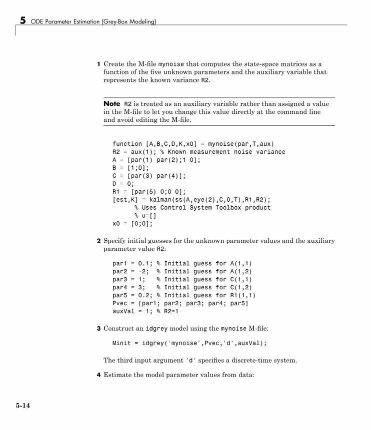
5 ODE Parameter Estimation (Grey-Box Modeling)
1 Create the M-file mynoise that computes the state-space matrices as afunction of the five unknown parameters and the auxiliary variable thatrepresents the known variance R2.
Note R2 is treated as an auxiliary variable rather than assigned a valuein the M-file to let you change this value directly at the command lineand avoid editing the M-file.
function [A,B,C,D,K,x0] = mynoise(par,T,aux)R2 = aux(1); % Known measurement noise varianceA = [par(1) par(2);1 0];B = [1;0];C = [par(3) par(4)];D = 0;R1 = [par(5) 0;0 0];[est,K] = kalman(ss(A,eye(2),C,0,T),R1,R2);
% Uses Control System Toolbox product% u=[]
x0 = [0;0];
2 Specify initial guesses for the unknown parameter values and the auxiliaryparameter value R2:
par1 = 0.1; % Initial guess for A(1,1)par2 = -2; % Initial guess for A(1,2)par3 = 1; % Initial guess for C(1,1)par4 = 3; % Initial guess for C(1,2)par5 = 0.2; % Initial guess for R1(1,1)Pvec = [par1; par2; par3; par4; par5]auxVal = 1; % R2=1
3 Construct an idgrey model using the mynoise M-file:
Minit = idgrey('mynoise',Pvec,'d',auxVal);
The third input argument 'd' specifies a discrete-time system.
4 Estimate the model parameter values from data:
5-14

Estimating Linear Grey-Box Models
Model = pem(data,Minit)
5-15

5 ODE Parameter Estimation (Grey-Box Modeling)
Estimating Nonlinear Grey-Box Models
In this section...
“Supported Nonlinear Grey-Box Models” on page 5-16“Nonlinear Grey-Box Demos and Examples” on page 5-16“Specifying the Nonlinear Grey-Box Model Structure” on page 5-17“Constructing the idnlgrey Object” on page 5-18“Using pem to Estimate Nonlinear Grey-Box Models” on page 5-19“Options for the Estimation Algorithm” on page 5-20
Supported Nonlinear Grey-Box ModelsYou can estimate nonlinear discrete-time and continuous-time grey-boxmodels for arbitrary nonlinear ordinary differential equations usingsingle-output and multiple-output time-domain data, or output-onlytime-series data. Your grey-box models can be static or dynamic.
Grey-box models describe the system behavior as a set of nonlinear ordinarydifferential or difference equations (ODEs) with unknown parameters.
Nonlinear Grey-Box Demos and ExamplesThe System Identification Toolbox product provides several demos and casestudies on creating, manipulating, and estimating nonlinear grey-box models.You can access these demos by typing the following command at the prompt:
iddemo
For examples of M-files and MEX-files that specify model structure, see thetoolbox/ident/iddemos/examples directory. For example, the model of aDC motor—used in the demo idnlgreydemo1—is described in files dcmotor_mand dcmotor_c.
5-16
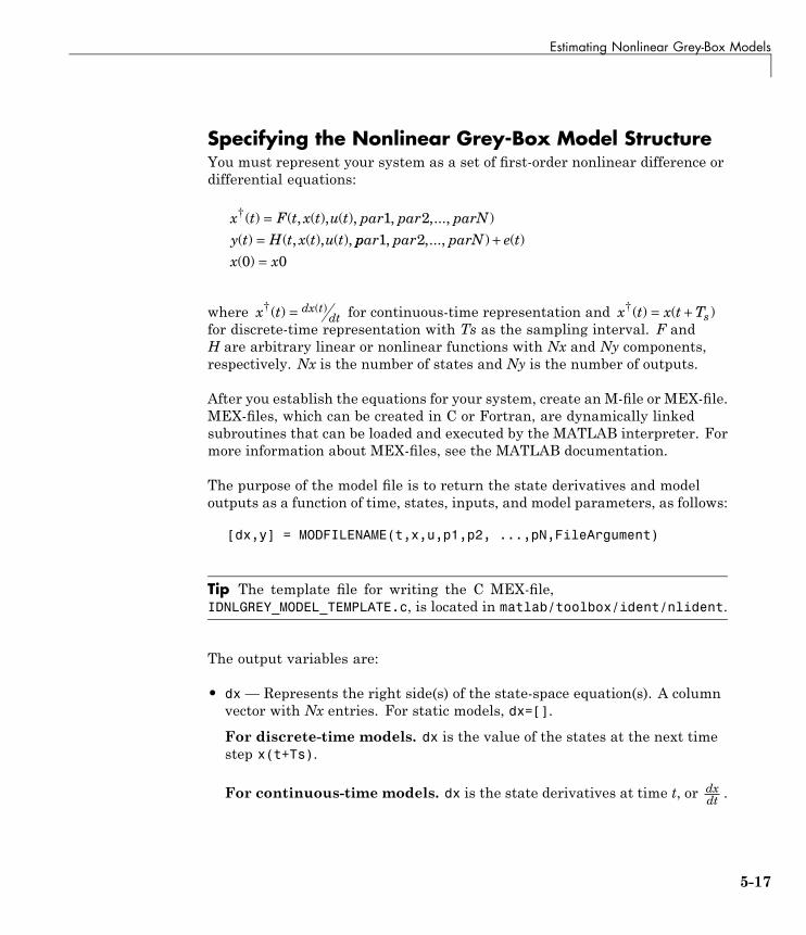
Estimating Nonlinear Grey-Box Models
Specifying the Nonlinear Grey-Box Model StructureYou must represent your system as a set of first-order nonlinear difference ordifferential equations:
x t F t x t u t par par parNy t H t x t u t
†( ) ( , ( ), ( ), , ,..., )( ) ( , ( ), ( ),
==
1 2ppar par parN e t
x x1 2
0 0, ,..., ) ( )
( )+
=
where x t dx tdt
† ( )( ) = for continuous-time representation and x t x t Ts†( ) ( )= +
for discrete-time representation with Ts as the sampling interval. F andH are arbitrary linear or nonlinear functions with Nx and Ny components,respectively. Nx is the number of states and Ny is the number of outputs.
After you establish the equations for your system, create an M-file or MEX-file.MEX-files, which can be created in C or Fortran, are dynamically linkedsubroutines that can be loaded and executed by the MATLAB interpreter. Formore information about MEX-files, see the MATLAB documentation.
The purpose of the model file is to return the state derivatives and modeloutputs as a function of time, states, inputs, and model parameters, as follows:
[dx,y] = MODFILENAME(t,x,u,p1,p2, ...,pN,FileArgument)
Tip The template file for writing the C MEX-file,IDNLGREY_MODEL_TEMPLATE.c, is located in matlab/toolbox/ident/nlident.
The output variables are:
• dx— Represents the right side(s) of the state-space equation(s). A columnvector with Nx entries. For static models, dx=[].
For discrete-time models. dx is the value of the states at the next timestep x(t+Ts).
For continuous-time models. dx is the state derivatives at time t, or dxdt .
5-17

5 ODE Parameter Estimation (Grey-Box Modeling)
• y— Represents the right side(s) of the output equation(s). A column vectorwith Ny entries.
The file inputs are:
• t — Current time.
• x — State vector at time t. For static models, equals [].
• u— Input vector at time t. For time-series models, equals [].
• p1,p2, ...,pN— Parameters, which can be real scalars, column vectorsor two-dimensional matrices. N is the number of parameter objects. Forscalar parameters, N is the total number of parameter elements.
• FileArgument— Contains auxiliary variables that might be required forupdating the constants in the state equations.
Tip After creating a model file, call it directly from the MATLAB softwarewith reasonable inputs and verify the output values.
For an example of creating grey-box model files and idnlgrey model object,see the demo Creating idnlgrey Model Files.
Constructing the idnlgrey ObjectAfter you create the M-file or MEX-file with your model structure, you mustdefine an idnlgrey object. This object shares many of the properties of thelinear idgrey model object.
Use the following syntax to define the idnlgrey model object:
m = idnlgrey('filename',Order,Parameters,InitialStates)
The idnlgrey arguments are defined as follows:
• 'filename'— Name of the M-file or MEX-file storing the model structure.This file must be on the MATLAB path when you use this model object formodel estimation, prediction, or simulation.
5-18
Estimating Nonlinear Grey-Box Models
• Order— Vector with three entries [Ny Nu Nx], specifying the number ofmodel outputs Ny, the number of inputs Nu, and the number of states Nx.
• Parameters — Parameters, specified as struct arrays, cell arrays, ordouble arrays.
• InitialStates— Specified in the same way as parameters. Must be thefourth input to the idnlgrey constructor.
For detailed information about this object and its properties, see the idnlgreyreference page.
Use pem to estimate your grey-box model.
Using pem to Estimate Nonlinear Grey-Box ModelsYou can use the pem command to estimate the unknown idnlgrey modelparameters and initial states using measured data.
The input-output dimensions of the data must be compatible with the inputand output orders you specified for the idnlgrey model.
Use the following general estimation syntax:
m = pem(data,m)
where data is the estimation data and m is the idnlgrey model object youconstructed.
You can pass additional property-value pairs to pem to specify the propertiesof the model or the estimation algorithm. Assignable properties includethe ones returned by the get(idnlgrey) command and the algorithmproperties returned by the get(idnlgrey, 'Algorithm'), such as MaxIterand Tolerance. For detailed information about these model properties, seethe idnlgrey reference page.
For more information about validating your models, see Chapter 8, “ModelAnalysis”.
5-19

5 ODE Parameter Estimation (Grey-Box Modeling)
Options for the Estimation AlgorithmThe Algorithm property of the model specifies the estimation algorithm,which simulates the model several times by trying various parameter valuesto reduce the prediction error.
The following algorithm properties can affect the quality of the results:
• “Simulation Method” on page 5-20
• “Search Method” on page 5-20
• “Gradient Options” on page 5-21
• “Example – Specifying Algorithm Properties” on page 5-21
For detailed information about these and other model properties, see theidnlgrey reference page.
Simulation MethodYou can specify the simulation method using the SimulationOptions(struct) fields of the model Algorithm property.
System Identification Toolbox software provides several variable-step andfixed-step solvers for simulating idnlgrey models. To view a list of availablesolvers and their properties, type the following command at the prompt:
idprops idnlgrey algorithm.simulationoptions
For discrete-time systems, the default solver is 'FixedStepDiscrete'. Forcontinuous-time systems, the default solver is 'ode45'.
By default, SimulationOptions.Solver is set to 'Auto', which automaticallyselects either 'ode45' or 'FixedStepDiscrete' during estimation andsimulation—depending on whether the system is continuous or discrete intime.
Search MethodYou can specify the search method for estimating model parameters using theSearchMethod field of the Algorithm property. Two categories of methods areavailable for nonlinear grey-box modeling.
5-20

Estimating Nonlinear Grey-Box Models
One category of methods consists of the minimization schemes that arebased on line-search methods, including Gauss-Newton type methods,steepest-descent methods, and Levenberg-Marquardt methods.
The Trust-Region Reflective Newton method of nonlinear least-squares(lsqnonlin), where the cost is the sum of squares of errors between themeasured and simulated outputs, requires Optimization Toolbox™ software.When the parameter bounds differ from the default +/- Inf, this searchmethod handles the bounds better than the schemes based on a line search.However, unlike the line-search-based methods, lsqnonlin only works withCriterion='Trace'.
By default, SearchMethod is set to Auto, which automatically selects amethod from the available minimizers. If the Optimization Toolbox product isinstalled, SearchMethod is set to 'lsqnonlin'. Otherwise, SearchMethod is acombination of line-search based schemes.
Gradient OptionsYou can specify the method for calculating gradients using theGradientOptions field of the Algorithm property. Gradients are thederivatives of errors with respect to unknown parameters and initial states.
Gradients are calculated by numerically perturbing unknown quantities andmeasuring their effects on the simulation error.
Option for gradient computation include the choice of the differencing scheme(forward, backward or central), the size of minimum perturbation of theunknown quantities, and whether the gradients are calculated simultaneouslyor individually.
Example – Specifying Algorithm PropertiesYou can specify the Algorithm fields directly in the estimation syntax, asproperty-value pairs.
For example, you can specify the following properties as part of the pem syntax:
m = pem(data,init_model,'Search','gn',...'MaxIter',5,...'Display','On')
5-21

5 ODE Parameter Estimation (Grey-Box Modeling)
5-22

After Estimating Grey-Box Models
After Estimating Grey-Box ModelsAfter estimating linear and nonlinear grey-box models, you can simulate themodel output using the sim command. For more information, see Chapter 9,“Simulation and Prediction”.
The toolbox represents linear grey-box models using the idgrey model object.To convert grey-box models to state-space form, use the idss command,as described in “Transforming Between Linear Model Representations” onpage 3-117. You can then analyze the model behavior using transient- andfrequency-response plots and other linear analysis plots.
The toolbox represents nonlinear grey-box models as idnlgrey model objects.These model objects store the parameter values resulting from the estimation.You can access these parameters from the model objects to use these variablesin computation in the MATLAB workspace.
Note Linearization of nonlinear grey-box models is not supported.
You can import grey box models into a Simulink model using the SystemIdentification Toolbox Block Library. For more information, see “SimulatingModel Output” on page 11-6.
5-23

5 ODE Parameter Estimation (Grey-Box Modeling)
5-24
6
Time Series ModelIdentification
• “What Are Time-Series Models?” on page 6-2
• “Preparing Time-Series Data” on page 6-3
• “Estimating Time-Series Power Spectra” on page 6-4
• “Estimating AR and ARMA Models” on page 6-7
• “Estimating State-Space Time-Series Models” on page 6-12
• “Example – Identifying Time-Series Models at the Command Line” on page6-14
• “Estimating Nonlinear Models for Time-Series Data” on page 6-15

6 Time Series Model Identification
What Are Time-Series Models?A time series is one or more measured output channels with no measuredinput.
You can estimate time-series spectra using both time- and frequency-domaindata. Time-series spectra describe time-series variations using cycliccomponents at different frequencies.
You can also estimate parametric autoregressive (AR), autoregressive andmoving average (ARMA), and state-space time-series models. For a definitionof these models, see “Definition of AR and ARMA Models” on page 6-7.
Note ARMA and state-space models are supported for time-domain dataonly. Only single-output ARMA models are supported.
6-2

Preparing Time-Series Data
Preparing Time-Series DataBefore you can estimate models for time-series data, you must import yourdata into the MATLAB software. You can estimate models from eithertime-domain and frequency-domain data. For information about whichvariables you need to represent time-series data, see “Importing Time-SeriesData into MATLAB” on page 1-7.
For more information about preparing data for modeling, see “Ways to ProcessData for System Identification” on page 1-2.
If your data is already in the MATLAB workspace, you can import it directlyinto the System Identification Tool GUI. If you prefer to work at the commandline, you must represent the data as a System Identification Toolbox dataobject instead.
In the System Identification Tool GUI. When you import scalar ormultiple-output time series data into the GUI, leave the Input field empty.For more information about importing data, see “Representing Data in theGUI” on page 1-13.
At the command line. To represent a time series vector or a matrix s as aniddata object, use the following syntax:
y = iddata(s,[],Ts);
s contains as many columns as there are measured outputs. For time-domaindata, set Ts to the sampling interval. For continuous-time frequency domaindata, set Ts to 0.
6-3
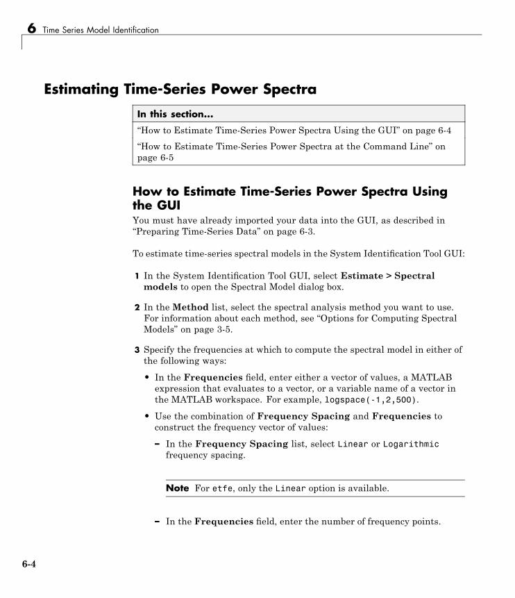
6 Time Series Model Identification
Estimating Time-Series Power Spectra
In this section...
“How to Estimate Time-Series Power Spectra Using the GUI” on page 6-4“How to Estimate Time-Series Power Spectra at the Command Line” onpage 6-5
How to Estimate Time-Series Power Spectra Usingthe GUIYou must have already imported your data into the GUI, as described in“Preparing Time-Series Data” on page 6-3.
To estimate time-series spectral models in the System Identification Tool GUI:
1 In the System Identification Tool GUI, select Estimate > Spectralmodels to open the Spectral Model dialog box.
2 In the Method list, select the spectral analysis method you want to use.For information about each method, see “Options for Computing SpectralModels” on page 3-5.
3 Specify the frequencies at which to compute the spectral model in either ofthe following ways:
• In the Frequencies field, enter either a vector of values, a MATLABexpression that evaluates to a vector, or a variable name of a vector inthe MATLAB workspace. For example, logspace(-1,2,500).
• Use the combination of Frequency Spacing and Frequencies toconstruct the frequency vector of values:
– In the Frequency Spacing list, select Linear or Logarithmicfrequency spacing.
Note For etfe, only the Linear option is available.
– In the Frequencies field, enter the number of frequency points.
6-4

Estimating Time-Series Power Spectra
For time-domain data, the frequency ranges from 0 to the Nyquistfrequency. For frequency-domain data, the frequency ranges from thesmallest to the largest frequency in the data set.
4 In the Frequency Resolution field, enter the frequency resolution, asdescribed in “Options for Frequency Resolution” on page 3-6. To use thedefault value, enter default or leave the field empty.
5 In theModel Name field, enter the name of the correlation analysis model.The model name should be unique in the Model Board.
6 Click Estimate to add this model to the Model Board in the SystemIdentification Tool GUI.
7 In the Spectral Model dialog box, click Close.
8 To view the estimated disturbance spectrum, select the Noise spectrumcheck box in the System Identification Tool GUI. For more informationabout working with this plot, see “Creating Noise-Spectrum Plots” on page8-40.
To export the model to the MATLAB workspace, drag it to the To Workspacerectangle in the System Identification Tool GUI. You can view the powerspectrum and the confidence intervals of the resulting idfrd model objectusing the bode command.
How to Estimate Time-Series Power Spectra at theCommand LineYou can use the etfe, spa, and spafdr commands to estimate power spectraof time series for both time-domain and frequency-domain data. The followingtable provides a brief description of each command.
You must have already prepared your data, as described in “PreparingTime-Series Data” on page 6-3.
The resulting models are stored as an idfrd model object, which containsSpectrumData and its variance. For multiple-output data, SpectrumDatacontains power spectra of each output and the cross-spectra between eachoutput pair.
6-5

6 Time Series Model Identification
Estimating Frequency Response of Time Series
Command Description
etfe Estimates a periodogram using Fourieranalysis.
spa Estimates the power spectrum with itsstandard deviation using spectral analysis.
spafdr Estimates the power spectrum withits standard deviation using a variablefrequency resolution.
For example, suppose y is time-series data. The following commands estimatethe power spectrum g and the periodogram p, and plot both models with threestandard deviation confidence intervals:
g = spa(y)p = etfe(y)bode(g,p,'sd',3)
For detailed information about these commands, see the correspondingreference pages.
6-6

Estimating AR and ARMA Models
Estimating AR and ARMA Models
In this section...
“Definition of AR and ARMA Models” on page 6-7“Estimating Polynomial Time-Series Models in the GUI” on page 6-7“Estimating AR and ARMA Models at the Command Line” on page 6-10
Definition of AR and ARMA ModelsFor a single-output signal y(t), the AR model is given by the following equation:
A q y t e t( ) ( ) ( )=
The AR model is a special case of the ARX model with no input.
The ARMA model for a single-output time-series is given by the followingequation:
A q y t C q e t( ) ( ) ( ) ( )=
The ARMA structure reduces to the AR structure for C(q)=1. The ARMAmodel is a special case of the ARMAX model with no input.
For more information about polynomial models, see “What Are Black-BoxPolynomial Models?” on page 3-41.
Estimating Polynomial Time-Series Models in the GUIBefore you begin, you must have accomplished the following:
• Prepared the data, as described in “Preparing Time-Series Data” on page6-3
• Estimated model order, as described in “Preliminary Step – EstimatingModel Orders and Input Delays” on page 3-49
6-7

6 Time Series Model Identification
• (Multiple-output AR models only) Specified the model-order matrix inthe MATLAB workspace before estimation, as described in “Options forMultiple-Input and Multiple-Output ARX Orders” on page 3-64
To estimate AR and ARMA models using the System Identification Tool GUI:
1 In the System Identification Tool GUI, select Estimate > Linearparametric models to open the Linear Parametric Models dialog box.
2 In the Structure list, select the polynomial model structure you want toestimate from the following options:
• AR:[na]
• ARMA:[na nc]
This action updates the options in the Linear Parametric Models dialog boxto correspond with this model structure. For information about each modelstructure, see “Definition of AR and ARMA Models” on page 6-7.
Note OE and BJ structures are not available for time-series models.
3 In the Orders field, specify the model orders, as follows:
• For single-output models. Enter the model orders according to thesequence displayed in the Structure field.
• For multiple-output ARX models. (AR models only) Enter themodel orders directly, as described in “Options for Multiple-Input andMultiple-Output ARX Orders” on page 3-64. Alternatively, enter thename of the matrix NA in the MATLAB Workspace browser that storesmodel orders, which is Ny-by-Ny.
Tip To enter model orders and delays using the Order Editor dialog box,click Order Editor.
6-8

Estimating AR and ARMA Models
4 (AR models only) Select the estimation Method as ARX or IV(instrumental variable method). For more information about thesemethods, see “Algorithms for Estimating Polynomial Models” on page 3-66.
Note IV is not available for multiple-output data.
5 In the Name field, edit the name of the model or keep the default. Thename of the model should be unique in the Model Board.
6 In the Initial state list, specify how you want the algorithm to treat initialstates. For more information about the available options, see “Options forInitial States” on page 3-66.
Tip If you get an inaccurate fit, try setting a specific method for handlinginitial states rather than choosing it automatically.
7 In the Covariance list, select Estimate if you want the algorithm tocompute parameter uncertainties. Effects of such uncertainties aredisplayed on plots as model confidence regions.
To omit estimating uncertainty, select None. Skipping uncertaintycomputation might reduce computation time for complex models and largedata sets.
8 (ARMA only) To view the estimation progress at the command line, selectthe Trace check box. During estimation, the following information isdisplayed for each iteration:
• Loss function — Equals the determinant of the estimated covariancematrix of the input noise.
• Parameter values — Values of the model structure coefficients youspecified.
• Search direction — Changes in parameter values from the previousiteration.
6-9

6 Time Series Model Identification
• Fit improvements — Shows the actual versus expected improvements inthe fit.
9 Click Estimate to add this model to the Model Board in the SystemIdentification Tool GUI.
10 (Prediction-error method only) To stop the search and save the resultsafter the current iteration has been completed, click Stop Iterations. Tocontinue iterations from the current model, click the Continue iter buttonto assign current parameter values as initial guesses for the next search.
11 To plot the model, select the appropriate check box in the Model Viewsarea of the System Identification Tool GUI. For more information aboutvalidating models, see Chapter 8, “Model Analysis”.
You can export the model to the MATLAB workspace for further analysisby dragging it to the To Workspace rectangle in the System IdentificationTool GUI.
Estimating AR and ARMA Models at the CommandLineYou can estimate AR and ARMA models at the command line. Forsingle-output time-series, the resulting models are idpoly model objects. Formultiple-output time-series, the resulting models are idarx model objects.For more information about models objects, see “Creating Model Structures atthe Command Line” on page 2-11.
The following table summarizes the commands and specifies whethersingle-output or multiple-output models are supported.
Commands for Estimating Polynomial Time-Series Models
Method Name Description Supported Data
ar Noniterative, least-squares methodto estimate linear, discrete-timesingle-output AR models.
Time-domain, time-series iddatadata object.
6-10
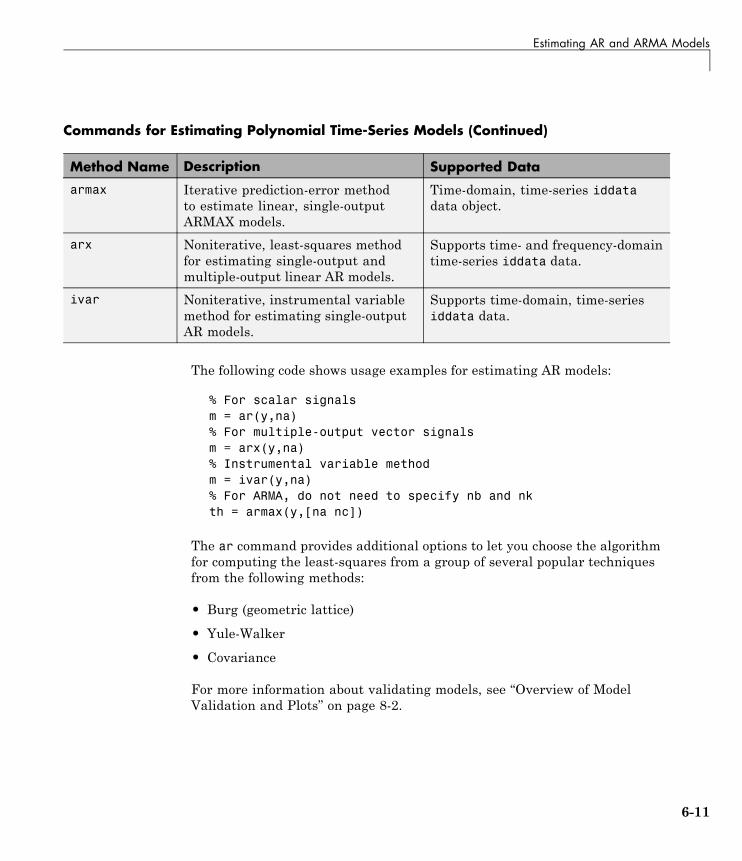
Estimating AR and ARMA Models
Commands for Estimating Polynomial Time-Series Models (Continued)
Method Name Description Supported Data
armax Iterative prediction-error methodto estimate linear, single-outputARMAX models.
Time-domain, time-series iddatadata object.
arx Noniterative, least-squares methodfor estimating single-output andmultiple-output linear AR models.
Supports time- and frequency-domaintime-series iddata data.
ivar Noniterative, instrumental variablemethod for estimating single-outputAR models.
Supports time-domain, time-seriesiddata data.
The following code shows usage examples for estimating AR models:
% For scalar signalsm = ar(y,na)% For multiple-output vector signalsm = arx(y,na)% Instrumental variable methodm = ivar(y,na)% For ARMA, do not need to specify nb and nkth = armax(y,[na nc])
The ar command provides additional options to let you choose the algorithmfor computing the least-squares from a group of several popular techniquesfrom the following methods:
• Burg (geometric lattice)
• Yule-Walker
• Covariance
For more information about validating models, see “Overview of ModelValidation and Plots” on page 8-2.
6-11

6 Time Series Model Identification
Estimating State-Space Time-Series Models
In this section...
“Definition of State-Space Time-Series Model” on page 6-12“Estimating State-Space Models at the Command Line” on page 6-12
Definition of State-Space Time-Series ModelThe discrete-time state-space model for a time series is given by the followingequations:
x kT T Ax kT Ke kTy kT Cx kT e kT( ) ( ) ( )( ) ( ) ( )
+ = += +
where T is the sampling interval and y(kT) is the output at time instant kT.
The time-series structure corresponds to the general structure with empty Band D matrices.
For information about general discrete-time and continuous-time structuresfor state-space models, see “What Are State-Space Models?” on page 3-73.
Estimating State-Space Models at the Command LineYou can estimate single-output and multiple-output state-space models at thecommand line for time-domain and frequency-domain data (iddata object).
The following table provides a brief description of each command. Theresulting models are idss model objects.
6-12
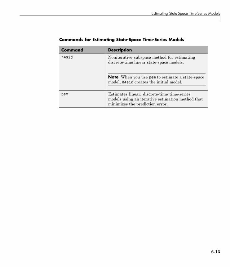
Estimating State-Space Time-Series Models
Commands for Estimating State-Space Time-Series Models
Command Description
n4sid Noniterative subspace method for estimatingdiscrete-time linear state-space models.
Note When you use pem to estimate a state-spacemodel, n4sid creates the initial model.
pem Estimates linear, discrete-time time-seriesmodels using an iterative estimation method thatminimizes the prediction error.
6-13

6 Time Series Model Identification
Example – Identifying Time-Series Models at the CommandLine
The following example simulates a time-series model, compares spectralestimates, covariance estimates, and predicts output of the model:
ts0 = idpoly([1 -1.5 0.7],[]);ir = sim(ts0,[1;zeros(24,1)]);% Define the true covariance functionRy0 = conv(ir,ir(25:-1:1));e = idinput(200,'rgs');% Define y vectory = sim(ts0,e);% iddata object with sampling time 1y = iddata(y)plot(y)per = etfe(y);speh = spa(y);ffplot(per,speh,ts0)% Estimate a second-order AR modelts2 = ar(y,2);ffplot(speh,ts2,ts0,'sd',3)% Get covariance function estimatesRyh = covf(y,25);Ryh = [Ryh(end:-1:2),Ryh]';ir2 = sim(ts2,[1;zeros(24,1)]);Ry2 = conv(ir2,ir2(25:-1:1));plot([-24:24]'*ones(1,3),[Ryh,Ry2,Ry0])% The prediction ability of the modelcompare(y,ts2,5)
6-14

Estimating Nonlinear Models for Time-Series Data
Estimating Nonlinear Models for Time-Series DataWhen a linear model provides an insufficient description of the dynamics, youcan try estimating a nonlinear models. To learn more about when to estimatenonlinear models, see “When to Identify Linear Versus Nonlinear Models” inthe Getting Started Guide.
Before you can estimate models for time-series data, you must have alreadyprepared the data as described in “Preparing Time-Series Data” on page 6-3.
For black-box modeling of time-series data, the toolbox supports nonlinearARX models. To learn how to estimate this type of model, see “IdentifyingNonlinear ARX Models” on page 4-4.
If you understand the underlying physics of the system, you can specify anordinary differential or difference equation and estimate the coefficients. Tolearn how to estimate this type of model, see “Estimating Nonlinear Grey-BoxModels” on page 5-16.
For more information about validating models, see “Overview of ModelValidation and Plots” on page 8-2.
6-15

6 Time Series Model Identification
6-16

7
Recursive Techniques forModel Identification
• “What Is Recursive Estimation?” on page 7-2
• “Commands for Recursive Estimation” on page 7-3
• “Algorithms for Recursive Estimation” on page 7-6
• “Data Segmentation” on page 7-14
7 Recursive Techniques for Model Identification
What Is Recursive Estimation?Many real-world applications, such as adaptive control, adaptive filtering, andadaptive prediction, require a model of the system to be available online whilethe system is in operation. Estimating models for batches of input-outputdata is useful for addressing the following types of questions regardingsystem operation:
• Which input should be applied at the next sampling instant?
• How should the parameters of a matched filter be tuned?
• What are the predictions of the next few outputs?
• Has a failure occurred? If so, what type of failure?
You might also use online models to investigate time variations in systemand signal properties.
The methods for computing online models are called recursive identificationmethods. Recursive algorithms are also called recursive parameter estimation,adaptive parameter estimation, sequential estimation, and online algorithms.
For examples of recursive estimation and data segmentation, run theRecursive Estimation and Data Segmentation demo by typing the followingcommand at the prompt:
iddemo5
For detailed information about recursive parameter estimation algorithms,see the corresponding chapter in System Identification: Theory for the User byLennart Ljung (Prentice Hall PTR, Upper Saddle River, NJ, 1999).
7-2

Commands for Recursive Estimation
Commands for Recursive EstimationYou can recursively estimate linear polynomial models, such as ARX,ARMAX, Box-Jenkins, and Output-Error models. If you are working withtime-series data that contains no inputs and a single output, you canestimate AR (Auto-Regressive) and ARMA (Auto-Regressive Moving Average)single-output models.
Before estimating models using recursive algorithms, you must import yourdata into the MATLAB workspace and represent your data in either of thefollowing formats:
• Matrix of the form [y u]. y represents the output data using one or morecolumn vectors. Similarly, u represents the input data using one or morecolumn vectors.
• iddata or idfrd object. For more information about creating these objects,see Chapter 1, “Data Processing”.
The general syntax for recursive estimation commands is as follows:
[params,y_hat]=command(data,nn,adm,adg)
params matrix contains the values of the estimated parameters, where thekth row contains the parameters associated with time k, which are computedusing the data values in the rows up to and including the row k.
y_hat contains the predicted output values such that the kth row of y_hat iscomputed based on the data values in the rows up to and including the row k.
Tip y_hat contains the adaptive predictions of the output and is useful foradaptive filtering applications, such as noise cancelation.
nn specified the model orders and delay according to the specific polynomialstructure of the model. For example, nn=[na nb nk] for ARX models. Formore information about specifying polynomial model orders and delays, see“Identifying Input-Output Polynomial Models” on page 3-41.
7-3

7 Recursive Techniques for Model Identification
adm and adg specify any of the four recursive algorithm, as described in“Algorithms for Recursive Estimation” on page 7-6.
The following table summarizes the recursive estimation commandssupported by the System Identification Toolbox product. The commanddescription indicates whether you can estimate single-input, single-output,multiple-input, and multiple-output, and time-series (no input) models. Fordetails about each command, see the corresponding reference page.
Tip For ARX and AR models, use rarx. For single-input/single-outputARMAX or ARMA, Box-Jenkins, and Output-Error models, use rarmax, rbj,and roe, respectively.
Commands for Linear Recursive Estimation
Command Description
rarmax Estimate parameters ofsingle-input/single-output ARMAXand ARMA models.
rarx Estimate parameters of single- ormultiple-input and single-output ARXand AR models. Does not supportmultiple-output system.
rbj Estimate parameters ofsingle-input/single-output Box-Jenkinsmodels.
roe Estimate parameters ofsingle-input/single-output Output-Errormodels.
7-4

Commands for Recursive Estimation
Commands for Linear Recursive Estimation (Continued)
Command Description
rpem Estimate parameters of multiple-inputand single-output ARMAX/ARMA,Box-Jenkins, or Output-Error modelsusing the general recursive prediction-erroralgorithm for estimating the parametergradient.
Note Unlike pem, rpem does not supportstate-space models.
rplr Use as an alternative to rpem to estimateparameters of multiple-input andsingle-output systems when you wantto use recursive pseudolinear regressionmethod.
7-5
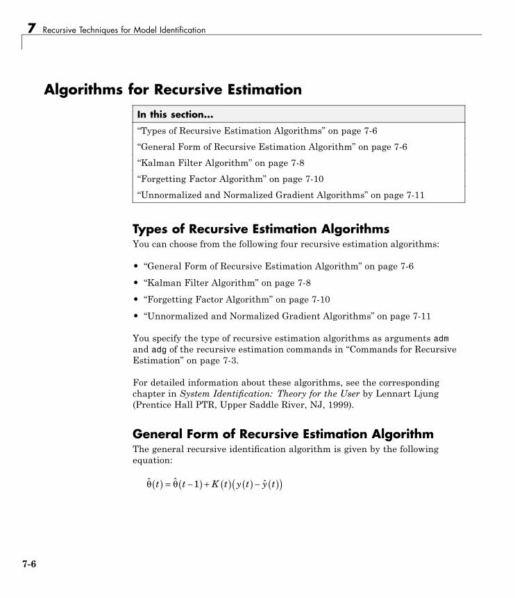
7 Recursive Techniques for Model Identification
Algorithms for Recursive Estimation
In this section...
“Types of Recursive Estimation Algorithms” on page 7-6“General Form of Recursive Estimation Algorithm” on page 7-6“Kalman Filter Algorithm” on page 7-8“Forgetting Factor Algorithm” on page 7-10“Unnormalized and Normalized Gradient Algorithms” on page 7-11
Types of Recursive Estimation AlgorithmsYou can choose from the following four recursive estimation algorithms:
• “General Form of Recursive Estimation Algorithm” on page 7-6
• “Kalman Filter Algorithm” on page 7-8
• “Forgetting Factor Algorithm” on page 7-10
• “Unnormalized and Normalized Gradient Algorithms” on page 7-11
You specify the type of recursive estimation algorithms as arguments admand adg of the recursive estimation commands in “Commands for RecursiveEstimation” on page 7-3.
For detailed information about these algorithms, see the correspondingchapter in System Identification: Theory for the User by Lennart Ljung(Prentice Hall PTR, Upper Saddle River, NJ, 1999).
General Form of Recursive Estimation AlgorithmThe general recursive identification algorithm is given by the followingequation:
ˆ ˆ ˆθ θt t K t y t y t( ) = −( ) + ( ) ( ) − ( )( )1
7-6

Algorithms for Recursive Estimation
θ t( ) is the parameter estimate at time t. y(t) is the observed output at time tand y t( ) is the prediction of y(t) based on observations up to time t-1. Thegain, K(t), determines how much the current prediction error y t y t( ) − ( )ˆaffects the update of the parameter estimate. The estimation algorithms
minimize the prediction-error term y t y t( ) − ( )ˆ .
The gain has the following general form:
K t Q t t( ) = ( ) ( )ψ
The recursive algorithms supported by the System Identification Toolboxproduct differ based on different approaches for choosing the form of Q(t) and
computing ψ t( ) , where ψ t( ) represents the gradient of the predicted modeloutput ˆ |y t θ( ) with respect to the parameters θ .
The simplest way to visualize the role of the gradient ψ t( ) of the parameters,is to consider models with a linear-regression form:
y t t t e tT( ) = ( ) ( ) + ( )ψ θ0
In this equation, ψ t( ) is the regression vector that is computed based onprevious values of measured inputs and outputs. θ0 t( ) represents the trueparameters. e(t) is the noise source (innovations), which is assumed to be
white noise. The specific form of ψ t( ) depends on the structure of thepolynomial model.
For linear regression equations, the predicted output is given by the followingequation:
ˆ ˆy t t tT( ) = ( ) −( )ψ θ 1
7-7
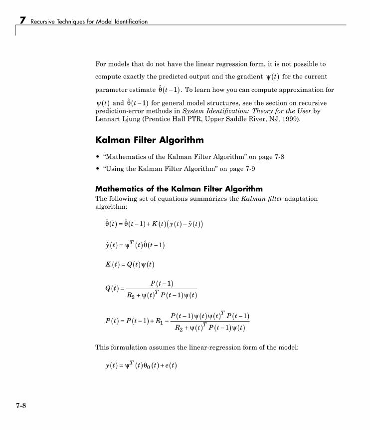
7 Recursive Techniques for Model Identification
For models that do not have the linear regression form, it is not possible to
compute exactly the predicted output and the gradient ψ t( ) for the currentparameter estimate θ t −( )1 . To learn how you can compute approximation for
ψ t( ) and θ t −( )1 for general model structures, see the section on recursiveprediction-error methods in System Identification: Theory for the User byLennart Ljung (Prentice Hall PTR, Upper Saddle River, NJ, 1999).
Kalman Filter Algorithm
• “Mathematics of the Kalman Filter Algorithm” on page 7-8
• “Using the Kalman Filter Algorithm” on page 7-9
Mathematics of the Kalman Filter AlgorithmThe following set of equations summarizes the Kalman filter adaptationalgorithm:
ˆ ˆ ˆθ θt t K t y t y t( ) = −( ) + ( ) ( ) − ( )( )1
ˆ ˆy t t tT( ) = ( ) −( )ψ θ 1
K t Q t t( ) = ( ) ( )ψ
Q tP t
R t P t tT( ) = −( )+ ( ) −( ) ( )
1
12 ψ ψ
P t P t RP t t t P t
R t P t t
T
T( ) = −( ) + −−( ) ( ) ( ) −( )+ ( ) −( ) ( )
11 1
11
2
ψ ψ
ψ ψ
This formulation assumes the linear-regression form of the model:
y t t t e tT( ) = ( ) ( ) + ( )ψ θ0
7-8

Algorithms for Recursive Estimation
The Kalman filter is used to obtain Q(t).
This formulation also assumes that the true parameters θ0 t( ) are describedby a random walk:
θ θ0 0 1t t w t( ) = −( ) + ( )
w(t) is Gaussian white noise with the following covariance matrix, or driftmatrix R1:
Ew t w t RT( ) ( ) = 1
R2 is the variance of the innovations e(t) in the following equation:
y t t t e tT( ) = ( ) ( ) + ( )ψ θ0
The Kalman filter algorithm is entirely specified by the sequence of data y(t),
the gradient ψ t( ) , R1, R2, and the initial conditions θ t =( )0 (initial guess of
the parameters) and P t =( )0 (covariance matrix that indicates parameterserrors).
Note To simplify the inputs, you can scale R1, R2, and P t =( )0 of theoriginal problem by the same value such that R2 is equal to 1. This scalingdoes not affect the parameters estimates.
Using the Kalman Filter AlgorithmThe general syntax for the command described in “Algorithms for RecursiveEstimation” on page 7-6 is the following:
[params,y_hat]=command(data,nn,adm,adg)
7-9

7 Recursive Techniques for Model Identification
To specify the Kalman filter algorithm, set adm to 'kf' and adg to the valueof the drift matrix R1 (described in “Mathematics of the Kalman FilterAlgorithm” on page 7-8).
Forgetting Factor Algorithm
• “Mathematics of the Forgetting Factor Algorithm” on page 7-10
• “Using the Forgetting Factor Algorithm” on page 7-11
Mathematics of the Forgetting Factor AlgorithmThe following set of equations summarizes the forgetting factor adaptationalgorithm:
ˆ ˆ ˆθ θt t K t y t y t( ) = −( ) + ( ) ( ) − ( )( )1
ˆ ˆy t t tT( ) = ( ) −( )ψ θ 1
K t Q t t( ) = ( ) ( )ψ
Q t P tP t
t P t tT( ) = ( ) = −( )+ ( ) −( ) ( )
1
1λ ψ ψ
P t P tP t t t P t
t P t t
T
T( ) = −( ) − −( ) ( ) ( ) −( )+ ( ) −( ) ( )
⎛
⎝⎜⎜
⎞
⎠
1 11 1
1λψ ψ
λ ψ ψ⎟⎟⎟
To obtain Q(t), the following function is minimized at time t:
λt kkt
e k−=∑ ( )21
This approach discounts old measurements exponentially such that an
observation that is τ samples old carries a weight that is equal to λτ times
the weight of the most recent observation. τ λ= −1
1 represents the memory
7-10

Algorithms for Recursive Estimation
horizon of this algorithm. Measurements older than τ λ= −1
1 typically carry aweight that is less than about 0.3.
λ is called the forgetting factor and typically has a positive value between0.97 and 0.995.
Note In the linear regression case, the forgetting factor algorithm isknown as the recursive least-squares (RLS) algorithm. The forgetting factoralgorithm for λ = 1 is equivalent to the Kalman filter algorithm with R1=0and R2=1. For more information about the Kalman filter algorithm, see“Kalman Filter Algorithm” on page 7-8.
Using the Forgetting Factor AlgorithmThe general syntax for the command described in “Algorithms for RecursiveEstimation” on page 7-6 is the following:
[params,y_hat]=command(data,nn,adm,adg)
To specify the forgetting factor algorithm, set adm to 'ff' and adg to thevalue of the forgetting factor λ (described in “Mathematics of the ForgettingFactor Algorithm” on page 7-10).
Tip λ typically has a positive value from 0.97 to 0.995.
Unnormalized and Normalized Gradient Algorithms
• “Mathematics of the Unnormalized and Normalized Gradient Algorithm”on page 7-12
• “Using the Unnormalized and Normalized Gradient Algorithms” on page7-12
7-11

7 Recursive Techniques for Model Identification
Mathematics of the Unnormalized and Normalized GradientAlgorithmIn the linear regression case, the gradient methods are also known as theleast mean squares (LMS) methods.
The following set of equations summarizes the unnormalized gradient andnormalized gradient adaptation algorithm:
ˆ ˆ ˆθ θt t K t y t y t( ) = −( ) + ( ) ( ) − ( )( )1
ˆ ˆy t t tT( ) = ( ) −( )ψ θ 1
K t Q t t( ) = ( ) ( )ψ
In the unnormalized gradient approach, Q(t) is the product of the gain γand the identity matrix:
Q t I( ) = γ
In the normalized gradient approach, Q(t) is the product of the gain γ , and
the identity matrix is normalized by the magnitude of the gradient ψ t( ) :
Q tt
I( ) =( )γ
ψ 2
These choices of Q(t) update the parameters in the negative gradient direction,where the gradient is computed with respect to the parameters.
Using the Unnormalized and Normalized Gradient AlgorithmsThe general syntax for the command described in “Algorithms for RecursiveEstimation” on page 7-6 is the following:
[params,y_hat]=command(data,nn,adm,adg)
7-12

Algorithms for Recursive Estimation
To specify the unnormalized gain algorithm, set adm to 'ug' and adg to thevalue of the gain γ (described in “Mathematics of the Unnormalized andNormalized Gradient Algorithm” on page 7-12).
To specify the normalized gain algorithm, set adm to 'ng' and adg to thevalue of the gain γ .
7-13
7 Recursive Techniques for Model Identification
Data SegmentationFor systems that exhibit abrupt changes while the data is being collected,you might want to develop models for separate data segments such that thesystem does not change during a particular data segment. Such modelingrequires identification of the time instants when the changes occur in thesystem, breaking up the data into segments according to these time instants,and identification of models for the different data segments.
The following cases are typical applications for data segmentation:
• Segmentation of speech signals, where each data segment correspondsto a phonem.
• Detection of trend breaks in time series.
• Failure detection, where the data segments correspond to operation withand without failure.
• Estimating different working modes of a system.
Use segment to build polynomial models, such as ARX, ARMAX, AR, andARMA, so that the model parameters are piece-wise constant over time. Fordetailed information about this command, see the corresponding referencepage.
To see an example of using data segmentation, run the Recursive Estimationand Data Segmentation demonstration by typing to the following command atthe prompt:
iddemo5
7-14

8
Model Analysis
• “Overview of Model Validation and Plots” on page 8-2
• “Using Model Output Plots to Validate and Compare Models” on page 8-8
• “Using Residual Analysis Plots to Validate Models” on page 8-16
• “Using Impulse- and Step-Response Plots to Validate Models” on page 8-24
• “Using Frequency-Response Plots to Validate Models” on page 8-32
• “Creating Noise-Spectrum Plots” on page 8-40
• “Using Pole-Zero Plots to Validate Models” on page 8-47
• “Using Nonlinear ARX Plots to Validate Models” on page 8-52
• “Using Hammerstein-Wiener Plots to Validate Models” on page 8-56
• “Using Akaike’s Criteria to Validate Models” on page 8-61
• “Computing Model Uncertainty” on page 8-64
• “Troubleshooting Models” on page 8-67
• “Next Steps After Getting an Accurate Model” on page 8-72

8 Model Analysis
Overview of Model Validation and Plots
In this section...
“When to Validate Models” on page 8-2“Ways to Validate Models” on page 8-2“Data for Validating Models” on page 8-4“Supported Model Plots” on page 8-4“Plotting Models in the GUI” on page 8-5“Getting Advice About Models” on page 8-7
When to Validate ModelsAfter estimating each model, you can validate whether the model reproducessystem behavior within acceptable bounds. You iterate between estimationand validation until you find the simplest model that best captures the systemdynamics.
For ideas on how to adjust your modeling strategy based on validation results,see “Troubleshooting Models” on page 8-67.
Tip If you have installed the Control System Toolbox product, you can alsoview models using the LTI Viewer. For more information, see “Viewing ModelResponse Using the LTI Viewer” on page 10-5.
Ways to Validate ModelsYou can use the following approaches to validate models:
• Comparing simulated or predicted model output to measured output.
See “Using Model Output Plots to Validate and Compare Models” on page8-8.
• Analyzing autocorrelation and cross-correlation of the residuals with input.
See “Using Residual Analysis Plots to Validate Models” on page 8-16.
8-2
Overview of Model Validation and Plots
• Analyzing model response. For more information, see the following:
- “Using Impulse- and Step-Response Plots to Validate Models” on page8-24
- “Using Frequency-Response Plots to Validate Models” on page 8-32
For information about the response of the noise model, see “CreatingNoise-Spectrum Plots” on page 8-40.
• Plotting the poles and zeros of the linear parametric model.
For more information, see “Using Pole-Zero Plots to Validate Models” onpage 8-47.
• Comparing the response of nonparametric models, such as impulse-, step-,and frequency-response models, to parametric models, such as linearpolynomial models, state-space model, and nonlinear parametric models.
Note Do not use this comparison when feedback is present in the systembecause feedback makes nonparametric models unreliable. To test iffeedback is present in the system, use the advice command on the data.
• Compare models using Akaike Information Criterion or Akaike FinalPrediction Error.
For more information, see the aic and fpe reference page.
• Plotting linear and nonlinear blocks of Hammerstein-Wiener and nonlinearARX models.
For more information, see “Using Hammerstein-Wiener Plots to ValidateModels” on page 8-56 and “Using Nonlinear ARX Plots to Validate Models”on page 8-52.
Displaying confidence intervals on supported plots helps you assess theuncertainty of model parameters. For more information, see “ComputingModel Uncertainty” on page 8-64.
8-3
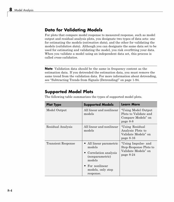
8 Model Analysis
Data for Validating ModelsFor plots that compare model response to measured response, such as modeloutput and residual analysis plots, you designate two types of data sets: onefor estimating the models (estimation data), and the other for validating themodels (validation data). Although you can designate the same data set to beused for estimating and validating the model, you risk overfitting your data.When you validate a model using an independent data set, this process iscalled cross-validation.
Note Validation data should be the same in frequency content as theestimation data. If you detrended the estimation data, you must remove thesame trend from the validation data. For more information about detrending,see “Subtracting Trends from Signals (Detrending)” on page 1-94.
Supported Model PlotsThe following table summarizes the types of supported model plots.
Plot Type Supported Models Learn More
Model Output All linear and nonlinearmodels
“Using Model OutputPlots to Validate andCompare Models” onpage 8-8
Residual Analysis All linear and nonlinearmodels
“Using ResidualAnalysis Plots toValidate Models” onpage 8-16
Transient Response • All linear parametricmodels
• Correlation analysis(nonparametric)models
• For nonlinearmodels, only stepresponse.
“Using Impulse- andStep-Response Plots toValidate Models” onpage 8-24
8-4

Overview of Model Validation and Plots
Plot Type Supported Models Learn More
Frequency Response • All linear parametricmodels
• Spectral analysis(nonparametric)models
“UsingFrequency-ResponsePlots to ValidateModels” on page 8-32
Noise Spectrum • All linear parametricmodels
• Spectral analysis(nonparametric)models
“CreatingNoise-Spectrum Plots”on page 8-40
Poles and Zeros All linear parametricmodels
“Using Pole-Zero Plotsto Validate Models” onpage 8-47
Nonlinear ARX Nonlinear ARX modelsonly
“Using NonlinearARX Plots to ValidateModels” on page 8-52
Hammerstein-Wiener Hammerstein-Wienermodels only
“UsingHammerstein-WienerPlots to ValidateModels” on page 8-56
Plotting Models in the GUITo create one or more plots of your models, select the corresponding check boxin the Model Views area of the System Identification Tool GUI. An activemodel icon has a thick line in the icon, while an inactive model has a thin line.Only active models appear on the selected plots.
To include or exclude a model on a plot, click the corresponding icon in theSystem Identification Tool GUI. Clicking the model icon updates any plotsthat are currently open.
8-5

8 Model Analysis
For example, in the following figure,Model output is selected. In this case,the models n4s4 is not included on the plot because only arx441 is active.
'��%�����
*����%�����
,�������������������������%�����&
Plots Include Only Active Models
To close a plot, clear the corresponding check box in the System IdentificationTool GUI.
Tip To get information about a specific plot, select a help topic from the Helpmenu in the plot window.
For general information about working with plots in the System IdentificationToolbox product , see “Working with Plots in the System Identification ToolGUI” on page 12-15.
8-6

Overview of Model Validation and Plots
Getting Advice About ModelsUse the advice command on an estimated model to answer the followingquestions about the model:
• Should I increase or decrease the model order?
• Should I estimate a noise model?
• Is feedback present?
8-7

8 Model Analysis
Using Model Output Plots to Validate and Compare Models
In this section...
“Supported Model Types” on page 8-8“What Does a Model Output Plot Show?” on page 8-8“Choosing Simulated or Predicted Output” on page 8-9“How to Plot Model Output Using the GUI” on page 8-11“Displaying the Confidence Interval” on page 8-13“How to Plot and Compare Model Output at the Command Line” on page8-14
Supported Model TypesYou can validate linear parametric models and nonlinear models by checkinghow well the simulated or predicted output of the model matches themeasured output.
Note For nonparametric models, including impulse-response, step-response,and frequency-response models, model output plots are not available. Fortime-series models, you can only generate model-output plots for parametricmodels using time-domain time-series (no input) measured data.
What Does a Model Output Plot Show?The model output plot shows different information depending on the domainof the input-output validation data, as follows:
• For time-domain validation data, the plot shows simulated or predictedmodel output.
• For frequency-domain data, the plot shows the simulated complex-valuedamplitude of the model output. The complex-valued amplitude is equal tothe product of the Fourier transform of the input and the model frequencyfunction.
8-8

Using Model Output Plots to Validate and Compare Models
• For frequency-response data, the plot shows the simulated amplitude of themodel frequency response.
For linear models, you can estimate a model using time-domain data, andthen validate the model using frequency domain data. For nonlinear models,you can only use time-domain data for both estimation and validation.
The following figure shows a sample Model Output plot, created in the SystemIdentification Tool GUI.
Choosing Simulated or Predicted OutputHow you validate the model output should match how you plan to use themodel. If you plan to use the model for simulation applications, validate themodel by comparing simulated output to the validation data. Using a modelfor prediction is common in controls applications where you want to predictoutput for a specific number of steps in advance. For example, if you aremodeling a plant for a control system, your model must perform for predictionover a horizon that corresponds to the time-constant of the system.
8-9

8 Model Analysis
The main difference between simulation and prediction is whether the toolboxuses measured or computed previous outputs for computing the next output.
Note Output-error models, obtained by fixing K to zero for state-spacemodels and setting na=nc=nd=0 for polynomial models, do not use pastoutputs. Therefore, for these models, the simulated and the predicted outputsare the same for any value of k.
Simulating a model means that you compute the response of a model toa particular input. Then, the toolbox feeds this computed output into thedifferential (continuous-time) or difference (discrete-time) equation forcalculating the next output value. In this way, the simulation progressesusing previously calculated outputs in the difference equation to producethe next output; with an infinite prediction horizon (k=∞), the simulationhas no limit on how far out in time it computes output values. Simulatingmodels uses the input-data values from the validation data set to computethe output values.
Simulating models uses only past input values to compute the output values.If the model-output expression includes past outputs, the toolbox computesthe first output value using the initial conditions and the inputs. Then, thetoolbox feeds this computed output into the difference equation or differentialequation for calculating the next output value. Thus, no past outputs are usedin the computation of output at the current time.
Simulation always uses a discrete model and continuous-time models arediscretized for simulation purposes. Simulation does not involve the noisemodel unless you explicitly specify to compute the response to the noise sourceinput. During simulation, the toolbox computes the first output value usingthe initial conditions and the inputs.
Predicting future outputs of a model from previous data over a time horizon ofk samples or kTs time units—where Ts is the sampling interval and k is theprediction horizon—requires both past inputs and past outputs.
During prediction, the algorithm uses both the measured and the calculatedoutput data values in the difference equation for computing the next output.The predicted value y(t) is computed from all available inputs u(s), where
8-10
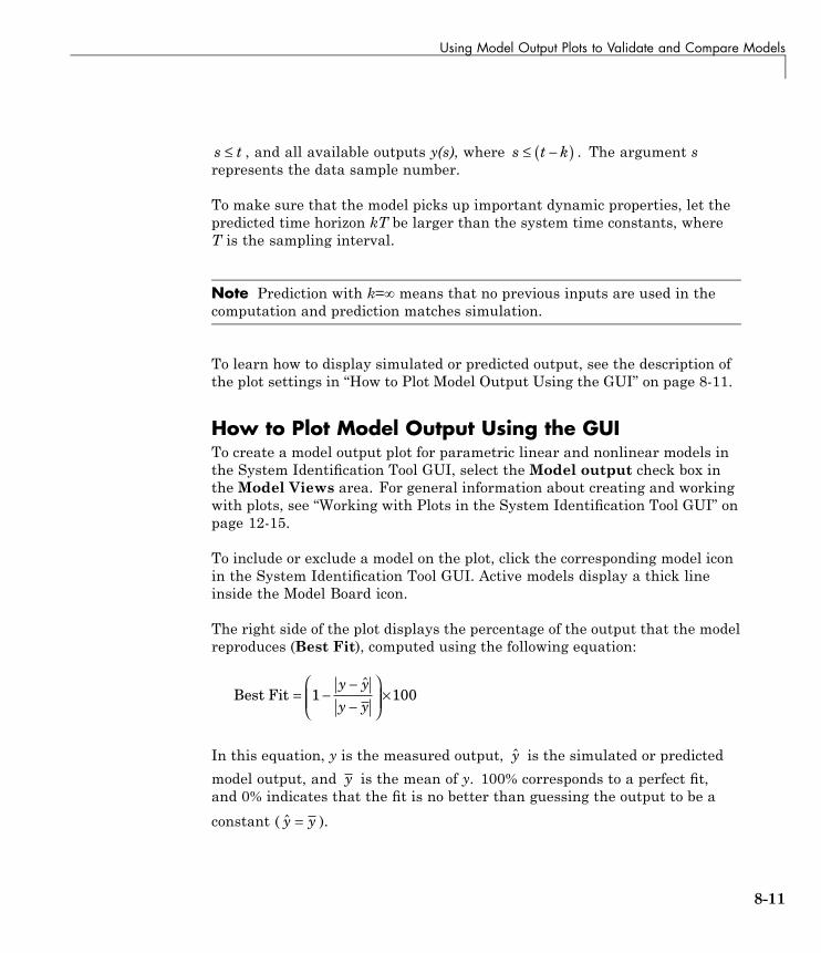
Using Model Output Plots to Validate and Compare Models
s t≤ , and all available outputs y(s), where s t k≤ −( ) . The argument srepresents the data sample number.
To make sure that the model picks up important dynamic properties, let thepredicted time horizon kT be larger than the system time constants, whereT is the sampling interval.
Note Prediction with k=∞ means that no previous inputs are used in thecomputation and prediction matches simulation.
To learn how to display simulated or predicted output, see the description ofthe plot settings in “How to Plot Model Output Using the GUI” on page 8-11.
How to Plot Model Output Using the GUITo create a model output plot for parametric linear and nonlinear models inthe System Identification Tool GUI, select the Model output check box intheModel Views area. For general information about creating and workingwith plots, see “Working with Plots in the System Identification Tool GUI” onpage 12-15.
To include or exclude a model on the plot, click the corresponding model iconin the System Identification Tool GUI. Active models display a thick lineinside the Model Board icon.
The right side of the plot displays the percentage of the output that the modelreproduces (Best Fit), computed using the following equation:
Best Fit = −−−
⎛
⎝⎜⎜
⎞
⎠⎟⎟ ×1 100
y y
y y
ˆ
In this equation, y is the measured output, y is the simulated or predictedmodel output, and y is the mean of y. 100% corresponds to a perfect fit,and 0% indicates that the fit is no better than guessing the output to be aconstant ( y y= ).
8-11

8 Model Analysis
Because of the definition of Best Fit, it is possible for this value to be negative.A negative best fit is worse than 0% and can occur for the following reasons:
• The estimation algorithm failed to converge.
• The model was not estimated by minimizing y y− ˆ . Best Fit canbe negative when you minimized 1-step-ahead prediction during theestimation, but validate using the simulated output y .
• The validation data set was not preprocessed in the same way as theestimation data set.
The following table summarizes the Model Output plot settings.
Model Output Plot Settings
Action Command
Display confidence intervals.
Note Confidence intervals are onlyavailable for simulated model outputof linear models. Confidence internalare not available for nonlinear ARXand Hammerstein-Wiener models.
• To display the dashed lines oneither side of the nominal modelcurve, select Options > Showconfidence intervals. Selectthis option again to hide theconfidence intervals.
• To change the confidencevalue, select Options > Set %confidence level, and choose avalue from the list.
• To enter your own confidencelevel, select Options > Setconfidence level > Other.Enter the value as a probability(between 0 and 1) or as thenumber of standard deviations ofa Gaussian distribution.
8-12

Using Model Output Plots to Validate and Compare Models
Model Output Plot Settings (Continued)
Action Command
Change between simulated outputor predicted output.
Note Prediction is only availablefor time-domain validation data.
• Select Options > Simulatedoutput or Options > k stepahead predicted output.
• To change the prediction horizon,select Options > Set predictionhorizon, and select the numberof samples.
• To enter your own predictionhorizon, select Options > Setprediction horizon > Other.Enter the value in terms of thenumber of samples.
Display the actual output values(Signal plot), or the differencebetween model output and measuredoutput (Error plot).
Select Options > Signal plot orOptions > Error plot.
(Time-domain validation data only)Set the time range for model outputand the time interval for which theBest Fit value is computed.
SelectOptions > Customized timespan for fit and enter the minimumand maximum time values. Forexample:
[1 20]
(Multiple-output system only)Select a different output.
Select the output by name in theChannel menu.
Displaying the Confidence IntervalIn the GUI, you can display a confidence interval on the plot to gain insightinto the quality of a linear model. To learn how to show or hide confidenceinterval, see the description of the plot settings in “How to Plot Model OutputUsing the GUI” on page 8-11.
The confidence interval corresponds to the range of output values with aspecific probability of being the actual output of the system. The toolbox uses
8-13
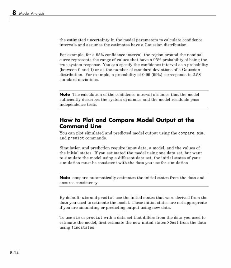
8 Model Analysis
the estimated uncertainty in the model parameters to calculate confidenceintervals and assumes the estimates have a Gaussian distribution.
For example, for a 95% confidence interval, the region around the nominalcurve represents the range of values that have a 95% probability of being thetrue system response. You can specify the confidence interval as a probability(between 0 and 1) or as the number of standard deviations of a Gaussiandistribution. For example, a probability of 0.99 (99%) corresponds to 2.58standard deviations.
Note The calculation of the confidence interval assumes that the modelsufficiently describes the system dynamics and the model residuals passindependence tests.
How to Plot and Compare Model Output at theCommand LineYou can plot simulated and predicted model output using the compare, sim,and predict commands.
Simulation and prediction require input data, a model, and the values ofthe initial states. If you estimated the model using one data set, but wantto simulate the model using a different data set, the initial states of yoursimulation must be consistent with the data you use for simulation.
Note compare automatically estimates the initial states from the data andensures consistency.
By default, sim and predict use the initial states that were derived from thedata you used to estimate the model. These initial states are not appropriateif you are simulating or predicting output using new data.
To use sim or predict with a data set that differs from the data you used toestimate the model, first estimate the new initial states X0est from the datausing findstates:
8-14

Using Model Output Plots to Validate and Compare Models
X0est=findstates(model,data)
Next, specify the estimated initial states X0est as an argument in sim orpredict. For example:
y=sim(model,data,'InitialState',X0est)
Command Description Example
compare Plots simulated orpredicted modeloutput on top of themeasured output.You should usean independentvalidation data setas input to the model.
To plot five-step-aheadpredicted output of the modelmod against the validationdata data, use the followingcommand:
compare(data,mod,5)
Note Omitting the thirdargument assumes aninfinite horizon and results insimulation.
sim Plots simulated modeloutput only.
To simulate the response ofthe model model using inputdata data, use the followingcommand:
sim(model,data)
predict Plots predicted modeloutput only.
To perform one-step-aheadprediction of the response forthe model model and inputdata data, use the followingcommand:
predict(model,data,1)
8-15

8 Model Analysis
Using Residual Analysis Plots to Validate Models
In this section...
“What Is Residual Analysis?” on page 8-16“Supported Model Types” on page 8-17“What Does the Residuals Plot Show?” on page 8-17“Displaying the Confidence Interval” on page 8-18“How to Plot Residuals Using the GUI” on page 8-19“How to Plot Residuals at the Command Line” on page 8-21“Example – Examining Model Residuals” on page 8-21
What Is Residual Analysis?Residuals are differences between the one-step-predicted output from themodel and the measured output from the validation data set. Thus, residualsrepresent the portion of the validation data not explained by the model.
Residual analysis consists of two tests: the whiteness test and theindependence test.
According to the whiteness test criteria, a good model has the residualautocorrelation function inside the confidence interval of the correspondingestimates, indicating that the residuals are uncorrelated.
According to the independence test criteria, a good model has residualsuncorrelated with past inputs. Evidence of correlation indicates that themodel does not describe how part of the output relates to the correspondinginput. For example, a peak outside the confidence interval for lag k meansthat the output y(t) that originates from the input u(t-k) is not properlydescribed by the model.
Your model should pass both the whiteness and the independence tests,except in the following cases:
8-16
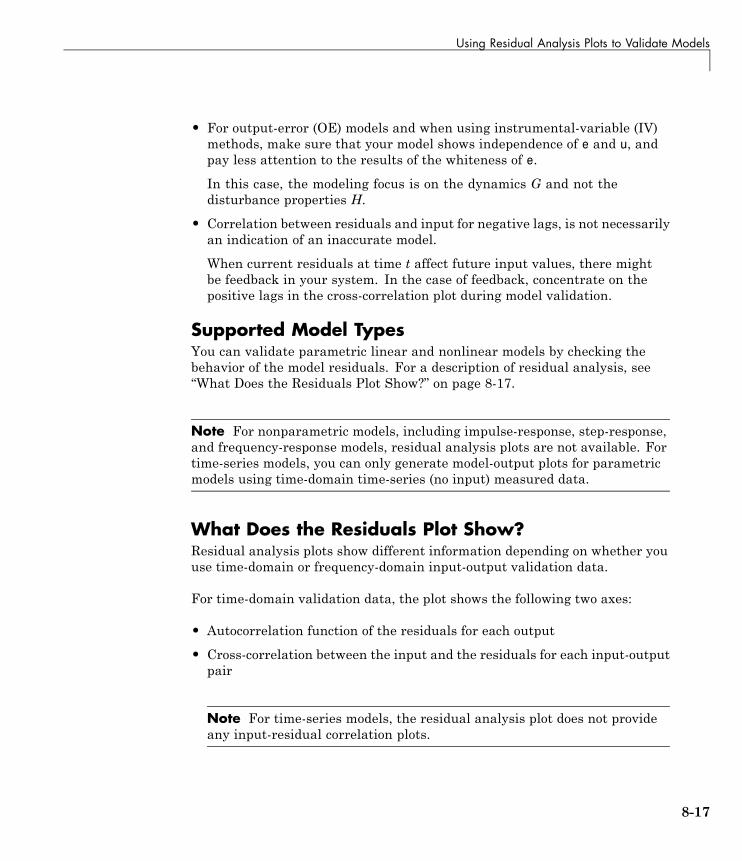
Using Residual Analysis Plots to Validate Models
• For output-error (OE) models and when using instrumental-variable (IV)methods, make sure that your model shows independence of e and u, andpay less attention to the results of the whiteness of e.
In this case, the modeling focus is on the dynamics G and not thedisturbance properties H.
• Correlation between residuals and input for negative lags, is not necessarilyan indication of an inaccurate model.
When current residuals at time t affect future input values, there mightbe feedback in your system. In the case of feedback, concentrate on thepositive lags in the cross-correlation plot during model validation.
Supported Model TypesYou can validate parametric linear and nonlinear models by checking thebehavior of the model residuals. For a description of residual analysis, see“What Does the Residuals Plot Show?” on page 8-17.
Note For nonparametric models, including impulse-response, step-response,and frequency-response models, residual analysis plots are not available. Fortime-series models, you can only generate model-output plots for parametricmodels using time-domain time-series (no input) measured data.
What Does the Residuals Plot Show?Residual analysis plots show different information depending on whether youuse time-domain or frequency-domain input-output validation data.
For time-domain validation data, the plot shows the following two axes:
• Autocorrelation function of the residuals for each output
• Cross-correlation between the input and the residuals for each input-outputpair
Note For time-series models, the residual analysis plot does not provideany input-residual correlation plots.
8-17

8 Model Analysis
For frequency-domain validation data, the plot shows the following two axes:
• Estimated power spectrum of the residuals for each output
• Transfer-function amplitude from the input to the residuals for eachinput-output pair
For linear models, you can estimate a model using time-domain data, andthen validate the model using frequency domain data. For nonlinear models,the System Identification Toolbox product supports only time-domain data.
The following figure shows a sample Residual Analysis plot, created in theSystem Identification Tool GUI.
Displaying the Confidence IntervalYou can display a confidence interval on the plot in the GUI to gain insightinto the quality of the model. To learn how to show or hide confidenceinterval, see the description of the plot settings in “How to Plot ResidualsUsing the GUI” on page 8-19.
8-18
Using Residual Analysis Plots to Validate Models
Note If you are working in the System Identification Tool GUI, you canspecify a custom confidence interval. If you are using the resid command, theconfidence interface is fixed at 99%.
The confidence interval corresponds to the range of residual values with aspecific probability of being statistically insignificant for the system. Thetoolbox uses the estimated uncertainty in the model parameters to calculateconfidence intervals and assumes the estimates have a Gaussian distribution.
For example, for a 95% confidence interval, the region around zero representsthe range of residual values that have a 95% probability of being statisticallyinsignificant. You can specify the confidence interval as a probability(between 0 and 1) or as the number of standard deviations of a Gaussiandistribution. For example, a probability of 0.99 (99%) corresponds to 2.58standard deviations.
How to Plot Residuals Using the GUITo create a residual analysis plot for parametric linear and nonlinear modelsin the System Identification Tool GUI, select the Model resids check box intheModel Views area. For general information about creating and workingwith plots, see “Working with Plots in the System Identification Tool GUI” onpage 12-15.
To include or exclude a model on the plot, click the corresponding model iconin the System Identification Tool GUI. Active models display a thick lineinside the Model Board icon.
The following table summarizes the Residual Analysis plot settings.
8-19

8 Model Analysis
Residual Analysis Plot Settings
Action Command
Display confidenceintervals around zero.
Note Confidence internalare not available fornonlinear ARX andHammerstein-Wienermodels.
• To display the dashed lines on eitherside of the nominal model curve, selectOptions > Show confidence intervals.Select this option again to hide theconfidence intervals.
• To change the confidence value, selectOptions > Set % confidence level andchoose a value from the list.
• To enter your own confidence level, selectOptions > Set confidence level > Other.Enter the value as a probability (between0 and 1) or as the number of standarddeviations of a Gaussian distribution.
Change the number of lags(data samples) for whichto compute autocorellationand cross-correlationfunctions.
Note Forfrequency-domainvalidation data, increasingthe number of lagsincreases the frequencyresolution of the residualspectrum and the transferfunction.
• Select Options > Number of lags andchoose the value from the list.
• To enter your own lag value, selectOptions > Set confidence level > Other.Enter the value as the number of datasamples.
(Multiple-output systemonly)Select a differentinput-output pair.
Select the input-output by name in theChannel menu.
8-20

Using Residual Analysis Plots to Validate Models
How to Plot Residuals at the Command LineThe following table summarizes commands that generate residual-analysisplots for linear and nonlinear models. For detailed information about thiscommand, see the corresponding reference page.
Note Apply pe and resid to one model at a time.
Command Description Example
pe Computes and plots modelprediction errors.
To plot the predictionerrors for the model modelusing data data, type thefollowing command:
pe(model,data)
resid Performs whiteness andindependence tests on modelresiduals, or predictionerrors. Uses validation datainput as model input.
To plot residual correlationsfor the model model usingdata data, type the followingcommand:
resid(model,data)
Example – Examining Model ResidualsThis example shows how you can use residual analysis to evaluate modelquality.
Creating Residual Plots
1 To load the sample System Identification Tool session that containsestimated models, type the following command in the MATLAB CommandWindow:
ident('dryer2_linear_models')
2 To generate a residual analysis plot, select theModel resids check box inthe System Identification Tool GUI.
8-21

8 Model Analysis
This opens an empty plot.
3 In the System Identification Tool window, click each model icon to displayit on the Residual Analysis plot.
Description of the Residual Plot AxesThe top axes show the autocorrelation of residuals for the output (whitenesstest). The horizontal scale is the number of lags, which is the time difference(in samples) between the signals at which the correlation is estimated. Thehorizontal dashed lines on the plot represent the confidence interval of thecorresponding estimates. Any fluctuations within the confidence interval areconsidered to be insignificant. Two of the models, n4s3 and arx223, produceresiduals that enter outside the confidence interval. A good model should havea residual autocorrelation function within the confidence interval, indicatingthat the residuals are uncorrelated.
The bottom axes show the cross-correlation of the residuals with theinput. A good model should have residuals uncorrelated with past inputs(independence test). Evidence of correlation indicates that the model does not
8-22

Using Residual Analysis Plots to Validate Models
describe how the output is formed from the corresponding input. For example,when there is a peak outside the confidence interval for lag k, this means thatthe contribution to the output y(t) that originates from the input u(t-k) isnot properly described by the model. The models arxqs and amx2222 extendbeyond the confidence interval and do not perform as well as the other models.
Validating Models Using Analyzing ResidualsTo remove models with poor performance from the Residual Analysis plot,click the model icons arxqs, n4s3, arx223, and amx2222 in the SystemIdentification Tool GUI.
The Residual Analysis plot now includes only the three models that pass theresidual tests: arx692, n4s6, and amx3322.
The plots for these models fall within the confidence intervals. Thus, whenchoosing the best model among several estimated models, it is reasonable topick amx3322 because it is a simpler, low-order model.
8-23
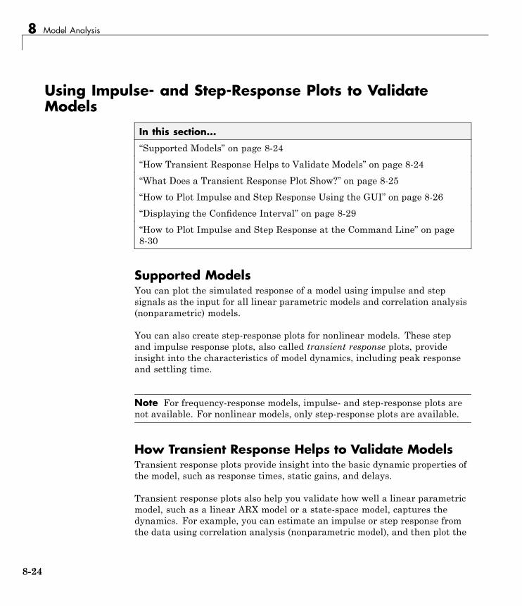
8 Model Analysis
Using Impulse- and Step-Response Plots to ValidateModels
In this section...
“Supported Models” on page 8-24“How Transient Response Helps to Validate Models” on page 8-24“What Does a Transient Response Plot Show?” on page 8-25“How to Plot Impulse and Step Response Using the GUI” on page 8-26“Displaying the Confidence Interval” on page 8-29“How to Plot Impulse and Step Response at the Command Line” on page8-30
Supported ModelsYou can plot the simulated response of a model using impulse and stepsignals as the input for all linear parametric models and correlation analysis(nonparametric) models.
You can also create step-response plots for nonlinear models. These stepand impulse response plots, also called transient response plots, provideinsight into the characteristics of model dynamics, including peak responseand settling time.
Note For frequency-response models, impulse- and step-response plots arenot available. For nonlinear models, only step-response plots are available.
How Transient Response Helps to Validate ModelsTransient response plots provide insight into the basic dynamic properties ofthe model, such as response times, static gains, and delays.
Transient response plots also help you validate how well a linear parametricmodel, such as a linear ARX model or a state-space model, captures thedynamics. For example, you can estimate an impulse or step response fromthe data using correlation analysis (nonparametric model), and then plot the
8-24

Using Impulse- and Step-Response Plots to Validate Models
correlation analysis result on top of the transient responses of the parametricmodels.
Because nonparametric and parametric models are derived using differentalgorithms, agreement between these models increases confidence in theparametric model results.
What Does a Transient Response Plot Show?Transient response plots show the value of the impulse or step response onthe vertical axis. The horizontal axis is in units of time you specified for thedata used to estimate the model.
The impulse response of a dynamic model is the output signal that resultswhen the input is an impulse. That is, u(t) is zero for all values of t except att=0, where u(0)=1. In the following difference equation, you can compute theimpulse response by setting y(-T)=y(-2T)=0, u(0)=1, and u(t>0)=0.
y t y t T y t Tu t u t T
( ) . ( ) . ( ). ( ) . ( )
− − + − =+ −
1 5 0 7 20 9 0 5
The step response is the output signal that results from a step input, whereu(t<0)=0 and u(t>0)=1.
If your model includes a noise model, you can display the transient responseof the noise model associated with each output channel. For more informationabout how to display the transient response of the noise model, see “How toPlot Impulse and Step Response Using the GUI” on page 8-26.
The following figure shows a sample Transient Response plot, created inthe System Identification Tool GUI.
8-25

8 Model Analysis
How to Plot Impulse and Step Response Using theGUITo create a transient analysis plot in the System Identification Tool GUI,select the Transient resp check box in theModel Views area. For generalinformation about creating and working with plots, see “Working with Plotsin the System Identification Tool GUI” on page 12-15.
To include or exclude a model on the plot, click the corresponding model iconin the System Identification Tool GUI. Active models display a thick lineinside the Model Board icon.
The following table summarizes the Transient Response plot settings.
Transient Response Plot Settings
Action Command
Display step response for linearor nonlinear model.
Select Options > Step response.
8-26
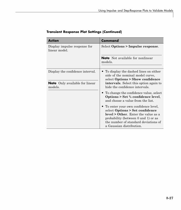
Using Impulse- and Step-Response Plots to Validate Models
Transient Response Plot Settings (Continued)
Action Command
Display impulse response forlinear model.
Select Options > Impulse response.
Note Not available for nonlinearmodels.
Display the confidence interval.
Note Only available for linearmodels.
• To display the dashed lines on eitherside of the nominal model curve,select Options > Show confidenceintervals. Select this option again tohide the confidence intervals.
• To change the confidence value, selectOptions > Set % confidence level,and choose a value from the list.
• To enter your own confidence level,select Options > Set confidencelevel > Other. Enter the value as aprobability (between 0 and 1) or asthe number of standard deviations ofa Gaussian distribution.
8-27

8 Model Analysis
Transient Response Plot Settings (Continued)
Action Command
Change time span over whichthe impulse or step response iscalculated. For a scalar timespan T, the resulting response isplotted from -T/4 to T.
Note To change the time spanof models you estimated usingcorrelation analysis models,select Estimate > Correlationmodels and reestimate themodel using a new time span.
• Select Options > Time span (timeunits), and choose a new time spanin units of time you specified for themodel.
• To enter your own time span,select Options > Time span (timeunits) > Other, and enter the totalresponse duration.
• To use the time span based on modeldynamics, type [] or default.
The default time span is computedbased on the model dynamics andmight be different for differentmodels. For nonlinear models, thedefault time span is 10.
Toggle between line plot or stemplot.
Tip Use a stem plot fordisplaying impulse response.
Select Style > Line plot orStyle > Stem plot.
8-28

Using Impulse- and Step-Response Plots to Validate Models
Transient Response Plot Settings (Continued)
Action Command
(Multiple-output system only)Select an input-output pairto view the noise spectrumcorresponding to those channels.
Select the output by name in theChannel menu.
If the plotted models include a noisemodel, you can display the transientresponse properties associated witheach output channel. The name of thechannel has the format e@OutputName,where OutputName is the name of theoutput channel corresponding to thenoise model.
(Step response for nonlinearmodels only)Set level of the input step.
Note Formultiple-inputmodels,the input-step level applies onlyto the input channel you selectedto display in the plot.
Select Options > Step Size, and thenchose from two options:
• 0–>1 sets the lower level to 0 and theupper level to 1.
• Other opens the Step Level dialogbox, where you enter the values forthe lower and upper level values.
Displaying the Confidence IntervalIn addition to the transient-response curve, you can display a confidenceinterval on the plot. To learn how to show or hide confidence interval, see thedescription of the plot settings in “How to Plot Impulse and Step ResponseUsing the GUI” on page 8-26.
The confidence interval corresponds to the range of response values with aspecific probability of being the actual response of the system. The toolboxuses the estimated uncertainty in the model parameters to calculateconfidence intervals and assumes the estimates have a Gaussian distribution.
For example, for a 95% confidence interval, the region around the nominalcurve represents the range of values that have a 95% probability of being the
8-29

8 Model Analysis
true system response. You can specify the confidence interval as a probability(between 0 and 1) or as the number of standard deviations of a Gaussiandistribution. For example, a probability of 0.99 (99%) corresponds to 2.58standard deviations.
Note The calculation of the confidence interval assumes that the modelsufficiently describes the system dynamics and the model residuals passindependence tests.
How to Plot Impulse and Step Response at theCommand LineYou can plot impulse- and step-response plots using the impulse and stepcommands, respectively.
All plot commands have the same basic syntax, as follows:
• To plot one model, use the syntax command(model).
• To plot several models, use the syntaxcommand(model1,model2,...,modelN).
In this case, command represents any of the plotting commands.
To display confidence intervals for a specified number of standard deviations,use the following syntax:
command(model,'sd',sd)
where sd is the number of standard deviations of a Gaussian distribution. Forexample, a confidence value of 99% for the nominal model curve correspondsto 2.58 standard deviations.
To display a filled confidence region, use the following syntax:
command(model,'sd',sd,'fill')
8-30
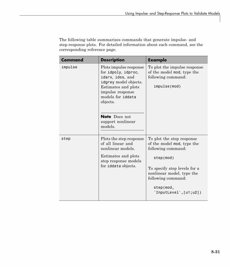
Using Impulse- and Step-Response Plots to Validate Models
The following table summarizes commands that generate impulse- andstep-response plots. For detailed information about each command, see thecorresponding reference page.
Command Description Example
impulse Plots impulse responsefor idpoly, idproc,idarx, idss, andidgrey model objects.Estimates and plotsimpulse responsemodels for iddataobjects.
Note Does notsupport nonlinearmodels.
To plot the impulse responseof the model mod, type thefollowing command:
impulse(mod)
step Plots the step responseof all linear andnonlinear models.
Estimates and plotsstep response modelsfor iddata objects.
To plot the step responseof the model mod, type thefollowing command:
step(mod)
To specify step levels for anonlinear model, type thefollowing command:
step(mod,'InputLevel',[u1;u2])
8-31

8 Model Analysis
Using Frequency-Response Plots to Validate Models
In this section...
“What Is Frequency Response?” on page 8-32“How Frequency Response Helps to Validate Models” on page 8-33“What Does a Frequency-Response Plot Show?” on page 8-34“How to Plot Bode Plots Using the GUI” on page 8-35“How to Plot Bode and Nyquist Plots at the Command Line” on page 8-38
What Is Frequency Response?Frequency response plots show the complex values of a transfer function as afunction of frequency.
In the case of linear dynamic systems, the transfer function G is essentiallyan operator that takes the input u of a linear system to the output y:
y Gu=
For a continuous-time system, the transfer function relates the Laplacetransforms of the input U(s) and output Y(s):
Y s G s U s( ) ( ) ( )=
In this case, the frequency function G(iw) is the transfer function evaluatedon the imaginary axis s=iw.
For a discrete-time system sampled with a time interval T, the transferfunction relates the Z-transforms of the input U(z) and output Y(z):
Y z G z U z( ) ( ) ( )=
In this case, the frequency function G(eiwT) is the transfer function G(z)evaluated on the unit circle. The argument of the frequency function G(eiwT)
8-32

Using Frequency-Response Plots to Validate Models
is scaled by the sampling interval T to make the frequency function periodic
with the sampling frequency 2πT .
How Frequency Response Helps to Validate ModelsYou can plot the frequency response of a model to gain insight into thecharacteristics of linear model dynamics, including the frequency of the peakresponse and stability margins. Frequency-response plots are available for alllinear parametric models and spectral analysis (nonparametric) models.
Note Frequency-response plots are not available for nonlinear models. Inaddition, Nyquist plots do not support time-series models that have no input.
The frequency response of a linear dynamic model describes how the modelreacts to sinusoidal inputs. If the input u(t) is a sinusoid of a certain frequency,then the output y(t) is also a sinusoid of the same frequency. However, themagnitude of the response is different from the magnitude of the input signal,and the phase of the response is shifted relative to the input signal.
Frequency response plots provide insight into linear systems dynamics, suchas frequency-dependent gains, resonances, and phase shifts. Frequencyresponse plots also contain information about controller requirements andachievable bandwidths. Finally, frequency response plots can also help youvalidate how well a linear parametric model, such as a linear ARX model or astate-space model, captures the dynamics.
One example of how frequency-response plots help validate other modelsis that you can estimate a frequency response from the data using spectralanalysis (nonparametric model), and then plot the spectral analysis resulton top of the frequency response of the parametric models. Becausenonparametric and parametric models are derived using different algorithms,agreement between these models increases confidence in the parametricmodel results.
8-33
8 Model Analysis
What Does a Frequency-Response Plot Show?System Identification Tool GUI supports the following types offrequency-response plots for linear parametric models, linear state-spacemodels, and nonparametric frequency-response models:
• Bode plot of the model response. A Bode plot consists of two plots. The top
plot shows the magnitude G by which the transfer function G magnifiesthe amplitude of the sinusoidal input. The bottom plot shows the phaseϕ = arg G by which the transfer function shifts the input. The input tothe system is a sinusoid, and the output is also a sinusoid with the samefrequency.
• Bode plot of the disturbance model, called noise spectrum. This plot is thesame as a Bode plot of the model response, but it shows the frequencyresponse of the noise model instead. For more information, see “CreatingNoise-Spectrum Plots” on page 8-40.
• (Only in the MATLAB Command Window)Nyquist plot. Plots the imaginary versus the real part of the transferfunction.
The following figure shows a sample Bode plot of the model dynamics, createdin the System Identification Tool GUI.
8-34

Using Frequency-Response Plots to Validate Models
How to Plot Bode Plots Using the GUITo create a frequency-response plot for parametric linear models in the SystemIdentification Tool GUI, select the Frequency resp check box in the ModelViews area. For general information about creating and working with plots,see “Working with Plots in the System Identification Tool GUI” on page 12-15.
To include or exclude a model on the plot, click the corresponding model iconin the System Identification Tool GUI. Active models display a thick lineinside the Model Board icon.
In addition to the frequency-response curve, you can display a confidenceinterval on the plot. The confidence interval corresponds to the range ofresponse values with a specific probability of being the actual response of thesystem. The toolbox uses the estimated uncertainty in the model parametersto calculate confidence intervals and assumes the estimates have a Gaussiandistribution.
For example, for a 95% confidence interval, the region around the nominalcurve represents the range of values that have a 95% probability of being the
8-35

8 Model Analysis
true system response. You can specify the confidence interval as a probability(between 0 and 1) or as the number of standard deviations of a Gaussiandistribution. For example, a probability of 0.99 (99%) corresponds to 2.58standard deviations.
The following table summarizes the Frequency Function plot settings.
Frequency Function Plot Settings
Action Command
Display the confidenceinterval.
• To display the dashed lines on eitherside of the nominal model curve, selectOptions > Show confidence intervals.Select this option again to hide theconfidence intervals.
• To change the confidence value, selectOptions > Set % confidence level, andchoose a value from the list.
• To enter your own confidence level, selectOptions > Set confidence level > Other.Enter the value as a probability (between0 and 1) or as the number of standarddeviations of a Gaussian distribution.
8-36
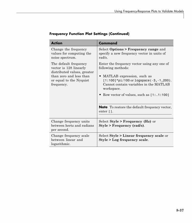
Using Frequency-Response Plots to Validate Models
Frequency Function Plot Settings (Continued)
Action Command
Change the frequencyvalues for computing thenoise spectrum.
The default frequencyvector is 128 linearlydistributed values, greaterthan zero and less thanor equal to the Nyquistfrequency.
Select Options > Frequency range andspecify a new frequency vector in units ofrad/s.
Enter the frequency vector using any one offollowing methods:
• MATLAB expression, such as[1:100]*pi/100 or logspace(-3,-1,200).Cannot contain variables in the MATLABworkspace.
• Row vector of values, such as [1:.1:100]
Note To restore the default frequency vector,enter [].
Change frequency unitsbetween hertz and radiansper second.
Select Style > Frequency (Hz) orStyle > Frequency (rad/s).
Change frequency scalebetween linear andlogarithmic.
Select Style > Linear frequency scale orStyle > Log frequency scale.
8-37

8 Model Analysis
Frequency Function Plot Settings (Continued)
Action Command
Change amplitude scalebetween linear andlogarithmic.
Select Style > Linear amplitude scale orStyle > Log amplitude scale.
(Multiple-output systemonly)Select an input-output pairto view the noise spectrumcorresponding to thosechannels.
Note You cannot viewcross spectra betweendifferent outputs.
Select the output by name in the Channelmenu.
How to Plot Bode and Nyquist Plots at the CommandLineYou can plot Bode and Nyquist plots for linear models using the bode, ffplot,and nyquist commands.
All plot commands have the same basic syntax, as follows:
• To plot one model, use the syntax command(model).
• To plot several models, use the syntaxcommand(model1,model2,...,modelN).
In this case, command represents any of the plotting commands.
To display confidence intervals for a specified number of standard deviations,use the following syntax:
command(model,'sd',sd)
8-38

Using Frequency-Response Plots to Validate Models
where sd is the number of standard deviations of a Gaussian distribution. Forexample, a confidence value of 99% for the nominal model curve correspondsto 2.58 standard deviations.
To display a filled confidence region, use the following syntax:
command(model,'sd',sd,'fill')
The following table summarizes commands that generate Bode and Nyquistplots for linear models. For detailed information about each command andhow to specify the frequency values for computing the response, see thecorresponding reference page.
Command Description Example
bode Plots the magnitudeand phase of thefrequency response ona logarithmic frequencyscale.
To create the bode plotof the model mod, usethe following command:
bode(mod)
ffplot Plots the magnitudeand phase of thefrequency responseon a linear frequencyscale (hertz).
To create the bode plotof the model mod, usethe following command:
ffplot(mod)
nyquist Plots the imaginaryversus real part of thetransfer function.
Note Does not supporttime-series models.
To plot the frequencyresponse of the modelmod, use the followingcommand:
nyquist(mod)
8-39
8 Model Analysis
Creating Noise-Spectrum Plots
In this section...
“Supported Models” on page 8-40“What Does a Noise Spectrum Plot Show?” on page 8-40“Displaying the Confidence Interval” on page 8-41“How to Plot the Noise Spectrum Using the GUI” on page 8-42“How to Plot the Noise Spectrum at the Command Line” on page 8-45
Supported ModelsWhen you estimate the noise model of your linear system, you can plot thespectrum of the estimated noise model. Noise-spectrum plots are available forall linear parametric models and spectral analysis (nonparametric) models.
Note For nonlinear models and correlation analysis models, noise-spectrumplots are not available. For time-series models, you can only generatenoise-spectrum plots for parametric and spectral-analysis models.
What Does a Noise Spectrum Plot Show?The general equation of a linear dynamic system is given by:
y t G z u t v t( ) ( ) ( ) ( )= +
In this equation, G is an operator that takes the input to the output andcaptures the system dynamics, and v is the additive noise term. The toolboxtreats the noise term as filtered white noise, as follows:
v t H z e t( ) ( ) ( )=
The toolbox computes both H and λ during the estimation of the noise modeland stores these quantities as model properties. The H(z) operator representsthe noise model. e(t) is a white-noise source with variance λ .
8-40

Creating Noise-Spectrum Plots
Whereas the frequency-response plot shows the response of G, thenoise-spectrum plot shows the frequency-response of the noise model H.
For input-output models, the noise spectrum is given by the followingequation:
ΦviH e( )ω λ ω= ( ) 2
For time-series models (no input), the vertical axis of the noise-spectrum plotis the same as the dynamic model spectrum. These axes are the same becausethere is no input for time series and y He= .
Note You can avoid estimating the noise model by selecting the Output-Errormodel structure or by setting the DisturbanceModel property value to 'None'for a state space model. If you choose to not estimate a noise model foryour system, then H and the noise spectrum amplitude are equal to 1 at allfrequencies.
Displaying the Confidence IntervalIn addition to the noise-spectrum curve, you can display a confidence intervalon the plot. To learn how to show or hide confidence interval, see thedescription of the plot settings in “How to Plot the Noise Spectrum Usingthe GUI” on page 8-42.
The confidence interval corresponds to the range of power-spectrum valueswith a specific probability of being the actual noise spectrum of the system.The toolbox uses the estimated uncertainty in the model parameters tocalculate confidence intervals and assumes the estimates have a Gaussiandistribution.
For example, for a 95% confidence interval, the region around the nominalcurve represents the range of values that have a 95% probability of being thetrue system noise spectrum. You can specify the confidence interval as aprobability (between 0 and 1) or as the number of standard deviations of a
8-41
8 Model Analysis
Gaussian distribution. For example, a probability of 0.99 (99%) correspondsto 2.58 standard deviations.
Note The calculation of the confidence interval assumes that the modelsufficiently describes the system dynamics and the model residuals passindependence tests.
How to Plot the Noise Spectrum Using the GUITo create a noise spectrum plot for parametric linear models in the GUI,select the Noise spectrum check box in theModel Views area. For generalinformation about creating and working with plots, see “Working with Plotsin the System Identification Tool GUI” on page 12-15.
To include or exclude a model on the plot, click the corresponding model iconin the System Identification Tool GUI. Active models display a thick lineinside the Model Board icon.
The following figure shows a sample Noise Spectrum plot.
8-42
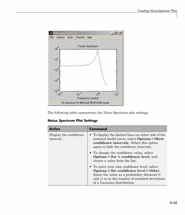
Creating Noise-Spectrum Plots
The following table summarizes the Noise Spectrum plot settings.
Noise Spectrum Plot Settings
Action Command
Display the confidenceinterval.
• To display the dashed lines on either side of thenominal model curve, select Options > Showconfidence intervals. Select this optionagain to hide the confidence intervals.
• To change the confidence value, selectOptions > Set % confidence level, andchoose a value from the list.
• To enter your own confidence level, selectOptions > Set confidence level > Other.Enter the value as a probability (between 0and 1) or as the number of standard deviationsof a Gaussian distribution.
8-43

8 Model Analysis
Noise Spectrum Plot Settings (Continued)
Action Command
Change the frequencyvalues for computingthe noise spectrum.
The default frequencyvector is 128 linearlydistributed values,greater than zero andless than or equal to theNyquist frequency.
Select Options > Frequency range and specifya new frequency vector in units of radians persecond.
Enter the frequency vector using any one offollowing methods:
• MATLAB expression, such as [1:100]*pi/100or logspace(-3,-1,200). Cannot containvariables in the MATLAB workspace.
• Row vector of values, such as [1:.1:100]
Tip To restore the default frequency vector, enter[].
Change frequency unitsbetween hertz andradians per second.
Select Style > Frequency (Hz) orStyle > Frequency (rad/s).
Change frequency scalebetween linear andlogarithmic.
Select Style > Linear frequency scale orStyle > Log frequency scale.
8-44

Creating Noise-Spectrum Plots
Noise Spectrum Plot Settings (Continued)
Action Command
Change amplitude scalebetween linear andlogarithmic.
Select Style > Linear amplitude scale orStyle > Log amplitude scale.
(Multiple-outputsystem only)Select an input-outputpair to view the noisespectrum correspondingto those channels.
Note You cannot viewcross spectra betweendifferent outputs.
Select the output by name in the Channel menu.
How to Plot the Noise Spectrum at the Command LineYou can plot the frequency-response of the noise model.
First, select the portion of the model object that corresponds to the noisemodel H. For example, to select the noise model in the model object m, typethe following command:
m_noise=m('noise')
Tip You can abbreviate the command to m_noise=m('n').
To plot the frequency-response of the noise model, use the bode command:
bode(m_noise)
To determine if your estimated noise model is good enough, you can comparethe frequency-response of the estimated noise-model H to the estimated
8-45

8 Model Analysis
frequency response of v(t). To compute v(t), which represents the actual noiseterm in the system, use the following commands:
ysimulated = sim(m,data);v = ymeasured-ysimulated;
ymeasured is data.y. v is the noise term v(t), as described in “What Does aNoise Spectrum Plot Show?” on page 8-40 and corresponds to the differencebetween the simulated response ysimulated and the actual responseymeasured.
To compute the frequency-response model of the actual noise, use spa:
V = spa(v);
The toolbox uses the following equation to compute the noise spectrum ofthe actual noise:
Φv viR e( )ω τ
τ
ωτ= ( )=−∞
∞−∑
The covariance function Rv is given in terms of E, which denotes themathematical expectation, as follows:
R Ev t v tv τ τ( ) = ( ) −( )
To compare the parametric noise-model H to the (nonparametric)frequency-response estimate of the actual noise v(t), use bode:
bode(V,m('noise'))
If the parametric and the nonparametric estimates of the noise spectra aredifferent, then you might need a higher-order noise model.
8-46

Using Pole-Zero Plots to Validate Models
Using Pole-Zero Plots to Validate Models
In this section...
“Supported Models” on page 8-47“What Does a Pole-Zero Plot Show?” on page 8-47“How to Plot Model Poles and Zeros Using the GUI” on page 8-48“How to Plot Poles and Zeros at the Command Line” on page 8-50“Reducing Model Order Using Pole-Zero Plots” on page 8-51
Supported ModelsYou can create pole-zero plots of linear input-output polynomial, state-space,and grey-box models.
What Does a Pole-Zero Plot Show?The general equation of a linear dynamic system is given by:
y t G z u t v t( ) ( ) ( ) ( )= +
In this equation, G is an operator that takes the input to the output andcaptures the system dynamics, and v is the additive noise term.
The poles of a linear system are the roots of the denominator of the transferfunction G. The poles have a direct influence on the dynamic properties ofthe system. The zeros are the roots of the numerator of G. If you estimateda noise model H in addition to the dynamic model G, you can also view thepoles and zeros of the noise model.
Zeros and the poles are equivalent ways of describing the coefficients of alinear difference equation, such as the ARX model. Poles are associated withthe output side of the difference equation, and zeros are associated with theinput side of the equation. The number of poles is equal to the number ofsampling intervals between the most-delayed and least-delayed output. Thenumber of zeros) is equal to the number of sampling intervals between the
8-47

8 Model Analysis
most-delayed and least-delayed input. For example, there two poles and onezero in the following ARX model:
y t y t T y t Tu t u t T
( ) . ( ) . ( ). ( ) . ( )
− − + − =+ −
1 5 0 7 20 9 0 5
The following figure shows a sample pole-zero plot of the model withconfidence intervals. x indicate poles and o indicate zeros.
How to Plot Model Poles and Zeros Using the GUITo create a pole-zero plot for parametric linear models in the SystemIdentification Tool GUI, select the Zeros and poles check box in the ModelViews area. For general information about creating and working with plots,see “Working with Plots in the System Identification Tool GUI” on page 12-15.
To include or exclude a model on the plot, click the corresponding model iconin the System Identification Tool GUI. Active models display a thick lineinside the Model Board icon.
8-48

Using Pole-Zero Plots to Validate Models
In addition, you can display a confidence interval for each pole and zero on theplot. The confidence interval corresponds to the range of pole or zero valueswith a specific probability of being the actual pole or zero of the system. Thetoolbox uses the estimated uncertainty in the model parameters to calculateconfidence intervals and assumes the estimates have a Gaussian distribution.
For example, for a 95% confidence interval, the region around the nominalpole or zero value represents the range of values that have a 95% probabilityof being the true system pole or zero value. You can specify the confidenceinterval as a probability (between 0 and 1) or as the number of standarddeviations of a Gaussian distribution. For example, a probability of 0.99 (99%)corresponds to 2.58 standard deviations.
The following table summarizes the Zeros and Poles plot settings.
Zeros and Poles Plot Settings
Action Command
Display the confidenceinterval.
• To display the dashed lines on either sideof the nominal pole and zero values, selectOptions > Show confidence intervals.Select this option again to hide the confidenceintervals.
• To change the confidence value, selectOptions > Set % confidence level, andchoose a value from the list.
• To enter your own confidence level, selectOptions > Set confidence level > Other.Enter the value as a probability (between 0and 1) or as the number of standard deviationsof a Gaussian distribution.
Show real andimaginary axes.
Select Style > Re/Im-axes. Select this optionagain to hide the axes.
8-49

8 Model Analysis
Zeros and Poles Plot Settings (Continued)
Action Command
Show the unit circle. Select Style > Unit circle. Select this optionagain to hide the unit circle.
(Multiple-output systemonly)Select an input-outputpair to view the polesand zeros correspondingto those channels.
Select the output by name in the Channelmenu.
How to Plot Poles and Zeros at the Command LineYou can create a pole-zero plot for linear polynomial, linear state-space, andlinear grey-box models using the pzmap command. pzmap lets you includeseveral models on a plot.
To display confidence intervals for a specified number of standard deviations,use the following syntax:
pzmap(model,'sd',sd)
where sd is the number of standard deviations of a Gaussian distribution. Forexample, a confidence value of 99% for the nominal model curve correspondsto 2.58 standard deviations.
Command Description Example
pzmap Plots zeros and polesof the model on theS-plane or Z-plane forcontinuous-time ordiscrete-time model,respectively.
To plot the poles andzeros of the modelmod, use the followingcommand:
pzmap(mod)
For detailed information about pzmap, see the corresponding reference page.
8-50
Using Pole-Zero Plots to Validate Models
Reducing Model Order Using Pole-Zero PlotsYou can use pole-zero plots to evaluate whether it might be useful to reducemodel order. When confidence intervals for a pole-zero pair overlap, thisoverlap indicates a possible pole-zero cancelation.
For example, you can use the following syntax to plot a 1-standard-deviationconfidence interval around model poles and zeros.
pzmap(model,'sd',1)
If poles and zeros overlap, try estimating a lower order model.
Always validate model output and residuals to see if the quality of thefit changes after reducing model order. If the plot indicates pole-zerocancellations, but reducing model order degrades the fit, then the extrapoles probably describe noise. In this case, you can choose a different modelstructure that decouples system dynamics and noise. For example, tryARMAX, Output-Error, or Box-Jenkins polynomial model structures withan A or F polynomial of an order equal to that of the number of uncanceledpoles. For more information about estimating linear polynomial models, see“Identifying Input-Output Polynomial Models” on page 3-41.
8-51

8 Model Analysis
Using Nonlinear ARX Plots to Validate Models
In this section...
“About Nonlinear ARX Plots” on page 8-52“How to Plot Nonlinear ARX Plots Using the GUI” on page 8-52“Configuring the Nonlinear ARX Plot” on page 8-53“Axis Limits, Legend, and 3-D Rotation” on page 8-54“How to Plot Nonlinear ARX Plots at the Command Line” on page 8-55
About Nonlinear ARX PlotsThe Nonlinear ARX plot displays the characteristics of model nonlinearitiesas a function of one or two regressors. For more information about estimatingnonlinear ARX models, see “Identifying Nonlinear ARX Models” on page 4-4.
Examining a nonlinear ARX plot can help you gain insight into whichregressors have the strongest effect on the model output. Understanding therelative importance of the regressors on the output can help you decide whichregressors should be included in the nonlinear function.
Furthermore, you can create several nonlinear models for the same dataset using different nonlinearity estimators, such a wavelet network andtree partition, and then compare the nonlinear surfaces of these models.Agreement between nonlinear surfaces increases the confidence that thesenonlinear models capture the true dynamics of the system.
How to Plot Nonlinear ARX Plots Using the GUITo create a nonlinear ARX plot in the System Identification Tool GUI, selectthe Nonlinear ARX check box in the Model Views area. For generalinformation about creating and working with plots, see “Working with Plotsin the System Identification Tool GUI” on page 12-15.
Note The Nonlinear ARX check box is unavailable if you do not have anonlinear ARX model in the Model Board.
8-52
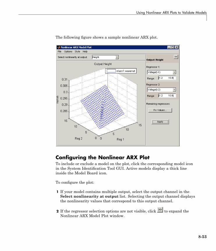
Using Nonlinear ARX Plots to Validate Models
The following figure shows a sample nonlinear ARX plot.
Configuring the Nonlinear ARX PlotTo include or exclude a model on the plot, click the corresponding model iconin the System Identification Tool GUI. Active models display a thick lineinside the Model Board icon.
To configure the plot:
1 If your model contains multiple output, select the output channel in theSelect nonlinearity at output list. Selecting the output channel displaysthe nonlinearity values that correspond to this output channel.
2 If the regressor selection options are not visible, click to expand theNonlinear ARX Model Plot window.
8-53
8 Model Analysis
3 Select Regressor 1 from the list of available regressors. In the Rangefield, enter the range of values to include on the plot for this regressor. Theregressor values are plotted on the Reg1 axis.
4 Specify a second regressor for a 3-D plot by selecting one of the followingtypes of options:
• Select Regressor 2 to display three axes. In the Range field, enter therange of values to include on the plot for this regressor. The regressorvalues are plotted on the Reg2 axis.
• Select <none> in the Regressor 2 list to display only two axes.
5 To fix the values of the regressor that are not displayed, click Fix Values.In the Fix Regressor Values dialog box, double-click the Value cell to editthe constant value of the corresponding regressor. The default values aredetermined during model estimation. Click OK.
6 In the Nonlinear ARX Model Plot window, click Apply to update the plot.
7 To change the grid of the regressor space along each axis, Options > Setnumber of samples, and enter the number of samples to use for eachregressor. Click Apply and then Close.
For example, if the number of samples is 20, each regressor variablecontains 20 points in its specified range. For a 3-D plots, this results inevaluating the nonlinearity at 20 x 20 = 400 points.
Axis Limits, Legend, and 3-D RotationThe following table summarizes the commands to modify the appearanceof the Nonlinear ARX plot.
Changing Appearance of the Nonlinear ARX Plot
Action Command
Change axis limits. Select Options > Set axis limits toopen the Axis Limits dialog box, andedit the limits. Click Apply.
8-54

Using Nonlinear ARX Plots to Validate Models
Changing Appearance of the Nonlinear ARX Plot (Continued)
Action Command
Hide or show the legend. Select Style > Legend. Select thisoption again to show the legend.
(Three axes only)Rotate in three dimensions.
Note Available only when youhave selected two regressors asindependent variables.
Select Style > 3D Rotate anddrag the axes on the plot toa new orientation. To disablethree-dimensional rotation, selectStyle > 3D Rotate again.
How to Plot Nonlinear ARX Plots at the CommandLineYou can plot the nonlinearity shape of nonlinear ARX models using thefollowing syntax:
plot(model)
model must be an idnlarx model object. You can use additional plotarguments to specify the following information:
• Include multiple nonlinear ARX models on the plot.
• Configure the regressor values for computing the nonlinearity values.
The plot command opens the Nonlinear ARX Model Plot window. Formore information about working with this plot window, see “Configuringthe Nonlinear ARX Plot” on page 8-53 and “Axis Limits, Legend, and 3-DRotation” on page 8-54.
For detailed information about plot, type the following command at theprompt:
help idnlarx/plot
8-55

8 Model Analysis
Using Hammerstein-Wiener Plots to Validate Models
In this section...
“About Hammerstein-Wiener Plots” on page 8-56“How to Create Hammerstein-Wiener Plots in the GUI” on page 8-56“How to Plot Hammerstein-Wiener Plots at the Command Line” on page8-58“Plotting Nonlinear Block Characteristics” on page 8-58“Plotting Linear Block Characteristics” on page 8-59
About Hammerstein-Wiener PlotsHammerstein-Wiener model plot lets you explore the characteristics of thelinear block and the static nonlinearities of the Hammerstein-Wiener model.For more information about estimating nonlinear Hammerstein-Wienermodels, see “Identifying Hammerstein-Wiener Models” on page 4-15.
Examining a Hammerstein-Wiener plot can help you determine whether youchose an unnecessarily complicated nonlinearity for modeling your system.For example, if you chose a piece-wise-linear nonlinearity (which is verygeneral), but the plot indicates saturation behavior, then you can estimate anew model using the simpler saturation nonlinearity instead.
For multivariable systems, you can use the Hammerstein-Wiener plotto determine whether to exclude nonlinearities for specific channels. Ifthe nonlinearity for a specific input or output channel does not exhibitstrong nonlinear behavior, you can estimate a new model after setting thenonlinearity at that channel to unit gain.
How to Create Hammerstein-Wiener Plots in the GUITo create a Hammerstein-Wiener plot in the System Identification Tool GUI,select the Hamm-Wiener check box in the Model Views area. For generalinformation about creating and working with plots, see “Working with Plotsin the System Identification Tool GUI” on page 12-15.
8-56
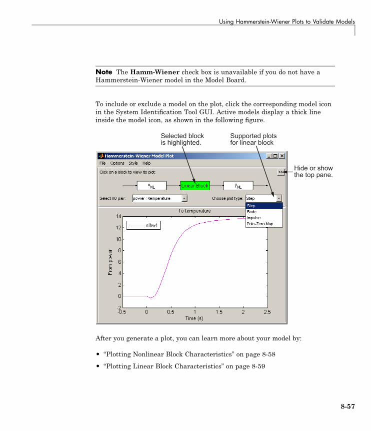
Using Hammerstein-Wiener Plots to Validate Models
Note The Hamm-Wiener check box is unavailable if you do not have aHammerstein-Wiener model in the Model Board.
To include or exclude a model on the plot, click the corresponding model iconin the System Identification Tool GUI. Active models display a thick lineinside the model icon, as shown in the following figure.
����� ����2����������&
"���� ���������� ����� ����$
"�������$�����3���3���&
After you generate a plot, you can learn more about your model by:
• “Plotting Nonlinear Block Characteristics” on page 8-58
• “Plotting Linear Block Characteristics” on page 8-59
8-57
8 Model Analysis
How to Plot Hammerstein-Wiener Plots at theCommand LineYou can plot input and output nonlinearity and linear responses forHammerstein-Wiener models using the following syntax:
plot(model)
model must be an idnlhw model object. You can use additional plotarguments to specify the following information:
• Include several Hammerstein-Wiener models on the plot.
• Configure how to evaluate the nonlinearity at each input and outputchannel.
• Specify the time or frequency values for computing transient and frequencyresponse plots of the linear block.
The plot command opens the Hammerstein-Wiener Model Plot window.For more information about working with this plot window, see “PlottingNonlinear Block Characteristics” on page 8-58 and “Plotting Linear BlockCharacteristics” on page 8-59.
For detailed information about plot, type the following command at theprompt:
help idnlhw/plot
Plotting Nonlinear Block CharacteristicsThe Hammerstein-Wiener model can contain up to two nonlinear blocks. Thenonlinearity at the input to the Linear Block is labeled uNL and is called theinput nonlinearity. The nonlinearity at the output of the Linear Block islabeled yNL and is called the output nonlinearity.
To configure the plot, perform the following steps:
1 If the top pane is not visible, click to expand the Hammerstein-WienerModel Plot window.
2 Select the nonlinear block you want to plot:
8-58

Using Hammerstein-Wiener Plots to Validate Models
• To plot uNL as a command of the input data, click the uNL block.
• To plot yNL as a command of its inputs, click the yNL block.
The selected block is highlighted in green.
Note An input to the output nonlinearity block yNL is the output from theLinear Block and not the measured input data.
3 If your model contains multiple variables, select the channel in the Selectnonlinearity at channel list. Selecting the channel updates the plotand displays the nonlinearity values versus the corresponding input tothis nonlinear block.
4 To change the range of the horizontal axis, select Options > Set inputrange to open the Range for Input to Nonlinearity dialog box. Enter therange using the format [MinValue MaxValue]. Click Apply and thenClose to update the plot.
Plotting Linear Block CharacteristicsThe Hammerstein-Wiener model contains one Linear Block that representsthe embedded linear model.
To configure the plot:
1 If the top pane is not visible, click to expand the Hammerstein-WienerModel Plot window.
2 Click the Linear Block to select it. The Linear Block is highlighted in green.
3 In the Select I/O pair list, select the input and output data pair for whichto view the response.
4 In the Choose plot type list, select the linear plot from the followingoptions:
• Step
• Impulse
8-59

8 Model Analysis
• Bode
• Pole-Zero Map
5 If you selected to plot step or impulse response, you can set the time span.Select Options > Time span and enter a new time span in units of timeyou specified for the model.
For a time span T, the resulting response is plotted from -T/4 to T. Thedefault time span is 10.
Click Apply and then Close.
6 If you selected to plot a Bode plot, you can set the frequency range.
The default frequency vector is 128 linearly distributed values, greaterthan zero and less than or equal to the Nyquist frequency. To change therange, select Options > Frequency range, and specify a new frequencyvector in units of rad per model time units.
Enter the frequency vector using any one of following methods:
• MATLAB expression, such as [1:100]*pi/100 or logspace(-3,-1,200).Cannot contain variables in the MATLAB workspace.
• Row vector of values, such as [1:.1:100].
Click Apply and then Close.
8-60

Using Akaike’s Criteria to Validate Models
Using Akaike’s Criteria to Validate Models
In this section...
“Definition of FPE” on page 8-61“Computing FPE” on page 8-62“Definition of AIC” on page 8-62“Computing AIC” on page 8-63
Definition of FPEAkaike’s Final Prediction Error (FPE) criterion provides a measure of modelquality by simulating the situation where the model is tested on a differentdata set. After computing several different models, you can compare themusing this criterion. According to Akaike’s theory, the most accurate modelhas the smallest FPE.
Note If you use the same data set for both model estimation and validation,the fit always improves as you increase the model order and, therefore, theflexibility of the model structure.
Akaike’s Final Prediction Error (FPE) is defined by the following equation:
FPE Vd
Nd
N=
+−
⎛
⎝⎜⎜
⎞
⎠⎟⎟
1
1
where V is the loss function, d is the number of estimated parameters, and Nis the number of values in the estimation data set.
The toolbox assumes that the final prediction error is asymptotic for d<<Nand uses the following approximation to compute FPE:
FPE V dN= +( )1 2
The loss function V is defined by the following equation:
8-61
8 Model Analysis
V t tN N NTN
= ( ) ( )( )⎛
⎝⎜⎜
⎞
⎠⎟⎟∑det , ,1
1ε θ ε θ
where θN represents the estimated parameters.
Computing FPEYou can compute Akaike’s Final Prediction Error (FPE) criterion for linearand nonlinear models.
Note FPE for nonlinear ARX models that include a tree partitionnonlinearity is not supported.
To compute FPE, use the fpe command, as follows:
FPE = fpe(m1,m2,m3,...,mN)
According to Akaike’s theory, the most accurate model has the smallest FPE.
You can also access the FPE value of an estimated model by accessing theFPE field of the EstimationInfo property of this model. For example, if youestimated the model m, you can access its FPE using the following command:
m.EstimationInfo.FPE
Definition of AICAkaike’s Information Criterion (AIC) provides a measure of model qualityby simulating the situation where the model is tested on a different dataset. After computing several different models, you can compare them usingthis criterion. According to Akaike’s theory, the most accurate model hasthe smallest AIC.
Note If you use the same data set for both model estimation and validation,the fit always improves as you increase the model order and, therefore, theflexibility of the model structure.
8-62
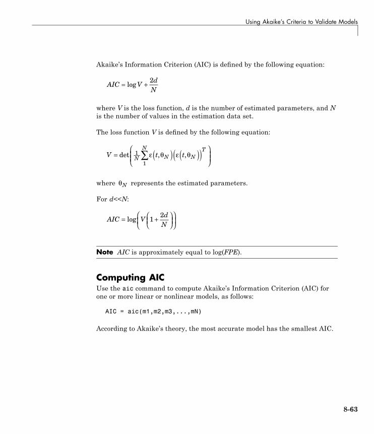
Using Akaike’s Criteria to Validate Models
Akaike’s Information Criterion (AIC) is defined by the following equation:
AIC Vd
N= +log
2
where V is the loss function, d is the number of estimated parameters, and Nis the number of values in the estimation data set.
The loss function V is defined by the following equation:
V t tN N NTN
= ( ) ( )( )⎛
⎝⎜⎜
⎞
⎠⎟⎟∑det , ,1
1ε θ ε θ
where θN represents the estimated parameters.
For d<<N:
AIC Vd
N= +⎛
⎝⎜⎞⎠⎟
⎛⎝⎜
⎞⎠⎟log 1
2
Note AIC is approximately equal to log(FPE).
Computing AICUse the aic command to compute Akaike’s Information Criterion (AIC) forone or more linear or nonlinear models, as follows:
AIC = aic(m1,m2,m3,...,mN)
According to Akaike’s theory, the most accurate model has the smallest AIC.
8-63

8 Model Analysis
Computing Model Uncertainty
In this section...
“Why Analyze Model Uncertainty?” on page 8-64“What Is Model Covariance?” on page 8-64“Viewing Model Uncertainty Information” on page 8-65
Why Analyze Model Uncertainty?In addition to estimating model parameters, the toolbox algorithms alsoestimate variability of the model parameters that result from randomdisturbances in the output.
Understanding model variability helps you to understand how different yourmodel parameters would be if you repeated the estimation using a differentdata set (with the same input sequence as the original data set) and the samemodel structure.
When validating your parametric models, check the uncertainty values.Large uncertainties in the parameters might be caused by high model orders,inadequate excitation, and poor signal-to-noise ratio in the data.
Note You can get model uncertainty data for linear parametric black-boxmodels, and both linear and nonlinear grey-box models. Supported modelobjects include idproc, idpoly, idss, idarx, idgrey, idfrd, and idnlgrey.
What Is Model Covariance?Uncertainty in the model is called model covariance.
If you estimate model uncertainty data, this information is stored in theModel.CovarianceMatrix model property. The covariance matrix is used tocompute all uncertainties in model output, Bode plots, residual plots, andpole-zero plots.
8-64
Computing Model Uncertainty
Computing the covariance matrix is based on the assumption that the modelstructure gives the correct description of the system dynamics. For modelsthat include a disturbance model H, a correct uncertainty estimate assumesthat the model produces white residuals. To determine whether you can trustthe estimated model uncertainty values, perform residual analysis testson your model, as described in “Using Residual Analysis Plots to ValidateModels” on page 8-16. If your model passes residual analysis tests, there is agood chance that the true system lies within the confidence interval and anyparameter uncertainties results from random disturbances in the output.
In the case of output-error models, where the noise model H is fixed to 1,computing the covariance matrix does not assume that the residuals arewhite. Instead, the covariance is estimated based on the estimated color of theresidual correlations. This estimation of the noise color is also performed forstate-space models with K=0, which is equivalent to an output-error model.
Viewing Model Uncertainty InformationYou can view the following uncertainty information from linear and nonlineargrey-box models:
• Uncertainties of estimated parameters.
Type present(model) at the prompt, where model represents the name ofa linear or nonlinear model.
• Confidence intervals on the linear model plots, including step-response,impulse-response, Bode, and pole-zero plots.
Confidence intervals are computed based on the variability in the modelparameters. For information about displaying confidence intervals, see thecorresponding plot section.
• Covariance matrix of the estimated parameters in linear and nonlineargrey-box models.
Type model.CovarianceMatrix at the prompt, where model represents thename of the model object.
• Estimated standard deviations of polynomial coefficients or state-spacematrices
8-65
8 Model Analysis
Type model.dA at the prompt to access the estimated standard deviationsof the model.A estimated property, where model represents the nameof the model object, and A represents any estimated model property. Ingeneral, you prefix the name of the estimated property with a d to get thestandard deviation estimate for that property. For example, to get thestandard deviation value of the A polynomial in an estimated ARX model,type model.da.
Note State-space models, estimated with free parameterization, donot have well-defined standard deviations of the matrix elements. Todisplay matrix parameter uncertainties in this case, first transform themodel to a canonical parameterization by setting the ss model propertyto model.ss = 'canon'. For more information about free and canonicalparameterizations, see “Identifying State-Space Models” on page 3-73.
• Simulated output values for linear models with standard deviations usingthe sim command.
Call the sim command with output arguments, where the second outputargument is the estimated standard deviation of each output value.For example, type [ysim,ysimsd]=sim(model,data), where ysim isthe simulated output, ysimsd contains the standard deviations on thesimulated output, and data is the simulation data.
8-66
Troubleshooting Models
Troubleshooting Models
In this section...
“About Troubleshooting Models” on page 8-67“Model Order Is Too High or Too Low” on page 8-67“Nonlinearity Estimator Produces a Poor Fit” on page 8-68“Substantial Noise in the System” on page 8-69“Unstable Models” on page 8-69“Missing Input Variables” on page 8-70“Complicated Nonlinearities” on page 8-71
About Troubleshooting ModelsDuring validation, you might find that your model output fits the validationdata poorly. You might also find some unexpected or undesirable modelcharacteristics.
If the tips suggested in these sections do not help improve your models, thena good model might not be possible for this data. For example, your datamight have poor signal-to-noise ratio, large and nonstationary disturbances,or varying system properties.
Model Order Is Too High or Too LowWhen the Model Output plot does not show a good fit, there is a good chancethat you need to try a different model order. System identification is largelya trial-and-error process when selecting model structure and model order.Ideally, you want the lowest-order model that adequately captures the systemdynamics.
You can estimate the model order as described in “Preliminary Step –Estimating Model Orders and Input Delays” on page 3-49. Typically, you usethe suggested order as a starting point to estimate the lowest possible orderwith different model structures. After each estimation, you monitor the ModelOutput and the Residual Analysis plots, and then adjust your settings forthe next estimation.
8-67
8 Model Analysis
When a low-order model fits the validation data poorly, try estimating ahigher-order model to see if the fit improves. For example, if a Model Outputplot shows that a fourth-order model gives poor results, try estimating aneighth-order model. When a higher-order model improves the fit, you canconclude that higher-order models might be required and linear models mightbe sufficient.
You should use an independent data set to validate your models. If youuse the same data set to both estimate and validate a model, the fit alwaysimproves as you increase model order, and you risk overfitting. However, ifyou use an independent data set to validate your models, the fit eventuallydeteriorates if your model orders are too high.
High-order models are more expensive to compute and result in greaterparameter uncertainty.
Nonlinearity Estimator Produces a Poor FitIn the case of nonlinear ARX and Hammerstein-Wiener models, the ModelOutput plot does not show a good fit when the nonlinearity estimator hasincorrect complexity.
You specify the complexity of piece-wise-linear, wavelet, sigmoid, andcustom networks using the number of units (NumberOfUnits nonlinearestimator property). A high number of units indicates a complex nonlinearityestimator. In the case of neural networks, you specify the complexity usingthe parameters of the network object. For more information, see the NeuralNetwork Toolbox documentation.
To select the appropriate complexity of the nonlinearity estimator, startwith a low complexity and validate the model output. Next, increate thecomplexity and validate the model output again. The model fit degrades whenthe nonlinearity estimator becomes too complex.
Note To see the model fit degrade when the nonlinearity estimator becomestoo complex, you must use an independent data set to validate the data that isdifferent from the estimation data set.
8-68

Troubleshooting Models
Substantial Noise in the SystemThere are a couple of indications that you might have substantial noise inyour system and might need to use linear model structures that are betterequipped to model noise.
One indication of noise is when a state-space model is better than an ARXmodel at reproducing the measured output; whereas the state-space structurehas sufficient flexibility to model noise, the ARX model structure is less ableto model noise because the A polynomial must account for both the systemdynamics and the noise. The following equation represents the ARX modeland shows that A couples the dynamics and the noise by appearing in thedenominator of both the dynamics term and the noise terms:
yBA
uA
e= + 1
Another indication that a noise model is needed appears in residual analysisplots when you see significant autocorrelation of residuals at nonzero lags.For more information about residual analysis, see “Using Residual AnalysisPlots to Validate Models” on page 8-16.
To model noise more carefully, use the ARMAX or the Box-Jenkins modelstructure, where the dynamics term and the noise term are modeled bydifferent polynomials.
Unstable ModelsOne of the most conclusive approaches to determining whether a linear modelis unstable is by examining the pole-zero plot of the model, which is describedin “Using Pole-Zero Plots to Validate Models” on page 8-47. The stabilitythreshold for pole values differs for discrete-time and continuous-time models,as follows:
• For stable continuous-time models, the real part of the pole is less than 0.
• For stable discrete-time models, the magnitude of the pole is less than 1.
In some cases, an unstable model is still a useful model. For example, yoursystem might be unstable without a controller, and you plan to use your
8-69

8 Model Analysis
model for control design. In this case, you can import your unstable modelinto Simulink or Control System Toolbox products.
One way to check if a nonlinear model is unstable is to plot the simulatedmodel output on top of the validation data. If the simulated output divergesfrom measured output, the model is unstable. However, agreement betweenmodel output and measured output does not guarantee stability.
In the case of linear models, if you believe that your system is stable, but yourmodel is unstable, then you can estimate the model again with a Focus settingthat guarantees stability. For example, set Focus to Stability to find the beststable model. This setting might result in a reduced model quality. For moreinformation about Focus, see the Algorithm Properties reference page.
A more advanced approach to achieving a stable model is by setting thestability threshold property to allow a margin of error. The threshold modelproperty is accessed as a field in the algorithm structure:
• For continuous-time models, set the value ofmodel.algorithm.advanced.sstability. The model is considered stableif the pole on the far right is to the left of sstability threshold.
• For discrete-time models, set the value ofmodel.algorithm.advanced.zstability. The model is considered stableif all poles inside the circle centered at the origin and with a radiuszstability.
For more information about Threshold fields for linear models, see theAlgorithm Properties reference page.
Missing Input VariablesIf the Model Output plot and Residual Analysis plot shows a poor fit andyou have already tried different structures and orders and modeled noise, itmight be that there are one or more missing inputs that have a significanteffect on the output.
Try including other measured signals in your input data, and then estimatingthe models again.
8-70

Troubleshooting Models
Inputs need not be control signals. Any measurable signal can be consideredan input, including measurable disturbances.
Complicated NonlinearitiesIf the Model Output plot and Residual Analysis plot shows a poor fit, considerif nonlinear effects are present in the system.
You can model the nonlinearities by performing a simple transformationon the signals to make the problem linear in the new variables. Forexample, if electrical power is the driving stimulus in a heating process andtemperature is the output, you can form a simple product of voltage andcurrent measurements.
If your problem is sufficiently complex and you do not have physical insightinto the problem, you might try fitting nonlinear black-box models. For moreinformation, see Chapter 4, “Nonlinear Black-Box Model Identification”.
8-71
8 Model Analysis
Next Steps After Getting an Accurate ModelAfter you get an accurate model, you can simulate or predict model output.For more information, see Chapter 9, “Simulation and Prediction”.
For linear parametric models (idmodel objects), you can perform the followingoperations:
• Transform between continuous-time and discrete-time representation.
See “Transforming Between Discrete-Time and Continuous-TimeRepresentations” on page 3-112.
• Transform between linear model representations, such as betweenpolynomial, state-space, and zero-pole representations.
See “Transforming Between Linear Model Representations” on page 3-117.
• Extract numerical data from transfer functions, pole-zero models, andstate-space matrices.
See “Extracting Parameter Values from Linear Models” on page 3-108.
For nonlinear black-box models (idnlarx and idnlhwobjects), you can performthe following operations:
• Compute a linear approximation of the nonlinear model.
See “Computing Linear Approximations of Nonlinear Black-Box Models”on page 4-33.
• Extract model parameters.
See “Extracting Parameter Values from Nonlinear Black-Box Models” onpage 4-30.
System Identification Toolbox models in the MATLAB workspace areimmediately available to other MathWorks™ products. However, if you usedthe System Identification Tool GUI to estimate models, you must first exportthe models to the MATLAB workspace.
8-72

Next Steps After Getting an Accurate Model
Tip To export a model from the GUI, drag the model icon to the ToWorkspace rectangle. For more information about working with the GUI,see Chapter 12, “Using the System Identification Tool GUI”.
If you have the Control System Toolbox software installed, you can importyour linear plant model for control-system design. For more information, see“Using Models with Control System Toolbox Software” on page 10-2.
Finally, if you have Simulink software installed, you can exchange databetween the System Identification Toolbox software and the Simulinkenvironment. For more information, see Chapter 11, “Using SystemIdentification Toolbox Blocks”.
8-73

8 Model Analysis
8-74
9
Simulation and Prediction
• “Simulating Versus Predicting Output” on page 9-2
• “Simulation and Prediction in the GUI” on page 9-4
• “Example – Simulating Model Output with Noise at the Command Line”on page 9-5
• “Example – Simulating a Continuous-Time State-Space Model at theCommand Line” on page 9-6
• “Predicting Model Output at the Command Line” on page 9-7
• “Specifying Initial States” on page 9-8
9 Simulation and Prediction
Simulating Versus Predicting OutputSimulating a model means that you compute the response of a model toa particular input. Then, the toolbox feeds this computed output into thedifferential (continuous-time) or difference (discrete-time) equation forcalculating the next output value. In this way, the simulation progressesusing previously calculated outputs in the difference equation to producethe next output; with an infinite prediction horizon (k=∞), the simulationhas no limit on how far out in time it computes output values. Simulatingmodels uses the input-data values from the validation data set to computethe output values.
Simulating models uses only past input values to compute the output values.If the model-output expression includes past outputs, the toolbox computesthe first output value using the initial conditions and the inputs. Then, thetoolbox feeds this computed output into the difference equation or differentialequation for calculating the next output value. Thus, no past outputs are usedin the computation of output at the current time.
Simulation always uses a discrete model and continuous-time models arediscretized for simulation purposes. Simulation does not involve the noisemodel unless you explicitly specify to compute the response to the noise sourceinput. During simulation, the toolbox computes the first output value usingthe initial conditions and the inputs.
Predicting future outputs of a model from previous data over a time horizon ofk samples or kTs time units—where Ts is the sampling interval and k is theprediction horizon—requires both past inputs and past outputs.
During prediction, the algorithm uses both the measured and the calculatedoutput data values in the difference equation for computing the next output.The predicted value y(t) is computed from all available inputs u(s), where
s t≤ , and all available outputs y(s), where s t k≤ −( ) . The argument srepresents the data sample number.
To make sure that the model picks up important dynamic properties, let thepredicted time horizon kT be larger than the system time constants, whereT is the sampling interval.
9-2

Simulating Versus Predicting Output
Note Prediction with k=∞ means that no previous inputs are used in thecomputation and prediction matches simulation.
9-3
9 Simulation and Prediction
Simulation and Prediction in the GUITo learn how to display simulated or predicted output using the SystemIdentification Tool GUI, see the description of the plot settings in “How to PlotModel Output Using the GUI” on page 8-11.
For information about simulating identified models in the Simulinkenvironment, see “Simulating Model Output” on page 11-6.
9-4

Example – Simulating Model Output with Noise at the Command Line
Example – Simulating Model Output with Noise at theCommand Line
This example demonstrates how you can create input data and a model, andthen use the data and the model to simulate output data. In this case, you usethe following ARMAX model with Gaussian noise e:
y t y t y tu t u t e t e
( ) . ( ) . ( )( ) . ( ) ( ) (
− − + − =− + − + −
1 5 1 0 7 21 0 5 2 tt e t− + −1 0 2 1) . ( )
Create the ARMAX model and simulate output data with random binaryinput u using the following commands:
% Create an ARMAX modelm_armax = idpoly([1 -1.5 0.7],[0 1 0.5],[1 -1 0.2]);
% Create a random binary inputu = idinput(400,'rbs',[0 0.3]);
% Simulate the output datay = sim(m_armax,u,'noise');
Note The argument 'noise' specifies to include in the simulation theGaussian noise e present in the model. Omit this argument to simulate thenoise-free response to the input u, which is equivalent to setting e to zero.
9-5

9 Simulation and Prediction
Example – Simulating a Continuous-Time State-SpaceModel at the Command Line
This example demonstrates how to simulate a continuous-time state-spacemodel using a random binary input u and a sampling interval of 0.1 s.
Consider the following state-space model:
�x x u e
y x e
=−−⎡
⎣⎢
⎤
⎦⎥ +
⎡
⎣⎢
⎤
⎦⎥ +
⎡
⎣⎢
⎤
⎦⎥
= [ ] +
1 10 5 0
10 5
0 50 5
1 0
. ...
where e is Gaussian white noise with variance 7.
Use the following commands to simulate the model:
% Set up the model matricesA = [-1 1;-0.5 0]; B = [1; 0.5];C = [1 0]; D = 0; K = [0.5;0.5];
% Create a continuous-time state-space model% Ts = 0 indicates continuous time
model_ss = idss(A,B,C,D,K,'Ts',0,'NoiseVariance',7)% Create a random binary input
u = idinput(400,'rbs',[0 0.3]);% Create an iddata object with empty output
data = iddata([],u);data.ts = 0.1
% Simulate the output using the modely=sim(model_ss,data,'noise');
Note The argument 'noise' specifies to simulate with the Gaussian noise epresent in the model. Omit this argument to simulate the noise-free responseto the input u, which is equivalent to setting e to zero.
9-6

Predicting Model Output at the Command Line
Predicting Model Output at the Command LineUse the following syntax to compute k-step-ahead prediction of the outputsignal using model m:
yhat = predict(m,[y u],k)
The predicted value ˆ |y t t k−( ) is computed using information in u(s) upto time s=t, and then information in y(s) up to time s=t-kT, where T is thesampling interval.
The way information in past outputs is used depends on the disturbancemodel of m. For example, because H = 1 in the output-error model, there is noinformation in past outputs. In this case, predictions and simulations coincide.
The following example demonstrates commands you can use to evaluate howwell a time-series model predicts future values. In this case, y is the originalseries of monthly sales figures. The first half of the measured data is used toestimate the time-series model, and then the second half of the data is usedto predict half a year ahead.
% Split time-series data into% two halvesy1 = y(1:48),y2 = y(49:96)% Estimate a fourth-order autoregressive model% using the first half of the data.m = ar(y1,4)% Predict time-series outputyhat = predict(m4,y2,6)% Plot predicted outputplot(y2,yhat)
9-7
9 Simulation and Prediction
Specifying Initial States
In this section...
“When to Specify Initial States” on page 9-8“Setting Initial States to Zero” on page 9-8“Setting Initial States to Equilibrium Values” on page 9-9“Estimating Initial States from the Data” on page 9-9
When to Specify Initial StatesThe sim and predict commands require initial states to start thecomputations. If you prefer to use different initial states for state-spacemodels, or if you are working with other model types, you must specify theinitial states for simulation or prediction.
By default, simulating or predicting output for state-space models usesthe initial states stored in the X0 model property after estimation. Formultiexperiment state-space models, the stored initial states correspond tothe data in the last experiment. These stored initial states might not beappropriate when you simulate or predict model output using new data.
Use the following general syntax for specifying initial states for simulationor prediction:
y=sim(model,data,'InitialState',S)y=predict(model,data,'InitialState',S)
where S represents a vector of states.
Note The compare command automatically estimates the initial states fromthe data and ensures consistency.
Setting Initial States to ZeroIf the system starts at rest, or if transient effects are not important, thenyou can set the initial states to zero.
9-8

Specifying Initial States
You can use the following shortcut syntax for setting initial states to zero:
y=sim(model,data,'InitialState','z')y=predict(model,data,'InitialState','z')
Setting Initial States to Equilibrium ValuesIf you have physical insight about the starting point of the system, create avector of specific initial states at the command line.
Use the following syntax to specify initial states for simulation or prediction:
y=sim(model,data,'InitialState',S)y=predict(model,data,'InitialState',S)
where S represents a vector of initial states.
If you are working with multiexperiment data, specify S as a matrixcontaining as many columns as there are experiments.
Estimating Initial States from the Data
• “How to Estimate States for Simulation” on page 9-9
• “How to Estimate States for Prediction” on page 9-10
How to Estimate States for SimulationSimulation using data from a different experiment than the data used toestimate the model requires the corresponding initial states.
To use sim with a data set that differs from the data you used to estimate themodel, first estimate the new initial states Sest using findstates:
X0est = findstates(model,data)
Next, specify the estimated initial states Sest as an argument in sim. Forexample:
y = sim(model,data,'InitialState',SestX0est)
9-9

9 Simulation and Prediction
When you simulate a multiexperiment model, use the pe command to estimateinitial states for the data from that specific experiment. For example, supposeyou estimate a three-state model M using a merged data set Z, which containsdata from five experiments—z1, z2, z3, z4, and z5:
Z = merge(z1,z2,z3,z4,z5);M = n4sid(Z,3);
If you want to simulate using data from z2, you must estimate the initialstates for the second experiment Z(z2.u), as follows:
X0est = findstates(M,getexp(Z,2))
where getexp(Z,2) gets the data in z2. The estimated states matrix Sestcontains one column of initial-state values for each experiment.
To simulate with these initial states, specify the estimated initial states X0estas an argument in sim. For example:
y=sim(M,getexp(Z,2),'InitialState',X0est)
How to Estimate States for PredictionPrediction using data from a different experiment than the data used toestimate the model requires the corresponding initial states.
Unlike for sim, you can specify to estimate the initial states directly in thepredict command.
To estimate the initial states that correspond to the data set you use forprediction, use the following syntax:
y=predict(M,data,'InitialState','Estimate')
9-10

10
Using Identified Models inControl Design
10 Using Identified Models in Control Design
Using Models with Control System Toolbox Software
In this section...
“How Control System Toolbox Software Works with Identified Models”on page 10-2“Using balred to Reduce Model Order” on page 10-3“Compensator Design Using Control System Toolbox Software” on page 10-3“Converting Models to LTI Objects” on page 10-4“Viewing Model Response Using the LTI Viewer” on page 10-5“Combining Model Objects” on page 10-6“Example – Using System Identification Toolbox Software with ControlSystem Toolbox Software” on page 10-6
How Control System Toolbox Software Works withIdentified ModelsSystem Identification Toolbox software integrates with Control SystemToolbox software by providing a plant for control design.
Control System Toolbox software also provides the LTI Viewer GUI to extendSystem Identification Toolbox functionality for linear model analysis.
Control System Toolbox software supports only linear models. If youidentified a nonlinear plant model using System Identification Toolboxsoftware, you must linearize it before you can work with this model in theControl System Toolbox software. For more information, see the linapp,linearize(idnlarx), or linearize(idnlhw) reference page.
Note You can only use the System Identification Toolbox software to linearizenonlinear ARX (idnlarx) and Hammerstein-Wiener (idnlhw) models.Linearization of nonlinear grey-box (idnlgrey) models is not supported.
For information about using the Control System Toolbox software, see theControl System Toolbox documentation.
10-2

Using Models with Control System Toolbox™ Software
Using balred to Reduce Model OrderIn some cases, the order of your identified model might be higher thannecessary to capture the dynamics. If you have the Control System Toolboxsoftware, you can use balred to compute a state-spate model approximationwith a reduced model order for any idmodel object, including idarx, idpoly,idss, and idgrey.
For more information about using balred, see the corresponding referencepage. To learn how you can reduce model order using pole-zero plots, see“Reducing Model Order Using Pole-Zero Plots” on page 8-51.
Compensator Design Using Control System ToolboxSoftwareAfter you estimate a plant model using System Identification Toolboxsoftware, you can use Control System Toolbox software to design a controllerfor this plant.
System Identification Toolbox models in the MATLAB workspace areimmediately available to Control System Toolbox commands. However, if youused the System Identification Tool GUI to estimate models, you must firstexport the models to the MATLAB workspace. To export a model from theGUI, drag the model icon to the To Workspace rectangle.
Control System Toolbox software provides both the SISO Design Tool GUIand commands for working at the command line. You can import polynomialand state-space models directly into SISO Design Tool using the followingcommand:
sisotool(model('measured'))
where you use only the dynamic model and not the noise model. For moreinformation about subreferencing the dynamic or the noise model, see“Subreferencing Measured and Noise Models” on page 3-120. To design acontroller using Control System Toolbox commands and methods at thecommand line, you must convert the plant model to an LTI object. For moreinformation, see “Converting Models to LTI Objects” on page 10-4.
10-3

10 Using Identified Models in Control Design
Note The syntax sisotool(model('m')) is equivalent tosisotool(model('measured')).
For more information about controller design using SISO Design Tooland Control System Toolbox commands, see the Control System Toolboxdocumentation.
Converting Models to LTI ObjectsControl System Toolbox commands operate on LTI objects. To design acontroller for a plant model, you must first convert the System IdentificationToolbox model object to an LTI object.
You can convert linear polynomial, state-space, and grey-box model objects,including idarx, idpoly, idproc, idss, or idgrey, to LTI objects.
The following table summarizes the commands for transforming linearstate-space and polynomial models to an LTI object.
Commands for Converting Models to LTI Objects
Command Description Example
frd Convert tofrequency-responserepresentation.
ss_sys = frd(model)
ss Convert to state-spacerepresentation. ss_sys = ss(model)
tf Convert totransfer-function form. tf_sys = tf(model)
zpk Convert to zero-pole form.zpk_sys = zpk(model)
The following code transforms an idmodel object to an LTI state-space object:
% Extract the measured model% and ignore the noise model
10-4

Using Models with Control System Toolbox™ Software
model = model('measured')% Convert to LTI objectLTI_sys = idss(model)
The LTI object includes only the dynamic model and not the noise model,which is estimated for every linear model in the System Identification Toolboxsoftware.
Note To include noise channels in the LTI models, first use noisecnv toconvert the noise in the idmodel object to measured channels, and thenconvert to an LTI object.
For more information about subreferencing the dynamic or the noise model,see “Subreferencing Measured and Noise Models” on page 3-120.
Viewing Model Response Using the LTI Viewer
• “What Is the LTI Viewer?” on page 10-5
• “Displaying Identified Models in the LTI Viewer” on page 10-6
What Is the LTI Viewer?If you have the Control System Toolbox software, you can plot models in theLTI Viewer from either the System Identification Tool GUI or the MATLABCommand Window.
The LTI Viewer is a graphical user interface for viewing and manipulatingthe response plots of linear models.
Note The LTI Viewer does not display model uncertainty.
For more information about working with plots in the LTI Viewer, see theControl System Toolbox documentation.
10-5

10 Using Identified Models in Control Design
Displaying Identified Models in the LTI ViewerWhen the MATLAB software is installed, the System Identification Tool GUIcontains the To LTI Viewer rectangle. To plot models in the LTI Viewer,drag and drop the corresponding icon to the To LTI Viewer rectangle inthe System Identification Tool GUI.
Alternatively, use the following syntax when working at the command lineto view a model in the LTI Viewer:
view(model)
Combining Model ObjectsIf you have the Control System Toolbox software, you can combine linearmodel objects, such as idarx, idgrey, idpoly, idproc, and idss modelobjects, similar to the way you combine LTI objects.
For example, you can perform the following operations on identified models:
• G1+G2
• G1*G2
• append(G1,G2)
• feedback(G1,G2)
Note These operations lose covariance information.
Example – Using System Identification ToolboxSoftware with Control System Toolbox SoftwareThis example demonstrates how to use both System Identification Toolboxcommands and Control System Toolbox commands to create and plot models:
% Construct model using Control System Toolboxm0 = drss(4,3,2)% Convert model to an idss objectm0 = idss(m0,'NoiseVar',0.1*eye(3))% Generate input data for simulating output
10-6

Using Models with Control System Toolbox™ Software
u = iddata([], idinput([800 2],'rbs'));% Simulate model output using System Identification Toolbox% with added noisey = sim(m0,u,'noise')% Form an input-output iddata objectData = [y u];% Estimate state-space model from the generated data% using System Identification Toolbox command pemm = pem(Data(1:400))% Convert the model to a Control System Toolbox transfer functiontf(m)% Plot model output for model m using System Identification Toolboxcompare(Data(401:800),m)% Display identified model m in LTI Viewerview(m)
10-7

10 Using Identified Models in Control Design
10-8
11
Using System IdentificationToolbox Blocks
• “System Identification Toolbox Block Library” on page 11-2
• “Opening the System Identification Toolbox Block Library” on page 11-3
• “Preparing Data” on page 11-4
• “Identifying Linear Models” on page 11-5
• “Simulating Model Output” on page 11-6
• “Example – Simulating a Model Using Simulink Software” on page 11-9
11 Using System Identification Toolbox™ Blocks
System Identification Toolbox Block LibrarySystem Identification Toolbox provides blocks for sharing informationbetween the MATLAB and Simulink environments.
You can use the System Identification Toolbox block library to perform thefollowing tasks:
• Stream time-domain data source (iddata object) into a Simulink model.
• Export data from a simulation in Simulink software as a SystemIdentification Toolbox data object (iddata object).
• Import estimated models into a Simulink model and simulate the modelswith or without noise.
The model you import might be a component of a larger system modeled inSimulink. For example, if you identified a plant model using the SystemIdentification Toolbox software, you can import this plant into a Simulinkmodel for control design.
• Estimate parameters of linear polynomial models during simulation fromsingle-output data.
11-2

Opening the System Identification Toolbox™ Block Library
Opening the System Identification Toolbox Block LibraryTo open the System Identification Toolbox block library, selectStart > Simulink > Library Browser. In the Library Browser, selectSystem Identification Toolbox.
You can also open the System Identification Toolbox block library directly bytyping the following command at the MATLAB prompt:
slident
For more information about blocks, see “Block Reference” in the SystemIdentification Toolbox Reference. To get help on a specific block, right-clickthe block in the Library Browser, and select Help.
11-3
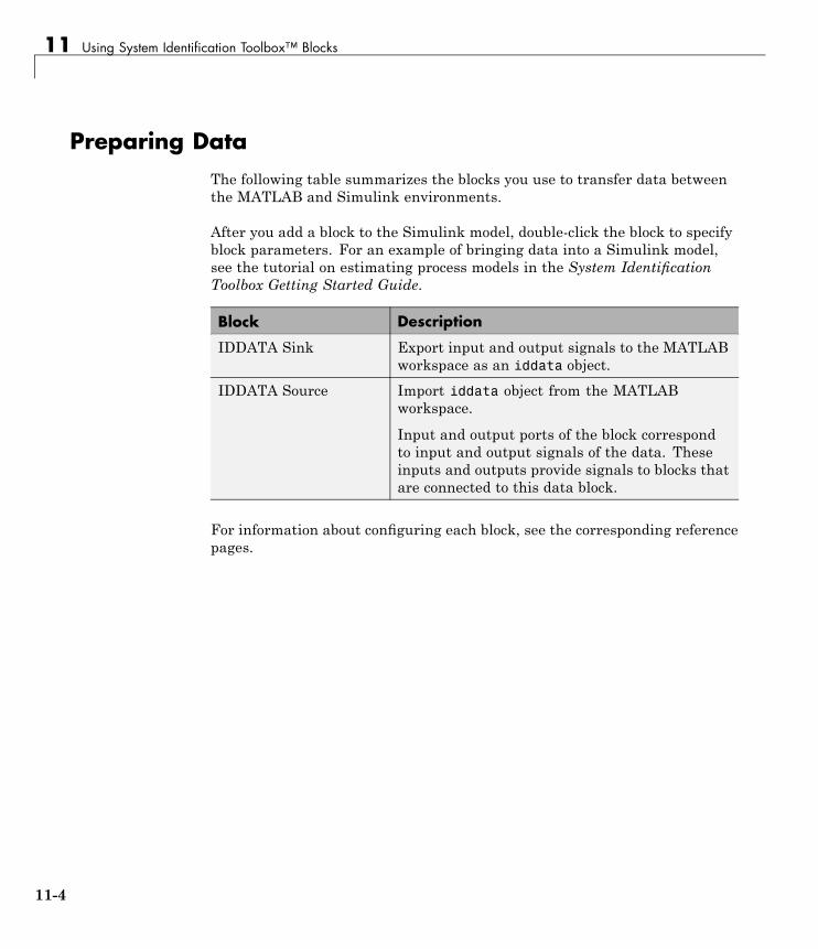
11 Using System Identification Toolbox™ Blocks
Preparing DataThe following table summarizes the blocks you use to transfer data betweenthe MATLAB and Simulink environments.
After you add a block to the Simulink model, double-click the block to specifyblock parameters. For an example of bringing data into a Simulink model,see the tutorial on estimating process models in the System IdentificationToolbox Getting Started Guide.
Block Description
IDDATA Sink Export input and output signals to the MATLABworkspace as an iddata object.
IDDATA Source Import iddata object from the MATLABworkspace.
Input and output ports of the block correspondto input and output signals of the data. Theseinputs and outputs provide signals to blocks thatare connected to this data block.
For information about configuring each block, see the corresponding referencepages.
11-4

Identifying Linear Models
Identifying Linear ModelsThe following table summarizes the blocks you use to estimate modelparameters in a Simulink model during simulation and export the results tothe MATLAB environment.
After you add a block to the model, double-click the block to specify blockparameters.
Block Description
AR Estimator Estimate AR model parameters from time-seriesdata, which has one output and no input.
ARMAX Estimator Estimate ARMAX model parameters frominput/output data.
ARX Estimator Estimate ARX model parameters frominput/output data.
BJ Estimator Estimate BJ model parameters from input/outputdata.
OE Estimator Estimate OE model parameters frominput/output data.
PEM Estimator Estimate ARX, ARMAX, Box-Jenkins, andOutput-Error models (idpoly objects) fromsingle-input and single output data using generalprediction-error method.
For information about configuring each block, see the corresponding referencepages.
11-5
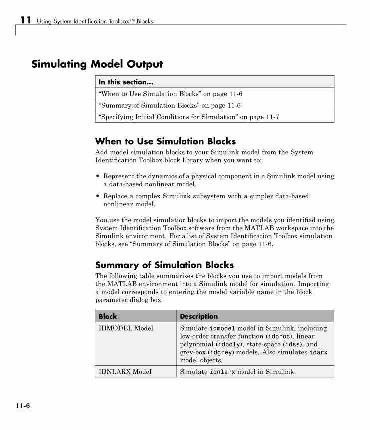
11 Using System Identification Toolbox™ Blocks
Simulating Model Output
In this section...
“When to Use Simulation Blocks” on page 11-6“Summary of Simulation Blocks” on page 11-6“Specifying Initial Conditions for Simulation” on page 11-7
When to Use Simulation BlocksAdd model simulation blocks to your Simulink model from the SystemIdentification Toolbox block library when you want to:
• Represent the dynamics of a physical component in a Simulink model usinga data-based nonlinear model.
• Replace a complex Simulink subsystem with a simpler data-basednonlinear model.
You use the model simulation blocks to import the models you identified usingSystem Identification Toolbox software from the MATLAB workspace into theSimulink environment. For a list of System Identification Toolbox simulationblocks, see “Summary of Simulation Blocks” on page 11-6.
Summary of Simulation BlocksThe following table summarizes the blocks you use to import models fromthe MATLAB environment into a Simulink model for simulation. Importinga model corresponds to entering the model variable name in the blockparameter dialog box.
Block Description
IDMODEL Model Simulate idmodel model in Simulink, includinglow-order transfer function (idproc), linearpolynomial (idpoly), state-space (idss), andgrey-box (idgrey) models. Also simulates idarxmodel objects.
IDNLARX Model Simulate idnlarx model in Simulink.
11-6

Simulating Model Output
Block Description
IDNLHW Model Simulate idnlhw model in Simulink.IDNLGREY Model Simulate nonlinear ODE (idnlgreymodel object)
in Simulink.
After importing the model into Simulink, use the block parameter dialog boxto specify the initial conditions for simulating that block, as described in“Specifying Initial Conditions for Simulation” on page 11-7. For informationabout configuring each block, see the corresponding reference pages.
Specifying Initial Conditions for SimulationFor accurate simulation of a linear or a nonlinear model, you can use defaultinitial conditions or specify the initial conditions for simulation using theblock parameters dialog box.
Tip Double-click the block after adding it your Simulink model to open theblock parameters dialog box.
Specifying Initial States of Linear ModelsFor linear models, the default initial states are the states computed duringmodel estimation and stored by the InitialStates model property. Foridarx and idpoly models, the default initial states are 0. For idproc, idss,and idgrey models, the InitialStates model property can be nonzero valuesafter model estimation.
Because idss and idgrey models are state-space models, the definition ofinitial states corresponds to the standard definition of states for state-spacerepresentation. For idproc, idpoly, and idarx models, the states are thestates of the corresponding state-space model. For example, suppose you havethe following idpoly model:
m1=idpoly([1 2 1],[2 2]);
The initial states of the previous model correspond to those of the equivalentstate-space model:
11-7
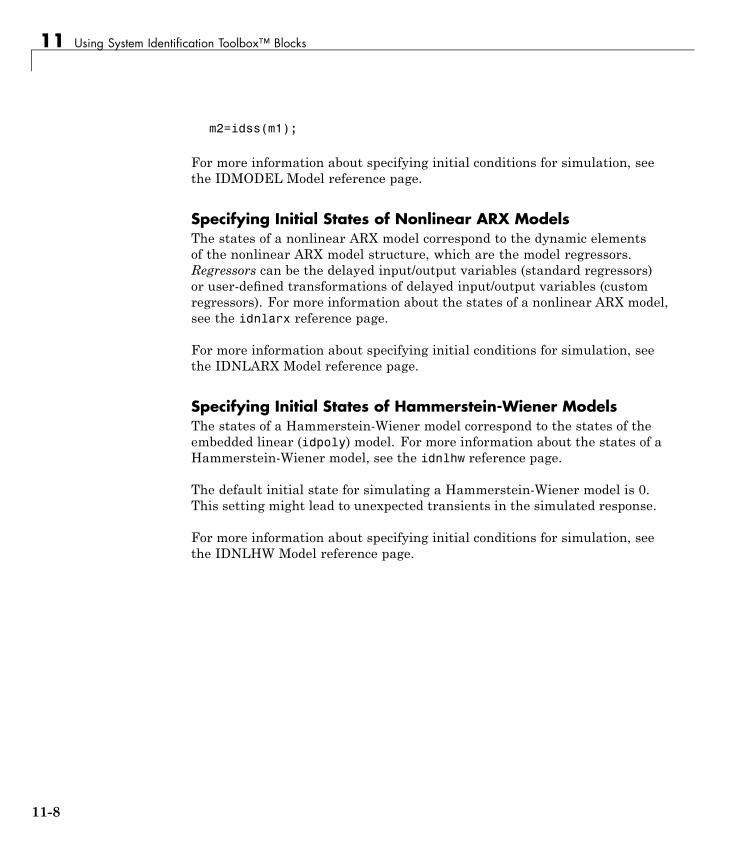
11 Using System Identification Toolbox™ Blocks
m2=idss(m1);
For more information about specifying initial conditions for simulation, seethe IDMODEL Model reference page.
Specifying Initial States of Nonlinear ARX ModelsThe states of a nonlinear ARX model correspond to the dynamic elementsof the nonlinear ARX model structure, which are the model regressors.Regressors can be the delayed input/output variables (standard regressors)or user-defined transformations of delayed input/output variables (customregressors). For more information about the states of a nonlinear ARX model,see the idnlarx reference page.
For more information about specifying initial conditions for simulation, seethe IDNLARX Model reference page.
Specifying Initial States of Hammerstein-Wiener ModelsThe states of a Hammerstein-Wiener model correspond to the states of theembedded linear (idpoly) model. For more information about the states of aHammerstein-Wiener model, see the idnlhw reference page.
The default initial state for simulating a Hammerstein-Wiener model is 0.This setting might lead to unexpected transients in the simulated response.
For more information about specifying initial conditions for simulation, seethe IDNLHW Model reference page.
11-8

Example – Simulating a Model Using Simulink® Software
Example – Simulating a Model Using Simulink SoftwareIn this example, you set the initial states for simulating a model such that thesimulation provides a best fit to measured input-output data.
Suppose you estimate a three-state model M using a multiple-experiment dataset Z, which contains data from five experiments—z1, z2, z3, z4, and z5:
Z = merge(z1,z2,z3,z4,z5);M = n4sid(Z,3);
When a model uses several data sets, the initial-states property stores onlythe estimated states corresponding to the last data set. In this example, M.X0is a vector of length 3 (corresponding to the three states of the model). Thevalues of M.X0 are the estimated state values corresponding to z5.
The following procedure describes how to access the initial states thatcorrespond to z2 for the simulation, where z2 is a portion of the estimationdata Z.
To compare the measured output from experiment z2 with the simulatedoutput:
1 Estimate the initial states using the second experiment as input, that isZ(z2.u), as follows:
X0est = findstates(M,getexp(Z,2))
In this case, getexp(Z,2) gets the data in z2.
2 In the Simulink model window, open the Function Block Parameters dialogbox for the idmodel block.
3 In the idmodel variable field, type M to specify the estimated model.
4 In the Initial states field, type X0est to specify the estimated initial states.
5 Click OK.
Run the simulation to compare the measured output z2.y to the simulatedoutput.
11-9

11 Using System Identification Toolbox™ Blocks
11-10

12
Using the SystemIdentification Tool GUI
• “Steps for Using the System Identification Tool GUI” on page 12-2
• “Starting and Managing GUI Sessions” on page 12-3
• “Managing Models in the GUI” on page 12-9
• “Working with Plots in the System Identification Tool GUI” on page 12-15
• “Customizing the System Identification Tool GUI” on page 12-21
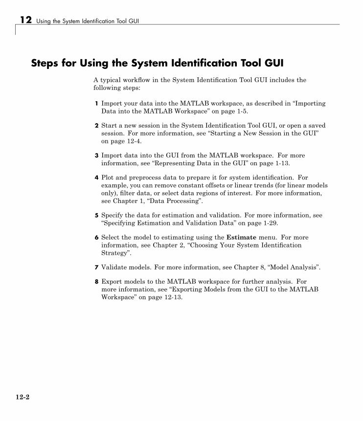
12 Using the System Identification Tool GUI
Steps for Using the System Identification Tool GUIA typical workflow in the System Identification Tool GUI includes thefollowing steps:
1 Import your data into the MATLAB workspace, as described in “ImportingData into the MATLAB Workspace” on page 1-5.
2 Start a new session in the System Identification Tool GUI, or open a savedsession. For more information, see “Starting a New Session in the GUI”on page 12-4.
3 Import data into the GUI from the MATLAB workspace. For moreinformation, see “Representing Data in the GUI” on page 1-13.
4 Plot and preprocess data to prepare it for system identification. Forexample, you can remove constant offsets or linear trends (for linear modelsonly), filter data, or select data regions of interest. For more information,see Chapter 1, “Data Processing”.
5 Specify the data for estimation and validation. For more information, see“Specifying Estimation and Validation Data” on page 1-29.
6 Select the model to estimating using the Estimate menu. For moreinformation, see Chapter 2, “Choosing Your System IdentificationStrategy”.
7 Validate models. For more information, see Chapter 8, “Model Analysis”.
8 Export models to the MATLAB workspace for further analysis. Formore information, see “Exporting Models from the GUI to the MATLABWorkspace” on page 12-13.
12-2

Starting and Managing GUI Sessions
Starting and Managing GUI Sessions
In this section...
“What Is a System Identification Tool Session?” on page 12-3“Starting a New Session in the GUI” on page 12-4“Description of the System Identification Tool Window” on page 12-5“Opening a Saved Session” on page 12-6“Saving, Merging, and Closing Sessions” on page 12-6“Deleting a Session” on page 12-7“Getting Help in the GUI” on page 12-7“Exiting the System Identification Tool GUI” on page 12-8
What Is a System Identification Tool Session?A session represents the total progress of your identification process, includingany data sets and models in the System Identification Tool GUI.
You can save a session to a file with a .sid extension. For example, you cansave different stages of your progress as different sessions so that you canrevert to any stage by simply opening the corresponding session.
To start a new session, see “Starting a New Session in the GUI” on page 12-4.
For more information about the steps for using the System Identification ToolGUI, see “Steps for Using the System Identification Tool GUI” on page 12-2.
12-3

12 Using the System Identification Tool GUI
Starting a New Session in the GUITo start a new session in the System Identification Tool GUI, type thefollowing command in the MATLAB Command Window:
ident
Alternatively, you can start a new session by selectingStart > Toolboxes > System Identification > System IdentificationTool GUI in the MATLAB desktop. This action opens the SystemIdentification Tool GUI.
Note Only one session can be open at a time.
You can also start a new session by closing the current session usingFile > Close session. This toolbox prompts you to save your current sessionif it is not already saved.
12-4

Starting and Managing GUI Sessions
Description of the System Identification Tool WindowThe following figure describes the different areas in the System IdentificationTool GUI.
(����1�� ������1�� �
"����$�������������������������&
"����$�������������������������&
The layout of the window organizes tasks and information from left to right.This organization follows a typical workflow, where you start in the top-leftcorner by importing data into the System Identification Tool GUI using
12-5

12 Using the System Identification Tool GUI
the Import data menu and end in the bottom-right corner by plotting thecharacteristics of your estimated model on model plots. For more informationabout using the System Identification Tool GUI, see “Steps for Using theSystem Identification Tool GUI” on page 12-2.
The Data Board area, located below the Import data menu in the SystemIdentification Tool GUI, contains rectangular icons that represent the datayou imported into the GUI.
The Model Board, located to the right of the <–Preprocess menu in theSystem Identification Tool GUI, contains rectangular icons that represent themodels you estimated or imported into the GUI. You can drag and drop modelicons in the Model Board into open dialog boxes.
Opening a Saved SessionYou can open a previously saved session using the following syntax:
ident(session,path)
session is the file name of the session you want to open and path is thelocation of the session file. Session files have the extension .sid. When thesession file in on the matlabpath, you can omit the path argument.
If the System Identification Tool GUI is already open, you can open a sessionby selecting File > Open session.
Note If there is data in the System Identification Tool GUI, you mustclose the current session before you can open a new session by selectingFile > Close session.
Saving, Merging, and Closing SessionsThe following table summarizes the menu commands for saving, merging, andclosing sessions in the System Identification Tool GUI.
12-6

Starting and Managing GUI Sessions
Task Command Comment
Close thecurrentsession andstart a newsession.
File > Close session You are prompted to save thecurrent session before closingit.
Merge thecurrentsession witha previouslysaved session.
File > Merge session You must start a new sessionand import data or modelsbefore you can select to mergeit with a previously savedsession. You are promptedto select the session file tomerge with the current. Thisoperation combines the dataand the models of both sessionsin the current session.
Save thecurrentsession.
File > Save Useful for saving the sessionrepeatedly after you havealready saved the session once.
Save thecurrentsession undera new name.
File > Save As Useful when you want to saveyour work incrementally. Thiscommand lets you revert to aprevious stage, if necessary.
Deleting a SessionTo delete a saved session, you must delete the corresponding session file.
Getting Help in the GUISystem Identification Tool GUI provides online help topics that you canaccess from the Help menu.
Contextual help is available from each dialog box by clicking the Help buttonin the dialog box.
12-7
12 Using the System Identification Tool GUI
Exiting the System Identification Tool GUITo exit the System Identification Tool GUI, click Exit in the bottom-leftcorner of the window.
Tip Alternatively, select File > Exit System Identification Tool GUI.
12-8
Managing Models in the GUI
Managing Models in the GUI
In this section...
“Importing Models into the GUI” on page 12-9“Viewing Model Properties” on page 12-10“Renaming Models and Changing Display Color” on page 12-11“Organizing Model Icons” on page 12-11“Deleting Models in the GUI” on page 12-12“Exporting Models from the GUI to the MATLAB Workspace” on page 12-13
Importing Models into the GUIYou can import System Identification Toolbox models from the MATLABworkspace into the System Identification Tool GUI. If you have ControlSystem Toolbox software, you can also import any models (LTI objects) youcreated using this toolbox.
The following procedure assumes that you begin with the SystemIdentification Tool GUI already open. If this window is not open, type thefollowing command at the prompt:
ident
To import models into the System Identification Tool GUI:
1 In the System Identification Tool GUI, select Import from the Importmodels list to open the Import Model Object dialog box.
2 In the Enter the name field, type the name of a model object. Press Enter.
3 (Optional) In the Notes field, type any notes you want to store with thismodel.
4 Click Import.
5 Click Close to close the Import Model Object dialog box.
12-9
12 Using the System Identification Tool GUI
Viewing Model PropertiesYou can get information about each model in the System Identification ToolGUI by right-clicking the corresponding model icon.
The Data/model Info dialog box opens. This dialog box describes the contentsand the properties of the corresponding model. It also displays any associatednotes and the command-line equivalent of the operations you used to createthis model.
Tip To view or modify properties for several models, keep this windowopen and right-click each model in the System Identification Tool GUI. TheData/model Info dialog box updates when you select each model.
12-10

Managing Models in the GUI
Renaming Models and Changing Display ColorYou can rename a model and change its display color by double-clicking themodel icon in the System Identification Tool GUI.
The Data/model Info dialog box opens. This dialog box describes both thecontents and the properties of the model. The object description area displaysthe syntax of the operations you used to create the model in the GUI.
To rename the model, enter a new name in theModel name field.
You can also specify a new display color using three RGB values in the Colorfield. Each value is between 0 to 1 and indicates the relative presence ofred, green, and blue, respectively. For more information about specifyingdefault data color, see “Customizing the System Identification Tool GUI” onpage 12-21.
Tip As an alternative to using three RGB values, you can enter any one ofthe following letters in single quotes:
'y' 'r' 'b' 'c' 'g' 'm' 'k'
These strings represent yellow, red, blue, cyan, green, magenta, and black,respectively.
Finally, you can enter comments about the origin and state of the model inthe Diary And Notes area.
To view model properties in the MATLAB Command Window, click Present.
Organizing Model IconsYou can rearrange model icons in the System Identification Tool GUI bydragging and dropping the icons to empty Model Board rectangles.
Note You cannot drag and drop a model icon into the data area on the left.
12-11

12 Using the System Identification Tool GUI
When you need additional space for organizing model icons, selectOptions > Extra model/data board in the System Identification Tool GUI.This action opens an extra session window with blank rectangles. The newwindow is an extension of the current session and does not represent a newsession.
Tip When you import or estimate models and there is insufficient space forthe icons, an additional session window opens automatically.
You can drag and drop model icons between the main System IdentificationTool GUI and any extra session windows.
Type comments in the Notes field to describe the models. When you save asession, as described in “Saving, Merging, and Closing Sessions” on page 12-6,all additional windows and notes are also saved.
Deleting Models in the GUITo delete models in the System Identification Tool GUI, drag and drop thecorresponding icon into Trash. Moving items to Trash does not permanentlydelete these items.
12-12
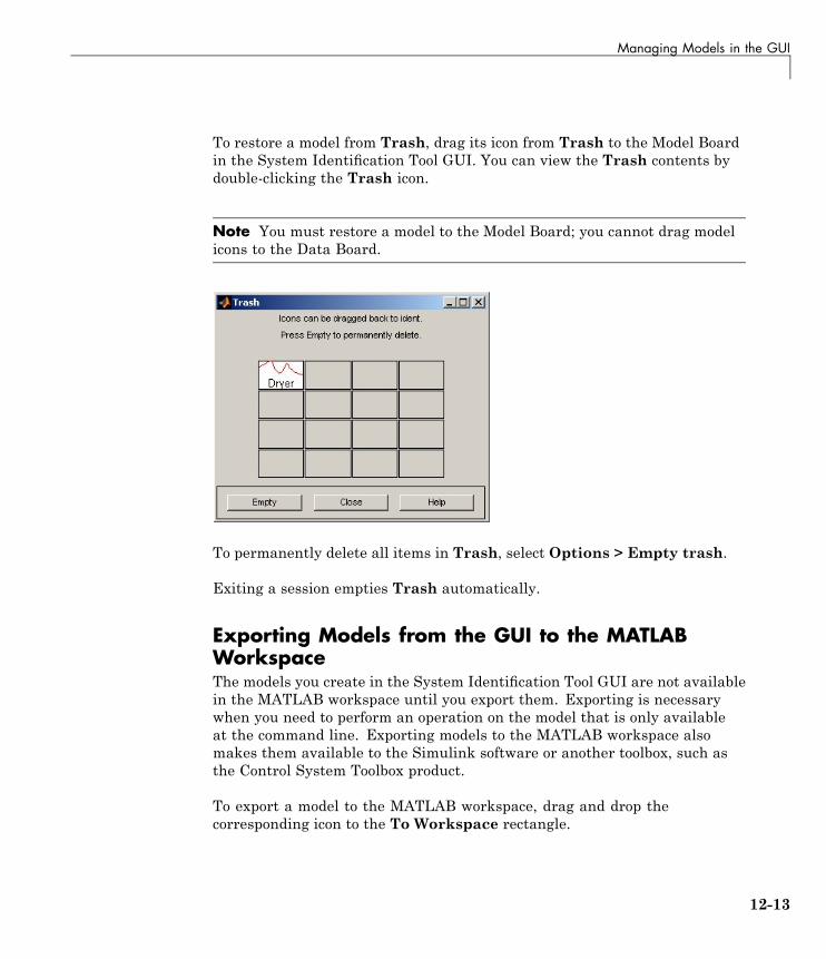
Managing Models in the GUI
To restore a model from Trash, drag its icon from Trash to the Model Boardin the System Identification Tool GUI. You can view the Trash contents bydouble-clicking the Trash icon.
Note You must restore a model to the Model Board; you cannot drag modelicons to the Data Board.
To permanently delete all items in Trash, select Options > Empty trash.
Exiting a session empties Trash automatically.
Exporting Models from the GUI to the MATLABWorkspaceThe models you create in the System Identification Tool GUI are not availablein the MATLAB workspace until you export them. Exporting is necessarywhen you need to perform an operation on the model that is only availableat the command line. Exporting models to the MATLAB workspace alsomakes them available to the Simulink software or another toolbox, such asthe Control System Toolbox product.
To export a model to the MATLAB workspace, drag and drop thecorresponding icon to the To Workspace rectangle.
12-13

12 Using the System Identification Tool GUI
When you export models to the MATLAB workspace, the resulting variableshave the same name as in the System Identification Tool GUI.
12-14
Working with Plots in the System Identification Tool GUI
Working with Plots in the System Identification Tool GUI
In this section...
“Identifying Data Sets and Models on Plots” on page 12-15“Changing and Restoring Default Axis Limits” on page 12-16“Selecting Measured and Noise Channels in Plots” on page 12-18“Grid, Line Styles, and Redrawing Plots” on page 12-19“Opening a Plot in a MATLAB Figure Window” on page 12-19“Printing Plots” on page 12-20
Identifying Data Sets and Models on PlotsYou can identify data sets and models on a plot by color: the color of the linein the data or model icon in the System Identification Tool GUI matches theline color on the plots.
You can also display data tips for each line on the plot. How you display thedata tip depends on whether the zoom feature is enabled:
• When zoom is enabled, press and hold down Shift, and click the desiredcurve to display the data tip.
• When zoom is disabled, click a plot curve and hold down the mouse buttonto display the data tip.
For more information about enabling zoom, see “Magnifying Plots” on page12-16.
The following figure shows an example of a data tip, which contains the nameof the data set and the coordinates of the data point.
12-15
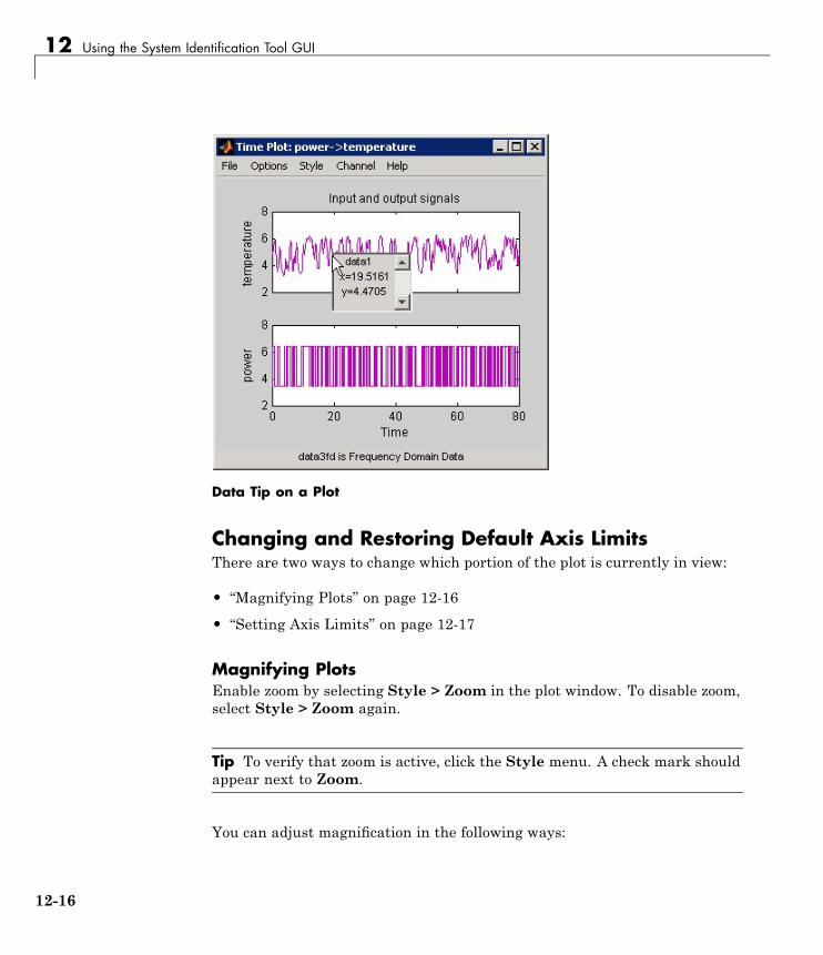
12 Using the System Identification Tool GUI
Data Tip on a Plot
Changing and Restoring Default Axis LimitsThere are two ways to change which portion of the plot is currently in view:
• “Magnifying Plots” on page 12-16
• “Setting Axis Limits” on page 12-17
Magnifying PlotsEnable zoom by selecting Style > Zoom in the plot window. To disable zoom,select Style > Zoom again.
Tip To verify that zoom is active, click the Style menu. A check mark shouldappear next to Zoom.
You can adjust magnification in the following ways:
12-16

Working with Plots in the System Identification Tool GUI
• To zoom in default increments, left-click the portion of the plot you want tocenter in the plot window.
• To zoom in on a specific region, click and drag a rectangle that identifiesthe region for magnification. When you release the mouse button, theselected region is displayed.
• To zoom out, right-click on the plot.
Note To restore the full range of the data in view, selectOptions > Autorange in the plot window.
Setting Axis LimitsYou can change axis limits for the vertical and the horizontal axes of the inputand output channels that are currently displayed on the plot.
1 Select Options > Set axes limits to open the Limits dialog box.
2 Specify a new range for each axis by editing its lower and upper limits. Thelimits must be entered using the format [LowerLimit UpperLimit]. ClickApply. For example:
[0.1 100]
Note To restore full axis limits, select the Auto check box to the rightof the axis name, and click Apply.
3 To plot data on a linear scale, clear the Log check box to the right of theaxis name, and click Apply.
Note To revert to base-10 logarithmic scale, select the Log check box tothe right of the axis name, and click Apply.
4 Click Close.
12-17

12 Using the System Identification Tool GUI
Note To view the entire data range, select Options > Autorange in theplot window.
Selecting Measured and Noise Channels in PlotsModel inputs and outputs are called channels. When you create a plot ofa multivariable input-output data set or model, the plot only shows oneinput-output channel pair at a time. The selected channel names aredisplayed in the title bar of the plot window.
Note When you select to plot multiple data sets, and each data set containsseveral input and output channels, the Channel menu lists channel pairsfrom all data sets.
You can select a different input-output channel pair from the Channel menuin any System Identification Toolbox plot window.
The Channel menu uses the following notation for channels: u1->y2 meansthat the plot displays a transfer function from input channel u1 to outputchannel y2. System Identification Toolbox estimates as many noise sources asthere are output channels. In general, e@ynam indicates that the noise sourcecorresponds to the output with name ynam.
For example, e@y3->y1 means that the transfer function from the noisechannel (associated with y3) to output channel y2 is displayed. For moreinformation about noise channels, see “Subreferencing Measured and NoiseModels” on page 3-120.
Tip When you import data into the System Identification Tool GUI, it ishelpful to assign meaningful channel names in the Import Data dialog box.For more information about importing data, see “Representing Data in theGUI” on page 1-13.
12-18

Working with Plots in the System Identification Tool GUI
Grid, Line Styles, and Redrawing PlotsThere are several Style options that are common to all plot types. Theseinclude the following:
• “Grid Lines” on page 12-19
• “Solid or Dashed Lines” on page 12-19
• “Plot Redrawing” on page 12-19
Grid LinesTo toggle showing or hiding grid lines, select Style > Grid.
Solid or Dashed LinesTo display currently visible lines as a combination of solid, dashed, dotted,and dash-dotted line style, select Style > Separate linestyles.
To display all solid lines, select Style > All solid lines. This choice is thedefault.
All line styles match the color of the corresponding data or model icon inthe System Identification Tool GUI.
Plot RedrawingTo specify that the plot be redrawn when you add another data set or modelto the plot, select Style > Erasemode normal. This choice is the defaultsetting.
To avoid redrawing the entire plot when you add another data set or model tothe plot, select Style > Erasemode xor. Although this selection results infaster response, it might also produce poor plot quality.
Opening a Plot in a MATLAB Figure WindowThe MATLAB Figure window provides editing and printing commands forplots that are not available in the System Identification Toolbox plot window.To take advantage of this functionality, you can first create a plot in the
12-19

12 Using the System Identification Tool GUI
System Identification Tool GUI, and then open it in a MATLAB Figurewindow to fine-tune the display.
After you create the plot, as described in “Plotting Models in the GUI” on page8-5, select File > Copy figure in the plot window. This command opens theplot in a MATLAB Figure window.
Printing PlotsTo print a System Identification Toolbox plot, select File > Print in the plotwindow. In the Print dialog box, select the printing options and click OK.
12-20

Customizing the System Identification Tool GUI
Customizing the System Identification Tool GUI
In this section...
“Types of GUI Customization” on page 12-21“Displaying Warnings While You Work” on page 12-21“Saving Session Preferences” on page 12-21“Modifying idlayout.m” on page 12-22
Types of GUI CustomizationThe System Identification Tool GUI lets you customize the window behaviorand appearance. For example, you can set the size and position of specificdialog boxes and modify the appearance of plots.
You can save the session to save the customized GUI state.
Advanced users might choose to edit the M-file that controls default settings,as described in “Modifying idlayout.m” on page 12-22.
Displaying Warnings While You WorkIn the System Identification Tool GUI, select Options > Warnings to displayinformational dialog boxes while you work. Verify that a check mark appearsto the right of Warnings.
To stop warnings from being displayed during your session, selectOptions > Warnings and clear the check mark.
Saving Session PreferencesUse Options > Save preferences to save the current state of the SystemIdentification Tool GUI. This command saves the following settings to apreferences file, idprefs.mat:
• Size and position of the System Identification Tool GUI
• Sizes and positions of dialog boxes
12-21

12 Using the System Identification Tool GUI
• Four recently used sessions
• Plot options, such as line styles, zoom, grid, and whether the input isplotted using zero-order hold or first-order hold between samples
You can only edit idprefs.mat by changing preferences in the GUI.
The idprefs.mat file is located in the same directory as startup.m, bydefault. To change the location where your preferences are saved, use themidprefs command with the new path as the argument. For example:
midprefs('c:\matlab\toolbox\local\')
You can also type midprefs and browse to the desired directory.
To restore the default preferences, select Options > Default preferences.
Modifying idlayout.mAdvanced users might want to customize the default plot options by editingidlayout.m.
To customize idlayout.m defaults, save a copy of idlayout.m to a folder inyour matlabpath just above the ident directory level.
Caution Do not edit the original file to avoid overwriting the idlayout.mdefaults shipped with the product.
You can customize the following plot options in idlayout.m:
• Order in which colors are assigned to data and model icons
• Line colors on plots
• Axis limits and tick marks
• Plot options, set in the plot menus
• Font size
12-22
Customizing the System Identification Tool GUI
Note When you save preferences using Options > Save preferencesto idprefs.mat, these preferences override the defaults in idlayout.m.To give idlayout.m precedence every time you start a new session, selectOptions > Default preferences.
12-23

12 Using the System Identification Tool GUI
12-24

Index
IndexAactive
model in GUI 8-5advice
for data 1-84for models 8-7
AIC 8-61definition 8-62
Akaike’s Final Prediction Error (FPE) 8-61Akaike’s Information Criterion (AIC) 8-61Algorithm property 2-15algorithms for estimation
recursive 7-6spectral models 3-5
aliasing effects 1-103AR 6-7ARMA 6-7ARMAX 3-44ARX 3-44ARX Model Structure Selection window 3-55
Bbest fit
definition 8-11negative value 8-12
BJ model. See Box-Jenkins modelBode plot 8-34Box-Jenkins model 3-44Burg’s method 6-11
Cc2d 3-112canonical parameterization 3-91
complex data 1-131concatenating
iddata objects 1-65idfrd objects 1-71models 3-124
confidence intervalimpulse response plot 8-29model output plot 8-13noise spectrum plot 8-41residual plot 8-18step response plot 8-29
confidence interval on plots 8-65constructor 2-12continuous-time models
supported 2-7continuous-time process models 3-22Control System Toolbox
combining model objects 10-6converting models to LTI objects 10-4for compensator design 10-3LTI Viewer 10-5reducing model order 10-3
correlation analysis 3-14covariance 8-64CovarianceMatrix 8-64cra 3-16cross-validation 8-4custom network 4-25
DD matrix 3-89d2c 3-112d2d 3-112
Index-1

Index
datacreating iddata object 1-47creating idfrd object 1-67creating subsets 1-31detrending 1-94exporting to MATLAB workspace 1-45filter 1-107frequency-domain 1-8frequency-response 1-10importing into System Identification Tool
GUI 1-13managing in GUI 1-13merging 1-33missing data 1-90multiexperiment data 1-33outliers 1-91plotting 1-75renaming in GUI 1-41resampling 1-100sampling interval 1-28segmentation 7-14selecting 1-86simulating 1-115supported types 1-5time-domain 1-6time-series 1-7transforming domain 1-119viewing properties in GUI 1-40
Data Board 12-6arranging icons 1-43deleting icons 1-44
data tip 12-15dead time 3-41dead zone 4-25delay
estimating for polynomial models 3-49detrending data 1-94discrete-time models
supported 2-8
Eestimating models
black-box polynomial 3-41commands 2-9frequency response 3-2Hammerstein-Wiener 4-15linear grey-box 5-6nonlinear ARX 4-4nonlinear grey-box 5-16process models 3-22recursive estimation 7-2state-space 3-73time-series 6-1transient response 3-14uncertainty 8-64
EstimationInfo property 2-16etfe
algorithm 3-5export
data to MATLAB workspace 1-45model to MATLAB workspace 12-13
Ffiltering data 1-107forgetting factor algorithm 7-10FPE 8-61free parameterization 3-84frequency resolution 3-6frequency response
estimating in the GUI 3-3etfe 3-5spa 3-5spafdr 3-5
frequency-domain data 1-8frequency-response data 1-10frequency-response function 3-9frequency-response plot 8-32
Bode plot 8-35Nyquist plot 8-38
Index-2
Index
HHammerstein-Wiener models 4-15Hammerstein-Wiener plot 8-56
Iidarx 2-13iddata
concatenating 1-65creating 1-47subreferencing 1-55
ident 12-4idfrd
concatenating 1-71creating 1-67model 2-13subreferencing 1-70
idgrey 2-13idlayout.m 12-22idnlarx 2-13idnlgrey 2-13idnlhw 2-13idpoly 2-13idproc 2-13idss 2-13importing
data into System Identification ToolGUI 1-13
impulse responsecomputing values 3-18confidence interval 8-29definition 3-14estimating in the GUI 3-15impulse 3-16
impulse-response plot 8-24independence test 8-16initial states for simulation and prediction 9-8
KK matrix 3-89Kalman filter algorithm 7-8
Llinear grey-box models 5-6linear models
extracting numerical data 3-108transforming between continuous and
discrete time 3-112transforming between structures 3-117
LTI Viewer 10-5
MMDL 3-54merging
data 1-33models 3-128
methods 2-11missing data 1-90
Index-3
Index
modelblack-box polynomial 3-41estimating frequency response 3-2estimating process model 3-22estimating transient response 3-14exporting to MATLAB workspace 12-13grey-box estimation 5-1Hammerstein-Wiener estimation 4-15importing into GUI 12-9linear grey-box estimation 5-6managing in GUI 12-9nonlinear ARX estimation 4-4nonlinear black-box estimation 4-1nonlinear grey-box estimation 5-16ordinary difference equation 5-1ordinary differential equation 5-1plotting 8-4predict output 9-7properties 2-14recursive estimation 7-2reducing order using balred 10-3reducing order using pole-zero plot 8-51refining linear parametric 3-103refining nonlinear black-box 4-28renaming in GUI 12-11state-space 3-73time-series 6-1uncertainty 8-64validating 8-2viewing properties in GUI 12-10
Model Board 12-6arranging icons 12-11deleting icons 12-12
model objectconcatenating 3-124definition 2-11instantiating 2-12merging 3-128methods 2-11properties 2-11 2-14types of 2-13
model orderdefinition 3-41estimating for polynomial models 3-49estimating for state-space 3-79too high or too low 8-67
Model Order Selection window 3-83model output
confidence interval 8-13model output plot 8-8model properties
accessing 2-17help on 2-19specifying 2-16
multiexperiment data 1-33
Nneural network 4-25noise
converting to measured channels 3-122evidence in estimated model 8-69subreferencing 3-120
noise spectrumconfidence interval 8-41
noise spectrum plot 8-40nonlinear ARX models 4-4nonlinear ARX plot 8-52nonlinear grey-box models 5-16nonlinear models 4-1nonlinearities 4-25nonlinearity estimators 4-25
troubleshooting 8-68
Index-4
Index
normalized gradient algorithm 7-11
OOE model. See Output-Error modeloffset levels 1-94order. See model orderoutliers 1-91Output-Error model 3-44
Ppem
for polynomial models 3-61for process models 3-29for state-space models 3-87
periodogrametfe for time series 6-5
physical equilibrium 1-94piece-wise linear 4-25plot
copy to MATLAB Figure window 12-19data 1-75data tip 12-15in LTI Viewer 10-5models 8-4models in the GUI 8-5print 12-20selecting noise channels 12-18
pole-zero cancelation 8-51pole-zero plot 8-47polynomial models 3-41
estimating order 3-49for time-series 6-7
polynomial nonlinearity 4-25predicting model output 9-1
initial states 9-8prediction 9-7
print plot 12-20process model 3-22
definition 3-22properties
for models 2-14
Rrecursive estimation 7-2reducing model order
using balred 10-3using pole-zero plot 8-51
refining modelslinear 3-104linear parametric 3-103nonlinear 4-28nonlinear black-box 4-28using pem 3-105 4-29
renaming data 1-41resampling data 1-100
avoiding aliasing 1-103residual analysis
confidence interval 8-18plot 8-16
residualsplotting using the System Identification
Tool 8-21Rissanen’s Minimum Description Length
(MDL) 3-54robust criterion
for outliers 1-91
Ssampling interval 1-28saving session preferences 12-21segmentation of data 7-14selecting data 1-86
Index-5

Index
sessiondefinition 12-3managing in GUI 12-3preferences 12-21starting 12-4
sigmoid network 4-25simulating data 1-115simulating model output 9-1
initial states 9-8Simulink 11-2slident 11-3spa
algorithm 3-5spafdr
algorithm 3-5spectral analysis 3-2
algorithm 3-5frequency resolution 3-6spectrum normalization 3-11
spectrum normalization 3-11state-space models 3-73
canonical parameterization 3-91estimating order 3-79for time series 6-12free parameterization 3-84structured parameterization 3-93supported parameterization 3-78
step responsecomputing values 3-18confidence interval 8-29definition 3-14estimating in the GUI 3-15step 3-16
step-response plot 8-24structured parameterization 3-93
subreferencingiddata objects 1-55idfrd objects 1-70model channels 3-119model noise channels 3-120models 3-119
System Identification Tool GUIcustomizing 12-21exiting 12-8help 12-7open 12-4organizing icons 1-43 12-11plots 12-15window 12-5workflow 12-2
System Identification Toolbox blocks 11-2for data 11-4for model identification 11-5for simulating models 11-6open 11-3
Ttime-domain data 1-6time-series data 1-7time-series models 6-1transforming data domain 1-119Trash 1-44 12-12tree partition 4-25troubleshooting models 8-67
complicated nonlinearities 8-71high noise content 8-69missing inputs 8-70model order 8-67nonlinearity estimators 8-68unstable models 8-69
Index-6

Index
Uuncertainty of models 8-64
confidence interval on plots 8-65covariance 8-64
unnormalized gradient algorithm 7-11unstable models 8-69
Vvalidating models 8-2
comparing model output 8-8residual analysis 8-16troubleshooting 8-67
Validation Data 1-29
Wwarnings 12-21wavelet network 4-25whiteness test 8-16Working Data 1-29
XX0 matrix 3-89
YYule-Walker approach 6-11
Index-7