system identification and estimation in labview
TRANSCRIPT

Telemark University College
Department of Electrical Engineering, Information Technology and Cybernetics
Faculty of Technology, Postboks 203, Kjølnes ring 56, N-3901 Porsgrunn, Norway. Tel: +47 35 57 50 00 Fax: +47 35 57 54 01
System Identification and
Estimation in LabVIEW
HANS-PETTER HALVORSEN, 2011.08.16

i
Preface
This Tutorial will go through the basic principles of System identification and Estimation and how to
implement these techniques in LabVIEW and LabVIEW MathScript.
LabVIEW is a graphical programming language created by National Instruments, while LabVIEW
MathScript is an add-on to LabVIEW. LabVIEW MathScript has similar syntax as, e.g., MATLAB.
LabVIEW MathScript may be used as a separate part (and can be considered as a miniature version of
MATLAB) or be integrated into the graphical LabVIEW code using the MathScript Node.
The following methods will be discussed:
State Estimation:
Kalman Filter
Observers
Parameter Estimation:
Least Square Method (LS)
System Identification
Sub-space methods/Black-Box methods
Polynomial Model Estimation: ARX/ARMAX model Estimation
Software
You need the following software in this Tutorial:
LabVIEW
LabVIEW MathScript RT Module (LabVIEW MathScript)
LabVIEW Control Design and Simulation Module
LabVIEW System Identification Toolkit
“LabVIEW Control Design and Simulation Module” has functionality for creating Kalman Filters and
Observers, while “LabVIEW System Identification Toolkit” has functionality for System identification.

ii
Table of Contents
Preface ................................................................................................................................................ i
Table of Contents................................................................................................................................ ii
1 Introduction to LabVIEW and LabVIEW MathScript ..................................................................... 5
1.1 LabVIEW .............................................................................................................................. 5
1.2 LabVIEW MathScript ............................................................................................................ 6
2 LabVIEW Control and Simulation Module ................................................................................... 9
3 Model Creation in LabVIEW ...................................................................................................... 11
3.1 State-space Models ........................................................................................................... 12
3.2 Transfer functions ............................................................................................................. 15
3.2.1 commonly used transfer functions ............................................................................. 17
4 Introduction to System identification and Estimation ............................................................... 24
5 State Estimation with Kalman Filter in LabVIEW........................................................................ 26
5.1 State-Space model ............................................................................................................. 27
5.2 Observability ..................................................................................................................... 29
5.3 Introduction to the State Estimator ................................................................................... 31
5.4 State Estimation ................................................................................................................ 37
5.5 LabVIEW Kalman Filter Implementations ........................................................................... 38
6 Create your own Kalman Filter from Scratch ............................................................................. 44
6.1 The Kalman Filter Algorithm .............................................................................................. 44
6.2 Examples ........................................................................................................................... 45
7 Overview of Kalman Filter functions in LabVIEW ....................................................................... 49
7.1 Control Design palette ....................................................................................................... 49
7.1.1 State Feedback Design subpalette .............................................................................. 49
7.1.2 Implementation subpalette........................................................................................ 50
iii Table of Contents
Tutorial: System Identification and Estimation in LabVIEW
7.2 Simulation palette ............................................................................................................. 51
7.2.1 Estimation subpalette ................................................................................................ 51
8 State Estimation with Observers in LabVIEW ............................................................................ 54
8.1 State-Space model ............................................................................................................. 54
8.2 Eigenvalues ....................................................................................................................... 56
8.3 Observer Gain ................................................................................................................... 57
8.4 Observability ..................................................................................................................... 58
8.5 Examples ........................................................................................................................... 59
9 Overview of Observer functions ............................................................................................... 64
9.1 Control Design palette ....................................................................................................... 64
9.1.1 State Feedback Design subpalette .............................................................................. 64
9.1.2 Implementation subpalette........................................................................................ 65
9.2 Simulation palette ............................................................................................................. 66
9.2.1 Estimation subpalette ................................................................................................ 66
10 System Identification in LabVIEW ............................................................................................. 69
10.1 Parameter Estimation with Least Square Method (LS)........................................................ 70
10.2 System Identification using Sub-space methods/Black-Box methods ................................. 73
10.3 System Identification using Polynomial Model Estimation: ARX/ARMAX model Estimation 74
10.4 Generate model Data ........................................................................................................ 75
10.4.1 Excitation signals........................................................................................................ 77
11 Overview of System Identification functions ............................................................................. 80
12 System Identification Example .................................................................................................. 85

4
Part I: Introduction

5
1 Introduction to LabVIEW and
LabVIEW MathScript
In this Tutorial we will use LabVIEW and some of the add-on modules available for LabVIEW.
LabVIEW
LabVIEW MathScript RT Module
LabVIEW Control Design and Simulation Module
LabVIEW System Identification Toolkit
1.1 LabVIEW
LabVIEW (short for Laboratory Virtual Instrumentation Engineering Workbench) is a platform and
development environment for a visual programming language from National Instruments. The
graphical language is named "G". LabVIEW is commonly used for data acquisition, instrument
control, and industrial automation. The code files have the extension “.vi”, which is an abbreviation
for “Virtual Instrument”. LabVIEW offers lots of additional Add-ons and Toolkits.
For more information about LabVIEW, please read the Tutorial “Introduction to LabVIEW”.
6
Introduction to LabVIEW and LabVIEW MathScript
Tutorial: System Identification and Estimation in LabVIEW
I also recommend you visit my Blog: http://home.hit.no/~hansha/ and visit National Instruments at
www.ni.com.
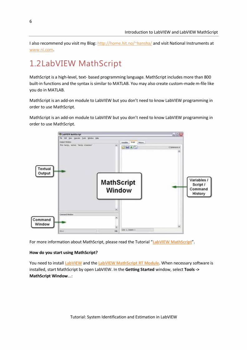
1.2 LabVIEW MathScript
MathScript is a high-level, text- based programming language. MathScript includes more than 800
built-in functions and the syntax is similar to MATLAB. You may also create custom-made m-file like
you do in MATLAB.
MathScript is an add-on module to LabVIEW but you don’t need to know LabVIEW programming in
order to use MathScript.
MathScript is an add-on module to LabVIEW but you don’t need to know LabVIEW programming in
order to use MathScript.
For more information about MathScript, please read the Tutorial “LabVIEW MathScript”.
How do you start using MathScript?
You need to install LabVIEW and the LabVIEW MathScript RT Module. When necessary software is
installed, start MathScript by open LabVIEW. In the Getting Started window, select Tools ->
MathScript Window...:

7
Introduction to LabVIEW and LabVIEW MathScript
Tutorial: System Identification and Estimation in LabVIEW
For more information about MathScript, please read the Tutorial “LabVIEW MathScript”.
MathScript Node:
You may also use MathScript Code directly inside and combined with you graphical LabVIEW code,
for this you use the “MathScript Node”. With the “MathScript Node” you can combine graphical and
textual code within LabVIEW. The figure below shows the “MathScript Node” on the block diagram,
represented by the blue rectangle. Using “MathScript Nodes”, you can enter .m file script text
directly or import it from a text file.
You can define named inputs and outputs on the MathScript Node border to specify the data to
transfer between the graphical LabVIEW environment and the textual MathScript code.
You can associate .m file script variables with LabVIEW graphical programming, by wiring Node inputs
and outputs. Then you can transfer data between .m file scripts with your graphical LabVIEW

8
Introduction to LabVIEW and LabVIEW MathScript
Tutorial: System Identification and Estimation in LabVIEW
programming. The textual .m file scripts can now access features from traditional LabVIEW graphical
programming.
The MathScript Node is available from LabVIEW from the Functions Palette: Mathematics → Scripts
& Formulas
If you click Ctrl+H you get help about the MathScript Node:
Click “Detailed help” in order to get more information about the MathScript Node.

9
2 LabVIEW Control and Simulation
Module
LabVIEW has several additional modules and Toolkits for Control and Simulation purposes, e.g.,
“LabVIEW Control Design and Simulation Module”, “LabVIEW PID and Fuzzy Logic Toolkit”,
“LabVIEW System Identification Toolkit” and “LabVIEW Simulation Interface Toolkit”. LabVIEW
MathScript is also useful for Control Design and Simulation.
LabVIEW Control Design and Simulation Module
LabVIEW PID and Fuzzy Logic Toolkit
LabVIEW System Identification Toolkit
LabVIEW Simulation Interface Toolkit
Below we see the Control Design & Simulation palette in LabVIEW:
In this Tutorial we will focus on the VIs used for Parameter and State estimation and especially the
use of Observers and Kalman Filter for State estimation.
If you want to learn more about Simulation, Simulation Loop, block diagrams and PID control, etc., I
refer to the Tutorial “Control and Simulation in LabVIEW” This Tutorial is available from
http://home.hit.no/~hansha/ .
In this Tutorial we will need the following sub palettes in the Control Design and Simulation palette:
Control Design
System Identification
Simulation
Below we see the Control Design palette:

10 LabVIEW Control and Simulation Module
Tutorial: System Identification and Estimation in LabVIEW
Below we see the System Identification palette:
Below we see the Simulation palette:
In the next chapters we will go in detail and describe the different sub palettes in these palettes and
explain the functions/Sub VIs we will need for System identification and Estimation.

11
3 Model Creation in LabVIEW
When you have found the mathematical model for your system, the first step is to define/ or create
your model in LabVIEW. Your model can be a Transfer function or a State-space model.
In LabVIEW and the “LabVIEW Control Design and Simulation Module” you can create different
models, such as State-space models and transfer functions, etc.
In the Control Design palette we have several sub palettes that deals with models, these are:
Model Construction
Model Information
Model Conversion
Model Interconnection
Below we go through the different subpalettes and the most used VIs in these palettes.
“Model Construction” Subpalette:
In this palette we have VIs for creating state-space models and transfer functions.

12 Model Creation in LabVIEW
Tutorial: System Identification and Estimation in LabVIEW
→ Use the Model Construction VIs to create linear system models and modify the properties of a
system model. You also can use the Model Construction VIs to save a system model to a file, read a
system model from a file, or obtain a visual representation of a model.
Some of the most used VIs would be:
CD Construct State-Space Model.vi
CD Construct Transfer Function Model.vi
These VIs and some others are explained below.
3.1 State-space Models
Given the following State-space model:
In LabVIEW we use the “CD Construct State-Space Model.vi” to create a State-space model:

13 Model Creation in LabVIEW
Tutorial: System Identification and Estimation in LabVIEW
You may use numeric values in the matrices A,B,C and D or symbolic values by selecting ether
“Numeric” or “Symbolic”:
Numeric Symbolic
Example: Create State-Space model
Block Diagram:
Front Panel:

14 Model Creation in LabVIEW
Tutorial: System Identification and Estimation in LabVIEW
The “CD Draw State-Space Equation.vi” can be used to see a graphical representation of the
State-space model.
Example: Create SISO/MIMO State-Space models
SISO Model (Single Input, Single Output):
SIMO Model (Single Input, Multiple Output):
MISO Model (Multiple Input, Single Output):

15 Model Creation in LabVIEW
Tutorial: System Identification and Estimation in LabVIEW
MIMO Model (Multiple Input, Multiple Output):
[End of Example]
3.2 Transfer functions
Given the following Transfer function:
( )
In LabVIEW we use the “CD Construct Transfer Function Model.vi” to create a Transfer Function:

16 Model Creation in LabVIEW
Tutorial: System Identification and Estimation in LabVIEW
Example: Transfer Function
Block Diagram:
Front Panel:
[End of Example]
Example: Transfer Function with Symbolic values

17 Model Creation in LabVIEW
Tutorial: System Identification and Estimation in LabVIEW
Block Diagram:
Front Panel:
[End of Example]
3.2.1 commonly used transfer functions
For commonly used transfer functions we can use the “CD Construct Special TF Model.vi”:
1.order system:
The transfer function for a 1.order system is as follows:
( )
Where
is the gain
T is the Time constant

18 Model Creation in LabVIEW
Tutorial: System Identification and Estimation in LabVIEW
is the Time delay
Select the polymorphic instance on the “CD Construct Special TF Model.vi”:
2.order system:
The transfer function for a 2.order system is as follows:
( )
. /
Where
is the gain
zeta is the relative damping factor
[rad/s] is the undamped resonance frequency.
Select the polymorphic instance on the “CD Construct Special TF Model.vi”:

19 Model Creation in LabVIEW
Tutorial: System Identification and Estimation in LabVIEW
Time delay as a Pade’ approximation:
Time-delays are very common in control systems. The Transfer function of a time-delay is:
( )
In some situations it is necessary to substitute with an approximation, e.g., the
Padé-approximation:
Select the polymorphic instance on the “CD Construct Special TF Model.vi”:
“Model Information” Subpalette:

20 Model Creation in LabVIEW
Tutorial: System Identification and Estimation in LabVIEW
→ Use the Model Information VIs to obtain or set parameters, data, and names of a system model.
Model information includes properties such as the system delay, system dimensions, sampling time,
and names of inputs, outputs, and states.
“Model Conversion” Subpalette:
→ Use the Model Conversion VIs to convert a system model from one representation to another,
from a continuous-time to a discrete-time model, or from a discrete-time to a continuous-time
model. You also can use the Model Conversion VIs to convert a control design model into a
simulation model or a simulation model into a control design model.
Some of the most used VIs in the “Model Conversion” subpalette are:
CD Convert to State-Space Model.vi
CD Convert to Transfer Function Model.vi
CD Convert Continuous to Discrete.vi
These VIs and some others are explained below.
Convert to State-Space Models:

21 Model Creation in LabVIEW
Tutorial: System Identification and Estimation in LabVIEW
Example: Convert from Transfer function to State-Space model
Block Diagram:
Front Panel:
[End of Example]
Convert to Transfer Functions:

22 Model Creation in LabVIEW
Tutorial: System Identification and Estimation in LabVIEW
Example: Convert from State-Space model to Transfer Function
Block Diagram:
Front Panel:
[End of Example]
Convert Continuous to Discrete Model:
Example: Convert from Continuous State-Space model to Discrete State-Space model
Block Diagram:

23 Model Creation in LabVIEW
Tutorial: System Identification and Estimation in LabVIEW
Front Panel:
[End of Example]
“Model Interconnection” Subpalette:
→ Use the Model Interconnection VIs to perform different types of linear system interconnections.
You can build a large system model by connecting smaller system models together.

24
4 Introduction to System
identification and Estimation
This Tutorial will go through the basic principles of System identification and Estimation and how to
implement these techniques in LabVIEW.
The following methods will be discussed in the next chapters:
State Estimation:
Kalman Filter
Observers
System Identification:
Parameter Estimation and the Least Square Method (LS)
Sub-space methods/Black-Box methods
Polynomial Model Estimation: ARX/ARMAX model Estimation
The next chapters will go through the basic theory and show how it could be implemented in
LabVIEW and MathScript.

25
Part II: Estimation

26
5 State Estimation with Kalman
Filter in LabVIEW
Kalman Filter is a commonly used method to estimate the values of state variables of a dynamic
system that is excited by stochastic (random) disturbances and stochastic (random) measurement
noise.
The Kalman Filter is a state estimator which produces an optimal estimate in the sense that the mean
value of the sum of the estimation errors gets a minimal value.
Below we see a sketch of how a Kalman Filter is working:
The estimator (model of the system) runs in parallel with the system (real system or model). The
measurement(s) is used to update the estimator.
LabVIEW Control Design and Simulation Module have lots of functionality for State Estimation using
Kalman Filters. The functionality will be explained in detail in the next chapters.
Below we see the Discrete Kalman Filter implementation in LabVIEW:

27 State Estimation with Kalman Filter in LabVIEW
Tutorial: System Identification and Estimation in LabVIEW
The Kalman Filter for nonlinear models is called the “Extended Kalman Filter”.
5.1 State-Space model
Given the continuous linear state space-model:
Or given the discrete linear state space-model
LabVIEW:
In LabVIEW we may use the “CD Construct State-Space Model.vi” to create a State-space model:
Note! If you specify a discrete State-space model you have to specify the Sampling Time.
LabVIEW Example: Create a State-space model
Block Diagram:

28 State Estimation with Kalman Filter in LabVIEW
Tutorial: System Identification and Estimation in LabVIEW
The matrices , , and may be defined on the Front Panel like this:
[End of Example]
Discretization:
If you have a continuous model and want to convert it to the discrete model, you may use the VI “CD
Convert Continuous to Discrete.vi” in LabVIEW:
LabVIEW Functions Palette: Control Design & Simulation → Control Design → Model Conversion →
CD Convert Continuous to Discrete.vi
LabVIEW Example: Convert from Continuous to Discrete model
Note! We have to specify the Sampling Time.

29 State Estimation with Kalman Filter in LabVIEW
Tutorial: System Identification and Estimation in LabVIEW
[End of Example]
MathScript:
Use the ss function in MathScript to define your model (or tf if you have a transfer function). Use the
c_to_d function to convert a continuous model to a discrete model.
MathScript Example:
Given the following State-space model:
[ ] [
]⏟
0 1 [
]⏟
, -⏟
0 1
The following MathScript Code creates this model:
c=1;
m=1;
k=1;
A = [0 1; -k/m -c/m];
B = [0; 1/m];
C = [1 0];
ssmodel = ss(A, B, C)
If you want to find the discrete model use the c_to_d function:
Ts=0.1 % Sampling Time
discretemodel = c_to_d(ssmodel, Ts)
[End of Example]
5.2 Observability
A necessary condition for the Kalman Filter to work correctly is that the system for which the states
are to be estimated, is observable. Therefore, you should check for Observability before applying the
Kalman Filter.
The Observability matrix is defined as:
[
]
Where n is the system order (number of states in the State-space model).

30 State Estimation with Kalman Filter in LabVIEW
Tutorial: System Identification and Estimation in LabVIEW
→ A system of order n is observable if is full rank, meaning the rank of is equal to n.
LabVIEW:
The LabVIEW Control Design and Simulation Module have a VI (Observability Matrix.vi) for finding
the Observability matrix and check if a states-pace model is Observable.
LabVIEW Functions Palette: Control Design & Simulation → Control Design → State-Space Model
Analysis → CD Observability Matrix.vi
Note! In LabVIEW is used as a symbol for the Observability matrix.
LabVIEW Example: Check for Observability
[End of Example]
MathScript:
In MathScript you may use the obsvmx function to find the Observability matrix. You may then use
the rank function in order to find the rank of the Observability matrix.
MathScript Example:
The following MathScript Code check for Observability:
% Check for Observability:
O = obsvmx (discretemodel)
r = rank(O)

31 State Estimation with Kalman Filter in LabVIEW
Tutorial: System Identification and Estimation in LabVIEW
[End of Example]
5.3 Introduction to the State Estimator
Continuous Model:
Given the continuous linear state space model:
or in general:
( )
( )
Discrete Model:
Given the discrete linear state space model:
or in general:
( )
( )
Where is uncorrelated white process noise with zero mean and covariance matrix and w is
uncorrelated white measurements noise with zero mean and covariance matrix , i.e. such that
* +
* +
* + is the expected value or mean of the process noise vector.
* + is the expected value or mean of the measurement noise vector.
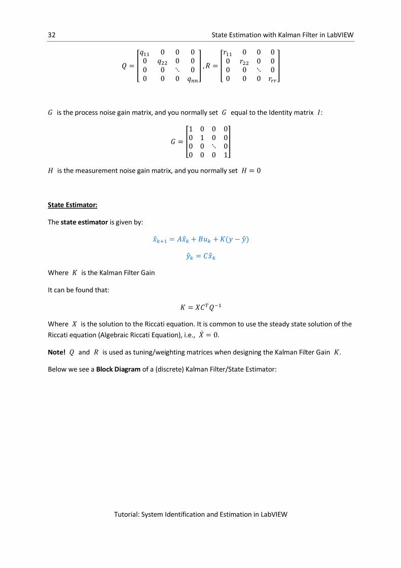
It is normal to let and be diagonal matrices:
32 State Estimation with Kalman Filter in LabVIEW
Tutorial: System Identification and Estimation in LabVIEW
[
] [
]
is the process noise gain matrix, and you normally set equal to the Identity matrix :
[
]
is the measurement noise gain matrix, and you normally set
State Estimator:
The state estimator is given by:
( )
Where is the Kalman Filter Gain
It can be found that:
Where is the solution to the Riccati equation. It is common to use the steady state solution of the
Riccati equation (Algebraic Riccati Equation), i.e., .
Note! and is used as tuning/weighting matrices when designing the Kalman Filter Gain .
Below we see a Block Diagram of a (discrete) Kalman Filter/State Estimator:

33 State Estimation with Kalman Filter in LabVIEW
Tutorial: System Identification and Estimation in LabVIEW
LabVIEW:
In LabVIEW Design and Simulation Module we use the “CD Kalman Gain.vi” in order to find K:
LabVIEW Functions Palette: Control Design & Simulation → Control Design → State Feedback Design
→ CD Kalman Gain.vi
Note! In LabVIEW is used as a symbol for the Kalman Filter Gain matrix.
Note! The “Kalman Filter Gain.vi” is polymorphic, depending on what kind of model
(deterministic/stochastic or continuous/discrete) you wire to this VI, the inputs changes
automatically or you may use the polymorphic selector below the VI:

34 State Estimation with Kalman Filter in LabVIEW
Tutorial: System Identification and Estimation in LabVIEW
Deterministic and Continuous:
Stochastic and Continuous:
Deterministic and Discrete:
Stochastic and Discrete:
LabVIEW Example: Find the Kalman Gain
Block Diagram:
Front Panel:

35 State Estimation with Kalman Filter in LabVIEW
Tutorial: System Identification and Estimation in LabVIEW
[End of Example]
MathScript:
Use the functions kalman, kalman_d or lqe to find the Kalman gain matrix.
Function Description Example
kalman Calculates the optimal steady-state Kalman gain K
that minimizes the covariance of the state
estimation error. You can use this function to
calculate K for continuous and discrete system
models.
>>[SysKal, K]=kalman(ssmodel, Q, R)
kalman_d Calculates the optimal steady-state Kalman gain K
that minimizes the covariance of the state
estimation error. The input system and noise
covariance are based on a continuous system. All
outputs are based on a discretized system, which
is based on the sample rate Ts.
[SysKalDisc, K]=kalman_d(ssmodel, Q,
R, Ts)
lqe Calculates the optimal steady-state estimator
gain matrix K for a continuous state-space model
defined by matrices A and C.
K=lqe(A,G,C,Q,R)
MathScript Example: Find Kalman Gain using the Kalman function
MathScript Code for finding the steady state Kalman Gain:
% Define the State-space model:
c=1;

36 State Estimation with Kalman Filter in LabVIEW
Tutorial: System Identification and Estimation in LabVIEW
m=1;
k=1;
A = [0 1; -k/m -c/m];
B = [0; 1/m];
C = [1 0];
ssmodel = ss(A, B, C);
% Discrete model:
Ts=0.1; % Sampling Time
discretemodel = c_to_d(ssmodel, Ts);
% Check for Observability:
O = obsvmx(discretemodel);
r = rank(O);
% Find Kalman Gain
Q=[0.01 0; 0 0.01];
R=[0.01];
[SysKal, K]=kalman(discretemodel, Q, R);
K
The Output is:
K =
0.64435
0.10759
[End of Example]
MathScript Example: Find Kalman Gain using the Kalman function
MathScript Code for finding the steady state Kalman Gain:
% Define the State-space model:
c=1;
m=1;
k=1;
A = [0 1; -k/m -c/m];
B = [0; 1/m];
G=[1 0 ; 0 1];
C = [1 0];
% Find Kalman Gain
Q=[0.01 0; 0 0.01];
R=[0.01];
K=lqe(A,G,C,Q,R)
The Output is:
K =
0.86121
-0.12916
[End of Example]

37 State Estimation with Kalman Filter in LabVIEW
Tutorial: System Identification and Estimation in LabVIEW
5.4 State Estimation
LabVIEW Control Design and Simulation Module have built-in functionality for State Estimation using
the Kalman Filter.
In the next section we will create our own Kalman Filter State Estimation algorithm.
LabVIEW:
There are different functions and VIs for finding the State Estimation using the Kalman Filter.
CD State Estimator.vi:
LabVIEW Functions Palette: Control Design & Simulation → Control Design → State Feedback Design
→ CD State Estimator.vi
Below we show an example of how to use the CD State Estimator.vi in LabVIEW.
LabVIEW Example: State Estimator Simulation
Given the following model:
[ ] 0
1⏟
0 1 0
1
⏟
, -⏟
0 1 , -⏟
We will use the “CD State Estimator.vi” in LabVIEW.
Block Diagram becomes as follows:

38 State Estimation with Kalman Filter in LabVIEW
Tutorial: System Identification and Estimation in LabVIEW
Note! We have used “CD Initial Response.vi” for plotting the response. The VI is located in the
LabVIEW Functions Palette: Control Design & Simulation → Control Design → Time Response → CD
Initial Response.vi
The result becomes as follows:
We see the estimates are good.
MathScript:
In MathScript we may use the built-in estimator function.
5.5 LabVIEW Kalman Filter Implementations
LabVIEW Design and Simulation Module have several built-in versions of the Kalman Filter; here we
will investigate some of them.
The Control Design → Implementation palette in LabVIEW:

39 State Estimation with Kalman Filter in LabVIEW
Tutorial: System Identification and Estimation in LabVIEW
Here we have the “CD Discrete Kalman Filter”.
Simulation → Estimation palette in LabVIEW:
Here we have implementations for:
Continuous Kalman Filter
Continuous Extended Kalman Filter
Discrete Kalman Filter
Discrete Extended Kalman Filter
We will go through the “Discrete Kalman Filter” in detail and show some examples.
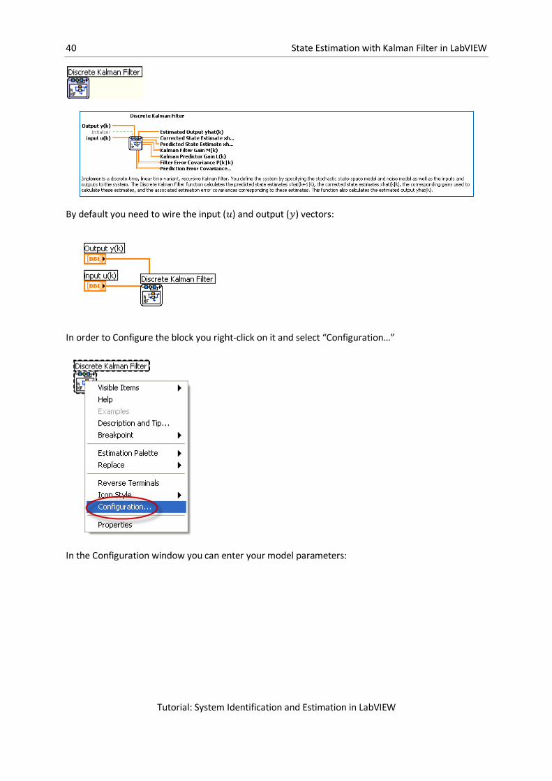
Discrete Kalman Filter:
LabVIEW Functions Palette: Control Design & Simulation → Simulation → Estimation → Discrete
Kalman Filter
40 State Estimation with Kalman Filter in LabVIEW
Tutorial: System Identification and Estimation in LabVIEW
By default you need to wire the input ( ) and output ( ) vectors:
In order to Configure the block you right-click on it and select “Configuration…”
In the Configuration window you can enter your model parameters:
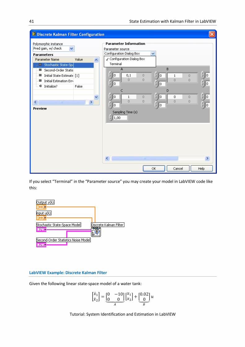
41 State Estimation with Kalman Filter in LabVIEW
Tutorial: System Identification and Estimation in LabVIEW
If you select “Terminal” in the “Parameter source” you may create your model in LabVIEW code like
this:
LabVIEW Example: Discrete Kalman Filter
Given the following linear state-space model of a water tank:
[ ] 0
1⏟
0 1 0
1
⏟

42 State Estimation with Kalman Filter in LabVIEW
Tutorial: System Identification and Estimation in LabVIEW
, -⏟
0 1 , -⏟
Where is the level in the tank, while is the outflow of the tank. Only the level is
measured.
Step 1: First we create the model:
Where A, B, D and D is defined according to the state-space model above:
Note! The Discrete Kalman Filter function in LabVIEW requires a stochastic state-space model, so we
have to create a stochastic state-space model or convert our state-space model into a stochastic
state-space model as done in the LabVIEW code above.
Step 2: Then we use the Discrete Kalman Filter function in LabVIEW on our model:

43 State Estimation with Kalman Filter in LabVIEW
Tutorial: System Identification and Estimation in LabVIEW
The Discrete Kalman Filter function also requires a Noise model, so we create a noise model from our
and matrices as done in the LabVIEW code above.
The results are as follows:
We see the result is very good.
[End of Example]

44
6 Create your own Kalman Filter
from Scratch
In this chapter we will create our own Kalman Filter Algorithm from scratch.
6.1 The Kalman Filter Algorithm
LabVIEW Design and Simulation Module have several built-in versions of the Kalman Filter, but in this
chapter we will create our own Kalman Filter algorithm.
Here is a step by step Kalman Filter algorithm which can be directly implemented in a programming
language, such as LabVIEW. You may, e.g., implement it in standard LabVIEW code or a Formula
Node in LabVIEW.
Pre Step: Find the steady state Kalman Gain K
K is time-varying, but you normally implement the steady state version of Kalman Gain K. Use the
“CD Kalman Gain.vi” in LabVIEW or one of the functions kalman, kalman_d or lqe in MathScript.
Init Step: Set the initial Apriori (Predicted) state estimate
Step 1: Find Measurement model update
( )
For Linear State-space model:
Step 2: Find the Estimator Error
Step 3: Find the Aposteriori (Corrected) state estimate
Where K is the Kalman Filter Gain. Use the steady state Kalman Gain or calculate the time-varying
Kalman Gain.
Step 4: Find the Apriori (Predicted) state estimate update
( )

45 Create your own Kalman Filter from Scratch
Tutorial: System Identification and Estimation in LabVIEW
For Linear State-space model:
Step 1-4 goes inside a loop in your program.
This is the algorithm we will implement in the example below.
6.2 Examples
LabVIEW Example: Kalman Filter algorithm
Given the following linear state-space model of a water tank:
[ ] 0
1⏟
0 1 0
1
⏟
, -⏟
0 1 , -⏟
Where is the level in the tank, while is the outflow of the tank. Only the level is
measured.
First we have to find the steady state Kalman Filter Gain and check for Observability:
Then we run the real process (or simulated model) in parallel with the Kalman Filter in order to find
estimates for and :

46 Create your own Kalman Filter from Scratch
Tutorial: System Identification and Estimation in LabVIEW
In this case we have used a Simulation Loop, but a While Loop will do the same.
Blocks/SubVIs:
Real process/Simulated process:
Here we either have a model of the system or read/write data from the real process using a
DAQ card, e.g., USB-6008 from National Instruments.
Implementation of the Kalman Filter Algorithm:
The Block Diagram is as follows:

47 Create your own Kalman Filter from Scratch
Tutorial: System Identification and Estimation in LabVIEW
This is a general implementation and will work for all linear discrete systems.
The results are as follows:

48 Create your own Kalman Filter from Scratch
Tutorial: System Identification and Estimation in LabVIEW
[End of Example]

49
7 Overview of Kalman Filter
functions in LabVIEW
In LabVIEW there are several VIs and functions used for Kalman Filter implementations.
7.1 Control Design palette
In the “Control Design” palette we find subpalettes for “State Feedback Design” and
“Implementation”:
7.1.1 State Feedback Design subpalette
In the “State Feedback Design” subpalette we find VIs for calculation the Kalman Gain, etc.

50 Overview of Kalman Filter functions in LabVIEW
Tutorial: System Identification and Estimation in LabVIEW
→ Use the State Feedback Design VIs to calculate controller and observer gains for closed-loop state
feedback control or to estimate a state-space model. You also can use State Feedback Design VIs to
configure and test state-space controllers and state estimators in time domains.
Kalman Filter Gain VI:
7.1.2 Implementation subpalette
In the “Implementation” subpalette we find VIs for implementing a discrete Observer and a discrete
Kalman Filter.
→ Use the Implementation VIs and functions to simulate the dynamic response of a discrete system
model, deploy a discrete model to a real-time target, implement a discrete Kalman filter, and
implement current and predictive observers.
Discrete Kalman Filter:

51 Overview of Kalman Filter functions in LabVIEW
Tutorial: System Identification and Estimation in LabVIEW
7.2 Simulation palette
In the “Simulation” palette we find the “Estimation“ subpalette:
7.2.1 Estimation subpalette
In the “Estimation” palette we find VIs for implementing a continuous/discrete Kalman Filter.

52 Overview of Kalman Filter functions in LabVIEW
Tutorial: System Identification and Estimation in LabVIEW
→ Use the Estimation functions to estimate the states of a state-space system. The state-space
system can be deterministic or stochastic, continuous or discrete, linear or nonlinear, and completely
or partially observable.
Continuous Kalman Filter VIs:

53 Overview of Kalman Filter functions in LabVIEW
Tutorial: System Identification and Estimation in LabVIEW
Discrete Kalman Filter VIs:

54
8 State Estimation with Observers
in LabVIEW
Observers are an alternative to the Kalman Filter. An Observer is an algorithm for estimating the
state variables in a system based on a model of the system. Observers have the same structure as a
Kalman Filter.
In Observers you specify how fast and stable you want the estimates to converge to the real values,
i.e., you specify the eigenvalues of the system. Based on the eigenvalues you will find the Observer
gain K that is used to update the estimates.
One simple way to find the eigenvalues is to use the Butterworth eigenvalues from the Butterworth
polynomial. When we have found the eigenvalues we can then use the Ackerman in order to find the
Observer gain.
LabVIEW Control Design and Simulation Module have lots of functionality for State Estimation using
Observers. The functionality will be explained in detail in the next chapters.
8.1 State-Space model
Given the continuous linear state space-model:
Or given the discrete linear state space-model

55 State Estimation with Observers in LabVIEW
Tutorial: System Identification and Estimation in LabVIEW
LabVIEW:
In LabVIEW we may use the “CD Construct State-Space Model.vi” to create a State-space model:
Note! If you specify a discrete State-space model you have to specify the Sampling Time.
LabVIEW Example: Create a State-space model
Block Diagram:
The matrices , , and may be defined on the Front Panel like this:
[End of Example]

56 State Estimation with Observers in LabVIEW
Tutorial: System Identification and Estimation in LabVIEW
8.2 Eigenvalues
One simple way to find the eigenvalues is to use the Butterworth eigenvalues from the Butterworth
polynomial.
Butterwort Polynomial:
The Butterworth Polynomial is defined as:
( )
where are the coefficients in the Butterworth Polynomial.
Here we will use a 2.order Butterworth Polynomial, which is defined as:
( )
where √ .
This gives:
( ) √
where the parameter is used to defined the speed of the response according to:
where is defined as the Observer response time where the step response reach 63% of the
steady state value of the response.
→ So we will use as the tuning parameter for the Observer.
LabVIEW:
In LabVIEW we can use the “Polynomial Roots.vi” to find the roots based on the Butterworth
Polynomial
LabVIEW Functions Palette: Mathematics → Polynomial → Polynomial Roots.vi

57 State Estimation with Observers in LabVIEW
Tutorial: System Identification and Estimation in LabVIEW
Below we see the Mathematics and the Polynomial palettes in LabVIEW.
MathScript:
In MathScript we can use the roots function in order to find the eigenvalues based on a given
polynomial.
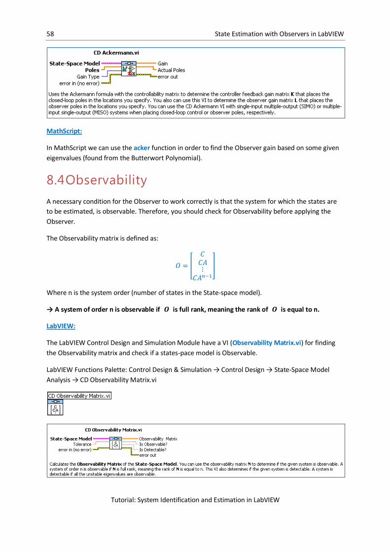
8.3 Observer Gain
LabVIEW:
In LabVIEW we can use the “CD Ackerman.vi” to find the Observer gain based on some given
eigenvalues (found from the Butterwort Polynomial).
LabVIEW Functions Palette: Control Design & Simulation → Control Design → State Feedback Design
→ CD Ackerman.vi
58 State Estimation with Observers in LabVIEW
Tutorial: System Identification and Estimation in LabVIEW
MathScript:
In MathScript we can use the acker function in order to find the Observer gain based on some given
eigenvalues (found from the Butterwort Polynomial).
8.4 Observability
A necessary condition for the Observer to work correctly is that the system for which the states are
to be estimated, is observable. Therefore, you should check for Observability before applying the
Observer.
The Observability matrix is defined as:
[
]
Where n is the system order (number of states in the State-space model).
→ A system of order n is observable if is full rank, meaning the rank of is equal to n.
LabVIEW:
The LabVIEW Control Design and Simulation Module have a VI (Observability Matrix.vi) for finding
the Observability matrix and check if a states-pace model is Observable.
LabVIEW Functions Palette: Control Design & Simulation → Control Design → State-Space Model
Analysis → CD Observability Matrix.vi

59 State Estimation with Observers in LabVIEW
Tutorial: System Identification and Estimation in LabVIEW
Note! In LabVIEW is used as a symbol for the Observability matrix.
LabVIEW Example: Check for Observability
[End of Example]
MathScript:
In MathScript you may use the obsvmx function to find the Observability matrix. You may then use
the rank function in order to find the rank of the Observability matrix.
MathScript Example:
The following MathScript Code check for Observability:
% Check for Observability:
O = obsvmx (discretemodel)
r = rank(O)
[End of Example]
8.5 Examples
Here we will show implementations of an Observer in LabVIEW and MathScript.
Given the following linear state-space model of a water tank:
[ ] 0
1⏟
0 1 0
1
⏟
, -⏟
0 1 , -⏟
Where is the level in the tank, while is the outflow of the tank. Only the level is
measured.

60 State Estimation with Observers in LabVIEW
Tutorial: System Identification and Estimation in LabVIEW
LabVIEW Example: Observer Gain
Below we see the Block Diagram in LabVIEW for calculating the Observer gain:
We used the “Polynomial Roots.vi” in order to find the poles as specified in the Butterworth
Polynomial.
We use a 2.order Butterworth Polynomial:
( ) √
where the parameter is used to defined the speed of the response according to:
In the example we set and in the example.
This gives:
( )
So the coefficients in the polynomial are as follows:
Then we have used the “CD Akerman.vi” to find the Observer gain.
The result becomes:
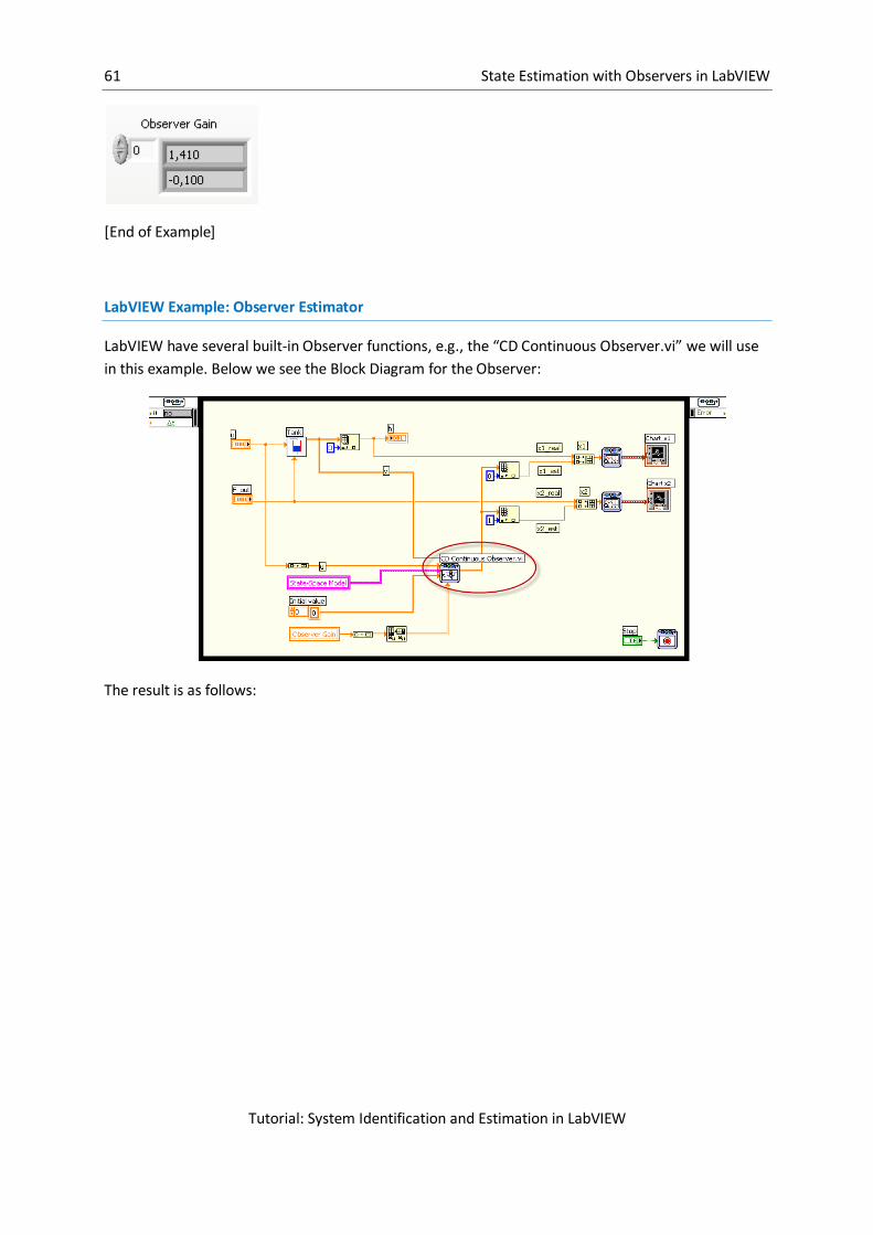
61 State Estimation with Observers in LabVIEW
Tutorial: System Identification and Estimation in LabVIEW
[End of Example]
LabVIEW Example: Observer Estimator
LabVIEW have several built-in Observer functions, e.g., the “CD Continuous Observer.vi” we will use
in this example. Below we see the Block Diagram for the Observer:
The result is as follows:

62 State Estimation with Observers in LabVIEW
Tutorial: System Identification and Estimation in LabVIEW
[End of Example]
MathScript Example: Observer Gain
Here we will use MathScript in order to find the Observer gain for the same system as above.
The Code is as follows:
% Define the State-space model:
A = [0 -10; 0 0];
B = [0.02; 0];
C = [1 0];
D=[0];
ssmodel = ss(A, B, C,D);
% Check for Observability:
O = obsvmx (ssmodel);
r = rank(O);
%Butterwort Polynomial:
B2=[1, 1.41, 1];
p=roots(B2);
% Find Observer Gain
K = ackermann(ssmodel, p, 'L')
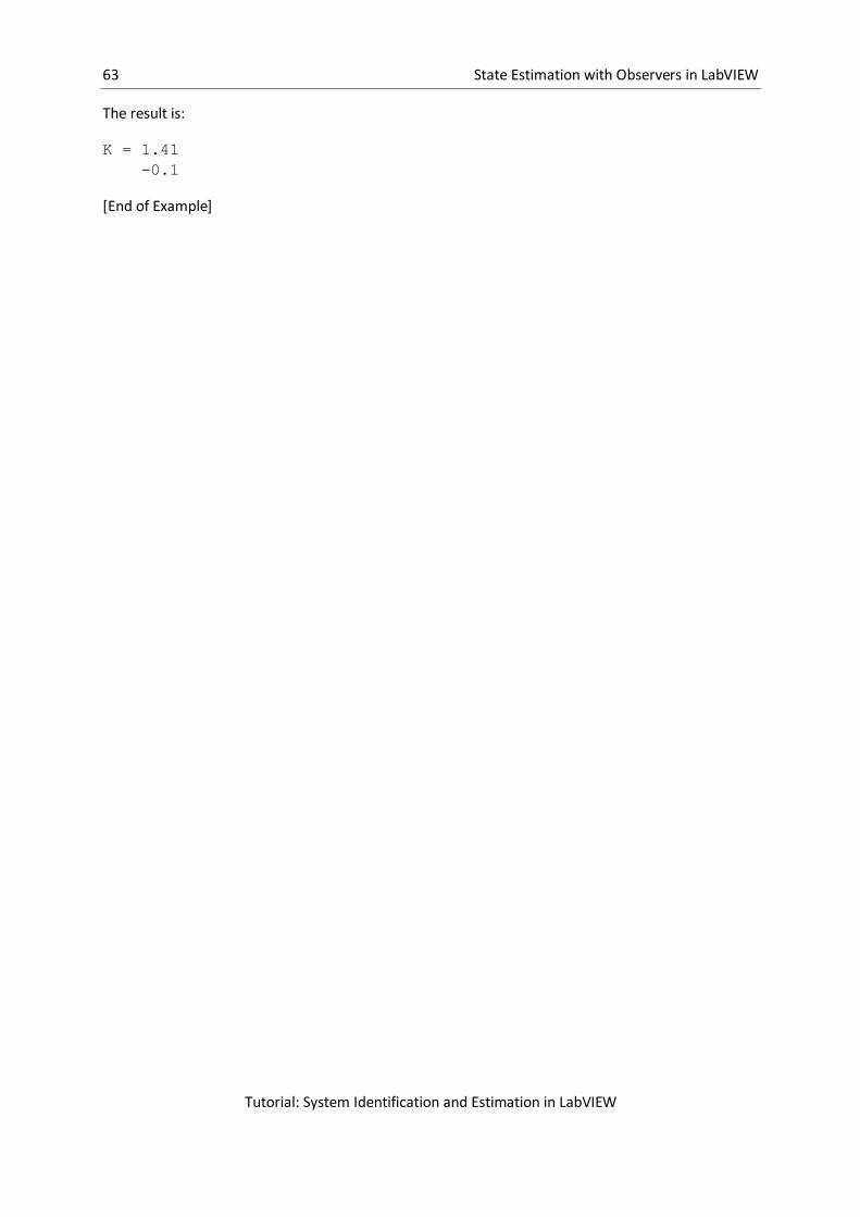
63 State Estimation with Observers in LabVIEW
Tutorial: System Identification and Estimation in LabVIEW
The result is:
K = 1.41
-0.1
[End of Example]

64
9 Overview of Observer functions
Observers are very similar to Kalman filters. In observers the estimator gain is calculated from
specified eigenvalues or poles of the estimator error dynamics (in other words: how fast you want
the estimation error to converge to real states).
In LabVIEW there are several VIs and functions used for Observer implementations.
9.1 Control Design palette
In the “Control Design” palette we find subpalettes for “State Feedback Design” and
“Implementation”:
9.1.1 State Feedback Design subpalette
In the “State Feedback Design” subpalette we find VIs for calculation the Observer Gain, etc.

65 Overview of Observer functions
Tutorial: System Identification and Estimation in LabVIEW
→ Use the State Feedback Design VIs to calculate controller and observer gains for closed-loop state
feedback control or to estimate a state-space model. You also can use State Feedback Design VIs to
configure and test state-space controllers and state estimators in time domains.
Ackermann VI:
9.1.2 Implementation subpalette
In the “Implementation” subpalette we find VIs for implementing a discrete Observer and a discrete
Kalman Filter.
→ Use the Implementation VIs and functions to simulate the dynamic response of a discrete system
model, deploy a discrete model to a real-time target, implement a discrete Kalman filter, and
implement current and predictive observers.

66 Overview of Observer functions
Tutorial: System Identification and Estimation in LabVIEW
Discrete Observer:
9.2 Simulation palette
In the “Simulation” palette we find the “Estimation“ subpalette:
9.2.1 Estimation subpalette
In the “Estimation” palette we find VIs for implementing continuous/discrete Observers and Kalman
Filter.
67 Overview of Observer functions
Tutorial: System Identification and Estimation in LabVIEW
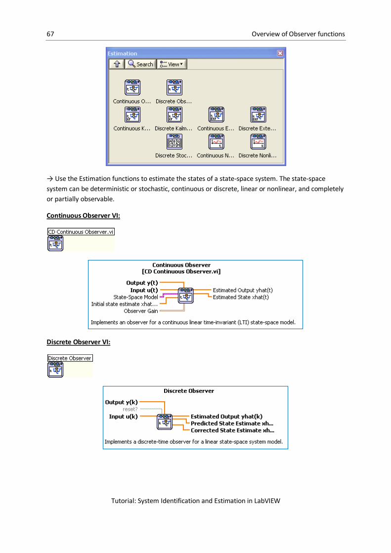
→ Use the Estimation functions to estimate the states of a state-space system. The state-space
system can be deterministic or stochastic, continuous or discrete, linear or nonlinear, and completely
or partially observable.
Continuous Observer VI:
Discrete Observer VI:
68
Part III: System Identification

69
10 System Identification in
LabVIEW
The model can be in form of differential equations developed from physical principles or from
transfer function models, which can be regarded as “black-box”-models which expresses the
input-output property of the system. Some of the parameters of the model can have unknown or
uncertain values, for example a heat transfer coefficient in a thermal process or the time-constant in
a transfer function model. We can try to estimate such parameters from measurements taken during
experiments on the system.
Here we will discuss:
Parameter Estimation and the Least Square Method (LS)
Sub-space methods/Black-Box methods
Polynomial Model Estimation: ARX/ARMAX model Estimation
In LabVIEW we can use the “System Identification Toolkit”.
The “System Identification” palette in LabVIEW:

70 System Identification in LabVIEW
Tutorial: System Identification and Estimation in LabVIEW
In the next chapters we will use the different functionality available in the System Identification
Toolkit.
10.1 Parameter Estimation with Least Square
Method (LS)
Parameter Estimation using the Least Square Method (LS) is used to find a model with unknown
physical parameters in a mathematical model.
The Least square method can be written as:
Where
is the unknown parameter vector
is the known measurement vector
is the known regression matrix
The solution for may be found as:
It can be found that the least square solution for is:
( )
Implementation in MathScript/MATLAB:
theta=inv(phi’*phi)* phi’*Y
or simply:
theta=phi\Y
In LabVIEW we can use the blocks (“AxB.vi”, “Transpose Matrix.vi”, “Inverse Matrix.vi”) in the “Linear
Algebra” (located in the Mathematics palette) palette in order to fin the Least Square solution:

71 System Identification in LabVIEW
Tutorial: System Identification and Estimation in LabVIEW
We can also use the “Solve Linear Equations.vi”:
Example:
Given the following model:
( )
The following values are found from experiments:
( )
( )
( )
We will find the unknowns and using the Least Square (LS) method in MathScript/LabVIEW.
We have that:
Where
is the unknown parameter vector
is the known measurement vector
is the known regression matrix

72 System Identification in LabVIEW
Tutorial: System Identification and Estimation in LabVIEW
The solution for may be found as (if is a quadratic matrix):
It can be found that the least square solution for is:
( )
We get:
This becomes:
[ ]
⏟
[
]⏟
0 1⏟
MathScript:
We define and in MathScript and find by:
phi = [1 1; 2 1; 3 1];
Y = [0.8 3.0 4.0]';
theta = inv(phi'*phi)* phi'*Y
%or simply by
theta=phi\Y
The answer becomes:
theta = 1.6
-0.6
i.e.:
This gives:
( )

73 System Identification in LabVIEW
Tutorial: System Identification and Estimation in LabVIEW
LabVIEW:
Block Diagram:
Front Panel:
We can also use the “Solve Linear Equations.vi” directly:
[End of Example]
10.2 System Identification using Sub-space
methods/Black-Box methods
Sub-space methods/Black-Box methods is used to find a model with non-physical parameters.
A sub-space methods/Black-Box method estimates a linear discrete State-space model on the form:

74 System Identification in LabVIEW
Tutorial: System Identification and Estimation in LabVIEW
LabVIEW offers functionality for this. In the “Parametric Model Estimation” palette we find the “SI
Estimate State-Space Model.vi” which can be used for sub-space identification.
“Parametric Model Estimation” palette:
This VI estimates the parameters of a state-space model for an unknown system.
10.3 System Identification using Polynomial
Model Estimation: ARX/ARMAX model
Estimation
LabVIEW offers VIs for ARX/ARMAX model estimation in the “Parametric Model Estimation” palette.

75 System Identification in LabVIEW
Tutorial: System Identification and Estimation in LabVIEW
For ARX models we can use “SI Estimate ARX model”:
For ARMAX models we can use “SI Estimate ARMAX model”:
10.4 Generate model Data
In order to find a model we need to generate data based on the real process. The stimulus (exitation)
signal and the response signal will then be input to the functions/VIs (algorithms) in LabVIEW that
you will use to model your process.
Below we explain how we do this in LabVIEW.

76 System Identification in LabVIEW
Tutorial: System Identification and Estimation in LabVIEW
Datalogging:
Use LabVIEW for exciting the process and logging signals. Use open-loop experiments (no feedback
control system). You can use the Write to Measurement File function on the File I/O palette in
LabVIEW for writing data to text files (use the LVM data file format, not the TDMS file format which
give binary files).
In the File I/O palette in LabVIEW we have lots of functionality for writing and reading files.
Below we see the “File I/O” palette in LabVIEW:
In this Tutorial we will focus on the “Write To Measurement File” and “Read From Measurement
File”.
The “Write To Measurement File” and “Read From Measurement File” is so-called “Express VIs”.
When you drag these VI’s to the Block Diagram, a configuration dialog pops-up immediately, like this:

77 System Identification in LabVIEW
Tutorial: System Identification and Estimation in LabVIEW
In this configuration dialog you set file name, file type, etc.
Note that these “Express VIs” have no Block Diagram.
10.4.1 Excitation signals
It is important to have a good excitation signal, you can use different excitation signals, such as:
A PRBS signal (Pseudo Random Binary Signal)
A Chirp Signal
A Up-down signal
LabVIEW:
In LabVIEW you can use some of the functions in the Signal Generation palette:

78 System Identification in LabVIEW
Tutorial: System Identification and Estimation in LabVIEW
LabVIEW Functions Palette: Signal Processing → Signal Generation
PRBS Signal A PRBS signal looks like this:
LabVIEW:
In LabVIEW you can use the “SI Generate Pseudo-Random Binary Sequence.vi” function.
LabVIEW Functions Palette: Control Design & Simulation → System identification → Utilities → SI
Generate Pseudo-Random Binary Sequence.vi
79 System Identification in LabVIEW
Tutorial: System Identification and Estimation in LabVIEW
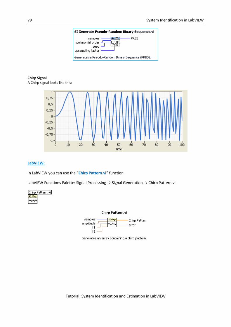
Chirp Signal A Chirp signal looks like this:
LabVIEW:
In LabVIEW you can use the “Chirp Pattern.vi” function.
LabVIEW Functions Palette: Signal Processing → Signal Generation → Chirp Pattern.vi

80
11 Overview of System
Identification functions
In LabVIEW we can use the System Identification Toolkit.
The “System Identification” palette in LabVIEW:
→ Use the System Identification VIs to create and estimate mathematical models of dynamic
systems. You can use the VIs to estimate accurate models of systems based on observed
input-output data.
The “System Identification” palette in LabVIEW has the following subpalettes:
Icon Name Description
Preprocessing
Data Preprocessing
Use the Data Preprocessing VIs to preprocess
the raw data that you acquired from an
unknown system.
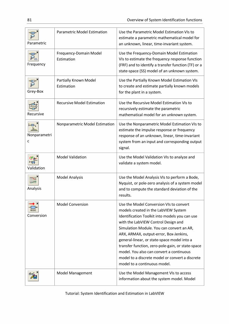
81 Overview of System Identification functions
Tutorial: System Identification and Estimation in LabVIEW
Parametric
Parametric Model Estimation
Use the Parametric Model Estimation VIs to
estimate a parametric mathematical model for
an unknown, linear, time-invariant system.
Frequency
Frequency-Domain Model
Estimation
Use the Frequency-Domain Model Estimation
VIs to estimate the frequency response function
(FRF) and to identify a transfer function (TF) or a
state-space (SS) model of an unknown system.
Grey-Box
Partially Known Model
Estimation
Use the Partially Known Model Estimation VIs
to create and estimate partially known models
for the plant in a system.
Recursive
Recursive Model Estimation
Use the Recursive Model Estimation VIs to
recursively estimate the parametric
mathematical model for an unknown system.
Nonparametri
c
Nonparametric Model Estimation
Use the Nonparametric Model Estimation VIs to
estimate the impulse response or frequency
response of an unknown, linear, time-invariant
system from an input and corresponding output
signal.
Validation
Model Validation
Use the Model Validation VIs to analyze and
validate a system model.
Analysis
Model Analysis
Use the Model Analysis VIs to perform a Bode,
Nyquist, or pole-zero analysis of a system model
and to compute the standard deviation of the
results.
Conversion
Model Conversion
Use the Model Conversion VIs to convert
models created in the LabVIEW System
Identification Toolkit into models you can use
with the LabVIEW Control Design and
Simulation Module. You can convert an AR,
ARX, ARMAX, output-error, Box-Jenkins,
general-linear, or state-space model into a
transfer function, zero-pole-gain, or state-space
model. You also can convert a continuous
model to a discrete model or convert a discrete
model to a continuous model.
Model Management
Use the Model Management VIs to access
information about the system model. Model

82 Overview of System Identification functions
Tutorial: System Identification and Estimation in LabVIEW
Management information includes properties such as the
system type, sampling rate, system dimensions,
noise covariance, and so on.
Utilities
Utilities
Use the Utilities VIs to perform miscellaneous
tasks on data or the system model, including
producing data samples, displaying model
equations, merging models, and so on.
The “Data Preprocessing” palette in LabVIEW:
Some important functions in the “Data Preprocessing” palette are:
The “Parametric Model Estimation” palette in LabVIEW:

83 Overview of System Identification functions
Tutorial: System Identification and Estimation in LabVIEW
Some important functions in the “Parametric Model Estimation” palette are:
The “Parametric Model Estimation” palette in LabVIEW has subpalette for “Polynomial Model
Estimation”:

84 Overview of System Identification functions
Tutorial: System Identification and Estimation in LabVIEW
→ Use the Polynomial Model Estimation VIs to estimate an AR, ARX,ARMAX, Box-Jenkins, or
output-error model for an unknown, linear, time-invariant system.
Some important functions in the “Polynomial Model Estimation” palette are:

85
12 System Identification Example
We want to identify the model of a given system.
We have found the model to be:
( )
where
is the time constant
is the system gain, e.g. pump gain
is the time-delay
→ We want to find the model parameters using the Least Square method. We will use
LabVIEW and MathScript.
Set the system on the form
Solutions:
We get:
⏟
, ( )-⏟
[
]
⏟
i.e.
[
]
In order to find using the Least Square method we need to log input and output data. This means
we need to discretize the system.
We use a simple Euler forward method:
is the sampling time.

86 System Identification Example
Tutorial: System Identification and Estimation in LabVIEW
This gives:
⏟
[
]⏟
[
]
⏟
Let’s assume (which can be found from a simple step response on the real system), we then
get (with sampling time ):
⏟
, -⏟
[
]
⏟
Note! In 3 seconds we log 30 points with data using sampling time !!!
Given the following logging data (the data is just for illustration and not realistic):
1 0.9 3
2 1.0 4
3 1.1 5
4 1.2 6
5 1.3 7
6 1.4 8
7 1.5 9
We use the following sampling time:
From a simple step response we have found the time-delay to be: .
→ Set the system on the form
Solutions:
With time-delay and we get:
⏟
, -⏟
[
]
⏟

87 System Identification Example
Tutorial: System Identification and Estimation in LabVIEW
Using the given data set we can set on the form :
[
] [
] [
]
i.e.:
[ ]
⏟
[
]⏟
[
]
⏟
Note! We need to make sure the dimensions are correct.
→ We find the model parameters ( ) using MathScript
MathScript gives:
clear, clc
Y = [1, 1, 1]';
phi = [6, 0.9; 7, 1.0; 8, 1.1];
theta = phi\Y
%or
theta = inv(phi'*phi)*phi'*Y
T = -1/theta(1)
K = theta(2)
MathScript responds with the following answers:
theta =
-0.3333
3.3333
T =
3
K =
3.3333
i.e., the model parameters become:

88 System Identification Example
Tutorial: System Identification and Estimation in LabVIEW
Which gives the following modell:
( )
With values:
( )
Implement the model in LabVIEW. Use , , and
simulate the system. Plot the step response for the system.
Model:
( )
Where , ,
Solutions:
We implement the model using a “Simulation Subsystem” and use the available blocks in the Control
and Design Module.
The model may be implemented as follows:
We simulate the system using the following program:
Block Diagram:

89 System Identification Example
Tutorial: System Identification and Estimation in LabVIEW
Front Panel:
We do a simple step response:

90 System Identification Example
Tutorial: System Identification and Estimation in LabVIEW
Find the transfer function for the system:
( ) ( )
( )
Model:
( )
Plot the step response for the transfer function in MathScript. Compare and discuss the results from
previous task.
Solutions:
We use the differential equation:
( )
Laplace transformation gives:
( )
( ) ( )
Note! We use the following Laplace transformation:
( ) ( )
( ) ( )
Then we get:
( )
( ) ( )
and:
( )(
) ( )
and:
( )
( )
Finally:

91 System Identification Example
Tutorial: System Identification and Estimation in LabVIEW
( ) ( )
( )
With values ( , , ):
( ) ( )
( )
MathScript:
We implement the transfer function in MathScript and perform a step response. We use the step()
function.
clear, clc
s=tf('s');
K=2;
T=5;
H1=tf(K*T/(T*s+1));
delay=3;
H2=set(H1,'inputdelay',delay);
step(H2)
% You may also use:
figure(2)
H = sys_order1(K*T, T, delay)
step(H)
The step response becomes:

92 System Identification Example
Tutorial: System Identification and Estimation in LabVIEW
→ We see that the step response is the same as in the previous task.
Log input and output data based on the model.
Model:
( )
Where , ,
Solutions:
We save the data using “Write To Measurement File” in LabVIEW.
Based on a simple step response we can find the time-delay .
We use the same application as in a previous task:

93 System Identification Example
Tutorial: System Identification and Estimation in LabVIEW
Find the model parameters ( og ) using Least Square in LabVIEW based on the logged
data.
Note! The answers should be and .
Model:
( )
Where , ,
Solutions:
It is a good idea to split your program into different logical parts using, e.g., SubVIs in LabVIEW.
The different parts/steps could, e.g., be:
1. Get Logged Data from File
a. Input: File Name
b. Outputs: and ( )
2. Transform the data and stack data into and
a. Inputs: and ( )

94 System Identification Example
Tutorial: System Identification and Estimation in LabVIEW
b. Outputs: and
3. Find the Least Square solution ( )
a. Input: and
b. Output: ( )
LabVIEW code:
Block Diagram:
Front Panel:

95 System Identification Example
Tutorial: System Identification and Estimation in LabVIEW
→ As you see the result is and (as expected).
The different SubVI’s do the following:
1. “Open Measurement Data from File.vi”
This SubVI opens the logged data from file (created in a previous task).
Block Diagram:

96 System Identification Example
Tutorial: System Identification and Estimation in LabVIEW
2. “Create LS Matrices from Logged Data with Time Delay.vi”
This SubVI “stack” data on the form:
⏟
[
]⏟
[
]
⏟
Block Diagram:
3. “Find LS Solution.vi”
This SubVI find the LS solution:
( )
Block Diagram:

97 System Identification Example
Tutorial: System Identification and Estimation in LabVIEW

Telemark University College
Faculty of Technology
Kjølnes Ring 56
N-3914 Porsgrunn, Norway
www.hit.no
Hans-Petter Halvorsen, M.Sc.
Telemark University College
Department of Electrical Engineering, Information Technology and Cybernetics
Phone: +47 3557 5158
E-mail: [email protected]
Blog: http://home.hit.no/~hansha/
Room: B-237a