system identification and control of an arleigh burke
TRANSCRIPT


DUDLEY KNOX LIBRARYOSTGRADUATF SCHOOLREY CA 93943-5101


System Identification and Control of an Arleigh Burke Class
Destroyer Using an Extended Kalman Filter
by
Michael Eric Taylor
B.S., Civil Engineering
University of South Carolina, 1993
Submitted to the Departments of Ocean Engineering and Mechanical Engineering
in partial fulfillment of the requirements for the degrees of
Naval Engineer
and
Master of Science in Mechanical Engineering
at the
MASSACHUSETTS INSTITUTE OF TECHNOLOGYJune 2000
©2000 Michael E. Taylor. All rights reserved.
The author hereby grants to MIT permission to reproduce
and to distribute publicly paper and electronic
copies of this thesis document in whole or in part.

DUDLEY KNOX LIBRARYNAVAL POSTGRADUATE SCHOOLMONTEREY ~A S3943-5101
MS fVvoWtue

System Identification and Control of an Arleigh Burke Class Destroyer
Using an Extended Kalman Filter
by
Michael Eric Taylor
Submitted to the Departments of Ocean Engineering and Mechanical Engineering
on May 15. 2000. in partial fulfillment of the
requirements for the degrees of
Naval Engineer
and
Master of Science in Mechanical Engineering
Abstract
Maneuvering characteristics of surface combatants in the United States Navy are often
ignored during the design process. Key maneuvering parameters such as tactical diameter
and turning rate are determined during sea trials after the ship enters service. In the "Navy
After Next", the study of maneuvering of surface combatants will become increasingly more
important in efforts to reduce the number of personnel required to operate the ship and
rims reduce life cycle costs. This thesis attempts to address this issue.
The thesis presents an Extended Kalman Filtering (EKF) algorithm to estimate the
linear damping hydrodynamic coefficients for an Arleigh Burke Class Destroyer. Actual
data is generated by conducting maneuvers (with a nonlinear model of the ship developed
in a separate study) where nonlinear effects are small. The EKF then uses that data
to estimate the hull stability coefficients (Yv . Nv . Yr , and Nr ) on-line in real time. The
coefficient values determined by the EKF are then used in a simulation model and the
results are compared to the actual trajectories. Despite the nonlinearities present in the
actual data, the EKF provides coefficient values that reproduce trajectories with only 15%
error.
The linear coefficients are then used to develop simple controllers to automate maneu-
vering for the actual ship. The parameters determined by the EKF are used to derive a
linear time invariant. (LTI) model of the ship. This LTI model then serves as the basis
for model-based compensator designs to automatically control ship maneuvers. The first
controller is an autopilot to regulate the ship's heading and the second is a regulator that
ensures the ship remains on its intended track. The performance of the compensators is
then evaluated by simulating the performance of the LTI controllers on the nonlinear plant.
Thesis Supervisor: Michael S. Triantafyllou
Title: Professor of Hydrodynamics and Ocean Engineering


DUDLEY KNOX LIBRARYNAVAL POSTGRADUATE SCHOOLMONTEREY CA 93943-5101
Acknowledgements
I would like to thank first and foremost my loving wife Laura. Her patience and kind
understanding during my time here can not be overstated.
I would especially like to thank Franz Hover. He often helped me see the forest in
spite of the trees. I would also like to thank Professor Michael Triantafyllou for inspiring
my interest in the maneuvering and control of surface and underwater vehicles through his
excellent course at MIT that bears the same name.
Finally. T sincerely appreciate the United States Navy for allowing me the honor and
the opportunity to study at MIT.


Contents
1 Introduction 9
1.1 Background 9
1.2 Objectives 10
1.3 Contributions 11
1.4 Outline 11
2 System Identification and the State Augmented Extended Kalman Filter 13
2.1 System Identification 13
2.2 The Extended Kalman Filter 14
2.2.1 Process and Sensor Noise 15
2.2.2 State Estimate and Error Covariance Propagation 16
2.2.3 State Estimate Update. Error Covariance Update, and the Kalman
Gain Matrix 17
2.3 System Identification of the Esso Osaka 22
3 Nonlinear Simulation Model 27
3.1 The Arleigh Burke Class Destroyer 27
3.2 Governing Equations of Motion 28
3.2.1 Rigid-Body Inertial Forces and Moments 28
3.2.2 Balancing Forces and Moments 30
3.3 Nonlinear Simulation Equations of Motion 37
4 DDG-51 System Identification 39
4.1 Linear Ship Dynamic Equations 39
4.2 Initial Identification 40

4.2.1 Bias and Divergence in the Extended Kalman Filter 41
4.2.2 Treatment of the Biased Estimates 43
4.3 Identification of the Linear Damping Coefficients 44
4.3.1 Noise Parameters 44
4.3.2 Physical State Estimation 48
4.3.3 Parameter Identification 49
4.3.4 DDG-51 Simulation After Identification 50
5 Controller Design 52
•1.1 Controller Design via Loopshaping 52
5.1.1 Feedback Control 53
5.1.2 System Sensitivity. Cosensitivity. and Loop Gain 54
5.1.3 Performance Specifications . , 56
5.1.4 Design Criteria 57
5.2 Autopilot Design 58
5.2.1 Dynamic Model , 58
5.2.2 Loopshaping Controller Design 60
5.2.3 Closed-Loop Simulations of the Autopilot Design 62
5.3 Cross-Track Error Controller Design 69
5.3.1 Dynamic Model 69
5.3.2 Loopshaping Controller Design 70
5.3.3 Closed-Loop Simulation of the Cross-Track Error Controller 74
6 Conclusion 80
(i.l Summary 80
6.2 Conclusions 81
6.3 Recommendations for Further Study 82
A State Augmentation of the Extended Kalman Filter 84
A.l Application of the State Augmented Extended Kalman Filter to a Nonlinear
Tracking Problem 86
References 88


List of Figures
2-1 EKF Algorithm Flowchart 20
2-2 EKF Timing Diagram Adapted from Figure 4.2-1 of [19] 20
2-3 State Estimates of the Esso Osaka During a 10"/ 10' Zig-Zag Maneuver . . 24
2-4 Parameter Estimates of the Esso Osaka During a 10°/10° Zig-Zag Maneuver 24
2-5 Simulated States of the Esso Osaka During a 10°/10° Zig-Zag Maneuver . . 25
2-6 Simulated Trajectory of the Esso Osaka During a 10°/10° Zig-Zag Maneuver 25
2-7 Simulated Trajectory of the Esso Osaka During a 10° Rudder Steady Turn . 26
3-1 Body-Fixed Coordinate System 29
3-2 Vector Diagram of Rudder Forces 34
4-1 10710° Zig-Zag Maneuver Using the Rudder Model in [43] 41
4-2 Parameter Estimates Using the Rudder Model from [43] 42
4-3 Trajectory Simulation Using the Rudder Model from [43] 42
4-4 State Estimates During a 10°/10° Zig-Zag Maneuver with Q=0 45
4-5 Parameter Estimates During a 10°/ 10° Zig-Zag Maneuver with Q=0 .... 45
4-0 Simulation of a 10° Rudder Steady Turn with Q=0 46
4-7 Parameter Estimates 47
4-8 State Estimates During a 10°/10° Zig-Zag Maneuver 48
4-9 Parameter Estimates During a 10°/ 10° Zig-Zag Maneuver 49
4-10 Simulated States During a 10° Rudder Steady Turn 50
4-11 Simulated Trajectory During a 10° Rudder Steady Turn 51
5-1 The Goal of Loopshaping 53
5-2 Typical Feedback Loop 53
5-3 Nyquist Plot of Performance Specifications 56


5-4 Loopshape for Autopilot Design 61
5-5 Gain and Phase Margins for Autopilot Design 61
5-6 Closed-Loop Autopilot Step Response 62
5-7 Nonlinear Plant Trajectory During Current Rejection 63
5-8 Nonlinear Plant Heading Change During Current Rejection 64
5-9 Actual and Commanded Rudder Angle During Current Rejection 65
5-10 Plant and Controller Open-Loop Gains 66
5-11 Nonlinear Plant Track-Changing Maneuver with Autopilot 67
5-12 Nonlinear Plant Heading Angle during Track-Changing Maneuver with Au-
topilot 67
5-13 Actual and Commanded Rudder Angle During Track-Changing Maneuver . 68
5-14 New Coordinate System for Track Controller 69
5-15 Loopshape for Cross-Track Error Controller Design 71
5-16 Gain and Phase Margins for Cross-Track Error Controller Design 72
5-17 Cross-Track Error Controller Closed-Loop Step Response 73
5-18 Trajectory and Heading during Nonlinear Plant Simulation 74
5-19 Actual and Commanded Rudder Angle During Nonlinear Plant Simulation 75
5-20 Power Spectrum of Wave Model 76
5-21 Time History of Wave Heights 76
5-22 Trajectory and Heading During Track Change 77
5-23 Commanded and Actual Rudder Angle during Track Change 78
5-24 Low-Frequency Component of Actual Rudder Angles 79
A-l A One-Dimensional Nonlinear Tracking Problem 86
A-2 EKF Application 87


List of Tables
2.1 Summary of the Extended Kalman Filter Equations 21
2.2 Esso Osaka Principle Characteristics 22
2.
3
Esso Osaka Nondiniensional Hydrodynamic Coefficients 23
3.1 DDG-51 Principal Characteristics 28
3.2 Nonlinear Simulation Equations 38
4.1 Identification Noise Parameters 48


Chapter 1
Introduction
1.1 Background
In the present naval ship design environment, reduced manning represents the cornerstone
of any design. Manning" reductions significantly reduce the life cycle cost of the project,
which is the main goal given today's shrinking defense budgets. Reduced manning also
implies fewer sailors being placed in harm's way during battle as well as enhanced quality
of life. Reducing manning, however, affects nearly all aspects of a ship: maintenance.
firefighting and damage control, maneuvering, etc. The solution to this problem requires
a major paradigm shift from the Navy's current, doctrine, culture, tradition, and training
procedures.
Naval ships must operate in a multitude of different environments and perform well in
each. Maneuvering of the ship in each of these environments currently requires numerous
watchstanders on the bridge and in the Combat Information Center (CIC) during normal
operations. Of these numerous watchstanders. one must be the helmsman, the individual
responsible for manipulating the rudder and engines to keep the ship on its desired course
and speed. With the advances in modern control theory and computing power, the functions
performed by many of these watchstanders may potentially be automated. This represents
a major change in current Navy operational doctrine, however.
Automation of these functions requires some method of automatic control. The evolu-
tion of control can be broken into two distinct periods. The period prior to 1957 can be
considered the "Classical" period and the period from 1957 to the present can be considered
the "Modern" period [33]. Classical control theory deals mainly with single-input/single-


output (SISO) linear time-invariant (LTI) systems, whereas modern control theory expands
that capability to deal with multiple-input/multiple-output (MIMO) systems.
Automated ship maneuvering has been attempted since the invention of the gyroscope
by E. A. Sperry in 1910. Sperry applied his gyroscope to the stabilization and steering
of ships and later aircraft [33] using classical control methodology. Maneuvering of naval
surface combatants, however, is almost completely neglected in the design process. Naval
architects are content to accept, the ship's maneuvering capabilities as determined by full-
scale sea trials after the ship has been built. The manning goal of the USN's 21s
' century
surface combatant (DD-21) is 95 personnel. Automation of maneuvering must surely be
•loved in the design if this goal is to be realized
1.2 Objectives
The main objective of this work is to apply a system identification technique known as
the State Augmented Extended Kalman Filter (SAEKF) to identify the hydrodynamic
coefficients of a model of the DDG-51 on-line in real time from noisy measurement data.
The data obtained from the identification may then be used to develop simple, controllers
that can be tested dining the design process for implementation on the full-scale ship,
li is worth noting that the simulations performed in this study may not match full-scale
DDG-51 trial data. The model used in this study to generate the ship maneuvering data
was developed in [43]. No attempt has been made to validate this model against full-scale
maneuvering data. The goal is to properly identify coefficients in an assumed form of the
maneuvering equations and attempt to reproduce the states and trajectories produced by
the model from [43]. In terms of developing control laws, the most important factor is the
values of the system states, rather than exact values of the hydrodynamic coefficients for a
particular ship. In fact, linear control systems often perform quite well despite errors as large
as 409? in the states. Therefore, if the identified coefficients produce values of the system
states that are close to those generated by the model in [43], that form of the simulation
equations can be assumed to be accurate and may then be used to develop control laws to
automate the ship's maneuvering.
In order to achieve the goal, a form of the simulation equations for ship maneuvering
must be assumed. This form is then used to develop an SAEKF algorithm that accepts noisy
10


measurement data from ship maneuvers generated by the model in [43] and estimates the
value of the hydrodynamic coefficients in an attempt to make the output of the simulation
model match the actual measured data. The form of the model is based upon physical
principles and contains the salient terms required to describe the coupled surge, sway, and
yaw motions of the ship. Dimensionless quantities are employed throughout, the process to
maintain generality and ensure numerical stability of the algorithm.
The identification portion of the study limits its focus to forward motions in deep, calm
seas with no current. The controller simulations, however, relax this condition and use
currents and waves as disturbances to test the performance of the controller designs.
1.3 Contributions
This work describes and evaluates a process by which coefficients in maneuvering equa-
tions of motion can be identified on-line in real time. From these identified parameters,
control laws for automating the ship's maneuvering in real time in the ship's operational
environment can be developed. This method can be utilized early in the design process
on scale models to determine the effectiveness of the automatic control systems and deter-
mine changes that need to be made. This work can be extended to apply to future naval
combatant ship designs such as DD-21.
This work introduces a method by which naval architects can address maneuvering
characteristics early in the design process and develop automatic controllers to reduce the
number of human interfaces required to maneuver the ship. The method is written en-
tirely in the MATLAB computing environment. This work will also help to provide Ocean
Engineering graduate students at MIT with practical experience in guidance and control
of ocean vehicles through its potential future implementation on a scale model. Further,
the simulations developed in the thesis may be used as the basis for future student design
projects in ship maneuvering and control.
1.4 Outline
Chapter two presents a truncated derivation of the governing equations for the SAEKF
algorithm. It then presents an application of the identification process to a very large
crude carrier (VLCC) Esso Osaka. This is an application of the significant work conducted
11


by Professor Martin Abkowitz of MIT in the late 1970*s and early 1980's. This model
is developed and used for verification of filter operation throughout the remainder of the
thesis.
Chapter three presents a brief description of the United States Navy's Arleigh Burke
Class (DDG-51) Destroyer. It then develops the governing equations of ship motion in the
horizontal plane. The chapter concludes by developing the assumed form of the equations
of motion to be employed in the SAEKF.
Chapter four develops the linear equations of ship maneuvering motion. It describes
the results of the initial identification efforts and problems encountered. The chapter fur-
ther describes bias and divergence in the Kalman Filter and some of the causes of these
phenomena. The methods of addressing the problems encountered are then described. The
chapter concludes with the results of the successful identification of the linear damping
hvdrodvnamic coefficients for the DDG-51.
Chapter five briefly describes the theory of controller design by loopshaping. Two simple
controllers are then designed using loopshaping and the linear models produced through the
svstem identification efforts. The first controller is an autopilot designed to maintain the
ship's actual heading about a slowly-varying reference value. Simulations of the controller
are performed on the nonlinear plant to determine its performance. Cross-track errors
evidenced in the autopilot design then lead to the design of a simple track-keeping controller.
Simulations are performed on the nonlinear plant for this design as well.
Chapter six summarizes the work accomplished in the thesis and gives recommendations
for future studies.
12


Chapter 2
System Identification and the State
Augmented Extended Kalman
Filter
This chapter introduces the use of the Extended Kalman Filter (EKF) in system identifica-
tion. Tin- governing equations of the EKF appear along with a brief description of the noise
processes. The chapter concludes with an example application of the EKF to the identifi-
cation of unknown hydrodynamic coefficients for the very large crude carrier (VLCC) Esso
Osaka.
2.1 System Identification
System Identification (SI) is the process of developing or improving a mathematical rep-
resentation of a physical system using experimental data. This process usually assumes a
form of a model for a physical system and adjusts the unknown parameters in that model
to fit physical data collected from the system in question. The State Augmented Extended
Kalman Filter (SAEKF) illustrates one technique for performing SI. The system state vec-
tor is augmented with the system's unknown parameters and estimated as data is collected
from the physical system.
Many methods exist for performing SI on mathematical models of physical systems.
Several of these methods have been successfully applied to the ship maneuvering problem.
13


Maximum Likelihood Parameter Estimation was successfully applied in [41] to identify
linear coefficients. Reference [13] covers several other methods such as Indirect Model
Reference Adaptive System. Continuous Least Squares Estimation, and Recursive Least
Squares Estimation. Abkowitz [3] successfully applied the SAEKF method to tanker ships
in the early 1980's. The SAEKF method provides a means to update a system model on-line
in real time. The success of the work presented in [3]. coupled with the real time estimation
capability, forms the basis for the choice of the SAEKF method in this study.
2.2 The Extended Kalman Filter
In the most general case, nonlinear systems and subsequent sets of discrete measurements
of those systems can be described by a set of nonlinear, stochastic differential equations of
the following form l
:
x(t)=f(x(t),t) + w(t) (2.1)
Zk = hk (x(tk )) + vk (2.2)
where:
x(t) represents the system state vector.
f{.£(t).t) represents the system description matrix.
w(t) represents a zero-mean Gaussian sequence with covariance matrix Q(t).
Zj. represents the measurement vector.
hk(^(^)) represents the measurement description matrix, and
vj. represents a zero-mean Gaussian sequence with covariance matrix R^.
In the ship maneuvering problem, system measurements typically consist of direct mea-
surements of the state variables. Thus, the matrix h.^(x(tk)) reduces to a constant identity
matrix. For example, ships often utilize a Global Positioning System (GPS) to directly
measure the ship's position and speed. The ship also has a gyrocompass to directly mea-
sure the instantaneous heading angle. The direct state measurements require no additional
calculations to determine the value of the state. Therefore, the system measurement matrix
'The derivations that follow appear in more detail in [19].
14


reduces to a constant function equal to the identity matrix. 2 Keeping this fact in mind.
equation 2.2 reduces to the following:
zk ^ hkx{tk ) + v k (2.3)
The equation of motion 2.1 and the measurement equation 2.3 now govern the dynamics
of the entire system. The EKF method seeks the minimum variance estimate of x(t) as a
function of time and the measurement data accumulated up to time tk . The sequel presents
an abbreviated derivation of the theory behind the EKF algorithm. Reference [19] presents
a more detailed derivation of the intermediate steps.
2.2.1 Process and Sensor Noise
The noise sequences rr and t^ in equations 2.1 and 2.3 represent the process and sensor
noise, respectively. Their properties and associated covariance matrices have yet to be
addressed.
In the ship maneuvering problem, the process noise represents the uncertainty in the
assumed form of the model as well as uncertainty in predicting external disturbances. For
example, the sea may not always exhibit a wave spectrum exactly consistent with that
predicted by statistical data. In calm seas, however, this uncertainty is removed and only
the uncertainty in the model form remains. Thus, the process noise covariance may be
assumed to be constant. This is not a limitation, however, because even in a high sea state,
the additional uncertainty due to the wave excitation will vary slowly over time and can
be considered piecewise constant [32]. Furthermore, because the process noise represents
uncertainty, it is assumed that the state vector and process noise are independent and
uncorrelated random variables.
The sensor noise represents the uncertainty in the measurements. For example, GPS
systems available in the commercial market provide position information to within + /- 100
feet in some instances, but. not the exact location. The measurement model must address
this uncertainty. Therefore, in the sequel, the following assumptions hold for the process
and sensor noise:
"If all state variables are not measured, the matrix will consist of ones and zeros of sufficient size to
perform the required linear algebraic operations.
15


1. White noise processes. 3
• The ship morions are slow compared to the dynamics of waves, structural vibrations,
etc. Thus, the time constant of the process noise is much, much faster than the time
constant of the ship motions.
• The observation interval must be long compared to the correlation time of the sensor
noise. Typical shipboard sensors exhibit the capability of sampling rates as high as 100
hertz. Therefore, a sampling interval of not less than one second meets this condition
and is more than adequate to fully capture the slow ship motion dynamics.
2. Independent, uncorrelated. zero-mean. Gaussian random variables (denoted N(O.Q)).r
Thiih. E w(t)vi i= E)v'k j
- £ UkW.{t) I
= for all k and t.
3. Covariances are constant or piecewise constant varying slowly with time.
These assumptions are quite important in the derivations that follow. Reference [19] pro-
vides a more detailed discussion of the noise processes.
2.2.2 State Estimate and Error Covariance Propagation
The EKF method seeks to minimize the error of the estimate in some statistical sense as a
function of time. Thus, the error obviously depends on time. Define the error, x{t). and its
associated error covariance matrix. P(t) as follows:
x(t)=x(t)-x(t) (2.4)
P(*j = E{x(t)x(t)T
](2.5)
where 7(t) denotes the minimum variance estimate determined by the EKF. and E[ •
denotes the expectation operator. From the definitions in equations 2.1, 2.4, and 2.5. it can
be shown [19] that equations 2.6 and 2.7 govern the state estimate and its associated error
covariance propagation. Equation 2.7 omits the time dependence of f and x for notational
Nature does not exhibit white noise processes. Thus, the white noise assumption is only valid subject
r<> the conditions presented.
16

r. 'livrmcnce
x(t)=f(*(*),*) (2.G)
P(t)=^ -x^ ^£±r -fxT + Q{t) (2.7)
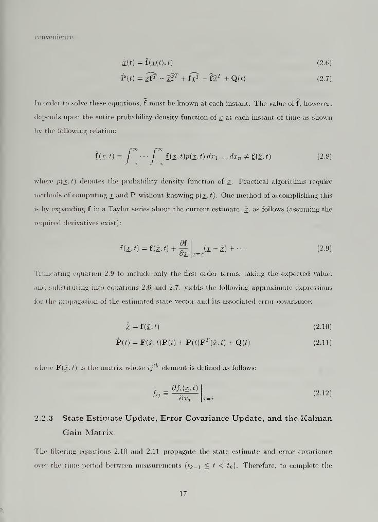
In order to solve these equations, f must be known at each instant. The value off, however.
depends upon the entire probability density function of x at each instant of time as shown
by the following relation:
roc roc
l{x-t)= ••/ i{x,t)p(x,t)dxi...dxn ^i(x,t)I V '- X
12.8)
where p{x.t) denotes the probability density function of x. Practical algorithms require
methods of computing x and P without knowing p{x, t). One method of accomplishing this
i> by expanding f in a Taylor series about the current estimate, x, as follows (assuming the
required derivatives exist):
f(x.t)=f(xJ.) + ^-OX
[x-x) + --- (2.9)
Truncating equation 2.9 to include only the first order terms, taking the expected value.
,iik1 substituting into equations 2.6 and 2.7. yields the following approximate expressions
for the propagation of the estimated state vector and its associated error covariance:
i = f{x.t) (2.10)
P(t) =F(x.t)P(t)+P{t)FT (x.t) + Q(t) (2.11)
where F(x.t) is the matrix whose ijth element is defined as follows:
dfAx.t)jlj - dx
:2.i2)
2.2.3 State Estimate Update, Error Covariance Update, and the Kalman
Gain Matrix
The filtering equations 2.10 and 2.11 propagate the state estimate and error covariance
over the time period between measurements {tk-\ < t < tk). Therefore, to complete the
17


filter and update the state estimate for the next time step, the actual state measurement
must he taken into account. Because the EKF algorithm produces a minimum variance
estimate of the state vector, there will likely be a difference between the propagated state
estimate (denoted £/,.(—
)
4) and the actual measurement (denoted zk ). Thus, the updated
state estimate (denoted xk {+ )) can be computed by a linear combination of the propagated
state estimate and the difference between the actual measurement and propagated state
estimate. The sealing factor in this linear combination is known as the Kalman Gain
matrix. K k . Equation 2.13 illustrates this relation.
xk(+)=xk(-)+Kk [zk -hk (xk (-))] :2.i3)
Measurements affect the error covariance in a manner similar to the state estimate
update. Therefore, denote the propagated error covariance as P k (—
) and the updated
error covariance as P k (+ ). The optimum Kalman Gain matrix, Kk , minimizes the error
covariance update. P k (+ ). Expressing P k ( + ) as a function of of Kk yields the following
expression to be minimized:
Pw( + ) = Pw(-)+K k£ [z k -hk (x k.)]xk (-y :2.i4i
Like the state estimate update. x k (+ ). equation 2.14 is a linear combination of the prop-
agated error covariance and the estimation error. Minimizing equation 2.14 yields the
Following expression for the optimum Kalman Gain matrix (see [19] for details):
Kk = -E x k (-)[z k -hk (xk )]
T E [zk -hk (xk )][z k -hk (x k )}
: + Ri (2.15;
Note that hk depends upon the entire probability density function of x(t) similar to f in
2.2.2.° Employing the method in 2.2.2 and expanding hk in a Taylor series about the
current propagated state estimate. x k (—
). yields the following expression:
H = hk (^.(-)) + Hk (x k (-))(xk- xk (-)) + (2.16)
'i; ( — ) and Pk( — ) represent the solutions to equations 2.10 and 2.11 on the interval tfc-i < t < tfc.
^Scc equation 2.8.
18

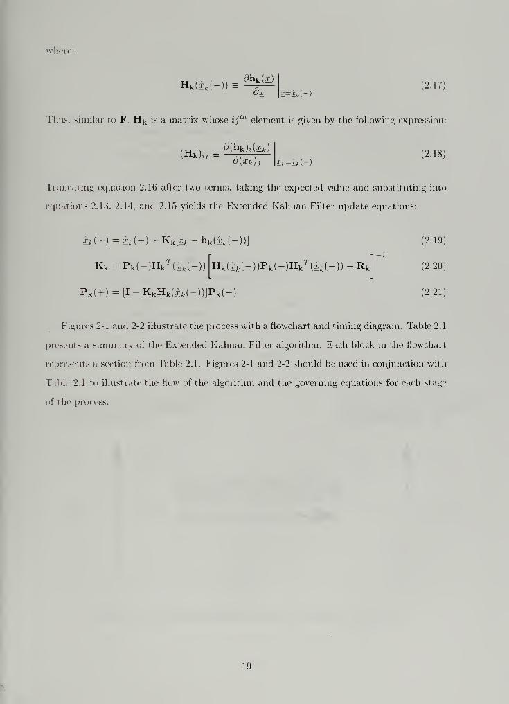
where:
Hk (ijfc(-)) =dx X=Xu(-)
(2.17)
Thus, similar to F. Hk is a matrix whose ij element is given by the following expression:
(Hk)y =d(hk)j(g
fc ;
d(xk )j **=£*(-)(2.18)
Truncating equation 2.16 after two terms, taking the expected value and substituting into
equations 2.13. 2.14. and 2.15 yields the Extended Kalman Filter update equations:
r-i. + = 2±k ±k Kk[^-hk (a.(-))]
Kk = Pk(-)Hkr(ab(-)) Hk (i-,(-))P k (-)Hk
r(^.(-)) + Rk
P k (-) = [I-KkHk (x,(-))]P k (-)
(2.19)
(2.20)
(2.21)
Figures 2-1 and 2-2 illustrate the process with a flowchart and timing diagram. Table 2.1
presents a summary of the Extended Kalman Filter algorithm. Each block in the flowchart
represents a section from Table 2.1. Figures 2-1 and 2-2 should be used in conjunction with
Table 2.1 to illustrate the flow of the algorithm and the governing equations for each stage
of the process.
19


Initial Condition*, and
Assumptions
Solve Plant Model ODE to
compute:
Propagated State Estimate
Propagated Error Covariance
Use Propagated State and Error
Covariance to Compute the
Kalman Gain Matrix
Use propagated state estimate, propagated
error covariance. Kalman Gain, and
actual noisy measurements to compute:
Updated State Estimate
Updated Error Covariance
Take Noisy Measurements
of Actual Plant for
Input to Update Equations
Figure 2-1: EKF Algorithm Flowchart
Take a noise-corruptedmeasurement, \
Take a noise-corruptedmeasurement, ^+1
x, A Xk
( + )
Pk W
A
Solve Plant Model ODEand Error Covariance ODE
xk+i (
'
pk+i(-)
a Xk+ l
(+)
pk+ i
(+)
l
kl
k+l
Figure 2-2: EKF Timing Diagram Adapted from Figure 4.2-1 of [19]
20


Table 2.1: Summary of the Extended Kalman Filter Equations
System Model
Measurement Model
x(t)=f(x(t),t)+w{t)
z k - hk {x{tk )) + v k
Initial Conditions
Othei Assumptions
x(Q) ~ N(x ,-P)
E\w{t)v£ V k and t
State Estimate
Propagation
Error Covariance
Propagation
x = f(x,t) (Plant Simulation Model)
P(/) = F(x, t)P(t) + PitjF 1 {x.t) + Q{t)
State Estimate
Update
Error Covariance
Update
Kalman Gain
xk {+) = xk {~) + Kk [zk- hk (xk (-))}
P k ( + ) = [I-KkHk (i fc(-))]Pk |
Kk = P k (-)Hkr (i,(-))S- 1
(ifc(-))
Definitions m{t),t) = *wtdx(t)
Hk (xfc(-))^^
x{t)=x{t)
S(r,( Hk (i,(-))P k (-)H kT (:r,(-))+Rk
Adapted from Table 6.1-1 of [19]
21


2.3 System Identification of the Esso Osaka
No a priori information on the parameters of the DDG-51 was available in this study. Thus.
if rhf> identification process produced erroneous values of the coefficients, there would be
no definitive method of isolating the problem to the model or the filter. In an effort to
ensure proper operation of the filter prior to use in identifying the DDG-51 hydrodynamic
coefficients, a linear model of the Esso Osaka was developed using coefficient values provided
in [3j.
The Esso Osaka is a 280.000 dead-weight-ton VLCC with principal characteristics listed
in Table 2.2. Abkowitz conducted a series of experiments outlined in [3] in the late 1970's
Table 2.2: Esso Osaka Principle Characteristics
LBP 1066.3 ft
Beam 173.9 ft
Draft 92.8 ft
A r (rudder area) 1289.67 ft2
AR (rudder aspect ratio) 1.538
A 314,410 lton
LCG (aft of midship) 25 ft
and early 1980's to evaluate the EKF technique as a candidate for identification of ship
hydrodynamic derivatives. The study produced favorable results and simulations using the
identified coefficients matched the full-scale data quite well. The successful results presented
in [3] formed the basis for choosing the EKF method in this study.
The mathematical calculations involved in formulating the EKF are quite involved. The
potential for error, therefore, is rather high. Thus, in order to ensure that no mathematical
errors had occurred, it was necessary to test the filter against a dynamical model with
known parameters. Successful operation of the filter in identifying the known parameter
values would indicate that the filter had been properly formulated. The values of the
coefficients appear in Table 2.3. The negative signs have been included in the coefficient
definitions of Yv and Nv to follow the convention outlined in [49].
22


Tabic 2.3: Esso Osaka Nondimensionai Hydrodynamic Coefficients
V, 0.0244
(m - Yr )0.0138
— VA 'J.
(mx - av;
1.4578e-3
8.093e-4
The results of the identification appear in Figures 2-3 and 2-4. These figures clearly
indicate that the filter operates correctly. Notice how the parameter estimates converge to
the exact values of the actual coefficients over time in Figure 2-4. This is indicative of the
fact that the dynamical model in the filter is identical to the dynamical model producing
the measurements. 1 he fact that there are no modeling errors removes the requirement for
process noise (i.e. Q = 0). Thus, the filter trusts its own state estimates and converges
quickly to the proper values based upon the initial measurements. Figure 2-3 shows how the
estimates of the physical states converge immediately. This is due to the exact dynamical
model in the filter and the fact that each of the four physical states are measured. Figure 2-4
indicates that each of the parameter estimates requires about 3 minutes to converge. This is
because each of these states must be estimated by the filter and some dynamic information is
required before the filter can produce good estimates. After about three minutes, the error
between the actual and estimated state vectors has decayed to zero. Thus, the computed
gains are very small and the filter has effectively "learned" the dynamics of the system and
no longer requires measurement information to produce good estimates.
23


Actual
j - Estimated
100 200 300 400 500 600 700 800 900
100 200 300 400 500 600 700 800 900
100 200 300 400 500 600 700 800 900
100 200 jjl 400 500 600 700 600 900
100 200 400 500
time (sec)
Figure 2-3: State Estimates of the Esso Osaka During a 10°/10° Zig-Zag Maneuver
100 200 300 400 500 600 700 800 900
§ op
C 100 200 300 400 500 600 700 800 9()0
100 200 300 400 500 600 700 800 900
100 200 300 400 500 600 700 800 900
time (secj
Figure 2-4: Parameter Estimates of the Esso Osaka During a 10°/10° Zig-Zag Maneuver
24


Results of simulations performed using the identified coefficients appear in Figures 2-
5 and 2-6. The identified coefficients reproduce the states and trajectory with very small
error. This, again, can be attributed to the fact that the filter contained an exact dynamical
model during the identification process. Note also that the trajectory shown in Figure 2-6
is identical to the maneuver used to identify the coefficients.
50C 1000 1500 2000 2500 300
1
-
Figure 2-5: Simulated States of the Esso Osaka During a 10°/10° Zig-Zag Maneuver
Simulation of Esso Osatta 10H0 Zig-Zag Maneuver Using Identified Coefficients
X (yds)
Figure 2-6: Simulated Trajectory of the Esso Osaka During a 10°/10° Zig-Zag Maneuver
25


Figure 2-7 shows the simulation results in a 10° steady turn maneuver. The simulation
results are still quite accurate despite the differing maneuver. The error shown in the figure
is less than b% in the turning diameter. The error can most likely be attributed to roundoff
errors in determining the coefficient values. This small error, however, is certainly ideal for
control system design.
Esso Osaka 10 Degree Steady Turn Maneuver5000 r
Figure 2-7: Simulated Trajectory of the Esso Osaka During a 10° Rudder Steady Turn
26


Chapter 3
Nonlinear Simulation Model
Many of the intricate details of the hullform described in the sequel have been omitted. This
work uses a model developed in [43] to generate the data for the full-scale ship. Classification
restrictions prevent verification of this model against any full-scale data for the DDG-51.
Thus, no attempt has been made here to do so. The focus of this work lies in using the
SAEKF process to identify the unknown parameters in the equations of motion and develop
control systems based upon the identified parameters. The goal then becomes using the
identified values of the 1 parameters to reproduce ship trajectories generated by the model
from [43].
The sequel develops the general equations of rigid-body motion and the assumed form of
the simulation model to be used in the SAEKF. Note that the form of the simulation equa-
tions developed in this study are in no way related to the form of the equations used in [43].
This ensures that the SAEKF does not merely estimate the parameters of a model identical
to that which it contains. In fact, the form of the simulation equations is unimportant as
long as the trajectory of the actual data is reproduced. Thus, the issue of coefficient can-
cellation described in [3] becomes moot. The goal of this study is not to identify individual
coefficient values, but to reproduce trajectories. This implies that the forces and moments
have been adequately modeled, which is the most important factor in control system design.
3.1 The Arleigh Burke Class Destroyer
The United States Navy (USN) Arleigh Burke (DDG-51) Class destroyer represents the
state of the art in operational warships today. It is a twin-screw vessel powered by four
27


LM250C) gas turbine engines coupled to controllable-reversible pitch (CR.P) propellers. The
vessel has a wider beam than conventional warships, but is still considered to have fine
lines. Table 3.1 lists the ship's principal characteristics. The vessel uses two mechanically-
linked rudders located downstream of the propellers to maintain course control. The ship's
propellers maintain 100% pitch for all speeds above approximately 10 knots, and thus will
be considered fixed for the duration of this study. The ship has port-starboard symmetry
as do nearly all ships in existence today.
Table 3.1: DDG-51 Principal Characteristics
Length (LBP) 466 ft
Beam yttj 59 ft
Draft (T) 21 ft
Displacement (A) 8500 lton
Waterplane Area (Aw )29896 ft
2
Long Ctr Gravity (LCG) 2.8 ft aft midship
Block Coeff (C 6 )0.522
Prismatic Coeff (Cp )0.615
3.2 Governing Equations of Motion
3.2.1 Rigid-Body Inertial Forces and Moments
The following sections develop the equations governing the inertial forces and moments ex-
perienced by the body in dynamic motion. Simplifications ultimately reduce the generalized
equations to only those governing motions in the horizontal plane.
3.2.1.1 Generalized Equations of Rigid-Body Motion
The complete derivation of the generalized equations of motion for a rigid body moving on
the surface of the earth begins by choosing an inertial coordinate system with its origin
located at the earth's center of gravity. This is necessary to account for centrifugal forces.
coriolis forces, etc. The body experiences these forces due to the earth's gravitational
field and its relative linear and angular velocity to that of the body. The effects of these
phenomena, however, can be considered small (and thus neglected) for large objects such
as ships. Reference [2] details this portion of the derivation, so it will not be reproduced
28


here.
Based upon the assumptions outlined in [2], the coordinate system is transformed into
a body-fixed reference frame with its origin located at the midship section. Figure 3-1
illustrates the coordinate system in a body-fixed reference frame.
In the most general case, theMotions
ship may exhibit coupled mo-
tions in all six degrees of free-
dom shown in Figure 3-1. All
three forces and all three mo-
liieiit.s shown in Figure 3-1 act-
on the ship during normal op-
erating conditions while under-
way at sea. Equating the forces
and moments acting on the ship
<
J
P
/ Forces and Moments:' X = iree
"i= u
z = heave force
K = = roll moment
M = pitch moment
N == yaw moment
Figure 3-1: Body-Fixed Coordinate System
to the rates of change of linear and angular momentum experienced by the ship yields the
generalized equations of motion shown in equations 3.1 through 3.6.
X = m
Y = m
Z = in
u + qw - rv - xg (q + r2
) + yg (pq— r) + zg (pr + q)
v 4- ru - pw - yg (r2 + p
2) + zg (qr
- p) + xg (qp + r)
t'r + pv - qu - zg {p
2 + q2
) + xg (rp - q) + yg (rq + p)
K = Iyp + {IZ - ly )qr + m
M = Iyq + (Ix — Iz )rp + m
yg (tv + pv — qu) — zg(u + ru — pw
zg(u + qw — rv) — x
g(v + pv — qu)
N = I: r -f (Iy — IT )pq + m\xg(v + ru — pw) — yg (w + qw — rv)
(3.1)
(3.2)
(3-3)
(3.4)
(3.5)
(3.6)
where m represents the mass of the body and IXl ly
. and l z represent the moments of inertia
about the appropriate axis. Because the longitudinal center of gravity is sufficiently close
to the origin, and the ship is nearly symmetric, the cross-coupling inertia terms can be
considered small and neglected.
29

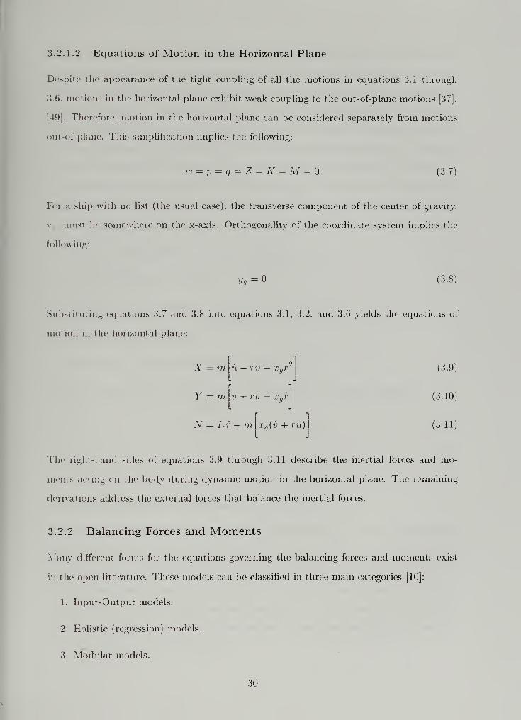
3.2.1.2 Equations of Motion in the Horizontal Plane
Despite the appearance of the tight coupling of all the motions in equations 3.1 through
3.6. motions in the horizontal plane exhibit weak coupling to the out-of-plane motions [37].
19]. Therefore, motion in the horizontal plane can be considered separately from motions
out-of-plane. This simplification implies the following:
w =p = q = Z = K = M = (3.7)
For a ship with no list (the usual case), the transverse component of the center of gravity.
y must lie somewhere on the x-axis. Orthogonality of the coordinate system implies the
following:
y9 = o [3.8)
Substituting equations 3.7 and 3.8 into equations 3.1, 3.2, and 3.6 yields the equations of
motion in the horizontal plane:
X = m
Y = m v + ru + xgr
N = Lr + m Xg[v + ru)
(3.9)
[3.10)
(3.11)
The right-hand sides of equations 3.9 through 3.11 describe the inertial forces and mo-
ments acting on the body during dynamic motion in the horizontal plane. The remaining
derivations address the external forces that balance the inertial forces.
3.2.2 Balancing Forces and Moments
Many different forms for the equations governing the balancing forces and moments exist
in the open literature. These models can be classified in three main categories [10]:
1. Input-Output models.
2. Holistic (regression) models.
3. Modular models.
30


Input-output models describe the direct effect of varying control parameters on the maneu-
vering response of the ship. Holistic models treat the ship as a complete entity with forces
and moments described by a Taylor series expansion containing the pertinent kinematic and
geometric parameters. Modular models treat all major contributing elements as separate.
interactive modules which can be developed and tested separately. Developments over the
last decade indicate that the flexibility of the modular approach makes it very attractive
for future applications [10]. Thus, this type of approach has been adopted in this work.
The following sections develop the equations governing the forces and moments 1 which
balance the inertia] forces and moments derived in 3.2.1. The total force and moment can
bi subdivided into forces and moments resulting from the following modular contributions:
1. External influences (wind, waves, etc.), Xext . Ytx t- Nex t.
2. Steady-state effects. Xq, Yq, Nq.
3. Propulsive devices (propellers, tnrusters, etc.), Xp. Yp, Np.
4. Rudder forces. Xr, Yr, Nr.
5. Interactions between the fluid and the hull. Xf, Yf, Nf.
Thus, the total forces and moments may be described by the following equations:
X = Xext + X + Xp + XR + Xf(3.12)
Y = Yext +Y + Yp + YR + Yf (3.13)
N = Next + N + Np + NR + Nf (3.14)
3.2.2.1 External Forces and Moments
This study considers maneuvering only in calm, deep water with no wind or current effects.
This is not a likely operational environment for a full-scale ship. The goal of this study,
however, is to reproduce maneuvering trajectories produced by the model developed in
[43]. No environmental forces were considered in that study and therefore will not be
considered here. Once the SAEKF method proves effective in the absence of environmental
forces, the next logical step would be the addition of environmental forces to determine
X. V. and N from equations 3.9 through 3.11.
31


their effects. Therefore, A',,,. }",,,. and Next are taken to be zero for the duration of
the identification portion of this work. These effects will be considered, however, dining
simulation of controller designs. This is not a limitation because a scale model may be
tested in a pool or tank where the environment can be carefully controlled to perform the
identification.
3.2.2.2 Steady-State Effects
Steady-state effects consist of forces and moments present in steady-state motion. Thus, the
steady-state Xq is taken to be the ship resistance at the steady-state forward speed when
ither dynamic terms are zero Y< and !V represent steady-state sway force and yaw
moment, respectively. These phenomena exist primarily on single-screw ships and mani-
fest themselves through a tendency for the ship's stern to "walk" in a particular direction
when the propeller thrust is small. DDG-51 has two shafts and two propellers that rotate
in opposing directions. Thus, for this platform, the steady-state sway forces and yaw mo-
ments cancel and can be considered zero. Furthermore, because the steady-state forces and
moments cancel, the dynamic forces and moments will cancel as well. Thus.
Y = No = YP = NP = (3.15)
3.2.2.3 Propulsive Forces and Moments
When a ship propels itself through water, the longitudinal force must be equal to the
difference between the hull resistance and the propeller thrust. The open-water thrust
provided by the propeller can be expressed as follows [49]:
2 n4T = pn zD Ko + K,J + K2 J2
(3.1G)
/= „; "
(3.1'nD
where n represents the propeller speed. D represents the propeller diameter, and J represents
the advance coefficient. The constants (Kq, K\, and K2 ) represent the coefficients in a
parabolic fit of the thrust coefficient to the open-water propeller curve and (1 — w) represents
the Taylor wake fraction. Inserting equation 3.17 into equation 3.16 and carrying out the
32


requisite algebra results in the following expression:
T = X, 2 2rjin~ -<r rj^nu + 773« (3.18)
where:
Vl = PD 4K
rl2 = (l-w) PD iKl
m = {l-w)'2 PD 2K2
(3.19)
(3.20)
(3-21)
Modeling of propeller thrust and torque introduces an additional state variable, u.. into
the equations of motion. Appropriate models for this variable depend heavily upon the
type of propulsion machinery the plant contains. The DDG-51 propulsion system consists
of four LM2500 gas turbine engines mechanically coupled to two shafts via a set of reduction
gears. Reference [49] recommends the following form for modeling a gas turbine propulsion
system:
71 =Tlr^VoQE ~ Qp
2irln(3.22)
where Qe and Qp represent the engine and propeller torque, respectively. Ip represents
the polar moment of inertia for the entire engine/gear/shaft/propeller arrangement. A rep-
resents the reduction gear ratio, and r)r and r]g
represent the propeller relative rotative
efficiency and reduction gear transmission efficiency, respectively. This model is intended
only to adequately model the changes in propeller speed during maneuvers. It is not in-
tended to completely capture the performance of the engine itself. Adequate modeling of
propeller speed changes captures the salient dynamics required for maneuvering and tra-
jectory simulation. Therefore, this model suffices for the task at hand. Thus, the engine
model used in this study is the same as that used in [43]2
.
afT + b) +cfr
nmaxQe = Qma
Lnn
Qp= pn 2D^KQ (J)= Pn
2D'° Q0 + Q1J + Q2J*
(3.23)
(3.24)
'Reference [1] provides a more detailed model to capture the performance of the engine.
33

where all coefficients in equation 3.23 are taken directly from [43]. /, represents the fuel
rate, and the constants (Qo-Q\- and Qo) represent the coefficients in a parabolic fit of the
torque coefficient to the open-water propeller curve.
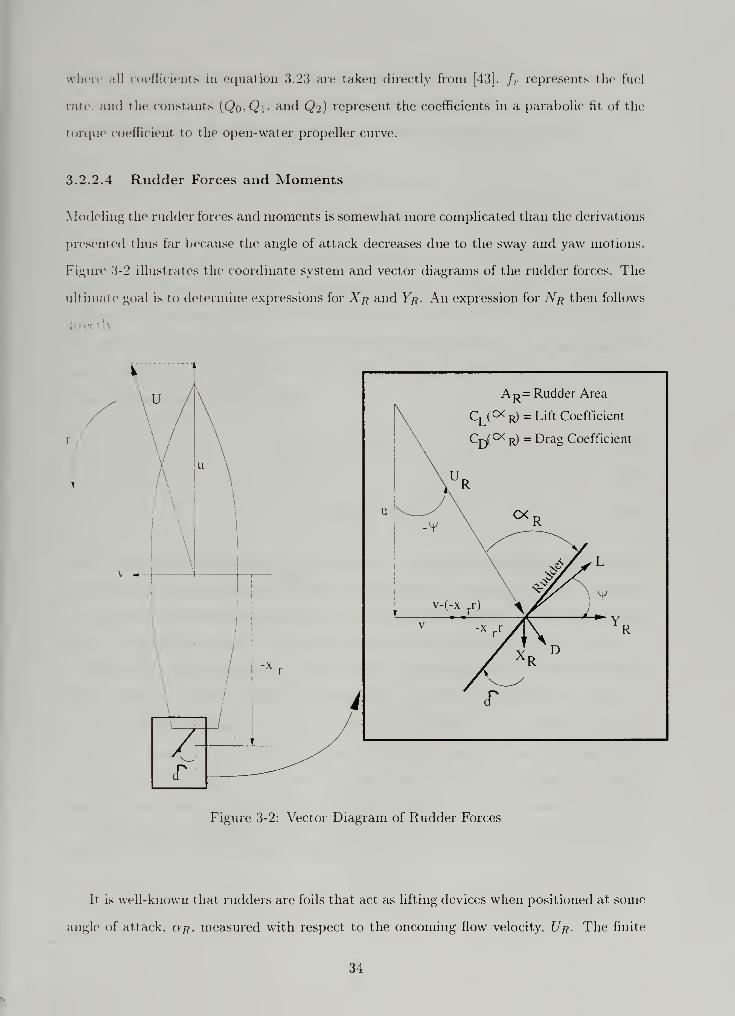
3.2.2.4 Rudder Forces and Moments
Modeling the rudder forces and moments is somewhat more complicated than the derivations
presented thus far because the angle of attack decreases due to the sway and yaw motions.
Figure 3-2 illustrates the coordinate system and vector diagrams of the rudder forces. The
ultimate goal is to determine expressions for Xr and Yr. An expression for Nr then follows
i Iv
r
A^= Rudder Area
CL (°<
r)= Lift Coefficient
Cr/^ r) = Drag Coefficient
Figure 3-2: Vector Diagram of Rudder Forces
It is well-known that rudders are foils that act as lifting devices when positioned at some
angle of attack, or. measured with respect to the oncoming flow velocity. Ur. The finite
34


radius at the leading edge of the foil requires that the lift force. L. act perpendicular to
the oncoming flow [49]. Orthogonality of lift and drag requires that the drag force. D. act
parallel to the flow. The lift and drag forces are defined in equations 3.25 and 3.26.
L =^PARU 2
RCL (a R ) (3.25)
D =l
-pARU 2RCD {a R ) (3.26)
When v and r equal zero. aR is simply the rudder angle, 6. When the ship experiences
sway and yaw motions, however. o R decreases as shown in Figure 3-2 3. The angle ip
represents the decrease in the angle of attack due to swav and vaw. Thus, the instantaneous
lift and drag forces depend upon the instantaneous flow velocity. UR . and instantaneous
angle of attack. a R . The quantities shown in Figure 3-2 are determined from the relations
shown in equations 3.27 through 3.29.
r2 2 , / , „ „x2UR = ir + (v + x r r)z
(3.2
QR =8 + %l) (3.28)
V; = arctan (
V + XtT)
(3.29)
The lift coefficient. Ct(a R ). and drag coefficient. Co{aR ). can be approximated with any
appropriate model. A typical value for the drag coefficient of a foil is 0.0085 [31]. The lift
coefficient can be modeled as a constant for small angles of attack [49]. Use of the modular
rudder model allows the use of this approximation even in maneuvers where it appears to
be invalid (i.e. a 20° rudder turn). This is because the actual angle of attack decreases
rapidly with respect to the nominal as sway speed and yaw rate increase. Reference [3] used
a 20" rudder turn to validate nonlinear coefficients identified in more violent maneuvers.
This can be taken to mean that in that work, this type of maneuver was considered to be
at least mildly nonlinear. The sequel will show, however, that this approximation works
quite well for maneuvers of this type. For foils with aspect ratio (AR) greater than 1. [49]
'Figure 3-2 shows an apparent increase in the angle of attack for illustration purposes only. always
opposes 6 ro allow the forces to balance in steady state.
35


provides the following expression for the linear lift coefficient, C/,:
dCL ( 1 1 1
CtdaR \0.1Stt
+ nAR^ 27r(ARy2 )(3 '30)
Tims, taking Co = 0.0085 and computing Ci from equation 3.30. the lift and drag forces
may he computed from equations 3.25 through 3.29. Once the lift and drag forces are
known, the rudder forces are computed with equations 3.31 through 3.33 where the factor
of two accounts for the fact that the ship has two rudders.
XR = 2{Lsmip- Dcosip) (3.31)
Yr = -2(L cos ip + D sin ip) (3.32)
NR = xrYR (3.33)
3.2.2.5 Hull/Fluid Interaction Forces and Moments
The forces and moments generated by the interaction between the fluid and the hull are
functions of several variables. Thus, Xf< Yf, and Nj may be described by the following
('((nations:
Xf= fi{u,v,r) (3.34)
Yf = f2 (u,v,r) (3.35)
Nf= Mu.v.r) (3.36)
The open literature provides many expressions for f\. f2 , and fo along with detailed deriva-
tions and underlying assumptions 4. The derivations and assumptions will not be repeated
here with the understanding that all equations presented in the sequel conform to all as-
sumptions described in the references from which they were taken.
The major differences between the proposed models lie in their treatment of the non-
linearities. Abkowitz proposed the most well-known form of the equations outlined in [37].
This model proposes a third-order Taylor series expansion of the fluid forces and moments
about some steady-state forward equilibrium speed. Hwang [24] further refined this model
based upon full-scale maneuvering trials conducted on a series of large tanker ships [3].
'Sec [2]. [3]. [7], [13]. [26], [52]. and [54].
36


Blanke [5] proposes a simpler form of the equations intended to capture the most important
uoulinearities in terms of speed and propulsion loss. The form of the simulation equations
chosen for this study is a hybrid of the models proposed in [5] and [24]. It should be noted
that each of the models mentioned here are based upon the holistic method described in
3.2.2. Because this work employs the modular method, the hydrodynamic derivatives asso-
ciated with the rudder forces in these models 3 are captured by the rudder model described
in 3.2.2.4. Thus. f\. /2 , and f% are expressed as follows6 :
Xf= j\ (u. v, r) = Xuii + XP +Xh (3.37)
Yf = f2 (u. v. r) = Y,-,v + Y,r 4- Yh (3.38)
Nf= h [u.v.r) = Ni, v + Nf r 4- Nh (3.39)
Added mass and added inertia terms associated with accelerations (i.e. u, <;. etc.)
can be calculated to within sufficient accuracy for purposes of control systems through
hydrodynamic strip theory. The terms A/t
, Y/,, and N^ in equations 3.37 through 3.39.
however, represent some combination of unknown damping and nonlinear terms whose
values no existing hydrodynamic theory can predict with any level of accuracy. These
terms arc currently determined through extensive model testing. Thus, the linear damping
and pertinent nonlinear terms must be estimated to provide at least some knowledge to be
beneficial in the design of a control system.
3.3 Nonlinear Simulation Equations of Motion
Completing the steps that follow results in the final form for the nonlinear simulation
e([uations of motion.
1. Apply the simplifications and assumptions discussed in 3.2.2.1 through 3.2.2.3.
2. Introduce the resulting expressions for X, Y, and N to equations 3.9. 3.10, and 3.11.
3. Solve the resulting system of equations for the state derivatives and obtain a system
in the state-space form of equation 2.10.
*Xss, Ys, -Va- etc.
''Equations 3.37 through 3.39 employ standard SNAME notation for hydrodynamic derivatives. Thus,
the coefficients in the Taylor series expansion ^, ji, etc. are absorbed by the hydrodynamic coefficients.
See [37] for details.
37


Tin- final model which results from completing each of the steps listed above appears in
Table 3.2. Coefficients of added mass and added inertia terms in Table 3.2 are determined
from valid hydrodynamic theory and knowledge of the ship geometry. Coefficients of the
linear damping terms and any nonlinear terms (i.e. components of X/,. Y/, . and TV/,) are to
bo treated as the unknown parameters to be estimated using the SAEKF.
Table 3.2: Nonlinear Simulation Equations
Vh
III - Xy
(1\ - Ni)h - {jnxg- Yr )h
t
'
f4
[in - Yi,)f3 - (rnxg - Nv )f2/
uh
_ rirXrjgQE - Qp2tvIp
I
h = run2 + ri2nu + n^u 2 + Xh + Xr
h = Yh + YR
h = Nh + NR
h = (I: -Nr )(m-Y,-,)- [mxg - Yf){mxg- Nit )
'/i = pD'Kq
n-2= (1- w)PD :iK l
m = (1 -w) 2pD 2K2
Coefficients of inert ial terms such as V, and Nt to be determined from hydrodynamic theory.
Pertinent term s in Xi, Yi, and Nh to be estimated with SAEKF.
38


Chapter 4
DDG-51 System Identification
Effective control system design relies upon simplified models that adequately describe the
dominant dynamics of the plant to be controlled. These simplified models must contain the
minimum number of parameters required to sufficiently describe the forces and moments
acting on the plant. The equations developed in Chapter 3 are intended to describe the
complete nonlinear plant dynamics. The dominant forces and moments are often captured
by linear terms over a surprisingly wide range, however. Modern control system theory
provides the capability to design controllers that are robust in the face of modeling errors.
Thus, the first step in design is to design a controller based upon a linear model and test
its performance on the nonlinear plant.
The linear ship dynamics are governed by added mass and added inertia terms, as
well as linear damping terms [37]. Hydrodynamic theory provides sufficiently accurate
methods for calculating the former. Plant stability, however, is governed by the latter, for
which no theory provides sufficiently accurate results. These terms must be determined
experimentally. Several experimental methods for determining these terms are outlined in
137]. The drawback to these experimental methods is that they require expensive equipment
and labor in addition to a scale model to collect the necessary data. A method of determining
these terms using only the scale model is one of the focal points of this study.
4.1 Linear Ship Dynamic Equations
Ships operating at sea most often conduct maneuvers that lie within the linear regime. For
example, ships in normal operating conditions do not usually use very large rudder angles
39


in rmns. The most common rudder angles are often between 10-15°. This type of maneuver
lirs well within the linear regime. During such maneuvers, forward speed loss and propeller
rotational speed loss are small. They do exist, but for the purposes of control system design.
they are sufficiently small such that they do not significantly effect the performance of the
controller. This implies that the surge equation, ii, and the propeller speed equation, h,
in Table 3.2 are uncoupled from the sway equation, v, and the yaw equation, r. Thus, the
identification process reduces to the determination of fi and f%.
Table 3.2 shows that /2 and fa each contain two terms which describe the hull damping
forces and the rudder forces. The rudder force model developed in 3.2.2.4 is based solely
upon wing theory and the kinematics of rhe problem. Thus, this force is assumed to be
accurately modeled and requires no identification. Therefore, the identification problem
reduces to determining the hull damping forces, Yj, and N/t
. Abkowitz [37] suggests that
in the nonlinear case, these terms are adequately modeled with a third order Taylor se-
ries expansion. This expansion, however, contains a very large number of terms which is
intractable from a control system perspective. For linear maneuvers, however, the expan-
sion may be truncated after the first order terms. This truncation leads to the following
expressions for fj and fa-
f2 = -Yvv-{m-Yr)r (4.1)
f3 = -Nvv - (mxg - Nr)r (4.2)
Thus, for the case of linear maneuvers, the identification problem is reduced to the deter-
mination of the parameters —Yv ,(m - Yr ), —Nv , and (mxg - Nr ). The negative sign on Yv
and Nv was introduced to maintain the convention outlined in [49] that —Yv should have a
large positive value.
4.2 Initial Identification
The 10"/ 10° zig-zag maneuver proposed in [3] was used to determine the linear coefficients.
This type of maneuver lies well within the linear regime and also provides "persistence
of excitation". Reference [34] states that "An open-loop experiment is informative if the
input is persistently exciting." This effectively states that the system dynamics must be
40


continually excited in order to get any information about the parameters. A steady turn,
for instance, would quickly reach a steady state and provide no more dynamic information
to update the filter. Thus, persistent excitation is crucial to successful identification.
Recall that the model generating the measurement data was taken from [43]. This model
was adapted from a form proposed by Inoue in [26]. The model is parametrically based on
full-scale data obtained from experiments performed over a range of operating conditions.
The model suffers, however, during a simulated zig-zag maneuver. The implementation of
the model in [43] suffers from a drift effect due to the rudder model. Figure 4-1 illustrates
this effect.
20.
|Actual
|
\ -
-20 L V -
-40 -
-60
-80 -
-100
: i
\j
1000 1500
X (yos)
Figure 4-1: 10"/ 10" Zig-Zag Maneuver Using the Rudder Model in [43]
Initial attempts at identifying the coefficients using this model produced biased results.
Because no a priori information was available for the value of the unknown parameters, the
only way to determine success or failure of identification was through simulation. Figures
4-2 and 4-3 show the values obtained through identification and the resulting simulation.
4.2.1 Bias and Divergence in the Extended Kalman Filter
Divergence and bias in the Kalman Filter is well-documented in the open literature. Diver-
gence and bias, however, do not imply filter instability. The EKF possesses some guaranteed
41


Parameter Estimates
Figure 4-2: Parameter Estimates Using the Rudder Model from [43]
Simulated"
"raiectory
i
! Actuai
j
- Identified[
700 j-
/
-
600I
I
/
-
500 /
/
i
(yds)
*>8/
/
1-
300 r
/
s
/
-
2001-s
100 1-
I
'
600 600X (yds)
Figure 4-3: Trajectory Simulation Using the Rudder Model from [43]
42


stability properties under a few mild conditions [20]. Thus, the filter can exhibit "appar-
ent divergence" [12] and give incorrect (biased) parameter estimates. References [12] and
[44] propose that bias is caused primarily by errors in the filter model. This suggestion is
well-supported by [14] and [30]. Reference [22] provides numerical examples of the effects
erroneous models can have on the performance of the filter. Each of these suggest that
the model of the plant used in the filter must be sufficiently close to the actual plant to
guarantee reliable results.
The process noise covariance matrix. Q. used in the filter model is meant to account for
modeling errors. Thus, the choice of Q represents a critical filter design parameter. If the
[)i icess noise is chosen too small, the filter "learns" the wrong state values too well. This
means that the error covariance decays too rapidly and the filter ignores any additional
information contained in the measurements. Thus, the process noise may be said to "drive"
the filter and ensure that it does not place undue weighting on its own estimates. Increasing
the process noise, however, has a strong effect on the convergence of the filter. Thus, it can
nor be chosen too high or the filter will not converge. In an effort to account for the bias,
identifications were attempted using a wide range of process noise values ranging from
and covering two orders of magnitude. Similar results were obtained in all cases.
Much work has gone into developing an analytical method for determining the process
noise covariance. Reference [4G] proposed a method for handling noise covariances through
post-processing of data. References [18]. [39]. and [40] all propose methods for estimation
of the covariances in real-time. Friedland proposes another method for estimating the bias
terms in real-time in [14].
4.2.2 Treatment of the Biased Estimates
Favorable application results were demonstrated in each of the works cited above. Ap-
plication of these techniques to the ship maneuvering problem, however, has not been
demonstrated to the author's knowledge. The most favorable application of the SAEKF
technique to the ship maneuvering problem is summarized in [3], which is the culmination
of 10 years of research conducted at the Massachusetts Institute of Technology (MIT). The
details are outlined in the combined works of [6], [21], [24], [35], and [47]. It is evident in [24]
that bias was a problem as well, although it is not explicitly described. In that work, the
assumed form of the simulation model was significantly altered from the Taylor expansion
43


form proposed in [2] and [37] to obtain favorable results.
This rationale has been adopted in this work as well. The drift illustrated in Figure 4-3
most likely results from numerical problems in the model from [43] due to its parametric
nature. The linear dynamics of ship maneuvering are well-documented and the assumed
form shown in equations 4.1 and 4.2 are not likely to be overly erroneous. For these reasons,
the rudder model used in [43] was replaced with the rudder model derived in 3.2.2.4. Any
further references to this model assume this modification has been made.
4.3 Identification of the Linear Damping Coefficients
4.3.1 Noise Parameters
The magnitude of the process noise covariance matrix, Q. and the sensor noise covariance
matrix. R. determine the weighting the filter applies to its own estimates and the measure-
ments, respectively. During the course of the study, the trade-off between the two became
evident. Given the sophistication of current digital modern measurement devices, the non-
dimensional measurement noise was chosen in all cases as R = 0.01I 1. When the process
noise is too small, the filter trusts" its own estimates too much and. thus, gives a very low
weighting to the measurements (i.e. low gains). This introduces the bias discussed in 4.2.1.
Figures 4-4 and 4-5 illustrate this phenomenon.
The identification uses the nonlinear model from [43] to generate the data and the filter
employs the linear model described in 4.1. Figure 4-4 shows that the states are apparently
tracked quite closely. Note, however, that the filter never updates the surge speed, ?/,. This
is caused by the fact that the absence of process noise implies perfect modeling of the plant
dynamics. Therefore, the filter has no reason to update its own propagated estimates (i.e.
low gains). The close tracking of the sway speed, t>, and the yaw rate, r, indicate that the
nonlinear terms in these equations contribute very little during a linear maneuver. This
indicates that the dynamics are modeled with sufficient accuracy. Thus, the filter is justified
in trusting its own propagated estimates.
Figure 4-5 shows the parameter estimates during the identification. Note how each of
the parameters converges nicely to a constant value. This indicates that the error covariance
'This value is of the same order of magnitude as the non-dimensional forces, which is believed to he
con.seivative.
44


Stale Estimates with 0=0
150 200
time (sec)
Figure 4-4: State Estimates During a 10°/ 10° Zig-Zag Maneuver with Q=0
Parameter Estimates with Q=0
Figure 4-5: Parameter Estimates During a 10°/10° Zig-Zag Maneuver with Q=0
45


has decayed to zero and the filter stops updating the estimates. Recall the expression for
the gams. K^. from Table 2.1. This equation implies the following:
Ki as P k ( 0^ x k ( + ) =x k {-) (4.3)
The results in Figure 4-5 are misleading, however, since they exhibit apparent, divergence
[12]. Figure 4-6 illustrates the results of the simulation after identification. The steady turn
is chosen as the simulation maneuver to illustrate the performance of the filter estimates in
a maneuver other than that used to identify the coefficients. Figure 4-6 shows that, while
Simulation After Identification with Q=0IOC
-40C -300
Figure 4-6: Simulation of a 10° Rudder Steady Turn with Q=0
the filter does converge, the estimates produce an unstable plant.
If perfect modeling of the system dynamics were possible, and the estimates still proved
to be biased, the designer may introduce some "fake" noise into the system. This "fake"
noise would continue to drive the parameters once the state estimates have converged and
cause the filter to weight the measurements more heavily. This technique is outlined in [18]
and suggests that a value of 0.1% of the nominal parameter value is suitable for this purpose.
This approach fails, however, for two reasons. First, using a "nominar parameter value
implies some a priori knowledge of the plant. In this case, as in most cases in the physical
world, this does not exist. Second, because the non-dimensional parameter values are small,
46


once the state estimates have converged the weighting on the measurements will be very
small as well. Thus, the small weighting on the measurements tends to drive the filter very
slowly. Thus, it will not converge in any reasonable period of time. Figure 4-7 illustrates
the effect of the "fake" noise. Note how the parameters appear to be slowly decaying with
time. The slope is so gradual, however, that the filter will require an unacceptable amount
of time to converge (if it does at all).
Parameter Estimates witn Q=0 and "Fake" Noise
50 100 150 200 250 30
/
/'
0.2
' ' i
300
Figure 4-7: Parameter Estimates
Given the previous considerations, the appropriate noise parameters must consist of
some combination of process noise and "fake" noise such that the filter continues to utilize
the information contained in the measurements. The appropriate combination of these noise
parameters was chosen through an iterative process of identification and simulation. Large
process noise was required to effectively track the states. This large process noise, however,
caused rapid convergence to the true state values. Thus, "'fake" noise was also required to
continue to drive the parameters to their true values. The combination of the two noise
parameters allowed the filter to update its dynamical model, as well as obtain information
from the measurements until a balance was achieved. The measurement noise was chosen
as described in 4.3.1. The final values of the noise parameters are listed in Table 4.1.
47


well. The filter also does an excellent job of tracking the sway speed, v, and yaw rate. r.
This, again, is due to the fact that sway and yaw are measured quantities and the process
noise is high. Further, because the nonlinear effects are small in this type of maneuver, the
dynamic model for these two terms is quite accurate.
4.3.3 Parameter Identification
The tour additional states in the filter represent the unknown parameters to be estimated.
Previous sections demonstrated the filter's ability to track the physical states closely, while
giving inaccurate (biased) parameter estimates due to modeling errors and erroneous as-
uoise si tisti s Th iterative process if identification and simulal
produced the parameter estimates illustrated in Figure 4-9.
DDG-51 Estimated Hydrodynamic Coefficients During a 10°/10cZig-Zag Maneuver
-0.1
04
k-Y =5.41e"
3
V
-
)0o 50 100 150 200 250 3C
(m-Y) = 1.51e~
Figure 4-9: Parameter Estimates During a 10°/ 10° Zig-Zag Maneuver
With the exception of 5>. the parameter estimates exhibit variations about some value.
This could prove to be problematic if the goal of the identification were to establish exact
coefficient values. The goal of control system design is to develop controllers that perform
well with only an approximate knowledge of the coefficients. In fact, parameters that model
the state values within 40% of the actual values often leads to acceptable control system
performance. Fortunately, this goal is often achieved. Thus, to determine the coefficient
value to be used in the simulation, the mean value of the last 67% of the parameter estimates
49


was taken to be the parameter value,
4.3.4 DDG-51 Simulation After Identification
The ultimate goal of an automatic maneuvering control system on a ship is to provide a
reliable method of maintaining a desired trajectory. Linear control system theory has been
proven to be quite reliable in designing control systems for plants in which nonlinearities are
weak. Control of an inverted pendulum represents an excellent example of this assertion 2.
Because ship maneuvers normally lie within the linear regime, where nonlinear effects are
small, a control system design based upon a linear ship model could very likely perforin quite
l-lf) and 1-11 illustrate the simulation results using the identified parametei
values.
Simulated Stales After Identification
0-81-
06-
Actuai
Identified
100 200 300 400 500 6C
[V
I I '
600
600
Figure 4-10: Simulated States During a 10° Rudder Steady Turn
Figure 4-10 shows that the identified model tracks the actual nonlinear model quite
closely in sway and yaw. It does not. however, track surge and propeller revolutions at all.
This is because the simulation model ignores forward speed loss and propeller speed loss
(i.e. u = ii = 0). This is a good assumption because the actual speed loss in the simulation
is about 20% and propeller speed loss is approximately 10%. These represent ideal errors
for the application of linear theory to a nonlinear physical system. The lack of speed loss
"See example 2.1-1 in [33].
50


Simulates Trajectory After identification
800
700
600
500
i 400
-
>
300
200
100^
IActual^-~"—— 4 "
—
- s^ ~^^|
- loentitied
^^
/ - * - -
/ y " Error = 15% ^ ^ \/ -" ^ \/ / \ \
_ / • \ \ -/ / \ \/ / \ \
-
/
\ \ -
\ I
-
V!
\
i /
i /
/ /
/ /- \ \ //
/// y
- \v
i
-500 -400 -300 -200 -100 100 200 300 400 500
X (yds)
Figure 4-11: Simulated Trajectory During a 10° Rudder Steady Turn
accounts for the higher values of sway and yaw. Higher speed in a turn implies a tighter
turn, and thus, higher values of sway and yaw.
Figure 4-11 shows the trajectory produced by the identified model. The error in the
ruining diameter between the identified and actual models is approximately 15%. This
situation is ideal for the application of linear control theory to develop automatic controllers
for the ship. Note that the identified model has a tighter turning diameter than the actual
model. This was expected due to the higher values of sway and yaw shown in Figure 4-10.
The identified model maintains higher speed throughout the turn. Thus, it has a smaller
turning diameter.
51


Chapter 5
Controller Design
The previous chapters focused on the identification of the linear damping terms in the
DDG-51 equations of motion. The identification process resulted in determination of the
hydrodynamic coefficients that produce the dominant forces and moments during linear
ship maneuvers. Thus, these terms may be employed to develop simple models which may
form the basis for simple course-keeping controllers.
The sequel describes the design of two controllers based upon simplified ship models.
The first controller is a heading autopilot. The second controller regulates the lateral
deviation (cross-track error) from the desired reference trajectory. The desired frequency
responses are developed using a loopshaping technique. The desired control laws are then
determined from the design loopshape. Simulations are then performed on the nonlinear
ship model using the linear controllers to evaluate their performance.
5.1 Controller Design via Loopshaping
Controller design via loopshaping is well-documented in many texts on feedback and optimal
control system design. More detailed versions of the following presentation are described in
[11]. [33]. and [53].
The overall goal of controller design via loopshaping is illustrated in Figure 5-1. The
Loop Gain should be designed such that the closed-loop plant exhibits robust performance
[Hi. This means that the entire system (plant and controller) exhibit good performance
and tracking at low frequencies within the system bandwidth. The system must also be
robust to high-frequency disturbances such as sensor noise and unmodeled dynamics. The
52


Loop Gain
dB
Figure 5-1: The Goal of Loopshaping
sequel describes how this process is accomplished by the control system engineer.
5.1.1 Feedback Control
Figure 5-2 represents a typical feedback control system with the plant disturbance input.
(I. reflected to the plant output as in [33]. Reference [11] considers the feedback loop with
the disturbance reflected at the plant input. The derivation of [33]. however, makes the
effect of the disturbance and desired properties of the loopshape a bit more clear. Thus, it
is primarily that, derivation that will be presented here.
d
V C -6-
a.
Figure 5-2: Typical Feedback Loop
The goal of a feedback control system is for the plant output, y, to asymptotically track
a desired reference output, r. The plant, P, however, is acted upon by disturbances, d.
which represent external disturbances and modeling errors. Further, the measurements of
the output are influenced by sensor noise, n. The goal of the controller. C, is to compute
53


the control input, u. that regulates the output and maintains the desired reference value
despite the disturbances and measurement noise. Defining the tracking error, e, as follows,
e-r-y (5.1)
examination of Figure 5-2 gives rise to the following expressions:
v = r — y — n (5-2)
y = PCv + d (5.3)
5.1.2 System Sensitivity, Cosensitivity, and Loop Gain
To illustrate the ideas behind loopshaping theory, one requires expressions for the closed-
loop transfer function relations of the desired outputs, y and e. to the deterministic and
stochastic inputs. r, d. and n respectively. Substituting equation 5.2 into equation 5.3
results in the following expression for y
y = PC(r-y-n) + d (5.4)
(I + PC)y = PC(r-n) + d (5.5)
y = (I + PC)-'l PC{r - n) + (/ + PC)~ l
d (5.6)
y = PCil + PC)~ l(r - n) + (7 + PC) _1
d (5.7)
where 1 the final operation is justified because PC is square and invertible [33]. The expression
for the error, e. may be derived in a similar manner.
e = r - PCv - d (5.8)
e = r- PC(r -y- n) - d (5.9)
e = r -d- PC(e-n) (5.10)
(I + PC)e = r-d + PCn (5.11)
e = (/ + PC'r l
{r - d) + (/ + PC)~ yPCn (5.12)
e = (/ + PC)- l(r -d) + PC{I + PCy l n (5.13)
Equations 5.14. 5.15, and 5.16 define the system sensitivity, S", cosensitivity, T, and loop
54


gain. L. respectively.
S = (I + PC)~ 1(5.14)
T = PC(I + PCr 1
(5.15)
L = PC (5.16)
Notice that S + T = /. Thus. S and T may not both be made arbitrarily large. Substituting
equations 5.14 and 5.15 into equations 5.7 and 5.13 results in the following expressions for
the output, ij. and the tracking error, e:
ij = T(r -n) + Sd (5.17)
e = S{r-d)+Tn (5.18)
System disturbances are low-frequency phenomena such as wind and wave forces exerted
on the ship hull. Examples of high-frequency phenomena are sensor noise and structural
vibrational modes. The goal of the controller is to respond to low-frequency disturbances
within the bandwidth of the system and attenuate disturbances outside the system band-
width where its behavior is not as well-known. For example, the controller should respond to
wave disturbances to maintain the desired output, but should not respond to high-frequency
structural vibrational modes whose dynamics were neglected in the system model.
At low frequencies, equations 5.17 and 5.18 may be expressed as follows:
ysaTr + Sd (5.19)
e^S(r-d) (5.20)
At high frequencies the same equations may be represented as follows:
y^-Tn (5.21)
e^Tn (5.22)
because' the reference signal is typically a constant or at least slowly-varying. Thus, the
system sensitivity. S. should be small at low frequencies where the disturbances, d. are sig-
nificant to ensure small tracking errors. Additionally, if S is small. T « 1 at low frequencies
55


(because 5 + T = 1) such that // ~ r. Conversely, the system cost nsitivity, T. should be
small at high frequencies where sensor noise and other high-frequency phenomena are sig-
nificant. If these conditions are satisfied, the controller will exhibit robust performance [11].
This implies that, the controller provides good tracking of reference inputs (performance)
while simultaneously rejecting high-frequency signals where the plant model is not so well
understood (robustness).
5.1.3 Performance Specifications
Frequency-dependent weighting functions are required to establish the low and high fre-
i! ncy performance bounds shown in Figure 5-1. These functions establish the minimum
and maximum open-loop system gains over all frequencies. Thus, one weighting function
should be large (i.e. large positive gains) at low frequencies to ensure good performance.
The other weighting function should be small (i.e. negative gains) at high frequencies to
ensure robustness.
Determination of these weighting functions, coupled with design of the loop gain. L.
then allows development of frequency-domain performance specifications. The idea behind
performance specifications may be illustrated on a Nyquist plot [11] as in Figure 5-3. For
Figure 5-3: Nyquist Plot of Performance Specifications
56


good tracking, the loci of L must lie outside the disk of radius W\ over all frequencies. To
ensure robustness in the face of multiplicative plant uncertainties, the disk of radius H'2
must not pass through the point — 1 -+- Oj over all frequencies.
The goal of the controller is robust performance which implies good tracking and distur-
bance rejection at low frequencies and attenuation of high-frequency signals such as sensor
noise and modeling errors. Recall that the system sensitivity function. S. should be small
at low frequencies to provide good performance and the system cosensitivity function. T
.
should be small at high frequencies to provide robustness. Considering Figure 5-3 and the
definitions of the quantities derived previously, it can be shown [11] that the frequency-
domain performance specification that ensures robust performance is given by the following
expression:
\W,S\ + \W-?T\ < 1 Vu; (5.23)
5.1.4 Design Criteria
The length between perpendiculars (LBP) for the DDG-51 class ships is 466 feet. The main
low-frequency phenomena in the open sea that influence the ship motions consist of waves
and current. Currents are most often constant or at least very slowly varying. Thus, waves
represent the phenomena that regularly contain a frequency component.
The frequency of open-ocean gravity waves is related to their characteristic wavelength.
The motion of the ship is also related to this wavelength. According to [49], the closed-
loop system should respond to wavelengths of the same order as the ship LBP. Thus, the
closed-loop system should respond to all wave disturbances of length 400 feet or greater.
This corresponds to a characteristic circular frequency of 0.7 radians/second (Period % 9
seconds). To allow for some flexibility in the loopshaping, the design crossover frequency.
u)c , should lie in the range between 0.5 - 1.5 radians/sec.
Currents tend to "blow" the ship off course in the same way that wind blows an airplane
off its intended course. If this disturbance is not accounted for, the ship would move far from
its intended track. Thus, the ship must adjust its heading angle such that it accounts for the
drift effect due to the current. Because currents are very low frequency disturbances, the
closed-loop system must track them very accurately. Thus, the closed-loop system should
track disturbances with an error. (3. less than 1% at frequencies below 0.01 radians/sec.
57


This corresponds to open-loop system gains of at least 40 dB below 0.01 radians/sec. Thus.
the open-loop system gains should lie above the low-frequency performance bounds and
below the high-frequency performance bounds illustrated in Figure 5-1 while achieving a
reasonable closed-loop step response. The ultimate test of any controller design is how it,
operates on the actual rather than the nominal plant. The reasons for not specifying time
domain performance criteria will be addressed in the sequel.
5.2 Autopilot Design
The goal of a ship autopilot is to maintain the ship's actual heading around some slowly-
varying reference heading. The autopilot must perform this function in the presence of
disturbances, sensor noise, and modeling errors described in 5.1. The design speed for all
simulations is 22 knots. This corresponds to the maximum ship speed in a plant config-
uration with two of the four main engines on-line, one driving each shaft (split plant).
Nbn-dimensionalization of the equations, however, allows this speed to be adjusted without
affecting the results. The split plant configuration is required, however, to validate the
assumption in Chapter 3 that the steady-state forces and moments due to the propeller
cancel.
5.2.1 Dynamic Model
Low frequency ship motions may be described by a first-order model attributed to Nomoto
[13]. This model may be represented as follows:
TM) + (/' = K6 (5.24)
where </' represents the ship heading angle and S represents the rudder angle. Note that
the sway dynamics have been removed from the equation of motion. T and K represent
the ship time constant and gain, respectively. These terms may be determined from the
hydrodynamic coefficients identified in Chapter 4 using the procedures outlined in section
58


5.3.2 of [13]. This loads to the following values for T and K:
T = 1.9287 (5.25)
if = 2.04 (5.26)
Tims, the plant transfer function. P \ from input. 5, to output, ip. appears in equation 5.27
and represents the change in heading angle to a change in the rudder angle.
s[Ts + 1)
Tin ship's rudder contains its own dynamics. Fur instance, the rudder dues not in-
stantaneously change its angle when commanded by the helmsman. According to [24]. the
rudder dynamics do not play a major role in the identification process because they are
much faster than the ship dynamics. For control purposes, however, the rudder dynam-
ics do play a role. Classification restrictions prevent the disclosure of the actual DDG-51
rudder swing rate. Thus, it was assumed in this work that the rudder dynamics could be
modeled by the following transfer function. Psg , that maps the commanded rudder angle to
the actual rudder angle:
Psg = £ = -?- (5.28)d c s -+-
Thus, the new plant. P. may be represented as follows:
P = PolPsg (5.29)
This new plant. P. corresponds to the plant block in Figure 5-2. To guard against unrea-
sonably large rudder angle commands during maneuvers, a rudder command angle limiter
was added to the model as well. This limits the maximum allowable commanded rudder-
angle during maneuvers to 30°. This guards against the actual rudder angle approaching
the physical stops on the actual ship. The goal now is to design the controller, C, using
loopshaping to achieve robust performance.
59


5.2.2 Loopshaping Controller Design
In some instances, it is possible to shape the loop gain. L. to obtain the desired frequency
response. The controller may then be determined as follows:
C =^ (5.30)
In other cases, the controller must be designed directly to obtain the desired response. The
autopilot design followed the former procedure. The open-loop plant, P. is straight-line
stable [37] as are many ships. Thus, the controller is not required to stabilize the plant.
To give this a physical representation, imagine the ship without any control encounters
a current. The current will cause an initial yaw rate. but. the large wetted surface area in
the stern will develop forces and moments that counteract the initial rate of yaw. Thus, the
yaw rate will decay back to zero after a finite period. Because the heading angle is simply
integral of the yaw rate, or
ip = r (5.31)
flic ship will turn to a heading that faces the current and stay on that heading when r — 0.
Thus, the goal of the autopilot must be to ensure that, the ship continues on its desired
heading despite the current.
Thus, the loop gain for the autopilot, design may be modeled simply as a second-order
system with an integrator whose transfer function may be represented as follows:
L = PC =, , ^n
j- (5.32)s(6'
2 + 2Cu; r( +u;2)
ujn =^ (5.33)
C = 2 (5.34)
Figure 5-4 illustrates the results of the loopshaping design. The loopshape has gains of
at least 40 dB at frequencies below 0.01 radians/sec. It lies above the low-frequency per-
formance bound indicated by W\. This indicates good tracking and disturbance rejection
at low frequencies. The loop gains roll off at high frequencies indicating good attenua-
tion of high-frequency signals and unmodeled fast dynamics. They further lie below the
60


_oopshape 'or Autopilot Design
s-«l-Max = -0.0201 dB -
\
w,
w = 0.9 rad/s
\— —S&^L
'
V^S + W2T ^C
^Qoocoooccoaw
2
\
frequency iraa/sea
Figure 5-4: Loopshape for Autopilot Design
high-frequency performance bound indicated by W2. The design also satisfies the robust
performance requirement given by equation 5.23.
An indication of overall plant stability may be obtained from the Bode plot. Figure 5-5
indicates a gain margin of approximately 30 dB and a phase margin of approximately 64".
Reference [49] indicates that a good rule of thumb for gain and phase margins are 3 dB and
30°. respectively. Thus, the autopilot design falls well within the acceptable range.
Gain ana Phase Margins lor Aulopilol Loopshape
Gm=29 823 dB (at 7 746 rad/secj Pm=64 406 deg (at 91463 rad/sec)
Frequency Irad/sec]
Figure 5-5: Gain and Phase Margins for Autopilot Design
61


The frequency response of a controller is not its only measure of suitability to the task.
The designer must also check the time domain response to ensure adequate closed-loop
performance. Reference [36] indicates that acceptable performance for an autopilot is met
by the following conditions:
1. No more than 5% overshoot to a step input.
2. 2"A settling time less than 5 ship lengths at design speed.
Figure 5-6 indicates that the autopilot design meets these criteria. Additionally, the tracking
error at steady-state is less than 1% as dictated by the frequency response.
Closeo-Looo Steo Response for Autopilot
Z) d - 2% Settling Time = 4
Tracking Error < 1%
Ship Lengths at Design Speed
Figure 5-6: Closed-Loop Autopilot Step Response
5.2.3 Closed-Loop Simulations of the Autopilot Design
The true test of a linear controller is how well it performs in conjunction with the nonlinear
plant from which it was derived. Incorrect assumptions on the level of uncertainty in the
model may lead to poor performance if the unmodeled dynamics have a strong effect on the
plant. In this case, this would arise if the nonlinearities in the equations of motion have a
strong impact on the dynamics. These nonlinearities are believed to be weak in the ship
maneuvering problem, however, as described in Chapter 4. This proved to be true in this
studv as well.
62


To validate the controller performance, two different simulations were developed. The
first is a simulation of the controller's ability to reject a constant current disturbance equal
to 5 knots. For the second simulation, a maneuver was generated by computing the required
instantaneous heading angle required for the ship to begin on a steady course and speed
and execute a 90" left turn and steady up on the new heading. After a period of steady
operation, the ship then executes a 90° right turn and steadies up on its new heading.
5.2.3.1 Current Rejection Simulation
Figure 5-7 illustrates the ship's actual trajectory in relation to the dead-reckoned trajectory
in the absence of any disturbance. Tho current in this case must be simulated as an initial
condition on the ship's sway velocity, v. due to the fact that the dynamics of position. //.
were neglected. The figure shows that the ship gets "blown" approximately 1/3 of a ship
Autopilot Simulation with Nonlinear Plant Model
Actual Trajectory
Commanded Trajectory
Current = 5 knots
»
Error Approx 0.3 Ship Lengths
-so r
-100
500 1000 1500 2000 2500 3000 3500 4000 4500 5000X (yds)
Figure 5-7: Nonlinear Plant Trajectory During Current Rejection
length off its initial track as a result of the current disturbance. It does, however, return
to its commanded heading angle '. Thus, the controller takes the required action to return
the ship to its intended heading.
'It should he noted that the standard compass rose has been rotated 90° in each of the simulations to
follow. Thus, a heading of 000 in the figures corresponds to a heading of 090 on a standard compass rose.
63


Figure 5-8 illustrates the change in ship heading. The ship is initially turned to the
right due to the side forces and moments generated by the current interaction with the ship
hull. The controller detects the difference between the actual and commanded headings via
noisy measurements and generates commands to the rudder to turn the ship to the left and
return it to its intended heading. The heading angle in the figure appears to be zero. This
is not actually the case, however. The ship actually develops a constant sway velocity that
results in a side-slip angle. Thus, while the figure shows the ship's actual heading equal to
zero, the ship is actually turned at a small angle into the oncoming current to account for
it. Simulations that show the actual heading angle appear in the following section where
th<> rlvnamics of y are included in the simulation.
Autopilot Simulation with Nonlinear Plant Model
Current = 5 knots Actual HeadingCommanded Heading
150 200 250time (sec;
300 350 400
Figure 5-8: Nonlinear Plant Heading Change During Current Rejection
64


Figure 5-9 demonstrates the commanded and actual rudder angles during the current.
rejection simulation. The commanded rudder angles may seem excessive at first glance.
The figure shows, however, that, during the maneuver, inclusion of the rudder dynamics in
the equations of motion rejects these high-frequency oscillations. Thus, the actual rudder
motion is smooth during the correction. After reaching steady-state, the rudder does exhibit
some high-frequency oscillatory motion. The amplitude of these oscillations, however, is less
than 0.1" over periods of several seconds. This is not deemed to be a severe condition that
would rend to cause excessive wear on the mechanical components.
Autooiiot Simulation witn Nonlinear Plant Moaei
Actual Ruaaer Angle
Oscillations <0.1 over
periods of seconds
/ i
f*™i^F jrTWfir
iw
IOC ;5C 200time isec..
250 350 100
Figure 5-9: Actual and Commanded Rudder Angle During Current Rejection
The reason for these high-frequency oscillations in the commanded rudder angle is illus-
trated in Figure 5-10. Recall that the goal of loopshaping controller design is to ensure that
flu' closed-loop combination of the plant and controller attenuate high-frequency signals.
Because the plant has very small gains at high frequencies, the controller is free to have
rather large gains at these frequencies. Thus, because the input to the controller is the
noisy, high-frequency measurement of the heading angle, the controller responds in kind.
The controller gain at the measurement frequency is approximately 8 dB. Thus, the con-
troller actually amplifies the measurement noise. The plant gain, however, at the same
frequency is approximately -33 dB. Thus, the effect, of the noise on the entire closed-loop
65


Singula' Vaiues of the Controller and Plant
DU
to*•
- -*.,. P
20
" ^,
^—-—""" " C'x
Xx_
' X-20 *x
':%
'x'x
-40X'x
X
-60X\
X-80
.
XXXX.
Frequency (rad/sec;
Figure 5-10: Plant and Controller Open-Loop Gains
system is attenuated.
5.2.3.2 Track-Changing Maneuver
Figure 5-11 shows the dead-reckoned and actual trajectories of the ship during a track-
changing maneuver. The actual nonlinear plant includes the effect of forward speed loss
due to maneuvers. Thus, because the ship loses speed during the turn and experiences
sway motion, it is not capable of completing the tight turn based solely upon kinematic
relations. Further, the goal of the autopilot is only to maintain the desired heading rather
than to regulate the cross-track error. A regulator of this type is described in the following
section. The track error is approximately three ship lengths following the initial turn. This
is reduced, however, during the second leg of the maneuver due to the sway velocity. The
sway velocity in the second leg is opposite that of the initial leg. Thus, the ship actually
moves back toward its dead-reckoned track on the second leg of the maneuver.
Figure 5-12 shows the actual and commanded heading angle during the track-changing
maneuver. The errors in tracking the ramp input account for the cross-track errors in the
trajectory. The tracking error in steady-state, however, is again less than 1%.
66


Autopilot Simulation with Nonlinear Plant Model
DR Track of Commanded8000- Heading Angle
7000 H
i
6000 (-
5000 L
I Ii
3. 4000 j- Error Approx.
j
3 Ship Lengths3000 r
Error Approx. 2 Ship Lengths
Actual Ship Trajectory
-1000 1000 2000 3000 4000 5000 6000 7000 8000 9000
X (yds]
Figure 5-11: Nonlinear Plant Track-Changing Maneuver with Autopilot
B0
20
Autopilot Simulation witn Nonlinear Plant Modei
Tracking Error < 1%
— Actual Heading- Commanded Heading
200 400 60C 800
time (sec)
1000 1200 1400
Figure 5-12: Nonlinear Plant Heading Angle during Track-Changing Maneuver with Au-
topilot
67


Figure 5-13 shows the commanded and actual rudder angles during the track-changing
maneuver. Again, the rudder motion is quite smooth during the major portions of the
maneuver and is not affected by the high-frequency controller commands. Further, notice
that the rudder sweep during the maneuver is approximately 20° over a period of about
throe minutes. Thus, the controller produces a slow, smooth rudder motion for the duration
of the maneuver. The steady-state oscillations are again small and not deemed to cause
excessive mechanical wear.
30
Autopilot Simulation with Nonlinear Plant
I— Actual Rudder Angle
Commanded Rudder Angle
Rudder Swings 20 and backover a 3-minute period
»^rW#
Oscillations < 1°
over a period of
seconds
*iNMr|N
200 400 600 800 1000 1200 1400
time (sec)
Figure 5-13: Actual and Commanded Rudder Angle During Track-Changing Maneuver
68
-.


5.3 Cross-Track Error Controller Design
The goal of the cross-track error controller is to regulate the ship's lateral deviation from
its intended track. The previous section demonstrated that an autopilot is not sufficient for
this purpose. The controller must meet all criteria previously stated.
5.3.1 Dynamic Model
To begin the design of the cross-track error controller, the coordinate system was shifted.
In the new coordinate system, the x-coordinate represents the distance traveled along the
reference trajectory and the y-coordinate represents the lateral deviation from the intended
track. The heading angle now represents the deviation from the desired heading angle along
tin 1 intended track. The new coordinate system is illustrated in Figure 5-14. The kinematic
tX
VwcV
\0f-
Figure 5-14: New Coordinate System for Track Controller
relations governing ship motions in this new coordinate system is given by the following
equations:
x = u cos ip — v sin ip (5.35)
y = usinip + vcosij) (5.36)
69


Linearizing and non-dimensionalizing these equations leads to equation 5.37.
V = $ (5-37)
where the dynamics of sway have again been removed as in 5.2.1. The dynamics of x have
also been removed since it is not a control variable. Thus, differentiating equation 5.37
and inserting the result in equation 5.31 leads to the following expression for the control
variable, //:
V = r (5.38)
Thus, using SISO loopshaping control design theory, the track controller may be designed by
simply adding an integrator to the plant transfer function given by equation 5.29. Thus, the
new plant transfer function that maps the control input. Sc . to the lateral track deviation.
//. becomes:
Py= - (5-39)
g
5.3.2 Loopshaping Controller Design
Plants with double integrators can be problematic for the control systems engineer due to
the phase shift introduced by the two poles at the origin. The two poles introduce a 180°
phase shift in the plant at DC. Thus, because the dynamics of yaw rate, r, behave as a
second-order system, the phase decreases as frequency increases because the plant has slow
poles.
The slope of the loopshape curve as it passes through the crossover frequency (where
the magnitude is one) must satisfy the condition given by equation 5.40.
dL 1— < —r around u = u)c (5.40)aw w z
The phase associated with this condition is -180°. System stability requires that the phase
be greater than this when the magnitude is one. Thus, the closed-loop system will be
unstable if this condition is not met. Thus, the simple loopshaping design described in 5.2.2
may not be employed. In this instance, the controller must have some zeros to add the
70


required phase around the crossover frequency. Thus, the controller design must proceed
by direct design of the controller. C 2. computation of S and T, and verification of the
desired frequency response of the loop gain. L = PVC' . Thus, the general controller transfer
function to start the design may be defined as follows:
C =_ k{s + z\){s + Zo) . . (s + zn )
(s +pi)(a +P2) ...(a +pn )
(5.41]
where n may be as many poles and zeros as required to achieve a desirable loopshape,
subject to the requirement that the transfer function remain proper (degree of numerator <
degree of denominator) [11]. The final controller design may be described by the following
transfer function:
c = 20(s + 0.5)2{s + 6)(s+ 1000)
(a + 11) (5 + 15)(s + 30) 2(5.42)
Figure 5-15 illustrates the loopshape for the cross-track error controller design. The
design proceeded iteratively by adding zeros and poles in the controller to achieve the
desired frequency response properties. Figure 5-16 additionally shows the gain and phase
Loopshape tor Track Controller Design
Frequency (rad/sec)
Figure 5-15: Loopshape for Cross-Track Error Controller Design
"'Zeros and poles may be easily added and modified using the zpk function available in MATLAB.
71


margins
practice.
the syste
associated with the design. Again, the margins fall well within the range of accepted
Not ice in the phase plot of the Bode diagram how the controller adds phase to
m at frequencies below the crossover frequency, thus stabilizing the plant.
Bode Diagrams
Gm=2l.574 dB (at 7.2766 rad/sec), Pm=50 99 deg. (at 0.95135 rad/sec;
Frequency ( rad/sec;
Figure 5-16: Gain and Phase Margins for Cross-Track Error Controller Design
72


Figure 5-17 illustrates the system closed-loop step response. The overshoot and settling
rime in this rase may seem excessive when compared to conventional design practice. Com-
pare, however. Figures 5-17 and 5-6. and consider equation 5.37. It would be extremely
difficult, if not impossible, to command the dynamics of y to be faster than the dynamics
of r because y depends solely upon 0. Thus, its dynamics must be inherently slower. This
physical fact is confirmed by the step response plot. Closed-loop simulation will subse-
quently show, however, that this controller perforins extremely well on the nonlinear plant
with smooth maneuvering trajectory commands.
Closed-Loop Step Response lor Cross-Track Error Controller
Overshoot = 25%
E £<
Snip Lengths at Design Speed
Figure 5-17: Cross-Track Error Controller Closed-Loop Step Response
73

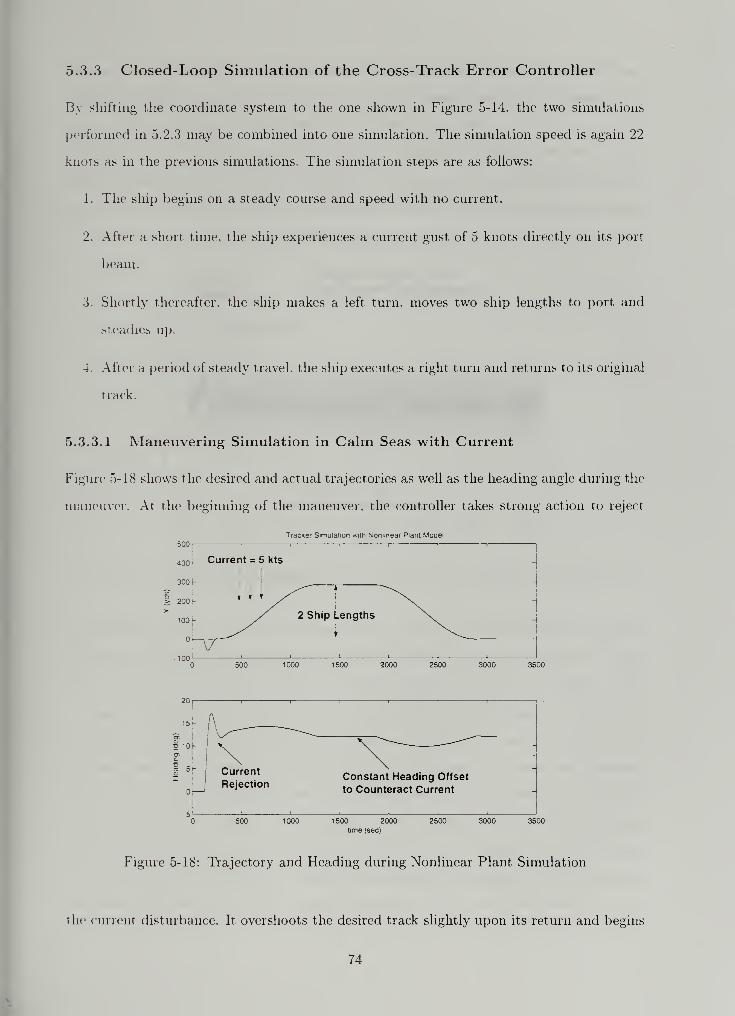
5.3.3 Closed-Loop Simulation of the Cross-Track Error Controller
By shifting the coordinate system to the one shown in Figure 5-14, the two simulations
performed in 5.2.3 may be combined into one simulation. The simulation speed is again 22
knots as in the previous simulations. The simulation steps are as follows:
1. The ship begins on a steady course and speed with no current.
2. After a short time, the ship experiences a current gust of 5 knots directly on its port
beam.
3. Shortly thereafter, the ship makes a left turn, moves two ship lengths to port and
steadies up.
4. After a period of steady travel, the ship executes a right turn and returns to its original
track.
5.3.3.1 Maneuvering Simulation in Calm Seas with Current
Figure 5-18 shows the desired and actual trajectories as well as the heading angle during the
maneuver. At the beginning of the maneuver, the controller takes strong action to reject
TracKer Simulation with Noniinear Plant Model
2 Ship Lengths
H 101-
£ 5I" I Current
|
I RejectionConstant Heading Offset
to Counteract Current
1500 2000
time (sec)
Figure 5-18: Trajectory and Heading during Nonlinear Plant Simulation
the current disturbance. It overshoots the desired track slightly upon its return and begins
74


ro compensate. The left turn then executes and the ship follows the desired track with very
small error until it steadies up. Notice that during the steady parts of the maneuver, the
ship maintains a constant heading offset to counteract the current.
Figure 5-19 shows the commanded and actual rudder angle during the maneuver. The
controller is again seen to respond significantly to the sensor noise for the same reason listed
in 5.2.3.1. The most noteworthy item in this figure, however, is the way the controller senses
Tracker Simulation with Nonlinear Plant Model
Current
Rejection
Initial Left Turn
Controller then Uses Current
During Second Leg of Maneuver
Oscillations +/- 3
over Periods of Seconds
1500
time (sec)
2000 2500 3000
Figure 5-19: Actual and Commanded Rudder Angle During Nonlinear Plant Simulation
the current and uses it to execute the right turn to return to its original track. Note how
the ship's heading decreases slightly below its offset, but does not, pass through zero. Thus,
the controller uses the current to allow the ship to be "blown'" back onto its desired track.
Some may note that the ship requires a great, deal of time (approximately 8 minutes) to
complete the turning maneuvers. This may or may not be desirable. Smooth trajectories are
required, however, to prevent the controller from over-compensating during the overshoot
phase. This application could be extremely valuable, however, in maneuvers to avoid other
vessels. For example, modern radar is capable of identifying contacts well before (longer
than 8 minutes) their closest point of approach (CPA) time. Maneuvers to avoid other
vessels are currently calculated by watchstanders using vector diagrams. Thus, a digital
computer could calculate the CPA. compute a suitable track to avoid the contact by some
75


threshold distance, and then compute a smooth trajectory to maneuver to the new track.
observe CPA. and maneuver back to the intended track.
5.3.3.2 Maneuver in Sea State 4 with 5-Knot Current
The simulation would not be complete without verifying the controller's performance in a
sea state. The sea state is modeled as a random disturbance and filtered to preserve only the
low-frequency components. Table 6 of [38] indicates that a state four sea has a significant
wave height of 1.25-2.5 meters (4-8 feet). Additionally, Table 3 of [38] indicates that waves
of this height represent sea conditions with the highest probability of occurrence worldwide.
is. sea state four was chosen for simulation Figure 5-20 shows the wave spectrum and
Figure 5-21 shows the time history of the wave heights.
Pow«f Specirumo W<jwe Mooei
' f\
'
\1
'
Ho. 1
0< 02 03 04 OS 06 "* 06 0$
Figure 5-20: Power Spectrum of Wave Model
pus lor Wave D'Hu'Mnc* Mooe'
SOO 1000 1500 2000 2500 3000
Figure 5-21: Time History of Wave Heights
76


The same maneuver described in 5.3.3 is performed with the current and sea stare
introduced as disturbances. Figure 5-22 shows the actual and commanded trajectories as
well as the heading angle during the maneuver. Notice that, similar to the maneuver in
calm seas, the controller maintains a constant heading offset to counteract the effects of the
current. The low-frequency wave disturbances, however, cause the ship to deviate from its
commanded track. Thus, the ship oscillates a small amount about its commanded track.
The amplitude of the oscillations, however, is less than 20 yards (about 15% of the ship
length).
Tracker Simulation with Nonlinear Plant Model
500
1
400h
300-
B 200
Current = 5 kts
i i
Sea State 4
Actual Track (-)
Commanded Track (-.)
1000 1500 2000 2500 3000
20
Similar Heading OffsetWave Disturbance
Rejection
500 1000 1500
time (sec)
2000 2500 3000
Figure 5-22: Trajectory and Heading During Track Change
77


Figure 5-23 shows the commanded and actual rudder angles during the maneuver. Care-
ful examination of Figure 5-23 indicates a low-frequency signal among the high-frequency
measurements driving the controller. It is this low-frequency command signal that allows
the ship ro remain on track despite the disturbances.
Tracker Simulation with Nonlinear Plant Model40
30
3o<
T3
CC
-30
Current
RejectionSmall Periodic Motions
Due to Wave Disturbance
Rejection
Oscillations +/- 3°
over Periods of Seconds
500 1000 1500
time (sec)
2000 2500 3000
Figure 5-23: Commanded and Actual Rudder Angle during Track Change
78

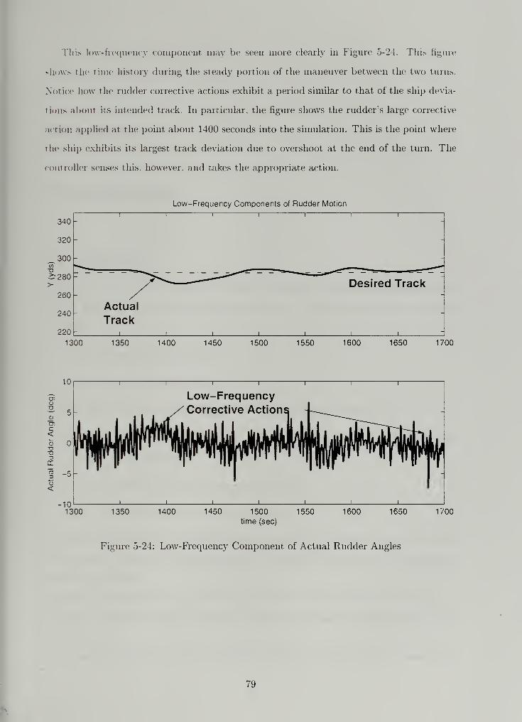
This low-frequency component, may be seen more clearly in Figure 5-24. This figure
shows the rime history ("luring the steady portion of the maneuver between the two turns.
Notice how the rudder corrective actions exhibit a period similar to that of the ship devia-
tions about its intended track. In particular, the figure shows the rudder's large corrective
action applied at the point about 1400 seconds into the simulation. This is the point where
the ship exhibits its largest track deviation due to overshoot at the end of the turn. The
controller senses this, however, and takes the appropriate action.
Low--Frequency Components of Rudder Motion
340i i
i i ii
-
320 -
_300 -
-^280> / Desired Track
_
260 / -
240Actual
Track-
220 i i i 1 1 ! 1
-
1300 1350 1400 1450 1500 1550 1600 1650 1700
10
enCD
c<CD
X3"O
<
-10'
—
1300 1350
Low-FrequencyCorrective Action;
1400 1450 1500 1550 1600 1650 1700
Figure 5-24: Low-Frequency Component of Actual Rudder Angles
79

Chapter 6
Conclusion
6.1 Summary
This work gives rise to a systematic method for adding automatic maneuvering control
system design to the macroscopic ship design process. The procedure may be summarized
as follows:
1. Build a scale model of the ship.
2. Outfit the model with sensors.
."J. Conduct a series of controlled maneuvers with the model to gather data.
4. Design a SAEKF and use the data collected from the model to identify the ship
hydrodynamic coefficients.
•"). Use the identified coefficients to develop controllers.
6. Test the controller designs on the scale model.»6*
This work accomplishes a piece of this process by identifying the linear damping derivatives
and developing control laws based upon them. Specifically, this work accomplished the
following objectives:
• Selection of an assumed form of the equations of ship motion in the horizontal plane.
• Design of a SAEKF to identify the linear damping hydrodynamic coefficients within these
equations.
• Successful identification of these coefficients which are the most critical to overall ship
80

maneuvering stability in the horizontal plane.
• Design of two simple controllers that may be tested on scale ship models to determine
theii performance.
The current method of identifying these terms involves large towing tanks and rotating
arm basins. It also requires extensive labor to operate the equipment. These requirements
are in addition to the need for a scale model of the ship. Thus, development of the ideas
introduced in [3] and [43] and continued here may not only lead to an efficient, effective
process for adding maneuvering automation to the ship design process, it may also reduce
the infrastructure required to support it.
6.2 Conclusions
The following list summarizes the items deemed most noteworthy by the author over the
course of this study.
1. The EKF method shows definite feasibility as a method to determine linear ship
hydrodynamic coefficients. These parameters may then form the basis for simple
controller designs that can be tested on scale models.
2. The parameter estimates provided by the SAEKF need not be very accurate to pro-
vide values suitable for controller design. The parameters determined in this study
reproduced simulation trajectories with approximately 15% error in steady turning
diameter. Errors as large as 40%. however, may very likely yield acceptable controller
designs for slow maneuvers.
3. The dynamics of sway need not be considered to develop effective linear controllers
for the types of maneuvers considered in this study. Thus, controller designs for these
types of maneuvers may be based on only two parameters.
4. The EKF perforins extremely well as a state estimator (due to the physical state
measurements) despite significant inaccuracies in the filter dynamic model. Specifi-
cally, the SAEKF model used in this study was completely linear, but still produced
very accurate estimates of the physical states (u, v. r, and n) of the nonlinear plant
model used to generate the measurement data. The dynamics of u and n, in fact,
were completely ignored in propagating the filter state estimates.
81


5. The performance of the SAEKF as a parameter estimator, however, will degrade if the
alter model is not sufficiently accurate in describing the actual plant. The modeling
errors will cause significant bias in the parameter estimates.
(i. The instantaneous rudder angle of attack decreases rapidly with respect to the nominal
angle of attack as sway speed and yaw rate increase. Thus, the linear lift coefficient
assumption proved to be valid in the maneuvers conducted in this study despite the
use of rudder angles traditionally believed to lie outside the linear regime.
6.3 Recommendations for Further Study
As in any other design study, this work leaves several areas that require further thought and
development. Among these, the most important in the author's mind may be summarized
as follows:
1. This work considers performing the identification in calm water. Environmental dis-
turbances such as wind and waves could have a significant effect on the identification
process. The magnitude of these effects should be investigated.
2. Rolling motions have an effect on maneuvering in the horizontal plane. Thus, the
inclusion of rolling motions in the nonlinear model could have an effect on the linear
controller performance. The magnitude of these effects should be investigated.
3. Despite the identification of four terms in this study, these four terms were reduced to
two to develop the controllers. Identification of only these two terms using an SAEKF
may be possible. This could make the implementation of the SAEKF much simpler.
4. The EKF provided very accurate estimates of the surge speed and propeller rotational
speed despite the fact that its model completely ignored their dynamics. These quan-
tities are easily measured by the speed log and a shaft tachometer. Thus, perhaps the
EKF could be used to provide state estimates for a MIMO controller to control the
ship's x-coordinate as well as its y-coordinate.
5. The proper noise covariance terms are an important design parameter in any Kalman
filter implementation. This study determined the correct noise covariances through an
iterative procedure of identification and simulation. Inclusion of the noise covariances
82


as filter parameters to be estimated may reduce the iterative nature of this process
and lead to a more efficient design process.
6. Implement the method outlined herein on the DDG-51 scale model developed at the
MIT Towing Tank.
7. Investigate the range over which the assumption of linearized lift on rudders is valid
by accounting for the ship dynamics in computing the instantaneous angle of attack.
83


Appendix A
State Augmentation of the
Extended Kalman Filter
The derivations presented in section 2.2 hold for estimation of the state vector describ-
ing a nonlinear system. Augmentation of the state vector for use in estimating unknown
parameters is the subject of the sequel.
Recall equations 2.10 and 2.19 in 2.2.2 and 2.2.3, respectively. The variable x represents
tin estimate of the states describing the physical system. Therefore, the estimated state
vector can be augmented with the unknown parameters in the system to allow them to be
estimated along with the system states. In the case of DDG-51. the unkown parameters arc'
constant hydrodynamic maneuvering coefficients. Maneuvering coefficients may change with
changes in submerged geometry, speed, etc. Nondimensionalization of the equations removes
speed considerations and submerged geometry certainly changes slowly with time. DDG-
51"s compensated fuel system, however, ensures that the ship maintains nearly constant
draft over its entire range of operation. Therefore, the state vector is augmented with
the unknown system parameters whose derivatives are zero. For example, to estimate an
unknown parameter, b. in a system fully described by states x\ and X2, the state vector and
84


Appendix A
State Augmentation of the
Extended Kalman Filter
The derivations presented in section 2.2 hold for estimation of the state vector describ-
ing ;i nonlinear system. Augmentation of the state vector for use in estimating unknown
parameters is the subject of the sequel.
Recall equations 2.10 and 2.19 in 2.2.2 and 2.2.3, respectively. The variable x represents
the estimate of the states describing the physical system. Therefore, the estimated state
vector can be augmented with the unknown parameters in the system to allow them to be
estimated along with the system states. In the case of DDG-51, the unkown parameters are
constant hydrodynamic maneuvering coefficients. Maneuvering coefficients may change with
changes in submerged geometry, speed, etc. Nondimensionalization of the equations removes
speed considerations and submerged geometry certainly changes slowly with time. DDG-
51 "s compensated fuel system, however, ensures that the ship maintains nearly constant
draft over its entire range of operation. Therefore, the state vector is augmented with
the unknown system parameters whose derivatives are zero. For example, to estimate an
unknown parameter, b. in a system fully described by states x\ and x'2, the state vector and
84


associated F matrix would be augmented as follows:
b
F =
fi(xi,x2 ,0,t)
f2(xi,x2 ,P,t)
dh dfi djidxi d.i:-: c)i
dfo df2 dfjdx\ dx> 813
A.l
(A.2)
Using this methodology, an initial estimate is made for the unknown parameters in the
augmented stat< vector and the associated error in the estimate. Tin parameters are then
estimated in exactly the same manner as the state vector. Once the state vector has been
augmented with the unknown parameters, and the F matrix modified appropriately, the
EKF becomes the SAEKF. The following section presents an example application of the
SAEKF.
85

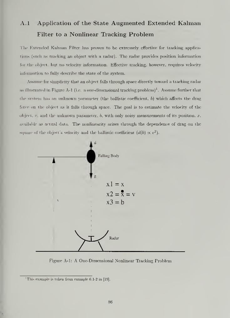
A.l Application of the State Augmented Extended Kalman
Filter to a Nonlinear Tracking Problem
The Extended Kalman Filter has proven to be extremely effective for tracking applica-
tions (such as tracking an object with a radar). The radar provides position information
for the object, but no velocity information. Effective tracking, however, requires velocity
information to fully describe the state of the system.
Assume for simplicity that an object falls through space directly toward a tracking radar
as illustrated in Figure A-l (i.e. a one-dimensional tracking problem) 1. Assume further that
the system has an unknown parameter (the ballistic coefficient, b) which affects the drag
force on the object as it falls through space. The goal is to estimate the velocity of the
object, i". and the unknown parameter, b. with only noisy measurements of its position, x.
available as actual data. The nonlinearity arises through the dependence of drag on the
square of the object's velocity and the ballistic coefficient {d(b) oc v 2).
Falling Body
xl = X
x2 = x = v
x3 = b
Radar
Figure A-l: A One-Dimensional Nonlinear Tracking Problem
This example is taken from example 6.1-2 in [19].
86


Figure A-2 illustrates the results. The upper plot shows the filter's ability to very
accurately estimate the object's velocity as it falls through the atmosphere. The lower plot
illustrates the filter's ability to converge on the true value of the ballistic coefficient using the
measurements and computed gains. The filter does not change much initially because the
object experiences very little drag high in the atmosphere. As the object enters the dense
atmosphere the filter converges to the true value and remains there. Thus, one concludes
that the filter has difficulty identifying the parameter value if it does not significantly affect
the dynamics.
-5900
-6000
S.-6100
-6200
-6300 -
-6400
Actual Velocity
- Estimated Velocity
14 16
3000 r
2500
— 2000 -
O 1500o
= 1000(0
CD
500 -
Actual Ballistic Coefficient
Estimated Ballistic Coefficient
8 10
Time (sec)
12 14 16
Figure A-2: EKF Application
87


References
[1] PDI Report 336091-01. Design and Analysis of an Alternative Programmed Control
Module (PCM) for DDG-51 Class Ships". Technical report, Propulsion Dynamics. Inc..
February 1994.
[2] M. A. Abkowitz. Lectures in Ship Hydrodynamics, Steering, and. Maneuverability. MIT
Press. Cambridge. MA, 1964.
[3] M. A. Abkowitz. Measurement of Hydrodynamic Characteristics from Ship Maneu-
vering Trials by System Identification. SNAME Transactions, 88:283-318. November
1980.
[4] B. D. O. Anderson and J. B. Moore. Optimal Filtering. Prentice-Hall. Inc.. Englewood
Cliffs, NJ, 1987.
"i M. Blanke. Ship Propulsion Losses Related, to Automated. Steering and Prime Mover
Control. PhD thesis. The Technical University of Denmark. Lyngby. Denmark. 1981.
[6] H. L. Brinati. System Identification Applied to Maneuvering Trials. Master's thesis.
Massachusetts Institute of Technology, Department of Ocean Engineering. 1973.
[7] J. Chudley et al. A review of mathematical model used in ship manoevers. In Pro-
ceedings of Computer Methods in Marine and Offshore Engineering. Florida. USA.
1991.
[8] D. L. Coble. A Flight Test Sutdy to Determine Aircraft Propulsive Efficiency and Aero-
dynamic Drag Using an Extended Kalman Filter Parameter Identification Technique
and Lock's Propeller Model. Master's thesis, Mississippi State University, Department
of Aerospace Engineering. 1992.
88


[9] E. Z. Chios. Use of the Modified Gain Extended Kahnan Filter in the Identification
of Aircraft Stability Derivatives. Master's thesis. The University of Texas at Austin.
Austin. Texas. 1985.
10] I. W. Dand et al. Report of the manoenverability committee. In Proceedings of the
2(P International Towing Tank Conference, pages 309-361, Seoul, Korea. 1993.
Ill] .1. C. Doyle et al. Feedback Control Theory. Macmillan Publishing Company. New
York, XY. 1992.
[12] R. J. Fitzgerald. Divergence of the Kalman Filter. IEEE Transactions on Automatic
Cuiii vol. AC-16:73b 747. December 1971.
[13 T. I. Fosscn. Guidance and Control of Ocean Vehicles. John Wiley & Sons. New York.
XY. 1994.
[14] B. Friedland. Treatment of Bias in Recursive Filtering. IEEE Transactions on Auto-
matic Control. AC-14:359X367. August 1969.
[15] B. Friedland. Control System, Design: An Introduction to State-Space Methods.
McGraw-Hill. Inc.. New York. NY. 1986.
[16] W. P. Fun. An Explicit Adaptive Flight Control System Based on the Modified Gain
Extended Kahnan Filter. Master's thesis. The University of Texas at Austin, Austin.
Texas. 1986.
[17] .1. B. Garcia- Yolo. Parameter Estimation of an Unstable Aircraft Using an Extended
Kahnan Filter. Master's thesis. University of Cincinnati, Department of Aerospace
Engineering and Engineering Mechanics. 1991.
[18] J. B. Garcia-Velo. Determination of Noise Covariances for Extended Kalman Fil-
ter Parameter Estimators to Account for Modeling Errors. PhD thesis. University of
Cincinnati. Department of Aerospace Engineering and Engineering Mechanics, 1997.
[19] A. Gelb et al. Applied Optimal Estimation. MIT Press. Cambridge, MA, 1974.
[20] D. B. Grunberg. Guaranteed Properties of the Extended Kalm.an Filter. Massachusetts
Institute of Technology. Cambridge, MA, 1987.
89


21 M. N. Hayes. Parametric Identification of Nonlinear Stochastic Systems Applied to
Ocean Vehicle Dynamics. PhD thesis, Massachusetts Institute of Technology. Depart-
ment of Ocean Engineering. 1971.
[22] H. HefFes. The Effect of Erroneous Models on the Kalman Filter Response. IEEE
Transactions on Automatic Control. AC-1 1:541-543, July 1966.
23] T. Holtzhtiter. A workable dynamic model for the track control of ships. In Proceed/mas
of fh, 9th Ship Control Systems Symposium,, pages 4.275-4.298. Maryland. USA. 1990.
2 1 W. Y. Hwang. Application of System Identification to Ship Maneuvering. PhD thesis.
Massachusetts Institute of Technology, Department of Ocean Engineering. 1980.
25] S. Inoue et al. Hydrodynamic derivatives in ship maneuvering. International Ship-
building Progress. 28:112-125, No. 321 1981.
[26] S. Inoue et al. A practical calculation method of ship maneuvering motion. Interna-
tional Shipbuilding Progress. 28:207-222. No. 325 1981.
[27] R. Isermann et al. Adaptive Control Systems. Prentice Hall, New York, NY. 1992.
[28] C. G. Kallstrom et al. A track autopilot predictor system for ships. In Proceedings of
the 11" 1 Ship Control Systems Symposium. Southampton^ UK. 1997.
[29] R. E. Kalman. A New Approach to Linear Filtering and Prediction Problems. Transac-
tions of the American Society of Mechanical. Engineers. Journal of Basic Engineering.
32:34 35. March 1960.
[30| R. E. Kalman and R. S. Bucy. New Results in Linear Filtering and Prediction The-
ory. Transactions of the American Society of Mechanical Engineers, Journal of Basic
Engineering. 83:95-107. December 1961.
[31] .1. E. Kerwin. Class Notes for Propellers and Hydrofoils. Massachusetts Institute of
Technology. Cambridge. MA. 1996.
[32] O. Kohei et al. A Robust Autopilot System Against the Various Sea Conditions: Noise
Adaptive Autopilot. Ship Operation Automation. 7, March 1979.
90


•'5.5 F L. Lewis. Applied Optimal Control and Estimation. Prentice Hall. Englewood Cliff's.
X.I. 1992.
[34] L. Ljung. System Identification: Theory for the User. Prentice-Hall. Inc.. Englewood
Cliffs. X.I. 1987.
[35] I. G. Lundblad. Application of the Extended Kalman Filtering Technique to Ship
Maneuvering Analysis. Master's thesis. Massachusetts Institute of Technology, De-
partment of Ocean Engineering. 1975.
[36] Driels M. Linear Control Systems Engineering. McGraw-Hill. Inc., Xew York, XY.
1996.
[37] P. Mandel et al. Principles of Naval Architecture. SNAME, Chapter 9. Section 2, 1988.
[38] P. Mandel et al. Principles of Naval Architecture. SXAME, Chapter 8. Section 2. 1988.
39 R. K. Mehra. On The Identification of Variances and Adaptive Kalman Filtering. IEEE
Transactions on Automatic Control. AC-15:175-184. April 1970.
[40] T. Xishimura. On the A Priori Information in Sequential Estimation Problems. IEEE
Transactions on Automatic Control. AC-11T97-204. April 1966.
141] X. H. Xorrbin et al. The Identification of Linear Ship Steering Dynamics Using Max-
im inn Likelihood Parameter Estimation. Swedish State Shipbuilding Experimental
Tank. Goteborg. Sweden. 1975.
[42] C. L. Phillips and R. D. Harbor. Feedback Control Systems. Prentice-Hall. Inc., Upper
Saddle River. X.l. 2000.
[43] R. E. Quezada Ojeda. Robust Control Design and Simulation of the Maneuvering
Dynamics of an Arleigh Burke Class Destroyer. Master's thesis. Massachusetts Institute
of Technology. Department of Ocean Engineering, 1999.
[44] F. H. Schlee et al. Divergence in the Kalman Filter. AIAA Journal, 5:1114-1120, June
1967.
[45] M. M. Sidar and B. F. Doolin. On The Feasbility of Real-Time Prediction of Aircraft
Carrier Motion at Sea. IEEE Transactions on Automatic Control, AC-28:350- 355.
March 1983.
91


46; T. T. Soong. On A Priori Statistics in Minimum-Variance Estimation Problems. Trans-
actions of the American Society of Mechanical Engineers. Journal of Basic Engineering,
87:109 112. March 1965.
47] F. F. Szeto. System Identification Techniques for Ship Maneuvering Trials. Master's
thesis. Massachusetts Institute of Technology, Department of Ocean Engineering. 1977.
18] L. S. Taek. A Stochastic Analysis of a Modified Gam Extended Kalman Filter. PhD
Ihesis, The University of Texas at Austin. Austin. Texas. 1984.
19 M. S. Triantafyllou. Class Notes for Maneuvering and Control, of Surfa.ce and. Under-
watei Vehicles. Massachusetts Institute of Technology, Cambridge. MA. 1996.
[50] J. Van de Vegte. Feedback Control Systems. Prentice Hall. Englewood Cliffs. N.I. 1994.
[51] -1. Wunnenberg. Convergence of the Extended Kalman Filter. Master's thesis, Univer-
sity of Washington. Seattle. Washington. 1985.
[52] Y. Yansheng. Study of ship maneuvering mathematical model in shiphandling simu-
lator. In Proceedings of MARSIM and ICSM. pages 607-615. Copenhagen, Denmark.
1996.
53 K. Zhou and .7. C. Doyle. Essentials of Robust Control. Prentice Hall. Upper Saddle
River. N.I. 1998.
54 W. Zhou. Identification of Nonlinear Marine Systems. Servolaboratory. Technical
University of Denmark. Lyngby. Denmark. 1987.
92

69 ^re
eiflii6/02
290NPG*
TH
22527-200 nlb