synthesis of regional wildlife and vegetation field ... · synthesis of regional wildlife and...

Synthesis of Regional Wildlife and Vegetation Field Studies to GuideManagement of Standing and Down Dead Trees

Bruce G. Marcot, Janet L. Ohmann, Kim Mellen-McLean, and Karen L. Waddell

Abstract: We used novel methods for combining information from wildlife and vegetation field studies todevelop guidelines for managing dead wood for wildlife and biodiversity. The DecAID Decayed Wood Advisorpresents data on wildlife use of standing and down dead trees (snags and down wood) and summaries of regionalvegetation plot data depicting dead wood conditions, for forests across the Pacific Northwest United States. Wecombined data on wildlife use by snag diameter and density and by down wood diameter and cover, acrossstudies, using parametric techniques of meta-analysis. We calculated tolerance intervals, which represent thepercentage of each species’ population that uses particular sizes or amounts of snags and down wood, andrank-ordered the species into cumulative species curves. We combined data on snags and down wood from�16,000 field plots from three regional forest inventories and calculated distribution-free tolerance intervalscompatible with those compiled for wildlife to facilitate integrated analysis. We illustrate our methods using anexample for one vegetation condition. The statistical summaries in DecAID use a probabilistic approach, whichworks well in a risk analysis and management framework, rather than a deterministic approach. Our methodsmay prove useful to others faced with similar problems of combining information across studies in other regionsor for other data types. FOR. SCI. 56(4):391–404.

Keywords: forest inventory, snags, down wood, tolerance interval, meta-analysis

MANAGING STANDING AND down dead trees (snagsand down wood) in forests for wildlife and biodi-versity requires knowing how wildlife use dead

wood and how conditions of forest vegetation relate to thoseuses. In the Pacific Northwest United States and elsewhere,information on wildlife species’ use of dead wood resides inmany disparate field studies. In a wildlife-habitat relation-ships database, O’Neil et al. (2001b) summarized wildlifeuse of dead wood in Washington and Oregon, but in termstoo general and qualitative to guide management decisionsat local and watershed levels. At the other extreme, detailedhabitat capability models have been developed for individ-ual, focal wildlife species that use dead wood (e.g., Mc-Comb et al. 2002), but such models lack applicability tobroader communities of wildlife species. Furthermore,many assumptions underlying existing conceptual modelsthat were used to develop agency standards and guidelinesfor managing dead wood for wildlife have been invalidatedover the last 20 years (Rose et al. 2001).

In managing forests for broader ecological goals, includ-ing wildlife, it is also useful to know how dead wood variesacross a forest landscape as a function of forest develop-ment, disturbance history, and environment. Vegetationconditions in wildlife habitat types in Washington and Or-egon are sampled in regional forest inventories, but data on

snags and down wood are collected with different sampledesigns and methods and have not been summarized acrossall ownerships and vegetation conditions for the explicitpurpose of comparing with wildlife use in particular wildlifehabitat types.

Limitations of Existing Approaches forAssessing Wildlife–Dead Wood Relations

Models of relationships between wildlife species andsnags in the Pacific Northwest typically are based on cal-culating potential densities of bird species and expectednumber of snags used per pair. This approach was first usedby Thomas et al. (1979). Marcot expanded this approach inNeitro et al. (1985) and in the Snag Recruitment Simulator(Marcot 1992) by using published estimates of bird popu-lation densities instead of calculating population densitiesfrom pair home range sizes. This approach has been criti-cized because the numbers of snags suggested by the mod-els seem far lower than are now being observed in fieldstudies (Lundquist and Mariani 1991, Bull et al. 1997). Inaddition, the models provided only deterministic point val-ues of snag sizes or densities and of population response(“population potential”) instead of probabilistic estimates

Bruce G. Marcot, US Forest Service, Pacific Northwest Research Station—[email protected]. Janet L. Ohmann, US Forest Service, Pacific NorthwestResearch Station, 3200 SW Jefferson Way, Corvallis, OR 97331—Phone: (541) 750-7487; Fax: (541) 758-7760; [email protected]. Kim Mellen-McLean,US Forest Service, Pacific Northwest Region—[email protected]. Karen L. Waddell, US Forest Service, Pacific Northwest ResearchStation—[email protected].

Acknowledgments: We thank Tim Max and Manuela Huso for their statistical review of the use and calculation of tolerance intervals. The senior author alsothanks Scott Overton for teaching theory and use of tolerance intervals in graduate statistical classes at Oregon State University in the early 1980s. We thankthe many researchers and biologists who provided data and peer review of DecAID. We are especially grateful to Martin Raphael for providing conceptualadvice early in the development of our process. We thank the regional inventory programs (FIA, CVS, and BLM) for the wealth of data they provide. AndrewGray and several anonymous reviewers provided helpful comments on earlier versions of this manuscript.

Manuscript received September 30, 2009, accepted February 10, 2010

This article was written by U.S. Government employees and is therefore in the public domain.

Forest Science 56(4) 2010 391

that are more amenable to a risk analysis and risk manage-ment framework.

In addition, existing models have focused on terrestrialvertebrate species that are primary cavity excavators.Thomas et al. (1979) and Marcot (1992) assumed thatsecondary snag-using species would be fully provided for ifneeds of primary snag-excavating species were met. How-ever, McComb et al. (1992) and Schreiber (1987) suggestedthat secondary cavity nesting birds may be even moresensitive to snag density than are primary cavity excavators.Furthermore, existing models do not address relationshipsbetween wildlife and down wood, nor do they account forspecies that use different types of snags and partially deadtrees, such as hollow live and dead trees used by bats(Ormsbee and McComb 1998, Vonhof and Gwilliam 2007),Vaux’s swift (Chaetura vauxi) (Bull and Hohmann 1993),American marten (Martes americana) (Bull et al. 2005),and fisher (Martes pennanti) (Zielinski et al. 2004).

The need to incorporate the best available science intoexisting guidelines for managing dead wood led us todevelop DecAID Advisor (Mellen-McLean et al. 2009).DecAID (as in “decayed” and “decision aid”) contains asynthesis of data on wildlife and forest vegetation for use inmanaging snags, down wood, and other dead wood ele-ments in forests of Oregon and Washington. In this articlewe (1) describe how DecAID’s conceptual basis differsfrom that of existing frameworks, (2) present the statisticalmethods used in our meta-analyses of original data sets andresearch studies, (3) illustrate our methods and data inter-pretation using an example for one vegetation condition,and (4) discuss implications of the DecAID methods andsyntheses for forest management in the Pacific NorthwestUnited States and beyond. We believe that presenting de-tails of our meta-analysis methods and results can provide aframework for others to use for similar ecological questionsand management objectives.

MethodsDecAID Advisor—A Major Departure fromPrevious Efforts

Although DecAID was developed for use in the PacificNorthwest United States, our conceptual framework andmethods for data synthesis should be of interest to a wideraudience and equally applicable to other regions. Our earlierarticles introduced the purpose and conceptual basis ofDecAID (Mellen et al. 2002) and described the forest in-ventory data we used (Ohmann and Waddell 2002). Sincethen, methods for synthesis of wildlife data for DecAIDreported by Marcot et al. (2002) have been substantiallyrevised to use tolerance intervals, and DecAID has beenupdated to version 2.1, which incorporates additional wild-life studies published through October 2008. Ohmann andWaddell (2002) did not describe their methods, presentedhere, for summarizing inventory data specifically forDecAID (tolerance intervals and relative frequency distri-butions, with an emphasis on unharvested forests).

DecAID departs from previous efforts, described above,in several important ways. Rather than relying on untestedassumptions about wildlife species’ use of and requirements

for snag (or down wood) sizes or numbers, DecAID is basedstrictly on a statistical synthesis of empirical data from fieldstudies. DecAID provides information expressed as propor-tions of wildlife populations using various sizes or amountsof snags and down wood, instead of single, deterministiclevels. This approach is better for a risk analysis and riskmanagement framework for wildlife habitat assessment andforest management. DecAID also provides information onall wildlife for which empirical data exist within our regionand encompasses down as well as standing dead wood,rather than focusing solely on primary cavity-excavatingbird use of just snags.

DecAID represents a novel application of statisticalmethods for combining empirical data from many disparatefield studies that used different sample designs and methodsand to summarize and visualize wildlife and vegetationinformation together in compatible ways that facilitate in-tegrated use by managers and researchers. Combining in-formation across studies, particularly among a variety ofconditions within a wildlife habitat type and structural con-dition, improves representation of the range of variability indead wood as well as of wildlife species and type of use.

The two primary kinds of statistical summaries inDecAID are wildlife species use of dead wood and distri-butions of amounts and sizes of dead wood in unharvestedforests sampled by inventory plots. The wildlife and vege-tation summaries are compiled for 26 vegetation conditionsdefined by combinations of wildlife habitat type, structuralstage, and geographic location (Mellen-McLean et al.2009).

Use of Tolerance Intervals

We used statistical intervals, specifically tolerance inter-vals, to summarize both the wildlife and inventory data.Tolerance intervals are a useful way to represent propor-tions of observations (Krishnamoorthy and Mathew 2009;e.g., Smith et al. 2005) and in ways that depict potentialeffects of alternative levels of dead wood for wildlife.Tolerance intervals are based on the spread of values ofindividual observations and predict response of individualsof a wildlife population as a whole or the forest areasampled by inventory plots. In contrast, confidence intervalsand prediction intervals depict means or SDs from subpopu-lations of additional or future samples (studies) (Hahn andMeeker 1991; e.g., Bender et al. 1996, Cherry 1996, Nigh1998, Guida and Penta 2010). Tolerance intervals are themost appropriate type of interval to use for DecAID Advi-sor, for which the driving questions are the following: Whatproportion of a wildlife population uses or selects for par-ticular sizes or amounts of snags or down wood? Whatproportion of the observed wildlife population uses speci-fied sizes or amounts of snags or down wood? What pro-portion of the landscape contains dead wood densities orsizes above (or below) a particular threshold?

Synthesis of Data from Wildlife StudiesCombining Information from Wildlife Studies

We summarized data on wildlife use of dead wood fromabout 100 studies of 112 terrestrial wildlife species or

392 Forest Science 56(4) 2010

species groups. The wildlife component of DecAID focuseson species’ use or selection of types, sizes, amounts, anddistributions of dead wood, primarily snags and down woodin forests of Washington, Oregon, and sometimes adjacentlocations. We extensively reviewed the literature, contactedresearchers, and summarized quantitative data on dead anddecaying wood relationships of amphibians, birds, mam-mals, and a few insects. Reported data needed to providemean, variation, and sample size to be included. Studiesreporting significant relationships using models (e.g., logis-tic regression) could not be included because basic descrip-tive statistics and individual observations were not pro-vided. We found many data gaps for some habitats andspecies groups (e.g., no quantitative data meeting our crite-ria were available on reptiles). Where possible, we filledgaps with unpublished data from ongoing studies or manu-scripts in preparation after consultation with the researchers.

Because sample sizes varied by study, we calculatedweighted means and SDs before combining data (Draper etal. 1992, Dominici et al. 1997, Pena 1997). We weightedparameters by sample size (Gurevitch and Hedges 1999)under the assumption that all studies were independent andfrom the same subpopulation (i.e., from the same vegetationcondition, defined by forest vegetation type and structuralcondition class). We weighted by sample size instead of byvariability because we could not partition variation betweensample size and subpopulation effects. We recalculated thedata from each study to a per-ha basis. To check for biasrelated to plot size, we conducted simple linear regressionsbetween plot size and per-ha snag density, by wildlifehabitat type, and results were not statistically significant(various tests, P � 0.05). We also regressed SE of snag anddown wood density against plot size, and found little cor-relation (P �� 0.05).

We calculated a composite mean across studies. For Kstudies, each with ni sample size, the composite mean y� overx�i study means is

y ��i�1

K� xini�

�i�1K ni

. (1)

We estimated composite variation among studies by weight-ing SD by sample size (n) (or by degrees of freedom (df),[n � 1]). This provided the estimate of SD2(n � 1) � SS(sums of squares), which was summed over all K studiesand divided by the composite df:

V1 ��i�1

K�(SDi�

2�ni � 1�]

�i�1K

�ni � 1�. (2)

(This was based on

SS

Ni � 1� SD2 (3)

for each study i.) That is, for each species and vegetationcondition, the composite variance was estimated by Equa-tion 2 over all K pertinent studies. We chose not to estimatecomposite variance as a simple average of SD across all K

studies because sample sizes varied, sometimes markedly,across studies.

The purpose of calculating composite variation was tocalculate tolerance limits. Tolerance limits, also called tol-erance levels in DecAID, are specific values that boundranges of values in a tolerance interval, just as confidencelimits (or levels) bound confidence intervals. However, thewildlife studies reported variation as SD, SE, or confidenceinterval (CI). To use Equation 2 and to calculate combinedtolerance limits, we converted SE and CI estimates to SD.CI was first converted to SE using SE � CI/tdf, �. SE wasconverted to SD by using SD � SE � �n. When ni � 5 inan individual study, we did not calculate SD for that studyand omitted that study from calculations of composite vari-ance but included it in calculations of composite mean.

To demonstrate that Equation 2 (V1) is the appropriateestimator to use for calculating a composite variance amongwildlife studies, we correlated SD with n across all studiesfor each of the 42 combinations of species and vegetationconditions for which data were available (results availablefrom the authors). Only 6 of the 42 correlations weresignificant (P � 0.05), suggesting that, for the most part, nand SD were largely uncorrelated. We interpreted the 6cases of significant correlations as random chance; 5 of the6 cases were from studies with n � 5. This result supportsour use of an estimator that accounts for SS for studiesindividually, as in Equation 2.

Calculating Tolerance Intervals for WildlifeData

We tested for normality in the distribution of the wildlifedata by charting values of the individual observations,where available, on probability plots. The probability plotsgenerally showed strong linearity (results not shown), withminor variations as expected from data of this type. Wetherefore assumed normality in the distribution of values forthe wildlife data (e.g., snag dbh or snag densities) among theindividual observations.

We used a one-sided tolerance interval, referred to as atolerance limit, with zero as the closed lower limit becausevalues of the parameters (snag or down wood sizes oramounts) cannot be negative. For a particular value, such asa given snag dbh or density, we calculated the percentage ofobservations falling above or below a given value. In thisway, we determined the tolerance limit represented by thatvalue, and the percentage of individual observationsbounded by that tolerance limit.

We corrected the wildlife tolerance intervals for smallsample sizes, because sample sizes for the wildlife datawere relatively small and with rare exception were �500.The calculation of tolerance limits requires use of a factorbased on degrees of freedom, which is called the g statisticand can be taken from textbook table values. In this ap-proach, a one-sided lower 100(1 � �)% tolerance limit to beexceeded by at least 100p% of a normal population is givenby

T˜

� y � g�1��;p,n�V1 (4)

and a one-sided upper 100(1 � �)% tolerance limit to


exceed at least 100p% of the population is given by

T � y � g�1��;p,n�V1 (5)

where y� is the composite mean (Equation 1), V1 is thecomposite variance (Equation 2), and g is the table valuebased on the acceptable level of error 1 � �, the desiredconfidence level p, and sample size n (Hahn and Meeker1991, p. 60). (Throughout this article, � refers to the errorrate 1 � p.)

The 50% tolerance limit for normally distributed data isthe mean itself or T y�. Values of g can be found in TableA.12 of Hahn and Meeker (1991, p. 312–315). The table isbased strictly on sample size n, not df, but it can be used asif n � df for practical purposes because df � n � 1 (that is,we are estimating only one parameter) from each study. Incombining information (Draper et al. 1992), degrees offreedom can be calculated as the composite among all Kstudies, as �i�1

K (ni � 1) � composite df. Then we assumedthat the table value of n (in Hahn and Meeker 1991) ap-proximates the value of composite df.

We used an error rate of � � 0.10, which was a com-promise between statistical confidence and statistical power(Steidl et al. 1997, Thomas 1997). We justify this level ofconfidence on the basis of increased statistical power for thetype of error incurred. When there is an error, it is on theside of including larger snag or down wood diameters orabundance levels rather than smaller ones.

For the 30% tolerance limit we used P � 0.700 to derivethe g table value from which to subtract from the mean (inEquation 4), and for the 80% tolerance limit we used P �0.800 to derive the g table value from which to add to themean (in Equation 5), both at the confidence level of P �0.90. For any other tolerance limit, the table values can beread directly or interpolated, although we eventually usedthe software package StatCalc (Krishnamoorthy 2001,2006) to generate tolerance values, and we cross-checkedresults with the above equations and table values to ensurecorrect calculations.

Constructing Cumulative Species Curves

We constructed “cumulative species curves” for eachtolerance level by simply plotting species by increasingvalue of each parameter (size and abundance of snags anddown wood) and connecting the points. The cumulativespecies curves are not mathematical functions but insteadserve as a visual aid to quickly determine which speciesmay correspond to specific parameter values (i.e., whichspecies use a particular size or abundance of snags or downwood). Alternatively, the curves can be used to show what

parameter values would be needed to correspond with someor all species (i.e., what size or abundance of snags or downwood is required to meet the needs of desired species), foreach tolerance limit.

Synthesis of Vegetation Plot Data fromRegional Forest Inventories

The field plot observations of dead wood summarized forDecAID were from three different regional forest invento-ries: Bureau of Land Management (BLM), Current Vegeta-tion Survey (CVS), and Forest Inventory and Analysis(FIA) (Table 1). See Ohmann and Waddell (2002) fordetailed information on inventory design, database devel-opment, and calculation of dead wood variables and forlimitations of the regional inventory data. Most important,plots were not installed in parks, and down wood was notsampled on nonfederal plots in Oregon and western Wash-ington. Many of these limitations will no longer apply afterfull implementation of the FIA Annual Inventory, with plotsbeing installed on all forest lands.

We classified the inventory plots into wildlife habitattypes (Chappell et al. 2001) and structural conditions(O’Neil et al. 2001a) using methods described in Ohmannand Waddell (2002) and further stratified the plots by geo-graphic subregion to classify the plots into the 26 DecAIDvegetation conditions. Analyses of the plot data showed thatdead wood characteristics differed significantly among thesubregions (data not shown), which approximate ecore-gions. For each vegetation condition, we summarized deadwood data collected on unharvested and unroaded plots only(a sample of natural conditions) and for all plots regardlessof disturbance history (a sample of current landscape con-ditions). Unharvested plots were those where no tree cuttingof any kind had been recorded, including clearcut harvest,partial or selective harvest, firewood cutting, and incidentalremovals in both the recent and distant past, thus excludingforest that had been harvested at any time, as far back as thelate 1800s. Plots with roads through or adjacent to them alsowere excluded from the unharvested category.

We summarized the plot data as distributions of snagsand down wood by tree size and as relative frequencydistributions and tolerance intervals for snag density anddown wood cover. Relative frequency distributions are asimple but useful way to visualize the inherent variability indead wood populations within a vegetation condition assampled on the vegetation plots and do not have any asso-ciated statistical properties. We also described the deadwood populations sampled on plots using tolerance intervalsfor many of the same reasons cited for the wildlife data, and

Table 1. Characteristics of three regional forest inventories

Inventory Lands sampled Grid spacing (km) Plot weight

BLM BLM lands, western Oregon 5.5 1.00CVS National Forest wilderness 5.5 1.00

National Forest non-wilderness 2.7 0.25FIA Nonfederal, all but western Washington 5.5 1.00

Nonfederal, western Washington Two overlapping 5.5-km grids 0.50

BLM, Bureau of Land Management; CVS, Current Vegetation Survey, Pacific Northwest Region, US Forest Service; FIA, Forest Inventory and Analysis,Pacific Northwest Research Station, US Forest Service.


to facilitate consistency with and comparison to the wildlifesummaries. However, describing variation in the plot sam-ple of dead wood presented two statistical challenges dif-ferent from those associated with the combining of wildlifestudy data: combining plot data collected at different sam-pling intensities and summarizing data that are non-nor-mally distributed.

Combining Vegetation Information for AreasSampled at Different Intensities

The three forest inventories used very similar samplingmethods at the field plot level, and plots from each of thethree inventories were established on systematic grids.However, sampling intensity (the density of plots per unitarea, a function of the average distance between plots, orgrid spacing) differed among ownerships, land allocations,and geographic locations (Table 1). Because dead woodcharacteristics vary with these same factors (Ohmann andWaddell 2002), the different inventory components sampleddifferent populations of dead wood, and plots needed to beweighted differently in the summaries. Because we summa-rized the plot data for DecAID by vegetation condition,sampling intensity needed to be consistent within eachvegetation condition to avoid biases in terms of over- orunder-representing any component ownership or land allo-cation. Our methods for accounting for different samplingintensities are summarized in Table 2.

Constructing Relative Frequency Distributionsfor Dead Wood Abundance

To construct the relative frequency distributions of deadwood from the inventory plot data, we summarized thepercentage of sampled area rather than a count of observa-tions (i.e., number of field plots) by dead wood abundanceclass. This allowed us to apply various plot weights (Table1) to reflect the differing sampling intensities. The weightsassigned to plots that contained multiple forest conditionswere adjusted further. Whereas all FIA plots in our studywere confined to a single forest condition, the BLM andCVS plots often straddled multiple forest conditions. Weused the plant association code recorded for each point toidentify distinct forest conditions within plots, which we

defined as forest versus nonforest and as vegetation series(potential vegetation types defined by the dominant treespecies) within forest conditions. Plots confined to a singleforest condition were assigned the full plot weight (Table 1),and partial plots received an apportioned amount of the fullplot weight consistent with the percentage of the plot areaoccupied by the condition class.

Calculating Distribution-Free Tolerance Limitsfor the Inventory Data

Observations cannot be differentially weighted in calcu-lating the distribution-free tolerance intervals we used insummarizing the plot data. Therefore, for calculating thetolerance intervals we subsampled the component data setsto achieve consistent sampling intensity within each vege-tation condition. To characterize the current landscape (for-ests of all ownerships and disturbance histories), we usedplots from all three inventories, but only those plots on the5.5-km grid (see Tables 1 and 2). This included all BLMplots, all CVS plots within wilderness areas, every fourthCVS plot outside wilderness, every other FIA plot in west-ern Washington, and all FIA plots in other geographic areas.The reduced sample sizes after subsampling were used incalculating tolerance limits. Summaries of all plots are notpresented in this article but are available in DecAID.

For characterizing unharvested forests, we excluded FIAplots because the overwhelming majority had been har-vested at least once. Because there were so few CVS plotsin wilderness, we did not subsample to achieve equal sam-pling intensity across all CVS plots. Furthermore, we foundthat subsampling to achieve equal sampling intensities be-tween the BLM and CVS data sets yielded unacceptablysmall sample sizes for many vegetation conditions thatcontained BLM plots. For this reason, for DecAID we optedto use all BLM and CVS plots, but for those vegetationconditions affected we cautioned the user that the tolerancelimits are more indicative of the more intensively sampledconditions on Forest Service lands than on BLM lands.

Dead wood abundance was distinctly non-normally dis-tributed among the plots in our sample. This was true tovarying degrees for all vegetation conditions and for bothsnags and down wood. Especially problematic were the

Table 2. Sampling and plot attributes used in summarizing dead wood data from inventory plots for DecAID vegetation conditions

Kind of datasummary

Sampling and plotattributes

Landscape component being described:

Natural conditions Current landscape

Relative frequency Plots used Unharvested only Harvested and unharvesteddistributions Inventories used All inventories (BLM, CVS, FIA) All inventories (BLM, CVS, FIA)

Sample grids used1 All grids All gridsPlot weights applied?1 Yes Yes

Tolerance intervals Plots used Unharvested only Harvested and unharvestedInventories used BLM and CVS (no FIA)2 All inventories (BLM, CVS, FIA)Sample grids used1 All grids 5.5-km grid onlyPlot weights applied?1 No No

BLM, Bureau of Land Management; CVS, Current Vegetation Survey, Pacific Northwest Region, US Forest Service; FIA, Forest Inventory and Analysis,Pacific Northwest Research Station, US Forest Service.1 Information on sample grids and associated plot weights are in Table 1. Plot weights reflect different grid sampling intensities and condition classes withinplots. No statistical methods are currently known for differentially weighting observations in calculating tolerance intervals.2 By excluding the few unharvested FIA plots we were able to increase our sample size by using all CVS grids.


large number of plots where dead wood was searched for,but none was tallied, which is a function of plot size (ortransect length) and the abundance and spatial distributionof dead wood. This pattern was more pronounced for largersnags and down wood (�50 cm), which are less abundantthan smaller trees. We therefore used a distribution-freemethod of calculating tolerance limits (see Mood et al.1974, p. 515–518), rather than the parametric statisticsapplied to the wildlife data. For each vegetation conditionand dead wood variable of interest, we calculated quantiles(ks or observation order numbers) based on the binomialprobability distribution and sample size (number of plots).A given tolerance limit is the value of the dead woodvariable associated with the kth observation. We used thesame � (level of certainty) of 0.90 and � values of 0.30,0.50, and 0.80 that we used with the wildlife data.

For visualizing the tolerance limits side-by-side with thewildlife summaries, we portrayed them graphically using aformat similar to a box-and-whisker diagram (Figures 1band 2b). An interpretation of the tolerance limit in Figure 1bis that one can be 90% certain that 50% of the total area ofunharvested forest in this vegetation condition has �13.1snags/ha �50 cm diameter. The 50% tolerance limit can be

thought of as an estimate of the median value inferred forthe entire population.

ResultsWildlife and Vegetation Summaries forEastside Mixed Conifer Forest

To illustrate the wildlife and inventory data summariesand their interpretation, we present results for just one ofthe 26 vegetation conditions in DecAID as an example:Eastside Mixed Conifer Forest, East Cascades/Blue Moun-tains, Larger Tree vegetation condition (EMC_ECB_L). Forbrevity, only some of the data summaries for this vegetationcondition are shown. For more discussion on interpretationof the data and management implications, see Mellen-McLean et al. (2009).

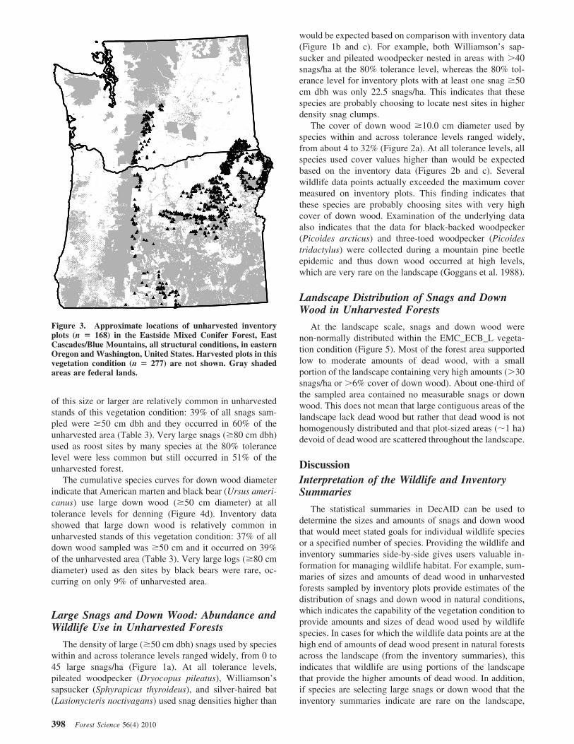
The Eastside Mixed Conifer Forest wildlife habitat typeis described in detail in Chappell et al. (2001). Locations ofinventory plots in the East Cascades and Blue Mountainssubregion of this wildlife habitat type are shown in DecAIDand in Figure 3. Stands in the larger tree structural conditionhave an average tree dbh �50.0 cm and tree stocking orcover �10%, and often are late-successional. Very large

Figure 1. Integrated summary of tolerance levels for Eastside Mixed Conifer Forest, East Cascades/BlueMountains, Larger Trees vegetation condition. (a) Wildlife species use of density of snags >50 cm dbh fornesting and roosting (includes data from North Cascades/Rockies and Smaller Trees). (b) Densities of snags>50 cm dbh and >2.0 m tall sampled on 95 unharvested inventory plots with snags present. (c) Densitiesof snags >50 cm dbh and >2.0 m tall on 159 unharvested inventory plots with and without snags present.In the upper box, the values 8.7, 13.1, and 22.5 are the 30, 50, and 80% tolerance limits, and 1.0 and 55.8are the minimum and maximum observed values. AMMA, American marten; BBWO, black-backedwoodpecker; PIWO, pileated woodpecker; PYNU, pygmy nuthatch (Sitta pygmaea); SHBA, silver-hairedbat; WISA, Williamson’s sapsucker; WHWO, white-headed woodpecker (Picoides albolarvatus).


trees may be scattered throughout the stand, a grass-forb orshrub understory is often present, and stands may or maynot have distinct canopy layers. Based on the inventorysample, 75% of the area of EMC_ECB_L is on federal landsand 64% has never been harvested in the past, and 77% ofthe unharvested area is federally owned.

Available Wildlife and Inventory Data

Wildlife data were not stratified by geographic subregionin this wildlife habitat type because few wildlife studieswere available, and habitat conditions in the subregions aresimilar. Data on wildlife use of snags at nesting, roosting,denning, and foraging sites were available for 26 speciesand three species groups from 31 studies for snag dbh(Figure 4a) and on 10 species and one species group from11 studies for snag density (Figure 1a). Data on wildlife(including ants) use of down wood size at foraging, den-ning, resting, or occupied sites were available for fourspecies and three groups from four studies for down wooddiameter (Figure 4c), and for three species and one group(fungi) from three studies for down wood cover (Figure 2a).Studies were primarily from eastern Oregon and Washing-ton; however, because data were limited, we included datafrom adjacent areas (British Columbia and western Mon-tana) where studies were from habitats similar to those in

Oregon and Washington. An annotated bibliography of allwildlife studies used in DecAID is found on the DecAIDwebsite.

Snags were sampled on 277 inventory plots in theEMC_ECB_L vegetation condition, 168 of which wereunharvested plots. Down wood data were collected on 273plots, 166 of which were unharvested. Snags were sampledon all ownerships, whereas down wood was sampled onlyon federal lands in Oregon but on all ownerships in Wash-ington. Tolerance levels for unharvested forests were cal-culated using 159 plots on federal lands (e.g., lower boxplots in Figures 1b and 2b). We also calculated tolerancelevels using just those plots (n � 95) on which at least onepiece of dead wood was tallied (e.g., upper box plots inFigures 1b and 2b). Inventory estimates discussed here arebased on plots with at least some dead wood present,because wildlife data were collected primarily on plotswhere they were associated with a piece of dead wood.

Snag and Down Wood Sizes: Abundance andWildlife Use in Unharvested Forests

In EMC_ECB_L, cumulative species curves for snag dbhindicate that most species use large snags �50 cm dbh at the50 and 80% tolerance levels for nesting, roosting, andforaging (Figure 4a–c). Inventory data indicated that snags

Figure 2. Integrated summary of tolerance levels for Eastside Mixed Conifer Forest, East Cascades/BlueMountains, Larger Trees vegetation condition. (a) Wildlife species use of cover of down wood > 10.0 cmdiameter for nesting and occupied sites (includes data from North Cascades/Rockies and Smaller Trees).(b) Cover of down wood >12.5 cm diameter sampled on 81 unharvested inventory plots with down woodpresent. (c) Cover of down wood >12.5 cm diameter sampled on 159 unharvested inventory plots with andwithout down wood present. See the legend to Figure 1 for explanation of the box plots. BBWO,black-backed woodpecker; PIWO, pileated woodpecker; TTWO, three-toed woodpecker; FUNGI, variousspecies of ectomycorrhizae and hypogeous fungi.


of this size or larger are relatively common in unharvestedstands of this vegetation condition: 39% of all snags sam-pled were �50 cm dbh and they occurred in 60% of theunharvested area (Table 3). Very large snags (�80 cm dbh)used as roost sites by many species at the 80% tolerancelevel were less common but still occurred in 51% of theunharvested forest.

The cumulative species curves for down wood diameterindicate that American marten and black bear (Ursus ameri-canus) use large down wood (�50 cm diameter) at alltolerance levels for denning (Figure 4d). Inventory datashowed that large down wood is relatively common inunharvested stands of this vegetation condition: 37% of alldown wood sampled was �50 cm and it occurred on 39%of the unharvested area (Table 3). Very large logs (�80 cmdiameter) used as den sites by black bears were rare, oc-curring on only 9% of unharvested area.

Large Snags and Down Wood: Abundance andWildlife Use in Unharvested Forests

The density of large (�50 cm dbh) snags used by specieswithin and across tolerance levels ranged widely, from 0 to45 large snags/ha (Figure 1a). At all tolerance levels,pileated woodpecker (Dryocopus pileatus), Williamson’ssapsucker (Sphyrapicus thyroideus), and silver-haired bat(Lasionycteris noctivagans) used snag densities higher than

would be expected based on comparison with inventory data(Figure 1b and c). For example, both Williamson’s sap-sucker and pileated woodpecker nested in areas with �40snags/ha at the 80% tolerance level, whereas the 80% tol-erance level for inventory plots with at least one snag �50cm dbh was only 22.5 snags/ha. This indicates that thesespecies are probably choosing to locate nest sites in higherdensity snag clumps.

The cover of down wood �10.0 cm diameter used byspecies within and across tolerance levels ranged widely,from about 4 to 32% (Figure 2a). At all tolerance levels, allspecies used cover values higher than would be expectedbased on the inventory data (Figures 2b and c). Severalwildlife data points actually exceeded the maximum covermeasured on inventory plots. This finding indicates thatthese species are probably choosing sites with very highcover of down wood. Examination of the underlying dataalso indicates that the data for black-backed woodpecker(Picoides arcticus) and three-toed woodpecker (Picoidestridactylus) were collected during a mountain pine beetleepidemic and thus down wood occurred at high levels,which are very rare on the landscape (Goggans et al. 1988).

Landscape Distribution of Snags and DownWood in Unharvested Forests

At the landscape scale, snags and down wood werenon-normally distributed within the EMC_ECB_L vegeta-tion condition (Figure 5). Most of the forest area supportedlow to moderate amounts of dead wood, with a smallportion of the landscape containing very high amounts (�30snags/ha or �6% cover of down wood). About one-third ofthe sampled area contained no measurable snags or downwood. This does not mean that large contiguous areas of thelandscape lack dead wood but rather that dead wood is nothomogenously distributed and that plot-sized areas (�1 ha)devoid of dead wood are scattered throughout the landscape.

DiscussionInterpretation of the Wildlife and InventorySummaries

The statistical summaries in DecAID can be used todetermine the sizes and amounts of snags and down woodthat would meet stated goals for individual wildlife speciesor a specified number of species. Providing the wildlife andinventory summaries side-by-side gives users valuable in-formation for managing wildlife habitat. For example, sum-maries of sizes and amounts of dead wood in unharvestedforests sampled by inventory plots provide estimates of thedistribution of snags and down wood in natural conditions,which indicates the capability of the vegetation condition toprovide amounts and sizes of dead wood used by wildlifespecies. In cases for which the wildlife data points are at thehigh end of amounts of dead wood present in natural forestsacross the landscape (from the inventory summaries), thisindicates that wildlife are using portions of the landscapethat provide the higher amounts of dead wood. In addition,if species are selecting large snags or down wood that theinventory summaries indicate are rare on the landscape,

Figure 3. Approximate locations of unharvested inventoryplots (n � 168) in the Eastside Mixed Conifer Forest, EastCascades/Blue Mountains, all structural conditions, in easternOregon and Washington, United States. Harvested plots in thisvegetation condition (n � 277) are not shown. Gray shadedareas are federal lands.


these structures can become an important focus formanagers.

For both snags and down wood, the inventory estimatesoften were lower than estimates from wildlife studies. Wethink this occurs primarily because the latter typically de-

scribe dead wood around nest, roost, denning, or foragingsites, where dead wood may be substantially more abundantthan in the surrounding area. Some wildlife species selectnest sites within clumps of snags. For example, pileatedwoodpecker, Williamson’s sapsucker, and silver-haired bat

Figure 4. Cumulative species curves of tol-erance levels for wildlife species use of sizesof dead wood in Eastside Mixed Conifer For-est, Larger Trees vegetation condition. Snagsizes used for (a) nesting, (b) denning orroosting, and (c) foraging; and (d) down woodsizes used at denning, resting, foraging, andoccupied sites. AMMA, American marten;BBBA, big brown bat; BBWO, black-backedwoodpecker; BCCH, black-capped chickadee(Parus atricapillus); BLBE, black bear;BRCR, brown creeper (Certhia americana);CAMY, California myotis (Myotis californi-cus); DEMO, deer mouse (Peromyscus man-iculatus); FLOW, flammulated owl (Otusflammeolus); GOEY, goldeneye (Bucephalaspp.); HAWO, hairy woodpecker (Picoidesvillosus); LANT, carpenter and formica ants(Camponotus spp. and Formica spp.); LEMY,long-eared myotis (Myotis evotis); LLMY,long-legged myotis (Myotis volans); MOCH,mountain chickadee (Parus gambeli); NFSQ,northern flying squirrel (Glaucomys sabri-nus); NOFL, northern flicker (Colaptes aura-tus); NPOW, northern pygmy-owl (Glau-cidium gnoma); NUCH, various species ofnuthatches and chickadees; PCE, variousspecies of primary cavity excavators; PIWO,pileated woodpecker; PYNU, pygmy nut-hatch; RBNU, red-breasted nuthatch (Sittacanadensis); RNSA, red-naped sapsucker(Sphyrapicus nuchalis); SANT, small ants(various species); SHBA, silver-haired bat;TTWO, three-toed woodpecker; SQUIR, var-ious species of squirrels; SRBV, southernred-backed vole (Clethrionomys gapperi);VASW, Vaux’s swift; WBNU, white-breastednuthatch (Sitta carolinensis); WHWO, white-headed woodpecker; WISA, Williamson’s sap-sucker; WOPE, woodpeckers (various species).


have tolerance levels above corresponding inventory toler-ance levels for large snags (Figure 1). Wildlife selection ofsnag and down wood clumps should be taken into consid-eration when dead wood habitat is managed.

In addition, the inventory estimates of down wood covermay be lower than the wildlife data values because mostwildlife studies included decay class 5 down wood, whichoften is the most abundant class (Spies et al. 1988), whereasthe inventories did not consistently include decay class 5(Ohmann and Waddell 2002). Also, the minimum diameterof down wood measured on inventory plots was 12.5 cm butfor most wildlife studies was 10 cm.

Sources of Variation in the Wildlife Data

High variance among wildlife use studies can result inwide tolerance intervals (e.g., the pileated woodpeckerpoints for large snag density, Figure 1a). Sources of vari-ability include differences among studies in methodology,plot size, and size and decay class breaks. Authors did notalways report complete information on how measurementswere taken. Where provided, we included these explana-tions in DecAID. Variability in the data also may arise fromvariation among individuals in a wildlife population andfrom variations in habitat conditions across study sites or

Figure 5. Relative frequency distribution of snags and down wood on unharvested inventory plots inEastside Mixed Conifer Forest, East Cascades/Blue Mountains, Larger Trees vegetation condition. (a)Density of snags >50 cm dbh and >2.0 m tall (n � 168). (b) Cover of down wood >12.5 cm diameter (n �166).

Table 3. Distribution of snags >25.4 cm dbh and >2.0 m tall and down wood >12.5 cm large end diameter among size classes inunharvested forest in the Eastside Mixed Conifer Forest, East Cascades/Blue Mountains, Larger Trees vegetation condition, basedon unharvested inventory plots

Size class(cm) % of all snags

% of area withsnags in size

class% of all

down wood% of area with

down wood in size class

12.5–25.3 — — 15 3525.4–49.9 60 60 48 5550.0–79.9 29 60 32 39�80.0 10 51 5 9

n � 168 for snags, n � 166 for down wood.


across entire research studies over both space and time. Thevarious sources of variability may result in outlier values,particularly in the cumulative species curves for 30 and 80%tolerance intervals. Published studies do not provide suffi-cient data to partition out the relative contributions of eachsource of variability nor to calculate propagation of erroracross multiple sources. However, any potential bias in oursummaries is probably reduced with greater numbers andextent of studies within a vegetation condition. We provideunderlying data from all individual studies in DecAID andencourage the user to become familiar with them and po-tential sources of bias.

Sampling and Scale Considerations inInterpreting the DecAID Summaries

The characterizations of dead wood populations must beinterpreted in light of the inherent spatial scale (grain andextent) imposed by the inventory and plot designs. Individ-ual observations (plots) consist of a sample of dead woodover approximately 1 ha. The distribution and estimatedvariation of dead wood across a sample of plots in a vege-tation condition is a function of the interaction of plot sizewith the abundance and spatial pattern of dead wood in thelandscape. For example, smaller plot sizes (or shortertransects) yield estimates with greater variation, becausesmaller plots are more likely to sample within dense clumpsof dead wood or within gaps with no wood. Because theplots sample an area that is smaller than a typical foreststand, the plot-level observations should not be viewed asrepresenting stand-level conditions. Rather, the summariesdescribe the aggregate properties and variability of deadwood on multiple 1-ha plots that sample a given vegetationcondition across a large landscape or region.

Wildlife data summarized in DecAID can be applied tomanagement and planning decisions at a range of spatialscales and geographic extents. Although the calculatedwildlife tolerance levels can be applied to stand-level man-agement decisions, it usually is not appropriate to apply onevalue (a particular tolerance level) to every stand across alandscape because stands vary in history, composition, dy-namics, and environmental setting. Instead, decisions ondistributing different levels of dead wood across a landscapecan be guided by the relative frequency distribution infor-mation from unharvested plots (Figure 5).

Tolerance levels and distributions summarized from in-ventory data also can be applied at multiple scales. As ageneral rule, we recommend geographic extents of nosmaller than approximately 50 km2 in size, which is thesmall end of the range of sizes typical of watersheds in ourregions at the level of fifth-field hydrologic unit codes. Thewildlife and inventory summaries also are appropriatelyapplied to very broad planning areas, such as for regionalassessments or National Forest planning. The maximumsize planning area to which the DecAID summaries areappropriately applied is limited only by the geographicdistribution of the wildlife studies and inventory plots usedin the summaries, in most cases all of Oregon andWashington.

Spatial Distribution of Dead Wood in theLandscape

Unfortunately, the inventory data and wildlife studies donot contain information on the spatial distribution of deadwood at local (plot or stand) nor landscape scales. However,if the primary objective is to manage for natural vegetationconditions rather than focusing on wildlife species, oneapproach is to mimic the distribution of unharvested area indifferent snag density and down wood cover classes (Figure5) across a landscape or watershed as a reference or guide.Although wildlife studies indicate that species often useclumps of snags and down wood, for most forest types thereis little specific guidance in the literature on the inherentspatial distribution of dead wood nor on the number or sizeof dead wood clumps used by wildlife that could guidemanagement.

Unharvested Plots as an Approximation ofNatural Conditions

Current dead wood on a site is strongly influenced bydisturbance and by the wood inherited from the precedingstand. Unfortunately, information on the disturbance historyof the plots was limited. Plots in unharvested, unroadedforest, which we used in DecAID to characterize naturalconditions, have been influenced to varying degrees by firesuppression, exotic pathogens, and other anthropogenic fac-tors. Because of decades of fire exclusion, areas with ahistorical disturbance regime of frequent fires may havemissed several fire cycles, often resulting in ingrowth ofsmaller trees of more shade-tolerant species. Suppression(self-thinning) mortality and increased insect and disease inthese denser stands may have increased density of smallersnags but not necessarily larger snags (Korol et al. 2002).However, information on historic amounts of dead woodavailable from other sources (Agee 2002, Korol et al. 2002,Brown et al. 2003) are similar to the amounts on theunharvested inventory plots (Mellen-McLean 2006).

Limitations of the DecAID Approach forGuiding Dead Wood Management

Although based on imperfect data, DecAID representsthe best data available on snags and down wood. Cautionsand limitations associated with the underlying data arethoroughly documented in DecAID (Mellen-McLean et al.2009) and need to be referenced by users when DecAID isapplied to projects. Used properly, DecAID can help guidemanagement of dead wood to meet management goals. Weassume that the meta-analysis approach of DecAID, com-bining data from across multiple studies and providing acomparison to forest inventory data, strengthens the evi-dence over applying data from individual studies.

DecAID provides a static picture of relationships be-tween wildlife and dead wood and of dead wood conditionsacross the current landscape. The dynamics of dead woodover time is an important consideration in managing wild-life habitat. Forest managers will need to use additionalanalytical tools to address temporal considerations, such as


the fire and fuels extension to the Forest Vegetation Simu-lator (Reinhardt and Crookston 2003). A summary of avail-able information on dead wood dynamics is provided on theDecAID website (Mellen-McLean et al. 2009).

The ultimate and really the only authentic measure of theeffectiveness of snag and down wood management guide-lines is how well they provide for fit individuals and viablepopulations. Few, if any, studies we reviewed truly mea-sured fitness and viability, and most studies did not reportdemographics (population density and trend) in relation todead wood habitat. Because of the difficulty and expense,we are unlikely to ever have rigorous, controlled, replicatedexperiments designed specifically to address this question.Lacking this, it is our fundamental assumption that patternsof species use and selection of dead wood size and amountsrepresent behaviors that have adaptive advantage for thespecies and that serve to bolster individual fitness. Thisassumption underlies our suggesting the use of the cumu-lative species curves to help guide dead wood management,even if they are based on post hoc observational studies inselected sites and not necessarily on more rigorously con-trolled manipulative experiments.

Applications to Forest Management

In the Pacific Northwest, DecAID currently is being usedto assess wildlife habitat contributions of dead wood fortimber sales, including salvage after wildfire, and otherforest management projects and regional assessments, in-cluding forest plan revisions. The Pacific Northwest Regionof the US Forest Service has developed a detailed guide tothe interpretation and use of the DecAID Advisor (USForest Service 2009) to provide suggestions and examplesof how to use the data in DecAID to assess impacts ofprojects on dead wood and dependent species.

Conclusions

Tolerance intervals are appropriate for describing pro-portions of observed (sampled) populations and aid in view-ing the data probabilistically and using it in risk manage-ment. We think tolerance intervals, corrected as necessaryfor small sample size, non-normal distributions, and differ-ing sampling intensities, are more meaningful and appro-priate than confidence or prediction intervals for represent-ing percentages of observed populations of wildlife use andinventories of dead wood.

Moreover, we have presented details of our methods ofcombining information across studies because others mayfind value in the same approach for a wide variety of otherforest management issues that pertain to questions such ashow much habitat is enough to provide for particular species(e.g., Kautz et al. 2006) or land area for biodiversity con-servation (e.g., Brashares and Sam 2005, Chen et al. 2006),Our approach can complement other methods of identifyingmanagement thresholds such as use of individual-baseddispersal models and area-optimization models, and pro-vides a new way to answer otherwise intractable questionswith empirical data.

Tear et al. (2005) called for scientific rigor in defining

quantitative objectives in conservation. Our method is rig-orous but flexible in that it allows managers to view out-comes at multiple tolerance levels. Results also can be usedboth ways, such as discerning the proportion of a naturalentity (e.g., a snag-using wildlife population) that could beprovided by a particular condition (e.g., a particular densityof snags of a given size), or, alternatively, what condition(snag density) would be needed to provide for a desirednatural condition (population level). In this way, our ap-proach could be generalized into a means of statisticallydefining thresholds for managing ranges of natural variationof forest ecosystems and communities (e.g., Cyr et al.2009).

Our approach entails combining available inventoriesand studies to furnish managers with a repeatable, rigorousbasis for decisionmaking. However, the degree of confi-dence, statistical tolerance, and proportion of a population,community, or natural system that is to be conserved ulti-mately is a matter of ownership goals and public policy,which, at best, would be informed by statistically soundanalyses as provided by our method.

Literature CitedAGEE, J.K. 2002. Fire as a coarse filter for snags and logs. P.

359–368 in Proc. of the Symposium on the ecology and man-agement of dead wood in western forests, Laudenslayer, W.F.,Jr., P.J. Shea, B.E. Valentine, C.P. Weatherspoon, and T.E.Lisle (eds.). US For. Serv. Gen. Tech. Rep. PSW-GTR-181.

BENDER, L.C., G.J. ROLOFF, AND J.B. HAUFLER. 1996. Evaluatingconfidence intervals for habitat suitability models. Wildl. Soc.Bull. 24(2):347–352.

BRASHARES, J.S., AND M.K. SAM. 2005. How much is enough?Estimating the minimum sampling required for effective mon-itoring of African reserves. Biodiv. Conserv. 14:2709–2722.

BROWN, J.K., E.D. REINHARDT, AND K.A. KRAMER. 2003. Coarsewoody debris: Managing benefits and fire hazard in the recov-ering forest. US For. Serv. Gen. Tech. Rep. RMRS-GTR-105.16 p.

BULL, E.L., T.W. HEATER, AND J.F. SHEPARD. 2005. Habitatselection by the American marten in northeastern Oregon.Northw. Sci. 79(1):37–43.

BULL, E.L., AND J.E. HOHMANN. 1993. The association betweenVaux’s swifts and old growth forests in northeastern Oregon.West. Birds 24:38–42.

BULL, E.L., C.G. PARKS, AND T.R. TORGERSEN. 1997. Trees andlogs important to wildlife in the interior Columbia River basin.US For. Serv. Gen. Tech. Rep. PNW-GTR-391. 55 p.

CHAPPELL, C.B., R.C. CRAWFORD, C. BARRETT, J. KAGAN, D.H.JOHNSON, M. O’MEALY, G.A. GREEN, H.L. FERGUSON, W.D.EDGE, E.L. GREDA, AND T.A. O’NEIL. 2001. Wildlife habitats:Descriptions, status, trends, and system dynamics. P. 22–114 inWildlife-habitat relationships in Oregon and Washington,Johnson, D.H., and T.A. O’Neil (eds.). Oregon State UniversityPress, Corvallis, OR.

CHEN, X., B.A. LI, T. SCOTT, AND M.F. ALLEN. 2006. Toleranceanalysis of habitat loss for multispecies conservation in westernRiverside County, California, USA. Int. J. Biodiv. Sci. Manag.2(2):87–96.

CHERRY, S. 1996. A comparison of confidence interval methodsfor habitat use-availability studies. J. Wildl. Manag.60(3):653–658.

CYR, D., S. GAUTHIER, Y. BERGERON, AND C. CARCAILLET. 2009.Forest management is driving the eastern North American


boreal forest outside its natural range of variability. Front.Ecol. Environ. 7(10):519–524.

DOMINICI, F., G. PARMIGIANI, R. WOLPERT, AND K. RECKHOW.1997. Combining information from related regressions. J. Ag-ric. Biol. Environ. Statist. 2(3):313–332.

DRAPER, D., D.P. GAVER, JR., P.K. GOEL, J.B. GREENHOUSE, L.V.HEDGES, C.N. MORRIS, J.R. TUCKER, AND C.M. WATERNAUX.1992. Combining information. Statistical issues and opportu-nities for research. Contemporary Statistics No. 1. NationalAcademy Press, Washington, DC, 217 p.

GOGGANS, R., R.D. DIXON, AND L.C. SEMINARA. 1988. Habitatuse by three-toed and black-backed woodpeckers, DeschutesNational Forest, Oregon. Nongame Rpt. 87-3-02. OregonDept. Fish and Wildlife and Deschutes National Forest. 49 p.

GUIDA, M., AND F. PENTA. 2010. A Bayesian analysis of fatiguedata. Struct. Saf. 32:64–76.

GUREVITCH, J., AND L.V. HEDGES. 1999. Statistical issues in eco-logical meta-analyses. Ecology 80(4):1142–1149.

HAHN, G.J., AND W.Q. MEEKER. 1991. Statistical intervals: Aguide for practitioners. John Wiley & Sons, New York, NY.392 p.

KAUTZ, R., R. KAWULA, T. HOCTOR, J. COMISKEY, D. JANSEN, D.JENNINGS, J. KASBOHM, F. MAZZOTTI, R. MCBRIDE, AND L.RICHARDSON. 2006. How much is enough? Landscape-scaleconservation for the Florida panther. Bio. Conserv.130(1):118–133.

KOROL, J.J., M.A. HEMSTROM, W.J. HANN, AND R. GRAVENMIER.2002. Snags and down wood in the Interior Columbia BasinEcosystem Management Project. P. 649–663 in Proc. of theSymposium on the ecology and management of dead wood inwestern forests. Laudenslayer, W.F. Jr., P.J. Shea, B.E. Valen-tine, C.P. Weatherspoon, and T.E. Lisle (eds.). US For. Serv.Gen. Tech. Rep. PSW-GTR-181.

KRISHNAMOORTHY, K. 2001. StatCalc. Available from http://www.ucs.louisiana.edu/�kxk4695/StatCalc.htm; last accessedJan. 20, 2010.

KRISHNAMOORTHY, K. 2006. Handbook of statistical distributionswith applications. Chapman & Hall/CRC, Boca Raton, FL.376 p.

KRISHNAMOORTHY, K., AND T. MATHEW. 2009. Statistical toler-ance regions: Theory, applications and computation. JohnWiley & Sons, New York, NY. 461 p.

LUNDQUIST, R.W., AND J.M. MIRIANI. 1991. Nesting habitat andabundance of snag-dependent birds in the southern WashingtonCascade Range. P. 221–240 in Wildlife and vegetation ofunmanaged Douglas-fir forests, Ruggiero, L.F., K.B. Aubry,A.B. Carey, and M. Huff (eds.). US For. Serv. Gen. Tech. Rep.PNW-GTR-285.

MARCOT, B.G. 1992. Snag recruitment simulator, Rel. 3.1. USFor. Serv. Pacific Northwest Region, Portland OR.

MARCOT, B.G., K. MELLEN, S.A. LIVINGSTON, AND C. OGDEN.2002. The DecAID advisory model: Wildlife component. P.561–590 in Proc. of the Symposium on the ecology and man-agement of dead wood in western forests, Laudenslayer, W.F.,Jr., P.J. Shea, B.E. Valentine, C.P. Weatherspoon, and T.E.Lisle (eds.). US For. Serv. Gen. Tech. Rep. PSW-GTR-181.

MCCOMB, B., K. MCGARIGAL, S. HOPE, AND M. HUNTER. 1992.Monitoring cavity-nesting bird use in clearcuts and watershedson western Oregon National Forests. Progress report. Dept. ofForest Science, Oregon State University, Corvallis, OR. 48 p.

MCCOMB, W.C., M.T. MCGRATH, T.A. SPIES, AND D. VESELY.2002. Models for mapping potential habitat at landscape scales:An example using northern spotted owls. For. Sci. 48:203–216.

MELLEN, K., B.G. MARCOT, J.L. OHMANN, K.L. WADDELL, E.A.WILLHITE, B.B. HOSTETLER, S.A. LIVINGSTON, AND C. OGDEN.

2002. DecAID: A decaying wood advisory model for Oregonand Washington. P. 527–533 in Proc. of the Symposium on theecology and management of dead wood in western forests,Laudenslayer, W.F., Jr., P.J. Shea, B.E. Valentine, C.P. Weath-erspoon, and T.E. Lisle (eds.). US For. Serv. Gen. Tech. Rep.PSW-GTR-181.

MELLEN-MCLEAN, K. 2006. Comparison of historical range ofvariability for dead wood: DecAID vs. other published esti-mates. DecAID Implementation Guide. Available online at www.fs.fed.us/r6/nr/wildlife/decaid-guide/hrv-dead-wood-comparison.shtml; last accessed Jan. 20, 2010.

MELLEN-MCLEAN, K., B.G. MARCOT, J.L. OHMANN, K. WADDELL,S.A. LIVINGSTON, E.A. WILLHITE, B.B. HOSTETLER, C. OGDEN,AND T. DREISBACH. 2009. DecAID, the decayed wood advisorfor managing snags, partially dead trees, and down wood forbiodiversity in forests of Washington and Oregon. Version 2.1.Available online at www.fs.fed.us/r6/nr/wildlife/decaid/index.shtml; last accessed Jan. 20, 2010.

MOOD, A.M., F.A. GRAYBILL, AND D.C. BOES. 1974. Introductionto the theory of statistics. McGraw-Hill, New York, NY. 564 p.

NEITRO, W.A., V.W. BINKLEY, S.P. CLINE, R.W. MANNAN, B.G.MARCOT, D. TAYLOR, AND F.F. WAGNER. 1985. Snags (wildlifetrees). P. 129–169 in Management of wildlife and fish habitatsin forests of western Oregon and Washington. Part 1—Chapternarratives, Brown, E.R. (ed.). US For. Serv., Portland, OR.

NIGH, G. 1998. Prediction intervals for estimates of site indexbased on ecosystem type. Environ. Manag. 22:197–202.

OHMANN, J.L., AND K.L. WADDELL. 2002. Regional patterns ofdead wood in forested habitats of Oregon and Washington. P.535–560 in Proc. of the Symposium on the ecology and man-agement of dead wood in western forests, Laudenslayer, W.F.,Jr., P.J. Shea, B.E. Valentine, C.P. Weatherspoon, and T.E.Lisle (eds.). US For. Serv. Gen. Tech. Rep. PSW-GTR-181.

O’NEIL, T.A., K.A. BETTINGER, M. VANDER HEYDEN, B.G. MAR-COT, C. BARRETT, T.K. MELLEN, W.M. VANDER HAEGEN, D.H.JOHNSON, P.J. DORAN, L. WUNDER, AND K.M. BOULA. 2001a.Structural conditions and habitat elements of Oregon andWashington. P. 115–139 in Wildlife–habitat relationships inOregon and Washington, Johnson, D.H., and T.A. O’Neil(eds.). Oregon State University Press, Corvallis, OR.

O’NEIL, T.A., D.H. JOHNSON, C. BARRETT, M. TREVITHICK, K.A.BETTINGER, C. KIILSGARRD, M. VANDER HEYDEN, E.L. GREDA,D. STINSON, B.G. MARCOT, P.J. DORAN, S. TANK, AND L.WUNDER. 2001b. Matrixes for wildlife–habitat relationships inOregon and Washington. In Wildlife–habitat relationships inOregon and Washington, Johnson, D.H., and T.A. O’Neil, T.A.(eds.). Oregon State University Press, Corvallis, OR.

ORMSBEE, P.C., AND W.C. MCCOMB. 1998. Selection of day roostsby female long-legged myotis in the central Oregon CascadeRange. J. Wildl. Manag. 62(2):596–603.

PENA, D. 1997. Combining information in statistical modeling.Am. Statist. 51(4):326–332.

REINHARDT, E.D., AND N.L. CROOKSTON. 2003. The fire and fuelsextension to the forest vegetation simulator. US For. Serv. Gen.Tech. Rep. RMRS-GTR-116.

ROSE, C.L., B.G. MARCOT, T.K. MELLEN, J.L. OHMANN, K.L.WADDELL, D.L. LINDLEY, AND B. SCHREIBER. 2001. Decayingwood in Pacific Northwest forests: Concepts and tools forhabitat management. P. 580–623 in Wildlife-habitat relation-ships in Oregon and Washington, Johnson, D.H., and T.A.O’Neil (eds.). Oregon State University Press, Corvallis, OR.

SCHREIBER, B.P. 1987. Diurnal bird use of snags on clearcuts incentral coastal Oregon. M.Sc. Thesis, Oregon State Univ.,Corvallis, OR. 63 p.


SMITH, J.G., J.J. BEAUCHAMP, AND A.J. STEWART. 2005. Alterna-tive approach for establishing acceptable thresholds on macro-invertebrate community metrics. J. N. Am. Benth. Soc.24(2):428–440.

SPIES, T.A., J.F. FRANKLIN, AND T.B. THOMAS. 1988. Coarsewoody debris in Douglas-fir forests of western Oregon andWashington. Ecology 69:1689–1702.

STEIDL, R.J., J.P. HAYNES, AND E. SCHAUBER. 1997. Statisticalpower analysis in wildlife research. J. Wildl. Manag.61(2):270–279.

TEAR, T.H., P. KAREIVA, P.L. ANGERMEIER, P. COMER, B. CZECH,R. KAUTZ, L. LANDON, D. MEHLMAN, K. MURPHY, AND M.RUCKELSHAUS. 2005. How much is enough? The recurrentproblem of setting measurable objectives in conservation. Bio-Science 55(10):835–850.

THOMAS, J.W., R.G. ANDERSON, C. MASER, AND E.L. BULL. 1979.

Snags. P. 60–77 in Wildlife habitats in managed forests theBlue Mountains of Oregon and Washington, Thomas, J.W.(ed.). US Agricultural Handbook 553.

THOMAS, L. 1997. Retrospective power analysis. Cons. Bio.11(1):276–280.

US FOREST SERVICE. 2009. A Guide to the Interpretation and Useof the DecAID Adviser. Available online at www.fs.fed.us/r6/nr/wildlife/decaid-guide/index.shtml; last accessed Jan.20, 2010.

VONHOF, M.J., AND J.C. GWILLIAM. 2007. Intra- and interspecificpatterns of day roost selection by three species of forest-dwell-ing bats in Southern British Columbia. For. Ecol. Manag.252:165–175.

ZIELINSKI, W.J., R.L. TRUEX, G.A. SCHMIDT, F.V. SCHLEXER, K.N.SCHMIDT, AND R.H. BARRETT. 2004. Resting habitat selectionby fishers in California. J. Wildl. Manag. 68(3):475–492.


synthesis of regional wildlife and vegetation field ... · synthesis of regional wildlife and...

Documents