Proceedings of IEEE-RAS International Conference onHumanoid Robots (HUMANOIDS2001)

Tokyo, Japan, pp. 319–326, November 2001

Synthesis of a Walking Primitive Database for a Humanoid Robotusing Optimal Control Techniques

J. Denk and G. Schmidt

Institute of Automatic Control Engineering,Technische Universit¨at Munchen,

D-80290 Munich, GermanyJoachim.Denk@ei.tum.de, Guenther.Schmidt@ei.tum.de

AbstractThis paper presents a general method for generatingwalking primitives for anthropomorphic 3D–bipeds.Corresponding control torques allowing straight aheadwalking with pre–swing, swing, and heel–contact arederived by dynamic optimization using a direct collo-cation approach. The computed torques minimize anenergy based, mixed performance index. Zero momentpoint (ZMP) and friction conditions at the feet ensur-ing postural stability of the biped, as well as bounds onthe joint angles and on the control torques, are treatedas constraints. The method is applied to the model ofa biped with 12 joints for the purpose of developinga walking primitive database allowing straight aheadwalking with situation dependent step–length adapta-tion. The resulting biped motions are dynamically sta-ble and the overall motion behaviour is remarkablyclose to that of humans.

KeywordsHumanoid Robot, Optimal Control, Walking PrimitiveDatabase, Step–Length Adaptation.

1 IntroductionOver the last years, major progress has been made inconstruction and stabilization of biped walking ma-chines. Perception based goal–oriented autonomouswalking, however, still remains an open field of re-search [1]. Locomotion in a partly unknown environ-ment requires the ability of the biped to adapt its gaitpattern according to the present situation, so that ob-stacles in the walking trail can be passed by or over-come. But, unlike industrial robots, bipeds are notfixed rigidly to the ground and have the tendency totip over very easily. Their postural stability dependson the behaviour of six unpowered DOF defining theirpose in the world, which can only be influenced in-directly by appropriate actuation of the powered DOFin the joints. Usually, the problem of executing a sta-ble step–sequence is therefore solved by precomputa-tion of an adequate reference trajectory, i.e., a walk-

ing pattern. As a consequence of the high nonlinear-ity and complexity of the system, however, it is notpossible to achieve this in real time for a 3D biped ingeneral. A possible solution is to compute a series ofwalking primitives for steps with different step param-eters offline and to store them in a database. A situ-ation dependent walking pattern can then be obtainedby selection and concatenation of appropriate walkingprimitives during run–time.Often, the problem of walking primitive synthesis issimplified by prescribing time trajectories for selectedbody parts [2–4]. These trajectories depend on thecharacteristics of the actual biped robot. The taskof determining suitable trajectories relies on the de-signer’s intuition and / or observations and biometricmeasurements of human gait behaviour. A methodfor walking primitive synthesis without any prescrip-tion of a priori knownledge about the motion has beenreported in [5]. Dynamic optimization was appliedto the model of a human body in order to find a re-peatable movement minimizing metabolic energy permeter walked. The amount of supercomputer timeneeded, however, was excessive.This paper deals with a general approach, which issuited for synthesizing databases of dynamically sta-ble walking primitives [2] automatically in feasibletime, by fusing the advantages of the methods men-tioned earlier. To achieve this, first, the search spacefor a walking primitive is reduced by the general andreasonable assumption, that a walking primitive com-prises the three gait phases pre–swing, swing andheel–contact and that one foot always remains flaton the ground while the other one is moving. Ade-quate motions are parameterized by the step param-eters, i.e., step–length, step–width, and timing of thegait–phases. The search space is further confined tophysically admissible trajectories. These trajectoriessatisfy the zero moment point (ZMP) [3] and fric-tion conditions ensuring postural stability of the biped,conditions for smooth walking primitive concatena-tion and restrictions on joint angles and on the con-

319

trol torques given by the electrical and mechanical de-sign. The remaining set of primitives is then searchedfor the walking primitive minimizing an energy based,mixed performance index using dynamic optimization.The corresponding optimal control problem is solvednumerically by discretization of time using a direct–collocation approach [6]. Direct–collocation has al-ready been applied successfully to synthesize walkingprimitives for a planar biped [7]; other examples of en-ergy optimal planar walking are given in [8,9].The paper is structured as follows. The problem is for-mulated in Sec. 2 and the considered class of bipedwalking machines is defined. In Sec. 3 the searchspace for the optimization problem is characterizedmathematically by specifying the properties of a walk-ing primitive and the conditions for physical admis-sibility. After a discussion of the dynamic modellingapproach used in Sec. 4, the optimal control problemis summerized in Sec. 5. We applied our approach asan example to the model of an anthropomorphic 3D–biped with 12 joints. A walking primitive databasewas generated allowing straight ahead walking withthe step–lengths0:30 m,0:31 m, : : :, 0:50 m. The nec-essary procedure and corresponding numerical resultsare presented in Sec. 6.

2 Problem Formulation

Figure 1: Kinematic scheme of biped robot with headframeH .

The described method is applicable to walking ma-chines of the type illustrated in Fig. 1 consisting ofbodiesBi, i = 1 : : :Nb connected by driven jointswith the joint angles and control torquesqi and �i,

Figure 2: Biped feet with coordinate frames, lengthsl,and pointsr.

i = 1 : : :Nj respectively. Symmetry of the biped’sleft and right side is assumed. The legs have to com-prise at least six powered joints each, allowing to ma-nipulate the feet in 6 DOF in Cartesian space relativeto the torso. Further joints in the biped’s torso are notconsidered in this work, but could be regarded in prin-ciple. The feet of the biped are assumed to be of sucha kind, that the contact behaviour can be approximatedby rigid body contacts, see Fig. 2.As input to the problem, the biped’s kinematical pa-rameters, all necessary dimensions, the masses and in-ertia tensors of the bodiesBi, the restrictions on jointanglesqi and joint velocities_qi, the maximum allowedmotor torques and the coefficients of friction betweenthe feet and the ground have to be provided.The joint angles are then subsumed in the vectorq =

[ql; qr], with the vectorsql = [q1 : : : qNj=2]T and

qr = [qNj=2+1 : : : qNj]T representing the angles of

the left and right leg respectively. Four coordinate sys-tems are defined, the world coordinate systemO, thehead frameH and the contact framesL andR fixedin the sole of the left and right foot respectively. Thepose ofH , L andR with respect toO is given bypH = [rH ;�H ], pL = [rL;�L] andpR = [rR;�R].The elements of vectorr = [rx ry rz ]

T are Cartesiancoordinates,� = [�x �y �z ]

T are orientations repre-sented by roll–, pitch–, and yaw–angles. The postureof the biped is defined by the generalized coordinatesqg = [q;pL].The goal is now to synthesize a database of walkingprimitives allowing straight ahead walking with step–length adaptation. The individual primitives need to becomputed in such a way, that they can be concatenatedin realtime resulting in a smooth and physically fea-sible joint trajectory together with the correspondingcontrol torques needed for driving the biped.

3 Walking PrimitiveIn the following subsections the search space of the op-timal control problem is defined mathematically. First,the kinematics of a walking primitive are specified,

320

next, the conditions for contact stability are stated.Physical admissibility in addition requires that thejoint angle and joint torque trajectories conform withrestrictions given by the mechanical and electrical de-sign. This problem is discussed in Sec. 3.3. Finally,conditions allowing the concatenation of individualwalking primitives to a smooth trajectory are derivedin Sec. 3.4.

3.1 Walking Primitive Kinematics

rR

Lez =

Oez

rRb

Rez

Oez

Oez

Oex

Oex

Rex

PhaseHeel−Contact−

t 2 [t2; ts]

Swing−Phase

t 2 [t1; t2[

Phase

Rez

rL = O

Pre−Swing−

rRf

Rex

O

Rez

Rex

rRbO

Lex =

Oex

II)

I)

III)

t 2 [0; t1[

l1 l1 � lxf

l2 � lxb

l2

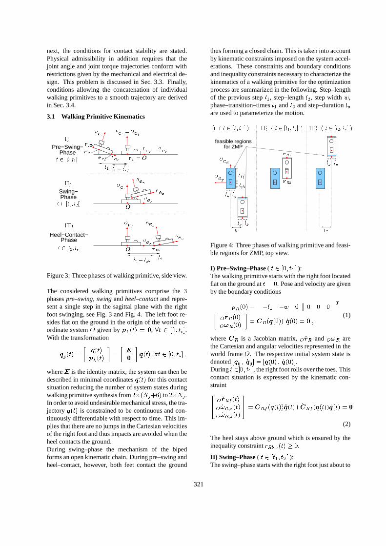
Figure 3: Three phases of walking primitive, side view.

The considered walking primitives comprise the 3phasespre–swing, swingandheel–contactand repre-sent a single step in the sagittal plane with the rightfoot swinging, see Fig. 3 and Fig. 4. The left foot re-sides flat on the ground in the origin of the world co-ordinate systemO given bypL(t) = 0, 8t 2 [0; ts].With the transformation

qg(t) =

�q(t)

pL(t)

�=

�E

0

�q(t) ;8t 2 [0; ts] ;

whereE is the identity matrix, the system can then bedescribed in minimal coordinatesq(t) for this contactsituation reducing the number of system states duringwalking primitive synthesis from2�(Nj+6) to2�Nj .In order to avoid undesirable mechanical stress, the tra-jectoryq(t) is constrained to be continuous and con-tinuously differentiable with respect to time. This im-plies that there are no jumps in the Cartesian velocitiesof the right foot and thus impacts are avoided when theheel contacts the ground.During swing–phase the mechanism of the bipedforms an open kinematic chain. During pre–swing andheel–contact, however, both feet contact the ground

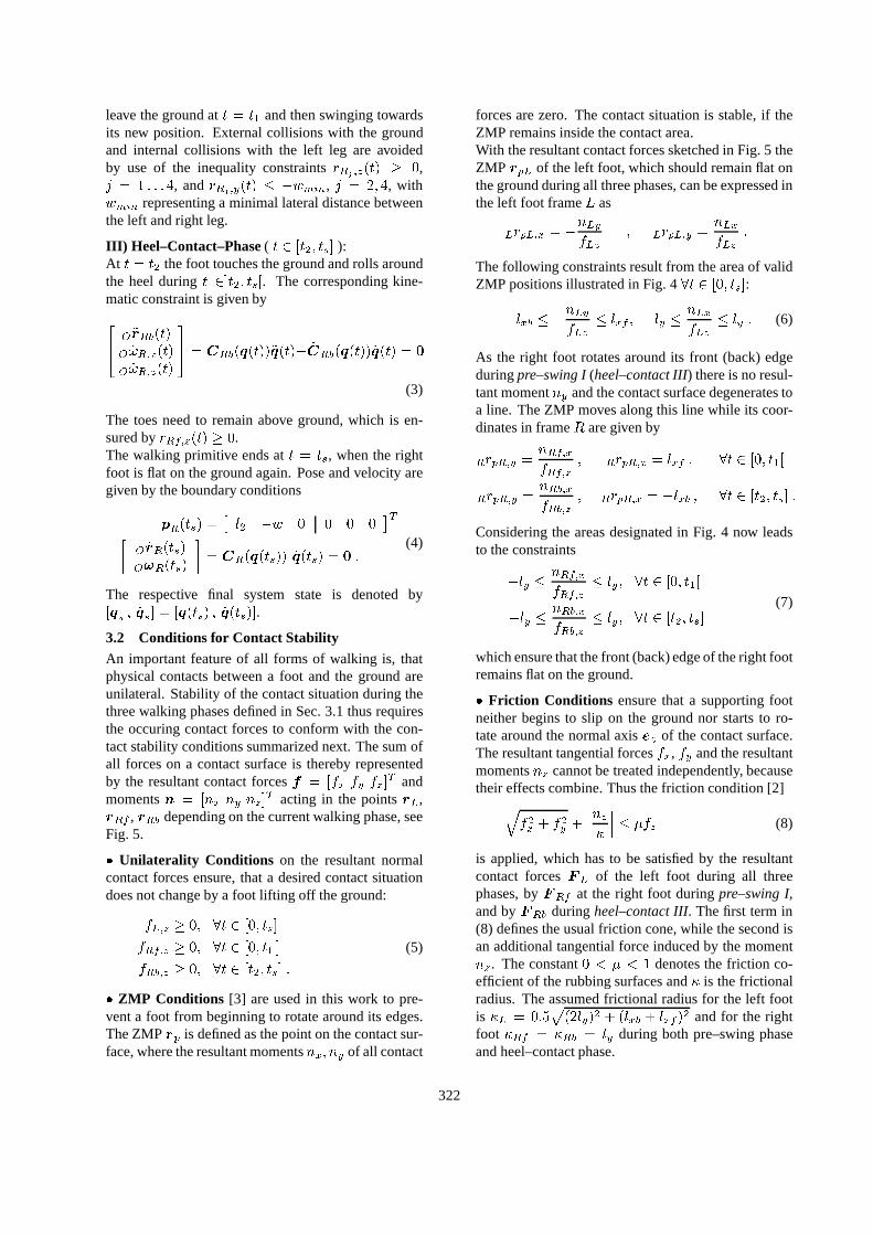
thus forming a closed chain. This is taken into accountby kinematic constraints imposed on the system accel-erations. These constraints and boundary conditionsand inequality constraints necessary to characterize thekinematics of a walking primitive for the optimizationprocess are summarized in the following. Step–lengthof the previous stepl1, step–lengthl2, step widthw,phase–transition–timest1 andt2 and step–durationtsare used to parameterize the motion.

lyly

Oey

ly

I) ( t 2 [0; t1[ ) II) ( t 2 [t1; t2[ )

rRb

rRf

lxb

lxf

ly ly

III) ( t 2 [t2; ts] )

for ZMP

Oex

w

ly

w

feasible regions

Figure 4: Three phases of walking primitive and feasi-ble regions for ZMP, top view.

I) Pre–Swing–Phase ( t 2 [0; t1[ ):The walking primitive starts with the right foot locatedflat on the ground att = 0. Pose and velocity are givenby the boundary conditions

pR(0) =��l1 �w 0 0 0 0

�T�

O _rR(0)

O!R(0)

�= CR(q(0)) _q(0) = 0 ;

(1)

whereCR is a Jacobian matrix,O _rR andO!R arethe Cartesian and angular velocities represented in theworld frameO. The respective initial system state isdenoted[q0 ; _q0] = [q(0) ; _q(0)].Duringt 2]0; t1[, the right foot rolls over the toes. Thiscontact situation is expressed by the kinematic con-straint

24 O�rRf (t)

O _!R;x(t)

O _!R;z(t)

35 = CRf (q(t))�q(t)+ _CRf (q(t)) _q(t) = 0

(2)

The heel stays above ground which is ensured by theinequality constraintrRb;z(t) � 0.

II) Swing–Phase ( t 2 [t1; t2[ ):The swing–phase starts with the right foot just about to

321

leave the ground att = t1 and then swinging towardsits new position. External collisions with the groundand internal collisions with the left leg are avoidedby use of the inequality constraintsrRj ;z(t) � 0,j = 1 : : : 4, andrRj ;y(t) � �wmin, j = 2; 4, withwmin representing a minimal lateral distance betweenthe left and right leg.

III) Heel–Contact–Phase ( t 2 [t2; ts] ):At t = t2 the foot touches the ground and rolls aroundthe heel duringt 2]t2; ts[. The corresponding kine-matic constraint is given by

24 O�rRb(t)

O _!R;x(t)

O _!R;z(t)

35 = CRb(q(t))�q(t)+ _CRb(q(t)) _q(t) = 0

(3)

The toes need to remain above ground, which is en-sured byrRf;z(t) � 0.The walking primitive ends att = ts, when the rightfoot is flat on the ground again. Pose and velocity aregiven by the boundary conditions

pR(ts) =�l2 �w 0 0 0 0

�T�

O _rR(ts)

O!R(ts)

�= CR(q(ts)) _q(ts) = 0 :

(4)

The respective final system state is denoted by[qs ; _qs] = [q(ts) ; _q(ts)].

3.2 Conditions for Contact StabilityAn important feature of all forms of walking is, thatphysical contacts between a foot and the ground areunilateral. Stability of the contact situation during thethree walking phases defined in Sec. 3.1 thus requiresthe occuring contact forces to conform with the con-tact stability conditions summarized next. The sum ofall forces on a contact surface is thereby representedby the resultant contact forcesf = [fx fy fz]

T andmomentsn = [nx ny nz]

T acting in the pointsrL,rRf , rRb depending on the current walking phase, seeFig. 5.

� Unilaterality Conditions on the resultant normalcontact forces ensure, that a desired contact situationdoes not change by a foot lifting off the ground:

fL;z � 0; 8t 2 [0; ts]

fRf;z � 0; 8t 2 [0; t1[

fRb;z � 0; 8t 2 [t2; ts] :

(5)

� ZMP Conditions [3] are used in this work to pre-vent a foot from beginning to rotate around its edges.The ZMPrp is defined as the point on the contact sur-face, where the resultant momentsnx; ny of all contact

forces are zero. The contact situation is stable, if theZMP remains inside the contact area.With the resultant contact forces sketched in Fig. 5 theZMP rpL of the left foot, which should remain flat onthe ground during all three phases, can be expressed inthe left foot frameL as

LrpL;x = �nLy

fLz

; LrpL;y =nLx

fLz

:

The following constraints result from the area of validZMP positions illustrated in Fig. 48t 2 [0; ts]:

�lxb � �nLy

fLz

� lxf ; �ly �nLx

fLz

� ly : (6)

As the right foot rotates around its front (back) edgeduringpre–swing I(heel–contact III) there is no resul-tant momentny and the contact surface degenerates toa line. The ZMP moves along this line while its coor-dinates in frameR are given by

RrpR;y =nRf;x

fRf;z

; RrpR;x = lxf ; 8t 2 [0; t1[

RrpR;y =nRb;x

fRb;z

; RrpR;x = �lxb ; 8t 2 [t2; ts] :

Considering the areas designated in Fig. 4 now leadsto the constraints

�ly �nRf;x

fRf;z

� ly; 8t 2 [0; t1[

�ly �nRb;x

fRb;z

� ly; 8t 2 [t2; ts](7)

which ensure that the front (back) edge of the right footremains flat on the ground.

� Friction Conditions ensure that a supporting footneither begins to slip on the ground nor starts to ro-tate around the normal axisez of the contact surface.The resultant tangential forcesfx, fy and the resultantmomentsnz cannot be treated independently, becausetheir effects combine. Thus the friction condition [2]

qf2x + f

2y +

���nz�

��� � �fz (8)

is applied, which has to be satisfied by the resultantcontact forcesFL of the left foot during all threephases, byFRf at the right foot duringpre–swing I,and byFRb duringheel–contact III. The first term in(8) defines the usual friction cone, while the second isan additional tangential force induced by the momentnz. The constant0 < � < 1 denotes the friction co-efficient of the rubbing surfaces and� is the frictionalradius. The assumed frictional radius for the left footis �L = 0:5

p(2ly)2 + (lxb + lxf )2 and for the right

foot �Rf = �Rb = ly during both pre–swing phaseand heel–contact phase.

322

right foot

III) ( t 2 [t2; ts] )

left foot

rRf

I), II), III) ( t 2 [0; ts] )

rRb

rRb

fL;y; nL;y rL

fL;z; nL;z

fL;x; nL;x

I) ( t 2 [0; t1[ )

rRf

fRf;y; nRf;y = 0fRf;x; nRf;x

fRf;z; nRf;zfRb;z; nRb;z

fRb;x; nRb;x

fRb;y; nRb;y = 0

Figure 5: Contact constraints and forces during phases of walking primitive.

3.3 Mechanical and Electrical RestrictionsPhysical admissibility of the walking primitives alsodemands compliance with restrictions given by theperformance limits of the motors and by the mechani-cal mechanism. This is regarded by the inequality con-straints

qmin � q(t) � qmax

_qmin � _q(t) � _qmax; 8t = [0; ts]:

�min � � (t) � �max

(9)

3.4 Conditions for Walking PrimitiveConcatenation

Step-length adaptation requires the concatenation ofcyclic and transition walking primitives. These primi-tives are specified by additional constraints on the ini-tial and final system states[q0; _q0] and [qs; _qs]. Forderivation of the related boundary conditions we willmake use of the symmetry in the kinematic structureof the biped, allowing to easily obtain a walking prim-itive for the right foot supporting the biped, denotedby ~q(t), from the walking primitiveq(t). It results byinterchanging the joint angles of the left and right leg,which is performed by the mapping

~q(t) = [qr(t); ql(t)] ; t = [0; ts] : (10)

Respective joint torques� (t) are mapped accordingly.In order to obtain a cyclic walking primitive, the addi-tional boundary conditions

qs = ~q0 and _qs =_~q0 (11)

are stated for a walking primitive withl1 = l2 = a.This allows the concatenation ofq and~q into a smoothwalking patternq, ~q, q, ~q, q, : : : enabling continuoussymmetric cyclic walking with a given step–lengtha,see also [1]. A cyclic walking primitive is denoted byql1;l2 = q

a;a in the following.For concatenation of two cyclic walking primitivesqa;a andqb;b with different step–lengthsa 6= b, see

Fig. 6, a transition walking primitiveqa;b is defined.In order to obtain a continuous state trajectory afterconcatenation, initial and final states of the transitionprimitive have to match the corresponding states of the

cyclic primitives. This is ensured by the boundary con-ditions

qa;b0 = ~qa;a

s and _qa;b0 = _~qa;a

s ;

qa;bs = ~qb;b

0 and _qa;bs = _~qb;b

0 :

(12)

When the transition primitive is mapped according to(10) the primitive~qa;b shown in the center of Fig. 6is obtained. This primitive can then be concatenatedwith the two cyclic primitives yielding the completetransition as depicted in Fig. 6 on the right. The result-ing walking pattern enables the biped to execute threesteps with the step–lengthsa, b andb.In order to enable walking withn different step–lengths, a database ofn cyclic walking primitives withdifferent step–lengthsl = l1 = l2 needs to be com-puted. Considering possible transitions between all ofthe cyclic primitivesp = n(n�1) transition primitivesare required.

4 Dynamic ModelingThe system dynamics in the three phases are modeledunder the assumption of bilateral rigid body contactsbetween the feet and the ground. This allows the exer-tion of contact forces in all directions contrary to phys-ical reality. In combination with the contact stabilityconditions formulated in Sec. 3.2, however, the model-ing is permissible, because they prevent the occurrenceof contact forces not being compatible with the actualunilateral contact situation.The dynamics of the biped in minimal coordinatesq(t) 2 IRNj are then given by

M �q = h+ � +CTRfFRf +C

TRbFRb (13)

with M(q) the mass–matrix,h(q; _q) coriolis, cen-trifugal, and gravity effects, and� the jointtorques. The JacobiansCRf (q) 2 IR5�Nj andCRb(q) 2 IR5�Nj obtained in (2) and (3) areprojecting the generalized constraint contact forcesFRb = [fRb; nRb;x; nRb;z] 2 IR5�1 and FRf =

[fRf ; nRf;x; nRf;z] 2 IR5�1 on the generalized co-ordinates. Since the contact situation of the left foot isformulated in minimal coordinates, the forcesFL =

[fL;nL] 2 IR6�1 are not part of the dynamic system

323

l1 = a

l1 = a

l1 = b

l2 = b

l2 = b

b

b

a

a

l2 = a

qa;a

qa;b

~qa;b

qb;b

Generated Walking Primitives Walking Primitive

Walking Patternafter Concatenation

CyclicWalking Primitive

TransitionWalkingPrimitive

CyclicWalkingPrimitive

Mapped

Figure 6: Changing step–lengths by a transition primitive.

equations. However, they can be recalculated easilyusing the Principle of D’Alambert as soon as�q and theexternal forces on the right foot have been determined,see also [2]. The system accelerations duringswing–phase II(FRb = FRf = 0) are computed as

�q =M�1(h+ � ) ; 8t 2 [t1; t2[ : (14)

During pre–swing I(FRb = 0) resp.heel–contact III(FRf = 0) the 5 additional equations (2) resp. (3) onthe system accelerations are used together with (13) tosolve for[�q;FRf ] resp.[�q;FRb] resulting in:

�q =M�1(h+ � +CTRf=bFRf=b)

FRf=b =� (CRf=bM�1C

TRf=b)

�1

(CRf=bM�1(h+ � ) + _CRf=b _q)

8t 2 [0; t1[ = [t2; ts] :

(15)

5 Optimal Control ProblemThe instantaneous mechanical powerPi transmittedby a motor in thei-th joint of the biped is given asPi(t) = _qi(t)�i(t), with �i the motor torque. The en-ergy released by the system when backdriving the mo-tor (Pi(t) < 0) is usually not used for recharging thepower source. This is regarded in the performance in-dex by penalizing the sum of the absolute values ofPi(t), i = 1 : : :Nj , indicating, that power is activelyconsumed when dissipating this energy [8]. However,

a performance index solely based on the minimizationof jPi(t)j, results in a motion with the right foot swing-ing very closely to the ground. This is an undesirableeffect for execution of the trajectories on a physicalbiped. We therefore introduce an additional term dur-ing swing–phase, which penalizes the right foot beingtoo close to the ground, cf. Fig. 2:

min� (t)

0@ Z t1

0

NjXi=1

����Pi(t)Pn

���� dt

+

Z t2

t1

NjXi=1

����Pi(t)Pn

����+4X

j=1

e

�(��rRj;z)dt

+

Z ts

t2

NjXi=1

����Pi(t)Pn

���� dt1A

(16)

with t1,t2 andts given and fixed;Pn, � and� are con-stant parameters.This functional needs to be minimized subject to:

(i) the differential equations (14), (15) of the systemaccording to the actual motion phase

(ii) the contact stability conditions (5), (6), (7), (8)(iii) the inequality constraints for collision avoidance(iv) phase connection conditions on the system state

at t = t1 andt = t2 ensuring a continuous statetrajectory

324

(v) the inequality constraints on the joint angles, jointvelocities and joint torques to satisfy restrictionsgiven by the mechanical and electrical design (9)

(vi) the boundary conditions (1) and (11) for a cyclicprimitive or (12) for a transition primitive

6 Numerical ResultsThe described method was applied to a simplifiedmodel of the biped robot “Johnnie” developed atTU Munchen [10]. Its kinematics is illustrated inFig. 1. Three joints are located in each hip, one joint inthe knees and two joints in the ankles. Numerical re-sults for a sample walking primitive database allowingstraight ahead walking with the step–lengths0:30 m,0:31 m, : : :, 0:5 m are presented next.The database was obtained by solving the optimalcontrol problems stated in Sec. 5 for the necessary441 cyclic and transition walking primitives with thedirect–collocation software DIRCOL [6]. DIRCOLconverts the continuous optimal control problem into astatic optimization problem by discretization of trajec-tories in time. The resulting nonlinear programmingproblem is then solved by the sparse solver SNOPT[11]. All necessary dynamical equations were derivedwith the help of AUTOLEV [12], a tool for analyticalmotion analysis.The ratio of phase–transition–timet1 to step durationp1 = t1=ts = 0:12, the ratio of phase–transition–timet2 to step durationp2 = t2=ts = 0:93 and the averageforward velocityv = (l1 + l2)=(2ts) = 0:71 m/s wereassumed as fixed, allowingt1, t2 and ts to be deter-mined froml1 and l2. Although optimal control the-ory as well as DIRCOL allow for treating the temporalparameterst1 and t2 as additional optimization vari-ables they are considered here as fixed for purposesof improved convergence. The step–width used wasw = 0:20 m, the friction coefficient� = 0:7 and theparameters in the performance functionPn = 1 W,� = 300 =m and� = 0:01 m.Using a trajectory for statically stable walking [1]as a rough initial solution, a cyclic walking prim-itive q

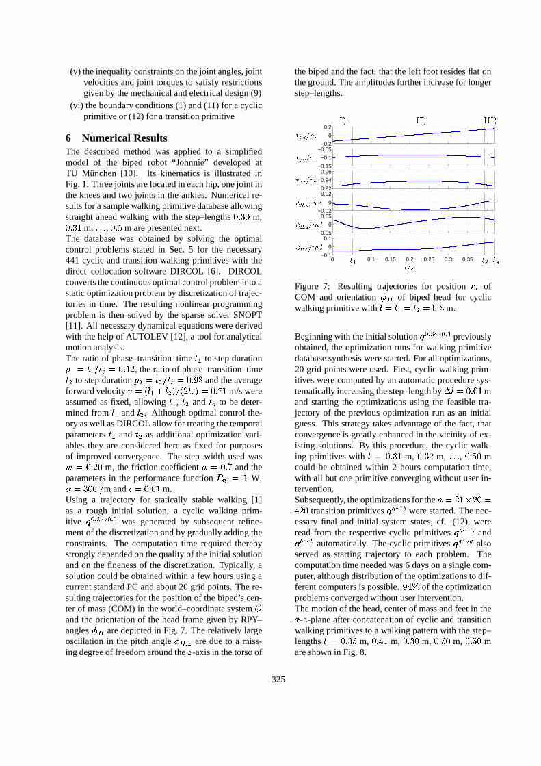
0:3;0:3 was generated by subsequent refine-ment of the discretization and by gradually adding theconstraints. The computation time required therebystrongly depended on the quality of the initial solutionand on the fineness of the discretization. Typically, asolution could be obtained within a few hours using acurrent standard PC and about 20 grid points. The re-sulting trajectories for the position of the biped’s cen-ter of mass (COM) in the world–coordinate systemOand the orientation of the head frame given by RPY–angles�H are depicted in Fig. 7. The relatively largeoscillation in the pitch angle�H;z are due to a miss-ing degree of freedom around thez-axis in the torso of

the biped and the fact, that the left foot resides flat onthe ground. The amplitudes further increase for longerstep–lengths.

−0.2

0

0.2

−0.15

−0.1

−0.05

0.92

0.94

0.96

−0.02

0

0.02

−0.05

0

0.05

0 0.1 0.15 0.2 0.25 0.3 0.35−0.1

0

0.1

rc;y=m

t1 t2t=s

�H;x=rad

�H;y=rad

�H;z=rad

rc;z=m

rc;x=m

I) II) III)

ts

Figure 7: Resulting trajectories for positionrc ofCOM and orientation�H of biped head for cyclicwalking primitive withl = l1 = l2 = 0:3 m:

Beginning with the initial solutionq0:3;0:3 previouslyobtained, the optimization runs for walking primitivedatabase synthesis were started. For all optimizations,20 grid points were used. First, cyclic walking prim-itives were computed by an automatic procedure sys-tematically increasing the step–length by�l = 0:01mand starting the optimizations using the feasible tra-jectory of the previous optimization run as an initialguess. This strategy takes advantage of the fact, thatconvergence is greatly enhanced in the vicinity of ex-isting solutions. By this procedure, the cyclic walk-ing primitives with l = 0:31 m, 0:32 m, : : :, 0:50 mcould be obtained within 2 hours computation time,with all but one primitive converging without user in-tervention.Subsequently, the optimizations for then = 21�20 =

420 transition primitivesqa;b were started. The nec-essary final and initial system states, cf. (12), wereread from the respective cyclic primitivesqa;a andqb;b automatically. The cyclic primitivesqa;a also

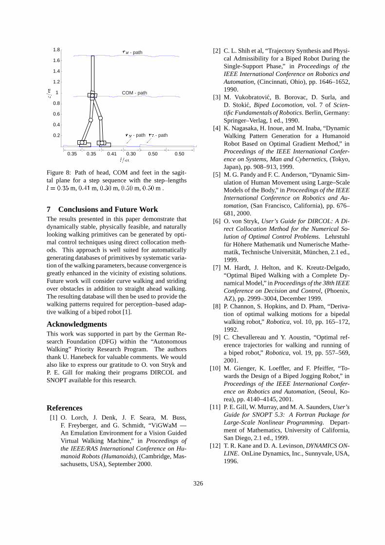
served as starting trajectory to each problem. Thecomputation time needed was 6 days on a single com-puter, although distribution of the optimizations to dif-ferent computers is possible.94% of the optimizationproblems converged without user intervention.The motion of the head, center of mass and feet in thex-z-plane after concatenation of cyclic and transitionwalking primitives to a walking pattern with the step–lengthsl = 0:35 m, 0:41 m, 0:30 m, 0:50 m, 0:50 mare shown in Fig. 8.

325

0.2

0.4

0.6

0.8

1

1.2

1.4

1.6

1.8

COM - path

- path

- path

- path

0.35 0.35 0.41 0.30 0.50 0.50

Figure 8: Path of head, COM and feet in the sagit-tal plane for a step sequence with the step–lengthsl = 0:35 m, 0:41 m, 0:30 m, 0:50 m, 0:50 m .

7 Conclusions and Future WorkThe results presented in this paper demonstrate thatdynamically stable, physically feasible, and naturallylooking walking primitives can be generated by opti-mal control techniques using direct collocation meth-ods. This approach is well suited for automaticallygenerating databases of primitives by systematic varia-tion of the walking parameters, because convergence isgreatly enhanced in the vicinity of existing solutions.Future work will consider curve walking and stridingover obstacles in addition to straight ahead walking.The resulting database will then be used to provide thewalking patterns required for perception–based adap-tive walking of a biped robot [1].

AcknowledgmentsThis work was supported in part by the German Re-search Foundation (DFG) within the “AutonomousWalking” Priority Research Program. The authorsthank U. Hanebeck for valuable comments. We wouldalso like to express our gratitude to O. von Stryk andP. E. Gill for making their programs DIRCOL andSNOPT available for this research.

References[1] O. Lorch, J. Denk, J. F. Seara, M. Buss,

F. Freyberger, and G. Schmidt, “ViGWaM —An Emulation Environment for a Vision GuidedVirtual Walking Machine,” in Proceedings ofthe IEEE/RAS International Conference on Hu-manoid Robots (Humanoids), (Cambridge, Mas-sachusetts, USA), September 2000.

[2] C. L. Shih et al, “Trajectory Synthesis and Physi-cal Admissibility for a Biped Robot During theSingle-Support Phase,” inProceedings of theIEEE International Conference on Robotics andAutomation, (Cincinnati, Ohio), pp. 1646–1652,1990.

[3] M. Vukobratovic, B. Borovac, D. Surla, andD. Stokic, Biped Locomotion, vol. 7 of Scien-tific Fundamentals of Robotics. Berlin, Germany:Springer–Verlag, 1 ed., 1990.

[4] K. Nagasaka, H. Inoue, and M. Inaba, “DynamicWalking Pattern Generation for a HumanoidRobot Based on Optimal Gradient Method,” inProceedings of the IEEE International Confer-ence on Systems, Man and Cybernetics, (Tokyo,Japan), pp. 908–913, 1999.

[5] M. G. Pandy and F. C. Anderson, “Dynamic Sim-ulation of Human Movement using Large–ScaleModels of the Body,” inProceedings of the IEEEInternational Conference on Robotics and Au-tomation, (San Francisco, California), pp. 676–681, 2000.

[6] O. von Stryk,User’s Guide for DIRCOL: A Di-rect Collocation Method for the Numerical So-lution of Optimal Control Problems. Lehrstuhlfur Hohere Mathematik und Numerische Mathe-matik, Technische Universit¨at, Munchen, 2.1 ed.,1999.

[7] M. Hardt, J. Helton, and K. Kreutz-Delgado,“Optimal Biped Walking with a Complete Dy-namical Model,” inProceedings of the 38th IEEEConference on Decision and Control, (Phoenix,AZ), pp. 2999–3004, December 1999.

[8] P. Channon, S. Hopkins, and D. Pham, “Deriva-tion of optimal walking motions for a bipedalwalking robot,”Robotica, vol. 10, pp. 165–172,1992.

[9] C. Chevallereau and Y. Aoustin, “Optimal ref-erence trajectories for walking and running ofa biped robot,”Robotica, vol. 19, pp. 557–569,2001.

[10] M. Gienger, K. Loeffler, and F. Pfeiffer, “To-wards the Design of a Biped Jogging Robot,” inProceedings of the IEEE International Confer-ence on Robotics and Automation, (Seoul, Ko-rea), pp. 4140–4145, 2001.

[11] P. E. Gill, W. Murray, and M. A. Saunders,User’sGuide for SNOPT 5.3: A Fortran Package forLarge-Scale Nonlinear Programming. Depart-ment of Mathematics, University of California,San Diego, 2.1 ed., 1999.

[12] T. R. Kane and D. A. Levinson,DYNAMICS ON-LINE. OnLine Dynamics, Inc., Sunnyvale, USA,1996.

326