Biological Conservation 155 (2012) 1–12

Contents lists available at SciVerse ScienceDirect

Biological Conservation

journal homepage: www.elsevier .com/ locate /biocon

Synergies and trade-offs between ecosystem service supply, biodiversity,and habitat conservation status in Europe

J. Maes a,⇑, M.L. Paracchini a, G. Zulian a, M.B. Dunbar a, R. Alkemade b,c

a Joint Research Centre, Institute for Environment and Sustainability, Via E. Fermi 2749, 21027 Ispra (VA), Italyb PBL Netherlands Environmental Assessment Agency, P.O. Box 303, 3720 AH Bilthoven, The Netherlandsc Environmental Systems Analysis Group, Wageningen University, P.O. Box 47, 6700AA Wageningen, The Netherlands

a r t i c l e i n f o

Article history:Received 28 October 2011Received in revised form 5 June 2012Accepted 11 June 2012Available online 15 July 2012

Keywords:Ecosystem servicesHabitats DirectiveEuropean UnionConservation statusSpatial analysisBiodiversity indicators

0006-3207/$ - see front matter � 2012 Elsevier Ltd. Ahttp://dx.doi.org/10.1016/j.biocon.2012.06.016

⇑ Corresponding author. Address: European CommInstitute for Environment and Sustainability (IES),Resources Unit, Via E. Fermi 2749, 21027 Ispra (VA),fax: +39 0332785819.

E-mail address: joachim.maes@jrc.ec.europa.eu (J.

a b s t r a c t

In the European Union (EU) efforts to conserve biodiversity have been consistently directed towards theprotection of habitats and species through the designation of protected areas under the Habitats Directive(92/43/ECC). These biodiversity conservation efforts also have the potential to maintain or improve thesupply of ecosystem services; however, this potential has been poorly explored across Europe. This paperreports on a spatial assessment of the relationships between biodiversity, ecosystem services, and con-servation status of protected habitats at European scale. We mapped at 10 km resolution ten spatial prox-ies for ecosystem service supply (four provisioning services, five regulating services and one culturalservice) and three proxies for biodiversity (Mean Species Abundance, tree species diversity and the rel-ative area of Natura 2000 sites). Indicators for biodiversity and aggregated ecosystem service supply werepositively related but this relationship was influenced by the spatial trade-offs among ecosystem ser-vices, in particular between crop production and regulating ecosystem services. Using multinomial logis-tic regression models we demonstrated that habitats in a favourable conservation status provided morebiodiversity and had a higher potential to supply, in particular, regulating and cultural ecosystem servicesthan habitats in an unfavourable conservation status. This information is of utmost importance in iden-tifying regions in which measures are likely to result in cost-effective progress towards both new biodi-versity conservation and ecosystem services targets adopted by the Convention on Biological Diversity(CBD) and the EU Biodiversity Strategy to 2020.

� 2012 Elsevier Ltd. All rights reserved.

1. Introduction

The European Union’s Natura 2000 network, established underthe Habitats Directive (92/43/ECC), represents the largest networkof protected sites in the world. At present, the network covers 117million hectares, corresponding to 17% of the surface area of thecountries that constitute the EU. The 1992 Habitats Directive isbased on a conservation approach to biodiversity. In order toachieve its goal of maintaining at, or restoring to, favourable con-servation status, natural and semi-natural habitat types and threa-tened species of wild fauna and flora, a network of protected areaswas established. The Habitats Directive expanded considerably thescope of the 1979 Birds Directive (79/409/EEC) which aims to pro-tect all wild bird species naturally occurring in the EU. Both direc-tives form the legal basis for the European Commission to take the

ll rights reserved.

ission, Joint Research Centre,Rural Water and EcosystemItaly. Tel.: +39 0332789148;

Maes).

necessary measures to protect biodiversity and ecosystems in theEU.

Despite the efforts taken to conserve habitats and species acrossthe EU there is, however, compelling evidence that the ‘‘2010 tar-get’’ of halting or significantly reducing the loss of biodiversity inthe EU as well as at global scale has not been met (Butchartet al., 2010; Hoffmann et al., 2010; Secretariat of the Conventionon Biological Diversity, 2010). The Millennium Ecosystem Assess-ment (MA, 2005) and, more recently, The Economics of Ecosystemsand Biodiversity study (TEEB, 2010) have both increased aware-ness of the negative impacts of biodiversity loss on human welfareby addressing the value of ecosystems and biodiversity for sustain-ing livelihoods, economies, and human wellbeing. Failing to incor-porate the values of ecosystem services and biodiversity intoeconomic decision-making has resulted in investments and activi-ties that degrade natural capital (TEEB, 2010).

In 2010, the tenth meeting of the Conference of Parties (COP 10)to the Convention on Biological Diversity (CBD) led to the adoptionof a global Strategic Plan for biodiversity for the period 2011–2020.The ‘‘2020 Aichi targets’’ complement the previous conservation-based biodiversity targets with the addition of ecosystem services.

2 J. Maes et al. / Biological Conservation 155 (2012) 1–12

Protecting ecosystems and the services they provide to people isassumed to result in positive effects on the conservation of habitatsand species. A similar policy is followed by the EU. The new Biodi-versity Strategy aims to halt the loss of biodiversity and the degra-dation of ecosystem services in the EU by 2020 (EuropeanCommission, 2011). The Strategy contains six targets: first and fore-most to continue conserving nature through completion of theNatura 2000 network and simultaneously ensuring good manage-ment practises in the included protected areas. The second targetuses the argument of ecosystem services to maintain and restoreecosystems through the deployment of a green infrastructure.

The concept of ecosystem services is said to have great potentialin adding value to current conservation approaches, in particularfor local and regional planning (Chan et al., 2006; Daily and Mat-son, 2008; Nelson et al., 2009; Egoh et al., 2009); however, this po-tential remains poorly explored across Europe (Haslett et al., 2010;Harrison et al., 2010).

In this paper we report on a spatial assessment of the relation-ships between biodiversity, ecosystem services, and conservationstatus of protected habitats at European scale. The hypothesis isthat habitats in a favourable conservation status provide higherlevels across multiple ecosystem services and host a richer biodi-versity than habitats in unfavourable conservation status. Usingspatial datasets of habitat conservation status, ecosystem servicesupply, and biodiversity covering the EU, we present evidence thatsupports this hypothesis. Our approach consisted of three parts:Firstly, we mapped spatially explicit indicators for biodiversityand ecosystem services at EU scale. Then we analysed the spatialconcordance between multiple ecosystem services and biodiver-sity. Finally we analysed the relationship between habitat conser-vation status, ecosystem services, and biodiversity.

2. Methods

2.1. Spatial indicators for land cover, ecosystem services andbiodiversity

We mapped the European distribution of different proxies forland cover, ecosystem service supply and biodiversity at a 10 kmresolution using a reference grid system (EEA, 2007). Here we pro-

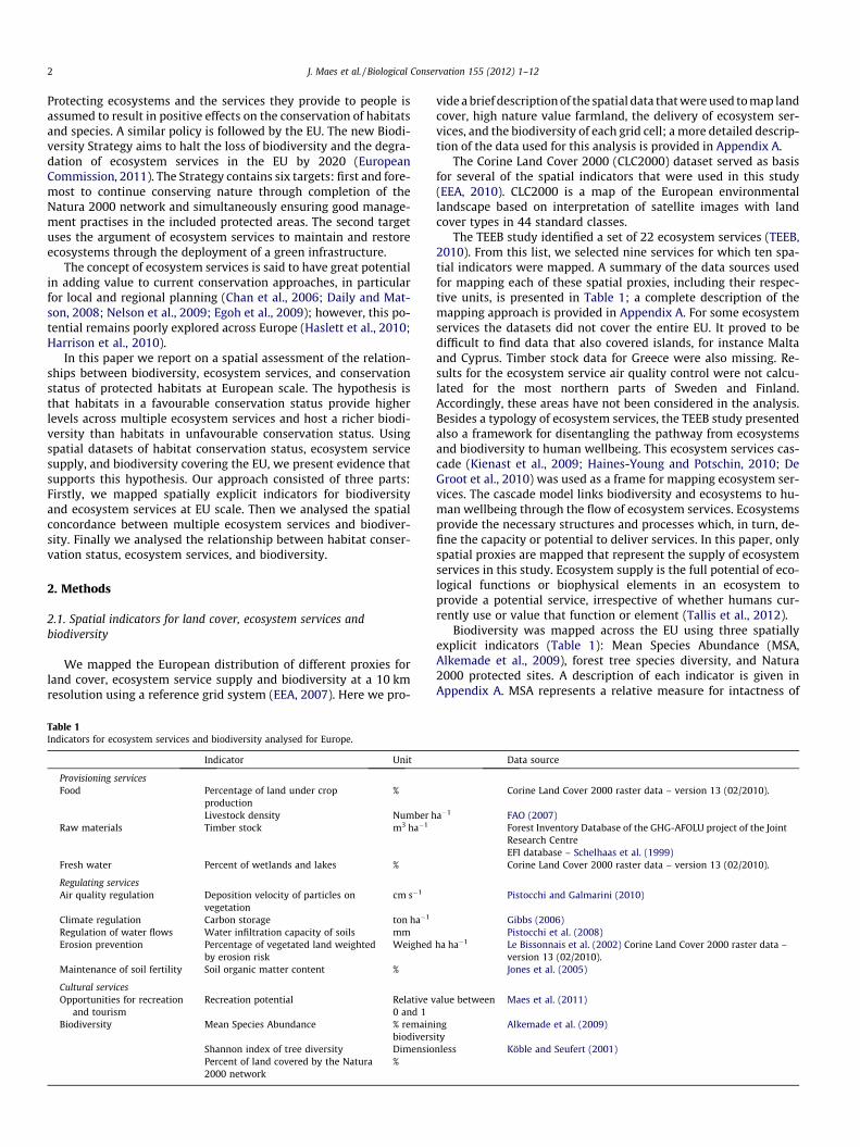
Table 1Indicators for ecosystem services and biodiversity analysed for Europe.

Indicator Unit

Provisioning servicesFood Percentage of land under crop

production%

Livestock density Number hRaw materials Timber stock m3 ha�1

Fresh water Percent of wetlands and lakes %

Regulating servicesAir quality regulation Deposition velocity of particles on

vegetationcm s�1

Climate regulation Carbon storage ton ha�1

Regulation of water flows Water infiltration capacity of soils mmErosion prevention Percentage of vegetated land weighted

by erosion riskWeighed

Maintenance of soil fertility Soil organic matter content %

Cultural servicesOpportunities for recreation

and tourismRecreation potential Relative v

0 and 1Biodiversity Mean Species Abundance % remain

biodiversShannon index of tree diversity DimensioPercent of land covered by the Natura2000 network

%

vide a brief description of the spatial data that were used to map landcover, high nature value farmland, the delivery of ecosystem ser-vices, and the biodiversity of each grid cell; a more detailed descrip-tion of the data used for this analysis is provided in Appendix A.

The Corine Land Cover 2000 (CLC2000) dataset served as basisfor several of the spatial indicators that were used in this study(EEA, 2010). CLC2000 is a map of the European environmentallandscape based on interpretation of satellite images with landcover types in 44 standard classes.

The TEEB study identified a set of 22 ecosystem services (TEEB,2010). From this list, we selected nine services for which ten spa-tial indicators were mapped. A summary of the data sources usedfor mapping each of these spatial proxies, including their respec-tive units, is presented in Table 1; a complete description of themapping approach is provided in Appendix A. For some ecosystemservices the datasets did not cover the entire EU. It proved to bedifficult to find data that also covered islands, for instance Maltaand Cyprus. Timber stock data for Greece were also missing. Re-sults for the ecosystem service air quality control were not calcu-lated for the most northern parts of Sweden and Finland.Accordingly, these areas have not been considered in the analysis.Besides a typology of ecosystem services, the TEEB study presentedalso a framework for disentangling the pathway from ecosystemsand biodiversity to human wellbeing. This ecosystem services cas-cade (Kienast et al., 2009; Haines-Young and Potschin, 2010; DeGroot et al., 2010) was used as a frame for mapping ecosystem ser-vices. The cascade model links biodiversity and ecosystems to hu-man wellbeing through the flow of ecosystem services. Ecosystemsprovide the necessary structures and processes which, in turn, de-fine the capacity or potential to deliver services. In this paper, onlyspatial proxies are mapped that represent the supply of ecosystemservices in this study. Ecosystem supply is the full potential of eco-logical functions or biophysical elements in an ecosystem toprovide a potential service, irrespective of whether humans cur-rently use or value that function or element (Tallis et al., 2012).

Biodiversity was mapped across the EU using three spatiallyexplicit indicators (Table 1): Mean Species Abundance (MSA,Alkemade et al., 2009), forest tree species diversity, and Natura2000 protected sites. A description of each indicator is given inAppendix A. MSA represents a relative measure for intactness of

Data source

Corine Land Cover 2000 raster data – version 13 (02/2010).

a�1 FAO (2007)Forest Inventory Database of the GHG-AFOLU project of the JointResearch CentreEFI database – Schelhaas et al. (1999)Corine Land Cover 2000 raster data – version 13 (02/2010).

Pistocchi and Galmarini (2010)

Gibbs (2006)Pistocchi et al. (2008)

ha ha�1 Le Bissonnais et al. (2002) Corine Land Cover 2000 raster data –version 13 (02/2010).Jones et al. (2005)

alue between Maes et al. (2011)

ingity

Alkemade et al. (2009)

nless Köble and Seufert (2001)

J. Maes et al. / Biological Conservation 155 (2012) 1–12 3

ecosystems calculated using the GLOBIO3 model (Verboom et al.,2007; Alkemade et al., 2009) and is similar to the BiodiversityIntactness Index (Scholes and Biggs, 2005).

2.2. Assessment of habitat conservation status

Spatial data on the conservation status of habitats were takenfrom an EU wide habitat assessment. The legal basis for this assess-ment is Article 17 of the EU Habitats Directive which requires thatEU Member States evaluate every six years the conservation statusof habitats and species that are listed in the annexes of the direc-tive. Habitat status was not assessed at local scale but across an en-tire bio-geographical region within each Member State. Theassessment assigned favourable (FV), unfavourable-inadequate(U1) or unfavourable-bad (U2) conservation status to 216 differenthabitats across 25 Member States covering seven terrestrial andfour marine bio-geographical regions (totalling 2759 habitatassessments). We restricted our analysis to the seven terrestrialbiogeographical regions so we did not consider marine habitatsin this analysis. All national assessments were collected by theEuropean Topic Centre on Biological Diversity (ETC/BD) and areavailable in a geospatial database reporting habitat conservationstatus on a 10 km grid covering the EU-25. More information isavailable in Appendix A. From the dataset including 2759 habitatassessments, we removed all the assessments of marine habitatsand all the assessments that resulted in an unknown conservationstatus. This final dataset included 1889 habitat assessments. Eachassessment was then spatially joined as an attribute to a GISshapefile with polygons that describe the presence of each habitaton the 10 km resolution grid.

2.3. Statistical analysis

2.3.1. Multiple ecosystem servicesWe used a correlation biplot based on principal component

analysis (PCA) to detect spatial synergies and trade-offs among ser-vices. We used the first three principal components as proxies formultiple services for further correlation analysis. Prior to PCAand following Lavorel et al. (2011), we standardized the differentecosystem service maps between 0 and 1 based on minimumand maximum values. These maps were summed to create mapsof multiple ecosystem services depending on the correlation struc-ture that was revealed by the PCA. In addition, all standardizedecosystem service maps were summed to a single aggregate indi-cator, Total Ecosystem Service Value (TESV), representing thecapacity of each grid cell to provide multiple services. TESV thusassumed that each ecosystem service is valued the same.

Relationships between the first three principal components andland cover were analysed using Pearson correlation coefficients.Hereto, we calculated the proportion of land cover types in each10 km grid cell using the label 2 classification of the CLC2000 data-set. A similar analysis correlated the principal components withthe three biodiversity indicators. Finally, we related the principalcomponents to the spatial distribution of high nature value farm-land in Europe (HNV). HNV farmlands are areas in Europe whereagriculture supports, or is associated with, a high species and hab-itat diversity (Paracchini et al., 2008; Doxa et al., 2010). The sup-plementary information in Appendix A provides details on theHNV map that was used to calculate the average percentage ofHNV farmland in each 10 km grid cell.

2.3.2. Correlation between biodiversity and ecosystem servicesWe calculated spatial correlations between TESV, MSA, forest

tree species diversity and the relative surface area of protectedsites using the Modified t-test for correlation. This procedure calcu-

lates Pearson’s product–moment correlation between two vari-ables and tests its significance following the procedure describedin Clifford et al. (1989) (CRH-test). The CRH-test corrects the de-grees of freedom, based on the amount of autocorrelation in thedata, using Moran’s I to estimate the spatial autocorrelation inthe data sets. The corrected degrees of freedom are then used totest the significance of the correlation. The test was based on a ran-dom selection of 1000 grid cells.

2.3.3. Multinomial logistic regressionMultinomial logistic regression is used to predict the probabil-

ity of category membership on a dependent variable based on anindependent variable. The procedure is a simple extension of bin-ary logistic regression that allows for more than two categoriesof the dependent or outcome variable. Here, we modelled the prob-ability of habitat conservation status as a function of ecosystemservices or biodiversity using univariate multinomial logisticregression models with a generalized logit link. The dependent var-iable had three possible discrete outcomes: favourable conserva-tion status (FV), unfavourable–inadequate conservation status(U1) or unfavourable–bad conservation status (U2).

We intersected each of the 1889 habitat conservation statusmaps with the ecosystem services and biodiversity maps in orderto extract a data set with the assessment class as categoricaldependent variable (FV, U1 or U2) and biodiversity or ecosystemservice indicators as continuous independent variable.

In a multinomial logistic regression model, the estimates for theparameters can be identified compared to a baseline category. Inour study the probability of membership in the categories FV andU1 was compared to the probability of membership in a referencecategory (U2). The multinomial logistic regression model with ref-erence category U2 can be expressed as follows:

logpi

pU2

� �¼ b1i þ b2ix

where pi is the probability of class membership in the categories FVor U1, pU2 is the probability of class membership in the referencecategory U2; x is the independent or predictor variable and b1i

and b2i are the regression coefficients that were estimated usingmaximum likelihood. Model goodness-of-fit was evaluated usingthe chi squared statistic.

2.3.4. Uncertainty analysisThe Article 17 reporting on habitat and species conservation

status constituted an unparalleled assessment involving hundredsof people in national and regional administrations and researchinstitutes from 25 EU Member States (European Commission,2009). However, it was not realistic to assess European habitatsusing a harmonized approach throughout all Member States. Thisresulted in two main problems: (i) the use of a different baselineto assess conservation status of habitats and (ii) differences in spa-tial accuracy of the data. The European Topic Centre on BiologicalDiversity provided a detailed report on the completeness, qualityand coherence of the data (ETC/BD, 2008).

We used a Monte Carlo analysis to test the robustness of theregression coefficients obtained from the multinomial logitmodels. We randomly resampled 200 habitat assessments out ofa total of 1889 habitat assessments and recalculated the regressioncoefficients b1i and b2i. We repeated this procedure 500 times. Thisresulted in a distribution representing the uncertainty in eachof the four model parameters, which is explained by a normaldistribution.

4 J. Maes et al. / Biological Conservation 155 (2012) 1–12

3. Results

3.1. Spatial patterns in biodiversity and ecosystem service supply

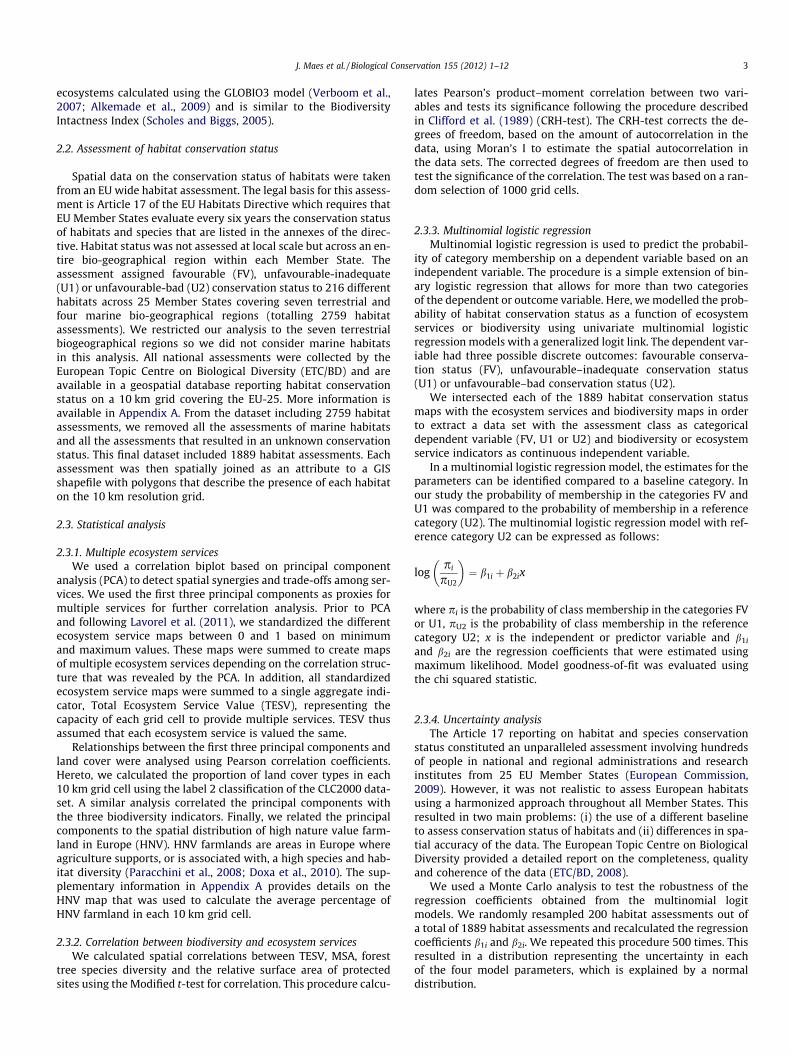
In Europe, the supply of multiple ecosystem services (TESV) waslow in the densely populated areas of the Atlantic plane and north-ern Italy as well as in areas with intensive agriculture and livestockproduction in Spain, Ireland and the United Kingdom (Fig. 1). TESVwas high in areas with dense forest cover, in particular mountains,and regions rich in wetlands such as north-west Ireland or Swedenand Finland.

Fig. 1. Biodiversity and ecosystem services maps (European Union, 10 km resolution gridvalues for of 10 ecosystem service indicators. Data for timber stock for Greece were missnot included. Results for air quality control were not calculated for the northern areas of Sof protected areas which are part of the Natura 2000 network. Bottom right: The forestcalculated from a 1 km resolution grid.

The proxies used for biodiversity also revealed an uneven distri-bution across Europe (Fig. 1). Tree species diversity resulted in highvalues in Scandinavia as well as for major mountain chains that arepresent on the continent. A spatial map of MSA, a modelled biodi-versity indicator, showed that the remaining European biodiversitywas situated in the northern parts of the continent as well as in theless exploited mountain areas, for instance Slovenia, and larger is-lands. Furthermore, different country specific approaches to estab-lishing the Natura 2000 network are evident. Some countriescreated a dense network of relatively small sites (e.g. Germany)while others focussed on larger areas and national parks (e.g.France, Italy) or on river networks (e.g. Poland).

cells). Top left: Total ecosystem service supply calculated as the sum of standardizeding. Also for several islands not all the services could be calculated and are thereforeweden and Finland. Top right: Mean Species Abundance. Bottom left: The proportiontree species diversity measured using the average Shannon Wiener Diversity Index

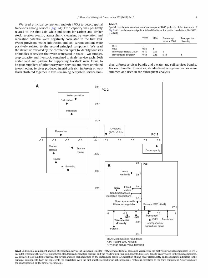
Table 2Spatial correlations based on a random sample of 1000 grid cells of the four maps ofFig. 1. All correlations are significant (Modified t-test for spatial correlations, N = 1000,p < 0.05).

TESV MSA PercentageNatura 2000

Tree speciesdiversity

TESV 1MSA 0.51 1Percentage Natura 2000 0.40 0.13 1Tree species diversity 0.43 0.45 0.11 1

J. Maes et al. / Biological Conservation 155 (2012) 1–12 5

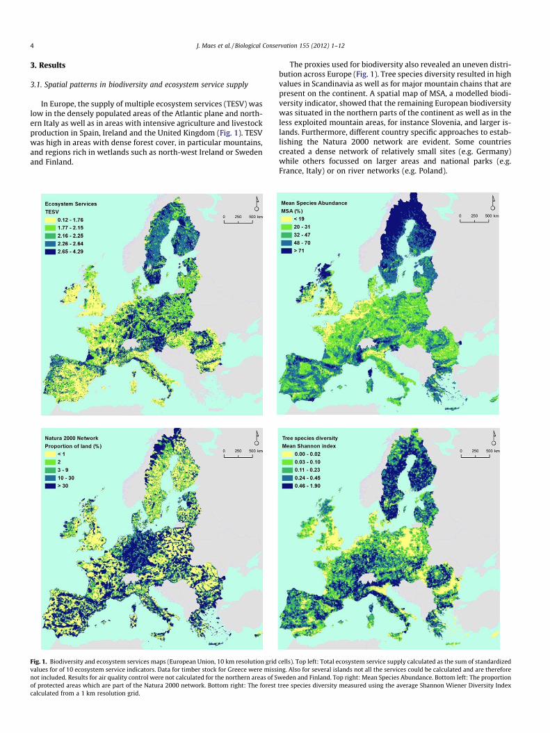
We used principal component analysis (PCA) to detect spatialtrade-offs among services (Fig. 2A). Crop capacity was positivelyrelated to the first axis while indicators for carbon and timberstock, erosion control, atmospheric cleansing by vegetation andrecreation potential were negatively correlated to the first axis.Water provision, water infiltration and soil carbon content werepositively related to the second principal component. We usedthe structure revealed by the correlation biplot to identify four setsor bundles of services that were segregated in space: Two bundles,crop capacity and livestock, contained a single service each. Botharable land and pasture for supporting livestock were found tobe poor suppliers of other ecosystem services and were unrelatedto each other. Services produced in grid cells rich in forests or wet-lands clustered together in two remaining ecosystem service bun-

Water provision

Carbonstorage

Air cleansing

Erosion control

Infiltration

Timber

Recreation

Soil carbon

-0.9

-0.6

-0.3

0.0

0.3

0.6

0.9

-0.9 -0.7 -0.5 -0.3 -0.1 0.1

PC 2

-1

ve

A

B

MNH

Fig. 2. A. Principal component analysis of ecosystem services at European scale (N = 404Each dot represents the correlation between standardized ecosystem services and the twWe extracted four bundles of services for further analysis each identified by the rectanguprincipal components. Each dot represents the correlation with the first and the secondthe exact position on the first or second axis.

dles: a forest services bundle and a water and soil services bundle.For each bundle of services, standardized ecosystem values weresummed and used in the subsequent analysis.

Crop capacity

Livestock (PC3: -0.81)

0.3 0.5 0.7 0.9

PC 1

-0.4

-0.2

0

0.2

0.4

0.6

0.8

-0.5 0 0.5 1N2K

Arable landHeterogeneous

agricultural areas

Permanentcrops

Pasture (PC3: -0.41)

Forests

Open spaces with little or no vegetation

Scrub/herbaceous getation associations

Inlandwaters

Inlandwetlands

PC 1

PC 2

HNV

MSA

Tree speciesdiversity

SA: Mean Species Abundance2K: Natura 2000 networkNV: High Nature Value farmland

26 grid cells; total explained variance by the first two principal components is 47%).o first principal components. Livestock density is correlated to the third component.lar boxes. B. Correlation of land cover classes, HNV and biodiversity indicators to theprincipal component. Pasture is correlated to the third component. Arrows indicate

0.00 0.25 0.50 0.75 1.00 1.25 1.50 1.75 2.00

-0.1

0

0.1

0.2

0.3

0.4

0.5

0.6

0.7

0.8

0.9

0 20 40 60 80 100

Tree species diversity

Cro

plan

d

Mean Species Abundance (%)Natura 2000 area (%)

0.00 0.25 0.50 0.75 1.00 1.25 1.50 1.75 2.00

0

0.1

0.2

0.3

0.4

0.5

0.6

0.7

0.8

0.9

1

0 20 40 60 80 100

Tree species diversity

Wat

er a

nd s

oil s

ervi

ces

Mean Species Abundance (%)Natura 2000 area (%)

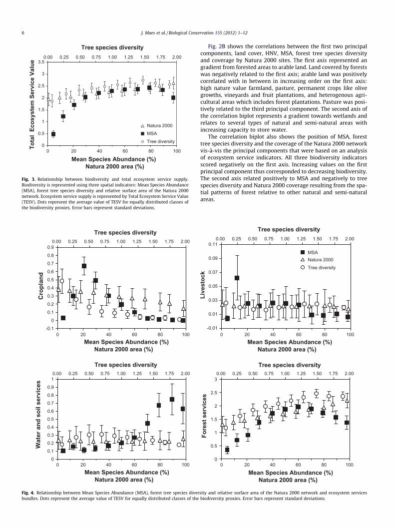
Fig. 4. Relationship between Mean Species Abundance (MSA), forest tree species diverbundles. Dots represent the average value of TESV for equally distributed classes of the

0.00 0.25 0.50 0.75 1.00 1.25 1.50 1.75 2.00

0

0.5

1

1.5

2

2.5

3

3.5

0 20 40 60 80 100

Tree species diversity

Tota

l Ec

osys

tem

Ser

vice

Val

ue

Mean Species Abundance (%)Natura 2000 area (%)

Natura 2000

MSA

Tree diversity

Fig. 3. Relationship between biodiversity and total ecosystem service supply.Biodiversity is represented using three spatial indicators: Mean Species Abundance(MSA), forest tree species diversity and relative surface area of the Natura 2000network. Ecosystem service supply is represented by Total Ecosystem Service Value(TESV). Dots represent the average value of TESV for equally distributed classes ofthe biodiversity proxies. Error bars represent standard deviations.

6 J. Maes et al. / Biological Conservation 155 (2012) 1–12

Fig. 2B shows the correlations between the first two principalcomponents, land cover, HNV, MSA, forest tree species diversityand coverage by Natura 2000 sites. The first axis represented angradient from forested areas to arable land. Land covered by forestswas negatively related to the first axis; arable land was positivelycorrelated with in between in increasing order on the first axis:high nature value farmland, pasture, permanent crops like olivegrowths, vineyards and fruit plantations, and heterogenous agri-cultural areas which includes forest plantations. Pasture was posi-tively related to the third principal component. The second axis ofthe correlation biplot represents a gradient towards wetlands andrelates to several types of natural and semi-natural areas withincreasing capacity to store water.

The correlation biplot also shows the position of MSA, foresttree species diversity and the coverage of the Natura 2000 networkvis-à-vis the principal components that were based on an analysisof ecosystem service indicators. All three biodiversity indicatorsscored negatively on the first axis. Increasing values on the firstprincipal component thus corresponded to decreasing biodiversity.The second axis related positively to MSA and negatively to treespecies diversity and Natura 2000 coverage resulting from the spa-tial patterns of forest relative to other natural and semi-naturalareas.

0.00 0.25 0.50 0.75 1.00 1.25 1.50 1.75 2.00

-0.01

0.01

0.03

0.05

0.07

0.09

0.11

0 20 40 60 80 100

Tree species diversity

Live

stoc

k

Mean Species Abundance (%)Natura 2000 area (%)

MSANatura 2000Tree diversity

0.00 0.25 0.50 0.75 1.00 1.25 1.50 1.75 2.00

0

0.5

1

1.5

2

2.5

3

0 20 40 60 80 100

Tree species diversity

Fore

st s

ervi

ces

Mean Species Abundance (%)Natura 2000 area (%)

sity and relative surface area of the Natura 2000 network and ecosystem servicesbiodiversity proxies. Error bars represent standard deviations.

J. Maes et al. / Biological Conservation 155 (2012) 1–12 7

3.2. Spatial concordance between ecosystem services and biodiversity

Significantly positive correlations (Modified t-test for spatialcorrelations, N = 1000, p < 0.05) were reported among the threebiodiversity indicators (Table 2). MSA related best with tree speciesdiversity. Spatial mismatches between these two proxies are evi-dent from the maps (Fig. 2) since the forest tree species data arebased on field plots, whereas MSA mainly reflects land use inten-sity. In regions where forest plantations have replaced natural veg-etation, such as the Landes in south-west France, MSAoverestimated biodiversity. Although significant, the relationshipbetween relative surface area of protected sites and both MSAand forest tree species diversity was weak (Table 2), thus suggest-ing that much of Europe’s remaining biodiversity is still found out-side protected areas.

We found significantly positive correlations between ecosystemservices and the spatial proxies for biodiversity (Table 2, Modifiedt-test for spatial correlations, N = 1000, p < 0.05). We found a satu-rating relationship between TESV and MSA (Fig. 3). Increasing MSAfrom values below 60% resulted in clear increments of TESV but therelationship reached a maximum at values above 60%. The trade-offs that exist among ecosystem services yielded different relation-ships with MSA (Fig. 4). High MSA was associated with low provi-

0

0.1

0.2

0.3

0.4

0.5

0.6

0.7

0 20 40 60 80 100

Prob

abili

ty o

f con

serv

atio

n st

atus

Mean Species Abundance (%)

0

0.1

0.2

0.3

0.4

0.5

0.6

0.7

0.8

0.9

1

0 0.25 0.5 0.75 1 1.25 1.5 1.75 2

Prob

abili

ty o

f con

serv

atio

n st

atus

Forest tree species divesity

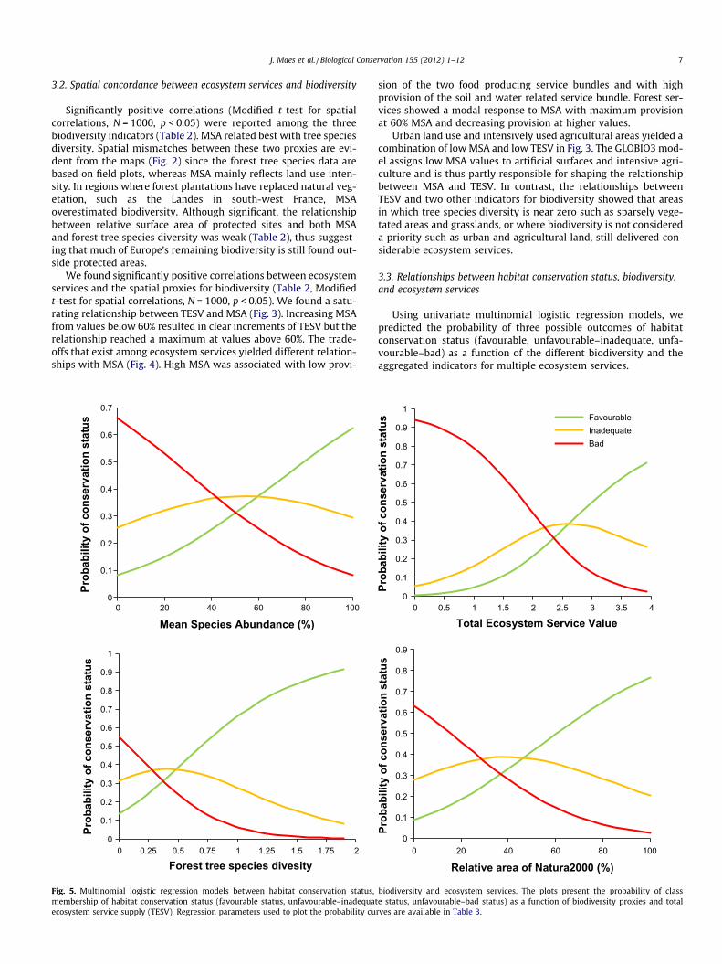
Fig. 5. Multinomial logistic regression models between habitat conservation status,membership of habitat conservation status (favourable status, unfavourable–inadequatecosystem service supply (TESV). Regression parameters used to plot the probability cu

sion of the two food producing service bundles and with highprovision of the soil and water related service bundle. Forest ser-vices showed a modal response to MSA with maximum provisionat 60% MSA and decreasing provision at higher values.

Urban land use and intensively used agricultural areas yielded acombination of low MSA and low TESV in Fig. 3. The GLOBIO3 mod-el assigns low MSA values to artificial surfaces and intensive agri-culture and is thus partly responsible for shaping the relationshipbetween MSA and TESV. In contrast, the relationships betweenTESV and two other indicators for biodiversity showed that areasin which tree species diversity is near zero such as sparsely vege-tated areas and grasslands, or where biodiversity is not considereda priority such as urban and agricultural land, still delivered con-siderable ecosystem services.

3.3. Relationships between habitat conservation status, biodiversity,and ecosystem services

Using univariate multinomial logistic regression models, wepredicted the probability of three possible outcomes of habitatconservation status (favourable, unfavourable–inadequate, unfa-vourable–bad) as a function of the different biodiversity and theaggregated indicators for multiple ecosystem services.

0

0.1

0.2

0.3

0.4

0.5

0.6

0.7

0.8

0.9

1

0 0.5 1 1.5 2 2.5 3 3.5 4

Prob

abili

ty o

f con

serv

atio

n st

atus

Total Ecosystem Service Value

FavourableInadequateBad

0

0.1

0.2

0.3

0.4

0.5

0.6

0.7

0.8

0.9

0 20 40 60 80 100

Prob

abili

ty o

f con

serv

atio

n st

atus

Relative area of Natura2000 (%)

biodiversity and ecosystem services. The plots present the probability of classe status, unfavourable–bad status) as a function of biodiversity proxies and totalrves are available in Table 3.

8 J. Maes et al. / Biological Conservation 155 (2012) 1–12

Increasing biodiversity indicator values resulted in an increaseof the probability of a favourable conservation status while theprobability of an unfavourable–bad conservation status decreased(Fig. 5). A modal response was observed for unfavourable–inade-quate conservation status. All models were significant (Multino-mial logit regression; N = 1889; X2

df¼2 > 5:99 at p = 0.05) andyielded significant regression coefficients as well (Table 3).

We found a similar relationship between TESV and habitat con-servation status (Fig. 5). The probability that habitats are in favour-able conservation status increased with increasing values for TESV.The opposite relationship existed between TESV and habitats inunfavourable–bad conservation status. Also here, the regressionmodel produced significant parameters (Table 3).

The response of conservation status differed when different ser-vice bundles were considered (Fig. 6). Unfavourable–bad habitatconservation status was predicted to increase with increasing val-ues of food producing service systems. Favourable habitat conser-vation status is predicted to increase with increasing values of theforest services bundle and the water and soil services bundle. How-ever, for the latter model, the regression coefficients were not sig-nificant at p < 0.05 (Table 3).

3.4. Uncertainty analysis

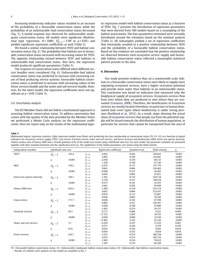
The EU Member States did not follow a harmonized approach toassessing habitat conservation status. To address uncertainty thatcomes with the quality of the data provided by the Member Stateswe performed a Monte Carlo analysis on the regression coeffi-cients. Here we report only on the results of the multinomial logis-

Table 3Multinomial logistic regression statistics. Eight regression models were fitted, each predicindicators for ecosystem services supply (TESV, crop service, livestock service, water andrelative surface area of Natura 2000 sites). Overall goodness of fit of the model was testedtogether with their standard deviation and the significance level (p). The significance of th

Independent variables Likelihood ratio test R

TESVaX2

df ¼ 2 145.4 b1, FV

b2, FV

p <0.001 b1, U1

b2, U1

MSA X2df ¼ 2 139.2 b1, FV

b2, FV

p <0.001 b1, U1

b2, U1

Forest tree species diversity X2df ¼ 2 160.1 b1, FV

b2, FV

p <0.001 b1, U1

b2, U1

Natura 2000 sites X2df ¼ 2 263.2 b1, FV

b2, FV

p <0.001 b1, U1

b2, U1

Crop services X2df ¼ 2 171.7 b1, FV

b2, FV

p <0.001 b1, U1

b2, U1

Livestock services X2df ¼ 2 45.3 b1, FV

b2, FV �p <0.001 b1, U1

b2, U1 �Water and soil services X2

df ¼ 2 3.7 b1, FV

b2, FV

p 0.16 b1, U1

b2, U1

Forest services X2df ¼ 2 223.1 b1, FV

b2, FV

p <0.001 b1, U1

b2, U1

FV = Favourable habitat conservation status; U1: Unfavourable–inadequate habitat consa Results of a Monte Carlo analysis on this model are available in Fig. 7.

tic regression model with habitat conservation status as a functionof TESV. Fig. 7 presents the distribution of regression parametersthat were derived from 500 models based on a resampling of thehabitat assessments. The four parameters estimated were normallydistributed around the estimates based on the nominal analysis(Table 3). All subsamples yielded a set of regression coefficientsthat invariantly resulted in a positive relationship between TESVand the probability of a favourable habitat conservation status.Based on this evidence we concluded that the positive relationshipwe observed between total ecosystem service supply and favour-able habitat conservation status reflected a meaningful statisticalpattern present in the data.

4. Discussion

Our study presents evidence that, on a countrywide scale, hab-itats in a favourable conservation status were likely to supply moreregulating ecosystem services, have a higher recreation potentialand provide more water than habitats in an unfavourable status.This conclusion was based on indicators that measured only thebiophysical supply of ecosystem services. Ecosystem services flowfrom sites where they are produced to sites where they are con-sumed (Costanza, 2008). Therefore, the beneficiaries of ecosystemservices are mostly located elsewhere, in particular in human dom-inated land cover types where biodiversity is under strong pres-sure (Burkhard et al., 2012). As a result, maps showing the actualshare of ecosystem services that people use from the potential sup-ply will be biased towards the distribution of human population, inparticular for services that cannot be transported from the area of

ting the class membership or conservation status (FV, U1, U2) as a function of spatialsoil services, and forest services) and biodiversity (MSA, forest tree species diversity,

using a likelihood ratio test. For each model, the parameter estimates are presentede model parameters was tested using the Wald statistic.

egression coefficient Standard error Wald statistic p

�4.923 0.434 128.922 <0.0012.097 0.190 122.041 <0.001�2.930 0.378 60.133 <0.001

1.330 0.169 61.742 <0.001�2.075 0.177 137.770 <0.001

0.041 0.004 126.462 <0.001�0.948 0.157 36.492 <0.001

0.022 0.003 41.651 <0.001�1.391 0.116 144.118 <0.001

3.736 0.315 140.234 <0.001�0.573 0.101 32.255 <0.001

2.041 0.302 45.694 <0.001�1.969 0.134 216.119 <0.001

0.053 0.004 215.437 <0.001�0.819 0.112 53.867 <0.001

0.028 0.003 70.438 <0.0010.836 0.102 67.700 <0.001�4.065 0.331 150.591 <0.001

0.506 0.100 25.600 <0.001�1.662 0.276 36.157 <0.001

0.177 0.086 4.221 0.04017.372 2.965 34.335 <0.001

0.284 0.080 12.550 <0.00111.863 2.522 22.126 <0.001�0.358 0.107 11.252 0.001

0.571 0.356 2.570 0.1090.016 0.102 0.025 0.874�0.054 0.353 0.024 0.878�3.761 0.274 188.738 <0.001

2.073 0.153 182.733 <0.001�1.963 0.224 76.610 <0.001

1.203 0.133 82.320 <0.001

ervation status; U2: Unfavourable–bad habitat conservation status.

0

0.1

0.2

0.3

0.4

0.5

0.6

0.7

0.8

0 0.2 0.4 0.6 0.8 1

Prob

abili

ty o

f con

serv

atio

n st

atus

Crop capacity

FavourableInadequateBad

0

0.1

0.2

0.3

0.4

0.5

0.6

0.7

0.8

0 0.02 0.04 0.06 0.08 0.1 0.12 0.14

Prob

abili

ty o

f con

serv

atio

n st

atus

Grazing livestock

0

0.1

0.2

0.3

0.4

0.5

0.6

0.7

0.8

0.9

1

0 0.5 1 1.5 2 2.5 3 3.5

Prob

abili

ty o

f con

serv

atio

n st

atus

Forest services

0.25

0.27

0.29

0.31

0.33

0.35

0.37

0.39

0.41

0 0.2 0.4 0.6 0.8 1

Prob

abili

ty o

f con

serv

atio

n st

atus

Water and soil services

Fig. 6. Multinomial logistic regression models between habitat conservation status, biodiversity and ecosystem service bundles. The plots present the probability of classmembership of habitat conservation status (favourable status, unfavourable–inadequate status, unfavourable–bad status) as a function of biodiversity proxies and totalecosystem service supply (TESV). Regression parameters used to plot the probability curves are available in Table 3.

J. Maes et al. / Biological Conservation 155 (2012) 1–12 9

production to the area of consumption. The complexity of tracingthe spatial and temporal quantitative differences between supplyand demand of ecosystem services remains a constraint on thedevelopment of maps of demand and actual use of ecosystem ser-vices. For some services, such as food and timber or climate and airquality regulation, a global approach to mapping ecosystem ser-vices is needed to unravel the flows between regions, countries,and continents, whereas water related services require a river ba-sin based approach. To be consistent in our approach to mappingecosystem service supply, we used exclusively biophysical proxiesthat have been presented in other, leading studies, thus enablingcomparison among maps across scales: crop production capacity(Raudsepp-Hearne et al., 2010), timber stock (Schröter et al.,2005), carbon storage (Chan et al., 2006; Schröter et al., 2005; Egohet al., 2009; Naidoo et al., 2010; Raudsepp-Hearne et al., 2010),water infiltration capacity of soils (Rey Benayas et al., 2009), ero-sion (Egoh et al., 2009), soil organic matter content (Schröteret al., 2005; Raudsepp-Hearne et al., 2010; Rey Benayas et al.,2009), and recreation (Raudsepp-Hearne et al., 2010).

Clearly, land cover and land use explain a considerable part ofthe variation in the spatial supply of ecosystem services in Europe.The data used in this study suggest that crop and livestock produc-tion, both provisioning services, create trade-offs with regulatingecosystem services considered in this study, water provision and

recreation. Land parcels rich in agro-ecosystems essentially pro-duce crops or livestock and are relatively poor in delivering otherecosystem services. Land parcels rich in forests or wetlands pro-vide a wide array of services. They have high potential to store car-bon, aid in erosion and air quality control, provide recreation andtimber, and support the regulation of soils and water. Trade-offsbetween provisioning and regulating ecosystem services at differ-ent scales have been identified as cause for concern, because regu-lating ecosystem services are thought to underpin the sustainableproduction of provisioning and cultural ecosystem services (Rodrí-guez et al., 2006; Raudsepp-Hearne et al., 2010). Regional landmanagement has favoured the production of crops and livestock,and has reduced the capacity of ecosystems to provide water orregulating and cultural services. However, this process is not nec-essarily irreversible. Good management of ecosystems may turntrade-offs that arise at regional scale into opportunities for syner-gies among ecosystem services at local scale. Good agriculturalpractices, such as nutrient buffer strips, green cover during winteror crop diversification may increase the capacity of cropland forinfiltration and consequently decrease water runoff rates. Thiswould in turn increase biodiversity and habitat for pollinators orimprove erosion control. An example is provided by HNV farmland.This type of farmland is defined as low-intensity farmland support-ing or associated with a high biodiversity rate, in terms of species

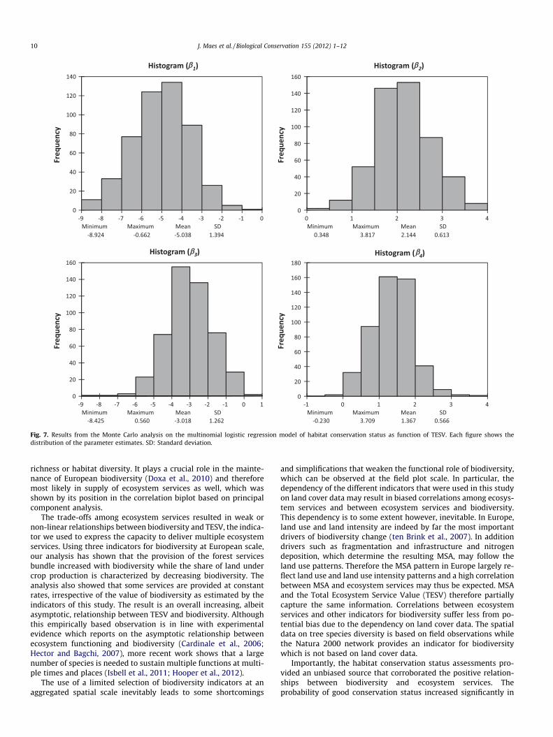
Fig. 7. Results from the Monte Carlo analysis on the multinomial logistic regression model of habitat conservation status as function of TESV. Each figure shows thedistribution of the parameter estimates. SD: Standard deviation.

10 J. Maes et al. / Biological Conservation 155 (2012) 1–12

richness or habitat diversity. It plays a crucial role in the mainte-nance of European biodiversity (Doxa et al., 2010) and thereforemost likely in supply of ecosystem services as well, which wasshown by its position in the correlation biplot based on principalcomponent analysis.

The trade-offs among ecosystem services resulted in weak ornon-linear relationships between biodiversity and TESV, the indica-tor we used to express the capacity to deliver multiple ecosystemservices. Using three indicators for biodiversity at European scale,our analysis has shown that the provision of the forest servicesbundle increased with biodiversity while the share of land undercrop production is characterized by decreasing biodiversity. Theanalysis also showed that some services are provided at constantrates, irrespective of the value of biodiversity as estimated by theindicators of this study. The result is an overall increasing, albeitasymptotic, relationship between TESV and biodiversity. Althoughthis empirically based observation is in line with experimentalevidence which reports on the asymptotic relationship betweenecosystem functioning and biodiversity (Cardinale et al., 2006;Hector and Bagchi, 2007), more recent work shows that a largenumber of species is needed to sustain multiple functions at multi-ple times and places (Isbell et al., 2011; Hooper et al., 2012).

The use of a limited selection of biodiversity indicators at anaggregated spatial scale inevitably leads to some shortcomings

and simplifications that weaken the functional role of biodiversity,which can be observed at the field plot scale. In particular, thedependency of the different indicators that were used in this studyon land cover data may result in biased correlations among ecosys-tem services and between ecosystem services and biodiversity.This dependency is to some extent however, inevitable. In Europe,land use and land intensity are indeed by far the most importantdrivers of biodiversity change (ten Brink et al., 2007). In additiondrivers such as fragmentation and infrastructure and nitrogendeposition, which determine the resulting MSA, may follow theland use patterns. Therefore the MSA pattern in Europe largely re-flect land use and land use intensity patterns and a high correlationbetween MSA and ecosystem services may thus be expected. MSAand the Total Ecosystem Service Value (TESV) therefore partiallycapture the same information. Correlations between ecosystemservices and other indicators for biodiversity suffer less from po-tential bias due to the dependency on land cover data. The spatialdata on tree species diversity is based on field observations whilethe Natura 2000 network provides an indicator for biodiversitywhich is not based on land cover data.

Importantly, the habitat conservation status assessments pro-vided an unbiased source that corroborated the positive relation-ships between biodiversity and ecosystem services. Theprobability of good conservation status increased significantly in

J. Maes et al. / Biological Conservation 155 (2012) 1–12 11

grid-cells that contain more biodiversity or that provided moreecosystem services. Although this conclusion seems trivial, a re-cent study showed that areas selected for high biodiversity didnot coincide with areas selected for high ecosystem services (Nai-doo et al., 2008). The study was based on a global mapping exerciseof carbon storage, carbon sequestration, primary production ofgrasslands, and water provision, in which an average value for eco-system services was spatially overlaid on ecoregion maps repre-senting distribution data for vertebrate species. Our study,although limited to Europe, has finer spatial resolution, includesmore services, and is based on a systematic assessment of the con-servation status of natural habitats in Europe. Given that manyecosystem services are essentially provided or sustained by pri-mary producers and decomposers, spatial correlations betweenecosystem services and habitat distribution may be more easily de-tected in statistical analysis of large scale data. This also explainsour choice of including MSA as a proxy for biodiversity. MSA is ameasure for all biodiversity, thus it can be assumed that MSA alsoreflects the losses of taxa that are important contributors to eco-system services but for which datasets covering Europe are inexis-tent or incomplete.

Bridging the gap between different approaches of nature con-servation and adaptive management of ecosystems to enhancetheir service provision is key to new global and regional biodiver-sity policies. In 2010 governments adopted a new Strategic Plandeveloped by the CBD, bringing together targets for nature conser-vation, ecosystem restoration, and increased socio-economic bene-fits derived from biodiversity. Following the new global agreement,the EU proposed a renewed biodiversity strategy aimed at signifi-cantly improving the conservation status of vulnerable habitatsand protected species, and restoring ecosystem services throughthe development of a green infrastructure. Green infrastructure re-fers to a network of natural areas, semi-natural areas, and greenspaces that contribute to biodiversity conservation and enhance-ment of ecosystem services. Clearly, such a strategy requires fur-ther reductions of the main pressures on biodiversity, namelyland use and climate change, pollution and, in particular, nitrogendeposition and invasive species. While these pressures operatepredominantly at large spatial and temporal scales, importantimprovements to biodiversity conservation and ecosystem servicesare expected through appropriate and adaptive management ofecosystems at local scale as well. Future management of ecosys-tems to enhance their functioning and service provision and toconserve their biodiversity must consider the trade-offs that we re-ported here. While we foresee positive knock-on effects of ecosys-tem based restoration on the conservation status of habitats,traditional food production services of crops and livestock are pre-dicted to continue exerting negative effects on habitats andspecies.

Our study is a first step of an in-depth assessment to identifyareas in Europe where ecosystem services, biodiversity, and habi-tat conservation status are spatially congruent so that cost effec-tive measures can be taken to best deliver both targets. The nextsteps are comprehensive mapping of all ecosystem services,including their monetary values, and better use of spatially explicitbiodiversity data, supplementing species richness indicators withabundance and functional traits. Importantly, there is a need to de-velop indicators that address the demand for ecosystem services aswell in order to demonstrate the linkages between natural and so-cial systems.

5. Conclusion

New biodiversity policies strengthen conservation approachesto biodiversity through the addition of ecosystem services. In Eur-

ope, the Habitats Directive represents supranational legislationthat aims to bring natural habitats and endangered species to goodconservation status through the development of a Europe-widenetwork (Natura 2000). Ecosystem services, although appealingto decision makers, are not yet anchored in environmental legisla-tion. This paper concludes that actions which target the restorationof ecosystems, and the maintenance of the services they provide,are likely to have positive effects on habitat and species conserva-tion status. The Europe-wide habitats and species assessments re-quired by EU legislation and which are used in this study comprisepolicy relevant biodiversity data that form a baseline for the eval-uation of progress toward the 2020 biodiversity targets. Such abaseline for ecosystem services is otherwise inexistent. As such,we provide the fundamentals for EU policy to link innovative, yetpolicy soft, ecosystem services based approaches to legally embed-ded and enforceable conservation approaches.

Acknowledgments

We thank the many colleagues at the Joint Research Centre whoprovided data for mapping ecosystem services, in particular col-leagues at the FOREST, AFOLU and SOIL actions. We are thankfulto Marcus Zisenis at the European Topic Centre on Biological Diver-sity for his comments on an earlier version of the manuscript.

Appendix A. Supplementary material

Supplementary data associated with this article can be found, inthe online version, at http://dx.doi.org/10.1016/j.biocon.2012.06.016.

References

Alkemade, R., Van Oorschot, M., Miles, L., Nellemann, C., Bakkenes, M., Ten Brink, B.,2009. GLOBIO3: a framework to investigate options for reducing globalterrestrial biodiversity loss. Ecosystems 12, 374–390.

Burkhard, B., Kroll, F., Nedkov, S., Müller, F., 2012. Mapping ecosystem servicesupply, demand and budgets. Ecol. Ind. 21, 17–29.

Butchart, S.H.M., Walpole, M., Collen, B., Van Strien, A., Scharlemann, J.P.W.,Almond, R.E.A., Baillie, J.E.M., Bomhard, B., Brown, C., Bruno, J., Carpenter, K.E.,Carr, G.M., Chanson, J., Chenery, A.M., Csirke, J., Davidson, N.C., Dentener, F.,Foster, M., Galli, A., Galloway, J.N., Genovesi, P., Gregory, R.D., Hockings, M.,Kapos, V., Lamarque, J.-F., Leverington, F., Loh, J., McGeoch, M.A., McRae, L.,Minasyan, A., Morcillo, M.H., Oldfield, T.E.E., Pauly, D., Quader, S., Revenga, C.,Sauer, J.R., Skolnik, B., Spear, D., Stanwell-Smith, D., Stuart, S.N., Symes, A.,Tierney, M., Tyrrell, T.D., Vié, J.-C., Watson, R., 2010. Global biodiversity:indicators of recent declines. Science 328, 1164–1168.

Cardinale, B.J., Srivastava, D.S., Duffy, J.E., Wright, J.P., Downing, A.L., Sankaran, M.,Jouseau, C., 2006. Effects of biodiversity on the functioning of trophic groupsand ecosystems. Nature 443, 989–992.

Chan, K.M.A., Shaw, M.R., Cameron, D.R., Underwood, E.C., Daily, G.C., 2006.Conservation planning for ecosystem services. PLoS Biol. 4, 2138–2152.

Clifford, P., Richardson, S., Hémon, D., 1989. Assessing the significance of thecorrelation between two spatial processes. Biometrics 45, 123–134.

Costanza, R., 2008. Ecosystem services: multiple classification systems are needed.Biol. Conserv. 141, 350–352.

Daily, G.C., Matson, P.A., 2008. Ecosystem services: from theory to implementation.Proc. Nat. Acad. Sci. 105, 9455–9456.

De Groot, R.S., Alkemade, R., Braat, L., Hein, L., Willemen, L., 2010. Challenges inintegrating the concept of ecosystem services and values in landscape planning,management and decision making. Ecol. Complex. 7, 260–272.

Doxa, A., Bas, Y., Paracchini, M.L., Pointereau, P., Terres, J.-M., Jiguet, F., 2010. Low-intensity agriculture increases farmland bird abundances in France. J. Appl. Ecol.47, 1348–1356.

European Environment Agency, 2007. EEA Reference Grid 10K, Vector Data, Polylineand Polygon. <http://www.eea.europa.eu/data-and-maps/data/eea-reference-grids>.

European Environment Agency, 2010. Corine Land Cover 2000 Raster Data – Version13, 02/2010. <http://www.eea.europa.eu/data-and-maps/data/corine-land-cover-2000-raster>.

Egoh, B., Reyers, B., Rouget, M., Bode, M., Richardson, D.M., 2009. Spatial congruencebetween biodiversity and ecosystem services in South Africa. Biol. Conserv. 142,553–562.

European Topic Centre on Biological Diversity, 2008. Habitats directive article 17report. Data Completeness, Quality and Coherence. <http://bd.eionet.europa.eu/article17/chapter2>.

12 J. Maes et al. / Biological Conservation 155 (2012) 1–12

European Commission, 2009. Composite report on the conservation status ofhabitat types and species as required under article 17 of the habitats directive.COM (2009) 358 Final. <http://eur-lex.europa.eu/LexUriServ/LexUriServ.do?uri=COM:2009:0358:FIN:EN:PDF> (accessed 04.04.11).

European Commission, 2011. Our life insurance, our natural capital: an EUbiodiversity strategy to 2020. Communication from the commission to theEuropean parliament, the council, the economic and social committee and thecommittee of the regions. COM (2011) 244 Final. Brussels.

FAO, 2007. Gridded livestock of the world 2007. G.R.W. Wint and T.P. RobinsonmRome, p. 131.

Gibbs, H.K., 2006. Olson’s Major World Ecosystem Complexes Ranked by Carbon inLive Vegetation: An Updated Database Using the GLC2000 Land Cover Product.<http://cdiac.ornl.gov/epubs/ndp/ndp017/ndp017b>.

Haines-Young, R.H., Potschin, M.P., 2010. The links between biodiversity, ecosystemservices and human well-being. In: Raffaelli, D., Frid, C. (Eds.), EcosystemEcology: A New Synthesis. Cambridge University Press.

Harrison, P.A., Vandewalle, M., Sykes, M.T., Berry, P.M., Bugter, R., de Bello, F., Feld,C.K., Grandin, U., Harrington, R., Haslett, J.R., Jongman, R.H.G., Luck, G.W., daSilva, P.M., Moora, M., Settele, J., Sousa, J.P., Zobel, M., 2010. Identifying andprioritising services in European terrestrial and freshwater ecosystems.Biodivers. Conserv. 19, 2791–2821.

Haslett, J.R., Berry, P.M., Bela, G., Jongman, R.H.G., Pataki, G., Samways, M.J., Zobel,M., 2010. Changing conservation strategies in Europe: a framework integratingecosystem services and dynamics. Biodivers. Conserv. 19, 2963–2977.

Hector, A., Bagchi, R., 2007. Biodiversity and ecosystem multifunctionality. Nature448, 188–190.

Hoffmann, M. et al., 2010. The impact of conservation on the status of the world’svertebrates. Science 330, 1503–1509.

Hooper, D.U., Adair, E.C., Cardinale, B.J., Byrnes, J.E.K., Hungate, B.A., Matulich, K.L.,Gonzalez, A., Duffy, J.E., Gamfeldt, L., O’Connor, M.I., 2012. A global synthesisreveals biodiversity loss as a major driver of ecosystem change. Nature. <http://dx.doi.org/10.1038/nature11118> (accessed 05.02.12).

Isbell, F., Calcagno, V., Hector, A., Connolly, J., Harpole, W.S., Reich, P.B., Scherer-Lorenzen, M., Schmid, B., Tilman, D., Van Ruijven, J., Weigelt, A., Wilsey, B.J.,Zavaleta, E.S., Loreau, M., 2011. High plant diversity is needed to maintainecosystem services. Nature 477, 199–202.

Jones, R.J.A., Hiederer, R., Rusco, E., Loveland, P.J., Montanarella, L., 2005. Estimatingorganic carbon in the soils of Europe for policy support. European J. Soil Sci. 56,655–671. The Map of Organic Carbon Content in Topsoils in Europe: Version 1.2September – 2003 (S.P.I.04.72). <http://eusoils.jrc.ec.europa.eu>.

Kienast, F., Bolliger, J., Potschin, M., De Groot, R.S., Verburg, P.H., Heller, I., Wascher,D., Haines-Young, R., 2009. Assessing landscape functions with broad-scaleenvironmental data: Insights gained from a prototype development for Europe.Environ. Manage. 44, 1099–1120.

Köble, R., Seufert, G., 2001. Novel maps for forest tree species in Europe. In:Proceedings of the 8th European Symposium on the Physico-ChemicalBehaviour of Air Pollutants: ‘‘A Changing Atmosphere!’’, Torino (It) 17–20September, 2001. <http://afoludata.jrc.ec.europa.eu/img/tree_species_maps.pdf>.

Lavorel, S., Grigulis, K., Lamarque, P., Colace, M., Garden, D., Girel, J., Pellet, G.,Douzet, R., 2011. Using plant functional traits to understand the landscapedistribution of multiple ecosystem services. J. Ecol. 99, 135–147.

Le Bissonnais, Y., Montier, C., Jamagne, M., Daroussin, J., King, D., 2002. MappingErosion Risk for Cultivated Soil in France. Catena 46, 207–220. <http://eusoils.jrc.ec.europa.eu>.

Millennium Ecosystem Assessment, 2005. Ecosystems and human well-being:biodiversity synthesis. World Resources Institute, Washington, DC (USA).

Maes, J., Braat, L., Jax, K., Hutchins, M., Furman, E., Termansen, M., Luque, S.,Paracchini, M.L., Chauvin, C., Williams, R., Volk, M., Lautenbach, S., Kopperoinen,L., Schelhaas, M.-J., Weinert, J., Goossen, M., Dumont, E., Strauch, M., Görg, C.,Dormann, C., Katwinkel, M., Zulian, G., Varjopuro, R., Ratamäki, O., Hauck, J.,

Forsius, M., Hengeveld, G., Perez-Soba, M., Bouraoui, F., Scholz, M., Schulz-Zunkel, C., Lepistö, A., Polishchuk, Y., Bidoglio, G. 2011. A spatial assessment ofecosystem services in Europe: methods, case studies and policy analysis – Phase1. PEER Report No 3. Ispra: Partnership for European Environmental Research.

Naidoo, R., Balmford, A., Costanza, R., Fisher, B., Green, R.E., Lehner, B., Malcolm, T.R.,Ricketts, T.H., 2008. Global mapping of ecosystem services and conservationpriorities. Proc. Nat. Acad. Sci. 105, 9495–9500.

Nelson, E., Mendoza, G., Regetz, J., Polasky, S., Tallis, H., Cameron, D.R., Chan, K.M.A.,Daily, G.C., Goldstein, J., Kareiva, P.M., Lonsdorf, E., Naidoo, R., Ricketts, T.H.,Shaw, M.R., 2009. Modelling multiple ecosystem services, biodiversityconservation, commodity production, and tradeoffs and landscape scales.Front. Ecol. Environ. 7, 4–11.

Paracchini, M.L., Petersen, J.E., Hoogeveen, Y., Bamps, C., Burfield, I., van Swaay, C.,2008: High Nature Value Farmland in Europe – An Estimate of the DistributionPatterns on the Basis of Land Cover and Biodiversity Data. Report EUR 23480 EN.Publications Office of the European Union. Luxembourg.

Pistocchi, A., Galmarini, S., 2010. Evaluation of a simple spatially explicit model ofatmospheric transport of pollutants in Europe. Environ. Model. Assess. 15, 37–51.

Pistocchi, A., Bouraoui, F., Bittelli, M., 2008. A simplified parameterization of themonthly topsoil water budget. Water Resour. Res. 44, W12440.

Raudsepp-Hearne, C., Peterson, G.D., Bennett, E.M., 2010. Ecosystem service bundlesfor analyzing tradeoffs in diverse landscapes. Proc. Nat. Acad. Sci. 107, 15242–15247.

Rey Benayas, J.M., Newton, A.C., Diaz, A., Bullock, J.M., 2009. Enhancement ofbiodiversity and ecosystem services by ecological restoration: a meta-analysis.Science 325, 1121–1124.

Rodríguez, J.P., Beard Jr., T.D., Bennett, E.M., Cumming, G.S., Cork, S.J., Agard, J.,Dobson, A.P., Peterson, G.D., 2006. Trade-offs across space, time, and ecosystemservices. Ecology and Society 11, 28. <http://www.ecologyandsociety.org/vol11/iss1/art28/>.

Schelhaas, M.J., Varis, S., Schuck, A., Nabuurs, G.J., 1999. EFISCEN’s European ForestResource, European Forest Institute, Joensuu, Finland. <http://www.efi.int/portal/virtual_library/databases/efiscen/> (accessed 31.03.11).

Scholes, R.J., Biggs, R., 2005. A biodiversity intactness index. Nature 434, 45–49.Schröter, D., Cramer, W., Leemans, R., Prentice, I.C., Araújo, M.B., Arnell, N.W.,

Bondeau, A., Bugmann, H., Carter, T.R., Gracia, C.A., De La Vega-Leinert, A.C.,Erhard, M., Ewert, F., Glendining, M., House, J.I., Kankaanpää, S., Klein, R.J.T.,Lavorel, S., Lindner, M., Metzger, M.J., Meyer, J., Mitchell, T.D., Reginster, I.,Rounsevell, M., Sabaté, S., Sitch, S., Smith, B., Smith, J., Smith, P., Sykes, M.T.,Thonicke, K., Thuiller, W., Tuck, G., Zaehle, S., Zierl, B., 2005. Ecosystem servicesupply and vulnerability to global change in Europe. Science 310, 1333–1337.

Secretariat of the Convention on Biological Diversity, 2010. Global BiodiversityOutlook 3. Montréal, 94p.

Tallis, H., Lester, S.E., Ruckelshaus, M., Plummer, M., McLeod, K., Guerry, A.,Andelman, S., Caldwell, M.R., Conte, M., Copps, S., Fox, D., Fujita, R., Gaines, S.D.,Gelfenbaum, G., Gold, B., Kareiva, P., Kim, C.-K., Lee, K., Papenfus, M., Redman, S.,Silliman, B., Wainger, L., White, C., 2012. New metrics for managing andsustaining the ocean’s bounty. Marine Policy 36, 303–306.

TEEB, 2010. The Economics of Ecosystems and Biodiversity: Ecological andEconomic Foundation. Earthscan, Cambridge.

Ten Brink, B., Alkemade, R., Bakkenes, M., Clement, J., Eickhout, B., Fish, L., De Heer,M., Kram, T., Manders, T., Van Meijl, H., Miles, L., Nellemann, C., Lysenko, I., VanOorschot, M., Smout, F., Tabeau, A., Van Vuuren, D., Westhoek, H., 2007. Cross-roads of planet earth’s life. Exploring means to meet the 2010 biodiversitytarget. Solution-oriented scenarios for global biodiversity outlook 2. Secretariatof the Convention on Biological Diversity Montreal, Technical Series No. 31, 90p.

Verboom, J., Alkemade, R., Metzger, M.J., Reijnen, R., 2007. Combining biodiversitymodelling with political and economic development scenarios for 25 EUcountries. Ecol. Econ. 62, 267–276.