synchronous impulse networks - usc - eeultra.usc.edu/assets/002/38638.pdf · possibilities of...
TRANSCRIPT

SYNCHRONOUS IMPULSE NETWORKS
by
Chee-Cheon Chui
A Dissertation Presented to the FACULTY OF THE GRADUATE SCHOOL
UNIVERSITY OF SOUTHERN CALIFORNIA In Partial Fulfillment of the
Requirements for the Degree DOCTOR OF PHILOSOPHY
(ELECTRICAL ENGINEERING)
August 2005 Copyright 2005 Chee-Cheon Chui

ii
DEDICATION
To my Mom,
whose love and sacrifices I can nolonger reciprocate.
To my Family,
Chee-Yong, Siew-Choon, Yuit-Meng, Chee-Kong, Kah-Yam, Yee-Chin, How-Yee
without them, I would not have chosen to continue until here.

iii
ACKNOWLEDGEMENTS
It has been a long and arduous journey. I am glad to have arrived at this stage of
acknowledging the people who have help me tremendously along the way.
I would like to thank my thesis advisor, Prof. Scholtz, whose guidance is crucial to the
completion of this piece of research. He has given me enormous freedom to explore different ideas
and exercise great patient in correcting my mistakes. Prof. Scholtz has contributed immensely to my
intellectual and professional maturity.
I would also like to thank members of my thesis committee, Prof. Chugg and Prof. Haas,
who despite their busy schedule, take the times to be in the committee. I am indebted to their
commitment and support.
There is a poignant story behind the title of this thesis and I should start the narration from
the spring of 2002 when I returned to Los Angeles after having obtained a M.Sc. degree from USC in
the previous spring. I was already in the PhD program then and was preparing for my PhD screening
exam. I was also on the lookout for a suitable research topic. I did not remember the exact sequence of
events, but I vividly remembered on the night or a day after I first discussed with Prof. Scholtz on the
possibilities of synchronizing a network of wireless nodes using UWB signals, I received a phone call
from my family members. They told me that my Mom had a heart attack and was warded in the
intensive care unit of a hospital. I boarded a plane on the night of Feb 4, 2002 (LA time) and after
spending two nights with my Mom next to her hospital bed, we have our last breakfast together on the
morning of Feb 8, 2004 (Singapore time). It seems to be fated that in lieu of the two years that I was
away from Home between spring 2000 and spring 2002, I was given two nights to be with my Mom.
These were the precious last two nights of her life.
This work is dedicated to my Mom, and the title of this thesis, "Synchronous Impulse
Networks", the acronym - SIN, has the same spelling as her last name.
Life is a journey and it can only go forward, a friend once advice 'you can never turn back
the clock'. This work, despite its intention of synchronizing a network of clocks, will tell you that you

iv
can only synchronize the timing of the future and "initial offsets" between clocks is a quantity of the
past.
When I was very young, life was financially difficult. I still remembered there were meals
consisting of only rice and soya-sauce (a kind of dark sweet sauce that is commonly used to season
food in Chinese cooking). There were nights I kept myself awake, looking at the door, hoping my Dad
would come home soon and to tell us that he had found a job for tomorrow. He was an odd-job
laborer. There were many disappointing moments or I may have fallen asleep before he was back? My
Dad passed away when I was twelve.
To us, education is the way forward in order to be out of the poverty trap. I believe my Mom
and Dad would be very happy (if in where they are now, they somehow gotten to know about it) that
their youngest son is finishing his PhD study soon. And the PhD degree will be from an "angmoh" (a
Chinese dialect referring to people of European descents) country.
Without my family members: my eldest brother Chee-Yong, sis-in-law Siew-Choon, sis
Yuit-Meng, elder brother Chee-Kong, sis-in-law Kah-Yam, niece Yee-Chin and nephew How-Yee, I
would not have chosen to continue until here. Their care, love, encouragement and support are the
sources of my strength, my perseverance and provide me with the motivations that have kept me
going.
I must also thank my superiors in DSO, Mr. Yio-Puar Sng and Mr. Hee-Siah Bay who have
given me all the supports that they can, especially during the time when I was mourning my Mom
passed-away. Last but not least, I am indebted to the DSO National Laboratories, Singapore who has
sponsored my post-graduate study in USC. The human-resource personnel in DSO have reminded me
an important fact of life when they withdrew the overseas allowances due to me when I requested to
be back in Singapore to rest my pain during the summer of 2002.

v
TABLE OF CONTENTS
Dedication ii
Acknowledgements iii
List of Tables and Figures vii
Abbreviations xi
Abstract xii
CHAPTER I: INTRODUCTION 1.1 Introduction 1
1.1.1 Motivations 1.1.2 Network Time Transfer Approaches 1.1.3 Overview
1.2 System Model 6 1.2.1 Timing Function 1.2.2 Drift of Oscillator 1.2.3 Timing Error 1.2.4 Received and Reference signals 1.2.5 UWB Monocycle Waveform
CHAPTER II: MEASURING TIME-OF-ARRIVAL (ToA) 17 2.1 Acquiring UWB Monocycles 17 2.2 Automatic Gain Control Loop 22 2.3 Correlative Timing Detector 26
2.3.1 Effect of Additive Channel Noise 2.3.2 Effect of Oscillator Phase Noise 2.3.3 Effect of Multipath self-interference
(a) Multi-path Channel Model (b) Variance of Multipath Self-interference
2.3.4 Effect of Non-Line-of-Sight (NLoS) Signal Propagation 2.4 Estimating Differences in Initial Offset and Frame Repetition Rate 42 CHAPTER III: TIME-TRANSFER SCHEME 49 3.1 TDMA Time-Transfer Scheme 49 3.2 Bounds on Number of Network Nodes 56 3.3 Oscillator Timing Adjustment 61 3.4 Interleaved Time-Transfer Schemes 66 3.5 Other approaches 73
3.5.1 Two-way Time Transfer 3.5.2 Returnable Timing System
CHAPTER IV: TIME-RANSFER ARCHITECTURES 76 4.1 Master-Slave Time-Transfer Architecture 77 4.2 Roving Masters 85 4.3 Hierarchical Master-Slave Time-Transfer Architecture 90 4.4 Mutually Synchronous Time-Transfer Architecture 96
vi CHAPTER V: TIME-TRANSFER ERRORS 104 5.1 Hierarchical Master-slave Time-Transfer Error 104 (a) Hierarchical Master-Slave Timing Jitter (b) Effect of Path-Loss Exponent 5.2 Mutually Synchronous Time-Transfer Error 110 (a) Mutually Synchronous Timing Jitter (b) Effect of Different Weight Functions 5.3 Summary of Time-Transfer Equations 113
CHAPTER VI: SIMULATIONS AND OBSERVATIONS 119 6.1 Simulations of Proposed Time-Transfer Architectures 119 6.1.1 Simulations with a given Network Topology 6.1.2 Simulations with Random Network Topology 6.2 Discussion 137
CHAPTER VII: CONCLUSIONS 142 7.1 Conclusions 142
(a) Works Accomplished (b) SIN Performance (c) Applications (d) Research Contributions
7.2 Future Research 147 7.2.1 Estimation Techniques 7.2.2 Effect of Network Topology
(a) Graph Theory and Network Topology (b) Minimum Energy Network (c) Multiple Roving Masters per Time-transfer Session (d) Optimality of Time-Transfer Scheme
7.2.3 Restrictive Assumptions 7.2.4 Ranging and Geo-locationing
Glossary 155
Bibliography 160
APPENDICES Appendix A: Variance of Estimated Difference in Initial Offset between Master and Slave
Nodes 165
Appendix B: Variance of Timing Errors 171Appendix C: Simulation Results for Hierarchical Master-Slave Time-Transfer Architecture 179Appendix D: Simulation Results for Mutually Synchronous Time-Transfer Architecture 189Appendix E: Simulation Results on Time-Transfer Errors Using Time-Transfer Scheme A 196Appendix F: Simulation Results on Time-Transfer Errors Using Time-Transfer Scheme C 203
vii
LIST OF TABLES AND FIGURES
Figure 1: Illustration of oscillator timing function showing the sinusoidal waveforms generated by the transceivers' oscillator on the horizontal axis as a function of t .
8
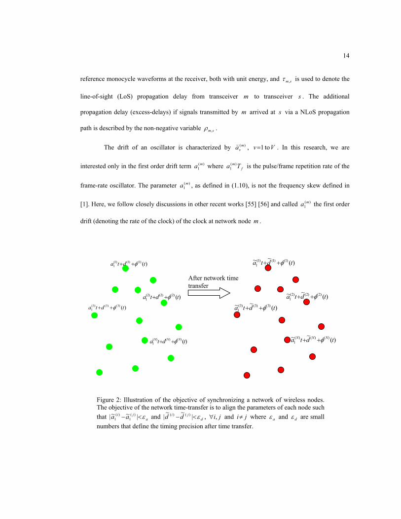
Figure 2: Illustration of the objective of synchronizing a network of wireless nodes.
14
Figure 3: System block diagram of UWB monocycle ToA measurement unit.
18
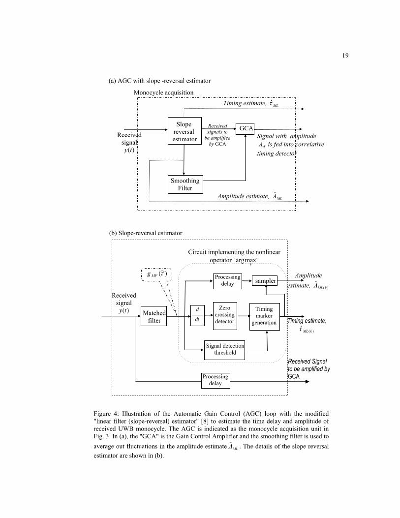
Figure 4: Illustration of the Automatic Gain Control (AGC) loop with the modified "linear filter (slope-reversal) estimator" [8] to estimate the time delay and amplitude of received UWB monocycle.
19
Figure 5: Equivalent representation of the Automatic Gain Control loop.
24
Figure 6: The variance of the amplitude estimate at the output of the matched filter estimator for effective squared bandwidth of 22 /5.8 wσω ∈ where
)2/()12( 22wn σω += and 8=n .
24
Figure 7: The mean of the amplitude detector output with 1=wA for a 8th order derivative Gaussian monocycle waveform and effective squared bandwidth
22 /5.8 wσω = .
25
Figure 8: UWB monocycles obtained in an indoor environment.
28
Table 1: The ratio )/1( 2TDg( for various values of n and 'n ( )()(),()( ' twtrtwtw nn == )
31
Figure 9: Additional variance 2MPσ due to the 2nd ray of the cluster in a multipath
propagation environment as a function of normalized quantities wσλ~ and
wσγ /~ .
38
Figure 10: Illustration of signal propagation paths between two nodes.
40
Figure 11: Illustration of estimation error by applying LS on two sets of data with different starting index STK and STK ′ where STST KK >′ .
46
Figure 12: Normalized standard deviation of Least Squares estimates for ),( smγ and ),( smζ .
48
Figure 13: A jitter-free diagram illustrating the parameters used to compute the timing offset.
50
Figure 14: Illustration of the time indices when transmitting the frame-synchronization, uplink and downlink ranging pulses for time-transfer scheme A.
53
viii
Figure 15: Illustration of the effect of differences in initial offsets and frame repetition rates between the master and slave nodes in the network.
59
Figure 16: Upper bound on the number of nodes in the network N when the difference in oscillator drift η is allows to vary assuming there is no jitter or measurement errors and K=512. The y-axis is in log scale.
60
Figure 17: Illustration of cases when there is no or multiple received monocycles per frame time at the receiver.
60
Figure 18: Illustration of the ToAs measured during the frame-synchronization, uplink and downlink time slots. In this example rs KKK == .
65
Figure 19: Illustration of the time-transfer scheme B.
66
Figure 20: Illustration of the time-transfer scheme C.
69
Figure 21: Performance of the different time-transfer schemes described in sections 3.1 and 3.4 in estimating initial offset differences.
71
Figure 22: Performance of different time-transfer schemes described in sections 3.1 and 3.4 in estimating frame-repetition-rate differences.
72
Figure 23: Flow chart illustrating the various steps taken at the slave transceiver to obtain the timing of master in the single-master time-transfer architecture.
79
Figure 24: Estimating the phase noise of the FTS9500 oscillator operating at 5 MHz.
81
Figure 25: Theoretical lower bound on the standard deviation in estimating frame frequency difference between a pair of transceivers (N=2) as a function of K for various values of φσ at received SNR of Θm,s=10 dB and Θm,s=30 dB.
82
Figure 26: Theoretical lower bound on the standard deviation in estimating difference in initial offset between a pair of transceivers (N=2) due to AWGN and oscillators' phase noise as a function of K for various values of φσ at received SNR of (a) Θm,s=10 dB and (b) Θm,s=30 dB.
83
Figure 27: Theoretical lower bound on the standard deviation in estimating difference in initial offset between a pair of transceivers due to AWGN and oscillators' phase noise as a function of N for various values of φσ at received SNR of (a) Θm,s=10 dB and (b) Θm,s=30 dB, 1000=K .
84
Figure 28:
Illustration of the "roving" master concept. 86
Figure 29: Illustration of the (a) SM, (b) HM and (c) MU time-transfer architectures. 87
Figure 30: Illustration of the time transfer activities at each node utilizing the roving master concept with time-transfer scheme A.
88
Figure 31: Illustration of the time transfer activities at each node utilizing the roving master concept with time-transfer scheme C.
89

ix
Figure 32: Illustration of the hierarchical master-slave time-transfer architecture.
90
Figure 33: Illustration of the HM time-transfer architecture for a given network topology.
92
Figure 34: Flow chart illustrating the various processes to implement a hierarchical master slave time-transfer architecture.
95
Figure 35: Flow chart illustrating the various processes to implement mutually synchronous time-transfer architecture.
97
Figure 36: Illustration of the logical channels forming the mutually synchronous SIN.
103
Figure 37: A simplified straight-line network topology to illustrate the effects of path-loss exponent on the timing error variances of SM and HM time-transfer architectures.
107
Figure 38: Normalized timing error standard deviation with path-loss exponent 2=Lρ at 30=Θ t dB and 1000=K .
108
Figure 39: Normalized timing error standard deviation with path-loss exponent 4=Lρ at 30=Θ t dB and 1000=K .
109
Figure 40: The square-root of the normalized timing sample variances when different weight functions sm,α are used in evaluating (5.12).
112
Table 2: Equations that defined the various time-transfer schemes 114
Table 3: Variances of the estimation error in estimating the differences in frame repetition rate and initial offset for SM, HM and MU time-transfer architectures
115
Table 4: Variances of timing error for SM, HM and MU time-transfer architectures
116
Figure 41: Timing error variance for a circular network topology synchronized with SM.
117
Figure 42: Illustration of the network topology used for time-transfer simulations.
124
Figure 43: Normalized standard deviation of the settled initial offset estimate for node 2 with respect to lead master node after SM, HM time transfer.
125
Figure 44: Normalized standard deviation of the settled initial offset estimate for node 17 with respect to lead master node after SM, HM time transfer.
125
Figure 45: Normalized standard deviation of the settled initial offset estimate for node 9 with respect to lead master node after SM, HM time transfer.
126
Figure 46: Normalized standard deviation of the settled timing error estimate for node 2 with respect to lead master node after SM, HM time transfer.
126
Figure 47: Normalized standard deviation of the settled timing error estimate for node 17 with respect to lead master node after SM, HM time transfer.
127

x
Figure 48: Normalized standard deviation of the settled timing error estimate for node 9 with respect to lead master node after SM, HM time transfer.
127
Figure 49: Normalized standard deviation in estimating difference in initial offset after time transfer using SM, HM and MU time-transfer architectures and time-transfer scheme A with 2=Lρ , 0=φσ and 30=Θ t dB.
128
Figure 50: Normalized standard deviation of timing error after time synchronization using SM, HM and MU time-transfer architectures and time-transfer scheme A with 2=Lρ , 0=φσ and 30=Θ t dB.
129
Figure 51: Normalized standard deviation of timing error after time synchronization using SM, HM and MU time-transfer architectures and time-transfer scheme C with 4=Lρ , 0=φσ and 30=Θ t dB.
130
Figure 52: Sample variance of network nodes' timings immediately after time-transfer using MU time-transfer architecture
131
Figure 53: Simulation results from repeatedly applying MU time-transfer to the network shown in Fig. 42 at 30=Θ t dB, 2=Lρ and 0=φσ .
132
Figure 54: Normalized timing/timing error standard deviation when co-ordinates of the network nodes are uniformly distributed and utilizing time-transfer scheme A for received SNR from 20 dB to 30 dB.
134
Figure 55: Normalized timing/timing error standard deviation when co-ordinates of the network nodes are uniformly distributed and utilizing time-transfer scheme C for received SNR from 20 dB to 30 dB.
135
Figure 56: Normalized timing/timing error standard deviation when co-ordinates of the network nodes are uniformly distributed and utilizing time-transfer scheme C for received SNR from 40 dB to 50 dB.
136
Figure 57: Illustration of the relationship between transmitter and receiver SNR.
139
Figure 58: Summary of works performed in this research.
143
Figure 59: Example of a HM time transfer architecture whereby multiple nodes formed the next tier of the hierarchy.
151
Figure 60: The nodes tree for the HM time transfer architecture shown in Figure 59.
151

xi
ABBREVIATIONS
AGC Automatic Gain Control loop
HM Hierarchical Master-slave
LS Least Squares
LoS Line-of-Sight
ML Maximum Likelihood
MU Mutually Synchronous
NLoS Non-Line-Of-Sight
PSD Power Spectral Density
SIN Synchronous Impulse Network
SM Single-Master
SNR Signal-to-Noise-Ratio
TDMA Time Divisional Multiple Access
ToA Time-of-Arrival
UWB Ultra Wideband
i.i.d. independently identically distributed
p.d.f. probability density function
p.r.r. pulse repetition rate

xii
ABSTRACT
A synchronous impulse network (SIN) is defined to be a network of spatially distributed
wireless nodes employing UWB impulse transceivers whose oscillators are "ticking" at the same
time/phase. In this research, the ultra-wide bandwidth of UWB signals is exploited to provide high
resolution timing synchronization. The network node in the proposed synchronization scheme
measures the time-of-arrival (ToA) of UWB monocycles transmitted from other nodes in the network.
The measured ToAs are impaired by additive channel noise, oscillator phase noise and may
correspond to ToA of signal arrived via non-line-of-sight (NLoS) propagation. To perform time
transfer between network nodes, the designated master node transmits frame-synchronization pulses
to slave nodes to align slaves' oscillator frame repetition rate with that of master. This is followed by
two-way ranging using the master as the transponder to mitigate signal propagation delay. This allows
a node in the SIN to estimate, from the measured ToAs, the initial offset differences between itself
and the master nodes. It is assumed that the UWB monocycles occupy all the available bandwidth and
network nodes transmit UWB impulses only in pre-assigned time slots. Thus the proposed
synchronization scheme uses only one physical channel for time transfer and logical channels are
formed via time division multiplexing. The 'roving' master concept for time transfer, whereby each
node takes a turn as the master node, is also proposed in this research. The main objective of roving
the network's nodes is to overcome blockages to network signal propagation paths and to extend the
coverage of the synchronous network. The roving masters form either the mutually synchronous
(MU) or hierarchical master-slave (HM) time transfer network architectures and their performances
are compared with a single-master time-transfer architecture (SM).

1
CHAPTER I
INTRODUCTION
1.1 Introduction
A synchronous impulse network (SIN) is defined to be a network of distributed wireless
nodes employing ultra-wideband (UWB) impulse transceivers whose oscillators are "ticking" at the
same time/phase. In this research, the ultra-wide bandwidth of UWB signals is exploited to provide
high resolution timing synchronization. It is assumed that the UWB monocycles occupy all the
available system bandwidth. Noting that the ultra-wide bandwidth makes frequency division
approaches spectrally inefficient especially when there are many nodes in the network. Therefore in
the proposed synchronization scheme, nodes in the network are allowed to transmit UWB impulses
only at pre-assigned time slots. In this setting, only one physical channel is utilized for time transfer
and logical channels are formed via time division multiplexing.
The nodes in the SIN measure the time-of-arrival (ToA) of UWB monocycles from other
nodes in the network in the presence of additive channel noise and oscillators' phase noise. The
received signal may have arrived via a non-line-of-sight (NLoS) propagation path. To perform time
transfer, the master node in the proposed synchronization scheme transmits/broadcasts frame
synchronization pulses to slave nodes to align slaves' oscillator frame repetition rate with that of
master. This is followed by two-way ranging with the master as the transponder to mitigate signal
propagation delay. By measuring the ToAs of the frame-synchronization and ranging pulses,
individual node in the SIN is able to explicitly estimate the frame frequency and initial offset
differences between its oscillator and other oscillators in the network. The estimated frame frequency
and initial offset differences are then used to correct the node's frame-rate oscillator.

2
The 'roving' master concept is devised in this research with the intention to extend the
geographical coverage of the SIN and to overcome blockages to network signal propagation paths. In
the roving master approach, each node takes a turn as the master node. The roving masters are used to
form either the mutually synchronous (MU) or hierarchical master-slave (HM) time transfer network
architectures and their performances are compared with a single-master-to-multiple-slaves time-
transfer architecture (SM). This research is envisioned primarily for transceivers with a UWB
physical layer, which has gained wide spread interest in academia and industry in recent years.
1.1.1 Motivations
The motivation of this research is to realize a synchronous impulse network (SIN) for
applications such as wireless sensor networks [15], array beam forming, reach-back communication
[23] and co-operative geo-locationing utilizing UWB impulse transceivers.
While there already exist synchronization algorithms such as those described in [5], [7], [39],
[53], [58] and a review paper, [34] to synchronize the timing of a distributed network, most of them
utilize narrowband wireless transceivers. Wireless devices utilizing ultra wide-band (UWB) impulses
for their radio interfaces are commonly believed to possess the following advantages:
(a) The narrow pulses provide fine time resolution,
(b) the UWB impulse system has the ability to resolve multipath, and therefore has less susceptibility
to fading [69] and
(c) the signal energy spreads over an ultra-wide spectrum, hence providing these signals with covert
transmission properties such as low probability of intercept and detection (LPI/LPD).
Further, it is pointed out in [58] that a propagation channel that can be characterized easily is pivotal
to good practical performance for time-transfer systems. In most channels envisioned, UWB
transceivers sending sufficiently narrow impulses do not suffer adversely from inter-pulse

3
interference, and therefore are likely to perform better than conventional carrier based continuous
narrowband systems which are often degraded by inter-symbol interference.
We are also aware of at least two concerted efforts to develop sensor networks using UWB
technology [22], [24]. One common reason cited in these commercial UWB developments is the
ability to produce UWB transceivers with small 'form factor'1. It is argued that UWB transceiver can
be build consisting of 'only a UWB transmit/receive chip, UWB antenna, digital baseband processor
and embedded firmware and protocols that drive the digital baseband processor'. As a result, fewer
components are needed compared to 'carrier based technology that must modulate and demodulate a
complex analog carrier waveform.' [http://www.pulselink.net/ov_history.html]
Unlike most recent works such as [17] and [23], which ignored signal propagation delay, this
research incorporates signal propagation time into the system model to be analyzed. Ignoring the
effect of signal propagation delay unnecessarily restricts the accuracy of time-transfer techniques. The
timing bias introduces as a result of ignoring signal propagation delay is in the order of
8103/)nodesbetweendistance( sec, which is significant relative to the width of the UWB
monocycle. For example, a signal propagation distance of 10 meters represents a delay of
30010310 8 nanoseconds. Since a UWB monocycle is typically of sub-nanosecond pulse width,
the full potential of UWB impulses to provide high timing resolution is not being fully exploited if the
effect of propagation delay is not being mitigated.
1.1.2 Network Time Transfer Approaches
Network time transfer has been a much-researched topic since the 1960s [34]. Recently, [7]
highlights the importance of network synchronization in large-scale telecommunication system
1 According to Webopedia encyclopedia on computer technology (http://www.webopedia.com/), form factor refers to the physical size and shape of a device. It is often used to describe the size of circuit boards.
4
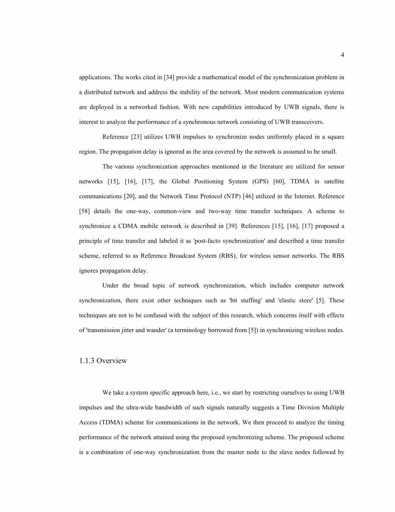
applications. The works cited in [34] provide a mathematical model of the synchronization problem in
a distributed network and address the stability of the network. Most modern communication systems
are deployed in a networked fashion. With new capabilities introduced by UWB signals, there is
interest to analyze the performance of a synchronous network consisting of UWB transceivers.
Reference [23] utilizes UWB impulses to synchronize nodes uniformly placed in a square
region. The propagation delay is ignored as the area covered by the network is assumed to be small.
The various synchronization approaches mentioned in the literature are utilized for sensor
networks [15], [16], [17], the Global Positioning System (GPS) [60], TDMA in satellite
communications [20], and the Network Time Protocol (NTP) [46] utilized in the Internet. Reference
[58] details the one-way, common-view and two-way time transfer techniques. A scheme to
synchronize a CDMA mobile network is described in [39]. References [15], [16], [17] proposed a
principle of time transfer and labeled it as 'post-facto synchronization' and described a time transfer
scheme, referred to as Reference Broadcast System (RBS), for wireless sensor networks. The RBS
ignores propagation delay.
Under the broad topic of network synchronization, which includes computer network
synchronization, there exist other techniques such as 'bit stuffing' and 'elastic store' [5]. These
techniques are not to be confused with the subject of this research, which concerns itself with effects
of 'transmission jitter and wander' (a terminology borrowed from [5]) in synchronizing wireless nodes.
1.1.3 Overview
We take a system specific approach here, i.e., we start by restricting ourselves to using UWB
impulses and the ultra-wide bandwidth of such signals naturally suggests a Time Division Multiple
Access (TDMA) scheme for communications in the network. We then proceed to analyze the timing
performance of the network attained using the proposed synchronizing scheme. The proposed scheme
is a combination of one-way synchronization from the master node to the slave nodes followed by

5
two-way ranging using the master as the transponder. In [34] and many references therein, time
transfer is performed using a phase-locked-loop to acquire the timing of the received carrier-based
narrowband signals. Here, the ToA of the transmitted monocycle at the receiver is measured
explicitly. These measured ToAs are used to derive estimates of the differences in initial offset and
frame frequency between nodes in the network. In addition, our work differs from [34] in the sense
that, besides measuring ToA explicitly, there is only one physical channel for time transfer among
nodes in the network and logical channels are formed via time division multiplexing. To the best of
our knowledge, the effect of channelization by time-multiplexing on the performance of time
synchronization has not been addressed in the open literature.
A timing detector [11] that correlates the received signal with a reference signal generated at
the receiver is used to measure the ToA. We considered four major sources of impairments to the
measurement of the ToA. They are additive noise (e.g. receiver noise), oscillator phase noise,
multipath self-interference and NLoS measurements that give a positive bias to the ToA readings [31].
For UWB impulses fully utilizing the FCC indoor spectral mask, the bias on the ToA measurements
attributed to multipath self interference is assumed negligible [12].
We seek to place a bound on the achievable timing resolution, which includes the effects of
oscillators' time drift and impairments mentioned in the previous paragraph.
Chapter 1 introduces the time function, which defines the time observed by individual
network nodes. It is followed by defining the objective of the time transfer/synchronization in this
research. Chapter 2 is devoted to measuring the relative ToA of UWB monocycles at the receiver in
the presence of additive noise and disturbances. Chapter 3 describes the proposed time
synchronization scheme to transfer clock information between a pair of network nodes. Chapter 4
extends the time synchronization scheme to synchronize a network of nodes using various network
time transfer architectures. In Chapter 5, the timing errors for different time transfer architectures are
formulated. Chapter 6 details the results and observations obtained from computer simulations of the
various network time transfer architectures and conclusions are presented in Chapter 7.

6
1.2 System Model
The system model comprises the timing function that describes the time observed by the
transceiver. Throughout this work, we assume that there exists a reference source (time standard) that
tells the 'true time' denoted by .t This allows us to describe the time observed by individual
transceiver at epoch t relative to the standard time scale [46].
The timing function of a transceiver is a function of its oscillator's initial offset, drift and
phase noise. At the same epoch ,t each transceiver will read a different time on its clock and time
intervals will be of different durations because of differences in their oscillator initial offset and drift.
There are also random timing errors between transceivers as a result of oscillator phase noise.
The received and reference signals are defined after the timing function. The reference signal
is used to correlate with the received signal to derive the timing difference between the transmitter
and the receiver. The system model is completed with a description of the nth order derivative of a
Gaussian curve, which is used to model the received UWB monocycle waveform.
1.2.1 Timing Function
It is assumed that the oscillator at each node/transceiver is described by a sinusoid of the
form
))(sin()()( ttt AY , (1.1)
where )(tA and )(t are the instantaneous amplitude and total phase function of the oscillator
respectively with variable t representing the true time. The timing function is assumed to be a
function of the oscillator instantaneous phase, and is defined as
o
ttT )()( , (1.2a)

7
where o is the oscillator's nominal frequency. The timing function (1.2a) maps the total phase of
the oscillator onto an observable time axis, i.e., the time that is observed by the transceiver. Following
[36] and [42], the imperfect timing function generated by the oscillator of transceiver m is modeled
as
)()()( )()()()( tdtatT mmmm , (1.2b)
where V
v
vmvm
vta
ta1
)()(
!)( , (1.2c)
is a function of the deterministic parameters of the oscillator and the random timing term is
o
mmm t
t)0()(
)()()(
)( . (1.2d)
The parameter )(mva characterizes the drift of the oscillator. In particular, )1( )(
1ma is known as the
normalized settability and )(2
ma the normalized drift rate of oscillator m ([42] pp. 134, 139). In [1],
)1( )(1
ma is defined as the frequency offset (or skew) and )(2
ma the frequency drift.
The random phase jitter of the oscillator2 is denoted by )()( tm . And )()( tm , in unit of
seconds, is the random timing jitter at time t . An oscillator is said to be perfect if its timing function
is given by )()( )( mm dttT .
In equations (1.2a) to (1.2d) and in subsequent analysis, the superscript in parenthesis )()( m
is used to denote transceiver m , and takes on values in the set m,s when it is used to denote a pair
of transceivers: the master 'm' and slave 's', or 1,2,3,4,…,N when denoting a particular transceiver in
a network of N transceivers. The index '1' is used to refer to the master node when more than one
slave is needed to describe the SIN. The oscillator timing function is illustrated in Fig. 1.
2 The phase jitter is also known as the oscillator's short-term instabilities and has zero mean.
8
1.2.2 Drift of Oscillator
An oscillator, being a physical device, is known to drift because of aging and external
environmental factor. The aging of an oscillator is 'the systematic change in frequency with time due
to internal changes in the oscillator'3. While the drift of an oscillator refers to 'the systematic change in
frequency with time'. The authors of [65] further state that:
3 This definition in [65] is taken from the glossary of terms and definitions (1990) of the International Radio Consultative Committee (CCIR), now known as the ITU-R.
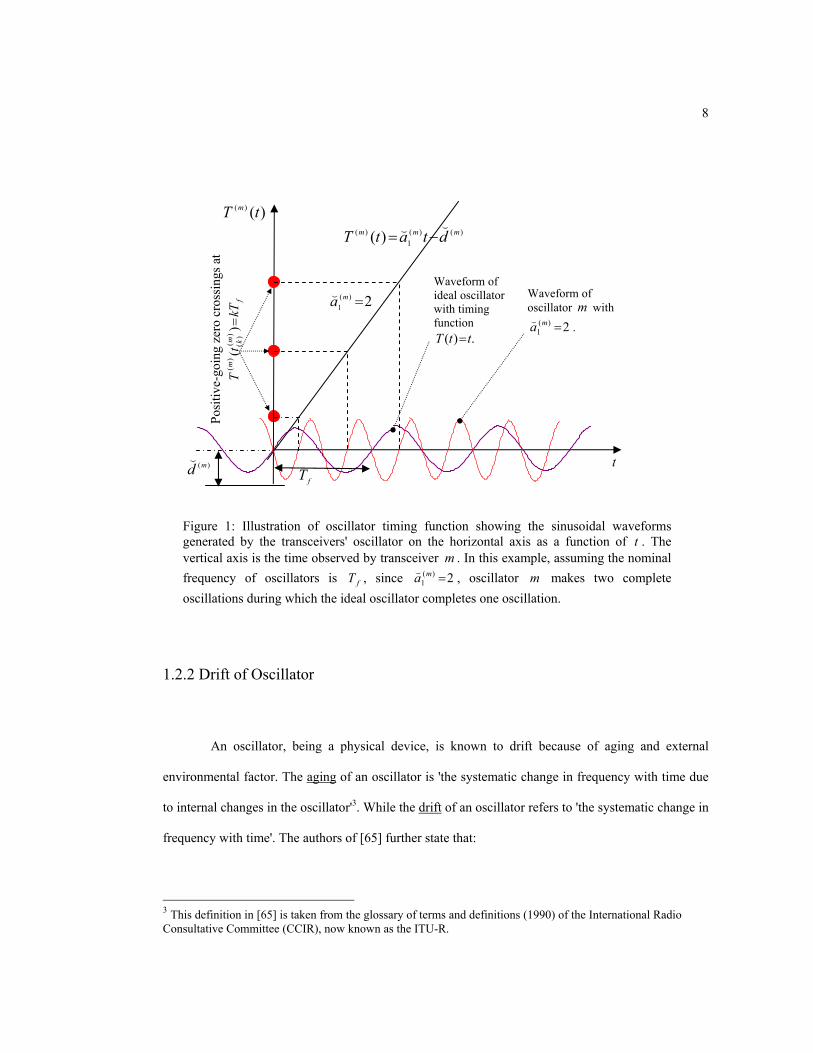
Figure 1: Illustration of oscillator timing function showing the sinusoidal waveforms generated by the transceivers' oscillator on the horizontal axis as a function of t . The vertical axis is the time observed by transceiver m . In this example, assuming the nominal frequency of oscillators is fT , since 2)(
1ma , oscillator m makes two complete
oscillations during which the ideal oscillator completes one oscillation.
Posi
tive-
goin
g ze
ro c
ross
ings
at
Waveform of ideal oscillator with timing function
.)( ttT
Waveform of oscillator m with
2)(1
ma .
)()(1
)( )( mmm dtatT
)(mdfT
2)(1
ma
)()( tT m
fm k
mkT
tT
)(
)(
)(
)(
t
9
'Drift is due to aging plus changes in the environment and other factors external to the oscillator.
Aging, not drift, is what one denotes in a specification document and what one measures during
oscillator evaluation. Drift is what one observes in an application.'
In this research, following [65], the drift of an oscillator refers to oscillator aging plus
deviations from ideal that arises from external environmental factors.
A highly accurate, precise and stable oscillator with low jitter/variance is desirable for timing
purposes. From [65], an accurate oscillator is described as one whereby its frequency of oscillation
agrees with its stated values with a high "degree of correctness". The precision of an oscillator is the
'extent to which a given set of measurements of one sample agrees with the mean of the set'. Finally,
stability describes 'the amount something changes as a function of parameters such as time,
temperature, shock, and the like'.
When a radio network requires accurately aligned clocks, it must perform time transfer
periodically to align the timing functions of different oscillators if
a) an accurate, precise and stable oscillator may not be readily available or costly, or
b) aging or environment factors may cause underlying physical properties, e.g. oscillation
frequency, of the oscillator to change.
In subsequent analysis, it is assumed that 0)(mva for 1v , m . This assumption is also
stated in the review paper [56] on time synchronization in sensor networks, and utilized in other
works [27], [39] and [55] on network time synchronization. The references [27], [39] and [56] did not
specify specific reasons for ignoring drift higher than the first order. However, in [55], it is said that
the frequency of an oscillator can be assumed to be constant for a period of time in the order of
minutes and hours. In [34], when analyzing the behavior of time synchronous network in the presence
of channel noise, a "steady" state is assumed whereby the frequency of the oscillator has a constant
time-independent mean.
From [42], the drift of oscillators due to aging is in the order of 1010 per day, while
oscillators reported in [49] have aging rate ranging from 910 to 1110 per day. Therefore if time

10
transfer is performed over a short period of time, e.g. in the order of milliseconds, it is reasonable to
assume that the frequency of the oscillator remains constant during time transfer such that 0)(mva for
1v and )(1
ma is a constant parameter to be estimated. This is similar to the steady state assumption
invoked in [34]. For this assumption to hold true, it is also necessary to assume that drift induced by
external factors, e.g. temperature changes, is not severe. Thus the network nodes are assumed to be
deployed in a benign environment that will not induce significant changes to oscillators' drift.
More about oscillator drift can be found in [49], [65] and [66]. The next section describes the
objective of time transfer.
1.2.3 Timing Error
The timing error between nodes m and s , measured at time t , at the end of time
synchronization process, is given by
)3.1(.)'()'()(
)()()()()()()()(
1)(
1
)()(),(
ttddtaa
tTtTtTsmsmsm
smsm
It is assumed that at the end of synchronization
),()(1
)(1
sma
ms aa , (1.4)
),()()( smd
ms dd , (1.5)
where ),( sma and ),( sm
d are the time transfer errors. We assume transceivers are stationary during time
transfer, as a result ),( sma is not a function of time. This allows the estimation techniques, to be
described in Chapter 3, to estimate the difference in oscillator frame repetition rate without
considering effect of time compression/expansion of signals during transmission. It is therefore
reasonable to assume that the estimation error ),( sma is a result of zero mean perturbations caused by
11
additive channel noise and oscillator phase noise and 0 ),( sma . The variance of ),( sm
a is denoted
by )( 2),(),( sma
smaV . Let
),(),(),( ~ smd
smd
smd , (1.6)
),(),( smd
smd . (1.7)
The non-zero mean 0 ),( smd is used to model the timing bias at the end of time synchronization if
the time-transfer from m to s is via an NLoS signal propagation path. The variance of the random
error ),( smd is
)8.1(.)()~(
~2),(2),(
),(),(
smd
smd
smd
smd VV
From (1.3), the mean of the timing error is
),(),( )'( smd
sm tT . (1.9a)
Since ),(),(),( )( smd
sma
sm ttT and '2)()'()( ),(),(2),(2),(2),( tttT smd
sma
smd
sma
sm , therefore
b)9.1(.'~2)()'(
')~(2)()'(
'2)()'())'((
),(),(2),(),(2),(
),(),(),(2),(),(2),(
),(),(2),(2),(2),(
tt
tt
tttT
smd
sma
smd
smd
sma
smd
smd
sma
smd
smd
sma
smd
sma
smd
sma
sm
VV
VV
V
In general, if estimates of )(1
ma and )(md are derived from the same corrupted measurements, ),( sma
and ),(~ smd may be correlated and ~~ ),(),(),(),( sm
dsm
asm
dsm
a . The timing jitter at time 't is
defined as the variance of the timing error, i.e.,
c)9.1(.'~2)'(
)'())'(()'(),(),(),(2),(
2),(2),(),(
tt
tTtTtTsm
dsm
asm
dsm
a
smsmsm
VV
V
The objective of time synchronization is to minimize )'( ),( tT smV and )'( ),( tT sm , which is
equivalent to minimizing ))'(( 2),( tT sm . These entail ensuring the differences in initial offset
)()(),( || smsmd dd and drift )(
1)(
1),( || smsm
a aa are as small as possible after time transfer.

12
1.2.4 Received and Reference Signals
Throughout this work, it is assumed that the positive-going zero crossings of an oscillator
with timing function given by (1.2b) are used to trigger the transmission of UWB impulses. That is,
UWB impulses are transmitted at times )()(
mkt that are solutions to the equation kt m
km 2)( )(
)()( for
values of k in ,...5,4,3,2,1,0 . Then )()(
mkt is written as
)10.1(,
//)/1()(
)()()(
1
)(1
)()(
)(1
)()(1
)()(
mk
mf
m
mmk
mmf
mmk
dkTa
aadkTat
where ofT /2 and for convenience, we define )(1
)(1 /1 mm aa , )(
1)()( / mmm add and
)/()(/ )(1
)(0
)()(
)(1
)()(
)()( o
mmmk
mmk
mk aa where )(
)(mk is the sampled phase noise associated with time
)()(1
)()(
mf
mmk dkTat . The pulse/frame repetition rate of the transceiver is f
m Ta )(1 .
Let 1)(1
ma and the formulations in the rest of this work do not place any restrictions on
the values of . However, nodes in the network share the same wireless channel based on TDMA.
Like any other TDMA system, it is assumed that UWB monocycles transmitted by transmitter m at
pre-assign time slots, after propagating through the wireless channel, will arrive within designated
time slots at the receiver. If the differences in pulse repetition rate and initial offset between m and s
are "too large" to begin with, this will cause monocycles to arrive at the receiver outside the
designated time slots. As a result, the proposed time-transfer scheme, to be introduced in Chapter 3,
will not perform as required.
Therefore there exist bounds on the maximum allowable differences in initial offset and drift
among all pairs of nodes in the network such that the proposed time-transfer scheme will perform as
desired. The maximum allowable differences in initial offset and drift are function of the number of
nodes in the network, signal propagation delays between nodes and the number of frames to be used
for time synchronization.
13
Thus, we assume that nodes in the network are already in some form of "coarse" time
synchronization, for example by factory setting, before deployment. Then, as stated in section 1.2.2,
the proposed synchronization scheme is applied periodically to align the timing functions of nodes in
the network or to improve the initial coarse timing synchronization to the desired accuracy.
The objective of time synchronization is illustrated in Fig. 2.
Further, with values of oscillator aging ranging from 910 to 1010 per day [42] [49], for
most practical purposes, it is reasonable to assume that 610|| .
In the subsequent analysis, it is assumed that a correlative timing detector at receiver s is
used to measure the time-of-arrival (ToA) of the received UWB monocycles. This requires a reference
signal to be generated at the receiver. Defining oscillator parameters as in (1.10), the reference
monocycles are assumed to be generated at times
)()(
)()(1
)()(
sk
sf
ssk dkTat . (1.11)
The variables )()(
mkt and )(
)(skt , measured on the standard time scale, are the kth positive-going zero-
crossing of the sinusoid generated by nodes m and s oscillators respectively. Therefore the received
and reference signals are modeled as
a)12.1(,)(
)()(
,,)(
)()()(
1
,,)(
)()(
tndkTatwA
tnttwAty
ksmsm
mk
mf
mw
ksmsm
mkw
s
b)12.1(,
)(
)()(
)()(1
)()(
)(
k
sk
sf
sr
k
skr
s
dkTatrA
ttrAtf
where ,...4,3,2,1,0k assuming one monocycle )(w per frame time fT . The reference signal
)()( tf s is correlated with the received signal to derive the timing difference between the transmitter
and receiver. The random variable )(tn is the additive noise in the channel with one-sided power
density oN , A is the amplitude of the respective signals, )(tw , )(tr are the received and the
14
reference monocycle waveforms at the receiver, both with unit energy, and sm, is used to denote the
line-of-sight (LoS) propagation delay from transceiver m to transceiver s . The additional
propagation delay (excess-delays) if signals transmitted by m arrived at s via a NLoS propagation
path is described by the non-negative variable sm, .
The drift of an oscillator is characterized by )(mva , 1v toV . In this research, we are
interested only in the first order drift term )(1
ma where fm Ta )(
1 is the pulse/frame repetition rate of the
frame-rate oscillator. The parameter )(1
ma , as defined in (1.10), is not the frequency skew defined in
[1]. Here, we follow closely discussions in other recent works [55] [56] and called )(1
ma the first order
drift (denoting the rate of the clock) of the clock at network node m .
Figure 2: Illustration of the objective of synchronizing a network of wireless nodes. The objective of the network time-transfer is to align the parameters of each node such that a
ji aa |~~| )(1
)(1 and d
ji dd |~~
| )()( , ji, and ji where a and d are small numbers that define the timing precision after time transfer.
)()1()1()1(1 tdta
)()2()2()2(1 tdta
)()()()(1 tdta NNN
)()3()3()3(1 tdta
)(~~ )1()1()1(
1 tdta
)(~~ )3()3()3(
1 tdta
)(~~ )()()(
1 tdta NNN
)(~~ )2()2()2(
1 tdta
After network time transfer

15
1.2.5 UWB Monocycle Waveform
In most instances, in order to analyze the performance of the system quantitatively, we have
to use a specific model for the received UWB monocycle. Here, the received UWB monocycle )(tw
is modelled using the nth order (n>0) derivative )(twn of the Gaussian function.
Many authors use the second derivative of a Gaussian curve to model a received UWB pulse
when evaluating radio system performance [37] [54] [70]. In this work a general formula for an nth
order derivative Gaussian monocycle is presented. The order n is taken as a design parameter and [11]
shows that the appropriate choice of n will indeed have impact on the performance of a correlative
timing detector measuring the ToA of UWB signals at the receiver.
Equations (1.13a) and (1.13b) give the time and frequency domain representations of the
UWB monocycle derived from the nth order derivative of a Gaussian curve. Here w is a scaling
factor that has unit of time (e.g., seconds) and is directly proportional to the width of the monocycle.
2/
0
24/12/24/14/12/)13(
!)!12(!)!2(2)1(!)1()(
2 n
k
knknknkptn
n nkkntpentw (1.13a)
pfnnn
cn
n efn
pifW
n
/2241
2412
!)!12()2()1(
)( . (1.13b)
In (1.13a) and (1.13b), 1ci , )2/(1 2wp and 135)...32()12(!)!12( nnn . The
monocycle waveform )(twn has the following properties:
(a) For evenn , the maximum amplitude is at t=0 and positive.
(b) For n=odd, the slope at t=0 is positive.
(c) The monocycle has unit energy, i.e., 1)(2 dttwn , and satisfies 0)(twn for wt .
The width of the monocycle is approximated by the width of the main lobe of (1.13a). If
8n , the width of )(twn is approximately w .

16
The proposed monocycle model is a function of the order of the derivative n and a scaling
factor w . Increasing the order of derivative of the Gaussian curve has the effect of shifting the
spectrum of the monocycle waveform to occupy a somewhat higher frequency range. Maintaining the
same energy per pulse, a larger scaling factor stretches the monocycle pulse wider in time and causes
a more gradual rise of the main lobe of the waveform.
17
CHAPTER II
MEASURING TIME-OF-ARRIVAL (ToA)
The time-of-arrival (ToA) of a UWB monocycle at the receiver is defined to be the time
difference between the arrivals of the UWB monocycle at the receiver relative to the start of the
receiver's frame boundary.
The proposed measurement system to measure the received signal ToA is shown in Fig. 3. It
consists of a slope reversal estimator/detector [8] embedded in a feedforward Automatic Gain Control
(AGC) loop shown in Fig. 4 respectively.
During measurement, it is assumed that the receiver's local oscillator is free running and the
output of the correlative timing detector gives the ToA of the received UWB monocycle. The local
oscillator is updated as per the time-transfer scheme to be introduced in Chapter 3.
The major sources of impairments to the measurement of the ToA considered in this research
are additive noise (e.g. receiver noise), oscillator phase noise, multipath self-interference and received
signal that arrived via NLoS propagation path that give a positive bias to the ToA readings [31]. For
UWB impulses fully utilizing the FCC indoor spectral mask, which it is assumed herewith, the bias on
the ToA measurements attributed to multipath self interference is assumed negligible [12].
This Chapter is devoted to analyzing the timing jitter at the output of the timing detector. The
results will be used later to quantify the performance of the time transfer scheme.
2.1 Acquiring UWB Monocycles
The first task involved in estimating the ToA is to coarsely measure the arrival of the
monocycle at the receiver. Reference [11] pointed out that the output of the correlative timing detector
is a function of the input signal amplitude and proposed a modified slope-reversal amplitude estimator

18
from [8] to first estimate and stabilize the amplitude of the received UWB monocycles. This task is
performed by an AGC preceding the timing detector.
Figure 3: System block diagram of UWB monocycle ToA measurement unit. By closing the appropriate switches, this unit is used to receive (a) UWB monocycles from other nodes in the network, and (b) transmit UWB monocycles when it acts as a transmitter. The solid lines are used to denote signal paths while dotted lines the control/information paths. Note that the zero-crossings of the VCO sinusoid will trigger transmission of UWB pulses (reference and transmit). The "monocycle acquisition" sub-system is illustrated in Fig. 4. The wideband signal filter is used to remove out-of-band noise from the received signal.
)( )()(
skt ttwA −
Reference monocycle generator
Monocycle acquisition
Computation, control unit
for measuring ToAs and transponding
VCO
Transmitter monocycle generator
ToA )(ˆ kMLτ & Amplitude )(ˆ
kMLA estimates
(a)
(b)
Initial offset and drift
difference estimates
)(kx KD ∫
kTf
Correlative Timing Detector
Signal Processing
(e.g. LS estimator)
VCO
)()()( ,,)(
)( tnttwAtyk
smsmmkw +−−−= ∑ ρτ
free running
Wideband
Signal filter
∑ −=k
skr ttrAtf )()( )(
)(
w
d
A
Aty ˆ)( ⋅
19
(a) AGC with slope -reversal estimator
Slope reversal estimator
GCA
Monocycle acquisitionTiming estimate, MLτ
Received signals to
be amplified by GCA
Signal with amplitude dA is fed into correlative
timing detector
Amplitude estimate, MLA
Smoothing Filter
Received signal
)(ty
Figure 4: Illustration of the Automatic Gain Control (AGC) loop with the modified "linear filter (slope-reversal) estimator" [8] to estimate the time delay and amplitude of received UWB monocycle. The AGC is indicated as the monocycle acquisition unit in Fig. 3. In (a), the "GCA" is the Gain Control Amplifier and the smoothing filter is used to average out fluctuations in the amplitude estimate MLA . The details of the slope reversal estimator are shown in (b).
Circuit implementing the nonlinear operator 'maxarg'
τ
Zero crossingdetector
Signal detectionthreshold
Timing marker
generation
Processing delay
Amplitude estimate, )(
ˆkMLA
Timing estimate,
)(ˆ kMLτ
d
dt Matched
filter
sampler
Received Signal to be amplified by GCA
(b) Slope-reversal estimator
Received signal
)(ty
)~(τMFg
Processing delay
20
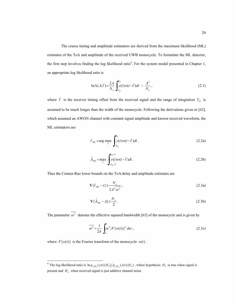
The coarse timing and amplitude estimators are derived from the maximum likelihood (ML)
estimates of the ToA and amplitude of the received UWB monocycle. To formulate the ML detector,
the first step involves finding the log likelihood ratio4. For the system model presented in Chapter 1,
an appropriate log likelihood ratio is
o
T
To NAdttwty
NAA
D
D
2
)~()(2)~,(ln −−=Λ ∫− ττ , (2.1)
where τ~ is the receiver timing offset from the received signal and the range of integration DT is
assumed to be much longer than the width of the monocycle. Following the derivations given in [62],
which assumed an AWGN channel with constant signal amplitude and known received waveform, the
ML estimators are
∫− −=D
D
T
TML dttwty )~()(maxargˆ
~ τττ
. (2.2a)
∫+
+−
−=τ
ττ
τ
~
~~ )~()(maxˆ
D
D
T
TML dttwtyA . (2.2b)
Thus the Cramer-Rao lower bounds on the ToA/delay and amplitude estimates are
222ˆ
ωττ
A
N oML ≥−V , (2.3a)
2
ˆ oML
NAA ≥−V . (2.3b)
The parameter 2ω denotes the effective squared bandwidth [63] of the monocycle and is given by
∫∞
−∞
= ωωπ
ω dtwF 222 |)(|21 , (2.3c)
where )( twF is the Fourier transform of the monocycle )(tw .
4 The log-likelihood ratio is )|)(()|)((ln |1| 1 oHyHy HtypHtyp
o, where hypothesis 1H is true when signal is
present and oH when received signal is just additive channel noise.
21
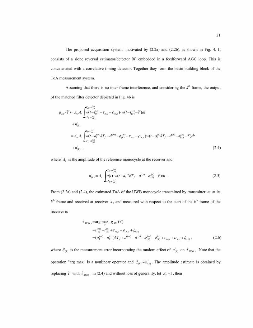
The proposed acquisition system, motivated by (2.2a) and (2.2b), is shown in Fig. 4. It
consists of a slope reversal estimator/detector [8] embedded in a feedforward AGC loop. This is
concatenated with a correlative timing detector. Together they form the basic building block of the
ToA measurement system.
Assuming that there is no inter-frame interference, and considering the kth frame, the output
of the matched filter detector depicted in Fig. 4b is
)4.2(,
)~()(
)~()()~(
/)(
)()(
)()(1,,
)()(
)()(1
/)(
)()(,,
)()(
)()(
)()(
)()(
)()(
k
tT
tT
sk
sf
ssmsm
mk
mf
mrw
k
tT
tT
sksmsm
mkrwMF
n
dtdkTatwdkTatwAA
n
dtttwttwAAg
skD
skD
skD
skD
+
−−−−−−−−−=
+
−−⋅−−−=
∫
∫+
+−
+
+−
τφρτφ
τρττ
where rA is the amplitude of the reference monocycle at the receiver and
∫+
+−
−−−−⋅=
)()(
)()(
)~()( )()(
)()(1
/)(
skD
skD
tT
tT
sk
sf
srk dtdkTatwtnAn τφ . (2.5)
From (2.2a) and (2.4), the estimated ToA of the UWB monocycle transmitted by transmitter m at its
kth frame and received at receiver s , and measured with respect to the start of the kth frame of the
receiver is
)6.2(,)(
)~(maxargˆ
)(,,)()(
)()(
)()()(1
)(1
)(,,)()(
)()(
~)(
ksmsmsk
mk
smf
sm
ksmsmsk
mk
MFkML
ddkTaa
tt
g
ξρτφφ
ξρτ
τττ
+++−+−+−=
+++−=
=
where )(kξ is the measurement error incorporating the random effect of /)(kn on )(ˆ kMLτ . Note that the
operation "arg max" is a nonlinear operator and /)()( kk n≠ξ . The amplitude estimate is obtained by
replacing τ~ with )(ˆ kMLτ in (2.4) and without loss of generality, let 1=rA , then

22
)7.2(.)()(
)ˆ()(
)ˆ()(
)ˆ()~(maxˆ
/)()(
/)(
)()()(
)()(1,,
)()(
)()(1
/)()(
)()(,,
)()(
)(~)(
,,)(
)()()(
,,)(
)()()(
)()(
)()(
)()(
)()(
k
ttT
ttTkw
k
tT
tTkML
sk
sf
ssmsm
mk
mf
mw
k
tT
tTkML
sksmsm
mkw
kMLMFMFkML
ndttwtwA
n
dtdkTatwdkTatwA
ndtttwttwA
ggA
smsmmk
skD
smsmmk
skD
skD
skD
skD
skD
+−=
+
−−−−−−−−−=
+−−−−−=
==
∫
∫∫
−−−+
−−−+−
+
+−
+
+−
ρτ
ρτ
τ
ξ
τφρτφ
τρτ
ττ
Equations (2.4) to (2.7) assume that there is only one monocycle per frame. Also, the monocycle
transmitted at the kth frame of transmitter m is received at the kth frame of receiver s .
2.2 Automatic Gain Control Loop
A feedforward AGC is chosen for its stability with minimum time lag between its input and
output. For the purpose of this analysis, the AGC of Fig. 4a is represented in Fig. 5 using its
equivalent model. From (2.7), the output of the amplitude detector is denoted by )(ˆ
kMLA . Following
the derivations given in [42], the amplitude suppression factor of the detector is defined as the ratio of
the estimated amplitude to the input signal amplitude and denoted by )( )(kSF ξΛ . It is assumed that
the amplitude of the received monocycle remains stable during measurement, then
a)8.2(,)(
|)ˆ(
|ˆ)(
)(
)()(
)()()(
Ε
Ε
k
w
kkMLMF
w
kkMLkSF
Ag
AA
ξ
ξτ
ξξ
Ψ=
=
=Λ
∫−−+
−−+−
−=Ψsm
mk
skD
smmk
skD
ttT
ttTkk dttwtw
,)(
)()()(
,)(
)()()(
)()()( )()(
τ
τ
ξξ , (2.8b) where

23
which is the auto-correlation function of the UWB monocycle pulse )(tw . This allows us to express
the output of the amplitude detector )(ˆ
kMLA as
/)()()( )(ˆ
kkSFwkML nAA +Λ⋅= ξ . (2.9)
The random variables )(kξ and /)(kn are not independent, and in general )(kξ is a function of signal-to-
noise-ratio (SNR, defined as )2//(2oNA ). In this work, no further attempt is make to examine the
statistical properties of )(ˆ
kMLA analytically.
The Gain Control Amplifier (AGC) depicted in Fig. 5 is a device that amplifies the signal at
its input. From [42], we know that there are various possible characterizations of the GCA depending
on the actual devices that are being utilized. Here it is assumed that a GCA with a hyperbolic gain is
used. The characteristic function of the hyperbolic GCA is
)()( )ˆ,(
kML
dkMLd A
AAAG = , (2.10)
where dA is the desired signal amplitude. Thus, the amplitude of the signal at the output of the
feedforward AGC becomes
)11.2(.)(
ˆ
)ˆ,(
/)()(
)(
)()(
kwkSF
wd
kML
wd
wkMLdko
nAAA
A
AA
AAAGA
+⋅Λ=
=
⋅=
ξ
If 0/)( →kn , 0)( →kξ 1)( )( →Λ⇒ kSF ξ , wkML AA ≈)(
ˆ and do AA = . Some form of averaging can be
implemented at the output of the AGC to average out fluctuations in )(koA .
The linear slope reversal amplitude estimator depicted in Fig. 4b is simulated and the results
plotted in Figs. 6 and 7 for received SNR ( )2//(2ow NA ) from 10 to 30 dB. In the simulation, to find
)(ˆ
kMLA , the matched filter output )~(τMFg is searched over a range of -2000Ts to 2000Ts centered at

24
the actual ToA position, where Ts is the sampling period of the simulation. The error in estimating the
signal amplitude is negligible for most practical purposes for received SNR above 15 dB.
The estimated delay )(ˆ kMLτ from the matched filter and the received UWB monocycle at the
output of the AGC are then processed by the correlative timing detector.
1.E-04
1.E-03
1.E-02
1.E-01
15 17 19 21 23 25 27 29
Figure 6: The variance of the amplitude estimate at the output of the matched filter estimator for effective squared bandwidth of 22 /5.8 wσω ∈ where )2/()12( 22
wn σω += and 8=n . The sampling period is 0.01 wσ and 1=wA . The theoretical bound is given by (2.3b).
SNR )2//(2ow NA= dB
Theoretical bound Simulated
)ˆ
(2
)(k
ML
wA
A−
Ε
Figure 5: Equivalent representation of the Automatic Gain Control loop. The parameter GD is the gain of the amplitude detector. Without loss of generality, GD is set to 1.
)(ˆ
kMLD AG ⋅
/)(kn SFΛ
GCA
delay
GD wA
oA
)ˆ,( )(kMLd AAG
Amplitude detector
dA
25
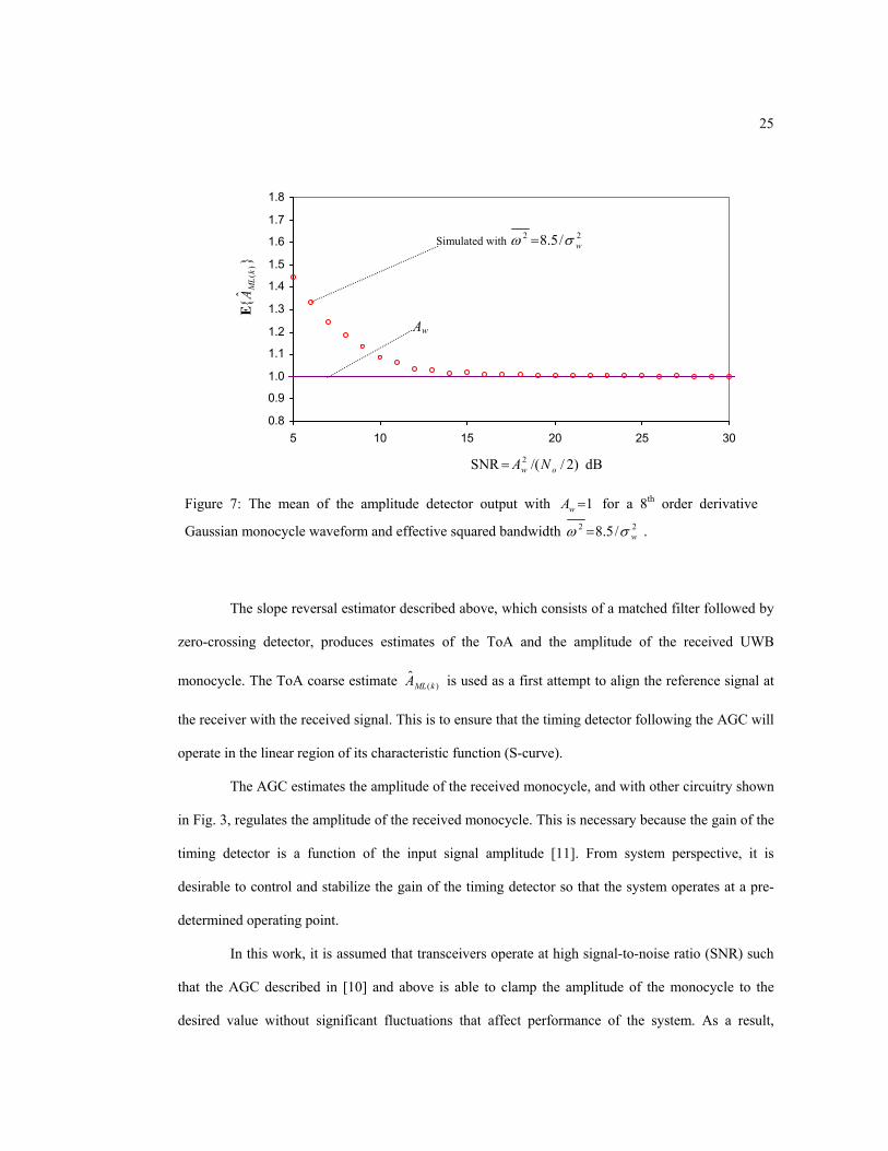
The slope reversal estimator described above, which consists of a matched filter followed by
zero-crossing detector, produces estimates of the ToA and the amplitude of the received UWB
monocycle. The ToA coarse estimate )(ˆ
kMLA is used as a first attempt to align the reference signal at
the receiver with the received signal. This is to ensure that the timing detector following the AGC will
operate in the linear region of its characteristic function (S-curve).
The AGC estimates the amplitude of the received monocycle, and with other circuitry shown
in Fig. 3, regulates the amplitude of the received monocycle. This is necessary because the gain of the
timing detector is a function of the input signal amplitude [11]. From system perspective, it is
desirable to control and stabilize the gain of the timing detector so that the system operates at a pre-
determined operating point.
In this work, it is assumed that transceivers operate at high signal-to-noise ratio (SNR) such
that the AGC described in [10] and above is able to clamp the amplitude of the monocycle to the
desired value without significant fluctuations that affect performance of the system. As a result,
Figure 7: The mean of the amplitude detector output with 1=wA for a 8th order derivative
Gaussian monocycle waveform and effective squared bandwidth 22 /5.8 wσω = .
0.8
0.9
1.0
1.1
1.2
1.3
1.4
1.5
1.6
1.7
1.8
5 10 15 20 25 30
SNR )2//(2ow NA= dB
Simulated with 22 /5.8 wσω =
Aw
ˆ
)
(kM
LA
Ε

26
wkML AA ≈)(ˆ and dko AA =)( , and the correlative timing detector that follows the AGC will be able to
lock onto the received UWB monocycle. Otherwise, considerably more complicated analysis is
needed to analyze the performance of the system considering phenomenon such as detector mean-
time-to-lose-lock or detector operates on the nonlinear region of its characteristic function.
2.3 Correlative Timing Detector
The characteristic function (S-curve) of the correlative timing detector is given by [11]
∫∞
∞−
+= dttrtwAAg rko )()()( )( ςς , (2.12)
where )(tr is the reference monocycle generated at the receiver and ς is the timing error between the
received and reference signal.
The estimate )(ˆ kMLτ is used to bring the reference signal near to the peak of the received
monocycle so that ς , assuming ς has a small magnitude, fluctuates about the stable equilibrium
point at 0=ς . This allows us to approximate5 )(ςg by ( )0|)/)(()( =⋅= ςςςςς ddgg around 0=ς . Thus
)(ˆ kMLτ adjusts the correlative timing detector so that it operates within the linear region of its
characteristic function.
From Fig. 3, at the thk frame, the output of the correlative timing detector is
//)()()( )( kDkDk nKgKx ⋅+⋅= ς , (2.13)
where
∫+
+−
+=
)()(
)()(
)()()( )()()(
skD
skD
tT
tT
krkok dttrtwAAg ςς , (2.14a)
5 This approximation is widely known as the tracking/linearity assumption.
27
)()(
//)( ˆ k
kML
rdk n
A
AAn = , (2.14b)
∫∞
∞−
+= dttrtnn kk )()( )()( ς . (2.14c)
and the factor DK is the detector gain. The coefficient in front of )(kn in //)(kn of (2.14b) arises from
multiplying the received signal )(ty by )(ˆ/ kMLd AA after passing the received signal through the AGC.
Let TDg( be the slope of the characteristic function of the timing detector evaluated at 0=ς , i.e.,
d)14.2(.)()(
)(
0
0
=
∞
∞−
=
∫ +=
=
ς
ς
ςς
ςς
dttrtwdd
ddg
gTD(
Applying the linearity/tracking assumption, the characteristic function becomes
)()()( )( kTDrkok gAAg ςς ⋅⋅= ( . (2.15)
In the subsequent analysis, the reference monocycle amplitude is set to unity, i.e., 1=rA . Without loss
of generality, DK is chosen to make the slope of the detector characteristic to be 1. However in the
absence of perfect knowledge of the received signal amplitude, the receiver assumes that it is dA , i.e.,
the desired signal amplitude. Therefore, the detector gain is set at
dTDD Ag
K (1
= . (2.16)
As illustrated earlier, for SNR above 15dB, the amplitude detector is able to estimate the
amplitude of the received signal accurately, i.e., wkML AA ≈)(ˆ .
In this work, we assumed that the received SNR is above 15 dB. As a result, the amplitude
of the received signal after passing through the AGC is approximated by dko AA =)( . Moreover, the
noise term //)(kn reduces to wkd AnA /)( and the output of the timing detector can now be written as

28
)17.2(.
1
)(
)()(
)()(
)()(
)()()(
wTD
kk
w
kd
TDdk
w
kdDkTDdD
w
kdDkDk
Agn
AnA
gA
AnA
KgAK
AnA
KgKx
⋅+=
⋅⋅
+=
⋅+⋅⋅⋅=
+⋅=
(
(
(
ς
ς
ς
ς
The variable )(kς is the timing difference between the received UWB signals and the locally
generated reference signals. From the system model presented in Chapter 1, equations (1.12a) and
(1.12b), )(kς is corrupted by the transmitter and receiver oscillators' phase noise )(kφ .
In Fig. 8, examples of received UWB monocycles measured in an indoor environment are
shown. In subsequent sections, we deal with the effect of individual impairments on the output of the
timing detector when the detector is measuring the ToA of UWB monocycles.
Figure 8: UWB monocycles obtained in an indoor environment. (a) Transmitter and receiver are facing each other (LoS signal). (b) The transmitted signal propagates through a wall before reaching the receiver. (The measurements were taken in a UWB reciprocity experiment conducted with Robert Wilson of CSI, USC.)
0.0E+00 2.0E-09 4.0E-09 6.0E-09 8.0E-09 1.0E-08 1.2E-08
0.0E+00 5.0E-09 1.0E-08 1.5E-08 2.0E-08 2.5E-08
(a)
(b)
Time (secs)
Time (secs)
Am
plitu
de
Am
plitu
de

29
2.3.1 Effect of Additive Channel Noise
The AWGN in the channel contributes to timing jitter at the output of the timing detector. In
(2.17), given )(kς , i.e., ignoring the effect of oscillators' phase noise and treating )(kς as a
deterministic variable, the variance of the timing detector output is given by
=2
2)(
)()( )(|
TDw
kkk gA
nx (ΕV ς , (2.18)
where 2/ 2)( ok Nn =Ε and TDg( is given by (2.14d).
The slope TDg( contains all dependence of | )(2
)( kkx ςV on )(tw and )(tr and is a measure
of the magnitude of the slope of the S-curve at 0=ς . Clearly, to minimize the effect of the input noise
on the timing error variance, the task is to maximize the ratio / 2)(
22kTDw ngA Ε( . However, given the
received signal amplitude wA and the noise variance in the channel 2)(knΕ , it is equivalent to
maximizing 2TDg( subject to the constraints that )(tw and )(tr of (2.14d) are both of unit energy, i.e.,
1)(2 =∫∞
∞−
dttr and 1)(2 =∫∞
∞−
dttw .
To place a bound on )(kxV , the quantity 2TDg( is expressed as
[ ]∫∫∞
−∞=
∞
−∞
=+ dfffFifFdttrtwdd C
rcw )(2)()()(0
πςς ς
, (2.19)
where [ ]CfR )( denotes the complex conjugate of )( fR and )( fFr the Fourier transform of )(tr .
Let [ ]∫ ⋅= dttytxyx C)()(, be the usual inner product space in ),(2 ∞−∞L . We denote a bounded
linear operator on a Hilbert space as Κ and its adjoint *Κ such that >Κ>=<Κ< yxyx ,*, . Here, these
linear operators on )( fFr can be written as6
6 The operator K* is shown to be unique in [47].

30
[ ]
→Κ⋅→Κ
)(2)(:*)(2)(:
fFfifFfFfifF
xcx
xC
cx
ππ . (2.20)
Applying the Schwartz inequality to (2.19), we obtain
a)21.2(.)()(
)(),(
)(*),(
22
2
22
fFfF
fFfF
fFfFg
rw
rw
rwTD
Κ≤
Κ=
Κ=(
Equality occurs when )(2)( fFfifF wcr π−∝ or dttdwtr /)()( −∝ . Thus the optimal reference signal
is the time derivative of the received monocycle waveform. In [11], it is derived that
22 ω=TDg( , (2.21b)
when dttdwtr /)()( = . Since 2TDg( is upper bounded by 2ω (2.21a), )(kxV of (2.18) is lower
bounded by7
2,
)()(1|ω
ςsm
kkxΘ
≥V , (2.22)
where owsm NA2, 2=Θ is defined as the received SNR at the receiver. It can be shown that
22222)( ))()(()( ∫
∞
∞−+⋅⋅⋅⋅= dttrtwAAKx rwDk ςΕ and ∫
∞
∞−+⋅⋅⋅= dttrNAKx orDk )()2/()| 222
)( ςςV . If
0=ς , )()( twtr = , since 1)(2 =∫∞
∞−dttw , then the ratio smowkk NAxx ,
2)(
2)( /2|/)( Θ==ςVΕ . For
simplicity in notation, the term ∫∞
∞−dttw )(2 is not carried around in subsequent analysis and sm,Θ
should be understood as a unit-less quantity.
The lower bound in (2.22) is known as the Cramer-Rao bound on estimating the non-random
delay of a signal distorted by additive noise in the channel [43] [63]. This bound is derived with no
restriction on the bandwidth of the signal. We note that this bound is optimistic because matched filter
UWB receivers are hard to build.
7 This result has been arrived at using different techniques in different contexts [48] [50] [68].

31
Utilizing the monocycle waveform (derivative of a Gaussian curve) defined in Chapter 1,
equations (1.13a) and (1.13b), if )()( twtw n= and )()( ' twtr n= are substituted into (2.19), the slope at
0=ς is [11]
=++
−−
+−
=+=
∞
∞−∫
otherwise
evennnifnn
nnpdttwtw
dd n
nn
0
1'!)!1'2(!)!12(
!)!'()1()()(
0'
ς
ςς
. (2.23)
It can be shown that in the optimal case when 1' +=nn , we have for n even [11],
)24.2(,)12(
)()(2
0'
2
pn
dttwtwdd
nn
+=
+=
=
∞
∞−∫
ς
ςς
ω
with unit sec-2. In table 1, 2/1 TDg( is tabulated for various values of n and 'n . It indicates that a UWB
monocycle waveform that is of a higher order derivative of the Gaussian curve is desirable if the
objective is to reduce the timing error variance due to AWGN at the input of the detector. The
improvement when raising the order from (n=2,n'=3) to (n=10,n'=11) is as high as 6.23 dB. It seems
that a higher order Gaussian monocycle has a main lobe that rises faster than a lower order pulse
which contributes to this gain.
Table 1: The ratio )/1( 2TDg( for various values of n and 'n ( )()(),()( ' twtrtwtw nn == )
n'=2 3 4 5 6 7 8 9
n=2 - )5/(1 p - )35/(9 p - )315/(143 p - )231/(221 p
3 p/20.0 - )7/(1 p - )63/(11 p - )231/(65 p -
4 - p/14.0≈ - )9/(1 p - )99/(13 p - )429/(85 p
5 p/26.0≈ - p/11.0≈ - )11/(1 p - )143/(15 p -
6 - p/17.0≈ - p/09.0≈ - )13/(1 p - )195/(17 p
7 p/45.0≈ - p/13.0≈ - p/08.0≈ - )15/(1 p -
8 - p/28.0≈ - p/10.0≈ - p/06.0≈ - )17/(1 p
9 p/957.0≈ - p/198.0≈ - p/087.0≈ - p/059.0≈ -

32
2.3.2 Effect of Oscillator Phase Noise
In this work, it is assumed that there is no movement of the network nodes during time
transfer, then the short-term fluctuations in )(kx of (2.17) are only due to randomness in )(kς and
additive noise in the channel. The random variable )(kς is the timing difference between the received
UWB signal and the locally generated reference signal. From the system model presented in Chapter
1, randomness in )(kς is caused by the random variables )()(
mkφ and )(
)(skφ , which are related to the
oscillator phase noise )(tϕ through (1.2d).
From [42], the oscillator phase noise )(tϕ with power spectral density )(ωϕS can be
quantified using the first structure function )(1 ∆ϕD of the phase noise process
( ) a)25.2(,)()/2()(2/sin)/2(
)()()(
2
21
Ε
∫∫∞
−∞
∞
−∞
≤∆=
−∆+=∆
ωωπωωωπ
ϕϕ
ϕϕ
ϕ
dSdS
ttD
where ∆ is the time interval of interest, e.g., the nominal pulse repetition period fT . In (2.25a), we
have made used of the fact that 1)2/(sin 2 ≤∆ω . Further, the timing jitter due to )(kφ is defined as
212 /)( oD ωσ ϕφ ∆= . (2.25b)
More details on characterizing the oscillator phase instabilities using structure functions can
be found in [35]. Reference [35] points out that the first structure function )(1 ∆ϕD of the phase noise
characterizes the stability of the oscillator phase. As put forth in [35], )(tϕ is not stationary
(increments of )(tϕ can be stationary) and thus does not possess a power spectral density (PSD) in
the usual sense. To circumstance this difficulty, [35] defined 2/)()( ωωω ϕϕ &SS = where
dttdt /)()( ϕϕ =& and )(tϕ& is a stationary, zero mean random process. The same definition is adopted
herein.
33
2.3.3 Effect of Multipath Self-Interference
(a) Multi-path Channel Model
The UWB multi-path channel model is adopted from the modified Saleh-Valenzuela (SV)
model described by the IEEE 802.15 working group [19]. It describes a UWB multipath channel
consisting of clusters of "rays" arriving at the receiver. The channel impulse response consists of
Dirac delta functions spaced according to the inter-rays arrival time within the cluster. In addition, the
amplitude of the transmitted signal is attenuated by an exponential factor. This discrete time channel
impulse response is of the form
∑ ∑= =
−−⋅=h
h
h
hhhhhh
L
l
K
k,lkl,lk τTtδχth
0 0)~~(~)( α , (2.26)
where χ represents log-normal shadowing, hh ,lkα
~ is the multipath gain coefficient, hl
T~ is the delay of
the th)( hl cluster and hh ,lkτ~ the delay of the th)( hk multipath component relative to the th)( hl cluster
arrival time. The cluster and ray arrival rate are Λ~ and λ~ respectively. The inter-arrival times of the
cluster and rays within each cluster are modelled using exponential distributions. Specifically, the
conditional probability density function (p.d.f.) on hh ,lkτ~ is
)~~(1
1~)~~( h,lhkh,lhk
hhhh
ττλ,lk,lk eλτ|τ −−−
− ⋅=P , 0>hk . (2.27a)
If 0=hk , by definition, 0~,0 =
hlτ . The channel coefficients in (2.26) are given by
hhhhhhh ,lkl,lk,lk βξα~~~~ ⋅⋅=υ . (2.27b)
Signal inversion due to reflections is modelled via hh ,lkυ
~ , which is distributed equi-probably over ±1.
The factors hl
ξ~ and
hh,lkβ~ denotes fading associated with the th)( hl cluster and the th)( hk ray of the
th)( hl cluster respectively. It is further assumed in [19] that
34
γ/τΓ/To,lkl
h,lhkhl
hhheeβξ
~~~~2 ~~~ −−Ω=
Ε , (2.27c)
where oΩ~ is the mean energy of the first path of the first cluster. The cluster and ray attenuation
factors are denoted by Γ~ and γ~ respectively.
(b) Variance of Multipath Self-interference
In this section, the effect of multipath self-interference on the performance of the open loop
timing detector is analyzed. The received signal at the input to the timing detector is written as
)()~~(~)(~ tnτTtwαχAtyh h
hhhhhl k
,lkl,lkt +−−= ∑∑ , (2.28)
where )(tn is the additive noise in the channel with one-sided PSD of oN and tA is the amplitude of
the transmitted monocycle. The output of the detector, in the absence of noise, becomes
.)()~~(~)( ∑ ∑ ∫∞
∞−
+−−⋅=⋅h h
hhhhhl k
,lkl,lkrwDD dttrτTtwαAχAKgK ςς (2.29a)
Equation (2.29a) indicates that the output of the correlative timing detector is corrupted by multipaths
in the channel.
In this work, it is assumed that the ToA is derived from the first ray of the first multipath
cluster, i.e., in subsequent analysis, 1=hl . Further, while tracking the first ray of the 1=hl multipath
cluster, the contributions to the timing detector output from multipath rays originated from other
clusters are ignored. The timing detector output reduces to
.)()~~(~)( 11∑ ∫∞
∞−
+−−=⋅h
hhhk
,k,lkrwDD dttrτTtwαAχAKgK ςς (2.29b)
As pointed out in section 2.3, the gain of the timing detector is a function of the received
signal amplitude and an Automatic Gain Controller (AGC) is placed before the correlative timing
detector to ensure constant detector gain. From (2.17), the output of the timing detector is
35
.)( )()()(
wTD
kkDk Ag
ngKx
⋅+⋅= (ς (2.30a)
where )/(1 dTDD AgK ⋅= ( and 10~
,tw AA αχ ⋅⋅= is the amplitude of the first ray of the first multipath
cluster. Assuming that there is enough SNR such that the amplitude of the monocycles at the output of
the AGC is dko AA =)( and wkML AA =)(ˆ . The output of the timing detector becomes
b)(2.30,)()~(~~
)()(1
)~()~(~~
)~()(1
)()~~(~)()~(~~
1
)(
11
1,0
1,
)(
111
1,0
1,1
)(
1111,1,0
,0)(
wTD
k
k,k
k
TD
wTD
k
k,k
k
TD
wTD
k
k,kkl
l
d
TDdk
Agn
dttrτtwdttrtwg
Agn
dtTtrτtwdtTtrtwg
Agn
dttrτTtwdttrTtwA
gAx
hh
h
hh
h
hhhh
h
⋅+
′+−⋅+′+⋅=
⋅+
++−⋅+++⋅=
⋅+
+−−⋅++−⋅⋅
⋅=
∑ ∫∫
∑ ∫∫
∑ ∫∫
≠
∞
∞−
∞
∞−
≠
∞
∞−
∞
∞−
≠
∞
∞−
∞
∞−
((
((
((
ςα
ας
ςα
ας
ςαςαα
where 1~T+=′ ςς .
In the modified SV channel model for UWB systems [19], the signal inversion coefficient
hh ,lkυ~ is statistically independent and has zero mean. As a result, 0~ , =
hh lkαΕ and
0)( =⋅ ςgK DΕ . (2.31)
In (2.31), )(ςg is a function of the channel coefficients, and is described statistically by (2.27b) and
(2.27c). Assuming that the multipath components have independent random amplitudes, the variance
of the sum of (2.30b) is the sum of the variances. Therefore the variance of the detector output,
conditioned on 1~T and 1,
~hkτ , is computed as
)32.2(.)()~(1
2~)()(1
0
2
1,
~~
2
22
~~2
22
)(
1,
1
∑ ∫
∫
≠
∞
∞−
−
∞
∞−
′+−+
⋅
Ω⋅⋅+
′+⋅=
hh
hk
kk
TD
o
ot
ΓT
TDk
dttrtweg
NA
edttrtwg
x
ςτ
χς
γτ(
( ΕΕ
The variance expressed by (2.32) consists of two separate parts: variance of the first ray corrupted by
AWGN and the variance attributed to self-interference from the multipath components.

36
In the presence of additive noise, measuring the first ray of the cluster requires sufficient
received signal energy for tolerable timing error jitter. This is described by the Cramer-Rao (CR)
lower bound of (2.22).
To justify ignoring multipath rays from other clusters, considered a signal arrives via a NLoS
path 10 nanoseconds after the first ray of the th)( hl cluster, i.e., 10~1 ≈+hl
T nano-secs, which represents
a difference in signal propagation distance of 3 meters, and if 1.7~=Γ as in IEEE 802.15.3a report,
ΓT hle~/~
1+− represents a reduction in power of 6.1 dB ))log(10( 1.7/10−= e compared to the first ray of the
th)( hl cluster. The effect of a multipath component from another cluster therefore, on average, is of
6.1 dB less power than the signal to be tracked. With this 6.1dB reduction of power, it is assumed that
multipaths from other clusters contribute negligibly to the timing detector output.
In subsequent analysis, let )()( twtw n= and )()( ' twtr n= . Making use of the Parseval's
relationship and the integral solutions in ([2], equation 7.3.1) ([21], equation 3.462), we arrive at
!)!1'2(!)!12()!'()1()()~(
2/~2/)'('
'1,
2
−−
+−=′+−
−++∞
∞−∫
nnepnndttwtw
pnnnn
nkn h
ζ
ςτ ∑+
=
−+
−+−2/')(
0
2'
)2(!)!2'(
~)1(nn
kk
knnk
pkknnζ , (2.33)
where 1,~~
hkτςζ +′= . If there is no multipath components and no timing error between the received
signal and the reference signal at the receiver, i.e., 0~1, =hkτ and 0=ς , because )'( nn+ is designed to
be odd, (2.33) is identically zero.
Let V~ be the right-hand-side of (2.33), then
( )⋅
−−+⋅
=+
!)!1'2(!)!12()!'(~ 2'
2
nnnnp
Vnn
−+−∑
+
=
−+−
2/)(
011
11
1212
)2(!)!2()1(mn
vv
vmnvp
pvvmne ττ
−+−
∑+
=
−+2/')(
0 22
2'
22
22
)2(!)!2'()1(nn
vv
vnnv
pvvnnτ . (2.34)
An analytical expression for the variance due to the second ray in the cluster is presented
next. We postulate that, because of the narrow pulse width of UWB impulses, it is sufficient for most
applications to consider only the additional variance caused by the second ray of the cluster if the
objective of the timing detector is to measure the ToA of the first ray of the cluster. The conditional

37
p.d.f. of the second ray of the cluster is 1,1~~
1,.01,1~)0~|~( τλλττ ⋅−⋅== eP . Therefore the variance at the output
of the timing detector due to the second ray in the first cluster is
γτσ~/~222 1,1~)/1( −⋅= eVgTDMP Ε( . (2.35a)
Substituting (2.34) into (2.35a), leads to
( )!)!1'2(!)!12(2
)!'(~)/1(1'
22/122
−−+⋅⋅
= ++
−
nnnnpg
nnTD
MPλ
σ(
∑ ∑+
=
+
=
+
+
⋅−×2/)'(
0
2/)'(
0
2
1 2
21
32)~/1~(3
exp)1(nn
v
nn
v
vv
pγλ
!)2'(!)!2'(
))!(2)'(2(
2211
21
vvnnvvnnvvnn−+−+
+−+
( )
+++−+⋅
++−+Γ×
pvvnnF
vvnn 16
~/1~;2/1;2/1)()'(
]1)()'[(
2
211121
γλπ
( ) ( ) ( )
+++−+
++−+Γ
+⋅−
pvvnnF
vvnnp
16
~/1~;2/3;1)()'(.
]2/1)()'[(2/~/1~/ 2
211121
γλγλπ, (2.35b)
where ( )zF ;;11 γα is the confluent hypergeometric function and [ ]oΓ is the Gamma function ([21],
section 6.4). In (2.35b), )2/()12( 22wTD ng σ+=( . Note that (2.35b) is a function of ),~,~,',( pnn γλ where
)2/(1 2wp σ= .
In Fig. 9, we plotted 2MPσ as a function of wσλ
~ and wσγ /~ . The variance 2MPσ can be
interpreted as the timing error variance attributed to multipath in the channel. This is in additional to
timing jitter contributed by other disturbances in the system such as AWGN and oscillator
instabilities. It is evident that (2.35b) correctly predicts that when 0~=λ , 02 =MPσ and as 0~→γ ,
02 →MPσ .
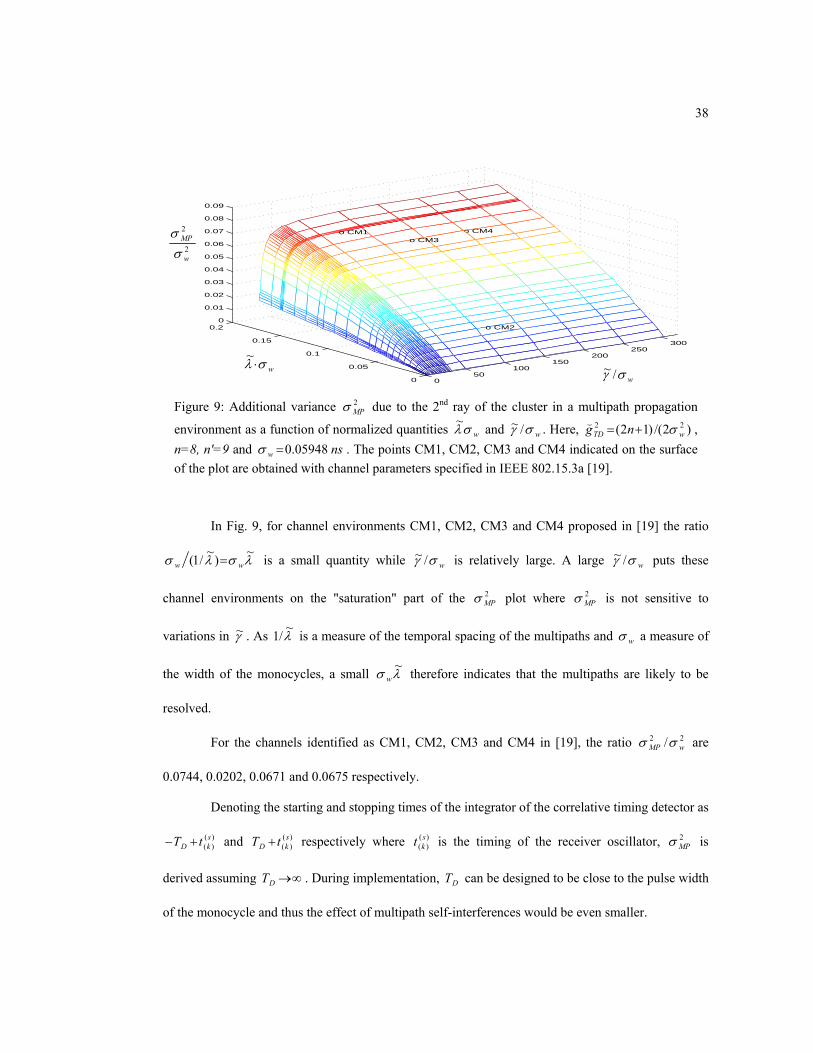
38
In Fig. 9, for channel environments CM1, CM2, CM3 and CM4 proposed in [19] the ratio
λσλσ~)~/1( ww = is a small quantity while wσγ /~ is relatively large. A large wσγ /~ puts these
channel environments on the "saturation" part of the 2MPσ plot where 2
MPσ is not sensitive to
variations in γ~ . As λ~/1 is a measure of the temporal spacing of the multipaths and wσ a measure of
the width of the monocycles, a small λσ~
w therefore indicates that the multipaths are likely to be
resolved.
For the channels identified as CM1, CM2, CM3 and CM4 in [19], the ratio 22 / wMP σσ are
0.0744, 0.0202, 0.0671 and 0.0675 respectively.
Denoting the starting and stopping times of the integrator of the correlative timing detector as
)()(
skD tT +− and )(
)(skD tT + respectively where )(
)(skt is the timing of the receiver oscillator, 2
MPσ is
derived assuming ∞→DT . During implementation, DT can be designed to be close to the pulse width
of the monocycle and thus the effect of multipath self-interferences would be even smaller.
050
100150
200250
300
0
0.05
0.1
0.15
0.20
0.01
0.02
0.03
0.04
0.05
0.06
0.07
0.08
0.09
o CM2
o CM4
o CM3o CM1
2
2
w
MP
σσ
wσλ ⋅~
wσγ /~
Figure 9: Additional variance 2MPσ due to the 2nd ray of the cluster in a multipath propagation
environment as a function of normalized quantities wσλ~ and wσγ /~ . Here, )2/()12( 22
wTD ng σ+=( , n=8, n'=9 and nsw 05948.0=σ . The points CM1, CM2, CM3 and CM4 indicated on the surface of the plot are obtained with channel parameters specified in IEEE 802.15.3a [19].

39
However it is noted in [28] that there exists a "region" in the UWB power delay profile
located beyond the arrival of the LoS signal where the power delay profile 'exhibits a single diffuse
multipath cluster caused by superposition of a large number of un-resolved paths'. There are also
'limitations imposed on resolvability imposed by the UWB antennas' [28]. If the timing detector is
tracking a NLoS component in this diffuse multipath region of the power delay profile, the analysis
performed in this section which assumes a channel with discrete impose response is no longer valid.
As a result, there will be timing error at the output of the detector due to multipath self-interferences.
In subsequent analysis, the effect of multipath self-interference on the output of the timing
detector is ignored.
2.3.4 Effect of Non-Line-of-Sight (NLoS) Signal Propagation
A NLoS signal refers to transmitted signal that arrived at the receiver after being scattered
from scattering centers distributed around the transceivers or signals that have blockages in their
signal propagation paths.
It is assumed for convenience, and lacking definitive results on UWB signal propagating
through materials in the literature, that retardation of the LoS signal passing through blockages is
negligible compared with additional propagation time via scattering8. This assertion needs further
scrutiny when more propagation data for typical environments becomes available in the open
literature. Discussion on the behavior of UWB signals passing through material can be found in [38].
In the absent of blockages, it is assumed that the first arrival is the LoS path.
In this work, the propagation delay of a signal transmitted by node m and received at node
s is modeled by
8 The distribution of scatters around transmitter has been modeled with scatter models such as ring, uniform, Gaussian, circular and elliptical [25]. However, these models are developed primarily for narrowband signals and may not be applicable for UWB signals.
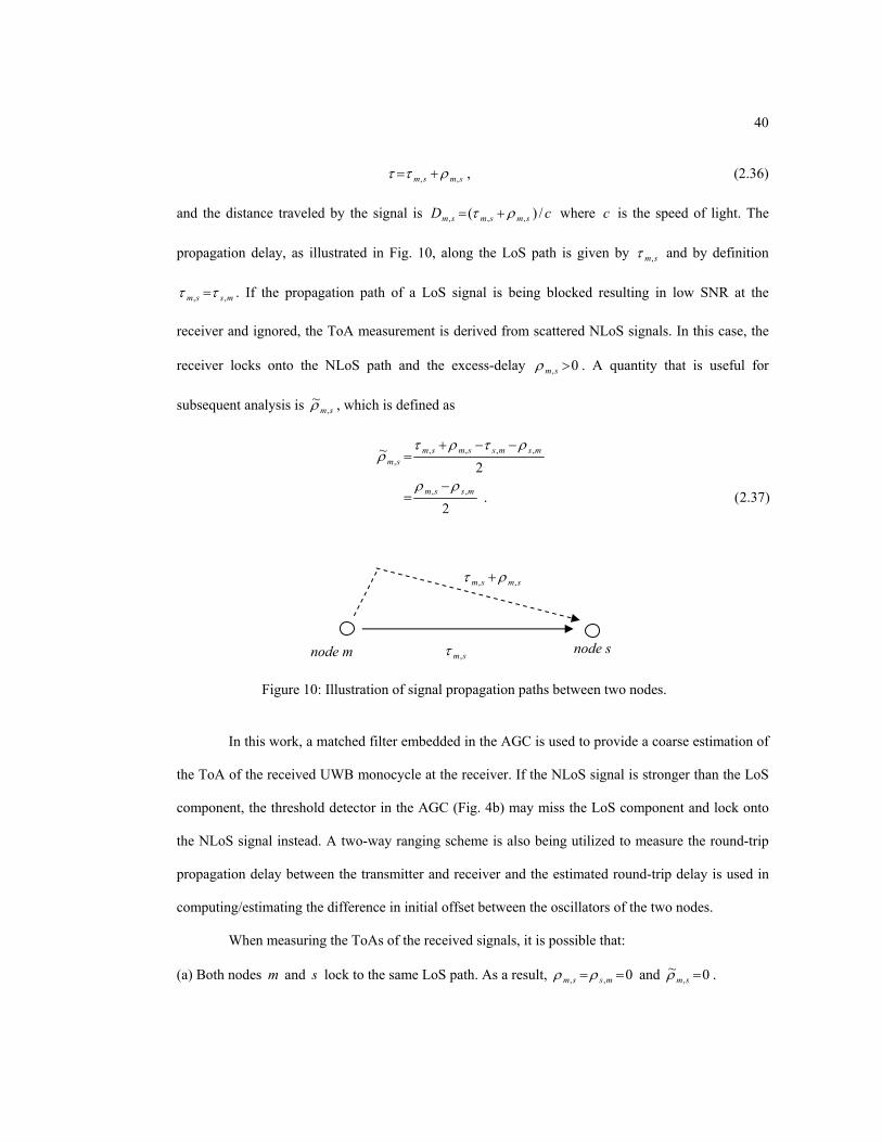
40
smsm ,, ρττ += , (2.36)
and the distance traveled by the signal is cD smsmsm /)( ,,, ρτ += where c is the speed of light. The
propagation delay, as illustrated in Fig. 10, along the LoS path is given by sm,τ and by definition
mssm ,, ττ = . If the propagation path of a LoS signal is being blocked resulting in low SNR at the
receiver and ignored, the ToA measurement is derived from scattered NLoS signals. In this case, the
receiver locks onto the NLoS path and the excess-delay 0, >smρ . A quantity that is useful for
subsequent analysis is sm,~ρ , which is defined as
)37.2(.
2
2~
,,
,,,,,
mssm
msmssmsmsm
ρρ
ρτρτρ
−=
−−+=
In this work, a matched filter embedded in the AGC is used to provide a coarse estimation of
the ToA of the received UWB monocycle at the receiver. If the NLoS signal is stronger than the LoS
component, the threshold detector in the AGC (Fig. 4b) may miss the LoS component and lock onto
the NLoS signal instead. A two-way ranging scheme is also being utilized to measure the round-trip
propagation delay between the transmitter and receiver and the estimated round-trip delay is used in
computing/estimating the difference in initial offset between the oscillators of the two nodes.
When measuring the ToAs of the received signals, it is possible that:
(a) Both nodes m and s lock to the same LoS path. As a result, 0,, == mssm ρρ and 0~, =smρ .
node m node s sm,τ
smsm ,, ρτ +
Figure 10: Illustration of signal propagation paths between two nodes.
41
(b) Both nodes m and s lock to the same path, which however is not the LoS path. As a result,
0, >smρ and 0, >msρ . From the reciprocity relationships between receiving and radiating
properties of antenna systems [59], it can be deduced that the same propagation channel is
presented to transceivers m and s . Further, if the receiver operations are identical in m and s ,
the principle of reciprocity9 implies that msmssmsm ,,,, ρτρτ +=+ , therefore mssm ,, ρρ = and
0~, =smρ .
(c) Transceivers m and s lock onto different NLoS paths. This can be due to changes in the
scattering environment. It is also possible that the receiver in individual node makes a
measurement that is different from the other node when tracking the NLoS signal (an example of a
NLoS signal is shown in Fig. 8). An algorithm (in each receiver) that attempts to avoid locking
onto different paths and find the earliest path is described in [31]. Further, due to manufacturing
tolerance, the matched filter at each node may differ.
If scatters that cause the excess delay sm,ρ "re-orientates" itself with respect to the positions
of nodes m and s before node s transmits the return-pulse, then it is likely that mssm ,, ρρ ≠ and
0|| , >smρ . This is plausible when nodes access the channel in separate time slots which are temporally
"far" apart that the scattering environment is no longer stationary. For example, consider a TDMA
scheme with 410−=fT seconds and one pulse per frame, 1000=K pulses per time slot and N nodes
in the network. If each node is to transmit during one time slot and wait for other nodes in the network
to finish their transmission in their respective time slots before transmitting again, the temporal
spacing between the first pulse of one transmission to another transmission by the same node is
110 −×=⋅⋅ NTKN f seconds.
9 Exception includes short-wave transmission over long distance [59] and HF systems on long propagation path [18].
42
Nevertheless, NLoS propagation is undesirable because NLoS signals traveled a longer
distance with larger excess delay than LoS propagation. A longer propagation delay will lead to lower
SNR at the receiver and hence higher timing jitter.
The variable sm,~ρ will be referred to as the receiver processing error in subsequent
discussion and models the asymmetry in the uplink and downlink propagation paths.
2.4 Estimating Differences in Initial Offset and Frame Repetition Rate
We assume transceivers are stationary during measurements. There are at least two different
approaches to estimate the differences in oscillator frame repetition rate and initial offset.
One possible approach is to employ a second order delay-locked loop [10] [42] at the
receiver to track the UWB pulses from the transmitter. That is, a second order tracking loop is used to
correct the difference in frame repetition rate between the transmitter and the receiver. The transmitter
will transmit a sequence of monocycles of length K to be pulled-in and tracked by the tracking loop
at the receiver, which will then estimate the difference in frame repetition rate fsm Taa ⋅− )( )(
1)(
1 and the
ToA of the UWB monocycles at the receiver.
The other possible approach is to process the output of the timing detector using a least
squares (LS) estimator without placing the detector in a tracking loop [10]. In this work, we assume
that the open loop approach is implemented to estimate the fame frequency differences.
If the timing detector is not embedded in a tracking loop, from (2.17) and wTDD AgK (/1= , the
ToA of UWB monocycles at the receiver is the output of the correlative timing detector given by
)38.2(,)/()(
)/(
)(
)()(
)()(
)()(,,
)()()(1
)(1
)()(,,
)()(
)()(
)()(,,
)()(
)()()(
TDwsk
sk
mksmsm
smf
sm
TDwsksmsm
sk
mk
skDsmsm
sk
mkTDwDk
gAnddkTaa
gAntt
nKttgAKx
(
(
(
+−+++−+−=
+++−=
+++−⋅=
φφρτ
ρτ
ρτ
where smsmsk
mkk tt ,,
)()(
)()()( ρτς ++−= .
43
Let the difference in frame repetition rate be
a)39.2(,
)(),(
)(1
)(1
),(
fsm
fsmsm
Ta
Taa
δ
γ
=
⋅−=
where )(1
)(1
),( smsm aaa −=δ and let the propagation delay from m to s plus difference in initial offset be
b)39.2(,,,
),(
,,)()(),(
smsmsm
smsmsmsm
d
dd
ρτ
ρτζ
δ ++=
++−=
where )()(),( smsm ddd −=δ . Further, let
)/()()(
)()(
)()(
)()( TDw
sk
sk
mk
m,skx gAnε (+−= φφ . (2.39c)
where 0 ),()( =sm
kxεΕ . The timing detector output given by (2.38) can be expressed as
),()(
),(),()(
smkx
smsmk kx εζγ ++⋅= . (2.40)
Denoting the variance of )(kx by ),(2 smxσ , we have
)41.2(.2),(
)()())/((
)(
),(
22
2)()(
2)()(
2)()(
2),()(
)(2
φσσ
φφ
ε
σ
+=
++=
=
=
sm
gAn
xsm
n
sk
mkTDw
sk
smkx
kx
ΕΕΕ
Ε
V
(
Equation (2.41) makes use of (2.22), that is,
2
,
2)()(
2 1))/((),(ω
σsm
TDwskn gAnsm
Θ≥= (Ε , (2.42a)
and from (2.25b),
b)42.2(.)(2
)(2
12
∫∞
∞−
≤
∆=
ωωπ
ωσ
ϕ
ϕφ
dS
D
o
A recursive implementation of the LS estimator can be found in [41]. However, the
simplicity of the LS estimator in this application leads to a simple batch processing without
computing any matrix inverses.

44
To formulate the LS estimator, consider a more general case when the output of the timing
detector is described by
),()(
),(),()(
smkx
smLSf
smk kTax εζδ ++⋅∆⋅⋅= , (2.43a)
where )(kx is obtained at the output of the detector at regular temporal spacing of fLS Tk ⋅⋅∆ for
1≥∆ LS . Equation (2.43a) can be written in vector form with K measurements, such that
+
⋅=
+
−+
−+
+
−+
−+
)()(
),()1(
),()2(
),()1(
),(
),(
)(
)1(
)2(
)1(
m,sKx
smKx
smKKx
smKKx
sm
sm
K
K
KK
KK
ST
ST
ST
ST
ST
ST
ST
ST
εxx
xx
ε
εε
ζγ
MM H , (2.43b)
where
−+⋅∆−+⋅∆=
111)2()1(L
L STSTLSSTLS KKKKKTH . (2.43c)
It can be shown that the LS estimates of ),( smγ and ),( smζ are [41]
⋅=
−+
−+
−
)(
)2(
)1(
1),(
),(
)(ˆˆ
ST
ST
ST
K
KK
KK
smLS
smLS
x
xx
MTT HHH
ζγ
. (2.43d)
From (2.43d), the LS estimators are [10]
LS
KK
KkkST
LS
KK
Kkk
smLS KK
xKK
KK
xkST
ST
ST
ST
∆⋅−⋅
−+⋅−
∆⋅−⋅
⋅=
∑∑−+
=
−+
=
)1(
)12(6
)1(
12ˆ
2
1
)(
2
1
)(),(γ , (2.43e)
,)1(
)12(6
)1(
))1(6)12)(1((2ˆ
2
1
)(
2
1
)(),(
−⋅
⋅−+⋅−
−⋅
−++−−⋅=
∑∑−+
=
−+
=
KK
xkKK
KK
xKKKKKST
ST
ST
ST
KK
KkkST
KK
KkkSTST
smLSζ (2.43f)
where 1,..., −+∈ KKKk STST if K frames are used and 0≥STK denotes the time index of the first
received pulse.

45
Substituting (2.43a) into (2.43e), we arrive at
)44.2(.)1(
)12(6)1(
12)1(
)12(6)1(
12)1(
)12(6)1(
12ˆ
1),(
)(2
1),(
)(2
1),(
2
1),(
2
1),(
2
12),(
2),(
∑∑
∑∑
∑∑
−+
=
−+
=
−+
=
−+
=
−+
=
−+
=
∆⋅−
−+−⋅
∆⋅−+
∆⋅−
−+−
∆⋅−+
⋅∆⋅∆⋅−
−+−⋅∆⋅
∆⋅−=
ST
ST
ST
ST
ST
ST
ST
ST
ST
ST
ST
ST
KK
Kk
smkx
LS
STKK
Kk
smkx
LS
KK
Kk
sm
LS
STKK
Kk
sm
LS
KK
KkLS
sm
LS
STKK
KkLS
sm
LS
smLS
KKKK
kKK
KKKK
kKK
kKK
KKk
KK
εε
ζζ
γγγ
The first two terms of (2.44) evaluate to
)
( ) a)45.2(.)1(
)12)(12(3))1(6
))12222)(1((6
12)1(
2)1)(12(612
)1(
)1()12(6
)1(12
),(32
),(
2
),(
12
2
),(
1),(
2
12),(
2
smsm
STSTSTST
STST
sm
STSTST
KK
Kk
sm
KK
Kk
smSTKK
Kk
sm
KKKK
KKKKKKKK
KKKKKKK
KKKKKKkKK
kKK
KKk
KKST
ST
ST
ST
ST
ST
γγ
γ
γ
γγ
=−−
=
⋅−+−+−−++
+−−+−
−=
−++−+−
−=
−
−+−
−
∑
∑∑
−+
=
−+
=
−+
=
The second line of (2.44) reduces to
b)45.2(.0)1(
)12(6)1(
2)1(12
)1()12(6
)1(12
),(22
),(
1),(
2
1),(
2
=
⋅⋅∆⋅−
−+−−++⋅
∆⋅−=
∆⋅−
−+−
∆⋅−∑∑
−+
=
−+
=
sm
LS
STSTST
LS
sm
KK
Kk
sm
LS
STKK
Kk
sm
LS
KKK
KKKKKK
KK
KKKK
kKK
ST
ST
ST
ST
ζζ
ζζ
Therefore, ),(),(),(ˆ smsmsmLS LSγεγγ += where the estimation error ),( sm
LSγε is indicated by the third line of
(2.44)
∑∑−+
=
−+
= ∆⋅−
−+−⋅
∆⋅−=
1),(
)(2
1),(
)(2 )1()12(6
)1(12 ST
ST
ST
STLS
KK
Kk
smkx
LS
STKK
Kk
smkx
LS
(m,s)γ KK
KKk
KKεεε . (2.45c)
From (2.43e) and (2.43f), it can be shown that the estimators are unbiased, i.e.,
0ˆ ),(),( =− smLS
sm γγΕ , (2.46a)
0ˆ ),(),( =− smLS
sm ζζΕ , (2.46b)
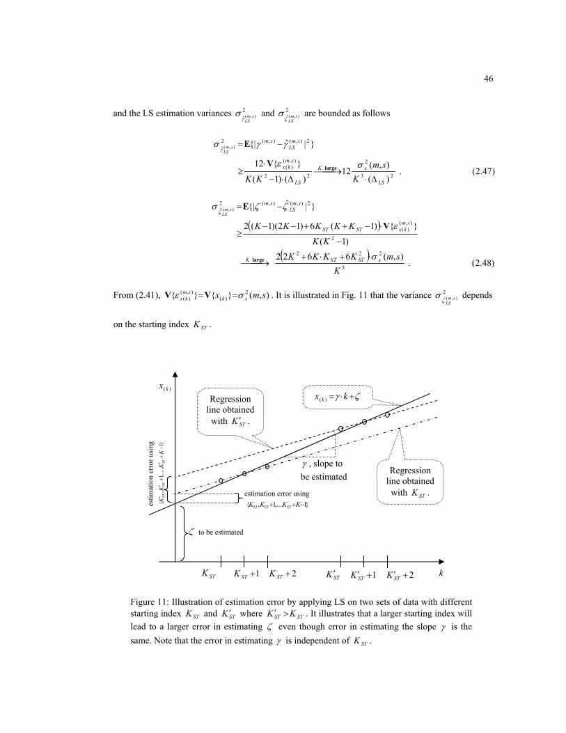
46
and the LS estimation variances 2ˆ ),( smLSγ
σ and 2ˆ ),( smLSζ
σ are bounded as follows
)47.2(.
)(),(
12)()1(
12
|ˆ|
23
2
22
),()(
2),(),(2ˆ ),(
V
Ε
large
LS
xK
LS
smkx
smLS
sm
Ksm
KK
smLS
∆⋅→
∆⋅−
⋅≥
−=
σε
γγσγ
( )
( ))48.2(.
),(6622)1(
)1(6)12)(1(2
|ˆ|
3
222
2
),()(
2),(),(2ˆ ),(
V
Ε
large
KsmKKKK
KK
KKKKK
xSTSTK
smkxSTST
smLS
smsm
LS
σ
ε
ζζσζ
⋅+⋅+→
−
⋅−++−−≥
−=
From (2.41), ),( 2)(
),()( smx xksm
kx σε ==VV . It is illustrated in Fig. 11 that the variance 2ˆ ),( smLSζ
σ depends
on the starting index STK .
Figure 11: Illustration of estimation error by applying LS on two sets of data with different starting index STK and STK ′ where STST KK >′ . It illustrates that a larger starting index will lead to a larger error in estimating ζ even though error in estimating the slope γ is the same. Note that the error in estimating γ is independent of STK .
Regression line obtained
with STK .
Regression line obtained
with STK ′ .
ζ to be estimated
)(kx
γ , slope to be estimated
ζγ +⋅= kx k )(
estimation error using 1,...,1, −++ KKKK STSTSTes
timat
ion
erro
r usi
ng
1
,...,
1,
−
+′
+′
′K
KK
KST
STST
1+STK 2+STK STK ′ 1+′STK 2+′STK k STK

47
The Cramer-Rao bound of (2.22) is the lower bound on the timing jitter of the open-loop
correlative timing detector when the disturbances are caused by AWGN in the channel. The LS
estimator is estimating the parameters ),( smγ and ),( smζ given the ToAs' measurement. Using the LS
estimator, the variance in estimating fsm Ta ),(
δ and the variance of the estimation error )ˆ( ),(),( smLS
sm ζζ −
are asymptotically inversely proportional to 3K and K respectively where K is the number of
frames used in the estimation.
According to ([41], pg.112), since
(a) the mean of the measurement error ),()(sm
kxε is zero,
(b) ),()(sm
kxε are independently identically distributed and
(c) H is deterministic,
then the LS estimator is unbiased and an efficient estimator within the class of linear estimators.
Reference [13] has derived a Cramer-Rao bound on estimating the difference in oscillator frame
repetition rate between a pair of transceivers by digitally sampling the received monocycles and
applying the least squares technique. If the sampling rate is allowed to go to infinity to generate the
continuous time bound, the bound given by [13] reduces to (2.47). Here the bound on the initial offset
is obtained as well.
In Fig. 12, the theoretical lower bounds on 2ˆLSγσ and 2
),( smLSζ
σ at different K given by (2.47)
and (2.48) for 0=STK are plotted alongside their ensemble averages (over 3000 realizations)
obtained via simulation implementing equations (2.43e) and (2.43f). In the simulation, the received
SNR is dBsm 30, =Θ , 22 /5.8 wσω = , ssm T
LS176.1 ),( =γεV , sf
sm TTaa 10)( )(1
)(1 =⋅− ,
ssm
sm Tdd 20)()(, =−+τ where sT is the sampling interval.
It should be noted that either performing LS estimation on the output of the open loop timing
detector or embedding the correlative timing detector in an error tracking loop will not be able to
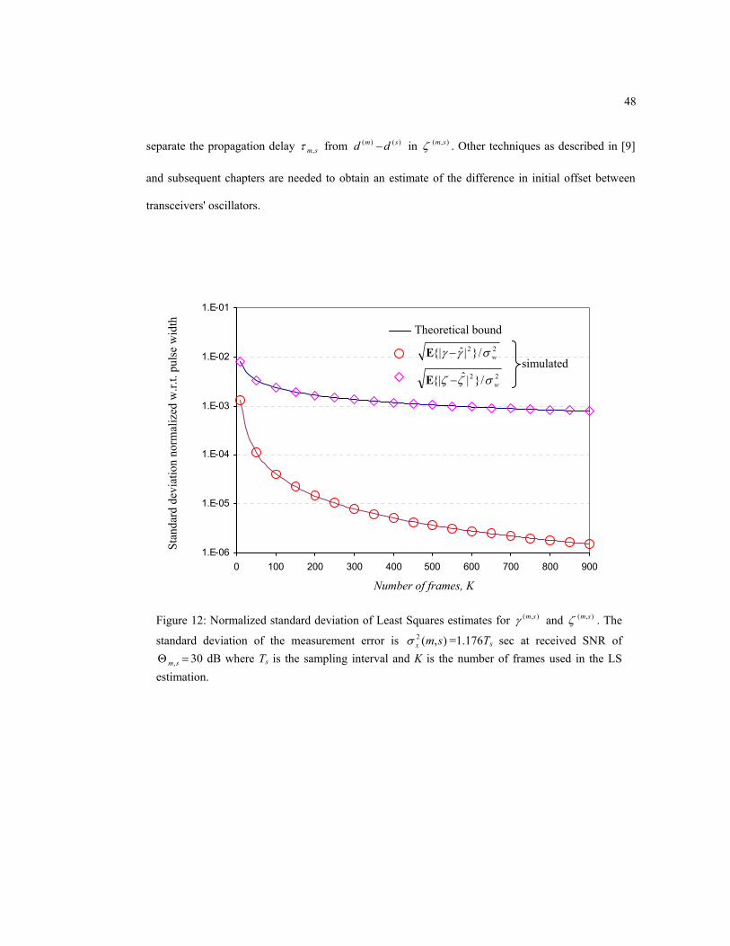
48
separate the propagation delay sm,τ from )()( sm dd − in ),( smζ . Other techniques as described in [9]
and subsequent chapters are needed to obtain an estimate of the difference in initial offset between
transceivers' oscillators.
1.E-06
1.E-05
1.E-04
1.E-03
1.E-02
1.E-01
0 100 200 300 400 500 600 700 800 900
Figure 12: Normalized standard deviation of Least Squares estimates for ),( smγ and ),( smζ . The
standard deviation of the measurement error is ),(2 smxσ =1.176Ts sec at received SNR of =Θ sm, 30 dB where Ts is the sampling interval and K is the number of frames used in the LS
estimation.
Number of frames, K
Stan
dard
dev
iatio
n no
rmal
ized
w.r.
t. pu
lse
wid
th
22 /|ˆ| wσγγ −Ε
22 /|ˆ| wσζζ −Ε
Theoretical bound
simulated
49
CHAPTER III
TIME-TRANSFER SCHEME
This Chapter describes the proposed time-transfer scheme to implement a synchronous
impulse network. The proposed time-transfer scheme consists of frame-synchronization pulses
transmitted from the master node to slave nodes to align the pulse/frame repetition rate of the slaves'
oscillator to that of the master. This is followed by two-way ranging to mitigate the unknown signal
propagation delay. The measurement system presented in Chapter 2 is utilized to measure the relative
ToA of UWB monocycles at the receiver in the presence of additive noise, oscillator phase noise, and
NLoS propagation. The estimation technique presented in Chapter 2 is also used to estimate
differences in the frame repetition rate and the initial offset between network nodes' oscillator.
Three different arrangements of the frame-synchronization, uplink and downlink frames are
presented in this Chapter. They represent three variations of the proposed time-transfer scheme.
3.1 TDMA Time-Transfer Scheme
In Fig. 13, the time-transfer scheme for two nodes (master and slave) in the network is
illustrated. The first-step of the proposed time-transfer scheme involves the master node broadcasting
frame-synchronization pulses to slave nodes to align the pulse/frame repetition rate of the slaves'
oscillator to that of the master. This is followed by two-way ranging to mitigate the unknown signal
propagation delay. The initial timing offset between the master m and slave s with timing functions
)()( tT m and )()( tT s respectively is )()( sm dd − . The signal propagation delay from m to s is
smsm ,, ρτ + where sm,ρ is the excess-delay. The difference 2/)(~,,, mssmsm ρρρ −= is used to model
receiver processing error resulting from non-symmetry of the uplink and downlink ToAs measured by
the receiver. More details on sm,~ρ are given in section 2.3.4.
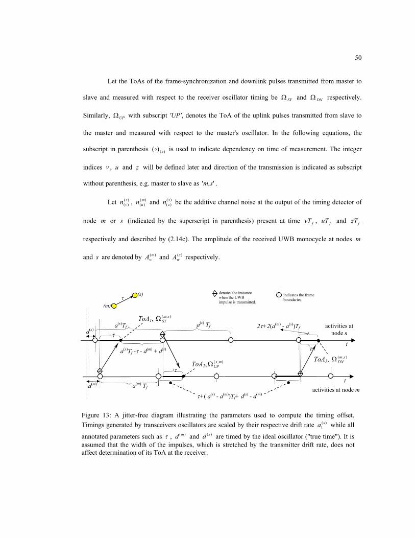
50
Let the ToAs of the frame-synchronization and downlink pulses transmitted from master to
slave and measured with respect to the receiver oscillator timing be SYΩ and DNΩ respectively.
Similarly, UPΩ with subscript 'UP', denotes the ToA of the uplink pulses transmitted from slave to
the master and measured with respect to the master's oscillator. In the following equations, the
subscript in parenthesis )()( zo is used to indicate dependency on time of measurement. The integer
indices v , u and z will be defined later and direction of the transmission is indicated as subscript
without parenthesis, e.g. master to slave as ',' sm .
Let )()(
svn , )(
)(mun and )(
)(szn be the additive channel noise at the output of the timing detector of
node m or s (indicated by the superscript in parenthesis) present at time fvT , fuT and fzT
respectively and described by (2.14c). The amplitude of the received UWB monocycle at nodes m
and s are denoted by )(mwA and )(s
wA respectively.
Figure 13: A jitter-free diagram illustrating the parameters used to compute the timing offset. Timings generated by transceivers oscillators are scaled by their respective drift rate )(
1sa while all
annotated parameters such as τ , )(md and )(sd are timed by the ideal oscillator ("true time"). It is assumed that the width of the impulses, which is stretched by the transmitter drift rate, does not affect determination of its ToA at the receiver.
d(m)
τ
a(m) Tf
τ+( a(s) - a(m))Tf+ d(s) - d(m)
tactivities at node m
a(s)Tf -τ - d(m) + d(s)
ToA1, ),( smSYΩ
ToA2, ),( msUPΩ
d(s)
τ
τa(s)Tf activities at
node s a(s) Tf 2τ+2(a(m) - a(s))Tf
t
ToA3, ),( smDNΩ
denotes the instance when the UWB impulse is transmitted.
indicates the frame boundaries.
(m)
(s) τ

51
The synchronizing scheme, illustrated in Fig. 13, works as follows. The master starts by
broadcasting frame-synchronization pulses at )()(
mvt for kKv ST += and values of k in
1,...,3,2,1,0 −sK to all other transceivers in the network. The variable 0≥STK is the starting index
of the transmitted pulses. The start of the time-transfer process is indicated by 0=STK . The slave
transceiver measures the relative ToA )(),()( ksm
vSYΩ of the thv frame-synchronization pulse with respect
to the start of its thv frame. The relative ToA, )(),()( ksm
vSYΩ is the output of the correlative timing
detector when the receiver (at node s ) is tracking the UWB monocycles transmitted from node m .
Therefore from (2.38), )(),()( )( k
smvSY xk =Ω and
)1.3(.)(
)/()(),(),(
)()()(,
)()(
)()(,
),()(
smSYST
sm(m,s)SY
TDs
wsvsm
sv
mvsm
smvSY
Kkζ
gAnttk
εγ
ρτ
++⋅+=
++−+=Ω (
where )()(),( smsm ddd −=δ , )(1
)(1
),( smsm aaa −=δ , smsm
smsm
SY d ,),(
,),( ρτζ δ ++= , f
smsm Ta ),(),(δγ = and
)/( )()()()(
),(TD
sw
svv
smSY gAn (+=µε . We have defined the random variable )(vµ as
)()(
)()()(
sv
mvv φφµ −= . (3.2)
If there are N transceivers in the network, then in its assigned time slot, e.g., time slot j ,
,...,2 Nj∈ (the index '1' is reserved for the first master node that starts the time-transfer process),
each slave transceiver will transmit rK up-link ranging pulses in contiguous frames to the master.
These pulses will arrive at the thj slot of the master node. The ToA measured with respect to the
frame boundaries of the master node is
a)3.3(.
)/()(),()(
),(),(
)()()(,
)()(
)()(,
),()(
msuUP
msmsUP
TDm
wmums
mu
sums
msuUP
u
gAnttk
εγζ
ρτ
+⋅+=
++−+=Ω (
The frame index u is measured with respect to the start of the time-transfer process. It indicates the
frame at which the uplink pulse is transmitted and is given by
STrs KkKjKu ++−+= )2( , (3.3b)
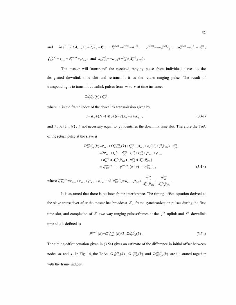
52
and 1,2,...,4,3,2,1,0 −−∈ rr KKk , )()(),( smsm ddd −=δ , fsmms Ta ),(),(
δγ −= , )(1
)(1
),( smsm aaa −=δ ,
mssm
msms
UP d ,),(
,),( ρτζ δ +−= , and )/( )()(
)()(),()( TD
mw
muu
msuUP gAn (+−= µε .
The master will 'transpond' the received ranging pulse from individual slaves to the
designated downlink time slot and re-transmit it as the return ranging pulse. The result of
transponding is to transmit downlink pulses from m to s at time instances
)()(
),()( )( m
zms
uUP tk +Ω ,
where z is the frame index of the downlink transmission given by
STrrs KkKiKNKz ++−+−+= )2()1( , (3.4a)
and i , ,..,2 Ni∈ , i not necessary equal to j , identifies the downlink time slot. Therefore the ToA
of the return pulse at the slave is
b)4.3(,)(
)/()/(
2
)/()()(
),()(
),(),(
)()()(
)()()(
,,)()(
)()(
)()(
)()(,
)()(
)()()(,
)()(
),()(,
),()(
smzDN
smsmDN
TDs
wszTD
mw
mu
mssmsu
sz
mu
mzsm
szTD
sw
szsm
mz
msuUPsm
smzDN
uz
gAngAn
tttt
tgAntkk
εγζ
ρρτ
ρτ
+−⋅+=
++
+++−−+=
−+++Ω+=Ω
((
(
where mssmsmmssm
DN ,,,,),( ρρττζ +++= and
TDm
w
mu
TDs
w
sz
uzsmzDN gA
ngA
n(( )(
)()(
)(
)()(
)()(),(
)( ++−= µµε .
It is assumed that there is no inter-frame interference. The timing-offset equation derived at
the slave transceiver after the master has broadcast sK frame-synchronization pulses during the first
time slot, and completion of K two-way ranging pulses/frames at the thj uplink and thi downlink
time slot is defined as
)(2/)()( ),()(
),()(
),( kkk smvSY
smzDN
sm Ω−Ω=ϑ . (3.5a)
The timing-offset equation given in (3.5a) gives an estimate of the difference in initial offset between
nodes m and s . In Fig. 14, the ToAs, )(),()( ksm
vSYΩ , )(),()( kms
uUPΩ and )(),()( ksm
zDNΩ are illustrated together
with the frame indices.
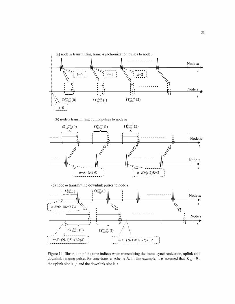
53
Figure 14: Illustration of the time indices when transmitting the frame-synchronization, uplink and downlink ranging pulses for time-transfer scheme A. In this example, it is assumed that 0=STK , the uplink slot is j and the downlink slot is i .
t
Node m
t
Node s
)0(),()(
msuUPΩ )1(),(
)(ms
uUPΩ )2(),()(
msuUPΩ
(b) node s transmitting uplink pulses to node m
u=K+(j-2)K u=K+(j-2)K+2
t
Node m
t
Node s
)0(),()(
smzDNΩ )1(),(
)(sm
zDNΩ
(c) node m transmitting downlink pulses to node s
z=K+(N-1)K+(i-2)K z=K+(N-1)K+(i-2)K+2
t
t
Node m
Node s
)0(),()(
smvSYΩ )1(),(
)(smvSYΩ )2(),(
)(smvSYΩ
(a) node m transmitting frame-synchronization pulses to node s
t=0
k=0 k=1 k=2
)0(),()(
msuUPΩ )1(),(
)(ms
uUPΩ
z=K+(N-1)K+(i-2)K

54
For simplicity, in subsequent analysis, we consider the case in which rs KKK == and ji= .
If there are K measurements of )(),( ksmϑ , 1,...,2,1,0 −∈ Kk , then collecting these K
measurements, (3.5a) can be expressed in vector form as
ΩΩΩ
−Ω
−
ΩΩΩ
−Ω
=
−
)0()1()2(
)1(
)0()1()2(
)1(
21
)0()1()2(
)1(
),()(
),()(
),()(
),()(
),()(
),()(
),()(
),()(
),(
),(
),(
),(
smvSY
smvSY
smvSY
smvSY
smzDN
smzDN
smzDN
smzDN
sm
sm
sm
sm KKKMMM
ϑϑϑ
ϑ
. (3.5b)
That is,
),()(
),()(
),(
21 sm
vSYsm
zDNsm Ω−Ω⋅=
rrrϑ , (3.5c)
where
ΩΩΩ
−Ω
=Ω
)0()1()2(
)1(
),()(
),()(
),()(
),()(
),()(
smzDN
smzDN
smzDN
smzDN
smzDN
KM
r,
ΩΩΩ
−Ω
=Ω
)0()1()2(
)1(
),()(
),()(
),()(
),()(
),(
smvSY
smvSY
smvSY
smvSY
smSY
KM
r and
−
=
)0()1()2(
)1(
),(
),(
),(
),(
),(
sm
sm
sm
sm
sm
K
ϑϑϑ
ϑ
ϑM
r.
Substituting (3.1) and (3.4b) into (3.5a) gives
a)6.3(,22
)2()(2
)()(
2
2
21
2)(
),(,,)()()(
1)(
1
),(,,)()()(1
)(1
)(1
)(1
)(1
)(1
,,
)(
)()(
)(
)()(
)(
)()(
)()(
)()(
)()(
)()(
)()(
)()(),(
smsmmsmsfsm
smsmmsmsfST
sfST
m
fs
fm
fm
fs
smms
TDs
w
sv
TDs
w
sz
TDm
w
mu
sv
mv
su
sz
mu
mzsm
ddTvuzaa
ddTKkaTKka
zTazTauTauTa
gA
n
gA
n
gA
n
tttttt
k
ϑ
ϑ
ερρ
ερρ
ρρ
ϑ
+−
+−+⋅−−⋅−
=
+−
+−+⋅+⋅+⋅+⋅−
−+−=
−+
−
++
+−+−−
=
(((
55
where ),( smϑε is the random fluctuation with zero mean given by
b)6.3(.2
)/()/(2
2)/()/(
2)()(
)()()(
)()(
)()(
)()()(
)()()(
)()()(
)(
)()()(
)()(
)(
)()(
)()(
)()(
)()(),(
TDs
wszTD
mw
mu
TDs
w
sv
vuz
TDs
wszTD
mw
mu
TDs
w
svs
vmv
sz
mz
mu
susm
gAngAn
gA
n
gAngAn
gA
n
((
(
((
(
++−−
−=
++−+−
−+−=
µµµ
φφφφφφ
εϑ
It is assumed that the oscillator phase noise, )()(
mkφ and )(
)(skφ , ,, zuvk∈ are i.i.d., therefore
2)(
2)(
2)( vuz µµµ ΕΕΕ == . (3.7a)
From (2.25a) and (2.25b),
22)()(
)()(
2)( 2)( φσφφµ =−= s
vmvv ΕΕ . (3.7b)
The noise variances are
),(2)(
)()(
)(
)()( sm
A
n
A
nn
TDs
w
sz
TDs
w
sv σ
µµ=
=
ΕΕ , (3.8a)
),(2)(
)()( ms
An
nTD
mw
mu σµ
=
Ε . (3.8b)
Therefore the variance of ),( smϑε is
)9.3(,
4),(),(5
),(41),(
45)2(
23
22
222),(
V
mssm
mssm
xx
nnsm
σσ
σσσε φϑ
+⋅=
⋅+⋅+⋅=
where ),(2),( 222 smsm nx σσσ φ += . In (3.6a), )(),( ksmϑ is a function of the initial offset and is
independent of the propagation delay between nodes m and s if 0., =− mssm ρρ . The short-term
variations in (3.6b) are assumed to have zero means.
Note that for the time-transfer scheme illustrated in Fig. 14, the difference in the downlink
and uplink frame index is
)10.3(.)1(
)1( KN
KjiNuz r
−=−+−=−
56
From (3.6a), it is observed that if )(1
)(1
sm aa = , then |)(| ),( ksmϑ is not a function of time index k .
Since 2/)(~,,, mssmsm ρρρ −= , )()(),( smsm ddd −=δ , )(
1)(
1),( smsm aaa −=δ and for ji= , let
)11.3(.2
2)1(2
2)1(2
2)(
kKN
kKjiN
kuzk
r
−−=
−−+−=
−−=θ
The quantity )(kθ is a function of the transmission index of the frame-synchronization, uplink and
downlink pulses and is specific to the time-transfer scheme shown in Fig. 14. The function )(kθ will
be called the characteristics function of the time-transfer scheme in subsequent analysis. Replacing
2/)2( kuz −− in (3.6a) with )(kθ , the initial-offset equation becomes
)12.3(.))((~
)(2
)()(
),(),(,
),(
),(),(
)(),(
fsm
STsm
smsm
smSY
smzDNsm
TaKkd
kk
k
δϑδ θερ
ϑ
⋅−++−−=
Ω−Ω
=
3.2 Bounds on Number of Network Nodes
As mentioned earlier, the proposed time-transfer scheme assumed that monocycles arrived at
the receiver at its designated frame within specific time slots. In the absence of noise and interference,
the differences in the frame repetition rate fsm
fsm TaaTa ⋅−= )( )(
1)(
1),(
δ and initial offset
)( )()(),( smsm ddd −=δ between master and slaves determine the number of nodes N we can place in
the network such that UWB impulses would arrive at the designated time slots and the TDMA scheme
is not violated. Further, to avoid inter-frame interference, let τ ′ includes the delay spread of the
channel10.
10 In IEEE 802.15.3a UWB channel model [19], the channel models CM1, CM2, CM3 and CM4 specifies root-mean-squares delay spread of 5, 8, 14 and 26 nanoseconds respectively.
57
Although nodes access the channel by time division multiplexing, nodes in the network have
different initial offsets, frame repetition rates and transmitted pulses travelled different distances
before arriving at, for example, the master node. As a result, as illustrated in Fig. 15, it is not always
possible that there is only one received monocycle (corresponds to each transmitter) per frame, being
received at the master node. In order for the master node to perform transponding and transfer its
timing to the slave nodes, the master node must be able to associate the received monocycles with the
transmitter. And hence there are bounds on the number of network nodes given the maximum
differences in oscillator parameters among pair of network nodes.
The first bound on N can be deduced from the requirement that 1ToA , )(),()( ksm
vSYΩ
(illustrated in Figs. 13 and 14) needs to be within the designated receiving time slot of the slave
transceiver, and for the last transmitted pulse in the time slot, fs
ssmvSY TaK )(
1),()( )1(0 <−Ω< . With
0=STK , this leads to the inequalities
)()(),( )1( msfs
sm ddTKa −>′+⋅−⋅ τδ , (3.13a)
fs
fssmms TaTKadd )(
1),()()( )1( −′+⋅−⋅>− τδ . (3.13b)
Applying a similar restriction on 2ToA , )(),()( kms
uUPΩ for 0),( >frsm TKaδ and analyzing the typical case
when Nj = , 1−= rKk in (3.3a), produces the inequalities
frsm
rsfsm
fmsm
TKa
KKTaTadN
),(
),()(1
),( )1(
δ
δδ τ −−−−′+−> , (3.14a)
frsm
rsfsmsm
TKa
KKTadN
),(
),(),( )1(
δ
δδ τ −−⋅−′+−< . (3.14b)
For 0),( >frsm TKaδ , the bound on 3ToA , )(),(
)( ksmzDNΩ and for 1−= rKk is f
sr
smzDN TaK )(
1),(
)( )1(0 <−Ω< .
This leads to
12),(
++−−
′> ji
TKaN
frsm
δ
τ , (3.15a)

58
12
),(
)(1 ++−
′−< ji
TKa
TaN
frsm
fs
δ
τ. (3.15b)
The corresponding inequalities on N if 0),( <frsm TKaδ can be derived similarly. The upper bound on
N for master-slave time-transfer is obtained by combining the inequalities (3.13), (3.14) and (3.15)
and their dual when 0),( <fsm KTaδ .
To obtain numerical values on N , the communicating range of the UWB transceiver is
assumed to be between 1 and 10 m, therefore the LoS propagation delay between two nodes m and
s , denoted by sm,τ , is in the order of 3x 810− sec. In Fig. 16, we plotted the upperbound on N with
∈′τ 10-8, 2x10⁻⁸, 3x10⁻⁸ sec, ignoring NLoS measurement error, considering ∈fT 10-3, 10-4, 10-6
sec and 0>N , )()( sm dd = , 1)(1 =ma and η±= )(
1)(
1ms aa where η is a small number that represents the
largest difference in drift between pair of oscillators in the network. We have arbitrarily let
K = sK = rK =512 and ji = in Fig. 16. It illustrates that at η =10-9, τ ′=3×10⁻⁸ and fT =10-3, 120<N .
For a fixed number of frames, a longer fT implies that for the same drift difference ||η , the
oscillator in each node would have drifted further apart than when fT is small for the same elapsed
"true" time (the time measured by the standard source). Thus a UWB monocycle transmitted in the
last frame of the ranging time slot and propagates to the receiver with a finite propagation delay
would not arrive within its designated time slot if ||η is not sufficiently small. Thus fewer nodes can
be supported when frame times fT are longer.
For a given fT and τ ′>>fT , if the propagation delay τ ′ is short, because of difference in
frame repetition rate, a transmitted pulse would arrive at the receiver before its designated time slot as
the transmitter and receiver oscillators drift further apart.
The situations mentioned in the previous two paragraphs (illustrated in Fig. 17) will lead to
multiple or no received monocycle at the receiver.
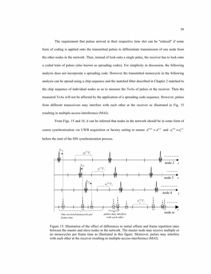
59
The requirement that pulses arrived at their respective time slot can be "relaxed" if some
form of coding is applied onto the transmitted pulses to differentiate transmission of one node from
the other nodes in the network. Then, instead of lock-onto a single pulse, the receiver has to lock-onto
a coded train of pulses (also known as spreading codes). For simplicity in discussion, the following
analysis does not incorporate a spreading code. However the transmitted monocycle in the following
analysis can be spread using a chip sequence and the matched filter described in Chapter 2 matched to
the chip sequence of individual nodes so as to measure the ToAs of pulses at the receiver. Then the
measured ToAs will not be affected by the application of a spreading code sequence. However, pulses
from different transceivers may interfere with each other at the receiver as illustrated in Fig. 15
resulting in multiple-access-interference (MAI).
From Figs. 15 and 16, it can be inferred that nodes in the network should be in some form of
coarse synchronization via UWB acquisition or factory setting to ensure )()( sm dd ≈ and )(1
)(1
sm aa ≈
before the start of the SIN synchronization process.
Figure 15: Illustration of the effect of differences in initial offsets and frame repetition rates between the master and slave nodes in the network. The master node may receive multiple or no monocycles per frame time as illustrated in this figure. Moreover, pulses may interfere with each other at the receiver resulting in multiple-access-interference (MAI).
τ4,m
τ2,m
node 4
t
t node 3
node 2 τ3,m
t
node m t
f
m Ta )(1
fTa )2(
1
fTa )3(
1
fTa )4(
1
One received monocycle per frame time
pulses may interfere with each other

60
ττ
fs Ta )(
1
fm Ta )(
1
No pulses landed in this receiver time slot
t
t node s
node m
τ
(b) Difference in frame rate is large relative to propagation delay τ
τ τ ττ
fs Ta )(
1 Two pulses landed in the same receiver time slot
t node s
fm Ta )(
1 t node m
(a) Difference in frame rate is large relative to time needed for synchronization
Figure 17: Illustration of cases when there is no or multiple received monocycles per frame time at the receiver.
Figure 16: Upper bound on the number of nodes in the network N when the difference in oscillator drift η is allows to vary assuming there is no jitter or measurement errors and K=512. The y-axis is in log scale.
1.E+00
1.E+01
1.E+02
1.E+03
1.E+04
1.E+05
1.E+06
1.E+07
0.0E+00 5.0E-10 1.0E-09 1.5E-09 2.0E-09 2.5E-09 3.0E-09
Tf=10-4
Tf=10-3
τ' =1x10⁻⁸
τ' =2x10⁻⁸
τ' =3x10⁻⁸ N
|η|
Tf=10-6 N
umbe
r of n
odes

61
3.3 Oscillator Timing Adjustment
Timing is said to have transferred from one node to another if both oscillators are ticking at
the same time after synchronization. This entails that both nodes, after time-transfer, have the same
initial offset )(md with respect to the true time t and the same drift )(1
ma . If nothing is done to effect
the time-transfer, the timing of both nodes will drift further apart as " t " progresses. For example, for
a length of time equivalent to the duration needed to perform time transfer using the synchronization
scheme proposed in section 3.1, the timing difference between a pair of nodes m and s would have
been (ignoring all the zero mean random variables/disturbances)
),(),()())12((
)())12(( )1(2 sm
fsms
KNm
KN dKNTatt δδ +−⋅=− −− . (3.16)
Thus )()(),( smsm ddd −=δ and )(1
)(1
),( smsm aaa −=δ have to be estimated from the ToA measurements
10
),()( )( −
=Ω Kk
smvSY k , 1
0),()( )( −
=Ω Kk
msuUP k and 1
0),(
)( )( −=Ω K
ksm
zDN k to correct for the accumulated timing error. There
are various ways to derive an estimate of ),( smdδ and ),( smaδ from the ToA measurements depending on
the design criteria.
The bounds, shown in Fig. 16, on the number of network nodes that can be synchronized
with the proposed time transfer scheme are derived without taking into considerations the effects of
the oscillator phase noise and additive noise in the channel. No processing is performed on the
measured ToAs to estimate and correct for the initial offset and frame repetition rate differences until
possibly at the end of the two-way ranging. These bounds indicate that in order to maximize the
number of nodes in the network, the difference in frame repetition rate must be as small as possible.
In this work, we set off to design a synchronous impulse network that is capable of
synchronizing as many nodes as possible for applications such as implementing a time-synchronous
sensor network. Thus the first task of the proposed synchronization scheme is to synchronize the
frame repetition rate of all nodes in the network.
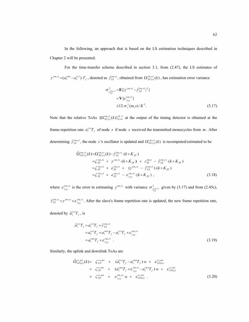
62
In the following, an approach that is based on the LS estimation techniques described in
Chapter 2 will be presented.
For the time-transfer scheme described in section 3.1, from (2.47), the LS estimates of
fsmsm Taa ⋅−= )( )(
1)(
1),(γ , denoted as ),(ˆ sm
LSγ , obtained from )(),()( ksm
vSYΩ , has estimation error variance
)17.3(./),(12
|ˆ|
32
),(
2),(),(2ˆ ),(
V
Ε
Ksmx
sm
smLS
sm
LS
smLS
σ
ε
γγσ
γ
γ
⋅≥
=
−=
Note that the relative ToAs 10
),()( )( −
=Ω Kk
smvSY k at the output of the timing detector is obtained at the
frame-repetition rate fs Ta )(
1 of node s if node s received the transmitted monocycles from m . After
determining ),(ˆ smLSγ , the node s 's oscillator is updated and )(),(
)( ksmvSYΩ is recomputed/estimated to be
)18.3(,)(
)()ˆ(
)(ˆ(
)(ˆ)()(ˆ
),(),(),(
),(),(),(),(
),(),(),(
),(),()(
),()(
)
STsmsm
SYsm
SY
STsm
LSsmsm
SYsm
SY
STsm
LS(m,s)SYST
smsmSY
STsm
LSsmvSY
smvSY
Kk
Kk
Kk εKk
Kkkk
LS+⋅−+=
+⋅−++=
+⋅−++⋅+=
+⋅−Ω=Ω
γεεζ
γγεζ
γγζ
γ
where ),( smLSγε is the error in estimating ),( smγ with variance 2
ˆ ),( smLSγ
σ given by (3.17) and from (2.45c),
),(),(),(ˆ smsmsmLS LSγεγγ += . After the slave's frame repetition rate is updated, the new frame repetition rate,
denoted by fs Ta )(
1ˆ , is
)19.3(.
ˆˆ
),()(1
),()(1
)(1
)(1
),()(1
)(1
smf
m
smf
sf
mf
s
smLSf
sf
s
LS
LS
Ta
TaTaTa
TaTa
γ
γ
ε
ε
γ
+=
+−+=
+=
Similarly, the uplink and downlink ToAs are
)20.3(.
)(
)ˆ()(ˆ
),()(
),(),(
),()(
)(1
),()(1
),(
),()(
)(1
)(1
),(),()(
msuUP
smmsUP
msuUPf
msmf
mmsUP
msuUPf
mf
smsUP
msuUP
u ζ
u TaTa ζ
u TaTa k
LS
LS
εε
εε
εζ
γ
γ
+⋅+=
+⋅−++=
+⋅−+=Ω
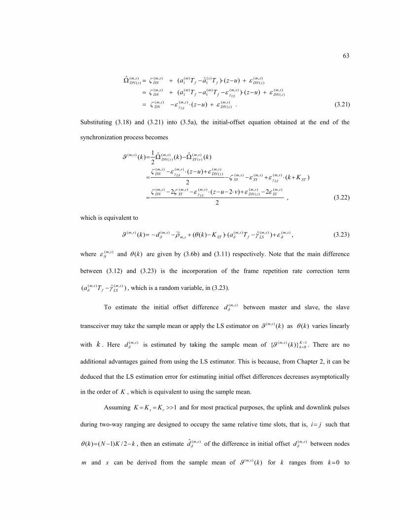
63
)21.3(.)(
)()(
)()ˆ(ˆ
),()(
),(),(
),()(
),()(1
)(1
),(
),()(
)(1
)(1
),(),()(
smzDN
smsmDN
smzDN
smf
mf
msmDN
smzDNf
sf
msmDN
smzDN
uz ζ
uzTaTa ζ
uzTaTa ζ
LS
LS
εε
εε
ε
γ
γ
+−⋅−=
+−⋅−−+=
+−⋅−+=Ω
Substituting (3.18) and (3.21) into (3.5a), the initial-offset equation obtained at the end of the
synchronization process becomes
)22.3(,2
2)2(2
)(2
)(
)(ˆ)(ˆ21)(
),(),()(
),(),(),(
),(),(),(),()(
),(),(
),()(
),()(
),(
sm
SYsmzDN
smsmSY
smDN
STsmsm
SYsm
SY
smzDN
smsmDN
smvSY
smzDN
sm
vuzζ
Kkuzζ
kkk
LS
LS
LS
εεεζ
εεζεε
ϑ
γ
γγ
−+⋅−−⋅−−=
+⋅+−−+−⋅−
=
Ω−Ω=
which is equivalent to
),(),(),(,
),(),( )ˆ())((~)( smsmLSf
smSTsm
smsm TaKkdk ϑδδ εγθρϑ +−⋅−+−−= , (3.23)
where ),( smϑε and )(kθ are given by (3.6b) and (3.11) respectively. Note that the main difference
between (3.12) and (3.23) is the incorporation of the frame repetition rate correction term
)ˆ( ),(),( smLSf
sm Ta γδ − , which is a random variable, in (3.23).
To estimate the initial offset difference ),( smdδ between master and slave, the slave
transceiver may take the sample mean or apply the LS estimator on )(),( ksmϑ as )(kθ varies linearly
with k . Here ),( smdδ is estimated by taking the sample mean of 10
),( )( −=
Kk
sm kϑ . There are no
additional advantages gained from using the LS estimator. This is because, from Chapter 2, it can be
deduced that the LS estimation error for estimating initial offset differences decreases asymptotically
in the order of K , which is equivalent to using the sample mean.
Assuming 1>>== rs KKK and for most practical purposes, the uplink and downlink pulses
during two-way ranging are designed to occupy the same relative time slots, that is, ji= such that
kKNk −−= 2/)1()(θ , then an estimate ),(ˆ smdδ of the difference in initial offset ),( smdδ between nodes
m and s can be derived from the sample mean of )(),( ksmϑ for k ranges from 0=k to
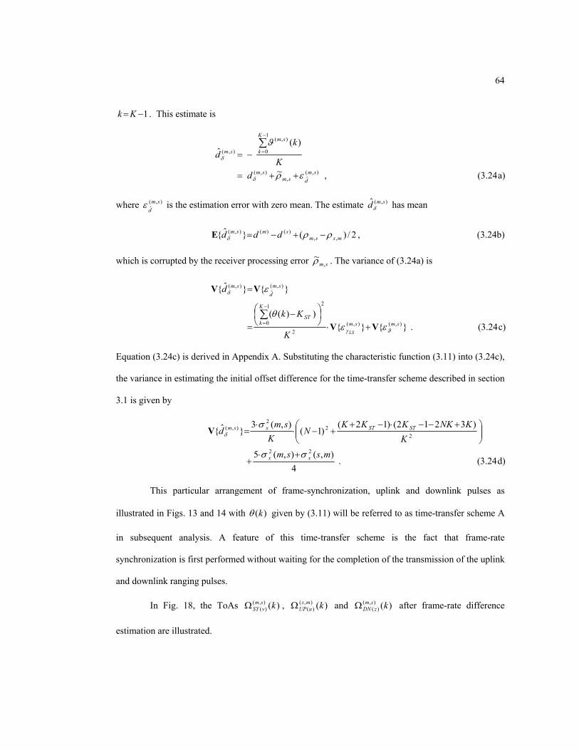
64
1−=Kk . This estimate is
a)24.3(,~
)(ˆ
),(ˆ,
),(
1
0
),(
),(
smdsm
sm
K
k
sm
sm
dK
kd
ερ
ϑ
δ
δ
++=
−=∑−
=
where ),(ˆ
smd
ε is the estimation error with zero mean. The estimate ),(ˆ smdδ has mean
2/)(ˆ ,,)()(),(
mssmsmsm ddd ρρδ −+−=Ε , (3.24b)
which is corrupted by the receiver processing error sm,~ρ . The variance of (3.24a) is
c)24.3(.))((
ˆ
),(),(2
21
0
),(ˆ
),(
VV
VV
smsm
K
kST
smd
sm
LSK
Kk
d
ϑγ
δ
εεθ
ε
+⋅
−
=
=
∑−
=
Equation (3.24c) is derived in Appendix A. Substituting the characteristic function (3.11) into (3.24c),
the variance in estimating the initial offset difference for the time-transfer scheme described in section
3.1 is given by
d)24.3(.4
),(),(5
)3212()12()1(
),(3ˆ
22
22
2),(
V
mssmK
KNKKKKN
Ksm
d
xx
STSTxsm
σσ
σδ
+⋅+
+−−⋅−++−⋅
⋅=
This particular arrangement of frame-synchronization, uplink and downlink pulses as
illustrated in Figs. 13 and 14 with )(kθ given by (3.11) will be referred to as time-transfer scheme A
in subsequent analysis. A feature of this time-transfer scheme is the fact that frame-rate
synchronization is first performed without waiting for the completion of the transmission of the uplink
and downlink ranging pulses.
In Fig. 18, the ToAs )(),()( ksm
vSYΩ , )(),()( kms
uUPΩ and )(),()( ksm
zDNΩ after frame-rate difference
estimation are illustrated.

65
k
),( msUPζ
0 1 2 3 4 K-2 K-1
)(),()( ksm
zDNΩ
k ),( sm
DNζ
0 1 2 3 4 K-2 K-1
)(),( ksmϑ
k
)(2/)()( ),()(
),()(
),( kkk smvSY
smzDN
sm Ω−Ω=ϑ
smsmd ,),( ~ρδ −−
0 1 2 3 4 K-2 K-1
Figure 18: Illustration of the ToAs measured during the frame-synchronization, uplink and downlink time slots. In this example rs KKK == .
)(),()( ksm
vSYΩ
k 0 1 2 3 4 K-2 K-1
regression line before frame rate synchronization
regression line after frame rate synchronization
)(),()( kms
uUPΩ
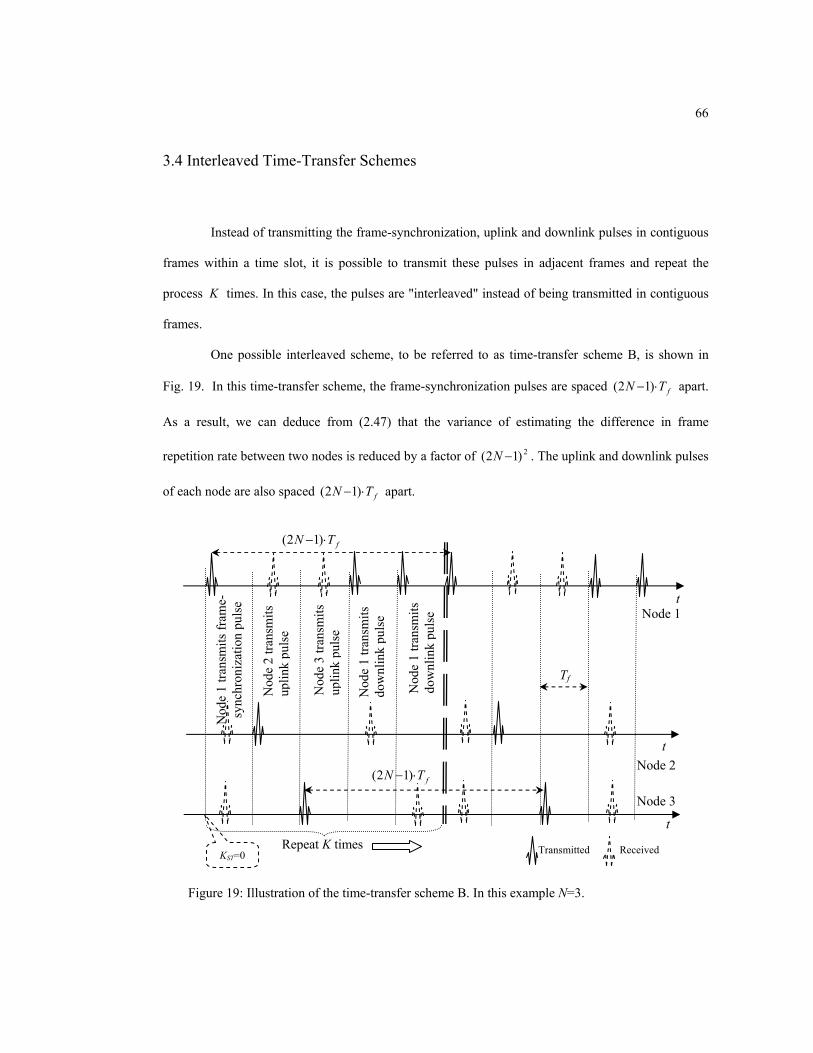
66
3.4 Interleaved Time-Transfer Schemes
Instead of transmitting the frame-synchronization, uplink and downlink pulses in contiguous
frames within a time slot, it is possible to transmit these pulses in adjacent frames and repeat the
process K times. In this case, the pulses are "interleaved" instead of being transmitted in contiguous
frames.
One possible interleaved scheme, to be referred to as time-transfer scheme B, is shown in
Fig. 19. In this time-transfer scheme, the frame-synchronization pulses are spaced fTN ⋅− )12( apart.
As a result, we can deduce from (2.47) that the variance of estimating the difference in frame
repetition rate between two nodes is reduced by a factor of 2)12( −N . The uplink and downlink pulses
of each node are also spaced fTN ⋅− )12( apart.
Figure 19: Illustration of the time-transfer scheme B. In this example N=3.
t
t
Node 1
Node 2
KST=0
Nod
e 1
trans
mits
fram
e-s y
nchr
oniz
atio
n pu
lse
Nod
e 2
trans
mits
u p
link
puls
e
Nod
e 3
trans
mits
u p
link
puls
e
Nod
e 1
trans
mits
do
wnl
ink
puls
e
Nod
e 1
trans
mits
do
wnl
ink
puls
e
t
Node 3
fTN ⋅− )12(
Tf
Transmitted Received Repeat K times
fTN ⋅− )12(
67
For this time-transfer scheme to be feasible, it is assumed that the receiver can discern the
pulses transmitted from different nodes in the network and there is no or minimum collision of pulses,
i.e., minimum MAI. In order to update the timing of the nodes correctly, the receiver must at least be
able to associate the received pulses with the transmitter that it is engaged in time-transfer. A more
detail discussion on separating the pulses at the receiver is given in section 3.2.
In this scheme, the ToAs measured with respect to the receiver's oscillator frame boundaries
are
.))12((
)(),(),(
),(),(),()(
smSYSTf
sm(m,s)SY
smSYf
sm(m,s)SY
smvSY
KkNTaζ
vTaζk
ε
ε
δ
δ
++⋅−⋅⋅+=
+⋅⋅+=Ω (3.25)
where STKkNv +⋅−= )12( and 1,...,0 −∈ rKk . The measured uplink ToAs are given by
),()(
),(),(),()( )( ms
uUPfsmms
UPms
uUP uTak εζ δ +⋅⋅+=Ω , (3.26a)
where the uplink frame index is
STKNkju +−⋅+−+= )12()2(1 , (3.26b)
and ,...,5,4,3,2 Nj∈ indicates the slot occupy by individual node. The measured downlink ToAs are
,)()( ),()(
),(),(),()(
smzDNf
smsmDN
smzDN uzTak εζ δ +−⋅⋅+=Ω (3.27a)
where the downlink pulses are transmitted at frames
STKNkiNz +−⋅+−+= )12()2( , (3.27b)
with i ( i not necessary equal to j ), ,..,2 Ni∈ , identifies the downlink time slot. In subsequent
analysis, the case ji= is analyzed.
Since 1−=− Nuz , equation (3.27a) reduces to
,)1()( ),()(
),(),(),()(
smzDNf
smsmDN
smzDN NTak εζ δ +−⋅⋅+=Ω (3.27c)
and the timing-offset equation derived at node s is
a)28.3(.
2))((
2
)(2/)()(
),(),()(),(),(
),(
),(),()(
),(
smSY
smzDN
STfsmsm
SY
smDN
smSY
smzDN
sm
KkTa
kkk
εε
θζζ
ϑ
δ −+−⋅⋅+−=
Ω−Ω=
68
The characteristic function of this time-transfer scheme is
kNNk ⋅−−−
= )12(2
1)(θ . (3.28b)
Using the LS estimator described in section 2.4, the variance in estimating ),( smγ is given by equation
(2.47), however now the frame-repetition pulses are spaced fTN ⋅− )12( apart rather than fT
compared to time-transfer scheme A, therefore
23
2),(2
ˆ )12(),(12
),(−⋅
⋅≥=
NKsmxsm
LSsmLS
σεσ γγ
V . (3.29)
For the time-transfer scheme depicted in Fig. 19, substituting (3.28b) into (3.28a), the variance in
estimating the initial offset difference between node m and s is
( )
)30.3(.4
),(),(5
2)1()12()1(41
))((
ˆ
22
),(22
),(),(2
21
0),(
V
VVV
Kmssm
KKNN
K
Kkd
xx
smST
smsm
K
kST
sm
LS
LS
σσ
ε
εεθ
γ
ϑγδ
+⋅+
⋅⋅−−⋅−−−⋅=
+⋅
−
=∑−
=
where ),( smLSγεV is given by (3.29).
An alternative interleaved scheme, to be referred to as time-transfer scheme C, is illustrated
in Fig. 20. In this time-transfer scheme, the frame-synchronization pulses are spaced fTN ⋅− )12(
apart while the uplink and downlink pulses of each node are spaced fT in time.
In both time-transfer schemes B and C, unlike time-transfer scheme A, the synchronization
of the frame repetition rate between m and s is performed after the transmission of the uplink and
downlink ranging pulses. That is, the slave node s collects all the necessary relative ToA
measurements and performs post-processing on the measurements to estimate the initial offset and
frame repetition rate differences.
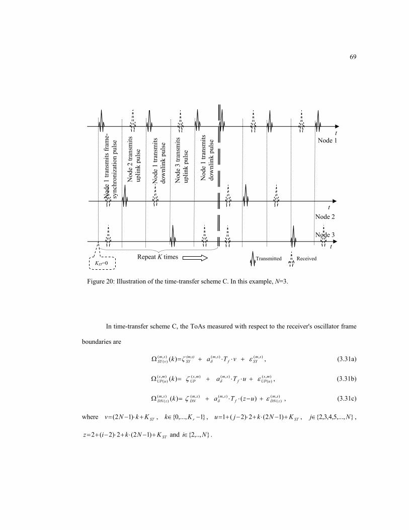
69
In time-transfer scheme C, the ToAs measured with respect to the receiver's oscillator frame
boundaries are
),(),(),()( )( sm
SYfsm(m,s)
SYsmvSY vTaζk εδ +⋅⋅+=Ω , (3.31a)
),()(
),(),(),()( )( ms
uUPfsmms
UPms
uUP uTak εζ δ +⋅⋅+=Ω , (3.31b)
,)()( ),()(
),(),(),()(
smzDNf
smsmDN
smzDN uzTak εζ δ +−⋅⋅+=Ω (3.31c)
where STKkNv +⋅−= )12( , 1,...,0 −∈ rKk , STKNkju +−⋅+⋅−+= )12(2)2(1 , ,...,5,4,3,2 Nj∈ ,
STKNkiz +−⋅+⋅−+= )12(2)2(2 and ,..,2 Ni∈ .
Figure 20: Illustration of the time-transfer scheme C. In this example, N=3.
t
t
Node 1
Node 2
KST=0
Nod
e 1
trans
mits
fram
e-s y
nchr
oniz
atio
n pu
lse
Nod
e 2
trans
mits
u p
link
puls
e
Nod
e 3
trans
mits
u p
link
puls
e
Nod
e 1
trans
mits
do
wnl
ink
puls
e
Nod
e 1
trans
mits
do
wnl
ink
puls
e
t
Node 3
Repeat K times Transmitted Received

70
Since 1=−uz , the characteristic function of the time-transfer scheme is
kNk ⋅−−= )12(21)(θ , (3.32a)
and the timing-offset equation derived at node s is
( )
b)32.3(.2
)12(21
2
2)(
2
)(2/)()(
),(),()(),(),(
),(
),(),()(),(),(
),(
),()(
),()(
),(
smSY
smzDN
STfsmsm
SY
smDN
smSY
smzDN
STfsmsm
SY
smDN
smvSY
smzDN
sm
KkNTa
KkTa
kkk
εε
ζζ
εε
θζζ
ϑ
δ
δ
−+
−⋅−−⋅⋅+−=
−+−⋅⋅+−=
Ω−Ω=
The variance in estimating the frame-repetition rate is
23
2),(2
ˆ )12(),(12
),(−⋅
⋅≥=
NKsmxsm
LSsmLS
σεσ γγ
V . (3.33)
Substituting (3.32a) into (3.32b), the variance in estimating the initial offset is
( )
( ) )34.3(.4
),(),(5222
41
4),(),(5
2)1()12(14
14
),(),(5
))((ˆ
22),(2
22
),(22
2
22),(
2
21
0),(
V
V
VV
Kmssm
KNKKN
Kmssm
KKNKK
Kmssm
K
Kkd
xxsmST
xx
smST
xxsm
K
kST
sm
LS
LS
LS
σσε
σσ
ε
σσε
θ
γ
γ
γδ
+⋅+⋅⋅−−+⋅=
+⋅+
⋅⋅−−⋅−−⋅⋅=
+⋅+⋅
−
=∑−
=
In Figs. 21 and 22, the variance in estimating the difference in initial offset and frame repetition rate
utilizing the three different time-transfer schemes are plotted. It indicates that time-transfer scheme C
has the lowest estimation error variances for estimating both the initial offset and frame repetition
rate. However in time-transfer schemes B and C, differences in frame rate between nodes are
corrected only after the completion of the two-ray ranging. Thus it is likely that, as illustrated in Fig.
15, there will be multiple-access-interference which degrades the quality of the ToA measurements. In
this work, the effect of MAI is not considered.

71
Figure 21: Performance of the different time-transfer schemes described in sections 3.1 and 3.4 in estimating initial offset differences. In this plot, =Θ sm, 20 dB, 0=STK ,
0=φσ and 0~, =smρ .
1.E-03
1.E-02
1.E-01
1.E+00
1.E+01
1.E+02
0 20 40 60 80 100
K=1
K=10
K=100
K=1000
N, number of nodes in the network
2, ˆ
w
smdσ
δV
Time-Transfer Scheme A
Time-Transfer Scheme B
Time-Transfer Scheme C
Nor
mal
ized
stan
dard
dev
iatio
n of
err
or in
est
imat
ing
initi
al o
ffse
t diff
eren
ce
12−Nπ
Network topology
(1) (s)
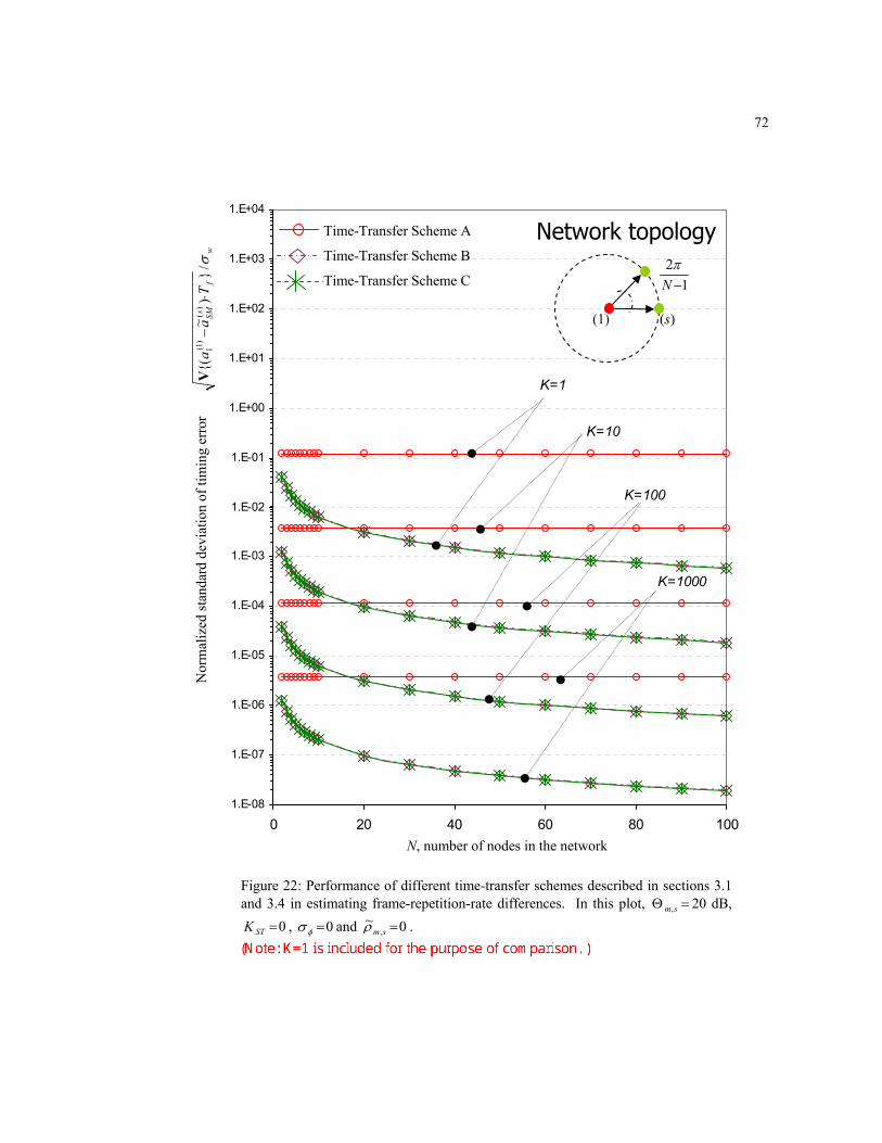
72
Figure 22: Performance of different time-transfer schemes described in sections 3.1 and 3.4 in estimating frame-repetition-rate differences. In this plot, =Θ sm, 20 dB,
0=STK , 0=φσ and 0~, =smρ .
1.E-08
1.E-07
1.E-06
1.E-05
1.E-04
1.E-03
1.E-02
1.E-01
1.E+00
1.E+01
1.E+02
1.E+03
1.E+04
0 20 40 60 80 100
K=1
K=10
K=100
K=1000
N, number of nodes in the network
Time-Transfer Scheme A
Time-Transfer Scheme B
Time-Transfer Scheme C
Nor
mal
ized
stan
dard
dev
iatio
n of
tim
ing
erro
r
12−Nπ
Network topology
(1) (s)
w
fs SM
Ta
aσ/
)~
()
()1( 1
⋅−
V
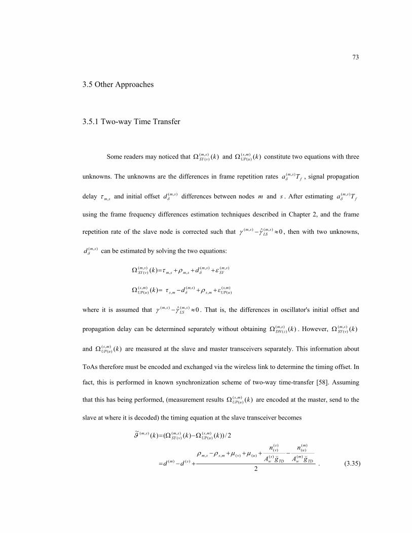
73
3.5 Other Approaches
3.5.1 Two-way Time Transfer
Some readers may noticed that )(),()( ksm
vSYΩ and )(),()( kms
uUPΩ constitute two equations with three
unknowns. The unknowns are the differences in frame repetition rates fsm Ta ),(
δ , signal propagation
delay sm,τ and initial offset ),( smdδ differences between nodes m and s . After estimating fsm Ta ),(
δ
using the frame frequency differences estimation techniques described in Chapter 2, and the frame
repetition rate of the slave node is corrected such that 0ˆ ),(),( ≈− smLS
sm γγ , then with two unknowns,
),( smdδ can be estimated by solving the two equations:
),(),(,,
),()( )( sm
SYsm
smsmsmvSY dk ερτ δ +++=Ω
)()(,
)(,
),()( )( s,m
uUPmsm,sδms
msuUP εdτk ++−=Ω ρ
where it is assumed that 0ˆ ),(),( ≈− smLS
sm γγ . That is, the differences in oscillator's initial offset and
propagation delay can be determined separately without obtaining )(),()( ksm
zDNΩ . However, )(),()( ksm
vSYΩ
and )(),()( kms
uUPΩ are measured at the slave and master transceivers separately. This information about
ToAs therefore must be encoded and exchanged via the wireless link to determine the timing offset. In
fact, this is performed in known synchronization scheme of two-way time-transfer [58]. Assuming
that this has being performed, (measurement results )(),()( kms
uUPΩ are encoded at the master, send to the
slave at where it is decoded) the timing equation at the slave transceiver becomes
)35.3(.2
2/))()(()(~
)(
)()(
)(
)()(
)()(,,)()(
),()(
),()(
),(
TDm
w
mu
TDs
w
sv
uvmssmsm
msuUP
smvSY
sm
gA
n
gA
n
dd
kkk
(( −+++−
+−=
Ω−Ω=
µµρρ
ϑ

74
The process described in the previous paragraph, commonly known as two-way time transfer
[58], can clearly be used to perform time-transfer as well and potentially supports more nodes in the
network with smaller timing jitter. The exchange of ToA measurement results could possibly be
provided by separate a communication channel (data channel) apart from the UWB channel dedicated
to time-transfer. If a narrowband channel is used, this entails additional hardware and power
requirement on the transceivers. If the information exchange is time division multiplexed into the
UWB channels, more time is needed than for transmitting downlink ranging pulses from the master to
slave nodes. In addition, if information is exchanged between transceivers using the TDMA UWB
channel, this would introduce additional latency that involves higher layer network protocol (encoding
and decoding of messages) that is hard to characterize for precision time-transfer.
The intention of this research is not to exchange encoded measurement results (time stamps)
for reasons cited in the previous paragraph. Nevertheless, the discussions on various time-transfer
architectures to follow are sufficiently generic to encompass (3.35). Ignoring the requirement of an
additional data channel, when compared to the two-way time-transfer, the proposed scheme described
earlier in section 3.1 has higher timing jitter. This is because the proposed scheme transmits an
additional slot of rK return timing pulses.
3.5.2 Returnable Timing System
If the oscillators in the network are coupled, instead of using explicit ToA measurement to
effect time-transfer, as described in [6], [34] and many earlier works, the performance analysis will be
different. For example, ignoring propagation delay and additive noise, the quantity investigated in [6]
is the oscillator timing process (denoted as ' kΘ ' in [6]), which corresponds to ( kfs kTT τ)()( + ) of
Chapter 1. The variable kτ is introduced to represent the adjustment made by the receiver when the
detector is placed inside a tracking loop. Using the principle of superposition

75
)())(1()()(ˆ)( )(
,1
)(,
)(f
sN
smmf
msmkf
s kTZHkTTZHkTTZ φατ zz −+⋅=+ ∑≠=
, (3.36)
where oZ denotes the Z-transform, )(zH is the transfer function of the phase locked loop and sm,α
is the gain of the system. Equation (3.36) is presented here for completeness and will not be pursued
further. Note that (3.36) illustrates the difference between the time synchronization techniques
described in [6] [34] and the proposed scheme in this research. In [6] and [34], a phase locked loop is
used to acquire the phase of the received narrowband signals with delay compensation to transfer time
from one node to another. In this case, )()( tT m and )()( tT s are manipulated directly. Further, in [34],
it is assumed that the drift of any individual oscillator is close to unity such that
smm
smm tTtT ,
)(,
)( )()( ττ +≈+ .
In the proposed SIN synchronization scheme, ToAs of the UWB monocycles are measured
directly. Then, for a network of nodes, it is more convenient mathematically to project )()( tT m and
)()( tT s onto t (the standard time scale, section 1.2). Hence the inverse mapping )()(
mkt and )(
)(skt of
fmk
m kTtT =)( )()(
)( and fsk
s kTtT =)( )()(
)( are utilized. The objective of time-transfer remains the same.
In this Chapter, the synchronization scheme for the SIN was presented. When compared with
two-way time-transfer [58], the TDMA time-transfer schemes proposed in section 3.1 and 3.3 (time-
transfer schemes A, B and C) do not require additional resources to exchange measurement results
between pair of nodes (no separate data channel is needed). They are well suited for applications
when it is advantageous to perform synchronization on the physical layer with little or no involvement
from higher layer protocols.

76
CHAPTER IV
TIME-TRANSFER ARCHITECTURES
In a network of wireless nodes, the timing of one node can be transferred to another using
different time-transfer structures/architectures [7] [34] [45].
In this Chapter, the master-slave (SM) architecture, with a designated master node and other
nodes in the network are slave nodes, is first introduced and analyzed. It is followed by description of
the hierarchical master-slave (HM) and the mutually synchronous (MU) time-transfer architectures.
The proposed MU and HM time-transfer networks are realized based on the "roving master" concept.
In the roving master concept, each node in the network takes its turn as the master node. To start the
time transfer, a node in the network is designated as the lead master node. The lead master node will
be the first node to start transferring its timing to other nodes in the network. The purpose of roving
the master duties is to avoid NLoS network signal propagation between nodes. In this research, nodes
in the network are assumed to be stationary during time transfer.
To analyze the performance of a SIN implemented with different time-transfer architectures,
we select to analyze only the case in which ToA measurements are obtained from an open loop timing
detector, i.e., the timing detector is not embedded in a tracking loop and the oscillator is free running
during synchronization. We will make use of the results presented earlier in Chapter 3 to analyze the
performance of the SIN.
In Chapter 3, sections 3.1 and 3.4, three different time-transfer schemes are presented. They
are time-transfer schemes A, B and C. In this Chapter, the estimation errors of individual nodes in a
network of N nodes after time-transfer are expressed as a function of ),(ˆ smdδ , ),(ˆ
smd
ε and ),( smLSγε given
in Chapter 3. Thus, by substituting time-transfer characteristic functions )(kθ of different time-
transfer schemes, the performance of the SIN for different time-transfer architectures utilizing
different time-transfer schemes can be readily obtained.

77
4.1 Master-Slave Time-Transfer Architecture
The time-transfer schemes described in Chapter 3 seek to transfer the initial offset and frame
repetition rate of the master node's oscillator to a slave node. If node 1 in a network of N nodes is the
sole master node, and time transfer occurs pair-wise between node 1 with other nodes in the network
using different time slots, a master-slave time-transfer architecture using time division multiple access
(TDMA) is realized. The necessity of a TDMA instead of a FDMA (Frequency Divisional Multiple
Access) scheme arises from the fact that we assume UWB impulse signal occupies all the available
bandwidth. It is well known that the timing resolution of a signal is inversely proportional to the
signal bandwidth.
A flow chart illustrating the single-master-to-multiple-slaves (SM) time-transfer architecture
is shown in Fig. 23. The objective of this architecture is to align the timing of slaves to that of the
designated master node.
Equations in section 3.3 express the variances in estimating the differences in initial offset
and frame repetition rate between the master and each slave node in the network. The subscripts in
these equations indicate that these measurements are obtained from the thv frame-synchronization
pulse, the thu pulse in uplink slot j and the thz pulse in down-link slot i of the slave transceiver.
That is, the slave node uses up-link slot j to transmit to the master and the master uses down-link slot
i to transmit to the slave during two-way ranging. The superscript ),( sm is used to indicate that the
measured ToAs are a function of the communication channel between the master m and slave node s
participating in the time-transfer.
In this research, we restrict ourselves to analyzing only the case when ToA measurements are
obtained from an open loop timing detector, i.e., it is assumed that the timing detector is not
embedded in a tracking loop and the oscillator is free running during time-transfer.

78
After the master node broadcast synchronization pulses to the slave nodes during the frame-
synchronization time slot, each slave node, using LS estimator, estimates the difference in pulse
repetition rate between its clock and the master node's clock, and adjusts its frame repetition rate to
that of the master. The difference in its initial offset is estimated by taking the sample mean of the
timing differences obtained after two-way ranging.
The variance in estimating the difference in oscillator frame repetition rate is given by (2.47)
while variance in estimating difference in initial offset is given by (3.24c). For ease of reference, they
are reproduced here
|ˆ| ),(2),(),(2ˆ ),(
smsmLS
smLSsm
LSγγ
εγγσ VΕ =−= ,
.))((
ˆ ),(),(2
21
0),( smsm
K
kST
smLSK
Kkd ϑγδ εε
θVVV +⋅
−
=∑−
=
Denoting the "settled" estimate of the initial offset and drift at node s , 1≠s , after time
transfer by )(~ sSMd and )(~ s
SMa respectively, we have
fss
LSfs
SM TaTa )(1
),1()( ˆ~ +=⋅ γ , (4.1a)
b)1.4(.~
ˆ~
),1(ˆ,1
)1(
)(),1()(
sds
sssSM
d
ddd
ερδ
++=
+=
Therefore the variances of the estimation errors )~( )()1(1
sSMaa − and )
~( )()1( s
SMdd − are given by
~ ),1()()1(1
ssSM LS
aa γεVV =− , (4.2a)
ˆ~
),1()()1( ssSM ddd δVV =− . (4.2b)
The expectation of the square of the difference in initial offset is
2,1
)()1(2)()1( ~~
)~
( ss
SMs
SM dddd ρ+−=− VΕ . (4.3)
The LS estimate ),1(ˆ sLSγ of the difference in frame repetition rate between node 1 and node s is not
affected by sm,~ρ .
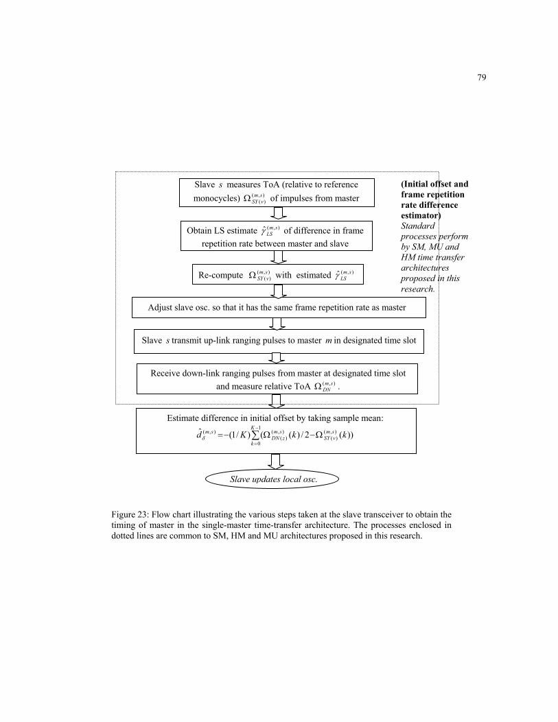
79
Slave updates local osc.
Slave s measures ToA (relative to reference monocycles) ),(
)(smvSYΩ of impulses from master
Obtain LS estimate ),(ˆ smLSγ of difference in frame
repetition rate between master and slave
Re-compute ),()(
smvSYΩ with estimated ),(ˆ sm
LSγ
Adjust slave osc. so that it has the same frame repetition rate as master
Slave s transmit up-link ranging pulses to master m in designated time slot
Receive down-link ranging pulses from master at designated time slot and measure relative ToA ),( sm
DNΩ .
Estimate difference in initial offset by taking sample mean:
∑−
=Ω−Ω−=
1
0
),()(
),()(
),( ))(2/)(()/1(ˆ K
k
smvSY
smzDN
sm kkKdδ
(Initial offset and frame repetition rate difference estimator) Standard processes perform by SM, MU and HM time transfer architectures proposed in this research.
Figure 23: Flow chart illustrating the various steps taken at the slave transceiver to obtain the timing of master in the single-master time-transfer architecture. The processes enclosed in dotted lines are common to SM, HM and MU architectures proposed in this research.

80
It is mentioned in [66] that oscillator phase noise )(tϕ depends on the choice of the
oscillator, and the power spectral density of )(tϕ ( )(ωϕS ) is usually specified as single-side-band
noise in unit of dBc/Hz (dB relative to the oscillator carrier power in a 1 Hz bandwidth) and denoted
as £(f).
A quick survey of the frequency control literature reveals that there exist various models to
characterize the timing jitter of oscillator [14] [36] [42] [51]. The model presented in [36] [42] is
adopted in this work. From [42], the first order structure function and hence the oscillator phase noise
can be obtained from £(f). A technique is given in [44] to calculate the RMS (root-mean-squares)
timing jitter from £(f). Applying the technique shown in [44] to the values of £(f) tabulated in [49], a
FTS9500 (1993) precision oscillator operating at nominal oscillation frequency of 5 MHz has a RMS
timing jitter of 72.1 fs (this calculation is illustrated in Fig. 24). This is better than the "good" crystal
oscillator mentioned in [44] which has a RMS timing jitter of 6 ps. The 5 MHz oscillator is chosen
because it is mentioned in [65] that 5 MHz is one of the standard frequencies for military
communication and synchronization subsystems. Further, a study on enhancing the performance of a
CMOS LC oscillator is presented in [40]. The "period jitter"11 of the various enhanced CMOS LC
oscillator ranges from 491 fs to 51 fs. Thus it is reasonable to assume, at current oscillator
manufacture technology, oscillator timing jitter φσ ranges from 10-11 (for a cheap oscillator) to 10-15
(for an expansive oscillator).
The variances expressed by (4.2a) and (4.2b) are plotted in Figs. 25, 26 and 27 for various
values of K and N . The received UWB monocycle is modeled using the nth order derivative of a
Gaussian curve described in section 1.2.5 and [11] [12] , and we choose monocycle waveform )(twn ,
8=n , which has a spectrum that fits into the FCC indoor mask. In our analysis, the pulse width
11 In [40], "period jitter" is defined as 1 kk tt −+V where kt is the absolute instant in time of the kth positive
voltage transition of the oscillator output and okk ftt /1 1 =−+E .
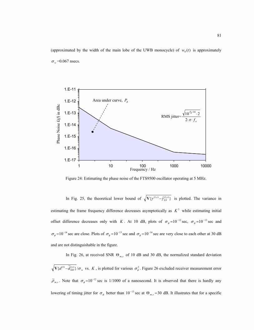
81
(approximated by the width of the main lobe of the UWB monocycle) of )(8 tw is approximately
wσ =0.067 nsecs.
In Fig. 25, the theoretical lower bound of ˆ ),1(),1( sLS
s γγ −V is plotted. The variance in
estimating the frame frequency difference decreases asymptotically as 3K while estimating initial
offset difference decreases only with K . At 10 dB, plots of 1210 −=φσ sec, 1310 −=φσ sec and
1410−=φσ sec are close. Plots of 1310−=φσ sec and 1410−=φσ sec are very close to each other at 30 dB
and are not distinguishable in the figure.
In Fig. 26, at received SNR sm,Θ of 10 dB and 30 dB, the normalized standard deviation
ws
SMdd σ/~
)()1( −V vs. K , is plotted for various 2φσ . Figure 26 excluded receiver measurement error
sm,~ρ . Note that 1210−=φσ sec is 1/1000 of a nanosecond. It is observed that there is hardly any
lowering of timing jitter for φσ better than 1310− sec at 30, =Θ sm dB. It illustrates that for a specific
Figure 24: Estimating the phase noise of the FTS9500 oscillator operating at 5 MHz.
Frequency / Hz
1.E-17
1.E-16
1.E-15
1.E-14
1.E-13
1.E-12
1.E-11
1 10 100 1000 10000
RMS jitter=o
P
f⋅⋅⋅
π
φ
2210 10/
Area under curve, φP
Phas
e N
oise
£(f)
in d
Bc

82
sm,Θ , when additive channel noise increases until 22 2),( φσσ >>smn , then the detector output variance
becomes ),(2),(),( 2222 smsmsm nnx σσσσ φ ≈+= , and an oscillator with even smaller phase noise would
not reduce the timing jitter significantly. That is, there is a threshold beyond which the variance in
estimating difference in initial offset is SNR limited. Conversely, when the oscillator phase noise is
much larger than additive channel noise, the variance in estimating difference in initial offset is
limited by oscillator timing jitter.
In Fig. 27, ws
SMdd σ/~
)()1( −V is plotted against number of nodes N in the network at
10, =Θ sm dB and 30, =Θ sm dB.
As illustrated in Figures 25, 26 and 27, the SM architecture is able to bring the standard
deviation of the difference in initial offset estimation to within one monocycle pulse width.
Figure 25: Theoretical lower bound on the standard deviation in estimating frame frequency difference between a pair of transceivers (N=2) as a function of K for various values of φσ at received SNR of Θm,s=10 dB and Θm,s=30 dB. Results obtained using time-transfer scheme A. The width of the UWB monocycle is approximately wσ =0.067 nsec.
30 dB
1.E-07
1.E-06
1.E-05
1.E-04
1.E-03
1.E-02
1.E-01
1.E+00
0 500 1000 1500 2000
1413 10,10 −−=φσ sec (AWGN limited)
1110−=φσ sec
141312 10,10,10 −−−=φσ sec (AWGN limited)
Number of frames, K
10 dB
1210−=φσ sec
w
sm LS
sm
σγ
γ/
ˆ
),
()
,(
−V
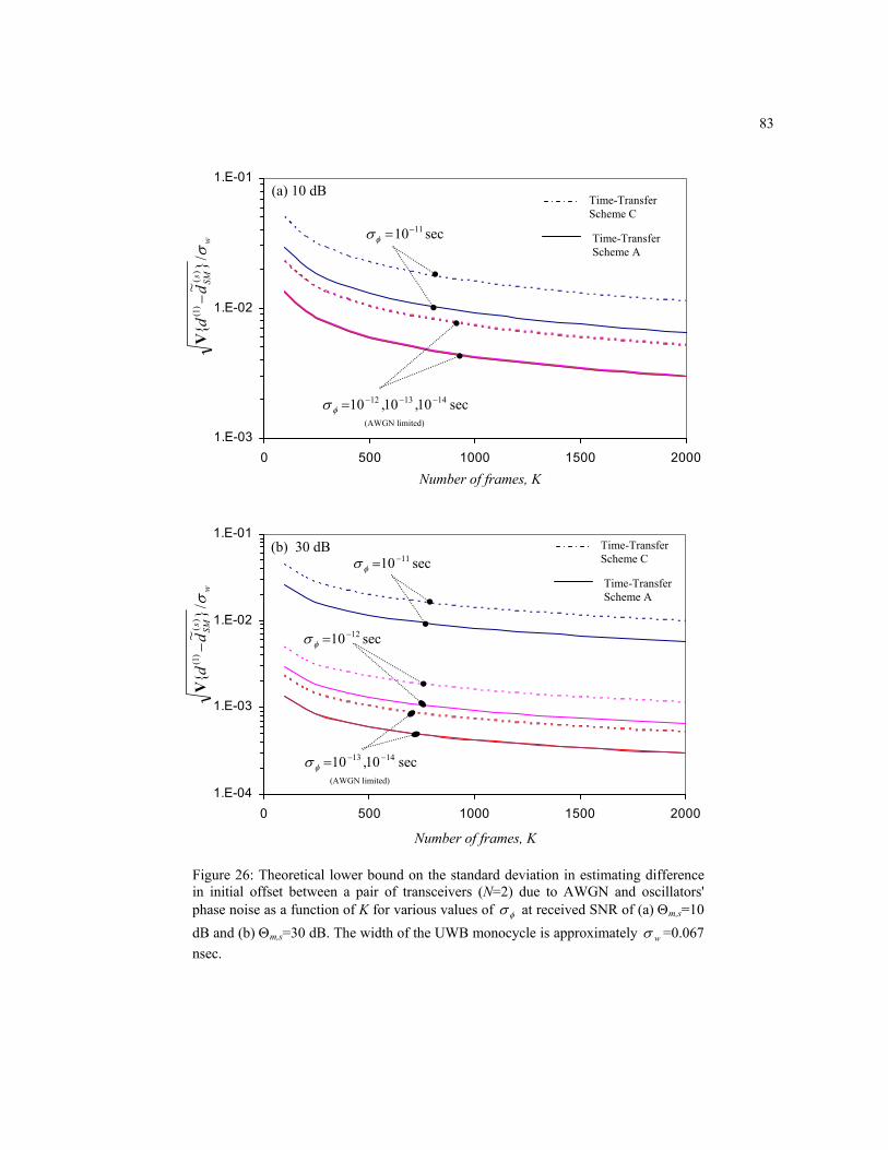
83
Figure 26: Theoretical lower bound on the standard deviation in estimating difference in initial offset between a pair of transceivers (N=2) due to AWGN and oscillators' phase noise as a function of K for various values of φσ at received SNR of (a) Θm,s=10 dB and (b) Θm,s=30 dB. The width of the UWB monocycle is approximately wσ =0.067 nsec.
1.E-03
1.E-02
1.E-01
0 500 1000 1500 2000
1110−=φσ sec
141312 10,10,10 −−−=φσ sec
(AWGN limited)
Number of frames, K
Time-Transfer Scheme C
Time-Transfer Scheme A
w
sSMd
dσ/
~
)(
)1(−
V
(a) 10 dB
1.E-04
1.E-03
1.E-02
1.E-01
0 500 1000 1500 2000
1210 −=φσ sec
1110 −=φσ sec
1413 10,10 −−=φσ sec (AWGN limited)
Time-Transfer Scheme C
Time-Transfer Scheme A
w
sSMd
dσ/
~
)(
)1(−
V
Number of frames, K
(b) 30 dB
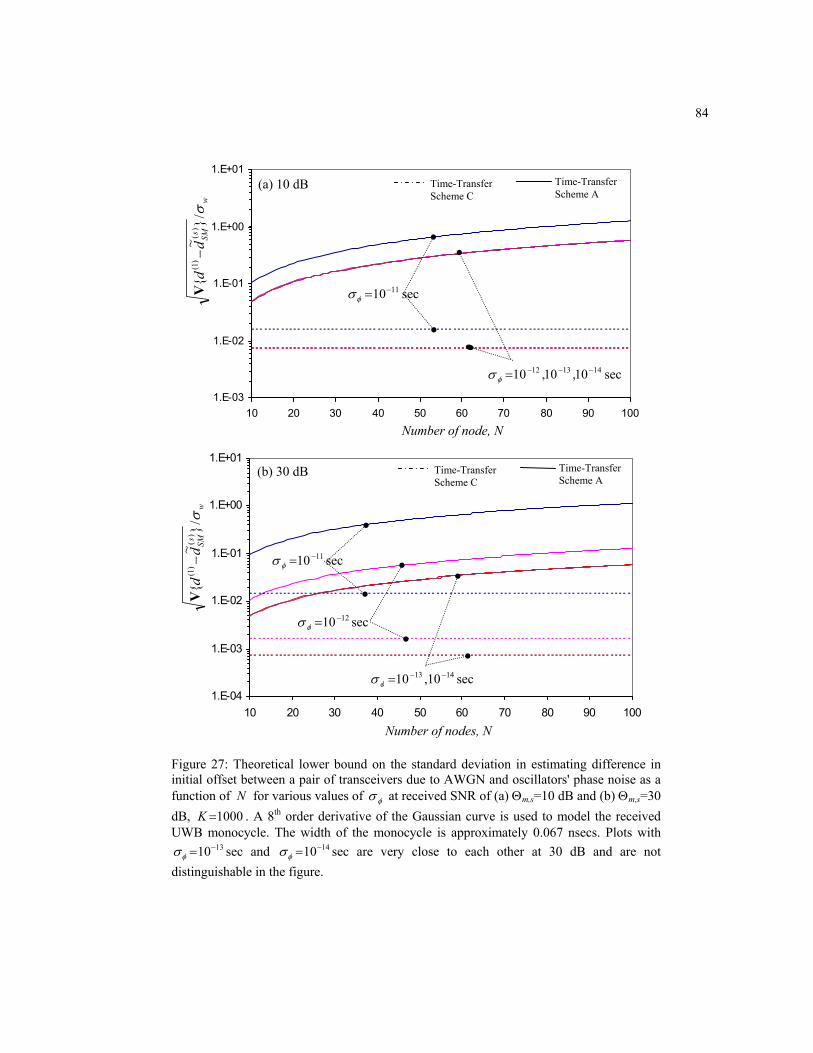
84
Figure 27: Theoretical lower bound on the standard deviation in estimating difference in initial offset between a pair of transceivers due to AWGN and oscillators' phase noise as a function of N for various values of φσ at received SNR of (a) Θm,s=10 dB and (b) Θm,s=30 dB, 1000=K . A 8th order derivative of the Gaussian curve is used to model the received UWB monocycle. The width of the monocycle is approximately 0.067 nsecs. Plots with
1310−=φσ sec and 1410−=φσ sec are very close to each other at 30 dB and are not distinguishable in the figure.
1.E-03
1.E-02
1.E-01
1.E+00
1.E+01
10 20 30 40 50 60 70 80 90 100
1110−=φσ sec
141312 10,10,10 −−−=φσ sec
Number of node, N
w
sSMd
dσ/
~
)(
)1(−
V Time-Transfer
Scheme C Time-Transfer Scheme A
(a) 10 dB
1.E-04
1.E-03
1.E-02
1.E-01
1.E+00
1.E+01
10 20 30 40 50 60 70 80 90 100
1110 −=φσ sec
1210 −=φσ sec
Number of nodes, N
w
sSMd
dσ/
~
)(
)1(−
V
(b) 30 dB Time-Transfer Scheme C
Time-Transfer Scheme A
1413 10,10 −−=φσ sec
85
4.2 Roving Masters
The concept of a "roving" master, which is builds upon the master-slave time-transfer, is to
let each transceiver in the network take a turn as the master node. The purpose of this approach is to
extend the geographical coverage (Fig. 28a) of the synchronous network and to overcome blockages
in signal propagation paths (Fig. 28b).
In wireless sensor networks, the wireless nodes are usually of small form factor with limited
power. Therefore the transmission range of each node is likely to be limited due to power constraint.
The roving master concept works much like a terrestrial cellular system with numerous fixed base
stations each covering a small local area. Each node in the SIN is capable of being the master (base
station) to communicate its timing to other nodes (slaves ≡ mobile terminals) that are in close
proximity with it. It first synchronized itself to the timing of a designated lead-master node, i.e., the
node that is tasked to start the synchronization process as the first master node. When it becomes the
master, it propagates this timing to other nodes that the lead-master on its own cannot reach. Thus
roving the master increases the coverage of the network. The synchronous network's coverage,
accumulated timing jitter in individual nodes and accuracy of time-transfer, depends very much on the
scheduling scheme of the roving masters and the geographical layout of nodes in the network
(network topology) as will be illustrated in the following sections.
As pointed out earlier, the proposed synchronization scheme, like other wireless systems that
rely on measuring the ToA of signals, its performance is limited by the present of NLoS
measurements error that can significantly degrade the accuracy of the time-transfer. The roving master
concept introduces diversity by exploiting the redundancy inherent in the network. As illustrated in
Fig. 28b, node 'C' can choose from either node 'A' or 'B' or a soft combination of timing information
from both nodes to establish synchronization with the network. The possibility that a clear LoS exists,
which the nodes rely on for accurate time-transfer, between any pair of nodes (one of them is the
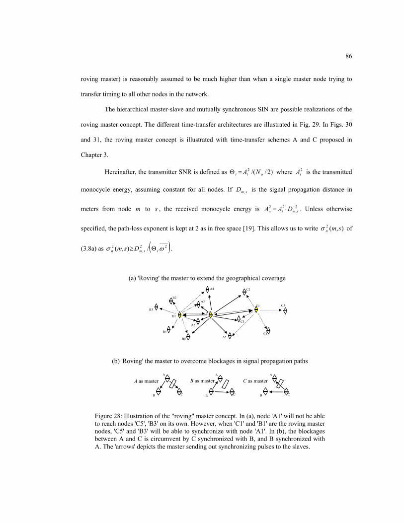
86
roving master) is reasonably assumed to be much higher than when a single master node trying to
transfer timing to all other nodes in the network.
The hierarchical master-slave and mutually synchronous SIN are possible realizations of the
roving master concept. The different time-transfer architectures are illustrated in Fig. 29. In Figs. 30
and 31, the roving master concept is illustrated with time-transfer schemes A and C proposed in
Chapter 3.
Hereinafter, the transmitter SNR is defined as )2//(2ott NA=Θ where 2
tA is the transmitted
monocycle energy, assuming constant for all nodes. If smD , is the signal propagation distance in
meters from node m to s , the received monocycle energy is 2,
22 −⋅= smtw DAA . Unless otherwise
specified, the path-loss exponent is kept at 2 as in free space [19]. This allows us to write ),(2 smnσ of
(3.8a) as ( )22,
2 /),( ωσ tsmn Dsm Θ≥ .
(a) 'Roving' the master to extend the geographical coverage
A1B1
C4
A3B2
C3A2
B4
C1
A4
B3 C5
A5B5
C2
Figure 28: Illustration of the "roving" master concept. In (a), node 'A1' will not be able to reach nodes 'C5', 'B3' on its own. However, when 'C1' and 'B1' are the roving master nodes, 'C5' and 'B3' will be able to synchronize with node 'A1'. In (b), the blockages between A and C is circumvent by C synchronized with B, and B synchronized with A. The 'arrows' depicts the master sending out synchronizing pulses to the slaves.
A
B C
A as master A
B C
B as master A
B C
C as master
(b) 'Roving' the master to overcome blockages in signal propagation paths
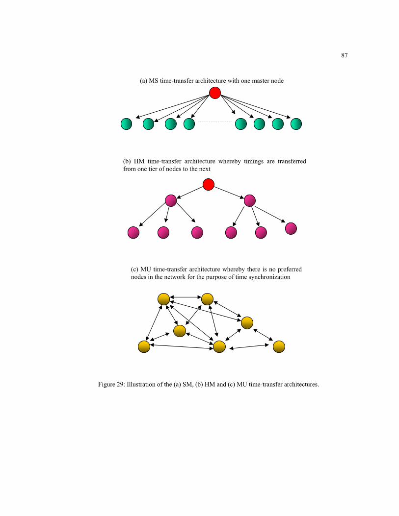
87
Figure 29: Illustration of the (a) SM, (b) HM and (c) MU time-transfer architectures.
(a) MS time-transfer architecture with one master node
(b) HM time-transfer architecture whereby timings are transferred from one tier of nodes to the next
(c) MU time-transfer architecture whereby there is no preferred nodes in the network for the purpose of time synchronization

88
Figure 30: Illustration of the time transfer activities at each node utilizing the roving master concept with time-transfer scheme A. In this example, there are N=3 nodes in the network and node 2 is the roving master node after node 1 has transferred its timing to nodes 2 and 3. There are K frames per time slot. For the purpose of illustration, the durations of all slot time are equal. In practice, due to difference in initial offset and frame repetition rate, the slot times of each node are of slightly different lengths.
Com
plet
ion
of o
ne ro
ving
mas
ter s
essio
n w
ith n
ode 1
as th
e mas
ter n
ode.
Dur
atio
n of
one
slo
t tim
e
1 br
oadc
asts
fram
e syn
. pul
ses
to al
l oth
er n
odes
1 re
ceiv
es u
plin
k pu
lses f
rom
2
1 re
ceiv
es u
plin
k pu
lses f
rom
3
1 tra
nsm
its
dow
nlin
k pu
lses
to 2
1 tra
nsm
its
dow
nlin
k pu
lses
to 3
Nod
e 2 ta
kes o
ver a
s the
ro
ving
mas
ter.
K ST=
(2N
- 1)K
, whe
re N
=3.
Star
ts of
tim
e sy
nchr
oniz
atio
n,
K ST=
0
In M
U, n
ode 1
will
rece
ive t
he fr
ame s
yn.
pulse
s fro
m n
ode 2
to ac
quire
the t
imin
g of
no
de 2
. In
HM
, it w
ill n
ot p
artic
ipat
e fur
ther
in
the t
ime s
ynch
roni
zatio
n pr
oces
s.
t
2 re
ceiv
es
dow
nlin
k pu
lses
from
1
2 re
ceiv
es fr
ame
syn.
pul
ses f
rom
1
2 tra
nsm
its
uplin
k pu
lses t
o 1
2
rece
ives
upl
ink
pulse
s fro
m 3
2
broa
dcas
ts fra
me s
yn. p
ulse
s
t
3 re
ceiv
es
dow
nlin
k pu
lses
from
1
3 re
ceiv
es fr
ame
syn.
pul
ses f
rom
1
3 tra
nsm
its
uplin
k pu
lses t
o 2
3 tra
nsm
its
uplin
k pu
lses t
o 1
3
rece
ives
fram
e sy
n. p
ulse
s fro
m
2
t

89
Com
pleti
on of
one r
ovin
g mas
ter se
ssio
n with
node
1 as
the m
aster
node
.
Dura
tion o
f one
fra
me t
ime
Node
2 tak
es ov
er as
the
rovi
ng m
aster
. K S
T=(2
N - 1
)K, w
here
N=3
. St
arts
of ti
me
sync
hron
izatio
n, K S
T=0
In M
U, no
de 1
will
rece
ive t
he fr
ame s
yn.
pulse
s fro
m no
de 2
to ac
quire
the t
imin
g of
node
2. In
HM
, it w
ill no
t par
ticip
ate fu
rther
in
the t
ime s
ynch
roni
zatio
n pro
cess
.
t
Pair-
wise
tim
e-tra
nsfe
r rep
eated
Ktim
es
t t
syn. UP
UP DOWN
DOWN
syn. UP
UP DOWN
DOWN
syn. UP
UP DOWN
DOWN
UP syn.
DOWN
Figure 31: Illustration of the time transfer activities at each node utilizing the roving master concept with time-transfer scheme C. In this example, there are N=3 nodes in the network and node 2 is the roving master node after node 1 has transferred its timing to nodes 2 and 3. The pair-wise time-transfer is performed K times before next node take over as the roving master.
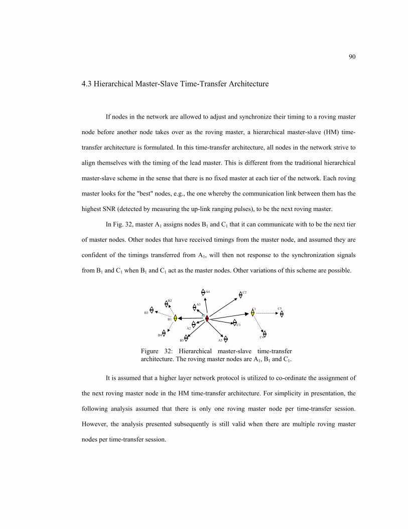
90
4.3 Hierarchical Master-Slave Time-Transfer Architecture
If nodes in the network are allowed to adjust and synchronize their timing to a roving master
node before another node takes over as the roving master, a hierarchical master-slave (HM) time-
transfer architecture is formulated. In this time-transfer architecture, all nodes in the network strive to
align themselves with the timing of the lead master. This is different from the traditional hierarchical
master-slave scheme in the sense that there is no fixed master at each tier of the network. Each roving
master looks for the "best" nodes, e.g., the one whereby the communication link between them has the
highest SNR (detected by measuring the up-link ranging pulses), to be the next roving master.
In Fig. 32, master A1 assigns nodes B1 and C1 that it can communicate with to be the next tier
of master nodes. Other nodes that have received timings from the master node, and assumed they are
confident of the timings transferred from A1, will then not response to the synchronization signals
from B1 and C1 when B1 and C1 act as the master nodes. Other variations of this scheme are possible.
It is assumed that a higher layer network protocol is utilized to co-ordinate the assignment of
the next roving master node in the HM time-transfer architecture. For simplicity in presentation, the
following analysis assumed that there is only one roving master node per time-transfer session.
However, the analysis presented subsequently is still valid when there are multiple roving master
nodes per time-transfer session.
A1B1
C4
A3B2
C3A2
B4
C1
A4
B3 C5
A5B5
C2
Figure 32: Hierarchical master-slave time-transfer architecture. The roving master nodes are A1, B1 and C1.
91
A feasible HM network works as follows. Assuming ),(),(ˆ smsmLS γγ ≈ , so that )(),(
)( kmsuUPΩ and
)(),()( ksm
zDNΩ are approximately independent of time index k , the current roving master m chooses the
next roving master 'm so that
)(minarg' ),()( km ms
uUPsΩ= V , (4.4a)
where
2),(),()(
),()( )()( ukk smms
uUPms
uUP LS⋅+=Ω γεε VVV , (4.4b)
and 'm acquires the timing of the previous roving master m .
At the end of synchronization, slave s has measurements of )(),()( ksm
zDN′Ω from all roving
master nodes m′ , the cardinality of m′ not necessary equals 1−N . The slave s , not one of the
roving masters, will use the corresponding ),(ˆ smdδ , ),(ˆ smLSγ computed from the roving master m where,
)(minarg ),'()( km sm
zDNmΩ=
′V , (4.5a)
to correct its transceiver oscillator. The variance )( ),()( ksm
zDN′ΩV , which is the variance of the ToA of
the downlink ranging pulse, is
.)()( 2),(),()(
),()( uzk smsm
zDNsm
zDN LS−⋅+=Ω γεε VVV (4.5b)
In arriving at (4.4b) and (4.5b), we have make use of the fact that,
c)5.4(.0
),(),()(
),(),()(
ΕΕΕ
=
⋅=⋅ smsmuUP
smsmuUP LSLS γγ εεεε
d)5.4(.0
),(),()(
),(),()(
ΕΕΕ
=
⋅=⋅ smsmzDN
smsmzDN LSLS γγ εεεε
This is because the zero mean noise processes ),()(
smuUPε , ),(
)(smzDNε and ),( sm
LSγε are present at different time
frames and therefore can be assumed to be statistically independent. Moreover noise processes present
during transmission between different pair of nodes (nodes are spatially distributed) can be assumed
to be independent too.
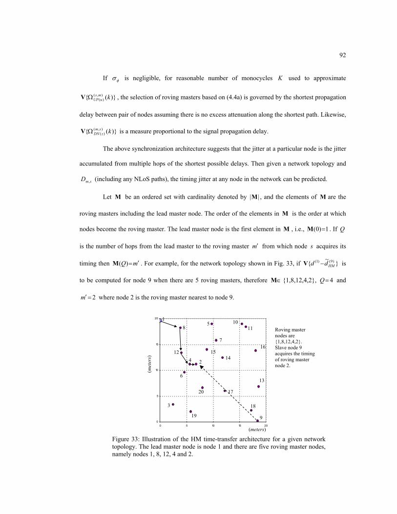
92
If φσ is negligible, for reasonable number of monocycles K used to approximate
)( ),()( kms
uUPΩV , the selection of roving masters based on (4.4a) is governed by the shortest propagation
delay between pair of nodes assuming there is no excess attenuation along the shortest path. Likewise,
)( ),()( ksm
zDNΩV is a measure proportional to the signal propagation delay.
The above synchronization architecture suggests that the jitter at a particular node is the jitter
accumulated from multiple hops of the shortest possible delays. Then given a network topology and
smD , (including any NLoS paths), the timing jitter at any node in the network can be predicted.
Let M be an ordered set with cardinality denoted by ||M , and the elements of M are the
roving masters including the lead master node. The order of the elements in M is the order at which
nodes become the roving master. The lead master node is the first element in Μ , i.e., 1)0( =Μ . If Q
is the number of hops from the lead master to the roving master m′ from which node s acquires its
timing then mQ ′=)(Μ . For example, for the network topology shown in Fig. 33, if ~
)9()1(HMdd −V is
to be computed for node 9 when there are 5 roving masters, therefore ∈Μ 1,8,12,4,2, 4=Q and
2=′m where node 2 is the roving master nearest to node 9.
Figure 33: Illustration of the HM time-transfer architecture for a given network topology. The lead master node is node 1 and there are five roving master nodes, namely nodes 1, 8, 12, 4 and 2.
0
5
10
15
20
0 5 10 15 20
1
2
3
4
5
6
7
8
9
10 11
12
13
14 15
16
17
18
19
20
(met
ers)
(meters)
Roving master nodes are 1,8,12,4,2. Slave node 9 acquires the timing of roving master node 2.

93
If )(~ sHMd and )(~ s
HMa denote the settled initial offset and drift at node s after hierarchical
master-slave time-transfer, we have
a)6.4(,~~
~
~ˆ~
)(1
))(),1(())(),1((
ˆ)),(()),((
ˆ)1(
),'(ˆ,'
)'(
),'(ˆ,'
)()'()(
),'()()(
M
MMMM
MM ∑
≠=
−− ++++=
++=
++−+=
+=
Q
sqq
qqqq
dsQsQ
d
smdsm
m
smdsm
sms
smssHM
d
d
ddd
ddd
ρερε
ερ
ερδ
b)6.4(.
ˆ~
)(,1
))(),1(()),(()1(1
),'()'(1
),'(),'()(1
),'()(1
)(
M
MMM ∑≠
=
−++=
+=
++=
+=
Q
sqq
qqsQf
smf
m
smsmf
s
smf
sf
sHM
LSLS
LS
LS
Ta
Ta
Ta
TaTa
γγ
γ
γ
δ
εε
ε
εγ
γ
This allows us to express the variance of the difference )~
( )()1( sHMdd − as
,))((
))12()((
ˆˆ
~
)(,1
))(),(())(),1((2
21
0
)),(()),((2
21
0
)(,1
))(),1(()),((
)(,1
))(),1((ˆ
)),((ˆ
)()1(
∑∑
∑
∑
∑
≠=
−
−
=
−
=
≠=
−
≠=
−
+⋅
−
+
+⋅
⋅⋅−−
=
+=
+=−
Q
sqMq
qqqq
K
kST
sQsQ
K
k
Q
sqMq
qqsQ
Q
sqMq
qMqMd
sQMd
sHM
LS
LS
K
Kk
K
QKNk
dd
dd
MMMM
MM
MMM
VV
VV
VV
VVV
ϑγ
ϑγ
δδ
εεθ
εεθ
εε
where )1()12( −⋅⋅−= qKNKST and
,/)(
~
),1(2),1(21
0
),1(ˆ
)()1(
ssK
k
sd
sHM
Kk
dd
LS ϑγ εεθ
ε
VV
VV
+⋅
=
=−
∑−
=
where K
mssm xxsm
4),(),(5
22
),( σσεϑ
+⋅=V and 222
,2 2/),( φσωσ +Θ= tsmx Dsm .
for 0>Q (4.7a)
for 0=Q (4.7b)
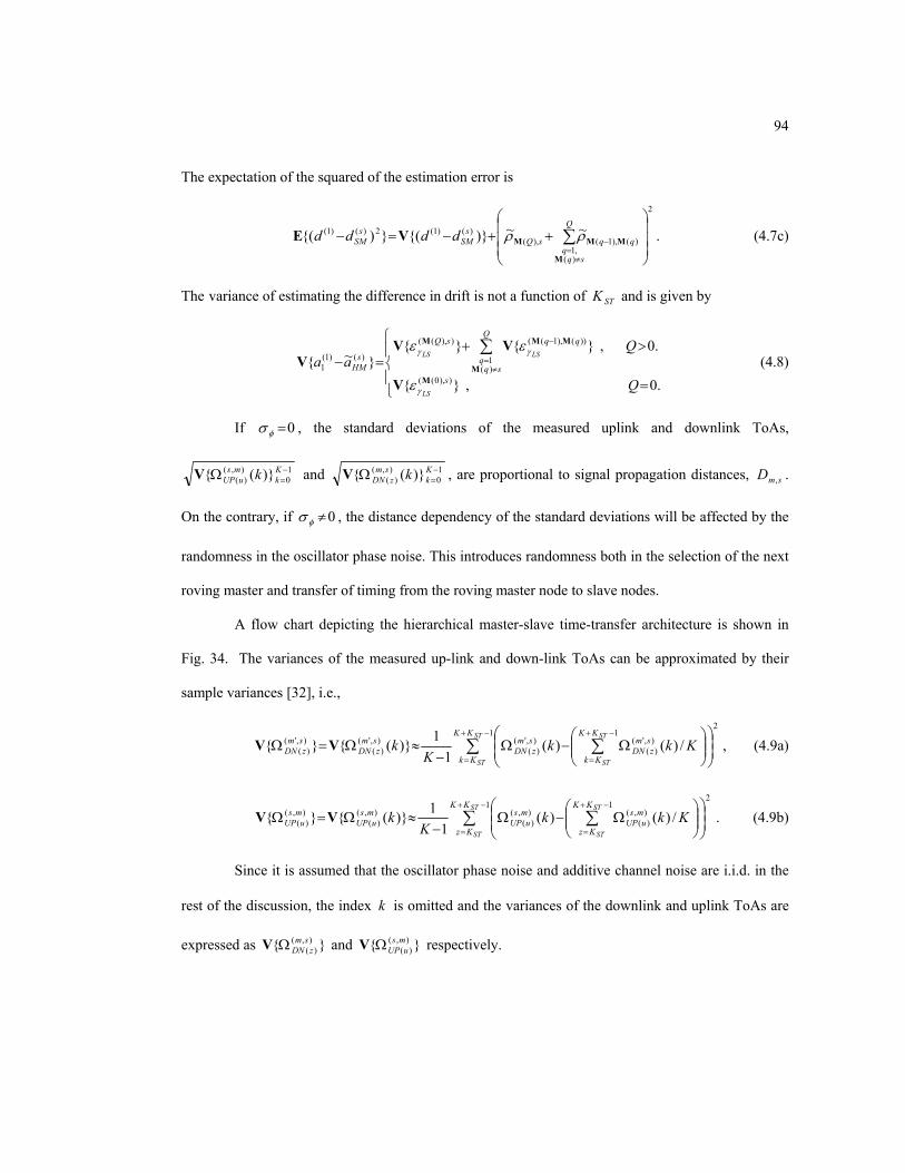
94
The expectation of the squared of the estimation error is
2
)(,1
)(),1(),()()1(2)()1( ~~)()(
++−=− ∑
≠=
−
Q
sqq
qqsQs
SMs
SM ddddM
MMMVΕ ρρ . (4.7c)
The variance of estimating the difference in drift is not a function of STK and is given by
=
>+=−
∑≠
=
−
.0,
.0,~
)),0(()(1
))(),1(()),((
)()1(1
Q
Qaa
s
Q
sqq
qqsQ
sHM
LS
LSLS
ΜM
MΜΜ
V
VVV
γ
γγ
ε
εε (4.8)
If 0=φσ , the standard deviations of the measured uplink and downlink ToAs,
10
),()( )( −
=Ω Kk
msuUP kV and 1
0),(
)( )( −=Ω K
ksm
zDN kV , are proportional to signal propagation distances, smD , .
On the contrary, if 0≠φσ , the distance dependency of the standard deviations will be affected by the
randomness in the oscillator phase noise. This introduces randomness both in the selection of the next
roving master and transfer of timing from the roving master node to slave nodes.
A flow chart depicting the hierarchical master-slave time-transfer architecture is shown in
Fig. 34. The variances of the measured up-link and down-link ToAs can be approximated by their
sample variances [32], i.e.,
∑ ∑−+
=
−+
=
Ω−Ω
−≈Ω=Ω
12
1),'()(
),'()(
),'()(
),'()( /)()(
11)(
ST
ST
ST
ST
KK
Kk
KK
Kk
smzDN
smzDN
smzDN
smzDN Kkk
KkVV , (4.9a)
∑ ∑−+
=
−+
=
Ω−Ω
−≈Ω=Ω
12
1),()(
),()(
),()(
),()( /)()(
11)(
ST
ST
ST
ST
KK
Kz
KK
Kz
msuUP
msuUP
msuUP
msuUP Kkk
KkVV . (4.9b)
Since it is assumed that the oscillator phase noise and additive channel noise are i.i.d. in the
rest of the discussion, the index k is omitted and the variances of the downlink and uplink ToAs are
expressed as ),()(
smzDNΩV and ),(
)(ms
uUPΩV respectively.
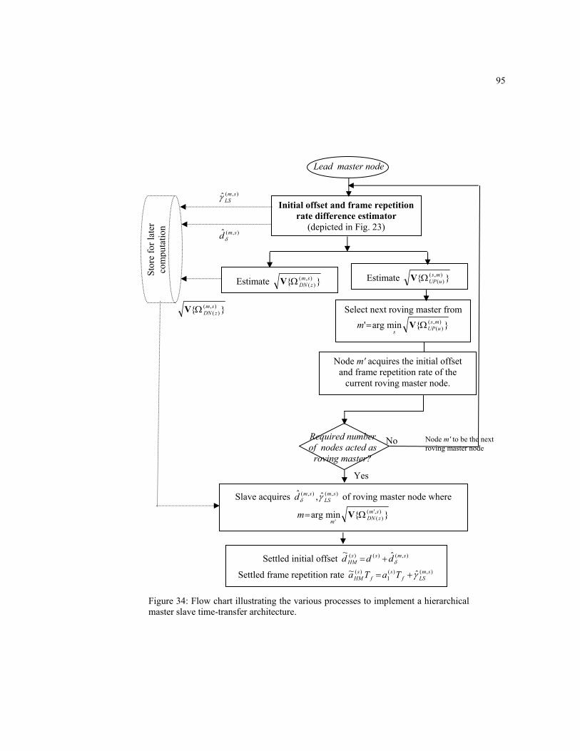
95
),()(
smzDNΩV
Required number of nodes acted as
roving master?
Lead master node
Initial offset and frame repetition rate difference estimator
(depicted in Fig. 23)
Estimate ),()(
smzDNΩV
Stor
e fo
r lat
er
com
puta
tion
Select next roving master from minarg' ),(
)(ms
uUPsm Ω= V
Yes
No
),(ˆ smdδ
Settled initial offset ),()()( ˆ~ smssHM ddd δ+=
Settled frame repetition rate ),()(1
)( ˆ~ smLSf
sf
sHM TaTa γ+=
Figure 34: Flow chart illustrating the various processes to implement a hierarchical master slave time-transfer architecture.
Estimate ),()(
msuUPΩV
Slave acquires ),(),( ˆ,ˆ smLS
smd γδ of roving master node where
minarg ),'()('
smzDNm
m Ω= V
),(ˆ smLSγ
Node m' acquires the initial offset and frame repetition rate of the
current roving master node.
Node m' to be the next roving master node

96
4.4 Mutually Synchronous Time-Transfer Architecture
The synchronous networks describe in sections 4.1 and 4.3 employ a master-slave
synchronization scheme where nodes in the network align their timings to a designated master node.
In this section, the mutually synchronous time-transfer architecture is introduced.
If there are N nodes in a network, a single synchronization session of master-slave will take
))1(2( sr KKN +− time frames. A complete roving of all N transceivers in the network will take
NKN )12( − time frames if KKK rs == . More importantly, at the end of one roving cycle, each
transceiver in the network would have obtained )1( −N measurements of 10
),()( )( −
=Ω Kk
smvSY k ,
10
),()( )( −
=Ω Kk
smzDN k and 1
0),()( )( −
=Ω Kk
msuUP k . If appropriate ToA measurement is weighted [34] according to
some criteria such as received signal strength, the timing adjustments at each node can be obtained
using a weighted combination of inputs from all other nodes in the network. Thus we have a MU
network, which is characterized by every oscillator in the network contributing to the settled timing of
the network.
If the approaches described in section 3.3 are used to estimate ),( smdδ (3.24a) and ),( smγ is
estimated using the LS estimator described by (2.43e), a MU scheme maybe implemented as follows.
Assuming nodes act as master in a natural order, i.e., node 1 is the first roving master node,
follows by node 2, node 3, …etc. Whenever a node s is not a roving master, it computes ),'()(
smzDNΩV ,
acquires the frame repetition rate of m′ and estimates ),'(ˆ smdδ . For example, if there are 3 nodes
1,2,3 in the network, when node 1 is the master, 2 and 3 acquire 1's frame repetition rate. When 2
becomes the roving master, 1 has to acquire the frame repetition rate of 2, which is a noisy copy of its
original frame repetition rate. When 3 is the roving master, it transfers its frame repetition rate, which
3 has earlier acquired from 2, to 1. Preceding initial offset estimation with pair-wise frame repetition
rate estimation is to minimize ˆ ),'( smdδV . Thus all nodes in the network will have a noisy copy of the
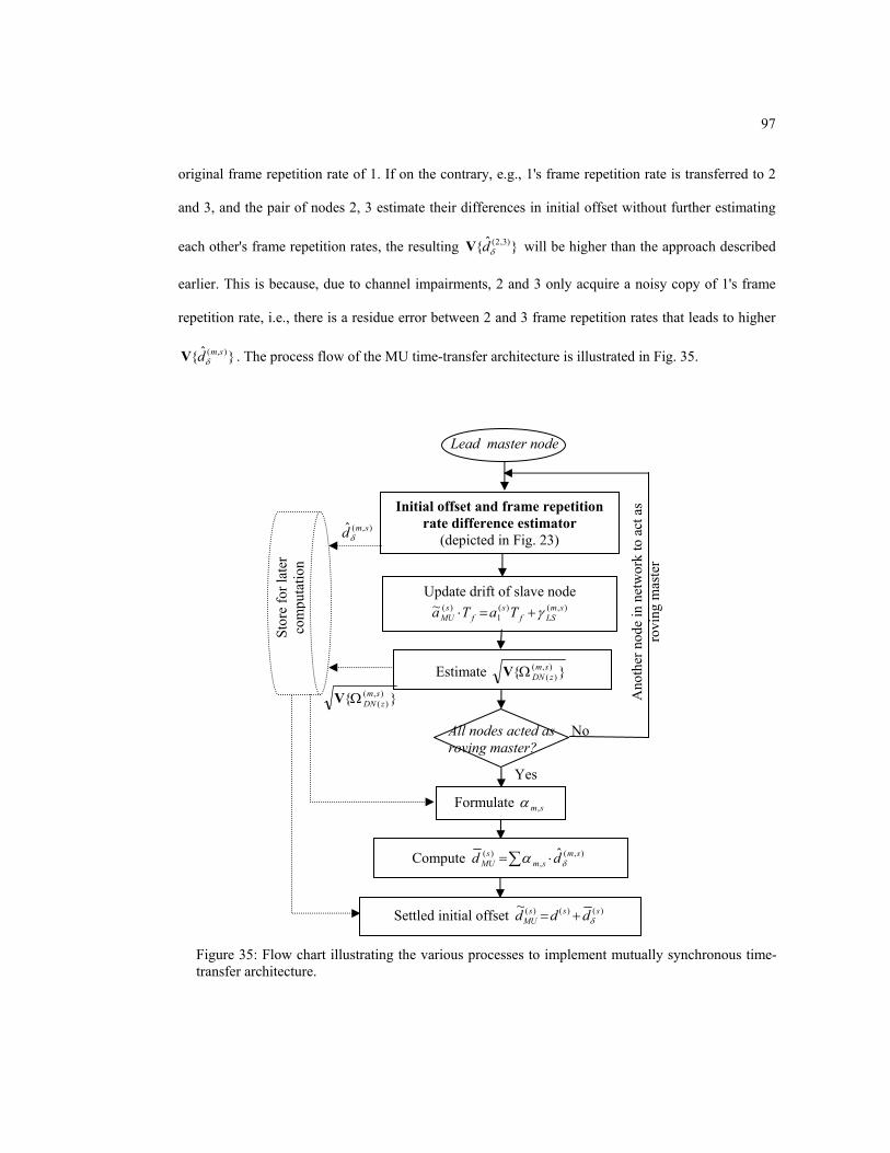
97
original frame repetition rate of 1. If on the contrary, e.g., 1's frame repetition rate is transferred to 2
and 3, and the pair of nodes 2, 3 estimate their differences in initial offset without further estimating
each other's frame repetition rates, the resulting ˆ )3,2(δdV will be higher than the approach described
earlier. This is because, due to channel impairments, 2 and 3 only acquire a noisy copy of 1's frame
repetition rate, i.e., there is a residue error between 2 and 3 frame repetition rates that leads to higher
ˆ ),( smdδV . The process flow of the MU time-transfer architecture is illustrated in Fig. 35.
),()(
smzDNΩV
All nodes acted as roving master?
Lead master node
Initial offset and frame repetition rate difference estimator
(depicted in Fig. 23)
Estimate ),()(
smzDNΩV
Stor
e fo
r lat
er
com
puta
tion
Formulate sm,α
Yes
No
),(ˆ smdδ
Compute ∑ ⋅= ),(,
)( ˆ smsm
sMU dd δα
Settled initial offset )()()(~ sssMU ddd δ+=
Figure 35: Flow chart illustrating the various processes to implement mutually synchronous time-transfer architecture.
Update drift of slave node ),()(
1)(~ sm
LSfs
fs
MU TaTa γ+=⋅
Ano
ther
nod
e in
net
wor
k to
act
as
rovi
ng m
aste
r

98
Let the settled drift of node s be )(~ sMUa . From the description of pair-wise time transfer
presented in the previous paragraphs, )(~ sMUa is given by
)10.4(,
~
),(1
1
)1,()1(1
),(),1()6,5()5,4()4,3()3,2()2,1()1()(1
sNN-
n
nnf
sNNNff
sMU
LSLS
LSLSLSLSLSLSLS
Ta
TaTa
γγ
γγγγγγγ
εε
εεεεεεε
++=
++++++++=
∑=
+
−L
where the random variable ),( smLSγε is the LS estimation error when estimating ),( smγ . Further, the
square of (4.10) is
( ) ( ) ( )
+⋅⋅++
+= ∑∑
=
+
=
+1
1
)1()1(1
),(2),(2
1
)1,()1(1
2)( //2//~ N-
nf
n,nγf
sNf
sNN
nf
nnsMU TεaTTTaa
LSLSLSLS γγγ εεε1-
. (4.11)
Therefore
)1(1
)( ~ aa sMU =Ε , (4.12a)
and
( )
b)12.4(,//)(
//~
)(1
1
)1(2)1(1
)(21
1
)1()1(1
2)(
VV
VVΕΕ
fN,sγ
N-
nf
n,nγ
fN,sγ
N-
nf
n,nγ
sMU
TεTεa
TεTεaa
LSLS
LSLS
++=
+
+=
∑
∑
=
+
=
+
( ) ( )
c)12.4(.//
~~~
)(1
1
)1(
2)(2)()(
VV
ΕΕV
fN,sγ
N-
nf
n,nγ
sMU
sMU
sMU
TεTε
aaa
LSLS+=
−=
∑=
+
Here the sample variance of the settled drift estimate across all nodes in the network, denoted by
~ MUaV , after time synchronization is of interest. The variance ~ MUaV is defined to be the sample
variance [32] of )(~ sMUa , Ns ,...,1= , and mean of ~ MUaV is defined as
−
−= ∑ ∑
= =
N
s
N
s
sMU
sMUMU a
Na
Na
1
2
1
)()( ~1~1
1~ ΕV . (4.13a)
The quantity ∑=
N
s
sMU Na
1
)( /~ is known as the sample mean. It is derived in Appendix B that
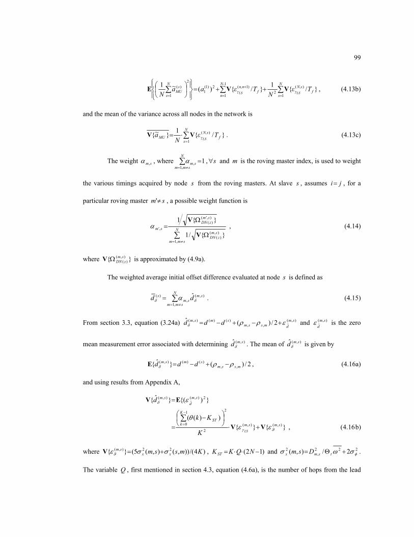
99
∑∑∑==
+
=++=
N
sf
N,sγ
N-
nf
n,nγ
N
s
sMU Tε
NTεaa
N LSLS1
)(2
1
1
)1(2)1(1
2
1
)( /1/)(~1 VVΕ , (4.13b)
and the mean of the variance across all nodes in the network is
∑=
⋅=N
sf
N,sγMU Tε
Na
LS1
)( /1~ VV . (4.13c)
The weight sm,α , where 1,1
, =∑≠=
N
smmsmα , s∀ and m is the roving master index, is used to weight
the various timings acquired by node s from the roving masters. At slave s , assumes ji= , for a
particular roving master sm ≠' , a possible weight function is
,/1
1
,1
),()(
),'()(
,'
∑≠=
Ω
Ω=
N
smm
smzDN
smzDN
sm
V
Vα (4.14)
where ),()(
smzDNΩV is approximated by (4.9a).
The weighted average initial offset difference evaluated at node s is defined as
∑≠=
=N
smm
smsm
s dd,1
),(,
)( ˆδδ α . (4.15)
From section 3.3, equation (3.24a) ),(ˆ,,
)()(),( 2/)(ˆ smdmssm
smsm ddd ερρδ +−+−= and ),(ˆ
smd
ε is the zero
mean measurement error associated with determining ),(ˆ smdδ . The mean of ),(ˆ smdδ is given by
2/)(ˆ ,,)()(),(
mssmsmsm ddd ρρδ −+−=Ε , (4.16a)
and using results from Appendix A,
b)16.4(,))((
)(ˆ
),(),(2
21
0
2),(ˆ
),(
VV
ΕV
smsm
K
kST
smd
sm
LSK
Kk
d
ϑγ
δ
εεθ
ε
+⋅
−
=
=
∑−
=
where )4/()),(),(5( 22),( Kmssm xxsm σσεϑ +=V , )12( −⋅⋅= NQKK ST and 222
,2 2/),( φσωσ +Θ= tsmx Dsm .
The variable Q , first mentioned in section 4.3, equation (4.6a), is the number of hops from the lead

100
master to the roving master m′ from which s acquires its timing. In the MU time-transfer
architecture investigated in this work, ,...,3,2,1 N∈M where 1)0( =M and N=||M , therefore
)1()12( −⋅−⋅= mNKK ST where ,...,3,2,1 Nm∈ . In general, the lead master node is likely to have a
larger )(sMUdV since Q ranges from 1 to 1−N in evaluating ∑
=⋅
N
m
mm d
2
)1,(21, ˆ δα V . Conversely, node
N will have the smallest )(sMUdV as Q ranges from 0 to 2−N . A larger Q implies a larger STK ,
which in turns lead to larger ˆ ),( smdδV . That is, jitter of individual nodes increases from node 1 to N
ignoring the effect of network topology.
The slave node will use )(sdδ to correct its transceiver oscillator such that the updated offset
(refered to as "settled" estimate of the initial offset in the rest of the discussion) at the end of the
mutually synchronous time-transfer is
( )
( ) )17.4(.2/)(
2/)(
ˆ
~
,1
),(ˆ,
,1,,
)(,
,1
),(ˆ,,
)()(,
)(
,1
),(,
)(
)()()(
∑∑
∑
∑
≠=≠=
≠=
≠=
⋅+−+⋅=
+−+−⋅+=
⋅+=
+=
N
smm
smdsm
N
smmmssm
msm
N
smm
smdmssm
smsm
s
N
smm
smsm
s
sssMU
d
ddd
dd
ddd
εαρρα
ερρα
α δ
δ
The settled estimated of the initial offset at node s has the following statistics
,)~(~
',1'
,'')(
,')( ∑
≠=+⋅=
N
smmsm
msm
sMU dd ρα ΕΕ (4.18a)
.)ˆ(~
,1
),()(2,
)( ∑≠=
+⋅=N
smm
smmsm
sMU ddd δα VVV (4.18b)
For most practical purposes, and in subsequent analysis, initial offset )(md for nodes in a given
network is treated as a deterministic variable, i.e., 0 )( =mdV and )()( mm dd =Ε . Then (4.18a) and
(4.18b) reduce to
∑≠=
+⋅=N
smmsm
msm
sMU dd
',1','
)'(,'
)( )~(~
ραΕ , (4.19a)

101
∑≠=
⋅=N
smm
smsm
sMU dd
,1
),(2,
)( ˆ~
δα VV . (4.19b)
In (4.17) through (4.19), the variance ˆ ),(ˆ
),( smd
smd εδ VV = . The mean of the sample variance of
)(~ sMUd , Ns ,...,1= , after synchronization is defined as
−
−= ∑ ∑
= =
N
s
N
s
sMU
sMUMU Ndd
Nd
1
2
1
)()( /~~
11
~ ΕV . (4.20a)
To evaluate (4.20a), for clarity let ∑≠=
+⋅=N
smmsm
msm
s d,1
,)(
,)( )~( ραβ and ∑
≠=⋅=
N
smm
smdsm
sα,1
),(ˆ
2,
)( εα where
0 )( =sαΕ . It can be shown that
b)20.4(,/1
1/1
1
/~~
11
~
1
2
1
)()(
1
2
1
)()(
1
2
1
)()(
ΕΕ
ΕV
−
−+
−
−=
−
−=
∑ ∑∑ ∑
∑ ∑
= == =
= =
N
s
N
s
ssN
s
N
s
ss
N
s
N
s
sMU
sMUMU
NN
NN
NddN
d
ββαα
which is the sum of the sample variance of the zero-mean disturbances introduced during the wireless
time-transfer and the sample variance of the weighted initial offset of nodes before time-transfer.
Substituting )(sα and )(sβ into (4.20b), we have
( ) ( )
( )
( )
( ) c)20.4(.~)1(
1
~1
1~
1
~)1(
1
~1
11
/~~
11
~
2
1 .1,
)(,
1
2
.1,
)(,
1
)(
2
1 .1,
)(,
1
2
.1,
)(,
1 1
2),(ˆ
2,
1
2
1
)()(
V
Ε
ΕV
+⋅
−−
+⋅
−+=
+⋅
−−
+⋅
−+=
−
−=
∑ ∑
∑ ∑∑
∑ ∑
∑ ∑∑∑
∑ ∑
= ≠=
= ≠==
= ≠=
= ≠==≠=
= =
N
s
N
smmsm
msm
N
s
N
smmsm
msm
N
s
sMU
N
s
N
smmsm
msm
N
s
N
smmsm
msm
N
s
N
smm
smdsm
N
s
N
s
sMU
sMUMU
dNN
dN
dN
dNN
dNN
NddN
d
ρα
ρα
ρα
ραεα

102
The wireless channels between different pairs of transceivers sm, have different noise
variances. As a result, ),( smSYΩ , ),(
)(ms
uUPΩ and ),()(
smzDNΩ can be vastly different. The weights should be
chosen appropriately so that potentially erroneous measurements are de-emphasized while
measurements correspond to LoS propagation are enhanced.
A mutually synchronous network is characterized by every oscillator in the network
contributing to the settled timing of the network. The timing of the network after time transfer is a
weighted contribution of the timings of every node in the network. There are certain advantages of
having a mutually synchronous network which are discussed in [7] [34]. The works of [34] has a
detail discussion on the individual merits of hierarchical master-slaves and mutually synchronous
network.
A possible system implementation of the mutually synchronous TDMA synchronizing
scheme for the SIN is shown in Fig. 36. In Fig. 36, the timing detector output )(kx is the relative
ToAs' ),()(
smvSYΩ , ),(
)(ms
uUPΩ and ),()(
smzDNΩ obtained at the frame-synchronization, uplink and downlink time
slots respectively. Note that the VCO is free running during synchronization.
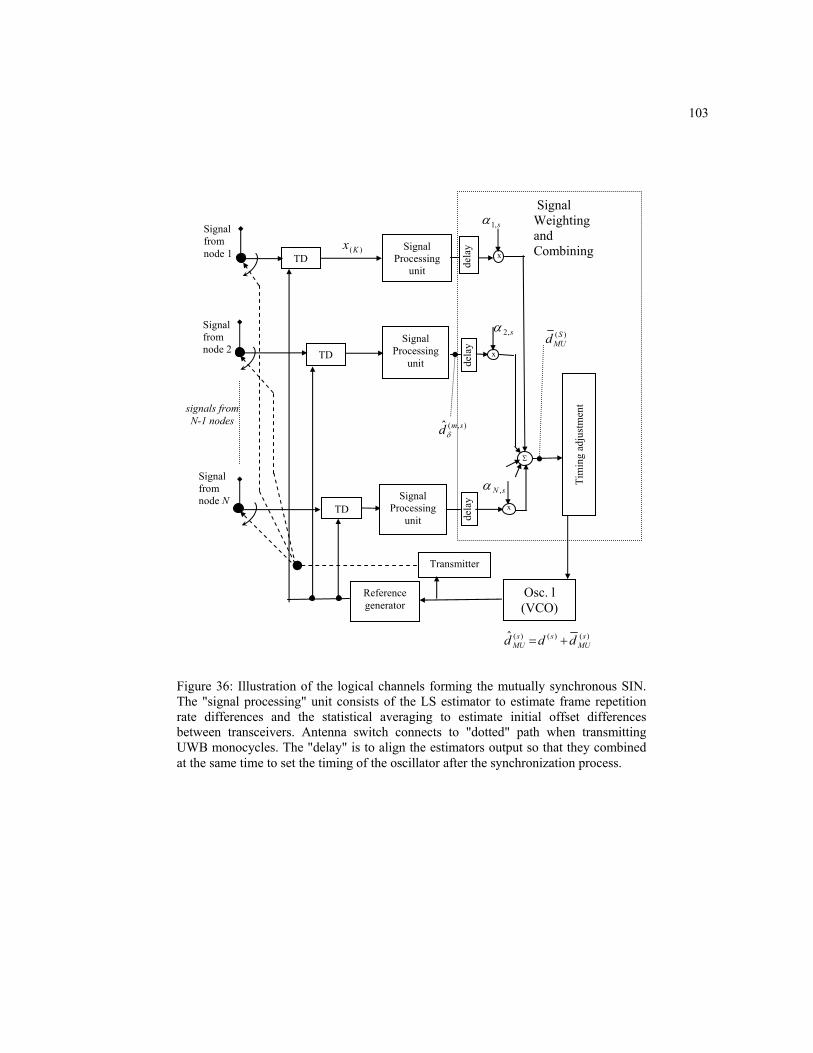
103
Figure 36: Illustration of the logical channels forming the mutually synchronous SIN. The "signal processing" unit consists of the LS estimator to estimate frame repetition rate differences and the statistical averaging to estimate initial offset differences between transceivers. Antenna switch connects to "dotted" path when transmitting UWB monocycles. The "delay" is to align the estimators output so that they combined at the same time to set the timing of the oscillator after the synchronization process.
)(Kx
Signal Processing
unit
Signal Weighting and Combining
s,2α
Signal Processing
unitTD
Signal from node 1
TD
Signal from node 2
Transmitter
Signal from node N
Osc. l (VCO)
signals from N-1 nodes
Σ
sN ,α
TD
Tim
ing
adju
stm
ent
x
x
x
s,1α
Signal Processing
unit
dela
y de
lay
dela
y
Reference generator
),(ˆ smdδ
)(SMUd
)()()(ˆ sMU
ssMU ddd +=
104
CHAPTER V
TIME-TRANSFER ERRORS
From Chapter 1, if )()'(
mkt and )(
)'(skt are the kth zero crossing of the master and slave nodes m
and s respectively, the timing error between nodes m and s after time-transfer at time 't is
)()(
)()(1
)()(
)()(1
)()(
)()(
sk
ssmk
mmsk
mk dtadtatt ′′′′ −−′−++′=− φφ , (5.1)
where fTkt ′=′ denotes the time at the end of time-transfer. It is evident from (5.1) that a longer t ′
will lead to a larger timing error due to mis-match in oscillator drift )( )(1
)(1
sm aa − .
After time synchronization, the differences in oscillator frame repetition rate and initial offset
will both be random variables. This is because time-transfer is performed in the presence of additive
channel noise and oscillator phase noise. We assume nodes are stationary during time-transfer.
5.1 Hierarchical Master-slave Time-Transfer Error
For single-master-to-multiple-slaves (SM) and hierarchical master-slave (HM) time-transfer
architectures, the variance of the timing error after time transfer is given by
2)()()1()1(1
)()(
)1()( 2
~~~ φσ+−′−+′=′s
HMs
HMs
k'HMk dtadtat-t VV , s∀ , 1≠s . (5.2)
where )()'(
~ skHMt is the settled timing estimate at node s after time transfer. From Chapters 2 and 3, the
difference in initial offset, ),( smdδ between two nodes m and s is estimated by taking the sample
mean of ),( smϑ over K frames. From (3.24a), ),(ˆ,
),(),( ~ˆ smdsm
smsm dd ερδδ ++= , where ),(ˆ
smd
ε is the zero
mean estimation error. The difference in frame repetition rate ),( smγ is estimated via LS estimation
from the ToAs of the frame-synchronization pulses, where ),(),(),(ˆ smsmsmLS LSγεγγ += and 0 ),( =sm
LSγεΕ .
105
In Chapter 4, it is defined that M is an ordered set whose elements are the node label of the
roving masters. The elements in the set are arranged according to the order at which node takes turn to
be the roving master. The element of M is denoted as )(qM where 1||,...,0 −= Mq and 1)0( =M is
the lead master node. If node s acquires its timing from roving master 'm where ')( mQ =M , from
section 4.3, the settled initial offset estimate at node s after HM time-transfer is
∑≠
=−
− ++++=Q
sqq
qqqq
dsQsQ
ds
HM dd)(1
)(),1())(),1((
ˆ),()),((
ˆ)1()( ~~~
M
MMMM
MM ρερε , 1≠s , (5.3a)
and the settled drift estimate is
∑≠
=
−++=Q
sqq
fqq
fsQs
HM TTaaLSLS
)(1
))(),1(()),(()1(1
)( //~
M
MMMγγ εε , 1≠s . (5.3b)
The variable Q , besides denoting a particular roving master 'm in M , i.e., ')( mQ =M , equals the
number of hops (time transfers) from the lead master node to the roving master 'm from which slave
s acquires its timing.
(a) Hierarchical Master-Slave Timing Jitter
In Appendix B, it is derived analytically that the timing error variance for HM is given by
( )
)4.5(.2
/2/2
~~~
)(~~
2
)(1
))(),1((ˆ
))(),1(()),((ˆ
)),((
2
)(1
)(),1(),()()1(2)()1(
12)(
)()1()(
ΕΕ
VVΕ
M
MMMMMM
M
MMM
φ
γγ
σ
εεεε
ρρ
+
′⋅⋅⋅+′⋅⋅⋅+
++−+′⋅−=−
∑
∑
≠=
−−
≠=
−′′
Q
sqq
fqq
dqq
fsQ
dsQ
Q
sqq
qqsQs
HMs
HMs
kHMk
TtTt
ddtaatt
LSLS
where ∑−
=−⋅⋅=⋅
1
0
),(),(ˆ
),( ))(()/1(K
kST
smsmd
sm KkKLSLS
θεεε γγ VΕ . For HM time-transfer, fTkt ''= where
||)12(' M⋅⋅−= KNk . In (5.4), when timing is transferred from roving master node )(QM to node s ,

106
the starting index is QKNK ST ⋅⋅−= )12( . For the accumulated timing error variance from one roving
master node ( )1( −qM ) to another ( )(qM ), )1()12( −⋅⋅−= qKNK ST , 1≥q .
For time-transfer scheme A described in section 3.1 where each node transmits in contiguous
frames, the variance of the timing error is
( )
)5.5(.2
/))(),1((2
1)1()12(22122
/)),((2
1)12(22122
~~
~
)(~~
2
)(1
23
23
2
)(1
)(),1(),(
)()1(2)()1(1
2)()(
)1()(
MM
M
VVΕ
M
M
MMM
φσ
σ
σ
ρρ
+
′⋅−⋅
+−⋅⋅−⋅−−⋅⋅+
′⋅⋅
+⋅⋅−⋅−−⋅⋅+
++
−+′⋅−=−
∑
∑
≠=
≠=
−
′′
f
Q
sqq
x
fx
Q
sqq
qqsQ
sHM
sHM
skHMk
TtqqqKNKNK
K
TtsQQKNKNK
K
ddtaatt
It is interesting to note that the coefficient 2/)1)12(22( +−−− KQNKNK of )),((2 sQx Mσ , resulting
from the cross-correlation between drift )~( )()1(1
sHMaa − and initial offset )
~( )()1( s
HMdd − errors, is negative
if )2/()12( KNKKNKQ −+−> . For realistic cases considered in this work, the denominator
KNK −2 is always greater than the numerator 12 +− KNK . Therefore the cross-correlation term is
always negative.
If )()'(
~ skSMt is the settled timing at node s after master-slaves time-transfer, where
KNk )12(' −= , the timing error can be obtained from (5.4) by letting 0=Q , then
( )
)6.5(,2/2
~~
)(~~
2),1(ˆ
),1(
2,1
)()1(2)()1(1
2)()(
)1()(
Ε
VVΕ
φγ σεε
ρ
+′⋅⋅⋅+
+−+′⋅−=− ′′
fs
ds
ss
SMs
SMs
kSMk
Tt
ddtaatt
LS
where ~ )()1(1
sSMaa −V and
~ )()1( s
SMdd −V are given by equations (4.2a) and (4.2b) in Chapter 4.
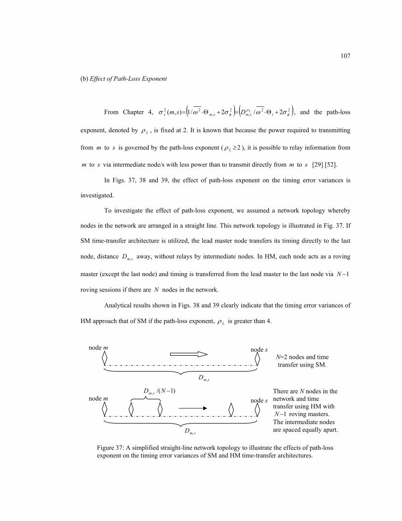
107
(b) Effect of Path-Loss Exponent
From Chapter 4, ( ) ( )22,
2,
22 2/2/1),( φρ
φ σωσωσ +Θ⋅=+Θ⋅= tsmsmxLDsm , and the path-loss
exponent, denoted by Lρ , is fixed at 2. It is known that because the power required to transmitting
from m to s is governed by the path-loss exponent ( 2≥Lρ ), it is possible to relay information from
m to s via intermediate node/s with less power than to transmit directly from m to s [29] [52].
In Figs. 37, 38 and 39, the effect of path-loss exponent on the timing error variances is
investigated.
To investigate the effect of path-loss exponent, we assumed a network topology whereby
nodes in the network are arranged in a straight line. This network topology is illustrated in Fig. 37. If
SM time-transfer architecture is utilized, the lead master node transfers its timing directly to the last
node, distance smD , away, without relays by intermediate nodes. In HM, each node acts as a roving
master (except the last node) and timing is transferred from the lead master to the last node via 1−N
roving sessions if there are N nodes in the network.
Analytical results shown in Figs. 38 and 39 clearly indicate that the timing error variances of
HM approach that of SM if the path-loss exponent, Lρ is greater than 4.
node m node s
smD ,
N=2 nodes and time transfer using SM.
node m node s
smD ,
There are N nodes in the network and time transfer using HM with
1−N roving masters. The intermediate nodes are spaced equally apart.
)1/(, −ND sm
Figure 37: A simplified straight-line network topology to illustrate the effects of path-loss exponent on the timing error variances of SM and HM time-transfer architectures.

108
Figure 38: Normalized timing error standard deviation with path-loss exponent 2=Lρ at 30=Θ t dB, 0=φσ and 1000=K . The network topology is shown in Figure 37. Results
obtained using (a) time- transfer scheme A and (b) time-transfer scheme C.
1.E-02
1.E-01
1.E+00
1.E+01
1.E+02
10 20 30 40 50 60 70 80 90 100
SM architecture
SM,30 dB
HM,N=10,30 dB HM,N=30,30 dBHM,N=20,30 dB
smD , (meters)
Nor
mal
ized
tim
ing
erro
r st
anda
rd d
evia
tion
ws
kH
Mm k
tt
σ/)
(2
)(
)'(
)(
)'(
−Ε
(a) Time-transfer scheme A
1.E-03
1.E-02
1.E-01
1.E+00
10 20 30 40 50 60 70 80 90 100
SM architecture
SM,30 dB
HM,N =10,30 dB HM,N =30,30 dBHM,N =20,30 dB
smD , (meters)
ws
kH
Mm k
tt
σ/)
(2
)(
)'(
)(
)'(−
Ε
Nor
mal
ized
tim
ing
erro
r st
anda
rd d
evia
tion
(b) Time-transfer scheme C
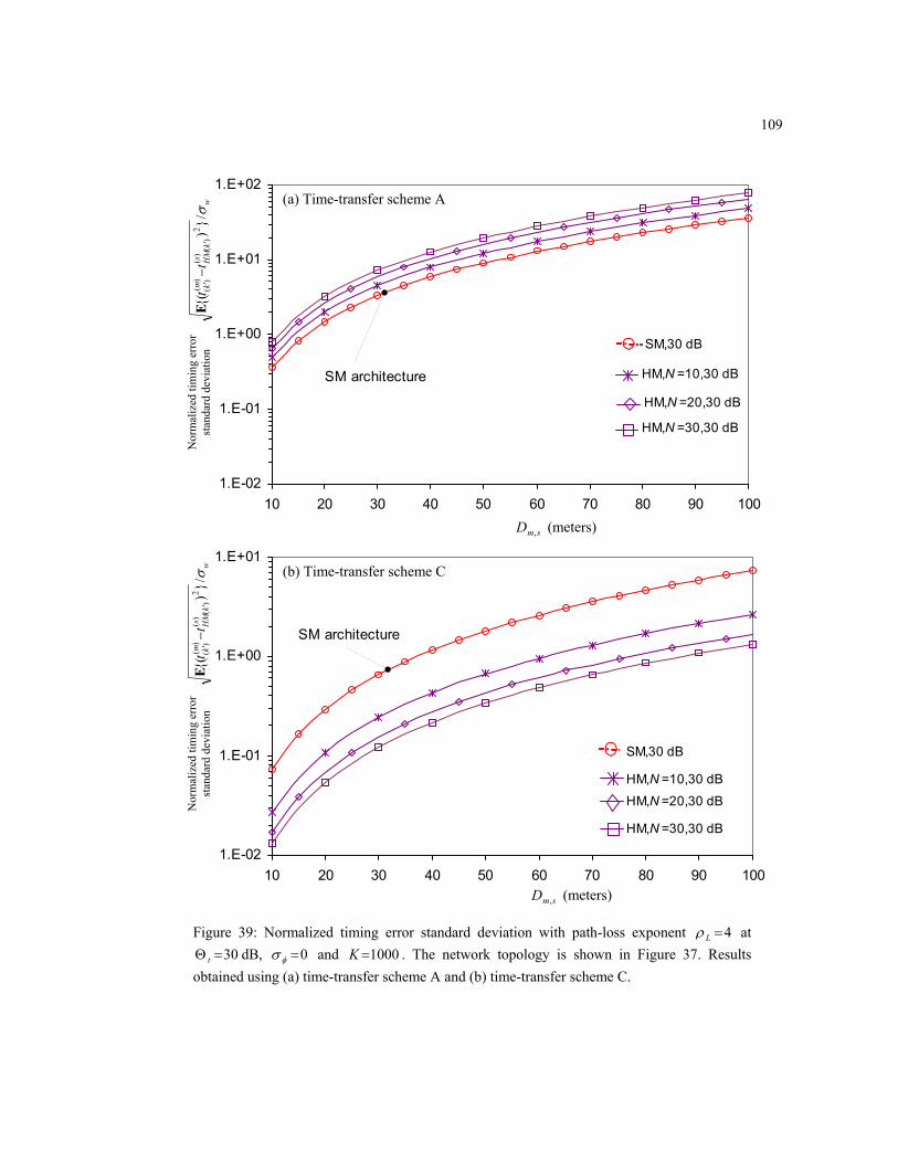
109
1.E-02
1.E-01
1.E+00
1.E+01
1.E+02
10 20 30 40 50 60 70 80 90 100
SM architecture
SM,30 dB
HM,N =10,30 dB
HM,N =30,30 dB
HM,N =20,30 dB
smD , (meters)
ws
kH
Mm k
tt
σ/)
(2
)(
)'(
)(
)'(−
Ε
Nor
mal
ized
tim
ing
erro
r st
anda
rd d
evia
tion
Figure 39: Normalized timing error standard deviation with path-loss exponent 4=Lρ at 30=Θ t dB, 0=φσ and 1000=K . The network topology is shown in Figure 37. Results
obtained using (a) time-transfer scheme A and (b) time-transfer scheme C.
1.E-02
1.E-01
1.E+00
1.E+01
10 20 30 40 50 60 70 80 90 100
SM architecture
SM,30 dB
HM,N =10,30 dB
HM,N =30,30 dB
HM,N =20,30 dB
smD , (meters)
ws
kH
Mm k
tt
σ/)
(2
)(
)'(
)(
)'(−
Ε
Nor
mal
ized
tim
ing
erro
r st
anda
rd d
evia
tion
(a) Time-transfer scheme A
(b) Time-transfer scheme C

110
5.2 Mutually Synchronous Time-Transfer Error
(a) Mutually Synchronous Timing Jitter
Let the settled timing estimate at node s at the end of mutually synchronous time-transfer be
)()'(
)()()()'(
~~~ sk
sMU
sMU
skMU dtat φ++′⋅= , (5.7)
where fTkt ′=′ and NKNk ⋅⋅−= )12(' . The oscillator timing jitter sequence )()'(
skφ is assumed to be
independently identically distributed with zero mean and variance 2φσ . From Appendix B, the
expected value of the squares of (5.7) is
( ) ( ) ( ) ( ) )(~~2
~~~ 2)()'(
)()(2)(22)(2)()'(
sk
sMU
sMU
sMU
sMU
skMU tdadtat φΕΕΕΕΕ +′⋅⋅⋅++′⋅= , (5.8)
where
( ) ( ) ( ) ( ) 22),(21
1
2)1,(2)1(1
2)( //~f
sNf
N
n
nnsMU TTaa
LSLS γγ εε ΕΕΕ ++= ∑−
=
+ , (5.9a)
( ) ( ) ∑∑≠=
≠=
⋅+
+⋅=
N
smm
smdsm
N
smm
smm
sms
MU dd,1
2),(ˆ
2,
2
,1,
)(,
2)( )~(~
εαρα ΕΕ , (5.9b)
and
c)9.5(.
~~
,1
),(ˆ
),(,
1
1 ,1
),(ˆ
)1,(,
,1,,
)1(1
,1
)(,
)1(1
)()(
Ε
ΕΕ
∑
∑ ∑∑∑
≠=
−
=≠=
+
≠=
≠=
⋅⋅+
⋅⋅+⋅+⋅=⋅
N
smm
smd
sN
f
sm
N
n
N
smm
smd
nn
f
smN
smm
smsm
N
smm
msm
sMU
sMU
LS
LS
T
Tadada
εεα
εεα
ραα
γ
γ
The sample variance of )()'(
~ skMUt is defined to be
∑ ∑= =
−
−
N
s
N
s
skMU
skMU t
Nt
N 1
2
1
)()'(
)()'(
~1~1
1 . (5.10)

111
For a MU time-transfer architecture, unlike HM, there is no "preferred" node in the network.
To characterize the performance of the MU time-transfer architecture, we consider the timing
variances across all nodes in the network. One appropriate measure is the mean of the sample variance
of )()'(
~ skMUt , s∀ , at time fTkt ′=′ where NKNk ⋅⋅−= )12(' . The mean of the timing variances across all
nodes in the network is defined as
−
−= ∑∑
==
2
1
)()'(
1
2)()'()'(
~1)~(1
1~N
s
skMU
N
s
skMUkMU t
Nt
Nt ΕV . (5.11)
In Appendix B, it is shown that
21
1
),(ˆ
),(,2)'( 2
~)(~~ φγ σεε
α+⋅⋅
′⋅++′⋅= ∑
−
=
N
s
sNd
sN
f
sNMUMUkMU LSTN
tdtat ΕVVV , (5.12)
where ∑−
=−⋅⋅=⋅
1
0
),(),(ˆ
),( ))(()/1(K
kST
smsmd
sm KkKLSLS
θεεε γγ VΕ and )1()12( −⋅⋅−= NKNK ST . The mean of
the sample variances of the settled drift and initial offset estimates for all nodes in the network are
derived earlier in Chapter 4, and they are
∑=
⋅=N
sf
N,sγMU Tε
Na
LS1
)( /1~ VV ,
( ) ( )2
1 .1,
)(,
1 1
2
.1,
)(,
)( ~)1(
1~1
1~
1~
+⋅
−⋅−
+⋅
−+= ∑ ∑∑ ∑ ∑
= ≠== = ≠=
N
s
N
smmsm
msm
N
s
N
s
N
smmsm
msm
sMUMU d
NNd
Nd
Nd ραραVV .
(b) Effect of Different Weight Functions
In Fig. 40, the sample timing variances ~ )'(kMUtV obtained via (5.12) for a particular
network topology (shown in Fig. 42 of Chapter 6) with 20=N at various SNR is presented. The plots
in the figure are the timing variances when different weight functions sm,α are substituted into (5.12).
For this particular example, the differences in timing variances obtained using the three different
weight functions are not significant.
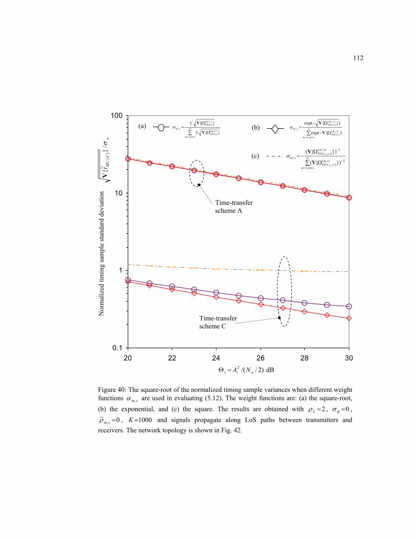
112
0.1
1
10
100
20 22 24 26 28 30
Figure 40: The square-root of the normalized timing sample variances when different weight functions sm,α are used in evaluating (5.12). The weight functions are: (a) the square-root, (b) the exponential, and (c) the square. The results are obtained with 2=Lρ , 0=φσ ,
0~, =smρ , 1000=K and signals propagate along LoS paths between transmitters and
receivers. The network topology is shown in Fig. 42.
)2//(2ott NA=Θ dB
w
kM
Ut
σ/~
')(
V
(a) (b)
(c)
Nor
mal
ized
tim
ing
sam
ple
stan
dard
dev
iatio
n
∑≠=
Ω
Ω= N
smm
smzDN
smzDN
sm
,1
),()(
),'()(
,'
/1
1
V
Vα
∑≠=
Ω−
Ω−= N
smm
smzDN
smzDN
sm
,1
),()(
),'()(
,'
)exp(
)exp(
V
Vα
∑≠=
−
−
Ω
Ω= N
smm
smijzDN
smijzDN
sm
,1
2),(),,(
2),'(),,(
,'
)(
)(
V
Vα
Time-transfer scheme C
Time-transfer scheme A

113
5.3 Summary of Time-Transfer Equations
For ease of reference, the variances in estimating the differences in frame repetition rate,
initial offset and timing errors using the SM, HM and MU time-transfer architectures presented in
earlier chapters are tabulated in Tables 2, 3 and 4. The zero mean error of the initial-offset equation is
given by
4),(),(5
22
),( mssm xxsm σσεϑ
+⋅=V .
The cross-correlation between the LS estimation error and initial offset estimation error is
∑−
=−⋅⋅=⋅
1
0
),(),(ˆ
),( ))((1K
kST
smsmd
sm KkK LSLS
θεεε γγ VΕ .
The variance of the initial offset estimation error between nodes m and s is
))((
),(),(2
21
0),( smsm
K
kST
smLSK
Kkd ϑγδ εε
θVVV +⋅
−
=∑−
= .
The variance of uplink ToAs is
),()(
2),(),()(
msuUP
smmsuUP u
LSεε γ VVV +⋅=Ω .
The variance of downlink ToAs is
)( ),()(
2),(),()(
smzDN
smmszDN uz
LSεε γ VVV +−⋅=Ω .
The variance of the measurement error when measuring uplink ToAs is
),(),(2 222),()( msms xn
msuUP σσσε φ =+⋅=V .
The variance of the measurement error when measuring downlink ToAs is
),(),( 22),()( smms xx
smuDN σσε +=V .
The variance of the output of the open-loop timing detector is 222,
2 2)/(),( φσωσ +Θ⋅= tsmx Dsm .

114
Table 2: Equations that defined the various time-transfer schemes
kKNk −
−=
2)1()(θ , 1,...,1,0 −∈ Kk
STKkv += , kKKjKu ST ++⋅−+= )2( and KNuz ⋅−=− )1( .
3
2),( ),(12
Ksmxsm
LS
σε γ
⋅=V
)3212()12(
)1(),(3
ˆ ),(2
22
),( smSTSTxsm
KKNKKKK
NK
smd ϑδ ε
σVV +
+−−⋅−++−⋅
⋅=
−
+−⋅⋅=⋅ STx
smd
sm KKNKsmKLS 2
12),(12 23
),(ˆ
),( σεε γΕ
kNNk ⋅−−
−= )12(
21)(θ , 1,...,1,0 −∈ Kk
STKkNv +⋅−= )12( , STKkNju +⋅−+−+= )12()2(1 and 1−=− Nuz .
23
2),(
)12(1),(12
−
⋅⋅
=NK
smxsmLS
σε γV
( ) )1()12(12)12(),(3
ˆ ),(223
2),( sm
STxsm KNKN
NKsm
d ϑδ εσ
VV +−⋅−−−−⋅−⋅
⋅=
−−⋅−−−
⋅−⋅
⋅=⋅ ST
xsmd
sm KKNN
NKsm
LS 2)1()12(1
)12(),(12
23
2),(
ˆ),( σεε γΕ
kNk ⋅−−= )12(
21)(θ , 1,...,1,0 −∈ Kk
STKkNv +⋅−= )12( , STKkNju +⋅−+⋅−+= )12(2)2(1 and 1=−uz .
23
2),(
)12(1),(12
−
⋅⋅
=NK
smxsmLS
σε γV
( ) 222)12(),(3
ˆ ),(223
2),( sm
STxsm KNKKN
NKsm
d ϑδ εσ
VV +−−+⋅−⋅
⋅=
−−⋅−−
⋅−⋅
⋅=⋅ ST
xsmd
sm KKN
NKsm
LS 2)1()12(1
)12(),(12
23
2),(
ˆ),( σεε γΕ
Tim
e-tra
nsfe
r sch
eme
A
Tim
e-tra
nsfe
r sch
eme
B
Tim
e-tra
nsfe
r sch
eme
C

115
Table 3: Variances of the estimation error in estimating the differences in frame repetition rate and initial offset for SM, HM and MU time-transfer architectures
2),1()()1(1 /~ f
ssSM Taa
LSγεVV ≥− , ,...,2 Ns∈ . SM
2,1
),1(),1(2)()1( ~ˆ)~
( ssss
SM ddd ρεϑδ ++=− VVΕ , 0=STK .
=
>⋅+=−
∑≠
=
−
.0,/
.0,/~
2),1(
2
)(1
))(),1((2),1(
)()1(1
QT
QTTaa
fs
f
Q
sqq
qqf
s
sHM
LS
LSLS
γ
γγ
ε
εε
V
VVV M
MM
HM
2
)(,1
)(),1(),()()1(2)()1( ~~)
~()
~(
++−=− ∑
≠=
−
Q
sqq
qqsQs
SMs
SM ddddM
MMMVΕ ρρ , where
=+=
>+++=
−
∑≠
=
−−
.0,ˆ
.0,ˆˆ
~
),1(),1()(1
))(),1(())(),1(()),(()),((
)()1(
Qd
Qdd
dd
ss
Q
sqq
qqqqsQsQ
sHM
ϑδ
ϑδϑδ
ε
εε
VV
VVVV
V
Μ
MMMMMM
If 0=Q , 0=STK .
If 0>Q , in ˆ )),(( sQd MV δ , QKNKST ⋅⋅−= )12( .
In ˆ ))(),1(( qqd MMV −δ , )1()12( −⋅⋅−= qKNKST , 1≥q .
.//~ 2)(1
1
2)1()(f
N,sγ
N-
nf
n,nγ
sMU TεTεa
LSLSVVV +=∑
=
+
MU 2
,1,
)(,
,1
),(2,
2)( )~(ˆ)~
(
+⋅+⋅= ∑∑
≠=≠=
N
smmsm
msm
N
smm
smsm
sMU ddd ραα δVΕ .
Assuming ,...,2,1 N∈M , STK in ˆ ),( smdδV is given by )1()12( −⋅⋅−= mKNKST .

116
Table 4: Variances of timing error for SM, HM and MU time-transfer architectures
SM
( ) ,2/2
~~
)(~~
2),1(ˆ
),1(
2,1
)()1(2)()1(1
2)()(
)1()(
φγ σεε
ρ
+′⋅⋅⋅+
+−+′⋅−=− ′′
fs
ds
ss
SMs
SMs
kSMk
Tt
ddtaatt
LSΕ
VVΕ
where fTKNt ⋅⋅−= )12(' , 0=STK .
HM
( )
.2
/2
/2
~~~
)(~~
2
)(1
))(),1((ˆ
))(),1((
)),((ˆ
)),((
2
)(1
)(),1(),()()1(2)()1(
12)(
)()1()(
φ
γ
γ
σ
εε
εε
ρρ
+
′⋅⋅⋅+
′⋅⋅⋅+
++−+′⋅−=−
∑
∑
≠=
−−
≠=
−′′
f
Q
sqq
qqd
fsQ
dsQ
Q
sqq
qqsQs
HMs
HMs
kHMk
Tt
Tt
ddtaatt
LS
LS
M
MMMM
MM
M
MMM
Ε
Ε
VVΕ
Here ||)12(' M⋅⋅⋅−= fTKNt . Values of STK are given in Table 3.
MU
21
1
),(ˆ
),(,2)'( 2
~)(~~ φγ σεε
α+⋅⋅
′⋅++′⋅= ∑
−
=
N
s
sNd
sN
f
sNMUMUkMU LSTN
tdtat ΕVVV ,
where NTKNt f ⋅⋅⋅−= )12(' ,
∑−
=⋅
⋅=
1
1
2),(2 )(1~
N
s
sN
fMU LSTN
a γεΕV , and
( )
( ) .~)1(
1
~1
1~
1~
2
1 .1,
)(,
1 1
2
.1,
)(,
)(
+⋅
−⋅−
+⋅
−+=
∑ ∑
∑ ∑ ∑
= ≠=
= = ≠=
N
s
N
smmsm
msm
N
s
N
s
N
smmsm
msm
sMUMU
dNN
dN
dN
d
ρα
ραVV
Values of STK are given in Table 3.
Note that )(kθ is the characteristic function of the time-transfer scheme and STK is the starting index
of the ToA measurements to be used to estimate the initial offset differences. In Fig. 41, the
normalized timing error variance computed from Table 4 for a SM time-transfer architecture with a
circular network topology is shown.

117
Figure 41: Timing error variance for a circular network topology synchronized with SM. The performance of different time-transfer schemes is first described in sections 3.1 and 3.4. In this plot, =Θ sm, 20 dB, 0=STK , 0=φσ and 0~
, =smρ .
1.E-03
1.E-02
1.E-01
1.E+00
1.E+01
1.E+02
1.E+03
1.E+04
0 20 40 60 80 100
K=1
K=10
K=100
K=1000
N, number of nodes in the network
Time-Transfer Scheme A
Time-Transfer Scheme B
Time-Transfer Scheme C
Nor
mal
ized
stan
dard
dev
iatio
n of
tim
ing
erro
r
12−Nπ
Network topology
(1) (s)
w
sk
SMk
tt
σ/~
)
()'
()1()'
(−
V

118
There exist other possibilities to arrange the frame-synchronization, uplink and downlink
pulses. For example, the downlink pulse can be "returned" to the slave in the same frame as the uplink
pulse arrives at the master node, that is, the master node acts like a relay to complete the two-way
ranging (this is similar to that performed in the RTS). In this case, uz= and the total number of
uplink plus downlink frames is reduced by half. Although the time needed for synchronization has
now reduced approximately by half, it does not bring about a lower timing jitter for schemes B and C.
This is because the variance of estimating the frame-repetition rate difference is now increased by a
factor of 2 as the spacing between the frame-synchronization pulses is reduced by half. Further, it can
be shown that the characteristic function of this scheme will be kNk ⋅−−= )12()(θ and if 1>>K ,
ˆ ),( smdδV for this scheme will be similar to that of time-transfer scheme C. However, by making
uz= , the timing jitter after time transfer using time-transfer scheme A will be smaller due to a
shortening of the time needed to perform synchronization while the spacing between the frame-
synchronization pulses remains at fT .

119
CHAPTER VI
SIMULATIONS AND OBSERVATIONS
The earlier chapters have presented the theoretical formulations of the proposed time transfer
schemes (time-transfer schemes A, B and C) and described the various time-transfer architectures to
implement a SIN. This Chapter presents the computer simulations results. It is followed by a
discussion of the advantages and disadvantages of the single-master-to-multiple-slaves (SM),
hierarchical master-slaves (HM) and mutually synchronous time-transfer (MU) architectures.
When SM and HM are used to perform time synchronization, the timing jitter is defined as
the variance of the timing error between the lead master node (node 1) and other nodes in the network.
For MU time-transfer architecture, the sample variance of the timings of all nodes in the network is
defined to be the timing jitter.
6.1 Simulation of Proposed Time-Transfer Architectures
To verify the theoretical formulations presented in earlier chapters and to gain further insight
into the working of the proposed SIN, the various time transfer architectures, namely, the SM, HM
and the MU time-transfer architectures are simulated.
The simulations assume that the received SNR is sufficient for the AGC described in Chapter
2 to be effective in controlling the amplitude of the received UWB monocycles and for the timing
detector to operate at the linear region of its characteristic function. Therefore equations (3.1), (3.3a)
and (3.4b), which describe the measured ToAs, are simulated. The measured ToAs are impaired by
additive channel noise, the oscillator's phase noise and network NLoS signal propagations. The
additive noise samples are drawn from a Gaussian distribution with zero mean and variance ),(2 smnσ .

120
The oscillator phase noise samples have a uniform probability density function with zero mean and
variance 2φσ . Each simulation result is obtained with at least 500 Monte Carlo steps.
The simulations implemented the techniques described in Chapter 3 to estimate the
differences in fame repetition rate and initial offset between network nodes. The various time-transfer
architectures described in Chapter 4 are also implemented accordingly.
The simulations first performed on a given network topology. With a given network
topology, the timing variances at each network node are observed. This is follows by allowing the
network nodes to be randomly distributed over a given area and the ensemble averages of the timing
variances are observed.
6.1.1 Simulations with a given Network Topology
A SIN is simulated for a given network topology shown in Fig. 42 with 20=N . In the
simulations, time synchronization is performed using the SM, HM and MU time-transfer
architectures. The simulation parameters are (unless otherwise specified): 1000=== rs KKK frames,
0=φσ sec, effective squared bandwidth =2ω 1.9×10²¹ sec-2, initial offset of network nodes before
time transfer are ∈)(sd -0.15, 0.10, 0.17, 0.07,-0.07,-0.02, 0.05, 0.25, 0.23, 0.09, 0.11, 0.10, 0.28,
0.01, 0.10, 0.12, 0.003, 0.071, 0.271, 0.14 ×10⁻⁹ sec. And drift of network nodes before time transfer
are η+=1)(sa where ∈η 0, 7,-4, 9, 5, 4,-8,-5, 2,-7, 8, 1, 7,-4, 8, 5, 7, 4, 3,-2×10⁻⁶.
It is discussed in section 2.3.4 that when the scattering environment changes, the uplink and
downlink excess-delay may not be equal, as a result, 0~, ≠smρ . This is more likely for time-transfer
scheme A because nodes transmit the uplink and downlink ranging pulses in time slots that are
temporally far apart if number of network nodes is large. In time-transfer scheme C, the uplink and
downlink pulses are transmitted in adjacent frames and hence it is least likely that the scattering

121
environment changes in between transmissions. Further, sm,~ρ is also used to model any receiver
processing errors that may arise when the timing detector lock onto a NLoS path.
In this work, it is assumed that sm,~ρ is not random. It will be left to future research to model
sm,~ρ as a random variable.
To illustrate the effects of sm,~ρ (to be summarized as receiver processing error), links
between selected nodes are replaced with a longer propagation path. The selected links are:
cD ⋅+= )( 15,115,115,1 ρτ , cD ⋅+= )( 17,117,117,1 ρτ and cD ⋅+= )( 20,120,120,1 ρτ where c is the speed of light.
The excess-delays due to NLoS propagation are: 15,115,1 5.0 τρ ⋅= , 17,117,1 5.0 τρ ⋅= and 20,120,1 5.0 τρ ⋅= .
As a result, the receiver measurement errors are: 15,115,1 25.0~ τρ = , 17,117,1 25.0~ τρ = and 20,120,1 25.0~ τρ = .
The HM network described in section 4.3 is simulated with the network topology shown in
Fig. 42. In Figs. 43 to 45, the normalized standard deviation of the estimated differences in initial
offset between the lead master and selected nodes 2, 17 and 9 at 20=Θ t dB to 30 dB are shown.
Node 9 is the furthest node in the network from the lead master. Node 2 is about half-way between
lead master and node 9. The transmitted signal propagates from node 1 to node 17 via a NLoS path
with 17,117,1 25.0~ τρ = . In Figs. 46 to 48, the timing error variances )~( 2)()'(
)1()'(
skHMk tt −Ε for nodes 2, 17
and 9 are plotted. For HM with five roving masters, 5)12(' ⋅−= fKTNt , while nineteen roving masters
require a synchronization time of 19)12(' ⋅−= fKTNt to synchronize 20=N nodes in the network.
The results shown in Figs. 43 and 48 are obtained using time-transfer scheme A.
Not illustrated in Figs. 43 to 48 is the fact that during simulations when oscillator jitter 2φσ is
significant compared to jitter due to channel noise, there is increased randomness in the selection of
nodes to be the next roving masters. For example, if 0=φσ , using only 5 roving masters, the order of
the roving master is 1,8,12,4,2 in almost all simulation runs, which corresponds to the shortest
propagation distances between nodes. In this case, simulation results agree well with the results
122
obtained from theoretical formulations (the equations of the timing variances are listed in Tables 3
and 4). At 1110−=φσ secs, order of roving master can be as different as 1,8,12,7,4 or 1,4,7,2,12
and some other possibilities at various SNR. This causes an increase in timing jitter in some nodes
because time-transfer is no longer via the shortest possible hops for these nodes. Similar observations
are made when all nodes in the network (except the last node) take turns being the roving master.
The MU network described in section 4.4 is simulated for 20=N with nodes distributed as
shown in Fig. 42. The quantity ( ) 2)(~ sMUdΕ is plotted in Fig. 49 at 30=Θ t dB for 0=φσ . The mean of
the timing sample variance of all nodes in the network after MU architecture (utilizing time-transfer
scheme A) is indicated as a horizontal line in Fig. 50. In Fig. 51, the timing sample variance ~ MUtV
is plotted when time-transfer between pair of nodes is performed using time-transfer scheme C. The
simulation results agree well with the theoretical formulations.
Included in Figs. 49 to 51 are also estimation variances when HM and SM time-transfer
architectures are utilized to perform time synchronization at 30=Θ t dB. The timing error variances
after time transfer with HM and SM are plotted in the same figure together with the network timings
sample variance after using MU time-transfer architecture.
It is interesting to note from Fig. 49 and 50 that, for node 8, which is the closest to the lead
master, SM and HM produce the same estimation variance for estimating the initial offset difference
wHMdd σ)~
( 2)8()1( −Ε . However, the corresponding timing error variance at node 8 given by
wkHMk tt σ)~( 2)8()'(
)1()'( −Ε and shown in Fig. 50, no longer coincides. In fact, HM with 19 roving
masters has higher timing error variance than HM with 5 roving masters and SM has the lowest
variance. This is because the time required to perform time synchronization for HM with 19 roving
masters is the longest follows by utilizing 5 roving masters. The longer synchronization time
multiplied by drift estimation error leads to higher timing error variances.

123
In Fig. 52, the timing sample variances for MU time-transfer are plotted for 0=φσ ,
1110−=φσ sec and the monocycle pulse width is approximately 067.0=wσ nsec.
The variances ~
MUdV and ~ )'(kMUtV will hit a noise floor if the MU synchronization
process is applied repeatedly. This is because ~
)(sMUdV is a function of network topology via smD , ,
noise density oN , φσ , and network parameters N , K . If MU is applied repeatedly, there is a
threshold beyond which the reduction effect of the weight sm,α will not be able to reduce the
variances further. Also, if MU is applied repeatedly, the variances ~ MUaV will increase due to noise
accumulation. The results of repeatedly applying the MU time-transfer architecture with the network
topology shown in Fig. 42 are plotted in Fig. 53. In this simulation, time-transfer scheme C is utilized.
Moreover, to illustrate the effect of repeatedly applying MU, the initial offset before time transfer is
10 times of that used to obtain Figs. 43 to 52.
In estimating the difference in initial offset, the SM architecture achieves the lowest
estimation error variance at a given SNR. However it is not capable of mitigating receiver
measurement error. The HM architecture has the second lowest estimation error variance and selects
propagation paths so as to avoid NLoS measurement. The MU has the highest sample variance after
the estimation process. Its strength is its ability to average out the effect of receiver measurement
error. The same observations apply to the timing error variances.
The simulation results illustrated the robustness of the MU and HM time-transfer
architectures against NLoS measurement error. It is also evident that the topology of a network has a
strong influence on individual node's timing jitter.
More simulation results are included in Appendix C, D, E and F.
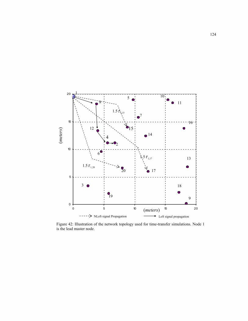
124
1.5 15,1τ
1.5 20,1τ
0
5
10
15
20
0 5 10 15 20
1
2
3
4
5
6
7
8
9
10 11
12
13
1415
16
17
18
19
20
(met
ers)
1.5 17,1τ
(meters)
Figure 42: Illustration of the network topology used for time-transfer simulations. Node 1 is the lead master node.
NLoS signal Propagation LoS signal propagation
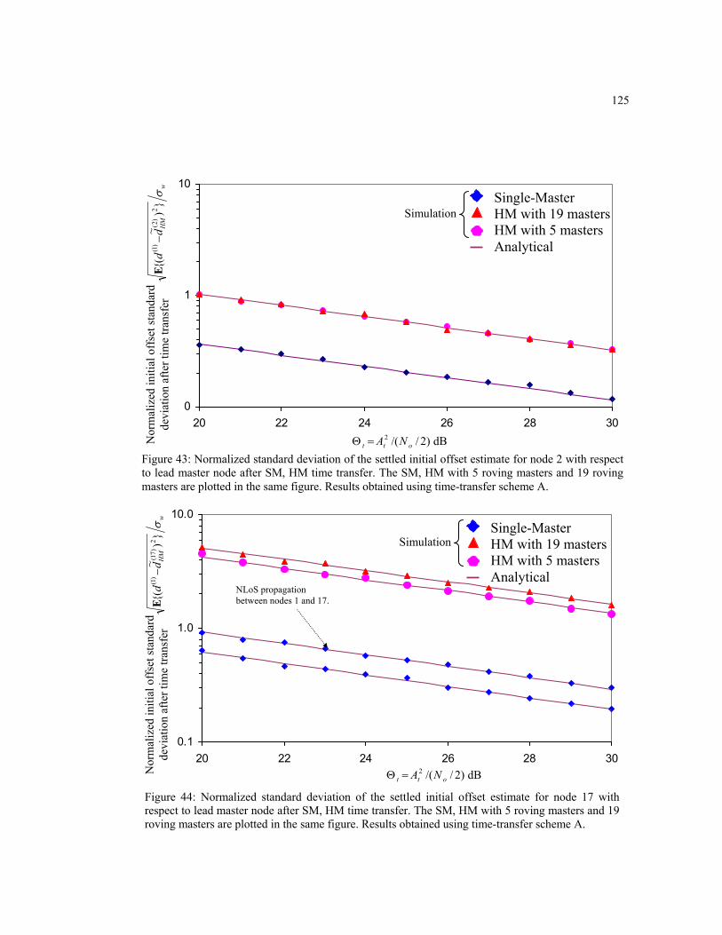
125
0
1
10
20 22 24 26 28 30)2//(2
ott NA=Θ dB Figure 43: Normalized standard deviation of the settled initial offset estimate for node 2 with respect to lead master node after SM, HM time transfer. The SM, HM with 5 roving masters and 19 roving masters are plotted in the same figure. Results obtained using time-transfer scheme A.
Nor
mal
ized
initi
al o
ffse
t sta
ndar
d de
viat
ion
afte
r tim
e tra
nsfe
r
Single-Master HM with 19 masters HM with 5 masters Analytical
Simulation
w
HM
dd
σ
)~
(2
)2()1(−
Ε
0.1
1.0
10.0
20 22 24 26 28 30)2//(2
ott NA=Θ dB
Figure 44: Normalized standard deviation of the settled initial offset estimate for node 17 with respect to lead master node after SM, HM time transfer. The SM, HM with 5 roving masters and 19 roving masters are plotted in the same figure. Results obtained using time-transfer scheme A.
NLoS propagation between nodes 1 and 17.
Nor
mal
ized
initi
al o
ffse
t sta
ndar
d de
viat
ion
afte
r tim
e tra
nsfe
r
Single-Master HM with 19 masters HM with 5 masters Analytical
Simulation
w
HM
dd
σ
)~
(2
)17(
)1(−
Ε
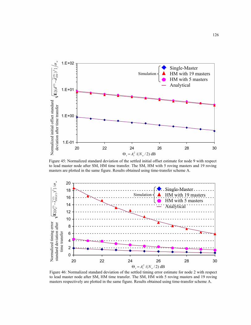
126
0
2
4
6
8
10
12
14
16
18
20
20 22 24 26 28 30
Figure 45: Normalized standard deviation of the settled initial offset estimate for node 9 with respect to lead master node after SM, HM time transfer. The SM, HM with 5 roving masters and 19 roving masters are plotted in the same figure. Results obtained using time-transfer scheme A.
Nor
mal
ized
initi
al o
ffse
t sta
ndar
d de
viat
ion
afte
r tim
e tra
nsfe
r
1.E-01
1.E+00
1.E+01
1.E+02
20 22 24 26 28 30)2//(2
ott NA=Θ dB
Single-Master HM with 19 masters HM with 5 masters Analytical
Simulation
w
HM
dd
σ
)~
(2
)9()1(−
Ε
Figure 46: Normalized standard deviation of the settled timing error estimate for node 2 with respect to lead master node after SM, HM time transfer. The SM, HM with 5 roving masters and 19 roving masters respectively are plotted in the same figure. Results obtained using time-transfer scheme A.
)2//(2ott NA=Θ dB
w
kH
Mk
tt
σ/)
~(
2)2(
')(
)1( '−
Ε
Single-Master HM with 19 masters HM with 5 masters Analytical
Nor
mal
ized
tim
ing
erro
r st
anda
rd d
evia
tion
afte
r tim
e tra
nsfe
r
Simulation
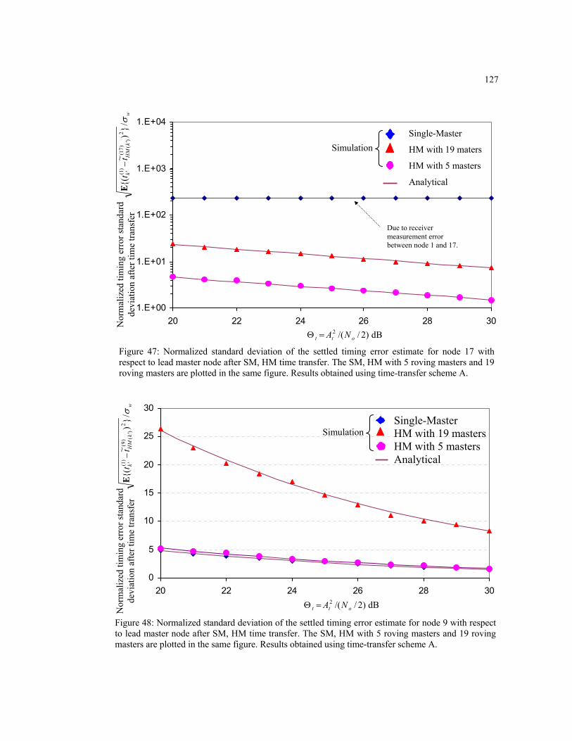
127
Figure 48: Normalized standard deviation of the settled timing error estimate for node 9 with respect to lead master node after SM, HM time transfer. The SM, HM with 5 roving masters and 19 roving masters are plotted in the same figure. Results obtained using time-transfer scheme A.
0
5
10
15
20
25
30
20 22 24 26 28 30)2//(2
ott NA=Θ dB
w
kH
Mk
tt
σ/)
~(
2)9(
')(
)1( '−
Ε
Single-Master HM with 19 masters HM with 5 masters Analytical
Nor
mal
ized
tim
ing
erro
r sta
ndar
d de
viat
ion
afte
r tim
e tra
nsfe
r
Simulation
Figure 47: Normalized standard deviation of the settled timing error estimate for node 17 with respect to lead master node after SM, HM time transfer. The SM, HM with 5 roving masters and 19 roving masters are plotted in the same figure. Results obtained using time-transfer scheme A.
1.E+00
1.E+01
1.E+02
1.E+03
1.E+04
20 22 24 26 28 30)2//(2
ott NA=Θ dB
Due to receiver measurement error between node 1 and 17.
w
kH
Mk
tt
σ/)
~(
2)
17(')
()1( '−
Ε
Single-Master
HM with 19 maters
HM with 5 masters
Analytical
Nor
mal
ized
tim
ing
erro
r sta
ndar
d de
viat
ion
afte
r tim
e tra
nsfe
r
Simulation
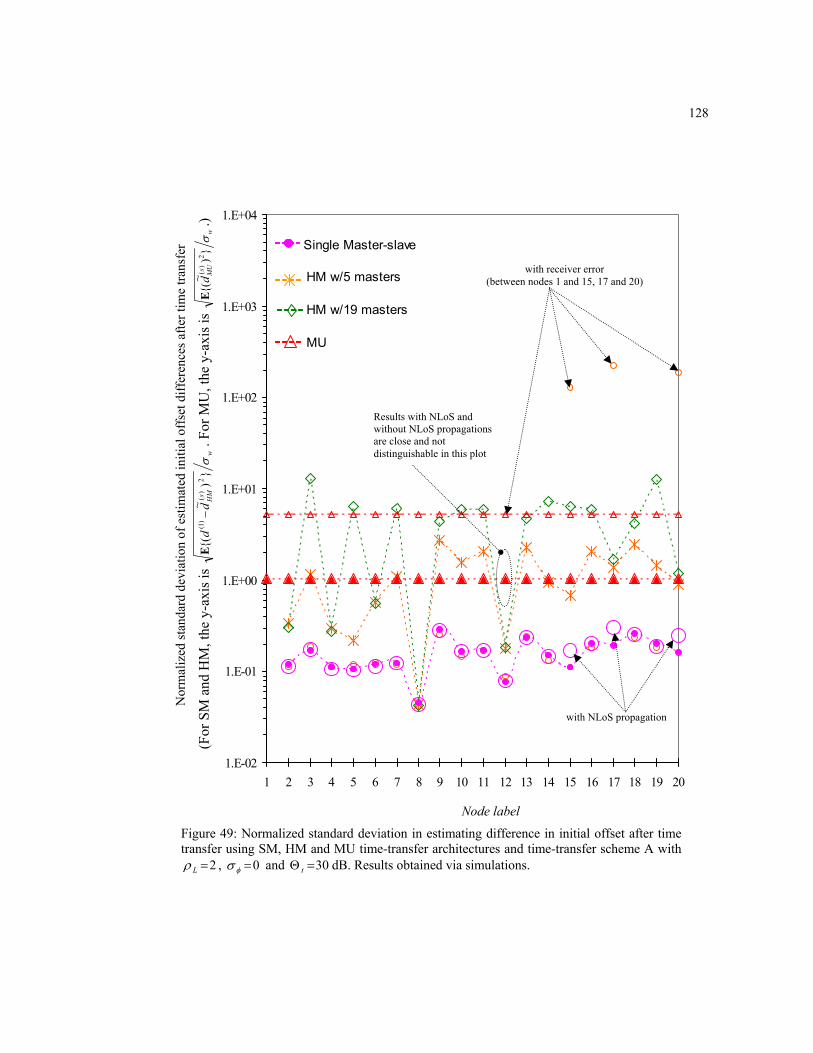
128
1.E-02
1.E-01
1.E+00
1.E+01
1.E+02
1.E+03
1.E+04
1 2 3 4 5 6 7 8 9 10 11 12 13 14 15 16 17 18 19 20
Single Master-slave
HM w/5 masters
HM w/19 masters
MU
Figure 49: Normalized standard deviation in estimating difference in initial offset after time transfer using SM, HM and MU time-transfer architectures and time-transfer scheme A with
2=Lρ , 0=φσ and 30=Θ t dB. Results obtained via simulations.
Nor
mal
ized
stan
dard
dev
iatio
n of
est
imat
ed in
itial
off
set d
iffer
ence
s afte
r tim
e tra
nsfe
r
Node label
with NLoS propagation
with receiver error (between nodes 1 and 15, 17 and 20)
Results with NLoS and without NLoS propagations are close and not distinguishable in this plot
(F
or S
M a
nd H
M, t
he y
-axi
s is
ws HM
dd
σ
)~
(2
)(
)1(−
Ε. F
or M
U, t
he y
-axi
s is
ws
MU
dσ
)
~(
2)
(Ε
.)

129
1.E-01
1.E+00
1.E+01
1.E+02
1.E+03
1.E+04
1 2 3 4 5 6 7 8 9 10 11 12 13 14 15 16 17 18 19 20
Single Master-slave
MU
HM w/5 masters
HM w/19 masters
Figure 50: Normalized standard deviation of timing error after time synchronization using SM, HM and MU time-transfer architectures and time-transfer scheme A with 2=Lρ , 0=φσ and 30=Θ t dB. Results obtained via simulations.
Nor
mal
ized
tim
ing
erro
r/tim
ing
stan
dard
dev
iatio
n af
ter t
ime
trans
fer
Node label
(F
or S
M a
nd H
M, t
he y
-axi
s is
w
sk
HM
kt
tσ
)
~(
2)
()'
()1()'
(−
Ε. F
or M
U, t
he y
-axi
s is
w
kM
Ut
σ
~ )'
(V
.)
Nodes 15, 17 and 20 with NLoS propagation
Nodes 15, 17 and 20 with receiver error
The uppermost trace corresponds to MU with receiver error, middle trace MU with NLoS and lowest trace MU with no NLoS propagation
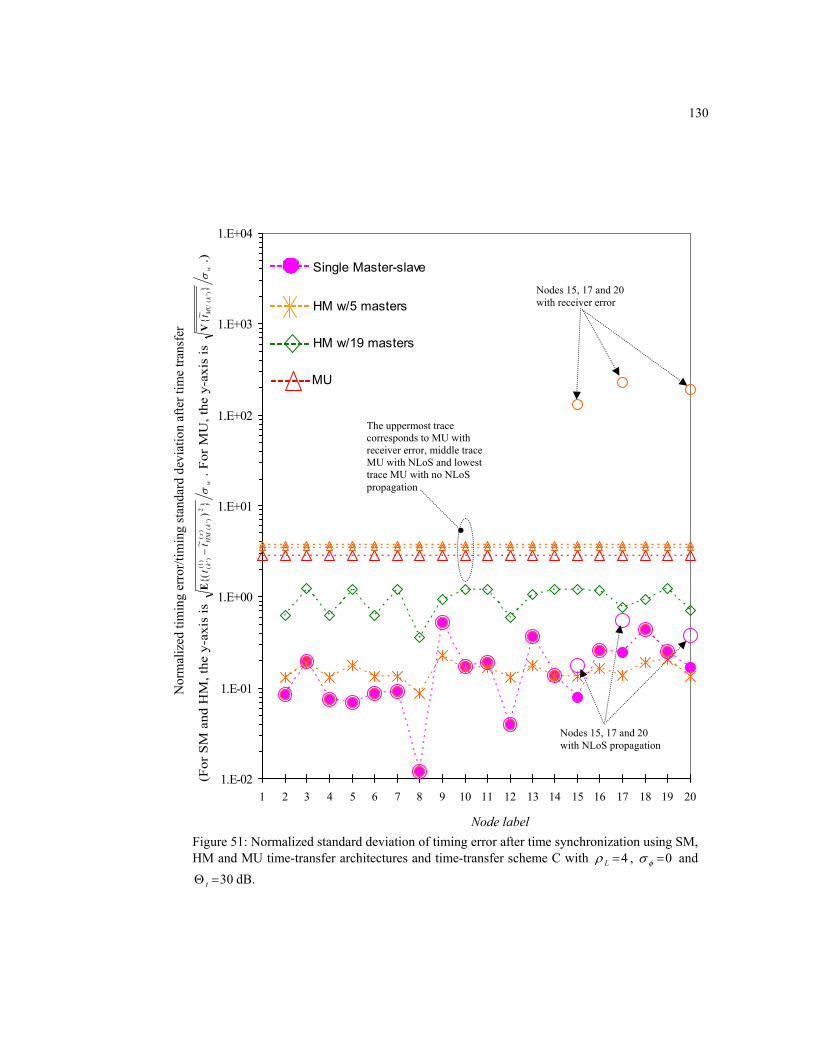
130
1.E-02
1.E-01
1.E+00
1.E+01
1.E+02
1.E+03
1.E+04
1 2 3 4 5 6 7 8 9 10 11 12 13 14 15 16 17 18 19 20
Single Master-slave
MU
HM w/5 masters
HM w/19 masters
Figure 51: Normalized standard deviation of timing error after time synchronization using SM, HM and MU time-transfer architectures and time-transfer scheme C with 4=Lρ , 0=φσ and
30=Θ t dB.
Nor
mal
ized
tim
ing
erro
r/tim
ing
stan
dard
dev
iatio
n af
ter t
ime
trans
fer
Node label
(F
or S
M a
nd H
M, t
he y
-axi
s is
w
sk
HM
kt
tσ
)
~(
2)
()'
()1()'
(−
Ε. F
or M
U, t
he y
-axi
s is
w
kM
Ut
σ
~ )'
(V
.)
Nodes 15, 17 and 20 with NLoS propagation
Nodes 15, 17 and 20 with receiver error
The uppermost trace corresponds to MU with receiver error, middle trace MU with NLoS and lowest trace MU with no NLoS propagation
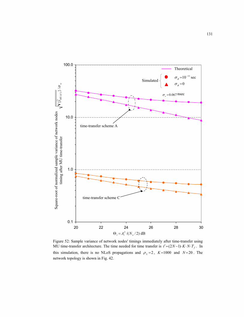
131
0.1
1.0
10.0
100.0
20 22 24 26 28 30
Figure 52: Sample variance of network nodes' timings immediately after time-transfer using MU time-transfer architecture. The time needed for time transfer is fTNKNt ⋅⋅⋅−=′ )12( . In this simulation, there is no NLoS propagations and 2=Lρ , 1000=K and 20=N . The network topology is shown in Fig. 42.
)2//(2ott NA=Θ dB
time-transfer scheme A
time-transfer scheme C
Squa
re-r
oot o
f nor
mal
ized
sam
ple
varia
nce
of n
etw
ork
node
s tim
ing
afte
r MU
tim
e-tra
nsfe
r
wk
MU
tσ/
~ )'
(V
Theoretical
Simulated 1110 −=φσ sec
0=φσ
067.0=wσ nsec
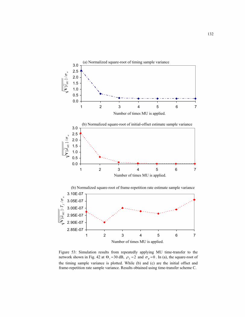
132
Figure 53: Simulation results from repeatedly applying MU time-transfer to the network shown in Fig. 42 at 30=Θ t dB, 2=Lρ and 0=φσ . In (a), the square-root of the timing sample variance is plotted. While (b) and (c) are the initial offset and frame-repetition rate sample variance. Results obtained using time-transfer scheme C.
0.00.51.01.52.02.53.0
1 2 3 4 5 6 7
Number of times MU is applied.
w
MU
tσ/
~ V
(a) Normalized square-root of timing sample variance
0.00.51.01.52.02.53.0
1 2 3 4 5 6 7Number of times MU is applied.
wM
Ud
σ/~
V
(b) Normalized square-root of initial-offset estimate sample variance
2.85E-07
2.90E-07
2.95E-07
3.00E-07
3.05E-07
3.10E-07
1 2 3 4 5 6 7Number of times MU is applied.
(b) Normalized square-root of frame-repetition rate estimate sample variance
w
fM
UT
aσ/
~
⋅V
133
6.1.2 Simulations with Random Network Topology
It is of interest to examine the ensemble average performances of the various time-transfer
architectures when the network nodes are randomly distributed in a given area.
We let the x and y co-ordinates of the network nodes to be uniformly distributed between 0
to 20 meters while fixing the lead master node at location (0, 20), i.e., the lead master node is at the
upper left-hand-corner of Fig. 42. At each Monte Carlo's step, the network nodes occupied new
locations within a square of 20x20 meters and take on new values of initial offset and frame repetition
rate. In these simulations, no receiver error is assumed, i.e., 0~, =smρ .
The simulation results are plotted in Figs. 54 to 56. The initial offset and η are uniformly
distributed within ±0.5x10⁻⁹ and between 1x10⁻⁶ to 10x10-6 respectively except the lead master node
which has η=0. No NLoS propagation is introduced into the simulation and when HM is employed,
the number of roving masters is N-1. The timing error and timing variances are computed using the
analytical equations presented in Chapter 5.
Note that when oscillator phase noise is negligible, i.e., 0=φσ , the sample variance of the
timings of all nodes in the network after MU time-transfer is close to the maximum timing error
variance obtained via HM time-transfer with 1−N roving masters (including the lead master node).
The maximum timing error variance for a network of N nodes after HM time-transfer is defined as
Ns
skHMk tt 2
)()'(
)1()'( ~max =−V . Similarly the minimum timing error variance is defined as
Ns
skHMk tt 2
)()'(
)1()'( ~min =−V .
If 1110 −=φσ sec, 067.0=wσ nanosecond and at sufficient SNR so that measured ToAs are
not overwhelmed by noise, the sample variance after MU time-transfer is close to the minimum
timing error variance obtained via HM time-transfer.

134
The better performance of MU compared to HM when oscillator phase noise is significant
can be explained by the fact that timing error variances are accumulated from one roving master to
another in the HM time-transfer architecture. The non-zero oscillator's timing jitter is propagated
through the network leading to higher timing error variances in individual nodes in the HM time-
transfer architecture.
1
10
100
1000
20 22 24 26 28 30
1
10
100
1000
20 22 24 26 28 30
1
10
100
1000
20 22 24 26 28 301
10
100
1000
20 22 24 26 28 30
Figure 54: Normalized timing/timing error standard deviation when co-ordinates of the network nodes are uniformly distributed and utilizing time-transfer scheme A for transmitted SNR from 20 dB to 30 dB. In (a) and (b), σφ=0 while in (c) and (d), σφ=10-11 sec. Here =wσ 0.067 nsec.
)2//(2ott NA=Θ dB )2//(2
ott NA=Θ dB w
sk
HM
kt
tσ/
)~
(2
)(
)'(
)1()'
(−
Ε fo
r HM
, w
kM
Ut
σ/~
)'(
V fo
r MU
w
sk
HM
kt
tσ/
)~
(2
)(
)'(
)1()'
(−
Ε fo
r HM
, w
kM
Ut
σ/~
)'(
V fo
r MU
(a) (c)
)2//(2ott NA=Θ dB )2//(2
ott NA=Θ dB w
sk
HM
kt
tσ/
)~
(2
)(
)'(
)1()'
(−
Ε fo
r HM
, w
kM
Ut
σ/~
)'(
V fo
r MU
w
sk
HM
kt
tσ/
)~
(2
)(
)'(
)1()'
(−
Ε fo
r HM
, w
kM
Ut
σ/~
)'(
V fo
r MU
(b) (d)
HM, N=40
max mean min
HM, N=20
max mean min
MU, N=40 MU, N=20
HM, N=40
max mean min
HM, N=20
max mean min
MU, N=40 MU, N=20
HM, N=50
max mean min
HM, N=30
max mean min
MU, N=50 MU, N=30
HM, N=50
max mean min
HM, N=30
max mean min
MU, N=50 MU, N=30
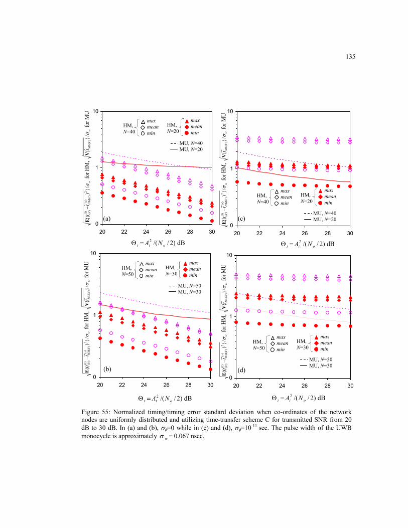
135
Figure 55: Normalized timing/timing error standard deviation when co-ordinates of the network nodes are uniformly distributed and utilizing time-transfer scheme C for transmitted SNR from 20 dB to 30 dB. In (a) and (b), σφ=0 while in (c) and (d), σφ=10-11 sec. The pulse width of the UWB monocycle is approximately =wσ 0.067 nsec.
0
1
10
20 22 24 26 28 30
)2//(2ott NA=Θ dB
w
sk
HM
kt
tσ/
)~
(2
)(
)'(
)1()'
(−
Ε fo
r HM
, w
kM
Ut
σ/~
)'(
V fo
r MU
(a)
0
1
10
20 22 24 26 28 30
)2//(2ott NA=Θ dB
w
sk
HM
kt
tσ/
)~
(2
)(
)'(
)1()'
(−
Ε fo
r HM
, w
kM
Ut
σ/~
)'(
V fo
r MU
(d) 0
1
10
20 22 24 26 28 30
)2//(2ott NA=Θ dB
w
sk
HM
kt
tσ/
)~
(2
)(
)'(
)1()'
(−
Ε fo
r HM
, w
kM
Ut
σ/~
)'(
V fo
r MU
(b)
0
1
10
20 22 24 26 28 30
)2//(2ott NA=Θ dB
w
sk
HM
kt
tσ/
)~
(2
)(
)'(
)1()'
(−
Ε fo
r HM
, w
kM
Ut
σ/~
)'(
V fo
r MU
(c)
HM, N=40
max mean min
HM, N=20
max mean min
MU, N=40 MU, N=20
HM, N=40
max mean min
HM, N=20
max mean min
MU, N=40 MU, N=20
HM, N=50
max mean min
HM, N=30
max mean min
MU, N=50 MU, N=30
HM, N=50
max mean min
HM, N=30
max mean min
MU, N=50 MU, N=30

136
Figure 56: Normalized timing/timing error standard deviation when co-ordinates of the network nodes are uniformly distributed and utilizing time-transfer scheme C for transmitted SNR from 40 dB to 50 dB. In (a) and (b), σφ=0 while in (c) and (d), σφ=10-11 sec. The pulse width of the UWB monocycle is approximately =wσ 0.067 nsec.
0.01
0.10
1.00
10.00
40 42 44 46 48 50
)2//(2ott NA=Θ dB
w
sk
HM
kt
tσ/
)~
(2
)(
)'(
)1()'
(−
Ε fo
r HM
, w
kM
Ut
σ/~
)'(
V fo
r MU
(a)
0.1
1.0
10.0
40 42 44 46 48 50
)2//(2ott NA=Θ dB
w
sk
HM
kt
tσ/
)~
(2
)(
)'(
)1()'
(−
Ε fo
r HM
, w
kM
Ut
σ/~
)'(
V fo
r MU
(d) 0.01
0.10
1.00
10.00
40 42 44 46 48 50
)2//(2ott NA=Θ dB
w
sk
HM
kt
tσ/
)~
(2
)(
)'(
)1()'
(−
Ε fo
r HM
, w
kM
Ut
σ/~
)'(
V fo
r MU
(b)
0.1
1.0
10.0
40 42 44 46 48 50
)2//(2ott NA=Θ dB
w
sk
HM
kt
tσ/
)~
(2
)(
)'(
)1()'
(−
Ε fo
r HM
, w
kM
Ut
σ/~
)'(
V fo
r MU
(c)
HM, N=40
max mean min
HM, N=20
max mean min
MU, N=40 MU, N=20
HM, N=40
max mean min
HM, N=20
max mean min
MU, N=40 MU, N=20
HM, N=50
max mean min
HM, N=30
max mean min
MU, N=50 MU, N=30
HM, N=50
max mean min
HM, N=30
max mean min
MU, N=50 MU, N=30
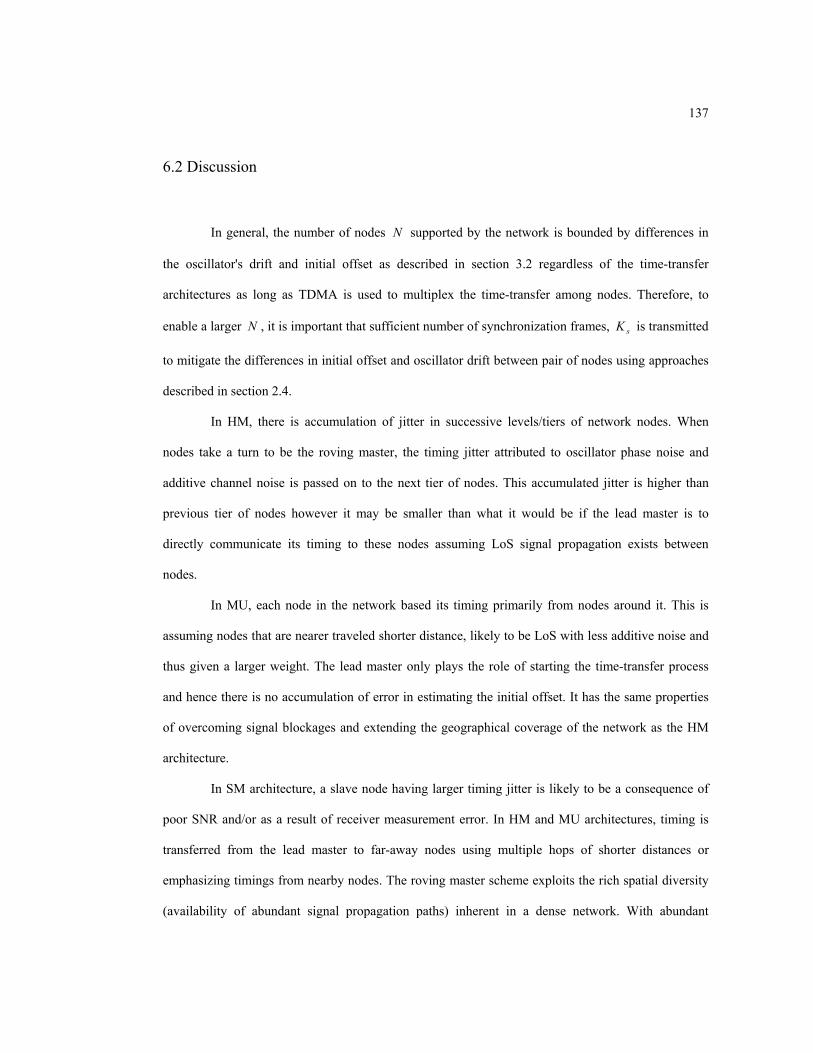
137
6.2 Discussion
In general, the number of nodes N supported by the network is bounded by differences in
the oscillator's drift and initial offset as described in section 3.2 regardless of the time-transfer
architectures as long as TDMA is used to multiplex the time-transfer among nodes. Therefore, to
enable a larger N , it is important that sufficient number of synchronization frames, sK is transmitted
to mitigate the differences in initial offset and oscillator drift between pair of nodes using approaches
described in section 2.4.
In HM, there is accumulation of jitter in successive levels/tiers of network nodes. When
nodes take a turn to be the roving master, the timing jitter attributed to oscillator phase noise and
additive channel noise is passed on to the next tier of nodes. This accumulated jitter is higher than
previous tier of nodes however it may be smaller than what it would be if the lead master is to
directly communicate its timing to these nodes assuming LoS signal propagation exists between
nodes.
In MU, each node in the network based its timing primarily from nodes around it. This is
assuming nodes that are nearer traveled shorter distance, likely to be LoS with less additive noise and
thus given a larger weight. The lead master only plays the role of starting the time-transfer process
and hence there is no accumulation of error in estimating the initial offset. It has the same properties
of overcoming signal blockages and extending the geographical coverage of the network as the HM
architecture.
In SM architecture, a slave node having larger timing jitter is likely to be a consequence of
poor SNR and/or as a result of receiver measurement error. In HM and MU architectures, timing is
transferred from the lead master to far-away nodes using multiple hops of shorter distances or
emphasizing timings from nearby nodes. The roving master scheme exploits the rich spatial diversity
(availability of abundant signal propagation paths) inherent in a dense network. With abundant

138
alternative network signal propagation paths to propagate timing from one node to another, time
transfer can be performed via multiple intermediate nodes for which it is with high probabilities the
links between nodes are LoS signal propagation paths. Therefore the SIN with roving masters does
not present new algorithms to mitigate timing error arising from NLoS signals between pair of nodes
per se. Its intention is to select the propagation path with the smallest measured timing jitter and
possibly complement the many works already available in the literature such as [3], [64], [67] and
[71] that described how to discern and handle the presence of NLoS signals in a multipath
environment.
In [67], where multiple receivers are used to locate the position of a radio frequency source,
the fact that the difference between NLoS and LoS propagations are always positive is used to
constraint the domain over which mathematical programming is used to find the ML estimate of the
source position. A similar technique is used in [64], which estimates are based on a constrained
nonlinear optimization problem derived from the topology of the system. A more heuristic approach is
used in [71] that discriminates between LoS versus NLoS measurements using the time history of the
range measurements and corrects the NLoS ranging error by exploiting apriori knowledge of the
statistical characteristics of the system's standard measurement noise. The approach adopted in [3] is
to apply the maximum likelihood expectation-maximization and Bayesian estimators to estimate the
LoS distance between transmitter and receiver, given the probability density function of the ToA
which is derived from a multipath scattering model.
On first inspection, the results presented in Figs. 43 to 51 seem to indicate that SM has the
lowest timing jitter among the three different time-transfer architectures for all nodes in the network.
The simulations and theoretical analysis are based on the assumption that the measurement system, in
particular, the AGC and the timing detector operate at received SNR above 15 dB. However, the
transmitted SNR (defined as )2//(2ott NA=Θ ) is related to the received SNR by
)(log10 ,10, smLtsm D⋅⋅−Θ=Θ ρ . If 2=Lρ and 30=Θ t dB, a node 10 meters away from the lead
139
master node would have a received SNR of 10, =Θ sm dB. This violates the earlier assumption that the
measurement system operates at 15, ≥Θ sm dB. As illustrated in Chapter 2, when 15, <Θ sm dB, the
AGC may not be able to regulate the amplitude of the received UWB monocycle and as a result the
timing detector may not be operating at the tracking mode (linear portion of its characteristic
function). The assumption that 15, ≥Θ sm dB is easily met for HM and MU since each roving master
will be transmitting at tΘ . Hence, when there is a constraint to the maximum power that the master
node can transmit, HM is a better choice than SM. In Fig. 57, the receiver SNR at node s relative to
the transmitted SNR of the lead master node is illustrated.
The simulation results on random network demonstrated the characteristic of the MU time-
transfer architecture. When 0=φσ or is negligible (when a highly stable oscillators are utilized), the
HM outperforms the MU. For the range of SNR simulated, the sample timing variance of MU is not
better than the node in the HM architecture that has the poorest timing jitter. However, when φσ is
0
5
1 0
1 5
2 0
0 5 1 0 1 5 2 0
1
2
3
4
5
6
7
8
9
1011
12
13
14 15
16
17
1819
20
30=Θ t dB
10, =Θ sm dB
98.3, =Θ sm dB
46.1, =Θ sm dB
(meters)
(meters)
Figure 57: Illustration of the relationship between transmitter and receiver SNR. In order for node 9 to have received SNR of 15, =Θ sm dB, node 1 needs to transmit at
5.43=Θ t dB.

140
significant, the sample timing variance of MU is close to the timing jitter of the node in the HM with
the smallest timing jitter. This is because when φσ is significant relative to additive channel noise,
nodes in HM are not able to select roving master nodes based on links that have the smallest ToA
variances. Further more, the oscillator phase noise propagates and accumulates through the network.
The inability to select roving master node based on link quality and accumulation of oscillator phase
noise degrades the performance of HM time-transfer architecture significantly especially for nodes
that only acquired their timings after multiple roving master sessions.
If only ),()(
smvSYΩ and ),(
)(ms
uUPΩ are measured at s and m respectively, time-transfer can still be
performed via two-way time-transfer [58], noting that ),()(
smzSYΩ and ),(
)(ms
uUPΩ have smaller measurement
noise than ),()(
smzDNΩ . However, to complete the time-transfer, measurements obtained at s and m have
to be encoded into information bits and exchanged using additional wireless resources. When
extended to network synchronization, it is likely that the pair-wise two-way time-transfer involves
more resources from higher layers (above the physical layer) with timing latency that is harder to
predict than the proposed scheme.
The proposed synchronization scheme is similar to the RTS [33] [34] because both use a
forward path and two return paths for propagation delay mitigation. However, RTS requires N2
phase detectors per node, which may not be practical for UWB signals.
It should also be noted that [39] has used linear regression (LS) to estimate the frame
frequency differences and it is also mentioned in [15] as a possible way to correct the frame frequency
differences.
Using [34] as a checklist, the proposed SIN exhibits most of the said advantages such as
"decentralized timing control" and "each network node has equivalent influence" for MU and "stable"
for HM. It should be noted that the objective of HM is different from MU. In HM, it is desired to have
the timing of all nodes in the network to follow as closely as possible to the timing of a designated
141
master node. For MU, one of its objectives is to prevent the failure of network node/s from affecting
the performance of the synchronous network severely.
In a SM network, the time needed for synchronization is fKTN )1(2 − seconds. The HM with
mQ roving master (including lead master) needs mf QKTN ⋅− )1(2 seconds while MU needs
NKTN f)1(2 − seconds to synchronize all nodes in the network. Among the three time-transfer
architectures, the HM involves more computation and concerted effort is needed to select, assign and
let the other nodes know which node is the next roving master. This involves higher layer network
protocol and is not the subject of investigation in this work.
142
CHAPTER VII
CONCLUSIONS
7.1 Conclusions
In this section, the works accomplished and the performance of SIN and its practical
applications are summarized.
(a) Works Accomplished
A synchronous impulse network (SIN) realized with the proposed time-division-multiplex
synchronizing scheme and its variations are the subject of this research. The nodes in the network are
time synchronized using the master-slaves (SM), hierarchical master-slaves (HM) or mutually
synchronous (MU) time-transfer architectures.
In Chapter 2, we have comprehensively analyzed the correlative timing detector that is used
to measure the ToA of UWB monocycles at the receiver in the presence of additive channel noise,
oscillator phase noise, multipath self-interference and NLoS propagations. Chapter 3 presented
(i) the proposed time-transfer schemes (time-transfer schemes A, B and C),
(ii) the LS estimator to estimate the frame frequency differences followed by
(iii) two-way ranging to estimate the differences in initial offset among network nodes, and
(iv) evaluated the number of nodes supported in the network.
Chapter 4 introduces the roving master concept for time-transfer and evaluated the performances of
the SM, HM and MU time-transfer architectures in implementing the SIN. The variances of the timing
errors are presented in Chapter 5 and Chapter 6 reported the simulation results.
A summary of works accomplished in this research is shown in Fig. 58.
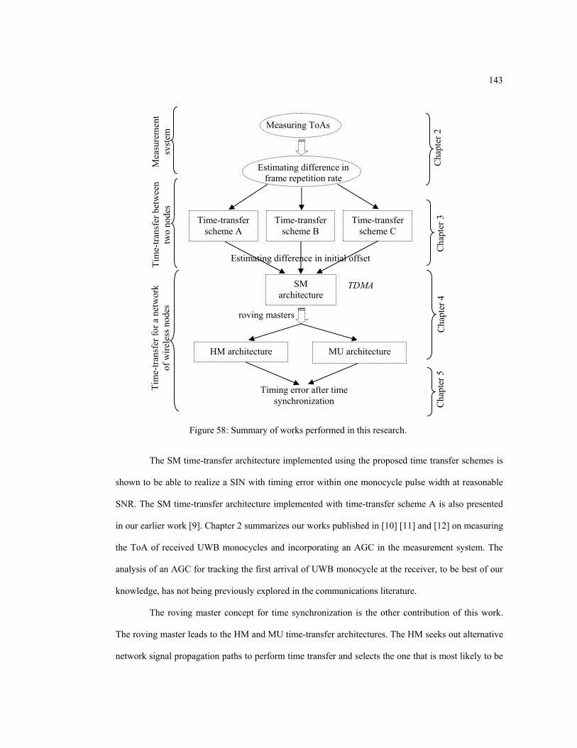
143
The SM time-transfer architecture implemented using the proposed time transfer schemes is
shown to be able to realize a SIN with timing error within one monocycle pulse width at reasonable
SNR. The SM time-transfer architecture implemented with time-transfer scheme A is also presented
in our earlier work [9]. Chapter 2 summarizes our works published in [10] [11] and [12] on measuring
the ToA of received UWB monocycles and incorporating an AGC in the measurement system. The
analysis of an AGC for tracking the first arrival of UWB monocycle at the receiver, to be best of our
knowledge, has not being previously explored in the communications literature.
The roving master concept for time synchronization is the other contribution of this work.
The roving master leads to the HM and MU time-transfer architectures. The HM seeks out alternative
network signal propagation paths to perform time transfer and selects the one that is most likely to be
Time-transfer scheme A
Time-transfer scheme B
Time-transfer scheme C
SM architecture
HM architecture MU architecture
Measuring ToAs
Estimating difference in frame repetition rate
Estimating difference in initial offset
roving masters
Timing error after time synchronization
Cha
pter
2
Cha
pter
3
Cha
pter
4
Cha
pter
5
Tim
e-tra
nsfe
r bet
wee
n tw
o no
des
Mea
sure
men
t s y
stem
Ti
me-
trans
fer f
or a
net
wor
k of
wire
less
nod
es
Figure 58: Summary of works performed in this research.
TDMA
144
a LoS path. The main objective is to avoid time transfer via NLoS signal propagation paths. A signal
received via a NLoS propagation path has lower SNR due to the longer propagation distance
compared to a LoS signal. The MU averages the timings of nodes in the network.
(b) SIN Performance
For a given path-loss exponent and time-transfer architecture, time-transfer scheme C
achieves the lowest timing error variances while time-transfer scheme A has the highest timing error
variance. (Fig. 22)
Assuming the received SNR is above 15 dB and employing a specific time-transfer scheme
(A, B or C), the relative performance between SM, HM and MU time-transfer architectures depends
on the path-loss exponent and the network topology. In general, the timing jitter in HM will be close
to that achieves by SM for a channel with larger path-loss exponent or a network covering a larger
area with few roving mater nodes. (Figs. 38 and 39)
Assuming a path-loss exponent of 2=Lρ , it is observed that if time-transfer is via LoS
propagation and oscillator phase noise is negligible compared to timing jitter introduced by additive
channel noise, the SM architecture achieves the lowest timing error variance at a given SNR. The HM
architecture has the second lowest timing error variance while the MU has the highest timing sample
variance. (Figs. 50 and 51)
The other objective of extending the geographical coverage of the synchronous network
using roving masters is hindered by the need to have a TDMA scheme to multiplex time transfer
among nodes. The proposed roving master concept requires nodes to take a turn as the master node.
This extends the time horizon needed to perform time transfer/synchronization. In the presence of
residual error in frame frequency (drift fT× ) difference estimation, a longer synchronization time
multiplied with the frame frequency estimation error leads to larger timing errors and jitter.
145
This work has demonstrated that, ignoring φσ , it is possible to achieve a synchronous
impulse network with timing jitter in the order of the pulse width of a UWB monocycle, for example,
node 8 in Figs. 50 and 51, and the results shown in Fig. 41.
(c) Applications
From section 6.2, we observed that if the objective of time synchronization is to ensure
minimum timing jitter, then taking into consideration the fact that the measurement system (consisting
of AGC and correlative timing detector) is to operate at received SNR above 15 dB, the SM time-
transfer architecture should be the appropriate option when there are many nodes in the network
occupying a small area (e.g. 10x10 meters and smaller). Possible applications include array-beam
forming and reach-back communications if these nodes are deployed in a small localized area.
For a network covering a wider area, HM time-transfer architecture should be utilized. The
HM architecture is well-suited for application like geo-locationing. In this application, multiple
receivers (nodes that perform the task of locating the emitter/s) are usually placed in fixed known
locations. Then a HM roving master scheme can be devised easily to ensure small timing jitter. For
example, if the distances between nodes are known a priori, it is possible to pre-determine the order of
the roving master node. This minimizes un-certainties in assigning roving master nodes and generally
produces lower timing jitter.
If the network nodes need to be in-expensive and are implemented with oscillators that have
high phase noise, the MU is a better choice than HM. The MU fits well in application such as sensor
networks when the nodes are expected to be cheap, and the nodes formed an ad hoc network with no
preferred nodes. Moreover, in most practical situations, the physical phenomenon to be sensed does
not require network nodes to have very fine timing resolutions. The need of timing precision in the
order of nanoseconds offered by SM and HM architectures described in this work usually does not
arise.

146
If many nodes are deployed in a large geographical area, to avoid the long synchronization
time of the roving masters approach, dividing the network into smaller area and employing a mixture
of SM, HM and MU time-transfer architectures should be a better engineering solution than trying to
deploy a SIN with only one type of time-transfer architecture.
(d) Research Contributions
This research has proposed a time-transfer scheme (and its variations) to establish a
synchronous impulse network utilizing UWB impulse radio. The ultra-wide bandwidth of UWB
signals is exploited to enable a synchronous impulse network achieving timing precision, i.e. timing
differences among network nodes, in the order of nanoseconds. This compared favorably with timing
precision reported in the review paper [56], which reported various timing synchronization schemes
archiving precision in the order of microseconds.
The proposed roving master concept for time-transfer exploited the "richness" (availability)
of alternate network signal propagation paths in the HM architecture to avoid time-transfer via NLoS
paths, and enable a MU architecture that attempts to average out the effect of NLoS propagation error.
We have derived analytical results for multi-hops time synchronization taking into
consideration the effect of frame-repetition rate differences between network nodes. Thus filling the
gap mentioned in [56] that there is a 'lack of analytical models for multi-hop synchronization'.
However, we should note that [34] has formulated analytically a HM time-transfer architecture for a
FDMA scheme that utilizes a closed-loop phase detector for time synchronization. The effect of
frame-repetition rate differences is not considered in [34].
The proposed synchronization scheme can be modified to suit some narrowband
communication systems. Note that mulitpath self-interference may then have to be taken into account
when evaluating the performance of the synchronous system.

147
7.2 Future Research
This work has not, in its humble length of approximately 100 pages, been able to
exhaustively analyze and address all issues involved in establishing a SIN. The following is a list of
possible issues that we feel will enhance the usefulness of this work. This list of possible future
research topics is broadly grouped into separate headlines, namely: estimation techniques, effect of
network topology, ranging, and a summary of restrictive assumptions that are made in this work.
7.2.1 Estimation Techniques
The techniques used to estimate the initial offset and frame repetition rate differences are
under the realm of "classical" techniques. The Least Squares estimator used to estimate the
differences in frame repetition rate between a pair of nodes can be shown to approach the Cramer Rao
lower bound for a stationary AWGN channel [13]. The ToAs are measured at the output of the open
loop timing detector, and there is no tracking of timing jitter.
Incorporating a tracking loop will help to deal with variations in the wireless channels and
possibly improve the performance of the time-transfer. If the oscillator phase jitter is to be modeled as
a Gauss-Markov process, iterative techniques such as those mentioned in [61] to track the phase jitter,
are likely to improve the performance of the time-transfer.
Other estimation techniques such as Kalman filtering, expectation-maximization are not
investigated in this work.
When the received SNR is below 15 dB, it is shown in Chapter 2 that the AGC may not be
able to regulate the amplitude of the received UWB monocycle effectively. As a result, the timing
detector may not be operating in the linear portion of its characteristic function. This will degrade the
performance of the time-transfer schemes. A more comprehensive analysis of the working of the
AGC at lower SNR is left to future work.

148
There possibly exist other approaches to utilizing the ToA measurements to estimate the
differences in initial offset and drift. There are also possible ways to enhance the performance of the
proposed time-transfer scheme. For example, at the end of each roving-master session, the slave node
can utilize the measured ToAs of the frame-synchronizing pulses, ),()(
smvSYΩ and downlink ranging
pulses, ),()(
smzDNΩ to re-estimate the difference in frame repetition rate between itself and the master
node. To avoid exhaustively analyzing all possible alternative approaches, a more efficient analytical
technique, such as graph theory, is needed.
7.2.2 Effect of Network Topology
(a) Graph Theory and Network Topology
The performances of the various time-transfer architectures depend on the network topology.
To aid in choosing the "optimal" time-transfer architecture for a specific application, a statistical
description of the performances of the various time-transfer architectures for an arbitrary network
topology will be useful. The modeling of an arbitrary network topology with nodes randomly
distributed in a given area with links that may or may not be LoS has not been addressed in this work.
A recent work [26], which modeled sm,ρ and ms,ρ as random variables with exponential
distribution of mean ρ , has derived an unbiased ML estimator for )()(),( smsm ddd −=δ . Assuming
)()( sm aa = , and ignoring additive channel noise and oscillator phase noise, the ML unbiased estimator
for ),( smdδ is ( ) 2/)(min)(minˆ 10
),()(
10
),()(
),( −=
−= Ω−Ω= K
ksmuUP
Kk
smvSY
sm kkdδ with variance 22/ Kρ . This result
may help in devising addition signal processing techniques to further mitigating the bias introduced
by NLoS propagation.

149
To investigate the performance of a network of randomly distributed nodes, graph theory
maybe a useful tool. From [30], a simple graph is defined as,
"a triple ),,( IEVG= where V and E are disjoint finite sets and I is an incidence
relation such that every element of E is incident with exactly two distinct elements of
V and no two elements of E are incident to the same pair of elements of V . "
Sets V and E are known as the vertex and edge sets of G respectively. Then it is possible to
represent nodes in the network as elements of the vertex set, and two nodes are joined by an edge E∈
if it is possible for one to communicate with the other.
(b) Minimum Energy Network
In [29] and [52], graph theory is used to devise network protocols to establish a 'minimum
energy network' for wireless communications. The proposed network protocol finds the minimum-
energy path between m and s , assuming a communication link between m and s is feasible. In this
context, the minimum energy path is defined as one that allows messages to be transmitted with a
minimum use of energy. The protocol is devised making use of the fact that power required to
transmit from m to s is governed by the path-loss exponent 2≥Lρ in ( ) LsmD ρ
, where smD , is the
distance traveled by the signal propagating from m to s in meters. Therefore it is possible to relay
information from m to s via intermediate node/s with less power than to transmit directly from m to
s . For the protocol to establish a minimum energy network, both [29] and [52] require each node to
know its location. This is made possible by assuming that nodes in the network are each equipped
with a GPS receiver.
If we view the shortest propagation path as being equivalent to the minimum energy path for
communications [29] [52], there seems to be close resemblance between constructing a minimum
energy network and establishing a synchronous impulse network with minimum timing error. In fact,

150
exploiting the properties of the path loss exponent is a feature of the proposed roving-master time-
transfer concept. The possibilities of drawing on results reported in [29] [52] to analyze the proposed
synchronous impulse network are left to future research. There may be other works in
computer/information and networking technologies, such as network scheduling that may be utilized
to improve or analyze the performance of the proposed time synchronization schemes.
(c) Multiple Roving Masters per Time-transfer Session
This work analyzed the case whereby each node takes a turn as the roving master, i.e., only
one node is being assigned as the 'master' while other nodes are slaves at any point in time. It is
possible that the current master node estimates the variances of the measured ToA of impulses from
other nodes in the network and appoints multiple nodes to be the next tier of roving masters by
grouping nodes with similar measured ToA variances. This "tree-like" HM time transfer architecture
is illustrated in Figs. 59 and 60. Obviously more could be accomplished with more resources
expended at each node to co-ordinate this 'tree-like' architecture instead of the "thread-like"
hierarchical master-slave time-transfer architecture investigated in this work.
If the topology of the network is known, the performance of the network depicted in Fig. 59
can be predicted using analytical expressions presented in Chapters 4 and 5.
(d) Optimality of Time-Transfer Scheme
The optimality of the proposed time-transfer scheme has not been fully addressed in this
work. The design of the proposed time-transfer scheme is guided by implementation considerations,
for example, TDMA is the natural choice instead of FDMA because UWB signals occupied very large
bandwidth.
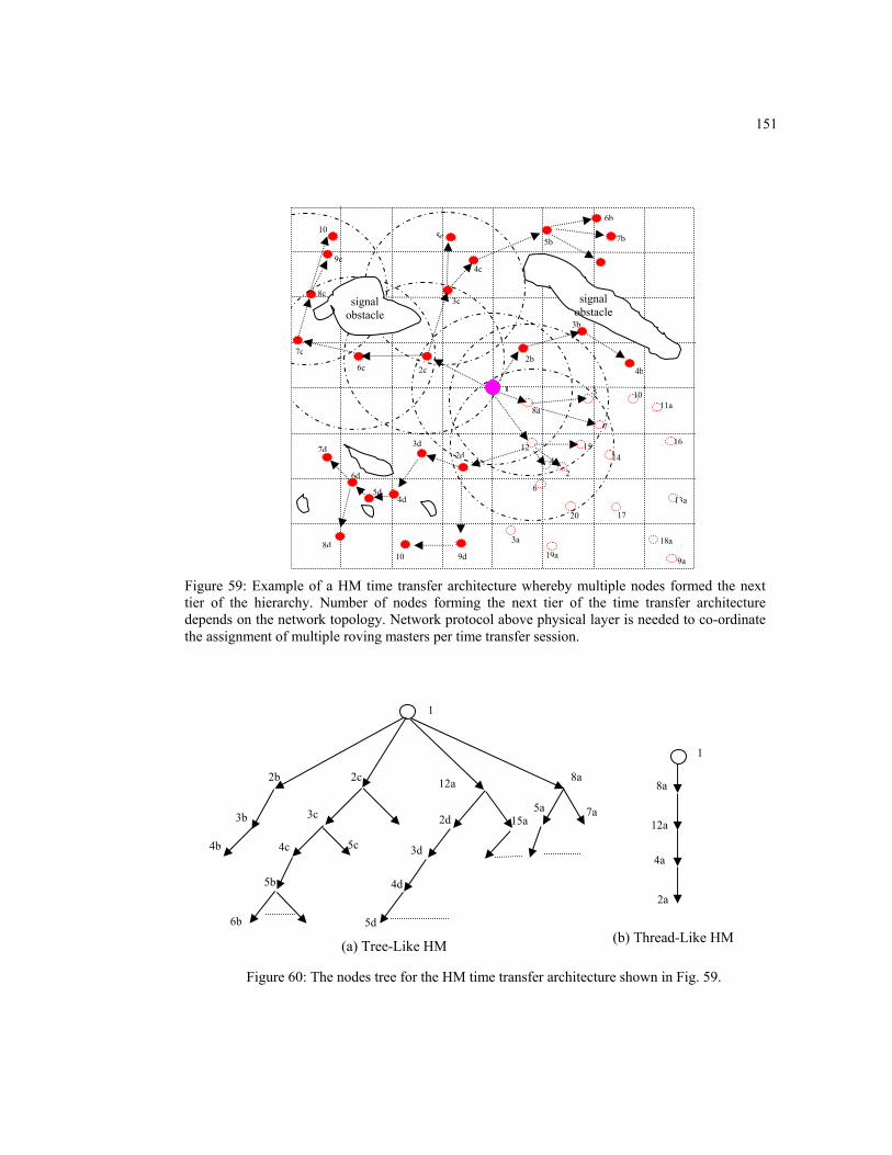
151
Figure 59: Example of a HM time transfer architecture whereby multiple nodes formed the next tier of the hierarchy. Number of nodes forming the next tier of the time transfer architecture depends on the network topology. Network protocol above physical layer is needed to co-ordinate the assignment of multiple roving masters per time transfer session.
1
2
3a
4
5
6
7
8a
9a
1011a
12
13a
1415 16
17
18a 19a
20
108d
4d
9d
2d3d
5d
6d
7d
2c
3c
4c
5c
6c
7c
8c
9c
10
2b
3b
4b
5b
6b
7b
signal obstacle
signal obstacle
1
2b
3b
4b
2c
3c
4c 5c
5b
6b
12a 8a
2d
3d
4d
5d
15a 5a 7a
(a) Tree-Like HM
1
8a
12a
4a
2a
(b) Thread-Like HM
Figure 60: The nodes tree for the HM time transfer architecture shown in Fig. 59.

152
It is assumed that the first arrival is most probably a LoS path and possibly offers the best
signal for measuring the ToA. In practice, the first discernible signal at the receiver may be a signal
that arrives via a NLoS propagation path.
In HM time-transfer architecture, the order of time-transfer is dictated by the shortest signal
propagation path. The shortest signal propagation path is assumed to correspond to the signal
propagation path with measured ToAs that has the smallest variance.
In MU time-transfer architecture, timing information obtained from the shortest path is
emphasized (given larger weight). Moreover, it is assumed that nodes take turns being the roving
master in the natural order if nodes are labeled as 1,2,3,… . It is likely that for a given network
topology, there may exist a preferred way to order the nodes when utilizing MU time-transfer
architecture to achieve minimum timing error variance. The optimal order has not being investigated
in this work.
Choosing the shortest network signal propagation paths or emphasizing timings associated
with these paths has not being proven to bring about a globally optimal system with the smallest
timing error for all nodes in the network. Intuitively, choosing the link with the shortest propagation
delay for time transfer will likely lead to smaller timing error.
7.2.3 Restrictive Assumptions
In this work, nodes are assumed stationary which considerably simplifies estimating the
difference in frame repetition rate between nodes. In a practical application, such as operating on a
mobile platform, there is a need to consider the effect of compression and expansion of UWB signals.
After introducing the synchronization scheme, the derivations that followed assume the
indices of the uplink i and downlink j time slots is such that ji= for every node in the network.
This introduces "regularity" in the network and simplifies the analysis. The regularity refers to the fact
that the characteristic function of the time-transfer scheme )(kθ in (3.12) will then only be a function

153
of N and K for all nodes in the network. A larger ji− will increase the error in estimating the
difference in initial offset for the pair of nodes with uplink index i and downlink index j . The
existence of an optimal way of assigning the time slots index i and j that will reduce the timing
error in the network is not addressed here.
The number of synchronization frames is assumed to be equal to the number of ranging
frames. Allocating different numbers of frames for frame repetition rate synchronization and ranging
estimation may lead to a more power efficient time-transfer scheme. This is because error variance for
frame repetition rate estimation decreases asymptotically in the order of 3K while initial offset
estimation variances decreases only in the order of K .
The path-loss exponent is assumed to be 2 in our performance analysis. A higher path-loss
exponent may make HM performs better than the SM time-transfer architecture. In Chapter 5, Figs.
37 to 39, an analysis using a "straight" line topology, i.e., nodes in the network are arranged in a
straight line, shows that indeed a higher path-loss exponent will bring the timing error variance of HM
closer to that of SM.
In the MU time-transfer architecture simulations, the weight sm,α is constructed via the
function ∑≠=
ΩΩ=N
smm
smzDN
smzDNsm
',1'
),'()(
),()(, /1/1 VVα . It is not known whether other weight
functions, for example, ∑≠=
Ω−Ω−=N
smm
smzDN
smzDNsm
',1'
),'()(
),()(, )exp()exp( VVα , or employing higher
order polynomial, would yield a lower timing jitter. In Chapter 5, Fig. 40, the timing variances using 3
different weight functions are evaluated analytically for the network topology shown in Fig. 42. For
this example, no significant differences in timing variances using the 3 weight functions defined in
Fig. 40 is observed.
Last but not least, no stability analysis is performed in this work. Here, "stability" means
timing error does not increase without bound after application of time transfer. Although HM is likely
to be stable, as timing information is passed from the lead master to other nodes in the network in one

154
direction with no feedback. The stability of MU is of concern if it is to be applied repeatedly since
timing information is transferred back and forth through the network.
To expand the number of nodes that can be supported by the proposed synchronization
scheme, each network of N nodes can be described as a single "cell" and a higher layer network
protocol may be used to connect cells together to form an extended network.
An obvious disadvantage of the proposed synchronization scheme is that transceivers in the
network are assigned specific time slot, thus it is difficult to dynamically add or remove transceivers
from the network. To mitigate this shortcoming, protocols above physical layer may be needed.
7.2.4 Ranging and Geo-locationing
This work is about synchronizing the timing of network nodes. A by-product of the proposed
time synchronization scheme is range information between pair of nodes. The range information
between pair of nodes can be derived/estimated from the ToA of the downlink ranging pulses. From
(3.21),
mssmmssmsm
zDN ,,,,),(
)( ρρττ +++=ΩΕ ,
and
)()()( 2),()(
22),(),()(
smzDN
smsmzDN uz
LSεε γ ΕΕV +−⋅=Ω .
This can be expanded further to geo-locating of network nodes. It will be interesting to examine the
performance of ranging and the precision in estimating the co-ordinates of nodes achievable using the
proposed time synchronization scheme.
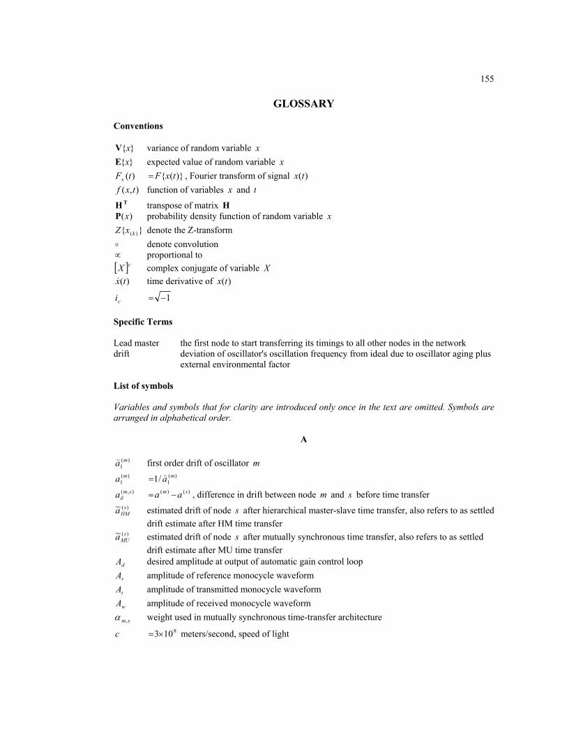
155
GLOSSARY
Conventions
xV variance of random variable x xΕ expected value of random variable x )(tFx )( txF= , Fourier transform of signal )(tx ),( txf function of variables x and t
TH transpose of matrix H )(xP probability density function of random variable x
)(kxZ denote the Z-transform o denote convolution ∝ proportional to [ ]cX complex conjugate of variable X
)(tx& time derivative of )(tx
ci 1−= Specific Terms Lead master the first node to start transferring its timings to all other nodes in the network drift deviation of oscillator's oscillation frequency from ideal due to oscillator aging plus
external environmental factor
List of symbols Variables and symbols that for clarity are introduced only once in the text are omitted. Symbols are arranged in alphabetical order.
A
)(1
ma( first order drift of oscillator m )(
1ma )(
1/1 ma(= ),( smaδ )()( sm aa −= , difference in drift between node m and s before time transfer
)(~ sHMa estimated drift of node s after hierarchical master-slave time transfer, also refers to as settled
drift estimate after HM time transfer )(~ s
MUa estimated drift of node s after mutually synchronous time transfer, also refers to as settled drift estimate after MU time transfer
dA desired amplitude at output of automatic gain control loop
rA amplitude of reference monocycle waveform
tA amplitude of transmitted monocycle waveform
wA amplitude of received monocycle waveform
sm,α weight used in mutually synchronous time-transfer architecture
c 8103×= meters/second, speed of light

156
D
)(md(
initial offset of oscillator m with respect to true time 0=t before time-transfer )(md )(
1)( / mm ad ((
= ),( smdδ )()( sm dd −= , difference in initial offset between node m and s before time transfer ),(ˆ smdδ estimate of difference in initial offset ),( smdδ between nodes m and s
)(sdδ weighted average initial offset differences evaluated at node s )(~ s
HMd estimated initial offset of node s after hierarchical master-slave time transfer, also refers to as settled initial offset estimate after HM time-transfer
)(~ sMUd estimated initial offset of node s after mutually synchronous time transfer, also refers to as
settled initial offset estimate after MU time-transfer )(kθ characteristic function of time-transfer scheme
kKN r −⋅−= 2/)1( , time-transfer scheme A kNN ⋅−−−= )12(2/)1( , time-transfer scheme B
kN ⋅−−= )12(2/1 , time-transfer scheme C
smD , distance traveled by signal transmitted from node m to receiver s measured in meters
)(1 ∆ϕD first structure function of the phase noise process of oscillator
E
)(m,saε random variable representing difference in drift between two oscillators m and s after time-
transfer )(m,s
dε random variable representing difference in initial offset between two oscillators m and s after time-transfer
)()(
m,skxε zero mean random error at output of open loop timing detector
),( smSYε zero mean random error due to additive channel noise and oscillator phase noise when
measuring )(),()( ksm
vSYΩ ),()(
msuUPε zero mean random error due to additive channel noise and oscillator phase noise when
measuring )(),()( kms
uUPΩ ),()(
smzDNε zero mean random error due to additive channel noise and oscillator phase noise when
measuring )(),()( ksm
zDNΩ ),( sm
ϑε zero mean random error of timing equation )(),( ksmϑ ),(
ˆsm
dε zero mean error associated with determining the estimate ),(ˆ smdδ of ),( smdδ by averaging
)(),( ksmϑ over k )(m,s
γLSε zero mean error associated with determining the least squares estimate ),(ˆ sm
LSγ of ),( smγ
η η+=1)(1
ma
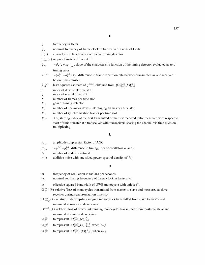
157
F
f frequency in Hertz
of nominal frequency of frame clock in transceiver in units of Hertz )(ςg characteristic function of correlative timing detector
)~(τMFg output of matched filter at τ~
TDg( 0
/)(=
=ς
ςς ddg , slope of the characteristic function of the timing detector evaluated at zero
timing error ),( smγ f
sm Taa ⋅−= )( )(1
)(1 , difference in frame repetition rate between transmitter m and receiver s
before time-transfer ),(ˆ sm
LSγ least squares estimate of ),( smγ obtained from 10
),()( )( −
=Ω Kk
smvSY k
i index of down-link time slot j index of up-link time slot K number of frames per time slot
DK gain of timing detector
rK number of up-link or down-link ranging frames per time slot
sK number of synchronization frames per time slot
STK 0≥ , starting index of the first transmitted or the first received pulse measured with respect to start of time-transfer at a transceiver with transceivers sharing the channel via time division multiplexing
L
SFΛ amplitude suppression factor of AGC
)(kµ )()( sk
mk φφ −= , difference in timing jitter of oscillators m and s
N number of nodes in network )(tn additive noise with one-sided power spectral density of oN
O
ω frequency of oscillation in radians per seconds oω nominal oscillating frequency of frame clock in transceiver 2ω effective squared bandwidth of UWB monocycle with unit sec-2.
)(),( ksmSYΩ relative ToA of monocycles transmitted from master to slave and measured at slave
receiver during synchronization time slot )(),(
)( kmsqUPΩ relative ToA of up-link ranging monocycles transmitted from slave to master and
measured at master node receiver )(),(
)( ksmzDNΩ relative ToA of down-link ranging monocycles transmitted from master to slave and
measured at slave node receiver ),( sm
SYΩ to represent 10
),()( )( −
=Ω Kk
smvSY k
),( msUPΩ to represent 1
0),()( )( −
=Ω Kk
msuUP k , when ji=
),( smDNΩ to represent 1
0),(
)( )( −=Ω K
ksm
zDN k , when ji=

158
p 22/1 wσ= , parameter of Gaussian derivative monocycle waveform
)()( tmϕ( random phase jitter of oscillator m )(
)(mkϕ( )()(
fm kTϕ(= , random phase jitter of oscillator m at fkTt=
)()( tmφ(
omm t ωϕϕ /))0()(( )()( ((
−= , in units of seconds )(
)(m
kφ(
omm
k ωϕϕ /)( )()0(
)()(
((−=
)()(
mkφ )(
1)(
)( / mmk a((φ=
P
)(tΦ total phase of oscillator in radians )( )(kςΨ auto-correlation function of UWB monocycle waveform evaluated at delay )(kς
Q number of hops from the lead master node to a particular roving master from which a slave node s acquires its timing
)(tr reference monocycle waveform generated at receiver
R
sm,ρ additional propagation delay (excess-delay) from master m to slave s due to NLoS signal propagation
sm,~ρ 2/)( ,, mssm ρρ −= , difference in excess-delay
Lρ path-loss exponent of wireless channel between transmitter and receiver, fixed at 2 in this work unless otherwise specified
S
φσ standard deviation of oscillator phase noise
wσ parameter of thn derivative of a Gaussian curve, approximating width of main lobe of UWB monocycle
),(2 smxσ ),(2),( 22 smsmx nk φσσ +==V , variance of output of open loop timing detector due to zero mean noise and oscillator phase noise
),(2 smnσ variance of output of open loop timing detector due to additive white Gaussian noise in the channel between nodes m and s
2),( sm
LSγσ |ˆ| 2),(),( sm
LSsm γγ −=Ε , variance of LS estimate on estimating ),( smγ
2),( sm
LSζσ |ˆ| 2),(),( sm
LSsm ζζ −=Ε , variance of LS estimate on estimating ),( smζ
ς timing error between the received and reference signal at the input of the timing detector
T
t true time (time on standard time scale) sm,τ LoS propagation delay from master m to slave s
DT positive limit of range of integration of timing detector measured from origin
fT oωπ /2= , nominal frame repetition rate

159
)()( tT m time function for transceiver m
)(),( tT smδ timing error between two oscillators m and s at time t
)(),( ksmϑ )(2/)( ),(),()( kk sm
SYsm
zDN Ω−Ω= , initial-offset equation
sm,Θ )2//(2ow NA= , received signal-to-noise ratio measured at receiver
tΘ )2//(2ot NA= , transmit signal-to-noise ratio measured at transmitter
τ~ receiver timing offset from the received signal in matched filter detector
U
u time index of uplink ranging pulses v time index of frame-synchronization pulses
~ MUaV sample variance of settled drift estimate for all nodes in the network after mutual synchronization
~ MUaV mean of sample variance of settled drift estimate for all nodes in the network after mutually synchronous time transfer
~
MUdV sample variance of initial offset estimate for all nodes in the network after mutual synchronization
~
MUdV mean of sample variance of settled initial offset estimate for all nodes in the network after mutually synchronous time transfer
)(tw received monocycle waveform
)(twn thn order derivative of a Gaussian curve
)(kx output of open loop timing detector
Z
z time index of downlink ranging pulses ),( smζ smsm
sm dd ,,)()( ρτ ++−= , propagation delay from transmitter m to receiver s plus
difference in initial offset ),( sm
SYζ smsmsm dd ,,)()( ρτ ++−= , propagation delay and difference in initial offset obtained from
synchronization pulses ),( ms
UPζ msmssm dd ,,)()( ρτ +++−= , propagation delay and difference in initial offset obtained from
uplink ranging pulses ),( sm
DNζ mssmmssm ,,,, ρρττ +++= , propagation delay obtained from downlink ranging pulses ),(ˆ sm
LSζ Least Squares (LS) estimate of ),( smζ
160
BIBLIOGRAPHY
[1] H. S. Abdel-Ghaffar, "Analysis of Synchronization Algorithms with Time-Out Control over
Networks with Exponentially Symmetric Delays", IEEE Trans. on Commun., vol. 50, No. 10, Oct 2002.
[2] M. Abramowitz and I. A. Stegun, Handbook of Mathematical Functions with Formulas, Graphs,
and Mathematical Tables, Chapter 7, eqn. 7.1.3, National Bureau of Standards (US Department of Commerce)-Applied Mathematics Series 55, 10th printing, Dec 1972.
[3] S. Al-Jazzar and J. Caffery Jr., "ML & Bayesian TOA Location Estimators for NLOS
Environments", Proc. IEEE VTC, 2002-Fall. [4] J. A. Barnes, "The Measurement of Linear Frequency Drift in Oscillators", Proc. 15th annual
PTTI meeting, 1983. [5] J. C. Bellamy, "Digital Network Synchronization", IEEE Commun. Mag., April 1995. [6] W. R. Braun, "Short Term Frequency Instability Effects in Networks of Coupled Oscillators",
IEEE Trans. Commun., vol. COM-28, No. 8, Aug. 1980. [7] S. Bregni, "A Historical Perspective on Telecommunications Network Synchronization", IEEE
Commun. Mag., June 1998. [8] E. Brookner (Editor), Radar Technology, Artech House, Chapters 6 and 11, 1978. [9] C. C. Chui and R. A. Scholtz, "A Synchronizing Scheme for an Impulse Network", Proc. IEEE
MILCOM, 2004. [10] C. C. Chui and R. A. Scholtz, "Estimating Parameters of Received UWB Monocycles", Proc.
Asilomar Conf. Signals, Systems, and Computers, 2004. [11] C. C. Chui and R. A. Scholtz, "Optimizing Tracking Loops for UWB Monocycles", Proc. IEEE
Globecom, 2003. [12] C. C. Chui and R. A. Scholtz, "Tracking UWB Monocycles in IEEE 802.15 Multi-path channels",
Proc. Asilomar Conf. Signals, Systems, and Computers, 2003. [13] A. A. D'Amico and U. Mengali, "Frame Frequency Estimation in Ultra-Wideband Systems",
IEEE Trans. Wireless Commun., in press. [14] A. Demir, A. Mehrotra and J. Roychowdhury, "Phase Noise in Oscillators: A Unifying Theory
and Numerical Methods for Characterization", IEEE Trans. Circuits and Systems - I:Fundamental Theory and Applications, vol. 47, No. 5, May 2000.
[15] J. Elson, L. Girod and D. Estrin, "Fine-Grained Network Time Synchronization using Reference
Broadcasts", Proc. of the Fifth Symposium on Operating Systems Design and Implementation (OSDI 2002), Boston, MA. December 2002.
[16] J. Elson, "Time Synchronization Services for Wireless Sensor Networks", dissertation proposal,
UCLA, April 2001.
161
[17] J. Elson and K. Romer, "Wireless Sensor Networks: A New Regime for Time Synchronization",
Proc. of the First Workshop on Hot Topics in Networks, Oct. 2002. Available at http://www.circlemud.org/~jelson/.
[18] R. L. Freeman, Radio System Design for Telecommunications, 2nd Edition, page 608, Wiley,
1997. [19] J. Foerster et. al., Channel Modeling sub-committee Report Final, IEEE 802.15.3a Wireless
Personal Area Networks, Nov. 18, 2002. [20] R. M. Gagliardi, Satellite Communications, USC Custom Publishing, 2nd Edition. [21] S. Gradshteyn and I. M. Ryzhik, Table of Integrals, Series, and Products, Academic Press, 5th
edition. [22] P. Houghton, "Wireless Sensor Networks for Location and Control", RFIC Symposium, 2003.
Available at http://www.aetherwire.com. [23] Y. W. Hong and A. Scaglione, "Time Synchronization and Reach-Back Communications with
Pulse-coupled Oscillators for UWB Wireless Ad-hoc Network", Proc. IEEE International Conference on Ultra Wideband Systems and Technologies, 2003.
[24] Innovative Wireless Technologies, "Innovative Wireless Technologies Wins U.S. Army Contract
for Ultra-Wideband Sensor Networks", March 17, 2003. Available at http://www.iwtwireless.com/uwb.htm.
[25] R. Janaswamy, "Angle and Time of Arrival Statistics for the Gaussian Scatter Density Model",
IEEE Trans. Wireless Commun, vol. 1, No. 3, July 2002. [26] D. R. Jeske, "On Maximum-Likelihood Estimation of Clock Offset", IEEE Trans. on Commun.,
vol. 53, No. 1, Jan 2005. [27] K. Kiasaleh, "Performance of Master-Slave Synchronized Clocks", Proc. Globecom, 1988. [28] J. Kunisch and J. Pamp, "UWB Radio Channel Modeling Considerations". Available at
http://www.whyless.org/flies/public/WP5_iceaa2003_jk.pdf. [29] L. Li and J. Y. Halpern, "Minimum-Energy Mobile Wireless Networks Revisited", Proc. IEEE
ICC, 2001. [30] S. C. Locke, "Graph Theory - Index, Brief History, Basic Definitions", Sept. 1, 2000. Available at
http://www.math.fau.edu/locke/graphthe.htm. [31] J. Y. Lee and R. A. Scholtz, "Ranging in a Dense Multipath Environment using an UWB Radio
Link", IEEE J. Select. Areas Commun., vol. 20, No. 9, Dec 2002. [32] A. Leon-Garcia, Probability and Random Processes for Electrical Engineering, 2nd Edition,
Addison-Wesley, 1994. [33] W. C. Lindsey, A. V. Kantak and A. Dobrogowski, "Network Synchronization by Means of a
Returnable Timing System", IEEE Trans. on Commun., vol. COM-26, No. 6, June 1978.
162
[34] W. C. Lindsey, F. Ghazvinian, W. C. Hagmann and K. Dessouky, "Network Synchronization",
Proc. IEEE, vol. 73, No. 10, October 1985. [35] W. C. Lindsey and C. M. Chie, "Theory of Oscillator Instability Based Upon Structure
Functions", Proc. IEEE, Dec 1976. [36] W. C. Lindsey and C. M. Chie, "A Survey of Digital Phase-Locked Loops", Proc. IEEE, vol. 69,
No. 4, April 1981. [37] W. M. Lovelace and J. K. Townsend, "The Effects of Timing Jitter on the Performance of
Impulse Radio", Proc. IEEE Conference on Ultra Wideband Systems and Technologies, 2002. [38] J. Marshall, "Modeling of Through-Wall Propagation for Ultra-Wideband Signals", Proc.
MILCOM, 2004. [39] F. Mazzenga, F. Vatalaro and C. E. Wheatley III, "Performance Evaluation of a Network
Synchronization Technique for CDMA Cellular Communications", IEEE Trans. Wireless Commun., vol. 1, No. 2, April 2002.
[40] M. S. McCorquodale, M. K. Ding and R. B. Brown, "Study and Simulation of CMOS LC
Oscillator Phase Noise and Jitter", Proc. ISCAS, 2003. [41] J. M. Mendel, Lessons in Estimation Theory for Signal Processing, Communications, and
Control, Prentice Hall, 1995. [42] H. Meyr, M. Moeneclaey and S. A. Fechtel, Digital Communication Receivers – Synchronization,
Channel Estimation, and Signal Processing, Wiley, 1998. [43] H. Meyr and G. Ascheid, Synchronization in Digital Communications – Volume 1, Phase-,
Frequency-Locked Loops, and Amplitude Control, Wiley 1990. [44] MF Electronics, "Offset Filter - The Critical New Spec.". Available at http://www.
mfelectronics.com. [45] M. J. Miller and S. V. Ahamed, Digital Transmission Systems and Networks, vol. 2: Applications,
Chapter 2.2, Computer Science Press, 1988. [46] D. L. Mills, "Improved Algorithms for Synchronizing Computer Network Clocks", IEEE/ACM
Trans. on Networking, vol. 3, No. 3, June 1995. [47] A. W. Naylor and G. R. Sell, Linear Operator Theory in Engineering and Science, page 352 to
360, Springer-Verlag 2000. [48] R. Sampaio-Neto and R. A. Scholtz, "Precorrelation Filter Design for Spread-Spectrum Code
Tracking in Interference", IEEE J. Select. Areas Commun., vol. SAC-3, No. 5, Sept. 85. [49] J. R. Norton and J. M. Cloeren, "Brief History of the Development of Ultra-Precise Oscillators
for Ground and Space Applications", Proc. IEEE International Frequency Control Symposium, 1996.
[50] R. L. Peterson, R.E. Ziener and D. E. Broth, Introduction to Spread Spectrum Communications,
Chapters 4 and 5, Prentice Hall, 1995.
163
[51] B. Razavi, "A Study of Phase Noise in CMOS Oscillators", IEEE Journal of Solid-State Circuits,
vol. 30, No. 3, March 1996. [52] V. Rodoplu and T. H. Meng, "Minimum Energy Mobile Wireless Networks", IEEE J. Select.
Areas Commun., vol. 17, No. 8, Aug. 1999. [53] J. E. Rustad, R. Skaug and A. Aasen, "New Radio Netwroks for Tactical Communication", IEEE
J. Select. Areas Commun., vol. 8, No. 5, June 1990. [54] R. A. Scholtz, "Multiple Access with Time-Hoppng Impulse Modulation", Proc. MILCOM, 1993. [55] M. L. Sichitiu and C. Veerarittiphan, "Simple, Accurate Time Synchronization for Wireless
Sensor Networks", Proc. WCNC, 2003. [56] F. Sivrikaya and B. Yener, "Time Synchronization in Sensor Networks: A Survey", IEEE
Network, July/August 2004. [57] M. I. Skolnik, Introduction to Radar Systems, 2nd Edition, McGraw-Hill, Chapters 10 and 11,
1980. [58] D. B. Sullivan and J. Levine, "Time Generation and Distribution", Proc. IEEE, vol. 79, No. 7,
July 1991. [59] F. E. Terman, Radio Engineers' Handbook, page 78, 1st Edition, McGraw Hill, 1943. [60] J. B. Tsui, Fundamentals of Global Positioning System Receivers, Wiley, 2nd Edition, 1995. [61] D. Thirupathi and K. M. Chugg, "Symbol Synchronization in Coded UWB Systems using
Adaptive Iterative Detection", Proc. MILCOM, 2004. [62] H. L. Van Trees, Detection, Estimation, and Modulation Theory - Part I, Wiley, 1968. [63] H. L. Van Trees, Detection, Estimation, and Modulation Theory - Part III, Wiley, 1968. [64] S. Venkatraman, J. Caffery Jr. and H-R You, "Location Using LOS Range Estimation in NLOS
Environments", Proc. IEEE VTC, 2002-Spring. [65] J. R. Vig, "Introduction to Quartz Frequency Standards", Technical Report SLCET-TR-92-1,
Army Research Laboratory, Electronics and Power Sources Directorate, October 1992. Available at http://www.ieee-uffc.org/freqcontrol/quartz/vig/vigtoc.htm.
[66] W. F. Walls and F. L. Walls, "Computation of Time-Domain Frequency Stability and Jitter from
PM noise Measurement", Proc. IEEE International Frequency Control Symposium and PDA Exhibition, 2001.
[67] X. Wang, Z. Wang and B. O' Dea, "A TOA-Based Location Algorithm Reducing the Errors Due
to Non-Line-Of-Sight (NLOS) Propagation", IEEE Trans. on Vehicular Technology, vol. 52, No. 1, Jan 2003.
[68] X. Wu, C. Ling and H. Xiang, "Despreading Chip Waveform Design for coherent delay-locked
tracking in DS/SS systems", Proc. ICC, 2002.
164
[69] M. Z. Win and R. A. Scholtz, "On the Robustness of Ultra-Wide Bandwidth Signals in Dense
Multipath Environments", IEEE Comm. Letters, vol. 2, No. 2, Feb 1998. [70] M. Z. Win and R. A. Scholtz, "Ultra-Wide Bandwidth Time-Hopping Spread-Spectrum Impulse
Radio for Wireless Multiple-Access Communications", IEEE Trans. on Commun., vol. 48, No. 4, April 2000.
[71] M. P. Wylie and J. Holtzman, "The Non-Line of Sight Problem in Mobile Location Estimation",
Proc. 5th IEEE International Conference on Universal Personal Communications, 1996.
165
APPENDIX A
VARIANCE OF ESTIMATED DIFFERENCE IN INITIAL OFFSET BETWEEN MASTER AND SLAVE NODES
In this appendix, the variance of ),(),( ˆ smsm dd δδ − between a pair of node, the master m and
slave s , is evaluated for the time-transfer scheme introduced in section 3.1 (time-transfer scheme A).
In this time-transfer scheme, each node transmits the frame-synchronization, uplink and downlink
ranging pulses in contiguous frames. The error variances for the two other schemes (time-transfer
schemes B and C) introduced in section 3.4 can be evaluated similarly.
To evaluate KkdK
k
smsm /)(ˆ 1
0
),(),( ∑−
=′′−= ϑδ of (3.24a), from (3.22)
( )
.22
22)1(
22
22
)(22
)(
),(),()(),(
),(),(
),(),()(),(
),(),(),(
smSY
smzDN
STsm
smSY
smDN
smSY
smzDN
STsm
smSY
smDNsm
KkKN
Kkk
LS
LS
εεε
ζζ
εεθε
ζζϑ
γ
γ
−+
−′−−
⋅−−
=
−+−′⋅−
−=′
Therefore
( )
,22
22)1(
221
22
)(2
21ˆ
1
0
),(),()(),(
),(),(
1
0
),(),()(),(
),(),(),(
∑
∑
−
=′
−
=′
−−
−′−−
⋅+−
=
−−−′⋅+
−=
K
k
smSY
smzDN
Stsm
smDN
smSY
K
k
smSY
smzDN
STsm
smDN
smSYsm
KkKNK
KkK
d
LS
LS
εεε
ζζ
εεθε
ζζ
γ
γδ
where )(k ′θ , 1,...,1,0' −∈ Kk is the characteristic function of the time-transfer scheme. For notation
simplicity, we let
smsmsm
SYsm
DN d ,),(),(),( ~)2/( ρζζζ δ +=−−= , (A.1)
),( smLSγγ εε = , (A.2)
2/)2( ),()(
),( smzDN
smSYn εεε −= , (A.3)
166
2/)2(2/)2)1((
2/)2()(
kqzKkKN
Kkqzk
ST
ST
−−=−′−−=
−′−−=′θ (A.4)
where γε and nε are random variables and STK indicates the first time index of the K
measurements to be used to estimate the difference in initial offset. In (A.4), we have let STKkk += '
and, by change of variable, the limit of summation becomes STKk = to 1−+= STKKk , then
)5.(A.))(())((
)()(ˆ
22
2),(2),(
),(
ΕΕ
ΕΕV
+′⋅+
−
+′⋅+=
−−
−=
∑∑
∑∑
K
k
K
k
K
k
K
kd
kn
kn
k
sm
k
sm
sm
εθεζεθεζ
ϑϑ
γγ
δ
Consider the first term on the right-hand-side of (A.5), noting that 0 =nεΕ , 0 =γεΕ , Kk=∑1 ,
∑∑ =k z
K 21 and )12(2
1−+=∑
−+
=ST
KK
KkKKKk
ST
ST
, we have
)6.(A.)(2)(2)()(
)()()(
)()()()(1
))((
222
22
2
ΕΕΕΕ
Ε
Ε
∑ ∑∑∑∑∑∑
∑∑∑∑∑∑∑∑
∑∑∑∑∑∑∑∑∑∑
∑
′+′⋅++′′+=′++′+′+
+′++′⋅′+=
+′⋅+
k znγ
zk znn
k z
kn
zkn
zzn
kzk
zn
kk zk znn
k zk z
kn
kzKεεzkK
zkk
zzk
k
εεθθεζθθεζ
εθεεζεθεζθε
εζθζεεεθθεζ
εθεζ
γγ
γγγ
γγ
γ
The second term on the right-hand-side of (A.5) is
( ) ( )
.7)(A.
)(
22
22
ΕΕ
ζ
ζεθεζ γ
K
kkk
n
=
=
+′+ ∑∑

167
Therefore, the error variance becomes
.8)(A.4
)2()2(
2/)2()('2
)'(')('
)('2)'(')('ˆ
2'
),()()(
),(),()(
2'
),(),()(
)(
),(2
'
2'''),(
Ε
Ε
V
ΕΕVV
K
εεK
kK
kkK
kkkd
k k
smSY
m,szDN
smSY
smzDN
k k
smSY
smzDN
m,sγ
smk k
k kn
k knn
k ksm
LS
LS
∑∑
∑ ∑
∑∑
∑ ∑∑∑∑∑
−⋅−+
−⋅−
⋅=
++=
εε
εεεθ
εθθ
εεθεεθθε
γ
γγ
δ
Simplifying,
.9)(A,4
),(),(5
22)'(')('
4),(),(5
)1()12()'(')('
4),(),(5
2)1(
)'(')('4
)(4)
2)1(
)'(')('4
)(4)
)2)1((
)'(')('ˆ
22
'
),()(2
22),(
2'
22
'
),()(2
2),(
2'
22
2'
),()(
'
),()(),(2
'
2),(2),()(
2'
),()(
2'
),()(
),(2
'
2
2),(2),()(
2'
),(
),(2
'),(
ΕV
ΕV
ΕΕV
Ε(Ε
ΕΕV
Ε(Ε
ΕVV
Kmssm
KKKKKNK
K
kkK
mssm
KKNKKK
K
kkK
mssmK
kN
K
kkK
K
k
K
KN
K
kkK
K
kKN
K
kkd
xx
k
smSY
m,sSTsmk k
xx
k
smSY
m,sSTsmk k
xx
k k
smSY
m,s
k
smSY
m,ssmk k
smSY
smzDN
k k
smSY
m,s
k k
smSY
m,s
smk k
k
smSY
smzDN
k k
smSY
(m,s)
smk ksm
LSLS
LSLS
LS
LSLS
LSLS
LS
LS
LS
σσ
εεεθθ
σσ
εεεθθ
σσ
εεεεε
θθ
εε
εεεεε
θθ
εε
εεε
θθ
γγ
γγ
γ
γγ
γγ
γ
γ
γδ
++
⋅
⋅−+−+⋅=
++
⋅
−+−+−+⋅=
++
−−+⋅=
++
−−
+⋅=
++
−−+⋅=
∑∑∑
∑∑∑
∑ ∑∑
∑∑
∑ ∑∑∑∑∑
∑
∑ ∑∑∑
where )( 2),( m,sxsm
SY σε =V and ),()( 22),()( msm,s xx
smzDN σσε +=V . The coefficient, ∑∑
k kkk
')'(')(' θθ of the
first term on the right-hand-side of (A.9) is expressed as
168
( )
)10.(A.)12(2
)1()12(24
)1(
)1(4)1(
)1('2)1(2'4)1(41
2'2)1(
22)1()'(')('
2242
12
2142
'
22
''
−+−−
−++
−=
−−
+
−=
−−−−+−=
−−⋅
−−=
∑∑
∑∑
∑∑∑∑
−+
=
−+
=
STST
KK
Kk
KK
Kk
k k
kkk k
KKKKNKKKKN
kKNkKN
KNkKNkkkKN
kKNkKNkk
ST
ST
ST
ST
θθ
To evaluate the cross-correlation, ∑−+
=⋅
1),(),(
ST
STLS
KK
Kk
smSY
sm εεγΕ in the second term on the right-hand-side of
(A.9), we make use of (2.45c) , which is
∑∑−+
=
−+
= ∆⋅−
−+−⋅
∆⋅−=
1),(
2
1),(
2),(
)1()12(6
)1(12 ST
ST
ST
STLS
KK
Kk
smSY
LS
STKK
Kk
smSY
LS
sm
KKKK
kKK
εεε γ .
This leads to
)11.(A.)1(
),()12(6)1(
),(12
)1(
)12(6
)1(12
)1(
)12(6
)1(12
2
2
2
2
),(),(2
),(),(2
1),(),(
2
1),(),(
2),(),(
ΕΕ
ΕΕΕ
LS
xST
LS
x
smSY
smSY
LS
STsmSY
smSY
LS
KK
Kk
smSY
smSY
LS
STKK
Kk
smSY
smSY
LS
smSY
sm
KKsmKK
KKsmk
KKKK
kKK
KKKK
kKK
ST
ST
ST
STLS
∆⋅−⋅
⋅−+⋅−
∆⋅−⋅
⋅⋅=
⋅⋅∆⋅−
−+−⋅⋅⋅
∆⋅−⋅=
⋅∆⋅−
−+−⋅⋅
∆⋅−⋅=⋅ ∑∑
−+
=
−+
=
σσ
εεεε
εεεεεε γ
As a result,
)12.(A.0)1(
),()12(6)1(
)12(),(6
)1(),()12(6
)12(2)1(
),(12
)1(),()12(6
)1(),(12
2
2
2
2
2
2
2
2
1 1
2
2
2
2),(),(
Ε
=∆⋅−
⋅−+⋅−
∆⋅−
−+⋅⋅=
∆⋅−
⋅⋅−+⋅−
−+⋅⋅
∆⋅−
⋅=
∆⋅−
⋅−+⋅−
∆⋅−
⋅⋅=⋅∑ ∑
−+
=
−+
=
LS
xST
LS
STx
LS
xSTST
LS
x
KK
Kk
KK
Kk LS
xST
LS
xsmSY
sm
KsmKK
KKKsm
KKKsmKK
KKKKK
sm
KKsmKK
KKsmkST
ST
ST
STLS
σσ
σσ
σσεε γ
Thus the sum of the cross-correlation ∑ ⋅k
smSY
smLS
),(),( εεγΕ is zero. This allows us to express ˆ ),( smdδV
as
169
)13.(A.4
),(),(5
4)3212()12()1(),(12
4),(),(5
4))1(212()12()1(),(12
4),(),(5
2)12()1(
4)12(
4)1(
4),(),(5
)12(2
)1(
)12(2
4
)1(4
),(),(5
)('ˆ
22
22
3
2
22
22
3
2
22
222),(
22),(
2
2
),(),(22
22),(
2
2
),(
V
V
VV
VV
Kmssm
KNKKKKKNK
smK
mssm
KNKKKKKNK
smK
mssm
KKKNKKKN
Kmssm
KKKN
KKKK
KNK
mssmK
kd
xx
STSTx
xx
STSTx
xx
STSTsm
xxST
sm
ST
smsm
xxsmksm
LS
LS
LSLS
LS
σσ
σ
σσ
σ
σσ
ε
σσε
εε
σσε
θ
γ
γ
γγ
γδ
++
+−−⋅−++−=
++
−−−+⋅−++−=
++
−+⋅⋅−−
−++
⋅−=
++
−+⋅−−
−++
⋅⋅−=
++⋅
=∑
And the variance of the estimated difference in initial offset ),(ˆ smdδ between m and slave s is
Kmssm
KKNKKKK
NKsm
d xxSTSTxsm
4),(),(5)3212()12(
)1(),(3
ˆ22
22
2),( σσσ
δ+
+
+−−⋅−++−⋅=V . (A.14)
If 0=STK ,
.4
),(),(5)123()1()1(),(3
ˆ22
22
2),(
Kmssm
KNKKKN
Ksm
d xxxsm σσσδ
++
−−⋅−
+−⋅=V (A.15)
The normalized variance ),(/ˆ 2),( smd xsm σδV is plotted in Figure A.1 for the case mssm ,, ρρ = , i.e.,
),(),( 22 mssm xx σσ = . (A.16)
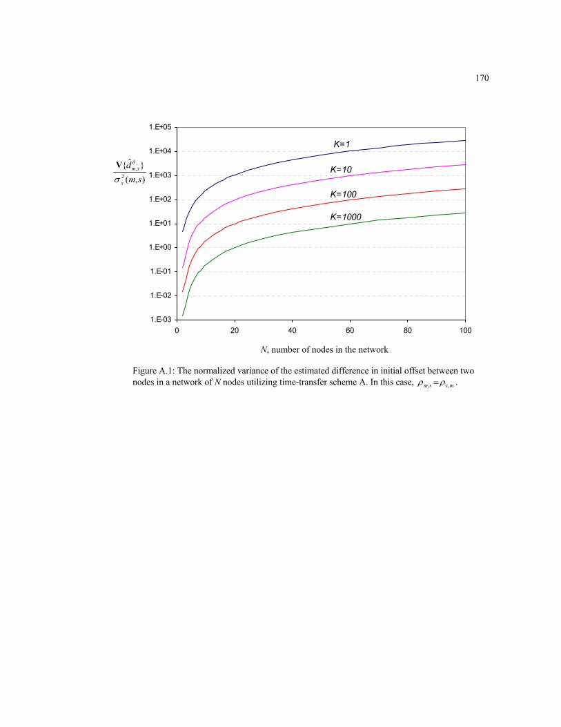
170
1.E-03
1.E-02
1.E-01
1.E+00
1.E+01
1.E+02
1.E+03
1.E+04
1.E+05
0 20 40 60 80 100
K=1
K=10
K=100
K=1000
Figure A.1: The normalized variance of the estimated difference in initial offset between two nodes in a network of N nodes utilizing time-transfer scheme A. In this case, mssm ,, ρρ = .
N, number of nodes in the network
),(ˆ
2,
smd
x
sm
σ
δV
171
APPENDIX B
VARIANCE OF TIMING ERRORS
The timing error between nodes m and s at time 't after time transfer is defined as
)()'(
)()(1
)()(
)()(1
)()(
)()(
sk
ssmk
mmsk
mk dtadtatt φφ −−′−++′=− ′′′ , (B.1)
where fTkt ′=′ .
B.1 Hierarchical Master-slave Timing Error
In this section, the timing errors after time synchronization using single-master-to-multiple-
slaves (SM) and hierarchical master-slaves (HM) time-transfer architectures are presented. In this
analysis, the variance of the timing error is defined as
2)()()1()1(1
)()(
)1()( 2
~~~ φσ+−′−+′=′sHM
sHM
sk'HMk dtadtat-t VV , s∀ , 1≠s , (B.2)
where )1(1a and )1(d are the drift and initial offset of the lead master node, and )(~ s
HMa , )(~ sHMd , )(
)'(~ s
kHMt are
the "settled" drift, initial offset and timing of node s after HM time transfer.
Let M be an ordered set whose elements are the node label of the roving masters. The
elements in the set are arranged according to the order at which node takes turn to be the roving
master. The element of M is denoted as )(qM where 1||,...,0 −= Mq and 1)0( =M is the lead master
node. If Q is the number of hops from lead master to roving master node m′ , from which node s
acquires its timing, then ')( mQ =M . From section 4.3, the settled initial offset at node s after HM
time-transfer is given by
∑≠
=−
− ++++=Q
sqq
qqqq
dsQsQ
dsHM dd
)(1
)(),1())(),1((
ˆ),()),((
ˆ)1()( ~~~
M
MMMM
MM ρερε , (B.3)
and the frame repetition rate )~( )(f
sHMTa= , is

172
∑≠
=
−++=Q
sqq
qqsQff
sHM LSLS
TaTa)(1
))(),1(()),(()1(1
)(~
M
MMMγγ εε , (B.4)
for 1≠s . The difference in initial offset, ),( smdδ between two nodes m and s is estimated by the
sample mean of 10
),( )( −=Kk
sm kϑ over K frames. From Chapter 3, this estimate is
KkdK
k
smsm /))((ˆ 1
0
),(),( ∑−
=−= ϑδ , (B.5)
and (3.23) states that ),(),(),(,
),(),( )ˆ())((~)( smsmLSf
smSTsm
smsm TaKkdk ϑδδ εγθρϑ +−⋅−+−−= , and )(kθ is
the characteristic function of the time-transfer scheme. For ji= , then
)6.(B.1))((1~
))((~1ˆ
1
0
),(1
0
),(,
),(
),(),(1
0,
),(),(
∑∑
∑−
=
−
=
−
=
−−++=
−⋅−++=
K
k
smST
K
k
smsm
sm
smsmK
kSTsm
smsm
KKk
Kd
KkdK
d
LS
LS
ϑγδ
ϑγδδ
εθερ
εεθρ
Therefore
.7)(B,~
ˆ~
),(ˆ,
)(
),()()(
smdsm
m
smssHM
d
ddd
ερδ
++=
+=
where
.1))((1 1),(
1
0
),(),(ˆ ∑∑
−+
=
−
=−−=
ST
STLS
KK
Kk
smK
kST
smsmd K
KkK ϑγ εθεε (B.8)
Similarly,
),()(1
)( ˆ~ smLSf
sf
sHM TaTa γ+= , (B.9)
where ),(),(),( ˆ smsmLS
smLSγεγγ −=− and
ˆ ),(),(),( smsmLS
smLSγεγγ VV =− . (B.10)
Substituting (B.3) and (B.4) into (B.2) and takes the expectation square, leads to

173
( ) ( )( ) ( )
)11.(B.222
~~~
)(~
222
~~~
)(~
~2
)~
(2~
)(~
22)~
()(~2
~~
~
2
)(1
))(),1((ˆ
))(),1(()),((ˆ
)),((
2
)(1
)(),1(),()()1(2)()1(
1
2
)(1
)'(1'
))'(),1'((ˆ
))(),1(()),((ˆ
)),((
2
)(1
)(),1(),()()1(2)()1(
1
)(1
)(),1())(),1((
ˆ)),((
ˆ
)(1
))(),1(()),((
2)1()(2)1()(2)1(1
)(
22)1()(22)1(1
)(
22)1()()1(1
)(
2)()(
)1()(
ΕΕ
VV
ΕΕ
VV
Ε
ΕVV
Ε
Ε
Ε
M
MMMMMM
M
MMM
M M
MMMMMM
M
MMM
M
MMMMM
M
MMM
φγγ
φγγ
γγ
φ
φ
φ
σεεεε
ρρ
σεεεε
ρρ
ρεεεε
σ
σ
σ
+′
⋅⋅⋅+′
⋅⋅⋅+
++−+′⋅−=
+′
⋅
⋅⋅+
′⋅⋅⋅+
++−+′⋅−=
′
⋅
++⋅
+⋅+
−++−+′⋅−=
++−+′⋅−=
+−+′⋅−=
−
∑
∑
∑ ∑
∑
∑∑
≠=
−−
≠=
−
≠=
≠=
−−
≠=
−
≠=
−−
≠=
−
′′
f
Q
sqq
qqd
f
sQd
sQ
Q
sqq
qqsQsHM
sHM
f
Q
sqq
Q
sqq
qqd
f
sQd
sQ
Q
sqq
qqsQsHM
sHM
f
Q
sqq
qqqq
dsQ
d
Q
sqq
qqsQ
sHM
sHM
sHM
sHM
sHM
sHM
sHM
skHMk
Tt
Tt
ddtaa
Tt
Tt
ddtaa
Tt
ddddtaa
ddtaa
ddtaa
tt
LSLS
LSLS
LSLS
Substituting (B.8) into (B.11) and from Appendix A,
01
),(),(1
),(),( =⋅=⋅ ∑∑−+
=
−+
=
ST
STLS
ST
STLS
KK
Kk
smsmSY
KK
Kk
smsmγγϑ εεεε ΕΕ . (B.12)
Therefore the cross-correlation term ),(ˆ
),( smd
smLS
εεγ ⋅Ε is
)13.(B.))((1
))((1
1
0
),(
1
0
),(),(),(ˆ
),(
V
ΕΕ
∑
∑−
=
−
=
−⋅=
−⋅=⋅
K
kST
sm
K
kST
smsmsmd
sm
KkK
KkK
LS
LSLSLS
θε
θεεεε
γ
γγγ
The variable STK is replaced with KQN )12( − for the time transfer from the roving master, denoted
by )(QM , to slave s . When timing is transferred from one roving master to another starting from the
lead master 1)0( =M to another roving master node denoted by )(qM , 0>q , then
)1()12( −−= qKNKST and (B.11) reduces to
174
( )
)14.(B.2
/2/2
~~
~
)(~~
2
)(1
))(),1(ˆ
))(),1()),(ˆ
)),(
2
)(1
)(),1(),(
)()1(2)()1(1
2)()(
)1()(
ΕΕ
VVΕ
M
M(MM(M(M(M
M
MMM
φ
γγ
σ
εεεε
ρρ
+
′⋅⋅⋅+′⋅⋅⋅+
++
−+′⋅−=−
∑
∑
≠=
−−
≠=
−
′′
Q
sqq
fqq
dqq
fsQ
dsQ
Q
sqq
qqsQ
sHM
sHM
skHMk
TtTt
ddtaatt
LSLS
At the end of the hierarchical master-slave time-transfer, i.e., ||M number of nodes have being the
roving master, then ||)12(' M⋅⋅−= KNt .
B.2 Mutually Synchronous Timing Error
In this section, the timing variance after mutually synchronous time-transfer is presented.
Note that instead of measuring the difference in timing between node s with respect to a lead master
node, the mean (average) of the sample variance of all nodes in the network after time transfer is of
interest. From (4.10) and (4.17),
),(1
1
)1,()1(1
)(~ sNN
n
nnff
sMU LSLS
TaTa γγ εε ++= ∑−
=
+ , (B.15a)
b).15(B,)~(
ˆ~
1
),(ˆ,
1,
)(,
1
),(,
)()(
∑∑
∑
≠=
≠=
≠=
⋅++⋅=
⋅+=
N
smm
smdsm
N
smm
smm
sm
N
smm
smsm
ssMU
d
ddd
εαρα
α δ
where ),(ˆ,
),(),( ~ˆ smdsm
smsm dd ερδδ ++= and ),(),(),(ˆ smsmLS
smLS LSγεγγ += . For the above quantities, the variance
across all nodes in the network is defined to be the sample variance. Then the mean of the variances
of )(~ sMUa , )(~ s
MUd and )()'(
~ skMUt across all nodes in the network are defined as
−
−= ∑ ∑
= =
N
s
N
s
sMU
sMUMU a
Na
Na
1
2
1
)()( ~1~1
1~ ΕV , (B.16a)
175
−
−= ∑ ∑
= =
N
s
N
s
sMU
sMUMU d
Nd
Nd
1
2
1
)()( ~1~1
1~
ΕV , (B.16b)
−
−= ∑ ∑
= =
N
s
N
s
skMU
skMUkMU t
Nt
Nt
1
2
1
)()'(
)()'()'(
~1~1
1~ ΕV , (B.16c)
where )(~ sMUa , )(~ s
MUd and )()'(
)()()()'(
~~~ sk
sMU
sMU
skMU dtat φ++′⋅= are the settled drift, initial offset and timing at
node s after time synchronization using a MU time-transfer architecture. The oscillator timing jitter
)()'(skφ is assumed to be i.i.d. with zero mean and variance 2
φσ .
To evaluate (B.16a), consider
a).17(B.1)(
11)(
21
)(1~1
12
1
1
12)1(1
1 1'
1
1
12
12
2)1(1
1 1'
1
1
)',()1,(2
1
),(2
1
1
1
)1,(2
1
)1(12
2
1
),(1
1
)1,()1(12
2
1
)(
VV
VV
Ε
ΕΕ
∑∑
∑∑ ∑∑
∑ ∑∑∑∑∑∑
∑ ∑∑
==
+
= = =
+
=
= = =
+
== =
+
=
= =
+
=
++=
++=
⋅+
+
+
⋅=
++⋅⋅=
⋅
N
s
(N,s)γ
N-
n
)(n,nγf
N
s
N
s
N-
n
)(n,nγ
N
s
(N,s)γf
N
s
N
s
N-
n
sNnnN
s
sNN
s
N-
n
nnN
sf
N
s
sNN-
n
nnf
N
sf
sMU
LSLS
LSLS
LSLSLSLS
LSLS
εN
εTa
εN
εN
Ta
TaN
TaN
TaN
γγγγ
γγ
εεεε
εε
Then
( ) ./1~1
22)(∑=
⋅=N
sf
N,sγMU Tε
Na
LSΕV (B.17b)
Similarly (B.16b) is evaluated as follows:
( )
( )
( ) a).18(B.~1~
11
~2~1~1
1
~~2~1~1
1
/~~
11
~
2
1
)(
1
2)(
2
1'
)'(2
1'
)'(
1
2)(
1 1'
)'()(2
1'
)'(2
2)(
1
2
1'
)'()(
Ε
Ε
Ε
ΕV
−
−=
−
+
−=
⋅−
+
−=
−
−=
∑∑
∑∑∑
∑ ∑∑
∑ ∑
==
===
= ==
= =
N
s
sMU
N
s
sMU
N
s
sMU
N
s
sMU
N
s
sMU
N
s
N
s
sMU
sMU
N
s
sMU
sMU
N
s
N
s
sMU
sMUMU
dN
dN
dN
dN
dN
ddN
dN
dN
NddN
d
176
Taking expectation on the squared of ∑−
N
s
sMUd
1
)( ,
( )
( ) ( ) b).18(B.~
~~
1
2)(ˆ
1
2,
2
1 .1,
)(,
2
1 ,1
),(ˆ,
2
1 .1,
)(,
2
1
)(
Ε
ΕΕ
∑ ∑∑ ∑
∑ ∑∑ ∑∑
=≠== ≠=
= ≠== ≠==
+
+⋅=
+
+⋅=
N
s
m,sd
N
smm
sm
N
s
N
smmsm
msm
N
s
N
smm
smdsm
N
s
N
smmsm
msm
N
s
sMU
εd
dd
αρα
εαρα
and from (B.15b),
( )
( ) c).18(B.)~(
)~(~
,1
2),(ˆ
2,
2
,1,
)(,
2
,1
),(ˆ,
2
,1,
)(,
2)(
Ε
ΕΕ
∑∑
∑∑
≠=
≠=
≠=
≠=
⋅+
+⋅=
⋅+
+⋅=
N
smm
smdsm
N
smm
smm
sm
N
smm
smdsm
N
smm
smm
smsMU
d
dd
εαρα
εαρα
Since ∑∑≠=
≠=
⋅++⋅=N
smm
smdsm
N
smm
smm
smsMU dd
1
),(ˆ,
1,
)(,
)( )~(~
εαρα , implies ∑≠=
⋅=N
sm,m
smdsm
sMUd
1
),(ˆ
2,
)( ~
εα VV and ),(ˆsm
dε has
zero mean. Therefore
( )
( )
( )
( ) d).18(B.~)1(
1
~1
1~
1
~)1(
1
~1
11~
2
1 .1,
)(,
1 1
2
.1,
)(,
)(
2
1 .1,
)(,
1 1
2
.1,
)(,
),(ˆ
,1
2,
V
VV
+⋅
−−
+⋅
−+=
+⋅
−⋅−
+⋅
−+=
∑ ∑
∑ ∑ ∑
∑ ∑
∑ ∑ ∑∑
= ≠=
= = ≠=
= ≠=
= = ≠=≠=
N
s
N
smmsm
msm
N
s
N
s
N
smmsm
msm
sMU
N
s
N
smmsm
msm
N
s
N
s
N
smmsm
msm
smd
N
smmsmMU
dNN
dN
dN
dNN
dNN
d
ρα
ρα
ρα
ραεα
To obtain the timing variance, we note that
)()'(
)()()()'(
~~~ sk
sMU
sMU
skMU dtat φ++′⋅= , (B.19a)
( ) ( ) ( ) ( ) )()'(
)()()'(
)(2)()'(
)()(2)(2)(2)()(
~2~2
~~2~~~ s
ksMU
sk
sMU
sk
sMU
sMU
sMU
sMU
skMU dtatdadtat φφφ ⋅⋅+⋅′⋅⋅++′⋅⋅⋅++′⋅=′ , (B.19 b)
177
c).19(B.22
2~~
)~~()
~~(~
1 1
)()'(
)'(
1 1
)()'(
)'(
1 1
)()'(2
1
)('
2
1
)(2
1
)(
1 1
)'()'(
)()()()'(
)()(2
1
)()'(
∑ ∑∑ ∑
∑ ∑∑∑∑
∑ ∑∑
= =′= =′
= =′===
= =′
′′
=
+′+
′+
+
+
′=
++′⋅++′=
N
s
N
s
sk
sMU
N
s
N
s
sk
sMU
N
s
N
s
sMU
sMU
N
s
sk
N
s
sMU
N
s
sMU
N
s
N
s
sk
sMU
sMU
sk
sMU
sMU
N
s
skMU
dta
tdadta
dtadtat
φφ
φ
φφ
Taking the expectation of (B.19b), we arrive at
( ) ( ) ( ) ( ) ( ) tdadtat sMU
sMU
sk
sMU
sMU
skMU ′⋅⋅⋅+++′⋅= )()(2)(
)'(
2)(22)(2)()'(
~~2~~~ ΕΕΕΕΕ φ , (B.19d)
and the timing variance at individual node after time transfer is
( ) ( ) ( ) ( ) 2)()'(
2)(22)()()'(
~~~ sk
sMU
sMU
skMU dtat φVVVV ++′⋅= . (B.19e)
From (B.15a),
( ) ( ) ( )
( ) ( ) ( ) a).20(B.//
/2
//~
22),(21
1
2)1,(2)1(1
21
1
),()1,(
22),(221
1
)1,(2)1(1
2)(
ΕΕ
Ε
ΕΕΕ
fsN
f
N
n
nn
f
N
n
sNnn
fsN
f
N
n
nnsMU
TTa
T
TTaa
LSLS
LSLS
LSLS
γγ
γγ
γγ
εε
εε
εε
++=
⋅+
+
+=
∑
∑
∑
−
=
+
−
=
+
−
=
+
The cross-correlation is evaluated as follows
b).20(B,
~~
,1
),(ˆ
),(,
1
1 ,1
),(ˆ
)1,(,
,1,,
)1(1
,1
)(,
)1(1
)()(
Ε
ΕΕ
∑
∑ ∑∑∑
≠=
−
=≠=
+
≠=
≠=
⋅⋅+
⋅⋅+⋅+⋅=⋅
N
smm
smd
sN
f
sm
N
n
N
smm
smd
nn
f
smN
smm
smsm
N
smm
msm
sMU
sMU
LS
LS
T
Tadada
εεα
εεα
ραα
γ
γ
and
c).20(B,)'(
~~
,1
)',(ˆ
),(,
1
1 ,1
),(ˆ
)1,(,
,1,,
)1(1
,1
)(,
)1(1
)()'(
Ε
ΕΕ
∑
∑ ∑∑∑
≠=
−
=≠=
+
≠=
≠=
−⋅⋅⋅+
⋅⋅+⋅+⋅=⋅
N
smm
smd
sN
f
sm
N
n
N
smm
smd
nn
f
smN
smm
smsm
N
smm
msm
sMU
sMU
ssT
Tadada
LS
LS
δεεα
εεα
ραα
γ
γ
where 1)'( =− ssδ if 'ss= , otherwise 0)'( =− ssδ . Moreover it can be shown that
178
),(ˆ
),(,
,1
),(ˆ
),(, sNd
sN
f
sNN
smm
smd
sN
f
smLSLS TT
εεα
εεα
γγ ⋅⋅=⋅⋅∑≠=
ΕΕ , (B.21a)
and
NsTT
ssd
ss
f
ssN
n
N
smm
smd
nn
f
smLSLS
<=<⋅⋅=⋅⋅ −−−−
=≠=
+∑ ∑ 1, ),1(ˆ
),1(,11
1 ,1
),(ˆ
)1,(, εεα
εεα
γγ ΕΕ . (B.21b)
The variance of the timing )~( 2)()'(
skMUtΕ at individual node s after MU time-transfer can be
evaluated by substituting (B.20a), (B.20b) and (B.20c) into (B.19c).
From (B.16c), the variance of the timing across all nodes in the network evaluates to
( ) .22)(B.
~~)1(
2
~~
12
~)(~~
2)()'(
1 1'
)()(
1
)()(2)'(
ΕΕ
ΕVVV
sk
N
s
N
s
sMU
sMU
N
s
sMU
sMUMUMUkMU
tdaNN
tdaN
dtat
φ+′⋅⋅−
−
′⋅⋅−
++′⋅=
∑∑
∑
= =
′
=
Substituting (B.20c) and (B.20d) into (B.22), equation (B.22) becomes
.23)(B,2~
)(~
1
)1(
2
1
2
~
)(~~
21
1
),(ˆ
),(,2
2),(ˆ
),(,
1
1
1 ,1
),(ˆ
)1,(,
,1,,
)1(1
,1
)(,
)1(1
),(ˆ
),(,
1
1
1 ,1
),(ˆ
)1,(,
,1,,
)1(1
,1
)(,
)1(1
2)'(
ΕVV
Ε
Ε
Ε
Ε
VVV
φγ
φγ
γ
γ
γ
σεεα
σεεα
εεα
ραα
εεα
εεα
ραα
+⋅⋅′⋅
++′⋅=
+
⋅⋅⋅+
⋅⋅+⋅+⋅
−⋅′⋅
−
⋅⋅+
⋅⋅+⋅+⋅
−′⋅
+
+′⋅=
∑
∑ ∑ ∑∑∑
∑ ∑ ∑∑∑
−
=
=
−
=≠=
+
≠=
≠=
=
−
=≠=
+
≠=
≠=
N
s
sNd
sN
f
sNMUMU
sNd
sN
f
sN
N
s
N
n
N
smm
smd
nn
f
smN
smm
smsm
N
smm
msm
sNd
sN
f
sN
N
s
N
n
N
smm
smd
nn
f
smN
smm
smsm
N
smm
msm
MUMUkMU
LS
LS
LS
LS
LS
TNtdta
TN
Tada
NNNt
T
Tada
Nt
dtat
where KQNKST )12( −= and mQ =)(M if nodes take turn to be the roving master in the natural
order. For MU, NKNk ⋅−= )12(' and NKTNt f)12(' −= .

179
APPENDIX C
SIMULATION RESULTS FOR HIERARCHICAL MASTER-SLAVE TIME-TRANSFER ARCHITECTURE
This appendix reports the simulation results obtained from simulating the hierarchical
master-slave time transfer architecture. Unless otherwise specified, the Monte Carlo simulations are
performed with the following simulation parameters:
1.) Number of nodes in network, 20=N .
2.) Nominal frame repetition rate, 310−=fT seconds.
3.) Approximate pulse width of UWB monocycle, 910067.0 −×=wσ seconds.
4.) Order of Gaussian derivative waveform, 8=n .
5.) Number of frames per slot, 1000=== rs KKK .
6.) Uplink and downlink index, ji= .
7.) Oscillator phase noise, 0=φσ .
8.) Path-loss exponent, 2=Lρ .
For the HM time-transfer architecture, simulations are performed with 5 and 19 roving
masters (including the lead master node). If nodes are aware of the signal propagation distances from
themselves to all other nodes in the network, i.e., nodes have complete knowledge of the network
topology, for 5 roving masters, the roving masters will be taken from the ordered set 1,8,12,4,2.
Similarly, for 19 roving masters, the nodes take turn to be the roving masters in the order
1,8,12,4,2,6,20,17,18,9,13,16,11,10,5,7,15,14,19.
The initial offset before time-transfer is,
=)(sd -0.15398521972836, 0.10680338700882, 0.17076648855833,
0.07034841669641, -0.07829529943844, -0.02252087387333,
0.05095257661642, 0.25459580650917, 0.23084002368445,

180
0.09858776012560, 0.11177512414205, 0.10387650348619,
0.28858078810527, 0.01802540503429, 0.10627836711161,
0.12694466466843, 0.00301192281376, 0.07173229031455,
0.27131321961697, 0.14643006878572 910−× secs.
The normalized drift before time transfer is,
=)(sη 1×10⁻⁶, 7×10⁻⁶, -4×10⁻⁶, 9×10⁻⁶, 5×10⁻⁶,
4×10⁻⁶, -8×10⁻⁶, -5×10⁻⁶, 2×10⁻⁶, -7×10⁻⁶,
8×10⁻⁶, 1×10⁻⁶, 7×10⁻⁶, -4×10⁻⁶, 8×10⁻⁶,
5×10⁻⁶, 7×10⁻⁶, 4×10⁻⁶, 3×10⁻⁶, -2×10⁻⁶ .
Therefore the drift of the nodes in the network before time-transfer is )()(1 1 ssa η+= .
1.5 15,1τ
1.5 20,1τ
0
5
10
15
20
0 5 10 15 20
1
2
3
4
5
6
7
8
9
10 11
12
13
1415
16
17
18
19
20
(met
ers)
1.5 17,1τ
(meters) NLOS signal propagation LOS signal propagation
Figure C.1: Network topology used for time transfer simulations. The simulations parameters are listed in the beginning of this Appendix. Node 1 is the lead master node.
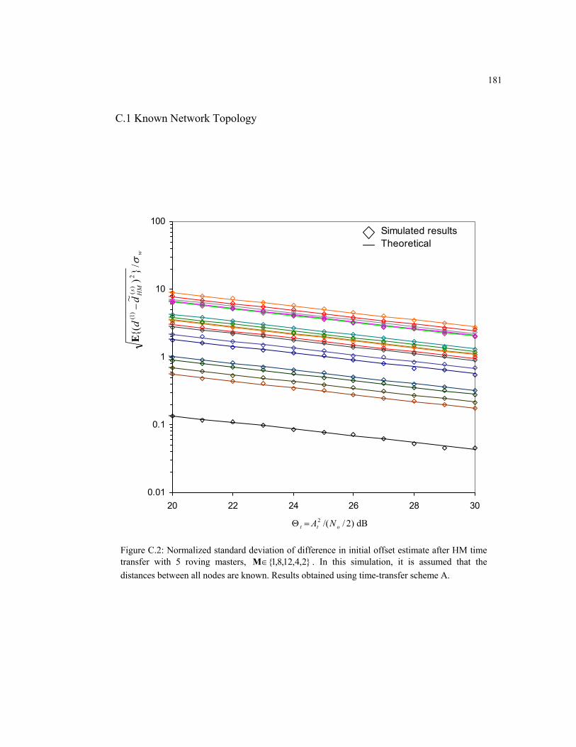
181
C.1 Known Network Topology
0.01
0.1
1
10
100
20 22 24 26 28 30
Simulated resultsTheoretical
)2//(2ott NA=Θ dB
Figure C.2: Normalized standard deviation of difference in initial offset estimate after HM time transfer with 5 roving masters, 2,4,12,8,1∈M . In this simulation, it is assumed that the distances between all nodes are known. Results obtained using time-transfer scheme A.
w
s HM
dd
σ/)
~(
2)
()1(−
Ε
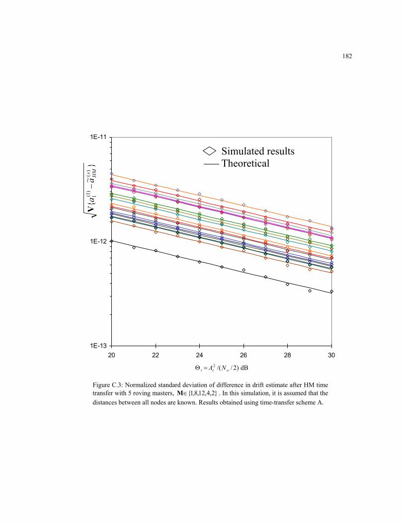
182
1E-13
1E-12
1E-11
20 22 24 26 28 30
)2//(2ott NA=Θ dB
Simulated results Theoretical
Figure C.3: Normalized standard deviation of difference in drift estimate after HM time transfer with 5 roving masters, 2,4,12,8,1∈M . In this simulation, it is assumed that the distances between all nodes are known. Results obtained using time-transfer scheme A.
~
)(
)1( 1s HM
aa
−V

183
0.01
0.1
1
10
100
1000
20 22 24 26 28 30
)2//(2ott NA=Θ dB
Simulated results Theoretical
Figure C.4: Normalized standard deviation of difference in initial offset estimate after HM time transfer with 19 roving masters. In this simulation, it is assumed that the distances between all nodes are known. The roving master are:
1,8,12,4,2,6,20,17,18,9,13,16,11,10,5,7,15,14,19. Results obtained using time-transfer scheme A.
w
s HM
dd
σ/)
~(
2)
()1(−
Ε

184
1E-13
1E-12
1E-11
20 22 24 26 28 30
)2//(2ott NA=Θ dB
Simulated results Theoretical
Figure C.5: Normalized standard deviation of difference in drift estimate after HM time transfer with 19 roving masters. In this simulation, it is assumed that the distances between all nodes are known. The y-axis is in log scale. Results obtained using time-transfer scheme A.
~
)(
)1( 1s HM
aa
−V
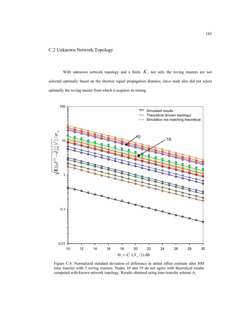
185
C.2 Unknown Network Topology
With unknown network topology and a finite K , not only the roving masters are not
selected optimally based on the shortest signal propagation distance, slave node also did not select
optimally the roving master from which it acquires its timing.
0.01
0.1
1
10
100
10 12 14 16 18 20 22 24 26 28 30
1910
Simulated resultsTheoretical (known topology)Simulation not matching theoretical
)2//(2ott NA=Θ dB
Figure C.6: Normalized standard deviation of difference in initial offset estimate after HM time transfer with 5 roving masters. Nodes 10 and 19 do not agree with theoretical results computed with known network topology. Results obtained using time-transfer scheme A.
w
s HM
dd
σ/)
~(
2)
()1(−
Ε

186
1E-13
1E-12
1E-11
1E-10
10 15 20 25 30
node 5
)2//(2ott NA=Θ dB
Simulated results Theoretical Simulation not matching theoretical
Figure C.7: Normalized standard deviation of difference in drift estimate after HM time transfer with 5 roving masters. Unlike variance of difference in initial offset, only node 5 deviates significantly from theoretical results computed with known network topology. Results obtained using time-transfer scheme A.
~
)(
)1( 1s HM
aa
−V
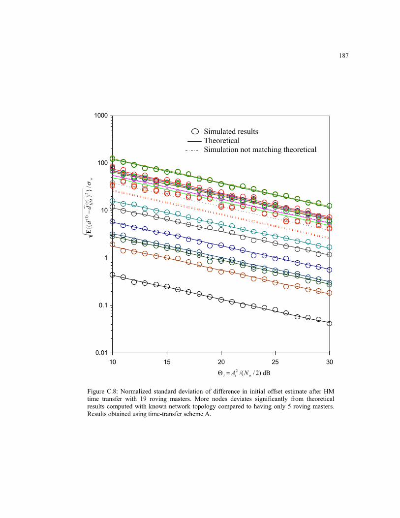
187
0.01
0.1
1
10
100
1000
10 15 20 25 30
)2//(2ott NA=Θ dB
Simulated results Theoretical Simulation not matching theoretical
Figure C.8: Normalized standard deviation of difference in initial offset estimate after HM time transfer with 19 roving masters. More nodes deviates significantly from theoretical results computed with known network topology compared to having only 5 roving masters. Results obtained using time-transfer scheme A.
w
s HM
dd
σ/)
~(
2)
()1(−
Ε
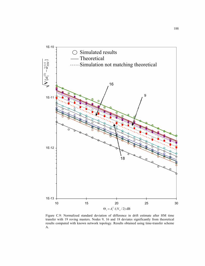
188
1E-13
1E-12
1E-11
1E-10
10 15 20 25 30
9
18
16
Simulated results Theoretical Simulation not matching theoretical
Figure C.9: Normalized standard deviation of difference in drift estimate after HM time transfer with 19 roving masters. Nodes 9, 16 and 18 deviates significantly from theoretical results computed with known network topology. Results obtained using time-transfer scheme A.
)2//(2ott NA=Θ dB
~
)(
)1( 1s HM
aa
−V

189
APPENDIX D
SIMULATION RESULTS FOR MUTUALLY SYNCHRONOUS TIME-TRANSFER ARCHITECTURE
0
2
4
6
8
10
12
14
16
1 2 3 4 5 6 7 8 9 10 11 12 13 14 15 16 17 18 19 20
10 dB
30 dB
Node label (s)
Simulated Theoretical
Figure D.1: Normalized standard deviation of the settled initial offset estimate for individual nodes in the network after MU (without NLoS propagation). The y-axis is in linear scale and the standard deviation is normalized with respect to wσ . The top most 'simulated' points are obtained at 10=Θ t dB, and in increment of 1 dB, the bottom most 'simulated' points are obtained at 30=Θ t dB. Results obtained using time-transfer scheme A.
w
sM
Ud
σ
~ )
(V

190
1.E-12
1.E-11
1.E-10
1 2 3 4 5 6 7 8 9 10 11 12 13 14 15 16 17 18 19 20
10 dB
30 dB
Node label (s)
Simulated Theoretical
Figure D.2: Standard deviation of the settled drift estimate after MU (without NLoS propagation) obtained from simulation and compared with theoretical analysis. The y-axis is in log scale. The top most 'simulated' points are obtained at 10=Θ t dB, and in increment of 1 dB, the bottom most 'simulated' points are obtained at 30=Θ t dB. Results obtained using time-transfer scheme A.
~ )
(s MU
aV

191
0
2
4
6
8
10
12
14
16
1 2 3 4 5 6 7 8 9 10 11 12 13 14 15 16 17 18 19 20
10 dB
30 dB
Simulated Theoretical
Node label (s)
Figure D.3: Normalized standard deviation of the settled initial offset estimate after MU for individual nodes in the network obtained from simulation and compared with theoretical analysis. In this simulation, NLoS propagation is introduced between nodes 1 and 15, 17 and 20 with receiver measurement error. The y-axis is in linear scale and the initial offset is normalized with respect to wσ . The top most 'simulated' points are obtained at 10=Θ t dB, and in increment of 1 dB, the bottom most 'simulated' points are obtained at 30=Θ t dB. Results obtained using time-transfer scheme A.
w
sM
Ud
σ
~ )
(V

192
0.0
0.5
1.0
1.5
2.0
2.5
3.0
3.5
4.0
4.5
5.0
1 2 3 4 5 6 7 8 9 10 11 12 13 14 15 16 17 18 19 20
20 dB
30 dB
Simulated Theoretical
Node label (s)
Figure D.4: Normalized standard deviation of the settled initial offset estimate after MU for individual nodes in the network obtained from simulation and compared with theoretical analysis. In this simulation, NLoS propagation is introduced between nodes 1 and 15, 17 and 20 with receiver measurement error. The y-axis is in linear scale and the initial offset is normalized with respect to wσ . The top most 'simulated' points are obtained at 10=Θ t dB, and in increment of 1 dB, the bottom most 'simulated' points are obtained at 30=Θ t dB. In order to verify the theoretical derivations, each network node is assumed to know the signal propagation distance from itself to all other nodes in the network. The simulated results agree well with the results obtained from the analytical equations. Results obtained using time-transfer scheme A.
w
sM
Ud
σ
~ )
(V
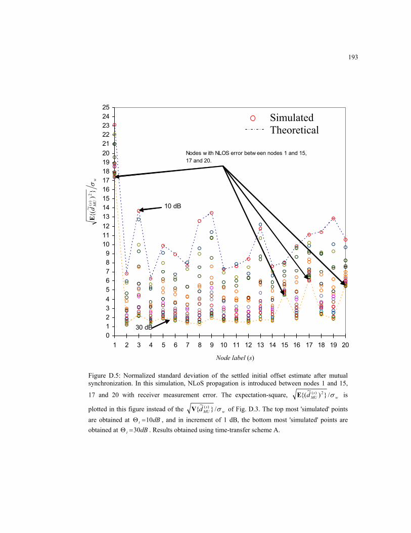
193
0123456789
10111213141516171819202122232425
1 2 3 4 5 6 7 8 9 10 11 12 13 14 15 16 17 18 19 20
10 dB
30 dB
Nodes w ith NLOS error betw een nodes 1 and 15, 17 and 20.
Simulated Theoretical
Node label (s)
Figure D.5: Normalized standard deviation of the settled initial offset estimate after mutual synchronization. In this simulation, NLoS propagation is introduced between nodes 1 and 15,
17 and 20 with receiver measurement error. The expectation-square, ws
MUd σ/)~
( 2)(Ε is
plotted in this figure instead of the ws
MUd σ/~
)(V of Fig. D.3. The top most 'simulated' points are obtained at dBt 10=Θ , and in increment of 1 dB, the bottom most 'simulated' points are obtained at dBt 30=Θ . Results obtained using time-transfer scheme A.
w
s MU
dσ
)
~(
2)
(Ε
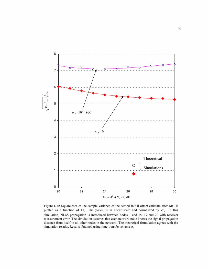
194
0
1
2
3
4
5
6
7
8
20 22 24 26 28 30
)2//(2ott NA=Θ dB
1110 −=φσ sec
Figure D.6: Square-root of the sample variance of the settled initial offset estimate after MU is plotted as a function of tΘ . The y-axis is in linear scale and normalized by wσ . In this simulation, NLoS propagation is introduced between nodes 1 and 15, 17 and 20 with receiver measurement error. The simulation assumes that each network node knows the signal propagation distance from itself to all other nodes in the network. The theoretical formulation agrees with the simulation results. Results obtained using time-transfer scheme A.
Theoretical Simulations
w
MU
dσ
~
V
0=φσ

195
1.E-13
1.E-12
1.E-11
10 15 20 25 30
~ MUaV
)2//(2ott NA=Θ dB
Simulated without NLoS Simulated with NLoS
Theoretical with NLoS
Figure D.7: Square-root of the sample variance of the settled drift estimate across all nodes in the network after MU is plotted as a function of tΘ . The y-axis is in log scale. As expected, there is no difference between propagations with LoS and without LoS. Results obtained using time-transfer scheme A.

196
APPENDIX E
SIMULATION RESULTS ON TIME-TRANSFER ERRORS USING TIME-TRANSFER SCHEME A
This appendix reports the timing errors of the SM, HM and MU time-transfer architectures
obtained from simulation. The simulation parameters are identical to those listed in Appendix C. The
network topology is shown in Fig. C.1.
100
120
140
160
180
200
220
24020 22 24 26 28 30
node 15
node 20
node 17
0
0.5
1
1.5
2
2.5
3
3.5
4
4.5
5
20 22 24 26 28 30
Simulated resultsTheoretical
)2//(2ott NA=Θ dB
Figure E.1: Normalized timing error standard deviation after SM time transfer, i.e., there is no roving of master nodes and fKTNt )12( −=′ . Time transfer from node 1 to nodes 15, 17 and 20 is impaired by receiver measurement error. In this simulation, in order to verify the theoretical derivations, each network node is assumed to know the signal propagation distance from itself to all other nodes in the network. Results obtained using time-transfer scheme A.
Nor
mal
ized
tim
ing
erro
r sta
ndar
d de
viat
ion
0=φσ
w
sk
SMk
tt
σ/)
~(
2)
()'
()1()'
(−
Ε

197
0
1
2
3
4
5
6
20 22 24 26 28 30
)2//(2ott NA=Θ dB
Simulated results Theoretical
Figure E.2: Normalized timing error standard deviation after HM time transfer with 5 roving masters. The roving master nodes are 2,4,12,8,1∈M . Here 5)12( ⋅−=′ fKTNt . In this simulation, in order to verify the theoretical derivations, each network node is assumed to know the signal propagation distance from itself to all other nodes in the network. The theoretical formulation agrees with the simulation results. Results obtained using time-transfer scheme A.
Nor
mal
ized
tim
ing
erro
r sta
ndar
d de
viat
ion
0=φσ
w
sk
HM
kt
tσ/
)~
(2
)(
)'(
)1()'
(−
Ε

198
0
5
10
15
20
25
30
35
20 22 24 26 28 30
)2//(2ott NA=Θ dB
Simulated results Theoretical
Figure E.3: Normalized timing error standard deviation after HM time transfer with 19 roving masters. The nodes take a turn as the roving master in the order: 1,8,12,4,2,6,20,17,18,9,13,16,11,10,5,7,15,14,19. And 19)12( ⋅−=′ fKTNt . In this simulation, in order to verify the theoretical derivations, each network node is assumed to know the signal propagation distance from itself to all other nodes in the network. The theoretical formulation agrees well with the simulation results. Results obtained using time-transfer scheme A.
Nor
mal
ized
tim
ing
erro
r sta
ndar
d de
viat
ion
0=φσ
w
sk
HM
kt
tσ/
)~
(2
)(
)'(
)1()'
(−
Ε

199
0
5
10
15
20
25
30
35
20 22 24 26 28 30
)2//(2ott NA=Θ dB
Figure E.4: Normalized timing sample variance across all nodes in the network after MU time transfer. Points labeled with 'known topology' refer to the simulation results when each network node is assumed to know the signal propagation distance from itself to all other nodes in the network. 'Unknown topology' refers otherwise. And 20)12( ⋅−=′ fKTNt for 20=N . Results obtained using time-transfer scheme A.
w
kMU
tσ
~
)'(
V Unknown Topology
Known Topology Theoretical
0=φσ
1110 −=φσ sec
Nor
mal
ized
tim
ing
stan
dard
dev
iatio
n ac
ross
all
node
s in
the
netw
ork
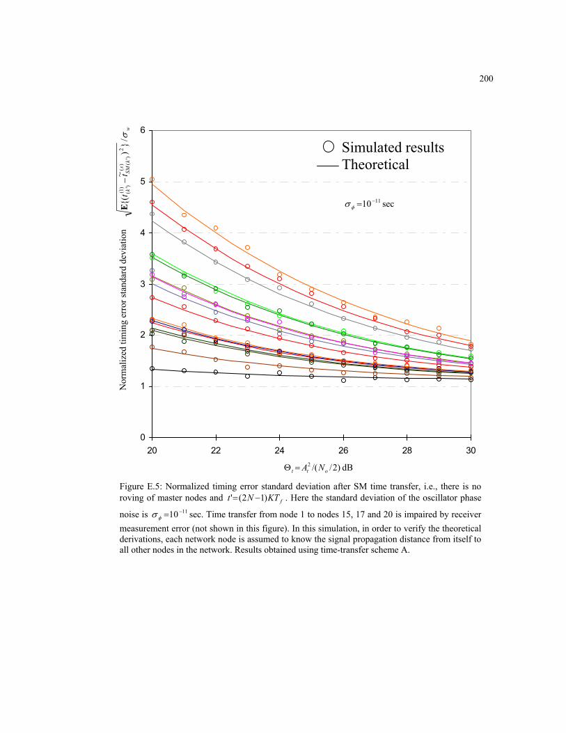
200
Figure E.5: Normalized timing error standard deviation after SM time transfer, i.e., there is no roving of master nodes and fKTNt )12(' −= . Here the standard deviation of the oscillator phase
noise is 1110 −=φσ sec. Time transfer from node 1 to nodes 15, 17 and 20 is impaired by receiver measurement error (not shown in this figure). In this simulation, in order to verify the theoretical derivations, each network node is assumed to know the signal propagation distance from itself to all other nodes in the network. Results obtained using time-transfer scheme A.
0
1
2
3
4
5
6
20 22 24 26 28 30
)2//(2ott NA=Θ dB
Simulated results Theoretical
Nor
mal
ized
tim
ing
erro
r sta
ndar
d de
viat
ion
1110 −=φσ sec
w
sk
SMk
tt
σ/)
~(
2)
()'
()1()'
(−
Ε
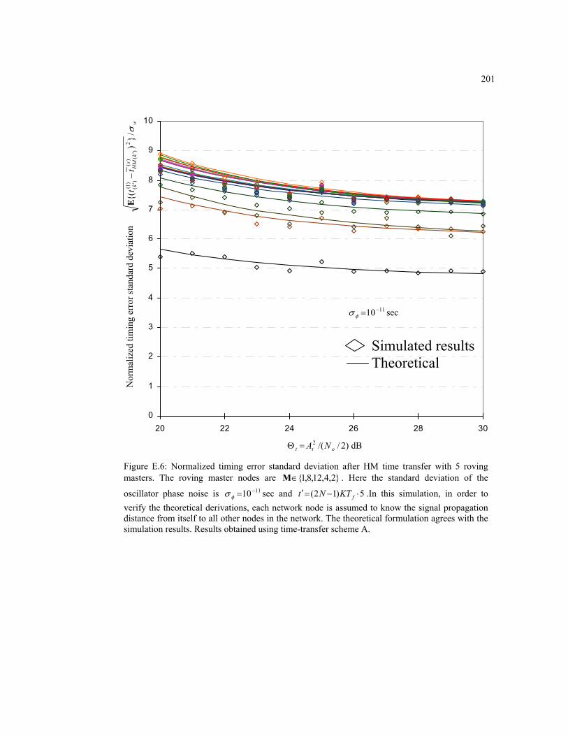
201
0
1
2
3
4
5
6
7
8
9
10
20 22 24 26 28 30
)2//(2ott NA=Θ dB
Simulated results Theoretical
Figure E.6: Normalized timing error standard deviation after HM time transfer with 5 roving masters. The roving master nodes are 2,4,12,8,1∈M . Here the standard deviation of the
oscillator phase noise is 1110 −=φσ sec and 5)12( ⋅−=′ fKTNt .In this simulation, in order to verify the theoretical derivations, each network node is assumed to know the signal propagation distance from itself to all other nodes in the network. The theoretical formulation agrees with the simulation results. Results obtained using time-transfer scheme A.
Nor
mal
ized
tim
ing
erro
r sta
ndar
d de
viat
ion
1110 −=φσ sec
w
sk
HM
kt
tσ/
)~
(2
)(
)'(
)1()'
(−
Ε
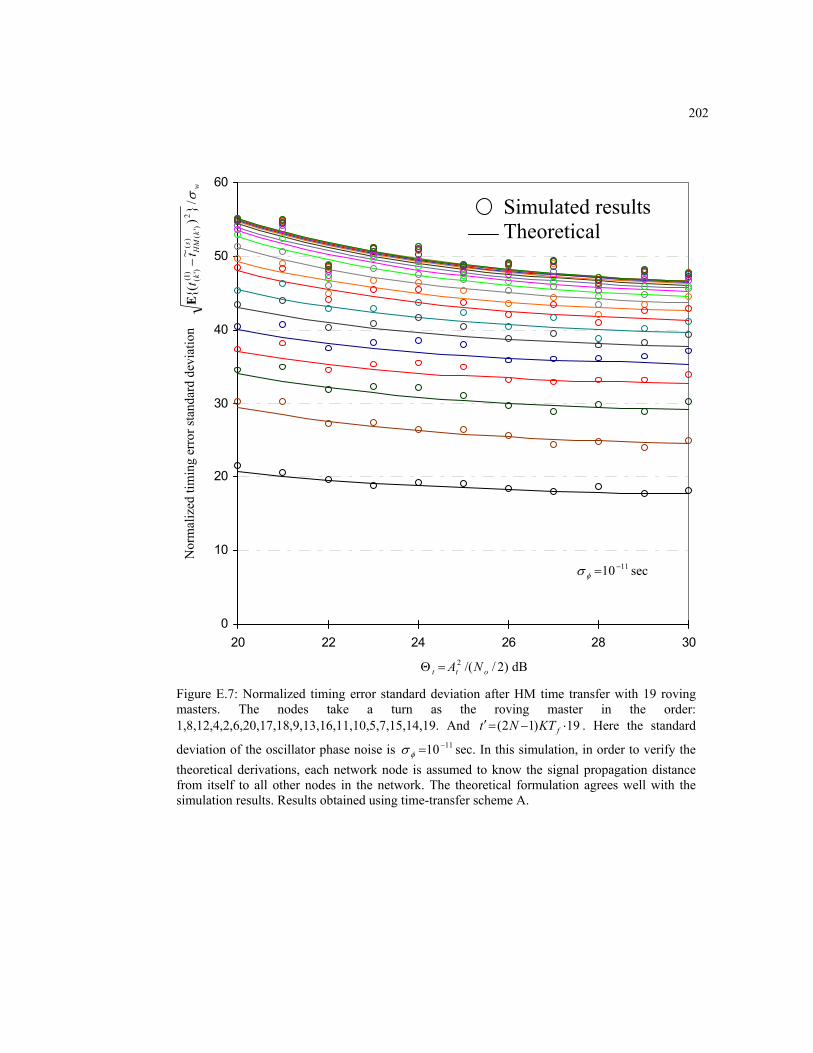
202
0
10
20
30
40
50
60
20 22 24 26 28 30
)2//(2ott NA=Θ dB
Simulated results Theoretical
Figure E.7: Normalized timing error standard deviation after HM time transfer with 19 roving masters. The nodes take a turn as the roving master in the order: 1,8,12,4,2,6,20,17,18,9,13,16,11,10,5,7,15,14,19. And 19)12( ⋅−=′ fKTNt . Here the standard
deviation of the oscillator phase noise is 1110 −=φσ sec. In this simulation, in order to verify the theoretical derivations, each network node is assumed to know the signal propagation distance from itself to all other nodes in the network. The theoretical formulation agrees well with the simulation results. Results obtained using time-transfer scheme A.
Nor
mal
ized
tim
ing
erro
r sta
ndar
d de
viat
ion
1110 −=φσ sec
w
sk
HM
kt
tσ/
)~
(2
)(
)'(
)1()'
(−
Ε
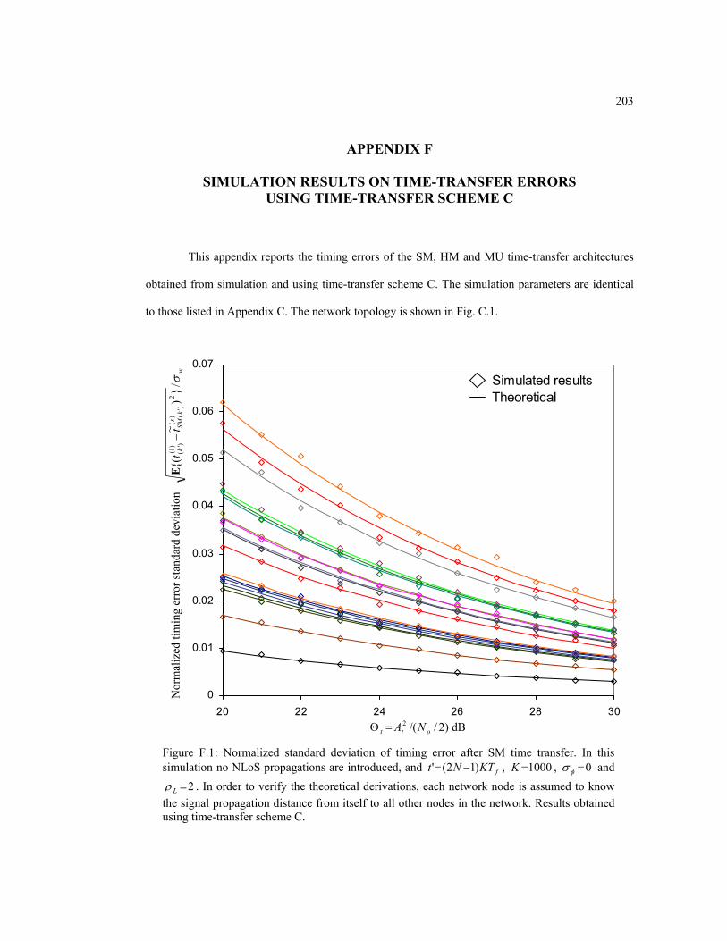
203
APPENDIX F
SIMULATION RESULTS ON TIME-TRANSFER ERRORS USING TIME-TRANSFER SCHEME C
This appendix reports the timing errors of the SM, HM and MU time-transfer architectures
obtained from simulation and using time-transfer scheme C. The simulation parameters are identical
to those listed in Appendix C. The network topology is shown in Fig. C.1.
0
0.01
0.02
0.03
0.04
0.05
0.06
0.07
20 22 24 26 28 30
Simulated resultsTheoretical
)2//(2ott NA=Θ dB
Figure F.1: Normalized standard deviation of timing error after SM time transfer. In this simulation no NLoS propagations are introduced, and fKTNt )12(' −= , 1000=K , 0=φσ and
2=Lρ . In order to verify the theoretical derivations, each network node is assumed to know the signal propagation distance from itself to all other nodes in the network. Results obtained using time-transfer scheme C.
Nor
mal
ized
tim
ing
erro
r sta
ndar
d de
viat
ion
wsk
SMk
tt
σ/)
~(
2)
()'
()1()'
(−
Ε

204
0.2
0.22
0.24
0.26
0.28
0.3
0.32
20 22 24 26 28 30
)2//(2ott NA=Θ dB
Simulated results Theoretical
Figure F.2: Normalized timing error standard deviation after HM time transfer with 5 roving masters. The roving master nodes are 2,4,12,8,1∈M . The network nodes have no knowledge of
the distances between themselves. Here 5)12( ⋅−=′ fKTNt , 1000=K , 1110 −=φσ sec and 2=Lρ and no NLoS propagation is introduced. Results obtained using time-transfer scheme C and 2100 Monte Carlo steps.
Nor
mal
ized
tim
ing
erro
r sta
ndar
d de
viat
ion
w
sk
HM
kt
tσ/
)~
(2
)(
)'(
)1()'
(−
Ε
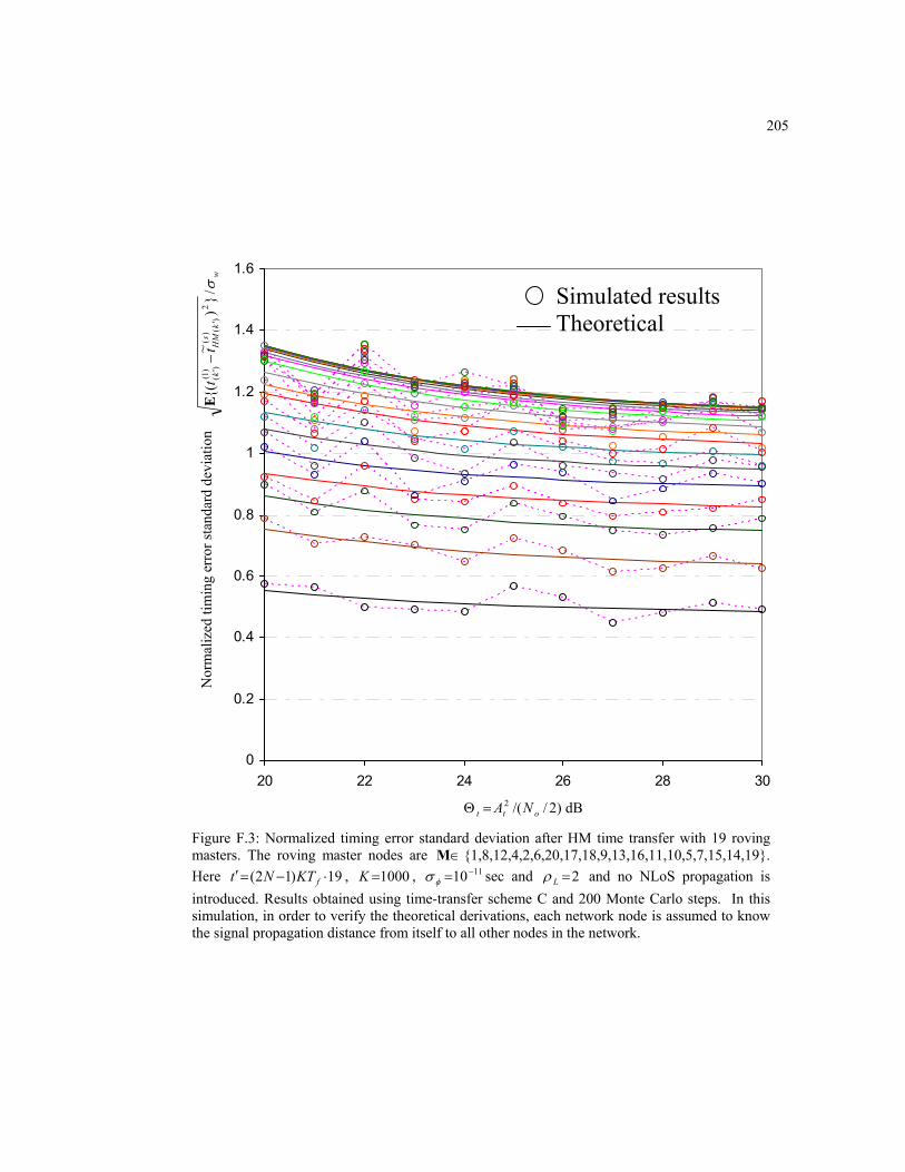
205
0
0.2
0.4
0.6
0.8
1
1.2
1.4
1.6
20 22 24 26 28 30
)2//(2ott NA=Θ dB
Simulated results Theoretical
Figure F.3: Normalized timing error standard deviation after HM time transfer with 19 roving masters. The roving master nodes are ∈M 1,8,12,4,2,6,20,17,18,9,13,16,11,10,5,7,15,14,19. Here 19)12( ⋅−=′ fKTNt , 1000=K , 1110 −=φσ sec and 2=Lρ and no NLoS propagation is introduced. Results obtained using time-transfer scheme C and 200 Monte Carlo steps. In this simulation, in order to verify the theoretical derivations, each network node is assumed to know the signal propagation distance from itself to all other nodes in the network.
Nor
mal
ized
tim
ing
erro
r sta
ndar
d de
viat
ion
wsk
HM
kt
tσ/
)~
(2
)(
)'(
)1()'
(−
Ε
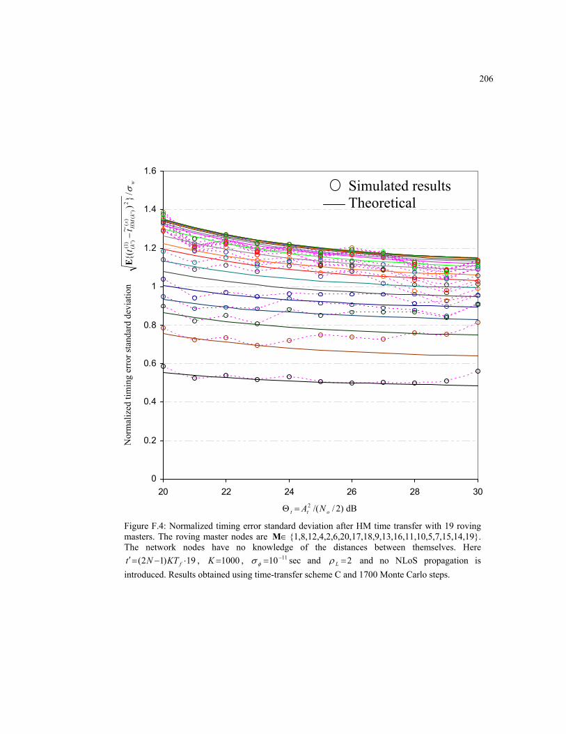
206
0
0.2
0.4
0.6
0.8
1
1.2
1.4
1.6
20 22 24 26 28 30
)2//(2ott NA=Θ dB
Simulated results Theoretical
Figure F.4: Normalized timing error standard deviation after HM time transfer with 19 roving masters. The roving master nodes are ∈M 1,8,12,4,2,6,20,17,18,9,13,16,11,10,5,7,15,14,19. The network nodes have no knowledge of the distances between themselves. Here
19)12( ⋅−=′ fKTNt , 1000=K , 1110 −=φσ sec and 2=Lρ and no NLoS propagation is introduced. Results obtained using time-transfer scheme C and 1700 Monte Carlo steps.
Nor
mal
ized
tim
ing
erro
r sta
ndar
d de
viat
ion
w
sk
HM
kt
tσ/
)~
(2
)(
)'(
)1()'
(−
Ε