switching transients analysis fundamentals - · pdf filean approved continuing education...
TRANSCRIPT

An Approved Continuing Education Provider
PDHonline Course E493 (5 PDH)
Switching Transients Analysis
Fundamentals
Velimir Lackovic, MScEE, P.E.
2015
PDH Online | PDH Center
5272 Meadow Estates Drive
Fairfax, VA 22030-6658
Phone & Fax: 703-988-0088
www.PDHonline.org
www.PDHcenter.com

www.PDHcenter.com PDHonline Course E493 www.PDHonline.org
©2015 Velimir Lackovic Page 2 of 38
Switching Transients Analysis Fundamentals
Velimir Lackovic, MScEE, P.E.
1. Introduction
An electrical transient occurs on a power system each time an abrupt circuit
change occurs. This circuit change is usually the result of a normal switching
operation, such as breaker opening or closing or simply turning a light switch on
or off. Bus transfer switching operations along with abnormal conditions, such as
inception and clearing of system faults, also cause transients.
The phenomena involved in power system transients can be classified into two
major categories:
- Interaction between magnetic and electrostatic energy stored in the
inductance and capacitance of the circuit, respectively
- Interaction between the mechanical energy stored in rotating machines
- Electrical energy stored in the inductance and capacitance of the circuit.
Most power system transients are oscillatory in nature and are characterized by
their transient period of oscillation. Despite the fact that these transient periods
are usually very short when compared with the power frequency of 50 Hz or 60
Hz, they are extremely important because at such times, the circuit components
and electrical equipment are subjected to the greatest stresses resulting from
abnormal transient voltages and currents. While over-voltages may result in
flashovers or insulation breakdown, overcurrent may damage power equipment
due to electromagnetic forces and excessive heat generation.
Flashovers usually cause temporary power outages due to tripping of the
protective devices, but insulation breakdown usually leads to permanent
equipment damage.
For this reason, a clear understanding of the circuit during transient periods is
essential in the formulation of steps required to minimize and prevent the
damaging effects of switching transients.
www.PDHcenter.com PDHonline Course E493 www.PDHonline.org
©2015 Velimir Lackovic Page 3 of 38
2. Circuit elements
All circuit elements, whether in utility systems, industrial plants, or commercial
buildings, possess resistance, R, inductance, L, and capacitance, C. Ohm’s law
defines the voltage across a time-invariant linear resistor as the product of the
current flowing through the resistor and its ohmic value. That is,
(1)
The other two elements, L and C, are characterized by their ability to store
energy. The term “inductance” refers to the property of an element to store
electromagnetic energy in the magnetic field. This energy storage is accomplished
by establishing a magnetic flux within the ferromagnetic material. For a linear
time-invariant inductor, the magnetic flux is defined as the product of the
inductance and the terminal current. Thus,
(2)
where φ(t) is the magnetic flux in webers (Wb), L is the inductance in henries
(H), and i(t) is the time-varying current in amperes (A). By Faraday’s law, the
voltage at the terminals of the inductor is the time derivative of the flux, namely,
(3)
Combining this relationship with Equation 2 gives the voltage-current relation of
a time-invariant linear inductor as
(4)
Finally, the term “capacitance” means the property of an element that stores
electrostatic energy. In a typical capacitance element, energy storage takes place
by accumulating charges between two surfaces that are separated by an insulating
material. The stored charge in a linear capacitor is related to the terminal voltage
by
(5)
www.PDHcenter.com PDHonline Course E493 www.PDHonline.org
©2015 Velimir Lackovic Page 4 of 38
where C is the capacitance in farads (F) when the units of q and v are in coulombs
(C) and volts (V), respectively. Since the electrical current flowing through a
particular point in a circuit is the time derivative of the electrical charge, Equation
5 can be differentiated with respect to time to yield a relationship between the
terminal current and the terminal voltage. Thus,
(6)
Under steady-state conditions, the energy stored in the elements swings between
the inductance and capacitance in the circuit at the power frequency. When there
is a sudden change in the circuit, such as a switching event, a redistribution of
energy takes place to accommodate the new condition. This redistribution of
energy cannot occur instantaneously for the following reasons:
- The electromagnetic energy stored in an inductor is .For a constant
inductance, a change in the magnetic energy requires a change in current.
But the change in current in an inductor is opposed by an emf of magnitude
. For the current to change instantaneously ( , an infinite
voltage is required. Since this is unrealizable in practice, the change in
energy in an inductor requires a finite time period.
- The electrostatic energy stored in a capacitor is given by and the
current-voltage relationship is given by . For a capacitor, an
instantaneous change in voltage requires an infinite current, which
cannot be achieved in practice. Therefore, the change in voltage in a
capacitor also requires finite time.
These two basic concepts, plus the recognition that the rate of energy produced
must be equal to the sum of the rate of energy dissipated and the rate of energy
stored at all times (principle of energy conservation) are basic to the
understanding and analysis of transients in power systems.

www.PDHcenter.com PDHonline Course E493 www.PDHonline.org
©2015 Velimir Lackovic Page 5 of 38
3. Analytical techniques
The classical method of treating transients consists of setting up and solving the
differential equation or equations, which must satisfy the system conditions at
every instant of time. The equations describing the response of such systems can
be formulated as linear time-invariant differential equations with constant
coefficients. The solution of these equations consists of two parts:
- The homogeneous solution, which describes the transient response of the
system, and
- The particular solution, which describes the steady-state response of the
system to the forcing function or stimulus.
Analytical solution of linear differential equations can also be obtained by the
Laplace transform method. This technique does not require the evaluation of the
constants of integration and is a powerful tool for complex circuits, where the
traditional method can be quite difficult.
4. Transient analysis based on the Laplace transform method
Although they do not represent the types of problems regularly encountered in
power systems, the transient analysis of the simple RL and RC circuits are useful
illustrative examples of how the Laplace transform method can be used for
solving circuit transient problems. Real-life circuits, however, are far more
complicated and often retain many circuit elements in series-parallel combination
even after simplification. These circuits will require several differential or
integro-differential equations to describe transient behaviour and must be solved
simultaneously to evaluate the response. To do this efficiently, the Laplace
transform method is often used.
5. LC transients
General types of circuits that are described by higher-order differential equations
are discussed. The double-energy transient, or LC circuit, is the first type of
circuit to be considered. In double-energy electric circuits, energy storage takes
place in the magnetic field of inductors and in the electric field of the capacitors.
In real circuits, the interchange of these two forms of energy may, under certain
www.PDHcenter.com PDHonline Course E493 www.PDHonline.org
©2015 Velimir Lackovic Page 6 of 38
conditions, produce electric oscillations. The theory of these oscillations is of
great importance in electric power systems.
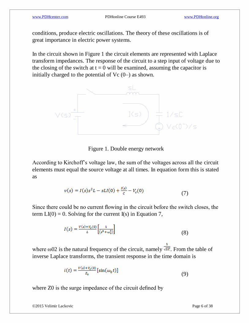
In the circuit shown in Figure 1 the circuit elements are represented with Laplace
transform impedances. The response of the circuit to a step input of voltage due to
the closing of the switch at t = 0 will be examined, assuming the capacitor is
initially charged to the potential of Vc (0–) as shown.
Figure 1. Double energy network
According to Kirchoff’s voltage law, the sum of the voltages across all the circuit
elements must equal the source voltage at all times. In equation form this is stated
as
(7)
Since there could be no current flowing in the circuit before the switch closes, the
term LI(0) = 0. Solving for the current I(s) in Equation 7,
(8)
where ω02 is the natural frequency of the circuit, namely . From the table of
inverse Laplace transforms, the transient response in the time domain is
(9)
where Z0 is the surge impedance of the circuit defined by
www.PDHcenter.com PDHonline Course E493 www.PDHonline.org
©2015 Velimir Lackovic Page 7 of 38
(10)
Clearly, the transient response indicates a sinusoidal current with a frequency
governed by the circuit parameters L and C only.
Another interesting feature about the time response of the current in the circuit is
that the magnitude of the current is inversely proportional to the surge impedance
of the circuit Z0, which is a function of the circuit parameters of L and C.
In power system analysis, we are often interested in the voltage across the
capacitor. Referring to Figure 1, the capacitor voltage is
(11)
where Vc(0) is the initial voltage of the capacitor. Solving for in the above
equation results in
(12)
But because the current I(s) is common to both elements L and C, we can
substitute Equation 12 into Equation 8 to obtain the voltage across the capacitor.
After rearranging the terms,
(13)
From the table of inverse Laplace transforms, the transient response is
(14)
The above equation is plotted in Figure 2 for various values of initial capacitor
voltage Vc(0).

www.PDHcenter.com PDHonline Course E493 www.PDHonline.org
©2015 Velimir Lackovic Page 8 of 38
Figure 2—Capacitor voltage for various initial voltages
Examination of these curves indicates that, without damping, the capacitor
voltage swings as far above the source voltage V as it starts below. In a real
circuit, however, this will not be the case, since circuit resistance will introduce
losses and will damp the oscillations. Treatment of the effects of resistance in the
analysis of circuits is presented next.
6. Damping
Nearly every practical electrical component has resistive losses (I2R losses). To
simplify the calculations and to ensure more conservative results, resistive losses
are usually neglected as a first attempt to a switching transient problem. Once the
behaviour of the circuit is understood, then system losses can be considered if
deemed necessary.
A parallel RLC circuit is depicted in Figure 3, in which the circuit elements are
represented by their Laplace transform admittances. Many practical transient
problems found in power systems can be reduced to this simple form and still
yield acceptable results. With a constant current source, I(s) and zero initial
conditions, the equation describing the current in the parallel branches is
(15)

www.PDHcenter.com PDHonline Course E493 www.PDHonline.org
©2015 Velimir Lackovic Page 9 of 38
Figure 3—Parallel RLC circuit
Solving for the voltage results in
(16)
Equation 16 can be written as
(17)
where r1 and r2 are the roots of the characteristic equation defined as follows:
(18)
At the natural resonant frequency ω0, the reactive power in the inductor is equal
to the power in the capacitor but opposite in sign. The source has to supply only
the true power PT required by the resistance in the circuit. The ratio between the
magnitude of the reactive power, PR, of either the inductance or the capacitance
at the resonant frequency, and the magnitude of true power, PT of the circuit, is
known as the quality factor of the circuit, or Q. Therefore, for the parallel circuit,
or or (19)
where B is the susceptance of either the inductor or capacitor, G is the
conductance, and V is the voltage across the element. But, since in a parallel

www.PDHcenter.com PDHonline Course E493 www.PDHonline.org
©2015 Velimir Lackovic Page 10 of 38
circuit the voltage is common to all elements, substituting ω0L for and R for
in Equation 19, the result is
(20)
Furthermore, since the natural frequency of the circuit is
(21)
then, substituting Equation 21 into Equation 20 yields
(22)
Rearranging Equation 18, we have
and (23)
Substituting Equation 22 into Equation 23, the result is
and (24)
Depending on the values of the circuit parameters, the quantity under the radical
in Equation 24 may be positive, zero, or negative.
For positive values, that is 4QP 2 < 1, the roots are real, negative, and unequal. In
this case, the inverse Laplace transform of Equation 17 is
(25)
where
(26)
www.PDHcenter.com PDHonline Course E493 www.PDHonline.org
©2015 Velimir Lackovic Page 11 of 38
is the damped natural angular frequency. Substituting 2sinh(ωDt) for the
exponential function, the result is
(27)
For the case where the quantity 4QP2 = 1, the roots are equal, negative, and real.
Therefore, the solution of Equation 25 is
(28)
Finally, when the quantity under the radical sign in Equation 4 is less than zero,
that is, 4QP2 > 1, the roots are unequal and complex. The solution in this case is
(29)
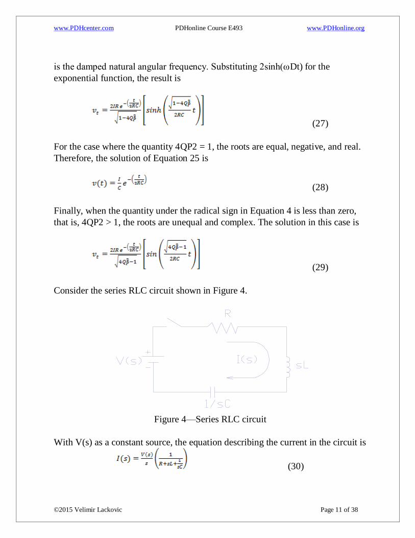
Consider the series RLC circuit shown in Figure 4.
Figure 4—Series RLC circuit
With V(s) as a constant source, the equation describing the current in the circuit is
(30)

www.PDHcenter.com PDHonline Course E493 www.PDHonline.org
©2015 Velimir Lackovic Page 12 of 38
Rearranging the terms results in
(31)
The expression inside the brackets is similar to the expression for the parallel
RLC circuit shown in Equation 16. The only difference is the coefficient of s.
Rewriting, as in Equation 17 gives
(32)
where r1 and r2 are the roots of the characteristic equation defined as
and (33)
Again, we define the quality factor of the series RLC circuit, Qs, as the ratio of
the magnitude of the reactive power of either the inductor or the capacitor at the
resonant frequency to the magnitude of the true power in the circuit. Stated in
equation form, results in
(34)
With the reactive power PR = I2X and the true power as PT = I2R, then
(35)
But since, in a series circuit, the current is common to all elements, then
(36)
where ω0L = X. Also, since then Equation 36 can be written as
www.PDHcenter.com PDHonline Course E493 www.PDHonline.org
©2015 Velimir Lackovic Page 13 of 38
or (37)
Note that the above expression is the ratio of the surge impedance to the
resistance in the circuit. This is the reciprocal of the expression developed for the
parallel RLC circuit and described by Equation 22. That is
(38)
Substituting Equation 37 into Equation 33 results in
and (39)
Above expressions have already been solved for the parallel RLC circuit. To
obtain the expression as a function of time, simply substitute Qs for QP and V/R
for IR and R/L for 1/RC in Equation 26 and Equation 28 and V/L for I/C and R/L
for 1/RC in Equation 29. Thus, when the quantity under the radical sign is less
than 1, namely, 4Qs 2 < 1, the result is
(40)
For the case where the quantity 4Qs 2 = 1, then the roots are equal, negative, and
real and the solution of Equation 39 is
(41)
Finally, when the quantity 4Qs 2 > 1, the roots are complex and unequal.
Therefore, the solution is
(42)
www.PDHcenter.com PDHonline Course E493 www.PDHonline.org
©2015 Velimir Lackovic Page 14 of 38
7. Normalized damping curves
The response of the parallel and series RLC circuits to a step input of current or
voltage, respectively, can be expressed as a family of normalized damping curves,
which can be used to estimate the response of simple switching transient circuits
to a step input of either voltage or current. To develop a family of normalized
damping curves, proceed as follows:
To per-unitize the solutions, we use the undamped response of a parallel LC
circuit as the starting point. Thus, for the voltage,
(43)
and, for the current,
(44)
The maximum voltage or current occurs when the angular displacement
ω0t = π /2. Thus,
and (45)
Setting the angular displacement ω0t = θ, the quantity in Equations 26
through 28 can be substituted with the expression .
Finally, dividing Equations 26 through 28 by the right side of the expression for
v(t) in Equation 45 produces a set of normalized curves for the voltage on the
parallel RLC circuit as a function of the dimensionless quantities QP and the
displacement θ.
Thus, for 4QP 2 <1,
(46)
www.PDHcenter.com PDHonline Course E493 www.PDHonline.org
©2015 Velimir Lackovic Page 15 of 38
And for 4QP 2 =1,
(47)
And for 4QP 2 >1 the result is
(48)
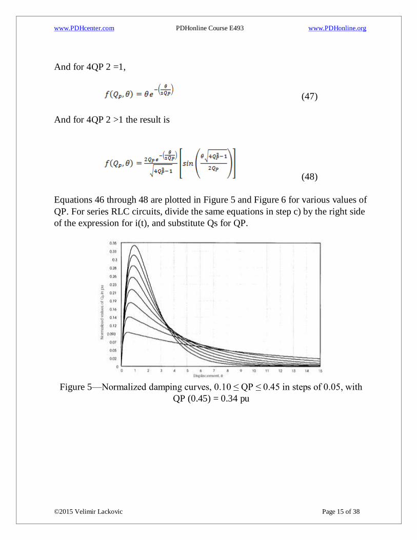
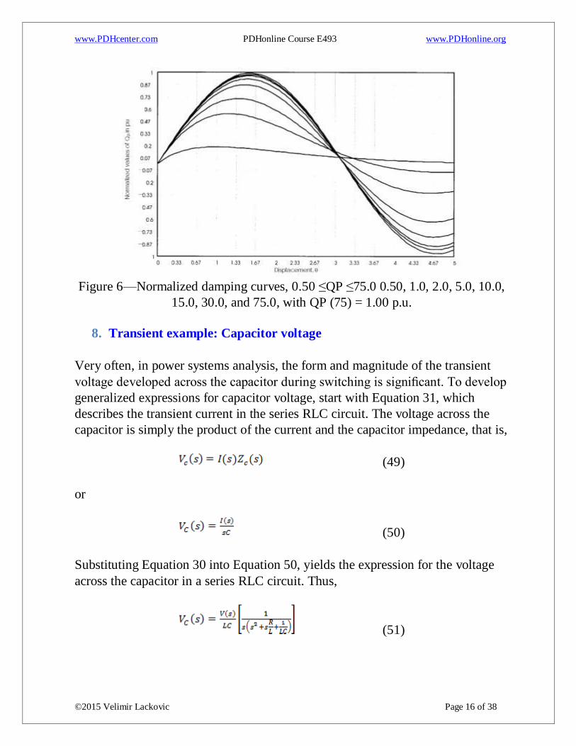
Equations 46 through 48 are plotted in Figure 5 and Figure 6 for various values of
QP. For series RLC circuits, divide the same equations in step c) by the right side
of the expression for i(t), and substitute Qs for QP.
Figure 5—Normalized damping curves, 0.10 ≤ QP ≤ 0.45 in steps of 0.05, with
QP (0.45) = 0.34 pu
www.PDHcenter.com PDHonline Course E493 www.PDHonline.org
©2015 Velimir Lackovic Page 16 of 38
Figure 6—Normalized damping curves, 0.50 ≤QP ≤75.0 0.50, 1.0, 2.0, 5.0, 10.0,
15.0, 30.0, and 75.0, with QP (75) = 1.00 p.u.
8. Transient example: Capacitor voltage
Very often, in power systems analysis, the form and magnitude of the transient
voltage developed across the capacitor during switching is significant. To develop
generalized expressions for capacitor voltage, start with Equation 31, which
describes the transient current in the series RLC circuit. The voltage across the
capacitor is simply the product of the current and the capacitor impedance, that is,
(49)
or
(50)
Substituting Equation 30 into Equation 50, yields the expression for the voltage
across the capacitor in a series RLC circuit. Thus,
(51)
www.PDHcenter.com PDHonline Course E493 www.PDHonline.org
©2015 Velimir Lackovic Page 17 of 38
Equation 51 is similar to the Equation 30, developed for the current, except that it
has an extra s term in the denominator. The expression can be rewritten as
follows:
(52)
where the roots of the equation are the same as those defined by Equation 39.
Again, the solution of Equation 52 will depend on the values of Qs.
Equation 14 shows the voltage across a capacitor due to a step input of voltage
when the resistance in the circuit is zero. For zero initial conditions, that is, no
charge in the capacitor, the last term in Equation 14 can be neglected. Then, the
maximum voltage occurs when ω0t= π. Therefore, the voltage is simply
(53)
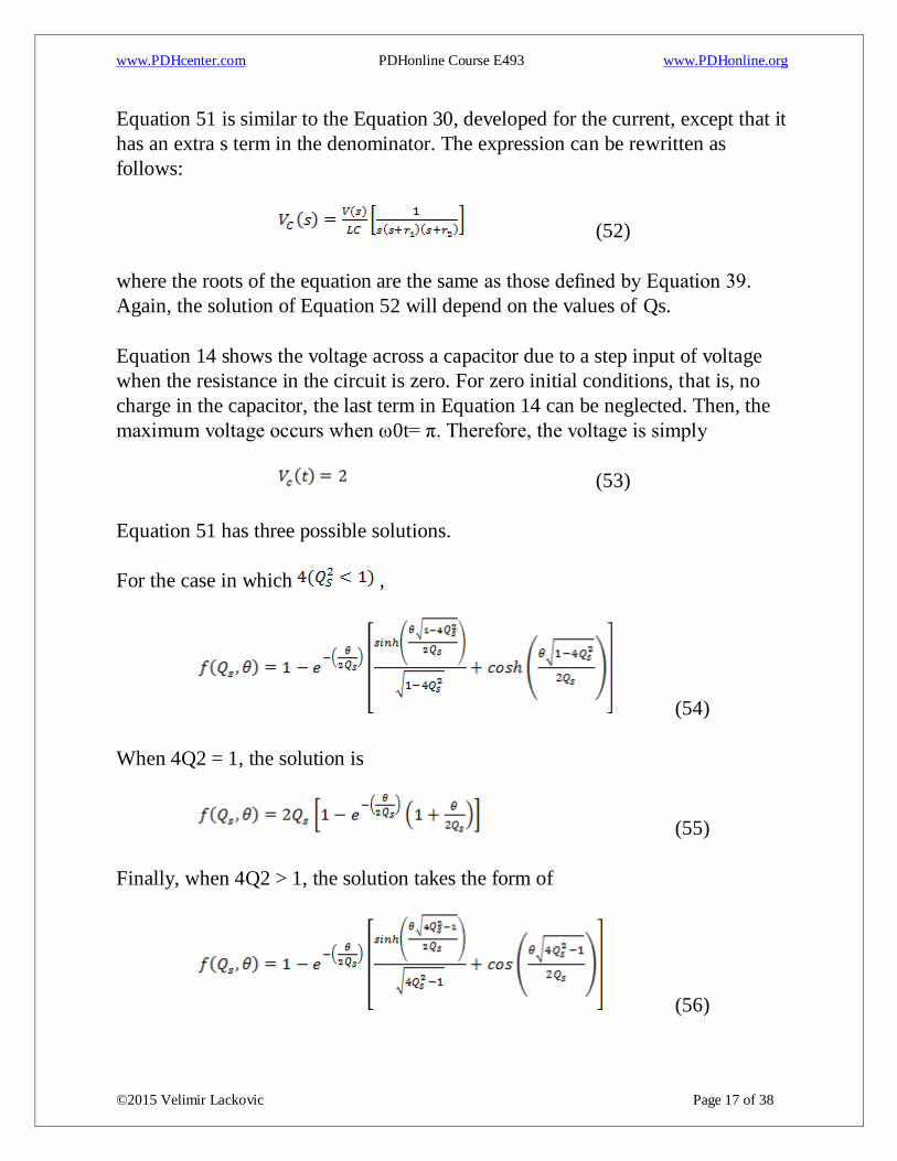
Equation 51 has three possible solutions.
For the case in which ,
(54)
When 4Q2 = 1, the solution is
(55)
Finally, when 4Q2 > 1, the solution takes the form of
(56)
www.PDHcenter.com PDHonline Course E493 www.PDHonline.org
©2015 Velimir Lackovic Page 18 of 38
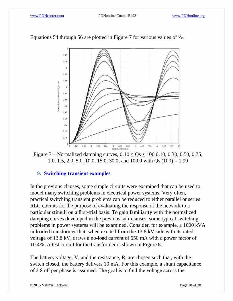
Equations 54 through 56 are plotted in Figure 7 for various values of .
Figure 7—Normalized damping curves, 0.10 ≤ Qs ≤ 100 0.10, 0.30, 0.50, 0.75,
1.0, 1.5, 2.0, 5.0, 10.0, 15.0, 30.0, and 100.0 with Qs (100) = 1.99
9. Switching transient examples
In the previous clauses, some simple circuits were examined that can be used to
model many switching problems in electrical power systems. Very often,
practical switching transient problems can be reduced to either parallel or series
RLC circuits for the purpose of evaluating the response of the network to a
particular stimuli on a first-trial basis. To gain familiarity with the normalized
damping curves developed in the previous sub-clauses, some typical switching
problems in power systems will be examined. Consider, for example, a 1000 kVA
unloaded transformer that, when excited from the 13.8 kV side with its rated
voltage of 13.8 kV, draws a no-load current of 650 mA with a power factor of
10.4%. A test circuit for the transformer is shown in Figure 8.
The battery voltage, V, and the resistance, R, are chosen such that, with the
switch closed, the battery delivers 10 mA. For this example, a shunt capacitance
of 2.8 nF per phase is assumed. The goal is to find the voltage across the

www.PDHcenter.com PDHonline Course E493 www.PDHonline.org
©2015 Velimir Lackovic Page 19 of 38
capacitance to ground, when the switch is suddenly opened and the flow of
current is interrupted.
Figure 8—Test setup of unloaded transformer
From the information provided, the no-load current of the transformer is
INL = 0.067794 – j0.64644 A
The magnetizing reactance XM and inductance LM per phase are, respectively
With a shunt capacitance of CSH = 2.8 nF, the shunt capacitive reactance is
Since XSH > XM, the effects of the shunt capacitive reactance at the power
frequency are negligible. The resistance RC is
Using delta-wye transformation impedance conversion, the circuit in Figure 8 can
be redrawn as shown in Figure 9.

www.PDHcenter.com PDHonline Course E493 www.PDHonline.org
©2015 Velimir Lackovic Page 20 of 38
Figure 9—Equivalent RLC circuit for unloaded transformer
In the Laplace transform notation, the equation describing the circuit at t = 0+ is
Assuming that dc steady-state was obtained before the switch opened, the term
CVc (0–) = 0 and the initial current in the inductor at t = 0+ is IL (0–) = 10 mA.
Solving for Vc(s) and after rearranging the terms, gives
The time-response solution for this expression has already been obtained and,
depending on the values of the circuit parameters, is shown in Equations 26, 27,
and 28. The values for R, L, and C could be inserted into one of those equations
to obtain the capacitor voltage for this problem. But this has also been done
through the normalized damping curves shown in Figure 5. Therefore, the
answers for this particular problem are obtained as follows:
The surge impedance of the circuit is

www.PDHcenter.com PDHonline Course E493 www.PDHonline.org
©2015 Velimir Lackovic Page 21 of 38
Without damping, the peak transient voltage would be
But since there is damping, the quality factor of the parallel circuit QP is
From the curves shown in Figure 5 and with QP ≈ 1.0, the maximum per unit
voltage is 0.57. Therefore, from previous step, the maximum voltage developed
across the capacitor is
The maximum peak occurs at approximately θ = 1.2 radians. Since ω 0t = θ and
or
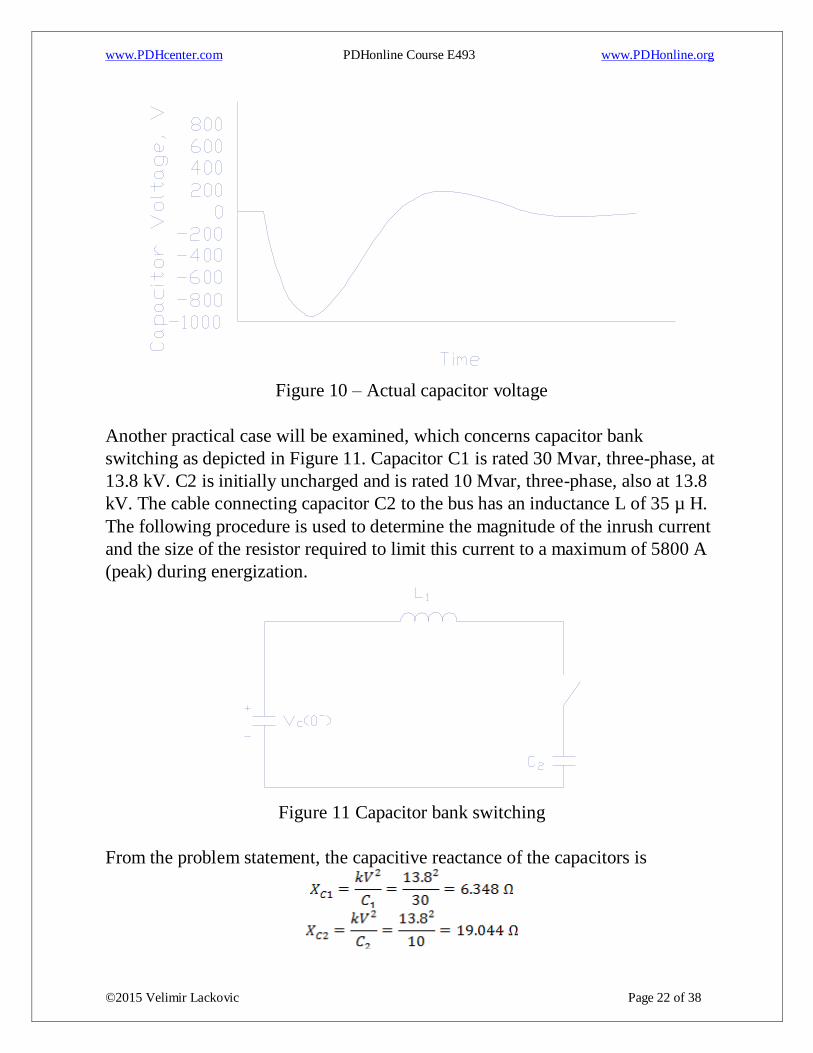
Figure 10 depicts the actual voltage across the capacitance to ground as calculated
by a computer program.
www.PDHcenter.com PDHonline Course E493 www.PDHonline.org
©2015 Velimir Lackovic Page 22 of 38
Figure 10 – Actual capacitor voltage
Another practical case will be examined, which concerns capacitor bank
switching as depicted in Figure 11. Capacitor C1 is rated 30 Mvar, three-phase, at
13.8 kV. C2 is initially uncharged and is rated 10 Mvar, three-phase, also at 13.8
kV. The cable connecting capacitor C2 to the bus has an inductance L of 35 µ H.
The following procedure is used to determine the magnitude of the inrush current
and the size of the resistor required to limit this current to a maximum of 5800 A
(peak) during energization.
Figure 11 Capacitor bank switching
From the problem statement, the capacitive reactance of the capacitors is

www.PDHcenter.com PDHonline Course E493 www.PDHonline.org
©2015 Velimir Lackovic Page 23 of 38
and the capacitance is
Assuming worst-case conditions, that is, C1 charged to peak system voltage or
and with a surge impedance of
Then, with no damping, the inrush current would be
Redrawing the circuit of Figure 11 to show the necessary addition of a resistor to
limit the inrush current yields the circuit as shown in Figure 12.
Figure 12—Equivalent circuit for capacitor switching with pre-insertion resistor
The problem requires that the inrush current should not exceed 5800 A. This
represents a per-unit value of

www.PDHcenter.com PDHonline Course E493 www.PDHonline.org
©2015 Velimir Lackovic Page 24 of 38
Referring to Figure 5, since the current problem concerns a series circuit, Qs
replaces QP. With a per-unit value requirement of 0.30 (vertical axis), Figure 5
shows that a QP = 0.30 will reduce the current to 5800 (19467 × 0.30) A or less.
Now, since
and
then
Therefore, to limit the inrush current to 5800 A a 1.9 Ω resistor must be placed in
series with capacitor C2 as shown in Figure 12.
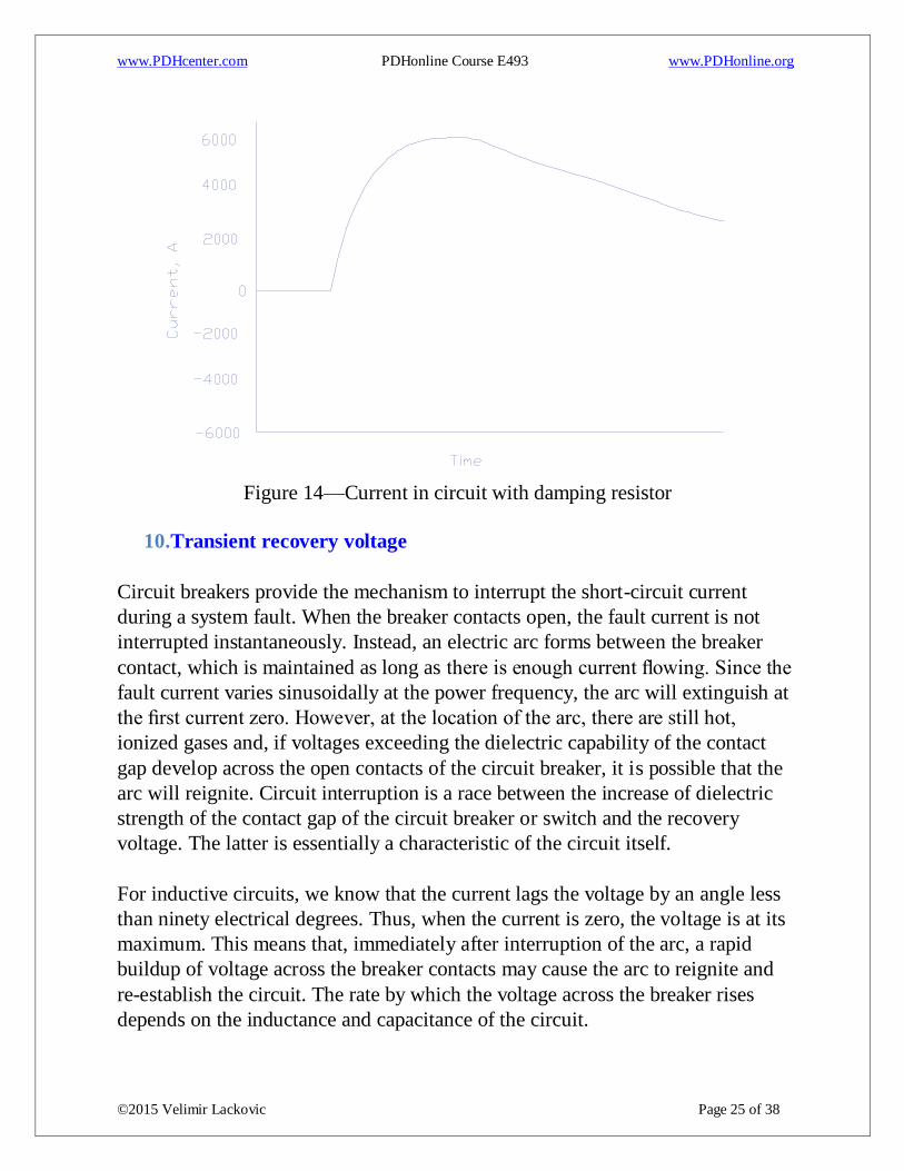
The results of a computer simulation are depicted in Figure 13 and Figure 14.
While Figure 13 shows the current without the pre-insertion resistor, Figure 14
reflects the current with the 1.9 Ω resistor.
Figure 13—Current in circuit without damping resistor
www.PDHcenter.com PDHonline Course E493 www.PDHonline.org
©2015 Velimir Lackovic Page 25 of 38
Figure 14—Current in circuit with damping resistor
10. Transient recovery voltage
Circuit breakers provide the mechanism to interrupt the short-circuit current
during a system fault. When the breaker contacts open, the fault current is not
interrupted instantaneously. Instead, an electric arc forms between the breaker
contact, which is maintained as long as there is enough current flowing. Since the
fault current varies sinusoidally at the power frequency, the arc will extinguish at
the first current zero. However, at the location of the arc, there are still hot,
ionized gases and, if voltages exceeding the dielectric capability of the contact
gap develop across the open contacts of the circuit breaker, it is possible that the
arc will reignite. Circuit interruption is a race between the increase of dielectric
strength of the contact gap of the circuit breaker or switch and the recovery
voltage. The latter is essentially a characteristic of the circuit itself.
For inductive circuits, we know that the current lags the voltage by an angle less
than ninety electrical degrees. Thus, when the current is zero, the voltage is at its
maximum. This means that, immediately after interruption of the arc, a rapid
buildup of voltage across the breaker contacts may cause the arc to reignite and
re-establish the circuit. The rate by which the voltage across the breaker rises
depends on the inductance and capacitance of the circuit.
www.PDHcenter.com PDHonline Course E493 www.PDHonline.org
©2015 Velimir Lackovic Page 26 of 38
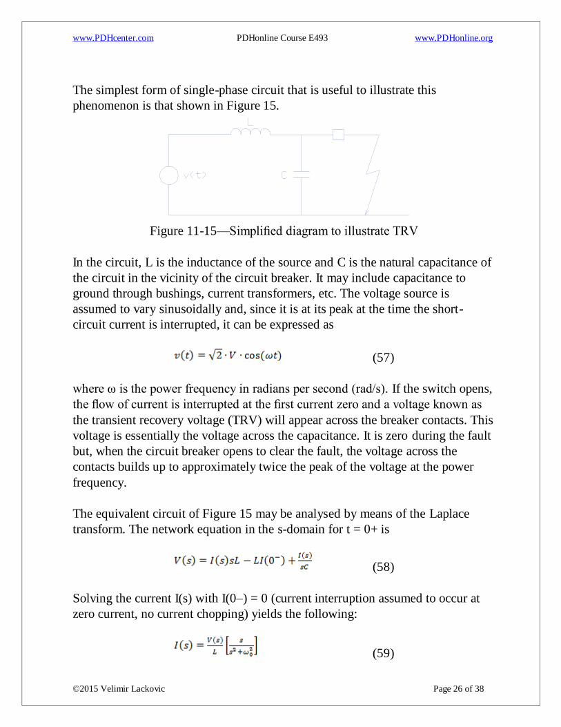
The simplest form of single-phase circuit that is useful to illustrate this
phenomenon is that shown in Figure 15.
Figure 11-15—Simplified diagram to illustrate TRV
In the circuit, L is the inductance of the source and C is the natural capacitance of
the circuit in the vicinity of the circuit breaker. It may include capacitance to
ground through bushings, current transformers, etc. The voltage source is
assumed to vary sinusoidally and, since it is at its peak at the time the short-
circuit current is interrupted, it can be expressed as
(57)
where ω is the power frequency in radians per second (rad/s). If the switch opens,
the flow of current is interrupted at the first current zero and a voltage known as
the transient recovery voltage (TRV) will appear across the breaker contacts. This
voltage is essentially the voltage across the capacitance. It is zero during the fault
but, when the circuit breaker opens to clear the fault, the voltage across the
contacts builds up to approximately twice the peak of the voltage at the power
frequency.
The equivalent circuit of Figure 15 may be analysed by means of the Laplace
transform. The network equation in the s-domain for t = 0+ is
(58)
Solving the current I(s) with I(0–) = 0 (current interruption assumed to occur at
zero current, no current chopping) yields the following:
(59)
www.PDHcenter.com PDHonline Course E493 www.PDHonline.org
©2015 Velimir Lackovic Page 27 of 38
Substituting sCVc(s) for I(s), the result is
(60)
The Laplace transform of the driving function described by Equation 57 is
(61)
Combining Equations 60 and 61, the recovery voltage or the voltage across the
capacitor is
(62)
From the table of the inverse Laplace transforms, the transient response is
(63)
The events before and after the fault are depicted in Figure 16 with damping.
However, without damping as described by Equation 63, the recovery voltage
reaches a maximum of twice the source voltage (the peak occurs at one half cycle
of the natural frequency, after the switch is opened). This is true when the natural
frequency is high as compared with the fundamental frequency and when losses
are insignificant. Losses (damping) will reduce the maximum value of Vc, as
shown in Figure 16.

www.PDHcenter.com PDHonline Course E493 www.PDHonline.org
©2015 Velimir Lackovic Page 28 of 38
Figure 16—Transient recovery voltage
Upon interruption of the fault current by the circuit breaker, the source attempts
to charge the capacitor voltage to the potential of the supply. As a matter of fact,
without damping, the capacitor voltage will overshoot the supply voltage by the
same amount as it started below. If the natural frequency of the circuit is high (L
and C very small), the voltage across the breaker contacts will rise very rapidly. If
this rate-of-rise exceeds the dielectric strength of the medium between the
contacts, the breaker will not be able to sustain the voltage and re-ignition will
occur.
11. Switching transient studies
Unlike classical power system studies, i.e., short circuit, load flow, etc., switching
transient studies are conducted less frequently in industrial power distribution
systems. Capacitor and harmonic filter bank switching in industrial and utility
systems account for most of such investigations, to assist in the resolution of
certain transient behavioural questions in conjunction with the application or
failure of a particular piece of equipment.
Two basic approaches present themselves in the determination and prediction of
switching transient duties in electrical equipment: direct transient measurements
(to be discussed later in this chapter) and computer modelling. The latter can be
divided into transient network analyser (TNA) and digital computer modelling.

www.PDHcenter.com PDHonline Course E493 www.PDHonline.org
©2015 Velimir Lackovic Page 29 of 38
In fact, experienced transient analysts use known circuit-response patterns, based
on a few basic fundamentals, to assess the general transient behaviour of a
particular circuit and to judge the validity of more complex switching transient
results. Indeed, simple configurations consisting of linear circuit elements can be
processed by hand as a first approximation. Beyond these relatively simple
arrangements, the economics and effective determination of electrical power
system transients require the utilization of TNAs or digital computer programs.
12. Switching transient study objectives
The basic objectives of switching transient investigations are to identify and
quantify transient duties that may arise in a system as a result of intentional or
unintentional switching events, and to prescribe economical corrective measures
whenever deemed necessary. The results of a switching transient study can affect
the operating procedures as well as the equipment in the system. The following
include some specific broad objectives, one or more of which are included in a
given study:
- Identify the nature of transient duties that can occur for any realistic
switching operation. This includes determining the magnitude, duration, and
frequency of the oscillations.
- Determine if abnormal transient duties are likely to be imposed on
equipment by the inception and/or removal of faults.
- Recommend corrective measures to mitigate transient over-voltages and/or
over-currents. This may include solutions such as resistor pre-insertion, tuning
reactors, appropriate system grounding, and application of surge arresters and
surge-protective capacitors.
- Recommend alternative operating procedures, if necessary, to minimize
transient duties.
- Document the study results on a case-by-case basis in readily
understandable form for those responsible for design and operation. Such
documentation usually includes reproduction of waveshape displays and
interpretation of, at least, the limiting cases.
www.PDHcenter.com PDHonline Course E493 www.PDHonline.org
©2015 Velimir Lackovic Page 30 of 38
13. Control of switching transients
The philosophy of mitigation and control of switching transients revolves around
the following:
- Minimizing the number and severity of the switching events
- Limitation of the rate of exchange of energy that prevails among system
elements during the transient period
- Extraction of energy
- Shifting the resonant points to avoid amplification of particular offensive
frequencies
- Provision of energy reservoirs to contain released or trapped energy within
safe limits of current and voltage
- Provision of discharge paths for high-frequency currents resulting from
switching
In practice, this is usually accomplished through one or more of the following
methods:
- Temporary insertion of resistance between circuit elements; for example,
the insertion of resistors in circuit breakers
- Synchronized closing control for vacuum and SF6 breakers and switches
- Inrush control reactors
- Damping resistors in filter and surge protective circuits
- Tuning reactors
- Surge capacitors
- Filters
- Surge arresters
- Necessary switching only, with properly maintained switching devices
- Proper switching sequences
14. Transient network analyzer (TNA)
Through the years, a small number of TNAs have been built for the purpose of
performing transient analysis in power systems. A typical TNA is made of scaled-
down power system component models, which are interconnected in such a way
as to represent the actual system under study. The inductive, capacitive, and
resistive characteristics of the various power system components are modelled
www.PDHcenter.com PDHonline Course E493 www.PDHonline.org
©2015 Velimir Lackovic Page 31 of 38
with inductors, capacitors, and resistors in the analyser. These have the same
oersted ohmic value as the actual components of the system at the power
frequency. The analyser generally operates in the range of 10–100 Vrms line-to-
neutral, which represents 1.0 per-unit voltage on the actual system.
The model approach of the TNA finds its virtue in the relative ease with which
individual components can duplicate their actual power system counterparts as
compared with the difficulty of accurately representing combinations of nonlinear
interconnected elements in a digital solution. Furthermore, the switching
operation that produces the transients is under the direct control of the operator,
and the circuit can easily be changed to show the effect of any parameter
variation. TNA simulation is also faster than digital simulation especially for
larger systems with many nonlinear elements to model.
15. Modelling techniques
Typical hardware used in a TNA to model the actual system components will be
described now. However, it should be fully recognized that any specific set of
components can be modelled in more than one way, and considerable judgment
on the part of the TNA staff is necessary to select the optimum model for a given
situation. Also, it should be recognized that, while there is a great similarity
among the components of the various TNAs in existence today, there are also
unique hardware approaches to any given system. The following is a general
description of some of the hardware models.
- Transmission lines are modelled basically as a four-wire system, with three
wires associated with the phase conductors and the fourth wire encompassing the
effects of shield wire and earth return.
- Circuit breakers consist of a number of independent mercury-wetted relay
contacts or solid-state electronic circuitry. The instant of both closing and
opening of each individual switch can be controlled by the operator or the
computer system. The model has the capability of simulating breaker actions like
pre-striking, re-striking, and re-ignition.
- Shunt reactors can be totally electronic or analog with variable saturation
characteristics and losses.

www.PDHcenter.com PDHonline Course E493 www.PDHonline.org
©2015 Velimir Lackovic Page 32 of 38
- Transformers are a critical part of the TNA. This is because many
temporary over-voltages include the interaction of the nonlinear transformer
magnetizing branch with the system inductance and capacitance. Modelling of the
nonlinear magnetic representation of the transformer is very critical to analysing
ferroresonance and dynamic over-voltages. The model consists of both an array
of inductors, configured and adjusted to represent the linear inductances of the
transformer, and adjustable saturable reactors, representing the nonlinear portion
of the saturation characteristics.
- Arresters of both silicon carbide and metal oxide can be modelled. The
models for both types of arresters can be totally electronic and provide energy
dissipation values to safely size the surge arresters.
- Secondary arc, available in some TNA facilities, is a model that can
simulate a fault arc and its action after the system circuit breakers are cleared.
- Power sources can be three-phase motor-generator sets or three-phase
electronic frequency converters. The short-circuit impedance of these sources is
such that they appear as an infinite bus on the impedance base of the analyser.
- Synchronous machines can be either totally electronic or analog models,
and are used to study the effects of load rejection or other events that could be
strongly affected by the action of the synchronous machine.
- Static var systems include an electronic control circuit, a thyristor-
controlled reactor, and a fixed capacitor with harmonic filters. The control logic
circuit monitors the three-phase voltages and currents and can be set to respond to
the voltage level, the power factor, or some combination of the two.
- Series capacitor protective devices are used in conjunction with series
compensated ac transmission lines. When a fault occurs, the voltage on the series
capacitor rises to a high value unless it is bypassed by protective devices, such as
power gap or metal-oxide varistors. The TNA can represent both of these devices.

www.PDHcenter.com PDHonline Course E493 www.PDHonline.org
©2015 Velimir Lackovic Page 33 of 38
16. Electromagnetic transients program (EMTP)
EMTP is a software package that can be used for single-phase and multiphase
networks to calculate either steady-state phasor values or electromagnetic
switching transients. The results can be either printed or plotted.
17. Network and device representation
The program allows for arbitrary connection of the following elements:
- Lumped resistance, inductance, and capacitance
- Multiphase (π) circuits, when the elements R, L, and C become symmetric
matrixes
- Transposed and untransposed distributed parameter transmission lines with
wave propagation represented either as distortionless, or as lossy through
lumped resistance approximation
- Nonlinear resistance with a single-valued, monotonically increasing
characteristics
- Nonlinear inductance with single-valued, monotonically increasing
characteristics
- Time-varying resistance
- Switches with various switching criteria to simulate circuit breakers, spark
gaps, diodes, and other network connection options
- Voltage and current sources representing standard mathematical functions,
such as sinusoidals, surge functions, steps, ramps, etc. In addition, point-
by-point sources as a function of time can be specified by the user.
- Single- and three-phase, two- or three-winding transformers
18. Switching transient problem areas
Switching of predominantly reactive equipment represents the greatest potential
for creating excessive transient duties. Principal offending situations are
switching capacitor banks with inadequate or malfunctioning switching devices
and energizing and de-energizing transformers with the same switching
deficiencies. Capacitors can store, trap, and suddenly release relatively large
quantities of energy. Similarly, highly inductive equipment possesses an energy
storage capability that can also release large quantities of electromagnetic energy
during a rapid current decay. Since transient voltages and currents arise in

www.PDHcenter.com PDHonline Course E493 www.PDHonline.org
©2015 Velimir Lackovic Page 34 of 38
conjunction with energy redistribution following a switching event, the greater
the energy storage in associated system elements, the greater the transient
magnitudes become.
Generalized switching transient studies have provided many important criteria to
enable system designers to avoid excessive transients in most common
circumstances. The criteria for proper system grounding to avoid transient over-
voltages during a ground fault are a prime example. There are also several not
very common potential transient problem areas that are analysed on an individual
basis. The following is a partial list of transient-related problems, which can and
have been analysed through computer modelling:
- Energizing and de-energizing transients in arc furnace installations
- Ferroresonance transients
- Lightning and switching surge response of motors, generators,
transformers, transmission towers, cables, etc.
- Lightning surges in complex station arrangements to determine optimum
surge arrester location
- Propagation of switching surge through transformer and rotating machine
windings
- Switching of capacitors
- Restrike phenomena during line dropping and capacitor de-energization
- Neutral instability and reversed phase rotation
- Energizing and reclosing transients on lines and cables
- Switching surge reduction by means of controlled closing of circuit
breaker, resistor pre-insertion, etc.
- Statistical distribution of switching surges
- Transient recovery voltage on distribution and transmission systems
- Voltage flicker
Significant transients often occur when inductive loads are rapidly transferred
between two out-of-phase sources. Transients can also occur when four-pole
transfer switches are both used for line and neutral switching, as may be
necessary for separately derived systems. Typical solutions for such problem
areas often require transfer switch designs that include in-phase monitors and
overlapping neutral conductor switching.
www.PDHcenter.com PDHonline Course E493 www.PDHonline.org
©2015 Velimir Lackovic Page 35 of 38
The behaviour of transformer and machine windings under transient conditions is
also an area of great concern. Due to the complexities involved, it would be
almost impossible to cover the subject in this chapter.
19. Switching transients—field measurements
The choice of measuring equipment, auxiliary equipment selection, and
techniques of setup and operation are in the domain of practiced measurement
specialists. No attempt will be made here to delve into such matters in detail,
except from the standpoint of conveying the depth of involvement entailed by
switching transient measurements and from the standpoint of planning a
measurement program to secure reliable transient information of sufficient scope
for the intended purpose.
Field measurements seldom, if ever, include fault switching, and often,
recommended corrective measures are not in place to be used in the test program
except on a followup basis. For systems still in the design stage or when fault
switching is required, the transient response is usually obtained with the aid of a
TNA or a digital computer program. There are basically three types of transients
to consider in field measurements:
The first category includes transients incurred when switching a device on or off.
The second category covers the transients occurring regularly, for example,
commutation transients. The final category refers to transients are those of usually
unknown origin, generated by extraneous operations on the system. These may
include inception and interruption of faults, lightning strikes, etc. To detect and/or
record random transients, it is necessary to monitor the system continuously.
20. Signal derivation
The ideal result of a transient measurement, or for that matter, any measurement
at all, is to obtain a perfect replica of the transient voltage and current as a
function of time. Quite often, the transient quantity to be measured is not obtained
directly and must be converted, by means of transducers, to a voltage or current
signal that can be safely recorded. However, measurements in a system cannot be
taken without disturbing it to some extent. For example, if a shunt is used to
measure current, in reality, voltage is being measured across the shunt to which
the current gives rise. This voltage is frequently assumed to be proportional to the
www.PDHcenter.com PDHonline Course E493 www.PDHonline.org
©2015 Velimir Lackovic Page 36 of 38
current, when, in fact, this is not always true with transient currents. Or, if the
voltage to be measured is too great to be handled safely, appropriate attenuation
must be used. In steady-state measurements, such errors are usually insignificant.
But in transient measurements, this is more difficult to do.
Therefore, since switching transients involve natural frequencies of a very wide
range (several orders of magnitude), signal sourcing must be by special current
transformers (CTs), non-inductive resistance dividers, non-inductive current
shunts, or compensated capacitor dividers, in order to minimize errors. While
conventional CTs and potential transformers (PTs) can be suitable for harmonic
measurements, their frequency response is usually inadequate for switching
transient measurements.
21. Signal circuits, terminations, and grounding
Due to the very high currents with associated high magnetic flux concentrations,
it is essential that signal circuitry be extremely well shielded and constructed to
be as interference-free as possible. Double-shielded low loss coaxial cable is
satisfactory for this purpose. Additionally, it is essential that signal circuit
terminations be made carefully with high-quality hardware and assure proper
impedance match in order to avoid spurious reflections.
It is desirable that signal circuits and instruments be laboratory-tested as an
assembly before field measurements are undertaken. This testing should include
the injection of a known wave into the input end of the signal circuit and
comparison of this waveshape with that of the receiving instruments. Only after a
close agreement between the two waveshapes is achieved should the assembly be
approved for switching transient measurements. These tests also aid overall
calibration.
All the components of the measurement system should be grounded via a
continuous conducting grounding system of lowest practical inductance to
minimize internally induced voltages. The grounding system should be
configured to avoid ground loops that can result in injection of noise. Where
signal cables are unusually long, excessive voltages can become induced in their
shields. Industrial switching transient measurement systems have not, as yet,
involved such cases.

www.PDHcenter.com PDHonline Course E493 www.PDHonline.org
©2015 Velimir Lackovic Page 37 of 38
22. Equipment for measuring transients
The complement of instruments used depends on the circumstances and purpose
of the test program. Major items comprising the total complement of display and
recording instrumentation for transient measurements are one or more of the
following:
- One or more oscilloscopes, including a storage-type scope with
multichannel switching capability. When presence of the highest speed transients
(that is, those with front times of less than a microsecond) is suspected, a high
speed, single trace surge test oscilloscope with direct cathode ray tube (CRT)
connections is sometimes used to record such transients with the least possible
distortion.
- Multichannel magnetic light beam oscillograph with high input impedance
amplifiers.
- Peak-holding digital readout memory voltmeter (sometimes called
“peakpicker”) that is manually reset.
The occurrence of most electrical transients is quite unpredictable. To detect
and/or record random disturbances, it is necessary to monitor the circuit on a
continuous basis. There are many instruments available in the market today for
this purpose. Most of these instruments are computer based; that is, the
information can be captured digitally and later retrieved for display or computer
manipulation. These instruments vary in sophistication depending on the type and
speed of transient measurements that are of interest.
23. Typical circuit parameters for transient studies
Compared to conventional power system studies, switching transient analysis data
requirements are often more detailed and specific. These requirements remain
basically unchanged regardless of the basic analysis tools and aids that are
employed, whether they are digital computer or transient network analysers.
To determine the transient response of a circuit to a specific form of excitation, it
is first necessary to reduce the network to its simplest form composed of Rs, Ls,
and Cs. After solving the circuit equations for the desired unknown, values must
www.PDHcenter.com PDHonline Course E493 www.PDHonline.org
©2015 Velimir Lackovic Page 38 of 38
be assigned to the various circuit elements in order to determine the response of
the circuit.
24. System and equipment data requirements
The following generalized data listed encompass virtually all information areas
required in an industrial power system switching transient study:
- Single-line diagram of the system showing all circuit elements and
connection options
- Utility information, for each tie, at the connection point to the tie. This
should include
1) Impedances R, XL, XC, both positive and zero sequence representing
minimum and maximum short-circuit duty conditions
2) Maximum and minimum voltage limits
3) Description of reclosing procedures and any contractual limitations, if any
- Individual power transformer data, such as rating; connections; no-load tap
voltages; LTC voltages, if any; no-load saturation data; magnetizing current;
positive and zero sequence leakage impedances; and neutral grounding details
- Capacitor data for each bank, connections, neutral grounding details,
description of switching device and tuning reactors, if any
- Impedances of feeder cables or lines, that is, R, XL, and XC (both positive
and zero sequence)
- Information about other power system elements, such as
1) Surge arrester type, location and rating
2) Grounding resistors or reactors, rating and impedance of buffer reactors
3) Rating, subtransient and transient reactance of rotating machines, grounding
details, etc.
- Operating modes and procedures