HAL Id: halshs-02499192https://halshs.archives-ouvertes.fr/halshs-02499192

Preprint submitted on 5 Mar 2020

HAL is a multi-disciplinary open accessarchive for the deposit and dissemination of sci-entific research documents, whether they are pub-lished or not. The documents may come fromteaching and research institutions in France orabroad, or from public or private research centers.

L’archive ouverte pluridisciplinaire HAL, estdestinée au dépôt et à la diffusion de documentsscientifiques de niveau recherche, publiés ou non,émanant des établissements d’enseignement et derecherche français ou étrangers, des laboratoirespublics ou privés.

Sweet child of mine: Parental income, child health andinequality

Nicolas Berman, Lorenzo Rotunno, Roberta Ziparo

To cite this version:Nicolas Berman, Lorenzo Rotunno, Roberta Ziparo. Sweet child of mine: Parental income, childhealth and inequality. 2020. �halshs-02499192�

Working Papers / Documents de travail

WP 2020 - Nr 05

Sweet child of mine: Parental income, child health and inequality

Nicolas Berman Lorenzo Rotunno

Roberta Ziparo

Sweet child of mine:

Parental income, child health and inequality*

Nicolas Berman Lorenzo Rotunno Roberta Ziparo

This version: March 4, 2020

How to allocate limited resources among children is a crucial household decision, especially in devel-

oping countries where it might have strong implications for children and family survival. We study

how variations in parental income in the early life of their children affect subsequent child health

and parental investments across siblings, using micro data from multiple waves of the Demographic

and Health Survey (DHS) spanning 54 developing countries. Variations in the world prices of lo-

cally produced crops are used as measures of local income. We find that children born in periods of

higher income durably enjoy better health and receive better human capital (health and education)

investments than their siblings. Children whose older siblings were born during favourable income

periods receive less investment and exhibit worse health in absolute terms. We interpret these within-

household reallocations in light of economic and evolutionary theories that highlight the importance

of efficiency considerations in competitive environments. Finally, we study the implications of these

for aggregate child health inequality, which is found to be higher in regions exposed to more volatile

crop prices.

JEL classification: O12, I14, I15, D13, J13.

Keywords: health, income, parental investments, intra-household allocations.

*Special thanks to Cecilia Garcia-Penalosa, David Lawson, Eva Raiber, Avner Seror and Mathias Thoenig

for stimulating exchanges and comments. We are also grateful to Guilhem Cassan, Salvatore Di Falco, James

Fenske, Giacomo de Giorgi, Johannes Haushofer, Raphael Lalive, Michele Pellizzari, and seminar participants at

Aix-Marseille, INRA-Montpellier, Clermont-Ferrand, Geneva, Lausanne, Manchester, as well as participants at

WPIG conference in Namur, Oxford CSAE, IX IBEO Alghero - Health Economics workshop, BAPECOW3 in

Bordeaux and the AEHE workshop in Vienna for useful comments. Mariama Sow and Buy Ha My provided

outstanding research assistance. The project leading to this paper has received funding from the “Investissements

d’Avenir” French Government program managed by the French National Research Agency (reference: ANR-17-

EURE-0020) and from Excellence Initiative of Aix-Marseille University - A∗MIDEX. Affiliations and contacts:

Aix Marseille Univ, CNRS, EHESS, Centrale Marseille, AMSE, Marseille, France; nicolas.berman@univ-amu.fr,

lorenzo.rotunno@univ-amu.fr, roberta.ziparo@univ-amu.fr. Nicolas Berman is a Research Fellow at the Centre for

Economic Policy Research (CEPR, London).

1 Introduction

How to allocate limited resources among children is a crucial household decision for children

and family well-being. Parents invest in the future value of their off-springs because of, e.g.,

economic reasons (as a source of future income support) and evolutionary motives (as the vehicle

for the transmission of genes). They choose between strategies that aim to equalize quality across

children and strategies that favor their ‘fittest’ child. This trade-off may be particularly strong

in poor countries, where survival can be at stake.

In this paper, we shed light on parental incentives to invest in children. We study the link

between household income variations, child health and parental investments across siblings. Our

focus is on income variations during the in-utero period and the first year of life, with three objec-

tives in mind. The first is to gauge the impact of such variations on household decisions to invest

in the child’s health. Second, we aim to assess whether parents direct resources preferentially

towards their ‘sweet child’ – i.e., the one who was born during a period of high income – to the

detriment of the other children. Our final objective is to quantitatively assess whether income

variability drives intra-household inequality in child health, via the investment channel. Put dif-

ferently, do areas more exposed to income fluctuations also feature more ‘unequal’ households?

Addressing this question has implications for interventions aimed at reducing poverty.

To guide our empirical investigation, we refer both to economic and evolutionary theories.

We combine economic models of parental investment with “Life History” evolutionary theories

to explain allocation of resources across siblings in a competitive environment. Under plausible

assumptions (e.g., that children born in times of higher income have better health, and in the

presence of dynamic complementarities in investments strategies along the entire life of a child),

the two theoretical approaches deliver two main predictions that we take to the data: (i) better

income conditions in the early life of a child increase the investments received by that child and

therefore her future quality (health); (ii) better income conditions in the early life of a child

decreases the investments received by subsequent children, and therefore their quality.

The main contribution of the paper is to test these predictions using large-scale individual

data on health investment and outcomes. Our analysis contains information on 440 thousands

women and more than 700 thousands children (up to five years old) from multiple waves of

the Demographic and Health Surveys (DHS), between 1986 and 2016. Because of our empirical

design, the sample includes only rural households. We use variations in the world prices of locally

produced crops as measures of local income. In particular, we combine monthly world prices of

agricultural commodities with geo-referenced data on land suitability for agriculture (from the

Global Agro-Ecological Zones dataset) in order to measure local exposure to variation in the prices

of produced crops, which represent a major source of income in many developing countries. Such

measures of exogenous changes in income have been widely used in recent literature (Adhvaryu

et al., 2019; Berman and Couttenier, 2015; McGuirk and Burke, 2017).1

We first estimate the effect of these income variations on child mortality, health at birth

and during infancy, and investments in children’s health at the individual level using the DHS

data. The DHS data allows us to compare health outcomes and investments within mother,

1Although we look at prices of produced crops, these fluctuations could also affect consumption and hence couldhave the opposite effect of income shocks. Our results are difficult to reconcile with this view. In addition, we willshow that restricting our analysis to a subset of cash crops that are not typically consumed delivers similar results.

across siblings. We examine whether children’s body size as measured by weight and height

indicators varies systematically with early life exposure to the world prices of produced crops.

To investigate parental responses, we estimate the impact of the income-related price variables

on health investments, such as vaccinations and provision of health treatments. The effect of the

price variables is identified under the plausible assumption that siblings’ characteristics, while

important in driving health outcomes (Almond and Mazumder, 2013), do not affect exposure to

the world prices of produced crops.

We find that child health improves significantly with parental income during pregnancy and

in the first year of life. Our estimates suggest that the variation in early exposure to crop prices

observed in the data can explain around 20% of the average difference in height across siblings.

This effect of income variations on child health survives up to five years of age – i.e., the oldest age

for which key health indicators are recorded. Parental responses to the initial exposure to crop

prices can explain this persistency: siblings that experience higher local prices early in life are more

likely to receive vaccinations and deworming. The estimated coefficients imply that differences

in early exposure to world crop prices can account for 5 to 10% of the average gap in health

interventions across children within the same family. Finally, and consistent with the theoretical

predictions, we find that these ‘within-mother’ results indeed stem from direct competition for

resources across siblings: child health and parental health investments deteriorate with the local

producer price faced by older siblings at birth. These findings are confirmed in a large set of

robustness checks for selection through survival, the influence of time-varying confounders at the

local level, migration, and the separate effect of price variations of cash and non-cash crops.

The mechanisms relating income conditions in early life and differential outcomes across sib-

lings are confirmed when looking at education and fertility decisions. In particular, we find that

children who receive a higher producer price at birth are more likely to attend school than their

siblings. The empirical findings also suggest that having faced positive income shocks during past

pregnancies puts women on a ‘slower’ fertility trajectory: birth spacing widens and mothers are

more likely to stop fertility.

The within-mother effects of differences in income during early life vary across the countries in

our sample. We make use of the fact that our sample spans over multiples countries and regions

to study whether country characteristics affect our main results. We first show that our estimates

are quantitatively stronger and statistically more significant in countries where financial markets

are relatively underdeveloped. This is in line with our economic theory, where our predictions

rely on the assumption that households have no access to credit or savings and therefore cannot

smooth income changes over time. Second, we show that our findings hold especially in countries

characterized by higher degrees of social competition, as measured by indicators of mortality rates

and fractionalization. This highlights the importance of the competitiveness of the environment,

as suggested by evolutionary theories.

The positive and persistent health effects of crop prices in early life coming from within-

household variation across children can have important consequences for inequalities in child

health. The child-level data permits us to identify households where children have the same

health status (either all suffer from malnutrition or they do not) and households where siblings

report different nutritional outcomes (some are undernourished while others are not). Hence, in

the last part of the paper we examine how the variation in exposure to world crop prices affects

2

the poverty mix of households at the regional level within countries. The estimates reveal a strong

and quantitatively important effect of variations in the world price of produced crops on the local

poverty composition of households. Regions exposed to stronger changes in producer prices across

cohorts are found to have significantly higher shares of ‘mixed’ households where undernourished

children live with healthy siblings. The estimates imply that higher price variations are responsible

for a 17 percentage-point higher share of mixed household in the average region of our sample.

These findings and the evidence from the child-level regressions shed light on two important

observations about the effectiveness of policies that seek to reduce children’s malnutrition. These

interventions often rely on households as the targeted units (Brown et al., 2017). First, the micro

results suggest that parents might use the support received (e.g., in the form of cash transfers) to

favour the ‘strongest’ child, thereby exacerbating child health inequalities. Second, the evidence

at the regional level implies that income fluctuations increase the prevalence of households where

only some children are in need of support. The importance of these ‘mixed’ households can make

it difficult to identify the households that should receive assistance.

Contribution and related literature. In this paper, we provide novel evidence on how vari-

ations in the economic environment during early life affects parental investments in the health

(and quality) of their children. Our analysis speaks to a vast literature in evolutionary biology

and anthropology which studies how parents allocate resources across siblings in humans and

other species. In this line of work, Life History (LH) theories highlight the strategies that par-

ents adopt to favour certain traits in their offsprings in order to maximize their survival. Our

findings relate to the strand of the evolutionary literature that has applied LH theory to parents’

behaviour in humans. Recent contributions support the LH prediction that harsher early life

conditions are correlated with weaker parental care. For instance, Lawson et al. (2012) document

a negative association between family size (interpreted as a measure of competition for resources

across siblings) and parental investments and child survival in Demographic Health Surveys from

Sub-Saharan African countries. Several authors have also shown that wealthier parents in poor

countries are more likely to concentrate investment in early borns (e.g. Gibson and Sear, 2010 or

Hedges et al., 2016; see also the recent survey by Lawson, forthcoming). We contribute to this

literature by further providing causal evidence in a unified framework on the impact of income

conditions in early life on a large set of LH-relevant characteristics.

Our results suggest that parental health investments enlarge income-related differences in

health at birth across siblings. These findings accord well with the existing literature in eco-

nomics finding that health investments tend to reinforce initial disparities in child endowment

(not necessarily across siblings) especially in developing countries (Rosenzweig and Zhang, 2009;

Venkataramani, 2012; Duque et al., 2018; and Almond and Mazumder, 2013; Almond et al., 2018

for recent reviews of the literature). The small literature on parental investments across siblings

has produced mixed findings. Yi et al. (2015) find evidence for compensating health investments

(i.e., parents investing more in the health of the less healthy child at birth) and for reinforcing

education investments using data from China. A major difference with our paper is that Yi et al.

(2015) consider twins. Using Tanzanian data, Adhvaryu and Nyshadham (2016) find evidence

of positive spillovers of a iodine-supplementation program (affecting primarily cognitive abilities)

on the siblings of treated children.

3

Our paper contributes to the “fetal origin” literature, which hypothesizes that early life con-

ditions and in particular early nutrition have long term effects on health, educational attainment

and labor market outcomes – see the reviews by Almond and Currie (2011) and Currie and

Vogl (2013), as well as recent contributions by Groppo and Kraehnert (2016); Dercon and Porter

(2014). In particular, our analysis is close to a recent paper by Adhvaryu et al. (2019) showing that

high prices of cocoa in Ghana in early life lead to better adult mental health, and that improved

investments in children’s health is an important channel. We extend their empirical approach

by consistently exploiting within-mother variation over time and hence controlling for individual

heterogeneity driving, for instance, selection into fertility and health investment decisions.

Our paper also relates to empirical work trying to estimate the causal impact of (contempora-

neous) income shocks on child survival and health. Overall, the sign of the empirical relationship

seems unclear (see the review by Ferreira, 2009). Baird et al. (2011) find that short-term changes

in GDP per capita are positively correlated with infant survival in a panel of developing countries

– a result that is confirmed by Benshaul-Tolonen (2018) in Africa and Cogneau and Jedwab (2012)

in Cote d’Ivoire –, while Miller and Urdinola (2010) find evidence for counter-cyclical survival in

Colombia. We also estimate the effects of income-related variation on child health, and further

scrutinize the response of parental health investments.

Finally, the results from our analysis at the regional level speak directly to recent work high-

lighting the importance of intra-household inequalities in poverty status and children malnutri-

tion. The presence of these disparities poses challenges for the targeting and effectiveness of

anti-poverty interventions, which normally treat households as homogenous units (Brown et al.,

2017, 2018; de Vreyer and Lambert, 2018).2 Our findings suggest that differences in income con-

ditions at birth can create inequalities across siblings and hence exacerbate the targeting problem.

The rest of the paper is organised as follows. Section 2 discusses theories in evolutionary

studies and in economics that guide our empirical analysis at the micro level. Section 3 describes

the health and price data that we use. Section 4 presents the empirical strategy and the main

results of our paper on children health and parental investments, and section 5 discusses additional

evidence on country heterogeneity. In section 6, we explore the implications of our micro-level

evidence for child health inequality at the regional level. Section 7 concludes.

2 Theoretical Background

Our objective is to study how variations in income during pregnancy and the first year of

life of a child affect the allocation of resources across siblings, and ultimately their health. To

theoretically guide our analysis, we present a simple economic model of parental investment. The

economic framework analyzes resource allocation across siblings over time in the absence of credit

markets. It can be embedded in more general Darwinian selection theories that extend to humans

2More generally, a large body of research has analysed the evolution of child health inequalities. The evidenceshows that health inequality among the young has been declining in the U.S. (Currie and Schwandt, 2016b,a) andin Spain (Gonzalez and Rodriguez-Gonzalez, 2018), while it remained stable in France (Currie et al., 2018) andin Canada (Baker et al., 2017). In developing countries, trends are rather mixed (Li et al., 2017; Wang, 2003).These papers focus on inequalities across households or groups with different socioeconomic characteristics (e.g.,income, race and gender), but neglect possible intra-household disparities. Vogl (2018) examines the evolutionof overall (rather than between-group) inequality in child mortality and finds that children’s deaths have becomemore concentrated on a few mothers over time.

4

and other species. We discuss these conceptual approaches and derive some testable predictions

that are relevant to our sample of rural households in developing countries.

2.1 Economic theories of parental investments

We first consider a simple economic framework where parents allocate resources across their

children. The formal model is presented in more details in section A of the online appendix. Here

we convey the main intuition, which relates to an established literature on the health effects of

income shocks in early life (see Almond and Mazumder, 2013, for a review).

Consider a situation where parents’ utility increases with their children’s ‘quality’, as proxied

by their health. For simplicity, we assume that parents have two children. Each of them lives

three periods: in period 1, the child is in utero; in period 2, she is born and lives with her

parents; and she becomes an adult and leaves the household in period 3. Assuming also that the

household lives three periods, the two siblings overlap in the household only in the second period.

In each period, parents face a trade-off between consumption and investments in the quality of

each child. The optimal choice depends crucially on the inter-temporal returns to investments

– i.e., how investments in period 1 of a child affects the returns to her period 2 investments.

In the presence of dynamic complementarities, the sign of this effect is positive: the returns to

investments in period 2 of the child increase with the level of investments she received in the

previous period.

It is the combination of dynamic complementarities and the staggered timing of births that

creates competition for resources across siblings and preferences for the child born in ‘good times’.

Parents face unexpected variations in their income. Without access to lending and borrowing,

they adapt their investment choices depending on the sign of the income shock. A positive income

shock attenuates budget constraints and increases investments in all children living in that period.

The increase in investment also implies an indirect effect for the child that is in her first period

of life when the increase in income occurs: thanks to dynamic complementarities, a positive

income shock increases investment also in period 2. Since investing in the child that experienced

a positive early shock is more profitable, resources that remain available for the other child go

down. We thus have a “sibling rivalry” effect (Godfray, 1995) in the investment response to early

income shocks: the child born in ‘worse times’ receives less investments and hence is of worse

quality than her sibling.

To summarize, children born in a high-income period are expected to receive higher invest-

ments and realise better health outcomes than their siblings. Because resources are directed

toward the children born in high-income periods, siblings born in later periods receive a lower

investment and their health outcomes are worse. These testable predictions can be written in the

following two propositions, which are proven in the online appendix:

Proposition 1 [Income variations and child health]: Better income conditions occurring

during the early life of a child increase the investments received by that child at all periods and,

as a result, that child’s quality.

Proposition 2 [Income variations and sibling rivalry]: Better income conditions occur-

ring during the early life of a child decrease the investments received by subsequent children, and

5

as a result, their quality.

We can test these predictions using measures of parental income combined with individual

information on child health and parental investments. To measure parental income, we will

use arguably exogenous changes in the world price of locally produced crops. Child health will

be proxied by several anthropometric indicators (weight-for-age, height-for-age) and by data on

child survival, and investments will be captured by information on vaccination, breastfeeding and

medication.

A key assumption of the economic model discussed here and in the online appendix is the lack

of credit and saving markets. Under complete financial markets, investments should no longer

depend on temporary income variations and our predictions should not hold. In section 5, we

investigate the influence of country-level financial development (a measure of quality and access

to credit markets) on the effect of income variations on parental strategies – i.e., the empirical

counterparts of propositions 1 and 2.

2.2 Evolutionary theories of parental investments

The validity of propositions 1 and 2 also crucially depends on the presence of dynamic comple-

mentarities in investments. This assumption can be justified in evolutionary theories. Another

reason why the theories are useful in our context is that they allow for a broader interpreta-

tion of the economic mechanisms (they apply to human and other species), and provide specific

additional predictions that can be tested in the data.

In evolutionary biology, the key task faced by all species is the successful utilization of resources

– in our setting, income, parental time and energy – in the service of survival and reproduction

(Fabian and Flatt, 2012). The Life History (LH) theory (Stearns, 1992; Roff, 1992) studies the

strategies that optimize this utilization over the life course in differing environments. These

strategies affect LH ‘traits’ – i.e., those characteristics that determine health, growth, rates of

reproduction and ultimately survival. Birth weight and postnatal growth rates are examples of

traits that relate to children’s health. Breastfeeding duration, birth spacing and other forms of

parental investment per child are traits that shape the future survival of children and that can

be altered by the parents’ allocation of resources.

In this theory, adults maximize their offsprings’ genetic fitness (i.e., reproductive success)

by adopting strategies that affect LH traits. Like in economic theories, parents face trade-offs:

given their maximization objective, they optimally allocate scarce resources across competing life

functions – mainly maintenance, growth and reproduction – taking into account their environment

(Charnov, 1994; Stearns, 1992). Each choice requires to allocate resources between options having

an impact on the transmission of genes (e.g., having more children, or have a child of better

quality). Importantly, choices made at early stages of the “life history” of an individual affect her

genetic fitness and hence the value of future options. For instance, a well-nourished infant has a

lower probability of juvenile death, so grows more thanks to higher parental investment during

his juvenile period (Fabian and Flatt, 2012). These reinforcing linkages between choices made by

parents at different points in the life of their children are cases of dynamic complementarities in

parental investments.

Varying resources availability in early life can trigger different parental investment responses

6

across siblings within the same household. Parents may find it optimal to disproportionately

allocate more resources to children conceived during periods in which income is higher, since

the genetic fitness of these ‘good-time’ offsprings pushes towards investing in growth rather than

reproduction. Put differently, children born under more favourable economic conditions should

be associated with stronger health – e.g., bigger body size – than their siblings thanks to higher

parental investments – e.g., longer breastfeeding and other health expenditures. Hence, we obtain

a prediction equivalent to Proposition 1 above.

In addition, parents may want to divert resources from the weakest towards the fittest offspring

in order to enhance the chances of survival in a highly competitive environment. Offsprings

benefiting from a higher amount of resources in the utero period and early childhood are expected

to be genetically stronger than their siblings. Thus, parents are expected to give priority to these

“good-times” offsprings at the expense of their siblings, as their reproductive value is higher

(Hill, 1993).3 In general, we expect the optimal parental investment strategy on one offspring to

be affected by the “life history” of other offsprings through access to resources. When parents

increase parental investment in offsprings that have a greater genetic fitness, access to resources for

offsprings that appear to be less fit decreases.4 This rivalry mechanism relates to our proposition

2 above.

Finally, evolutionary theories also predict that LH strategies should vary across human pop-

ulations, depending on the characteristics of the environment they live in (Stearns, 1992). A

key element is the level of competition for resources in the society. In an environment where

competition for resources is fierce, parents may want to invest more in their fittest offspring.

These strategies allow to generate “contest competitive” offsprings who are able to appropriate

resources later on (Ellis et al., 2009). We explore empirically the importance of this factor (and

of financial development, as suggested by the economic framework) in section 5.5

3 Data

Our predictions relate child health, parental investments in child health and more generally

LH traits to parental income variations. Testing them requires data on (i) health and survival

indicators, and health investments at the individual (child) level; and (ii) income variations

that are exogenous to health and to parental behavior. The online appendix section B provides

additional details about the sources and the construction of the data.

3.1 Individual data

Our baseline data on child mortality, health and other individual and household characteristics

come from the Demographic and Health Surveys (DHS).6 We restrict our analysis to country waves

3Inter-sibling competition for resources has been widely studied in behavioural ecology and quantitative genetics(Trivers, 1974; Kolliker et al., 2005). In particular, the quantitative genetics approach highlights how parentalstrategies adjust to maximize the family genetic fitness (Wolf, 2006).

4The evolutionary anthropology literature has provided extensive evidence of discriminatory parental investmentin offspring in human populations: parents, in poor communities, tend to favour early-born offsprings in terms ofeducational investment (Gibson and Sear, 2010; Hedges et al., 2016), health (Uggla and Mace, 2006) and nutrition(Hampshire et al., 2009)

5In a different vein, parents may want to spread their resources equally across children in the presence ofpervasive “extrinsic” risk, i.e. risks of mortality which are external to their children’s characteristics. In thesesituations, it might be difficult for parents to assess the likelihood of survival of each child.

6https://dhsprogram.com/Data/

7

containing information on the geo-location of households. The GPS coordinates in the DHS data

permit us to link the individual data to the separate data used to construct the local income

variable. These restrictions leave us with 54 countries, surveyed between 1986 and 2016; 34 are

African countries, 8 are in Latin American, 10 in Asia and 2 in (Eastern) Europe. Within each

country, our baseline sample is composed only of rural areas, because it is in those regions that

exposure to world prices of agricultural commodities is expected to shift local income.7 A map

showing the countries covered and the location of the households appears in the online appendix,

section B.4. Table A.1 contains the numbers of survey waves, mothers and children for each

country in the dataset.

The data include information on the characteristics of household members, primarily the

mother and children. We will also use additional data on men when looking at adult health.

Note that the DHS is not a panel: each household – hence child – appears only once in the data.

This however is not a problem for our purposes, as in most estimations we are interested in the

effect of income variations within households, across children of the same mother.

Child health. We make use of two types of information: data on anthropometric indicators

(height-for-age, weight-for-age) and on child mortality (or survival) – at birth, in the first year,

and at the time of the survey (for survival). Anthropometric measures are available only for chil-

dren under five years old. We therefore restrict our baseline sample to these children, i.e. a little

more than 700 thousands born from about 440 thousands mothers aged between 13 and 49 at the

time of the survey. We use as baseline anthropometric indicators (i) the log of weight (height),

divided by age-specific population mean; and (ii) under-weight (under-height), defined as weight

(height) being at least three standard deviations below the age-specific population mean. Popu-

lation means are sourced from the WHO.8

Health Investments. The DHS data contain detailed information on early-life parental in-

vestments in the health of their children. As for the anthropometric indicators, information is

available for children under five years old at the time of the survey. We use information on vac-

cines against Polio, diphtheria-pertussis-tetanus (DPT), tuberculosis (BCG) and measles, as well

as medication given over the three months preceding the survey (iron pills and deworming), and

duration of breastfeeding.

Other variables. The surveys also contain a rich set of demographic and socio-economic vari-

ables, which we use in our empirical analysis. At the child level, we use information on age (in

months), gender, birth order, a twin dummy, and school attendance. At the mother or household

level, we keep information on age, education, health indicators (body-mass index – BMI –, Rohrer

index and haemoglobin level), and wealth index.

7In sensitivity checks, we confirm the baseline findings in the full sample, including both rural and urban areas(results available upon request). The distinction between rural and urban area is taken from the DHS databaseand can vary across countries. It normally relies on population thresholds and the type administrative area (e.g.,village vs. cities).

8https://www.who.int/childgrowth/standards/en/

8

3.2 Income variations

Our analysis requires to identify income variations which are exogenous to local conditions and

are not expected to impact health directly. The “fetal origin” literature has used exposure to a

number of external events (e.g., infectious diseases, extreme weather shocks), usually within a sin-

gle country and at a specific point in time. Given our focus on poor and often agriculture-oriented

countries, we exploit local exposure to changes in world prices of agricultural commodities, as

predicted by agro-ecological land characteristics, to identify variation in available income. This

type of instrument enhances the validity of the empirical strategy for a wide set of developing

countries where agriculture is still a major source of household income. Previous work has indeed

successfully applied a similar strategy to test for the effects of income shocks on local conflicts

(Berman and Couttenier, 2015; McGuirk and Burke, 2017). An alternative solution would have

been to use rainfall or other weather-related shocks as a shifter of local income. These variables,

however, might impact health directly through the spread of diseases. They might also impact

health indirectly through channels other than income, e.g. through their impact on infrastruc-

tures. We therefore use exposure to world prices of agricultural commodities as an instrument

for local income in reduced-form regressions, and control for the influence of weather variations

in robustness checks.

To construct a local index of world crop prices, we divide each country of our sample in cells

of 0.5×0.5 degrees (roughly 55×55km at the equator). For each of these cells, we compute the

suitability of the cell to grow each of the crops for which we have world prices. Land suitability

is taken from the fao’s Global Agro-Ecological Zones (gaez). These data are obtained from

models that use location characteristics such as climate information (for instance, rainfall and

temperature) and soil characteristics. This information is combined with crop characteristics in

order to generate a global gis roster of the suitability of a grid cell for cultivating each crop. The

main advantage of this data is that crop suitability is exogenous to changes in local conditions

and world demand, as it is not based on actual production. We focus on the 15 ‘crops’ for which

world price data is available from the World Bank: banana, barley, cocoa, coconut, coffee, cotton,

maize, palm oil, rice, sorghum, soybean, sugar, tea, tobacco, wheat. For each cell and year, we

compute the following price measure:

Pkt =∑p

αpk × PWpt (1)

where αpk is the suitability of cell k to grow crop p and PWpt is the monthly nominal world price of

crop p at time (month) t (relative to its level in January 2010). In our baseline regressions we will

average these prices across the months of pregnancy and the first year of life of the child; we will

consider later-life prices in our robustness exercises. In one of these sensitivity checks we will also

use alternative data from the M3-crops database (Monfreda et al., 2008), which measures the

share of total harvested area in a cell going to the production of crop p around the year 2000. By

proxying actual production, this measure is less exogenous to world prices and local conditions

(although it does not vary over time) than the GAEZ-based αpk, but it could capture better the

patterns of agricultural specialisation.

Figure A.2 in the online appendix plots the evolution of world prices of the four most popular

(most suitable) crops in our data. There are considerable fluctuations over time – e.g., the two

9

recent spikes related to the 2007-2008 and 2011-2012 world food price crises –, and the prices

of different commodities, while being clearly correlated, do diverge during certain periods (e.g.,

during the 2011-2012 crisis). The ensuing analysis exploits this rich variation to identify the causal

effects of income-related variation in world prices on child health across siblings in developing

countries.

Throughout our analysis, we interpret variations in Pkt as positively correlated to local agri-

cultural and individual income. This is the common interpretation in the literature. McGuirk

and Burke (2017) provide direct evidence of the effect of such shocks on farmers’ income and self-

declared poverty using individual data from the Afrobarometer. Berman and Couttenier (2015)

show that these variations are positively correlated with GDP per capita at the sub-national

level. Yet, if production and consumption patterns are correlated in space, increases in Pkt could

instead be interpreted as negative real income shocks (increase in consumption prices). This is

however unlikely, for at least two reasons. First, our results are hard to reconcile with this con-

sumption side interpretation. Second and more importantly, our results hold when we split Pkt

into two indexes, computed for food crops and for cash crops only. As cash crops are typically

not consumed, we interpret these results as further evidence that our price variables are indeed

positively correlated with income.

3.3 Descriptive statistics

Table 1 reports summary statistics for the main variables used in the child-level empirical

analysis. In our sample of rural households with children between 0 and 5 years of age, the

average child is a little older than 2 and equally likely to be a boy or a girl. Women in our sample

have large parities: the average child has three older siblings. In our empirical analysis, we group

in the same category children whose birth order is greater than five (around 20% of the sample).

Information on mortality is available for 760 thousand children, while anthropometric indicators

are non-missing for about 445 thousand children. Underweight affects 7% of the children, while

underheight (a measure of stunting) reaches 19% of the sample.

Table 1 also displays statistics on the health investments variables that we use in our empirical

analysis. Breastfeeding duration is long on average, as 80% of children are breastfed for at least

six months. Basic vaccinations such as those against tuberculosis (BCG vaccine) and measles

are more common than medications such as deworming or iron pills (the latter are normally

subscribed for children suffering from iron deficiency especially in school age, and hence older

than five). Finally, Table 1 shows the summary statistics of variables that are measured at the

cell level – our spatial unit. These are the local price index of produced crops (eq. (1)), in logs –

our main variable of interest; and other controls, namely: a local index of mineral prices (relevant

for only 2% of the sample), a dummy for the presence of conflicts during the in-utero period and

first year of life of a child, and measures of rainfall intensity and temperature (see section B in

the online appendix for details).

4 Income, child health and early life investment

4.1 Empirical strategy

The theoretical discussion in section 2 delivers two main testable predictions. A higher income

10

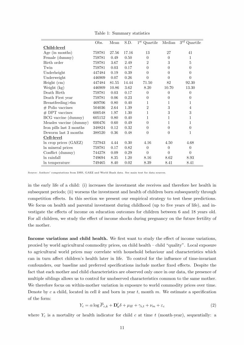
Table 1: Summary statistics

Obs. Mean S.D. 1st Quartile Median 3rd QuartileChild-levelAge (in months) 759781 27.56 17.16 13 27 41Female (dummy) 759781 0.49 0.50 0 0 1Birth order 759781 3.67 2.49 2 3 5Twin 759781 0.03 0.17 0 0 0Underheight 447484 0.19 0.39 0 0 0Underweight 446909 0.07 0.26 0 0 0Height (cm) 447484 81.55 14.44 71.50 82 92.30Weight (kg) 446909 10.86 3.62 8.20 10.70 13.30Death Birth 759781 0.03 0.17 0 0 0Death First year 759781 0.06 0.23 0 0 0Breastfeeding>6m 469706 0.80 0.40 1 1 1# Polio vaccines 504036 2.64 1.39 2 3 4# DPT vaccines 600548 1.97 1.30 1 3 3BCG vaccine (dummy) 605152 0.80 0.40 1 1 1Measles vaccine (dummy) 600476 0.60 0.49 0 1 1Iron pills last 3 months 348824 0.12 0.32 0 0 0Deworm last 3 months 388520 0.36 0.48 0 0 1Cell-levelln crop prices (GAEZ) 727943 4.44 0.30 4.16 4.50 4.68ln mineral prices 759781 0.17 0.82 0 0 0Conflict (dummy) 744278 0.09 0.29 0 0 0ln rainfall 749694 8.35 1.20 8.16 8.62 8.93ln temperature 749465 8.40 0.02 8.39 8.41 8.41

Source: Authors’ computations from DHS, GAEZ and World Bank data. See main text for data sources.

in the early life of a child: (i) increases the investment she receives and therefore her health in

subsequent periods; (ii) worsens the investment and health of children born subsequently through

competition effects. In this section we present our empirical strategy to test these predictions.

We focus on health and parental investment during childhood (up to five years of life), and in-

vestigate the effects of income on education outcomes for children between 6 and 18 years old.

For all children, we study the effect of income shocks during pregnancy on the future fertility of

the mother.

Income variations and child health. We first want to study the effect of income variations,

proxied by world agricultural commodity prices, on child health – child “quality”. Local exposure

to agricultural world prices may correlate with household behaviour and characteristics which

can in turn affect children’s health later in life. To control for the influence of time-invariant

confounders, our baseline and preferred specifications include mother fixed effects. Despite the

fact that each mother and child characteristics are observed only once in our data, the presence of

multiple siblings allows us to control for unobserved characteristics common to the same mother.

We therefore focus on within-mother variation in exposure to world commodity prices over time.

Denote by c a child, located in cell k and born in year t, month m. We estimate a specification

of the form:

Yc = α logP c,k + D′cδ + µH + γi,t + νm + εc (2)

where Yc is a mortality or health indicator for child c at time t (month-year), sequentially: a

11

dummy for under-height, which equals 1 if the height-for-age ratio is at least 3 standard deviations

below the corresponding z-score from WHO; a dummy for under-weight, which equals 1 if the

weight-for-age ratio is at least 3 standard deviations below the corresponding z-score from WHO;9

the continuous measures of height and weight relative to the WHO reference values (in logs); a

dummy for death at birth; a dummy for death in the first year; and a dummy for being alive at

the time of the survey.

Pk,t is the average of the monthly prices of crops produced in cell k during the in-utero period

and in the first year of life (or only during-in utero period when the dependent variable is death

at birth). We will also separate the in-utero and first year of life periods, as well as consider

subsequent years. Our results show that pregnancy and first-year prices generally have similar

effects, while prices in later years have a much lower impact. D′c is a vector of child characteristics

– age and age squared (in months), gender, twin, birth order. µH are mother fixed effects. In

our sample, using household fixed effects instead produces very similar results, as 89% of the

households in the sample contain only one mother (and 98% contain two mothers at most). γi,t

and νm are additional fixed effects accounting for country (i) ×year (t) of birth, and month-of-

birth unobserved factors affecting child health that might be correlated with crop prices. γi,t in

particular controls for all country-wide shocks in utero and in the first year of life that might

affect health, such as global economic conditions or civil wars. In our sensitivity analysis we will

additionally include controls for local weather shocks and other commodity prices shocks (oil and

mineral prices in oil or mineral producing regions) that might correlate with P c,k.

In eq. (2), α is our coefficient of interest. It can be interpreted as the effect of the local price of

produced crops on child mortality and health, relative to other children having the same mother.

Put differently, the coefficient tells us whether children born during periods of high crop prices

are in better health than their siblings. Identifying α requires observing at least two children per

mother, i.e. the sample is restricted to households with at least two siblings born over the 5 years

before the survey.

When Yc measures child health, α could either reflect a contemporaneous effect – a high

family income during pregnancy and the first year of life improves health at birth and in the

first year of life –, or a longer-term impact – beyond their contemporaneous effects, early life

income fluctuations affect child health after several years. To answer this question, we estimate

the following variant of eq. (2):

Yc =

4∑a=0

αaAgeac × log Pk,t + D′cδ + µH + γi,t + νm + εc (3)

where Ageac are dummies which equal 1 if the child is aged a = (0, 4) years at the time of the

survey. Since we have anthropometric data on children up to five years of age, we cannot test for

the significance of early-life income fluctuations to children’s health later in life. The profile of

the αa however informs us about the persistence of early life shocks on health. As an additional

test, we can also use the sample of children older than five and for whom we have information

on school attendance. In specifications similar to that of eq. (2) but with school attendance as

dependent variable, we can identify the effect of early exposure to income variations on education

9These definition correspond to “severe” underweight and stunting. Results available upon request are similarwhen “moderate” underweight and stunting are considered, i.e. two standard deviations below mean.

12

outcomes.

Parental investments in child health. Specifications (2) and (3) estimate the health ef-

fects of early life price shocks, and whether these are persistent. This persistence could come

from the direct effect of better nutrition on health and from other health investments. If, as in

the theoretical discussion, health investments complement initial conditions or investments, we

would expect parents to spend more on the health of their children born during good times –

compared to their siblings, potentially in a durable way.

We examine the parental investment responses by looking at whether exposure to the world

prices of commodities in utero and during the first year of life affects the parents’ investments in

the child’s health, and for how long. Specifically, we run a specification akin to (2), but replace

the dependent variable with a health investment measure:

Ic = β logP c,k + D′cδ + µH + γi,t + νm + εc (4)

where Ic is either a dummy for durable breastfeeding (longer than 6 months); the count of doses

of vaccines against polio, DPT, tuberculosis (BCG) and measles; or an indicator for provision

of iron pills or deworming in the last three months.10 A significant β coefficient would suggest

that at least part of the effects on children’s health that we estimate in eq. (2) is going through

parental investments – the Ic variables could be seen as ‘bad’ controls in specification (2) (Pei

et al., 2019).

We also estimate a variant of eq. (4) where the β are split by child age category, similar to

what we do for the health indicators in specification (3). This allows us to determine whether

the effect of early life shocks on health investment across children is persistent, which itself is an

indication of whether early and later life investments are complements. This specific exercise is

relevant to the administration of iron and deworm pills, which is observed at the current age of the

child. It makes little sense in the case of breastfeeding and vaccinations, which are investments

typically taking place upon birth or in the first year of life.

Sibling effects. Eqs. (2) to (4) feature mother fixed effects, i.e. they provide estimates that we

can only interpret in relative terms, across children born from the same mother. To investigate

further these intra-household adjustments, we modify the baseline specification and isolate sibling

effects (Adhvaryu and Nyshadham, 2016). This allows us to directly test Proposition 2 from the

theoretical framework: subsequent preferential investment in the ‘sweet child’ should decrease

resources available for the other children.

The within-mother estimates exploit variation in the producer price P received by child c

relative to the average producer price received by all the siblings. Therefore, any effect of exposure

to producer prices in early life compounds the effect of the ‘own’ price (received by child c) and that

of the siblings’ prices (received by all siblings in the households). To disentangle the contributions

10Adhvaryu and Nyshadham (2016) uses a similar set of variables to proxy for investment in child health. TheDHS also contains a variable coded one if the child received Vitamin A over the last three months: results obtainedusing this outcome variable are similar to the ones presented in the paper.

13

of these two components, we estimate specifications of this form (e.g., for health outcomes):

Yc = α logP c,k + αs logPsc,k + D′cβ + C′Hγ + µk + γi,t + νm + εc (5)

with the s superscript indicating the average of P across the older siblings of child c. Including

the price received by older siblings requires relaxing the within-mother specification. The mother

fixed effects (µH in eq. (2)) are replaced by cell fixed effects (µk) in eq. (5). The estimation

sample in eq. (5) therefore includes also children with no siblings.11 We collect controls for

the mother’s age (and its value squared), level of educational attainment (dummies for primary,

secondary and tertiary education), and for her household’s wealth index provided by the DHS

(dummies for the quintiles of the estimated wealth distribution) in the term CH . A similar spec-

ification is estimated also for health investment outcomes. The coefficient αs indicates whether

having siblings born in ‘good’ times (high Psk,t) affects the health of child c (conditional on her

own price, Pk,t). Both the evolutionary and economic logics predict α and αs to be of opposite

signs: α > 0 and αs < 0.

Econometric issues. We estimate all specifications using least squares; this is the preferred

estimator, despite the fact that the dependent variables are often binary or categorical, due to

the large dimensions of fixed effects we include. Standard errors are clustered at the cell-level

in the baseline. In our robustness we allow the error term to be spatially correlated (within a

500km radius), as well as serially correlated.

There are three main threats to identification in eqs. (2) to (5). The first is omitted variables,

which might correlate with world prices and affect child health through channels other than

income. In our robustness exercises, we will control for various potential time-varying confounders,

such as mineral and oil prices, conflicts and weather shocks. The second threat is selection. In

particular, our results suggest that early life income variations affect survival probabilities, which

can impact in turn our estimates on survivors’ health and parental investments. In our robustness

exercises, we will directly control for selection due to endogenous mortality. The third threat is

persistence in prices over time. If early life prices are strongly correlated with later life prices,

eqs. (2) to (5) might wrongly capture the effect of later prices. We will show that our results are

similar when controlling for the full sequence of prices, from the in utero period to the current

age of the child.

4.2 Results

Income and child health. Table 2 shows the estimates of the effect of exposure to world prices

of produced crops on child health and mortality – coefficient α in specification (2). All regressions

exploit within-mother variation, and control for the age (in months) and its value squared, gender

and birth order of the child, and whether the child is a twin – the coefficients on these controls are

not reported for brevity. Overall, children’s health is positively associated to increases in world

prices of locally produced commodities in early life. Children exposed to higher crop prices during

pregnancy and the first year of life have higher weight and height relative to standard reference

values, and are less likely to be stunted or underweight. In our baseline specification, exposed

11Restricting the sample to children with at least one sibling, as we do in the within-mother estimations, givesequivalent results (available upon request).

14

children seem also significantly less likely to die at birth or during the first year of life during

high income periods. They are more likely to survive later on as well, at the time of the survey.

These results on mortality and survival are however not robust to alternative specifications and

data sources, as discussed in section 4.3.

Table 2: Exposure to world crop prices and child health

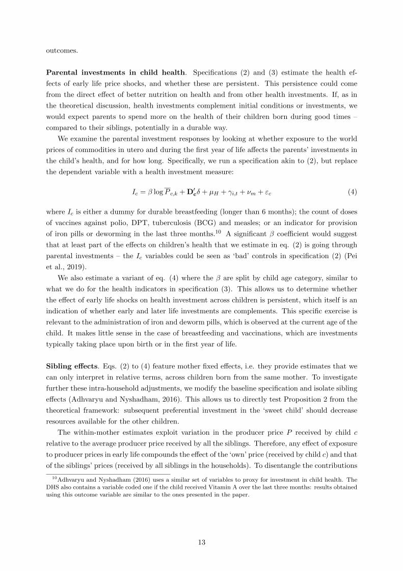
(1) (2) (3) (4) (5) (6) (7)Dep. var. Underheight Underweight ln height ln weight —— Death —— Alive at t

1st year At birth

ln crop price -0.226a -0.180a 0.068a 0.135a -0.008b -0.019a 0.026a

(0.042) (0.028) (0.010) (0.021) (0.003) (0.006) (0.007)

Obs. 191823 191513 191795 191487 2256856 2256856 2256856R2 0.627 0.586 0.756 0.749 0.281 0.282 0.306Child controls Yes Yes Yes Yes Yes Yes YesMother FE Yes Yes Yes Yes Yes Yes Yes

c significant at 10%; b significant at 5%; a significant at 1%. OLS estimations. The unit of observation is a child. Standard errors clustered atthe cell level in parentheses. All estimations include child controls, mother fixed-effects, country × year-of-birth and month-of-birth dummies.Child controls include: gender, birth order, twin dummy, age in month, and its value squared. ln crop price index is the log of the world priceof the crops produced in the cell, weighted by the share of each crop in the area, averaged over in utero period and first year of life. In column(5), it is average over the in utero period only. Underheight (respectively underweight) is a dummy which equals 1 if the height-for-age (resp.weight-for-age) ratio is at least 3 standard deviations below the z-score from WHO. ln height (resp. ln weight) are the logs of height (resp.weight) divided by the gender-specific average height (resp. weight) for that particular age in month from WHO. Death is a dummy whichequals 1 if the child dies at birth (col. 5) or in her/his first year (col. 6), 0 otherwise. Alive at t is a dummy that equals 1 if the child is aliveat the time of the survey (t).

The estimated coefficients imply sizeable effects of differences in the local level of world prices

at birth. Consider the effects on children’s height (column (3)). In the estimation sample, the

healthiest child in the family is 7% taller than the ‘shortest’ one (height is standardised by age and

sex). The estimated elasticity in column (3) thus suggests that the least healthy sibling could have

erased completely the height gap if she would have received a 100% higher crop price than the one

received by the healthiest sibling in early life (conditional on the crop prices received by the other

siblings). The average within-mother spread in the crop price variable being 20%, our estimates

predict that price-related income fluctuations could explain up to 20% of the average differences

in height across siblings. Using the estimates from the linear probability model from column (1),

we obtain that the 20% higher crop price in early life can lead to 4 percentage-point lower risk of

severe stunting. The same calculations lead to somewhat smaller yet important magnitudes for

the impact on weight – e.g., differences in early exposure to world prices of produced commodities

can explain 10% of the differences in weight across siblings.

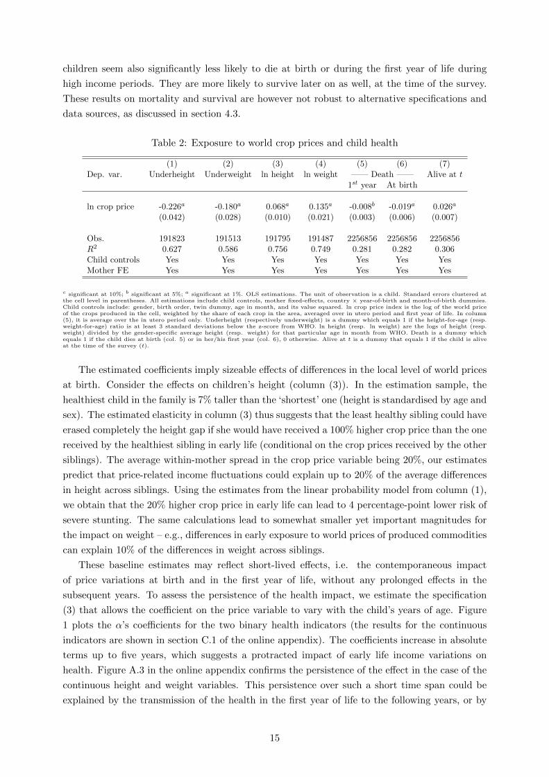
These baseline estimates may reflect short-lived effects, i.e. the contemporaneous impact

of price variations at birth and in the first year of life, without any prolonged effects in the

subsequent years. To assess the persistence of the health impact, we estimate the specification

(3) that allows the coefficient on the price variable to vary with the child’s years of age. Figure

1 plots the α’s coefficients for the two binary health indicators (the results for the continuous

indicators are shown in section C.1 of the online appendix). The coefficients increase in absolute

terms up to five years, which suggests a protracted impact of early life income variations on

health. Figure A.3 in the online appendix confirms the persistence of the effect in the case of the

continuous height and weight variables. This persistence over such a short time span could be

explained by the transmission of the health in the first year of life to the following years, or by

15

the response of parental health investment. We now explore this latter possibility.

Figure 1: Exposure to world crop prices and child health over time

(a) Underheight (b) Underweight

−.4

−.3

−.2

−.1

0

[0,1] [1,2] [2,3] [3,4] [4,5]Age category

Effect of early life income shocks on health

−.2

5−

.2−

.15

−.1

−.0

50

[0,1] [1,2] [2,3] [3,4] [4,5]Age category

Effect of early life income shocks on health

Source: These figures report the coefficient on the ln crop price variables price, split by child age in years, based on the estimation of eq. (3).Shaded areas are 90% confidence bands.

Income and health investment. Table 3 shows the estimates of specification (4), which

assesses the impact of income-related price fluctuations on different forms of health investments

in children. This exercise speaks directly to the main prediction of our theoretical framework

(Proposition in 1 in section 2): parental investments should increase with the child’s initial

income conditions. By adopting the same specification of the health regression (see eqs. (2) and

(4)), we can determine whether the estimates found in Table 2 solely reflect better nutrition and

persistence in health conditions, or also a behavioral response of parents through investments in

health.

Overall, the results point to a positive effect of exposure to world prices at birth on vaccinations

and other investments in the health of children (controlling for their age, gender, birth order and

for twin status). The evidence is consistent with parents responding to crop price variations in

the early life of the child by investing more in her health. The size of the implied effects is non-

negligible. The largest gap in the number of Polio vaccination doses across siblings (dependent

variable in column (2)) is on average 0.91. The estimated crop price coefficient in column (2)

suggests that this gap would be 5% lower (0.86) if the crop price index at birth for the low-polio

child were 20% higher – the sample average largest gap in the price index across siblings. The

same within-household changes in prices is associated with a small 1 percentage-point higher

likelihood of receiving vaccination against tuberculosis (BCG), and a 4 percentage-point higher

chances of being immunized against measles (7% of the sample average). A 20% higher crop

price early in life is also associated with a 4 percentage-point higher likelihood of being breastfed

for at least six months (8.5% of the sample probability). The null effect on the probability of

giving iron pills is not surprising, given that this treatment is recommended to children in school

age (older than five), who are not included in the sample. Importantly, children who were born

during periods of high crop prices relative to their siblings are significantly more likely to receive

16

deworming treatments – an effect equivalent to 6% of the sample probability.

Table 3: Exposure to world crop prices and health investments

(1) (2) (3) (4) (5) (6) (7)Dep. var. Breast. – Vaccines (# doses) – – Vaccines – Other investments

Polio DPT BCG Measles Iron Deworm

ln crop price 0.178a 0.211c 0.331a 0.065b 0.201a 0.015 0.108a

(0.058) (0.110) (0.096) (0.027) (0.038) (0.022) (0.037)

Obs. 152427 247317 276227 278902 275395 185373 203771R2 0.796 0.813 0.821 0.804 0.797 0.817 0.822Child controls Yes Yes Yes Yes Yes Yes YesMother FE Yes Yes Yes Yes Yes Yes Yes

c significant at 10%; b significant at 5%; a significant at 1%. OLS estimations. In the first column the dependent variable takes the value 1 isthe child has been breastfed for at least 6 months, 0 otherwise. In the next two columns the dependent variables are the number of doses takenby the child of Polio (max. 4 doses), and DPT (max. 3 doses). In columns (4) to (7) the dependent variables are dummies taking the value 1if the child has taken all required doses of particular vaccines (Measles and DPT), iron pills, and deworming drugs (these last two during thethree months preceding the survey).

The positive association between health investments in children and exposure to income vari-

ation in utero and at birth can be explained by a path-dependency in parents’ behaviour – they

had invested more into the child who received a good price in utero and at birth, and they kept

this behaviour over time. Economics and evolutionary theories are consistent with this path-

dependency. To shed light on this interpretation, in Figure A.4 of online appendix C.1 we split

again the effect of crop prices according to the age of the child at the time of the survey, similarly

to what we did for the health outcome specifications (see eq. (3) and the results in figure 1). We

do this for the last two indicators, iron pills and deworming, the other investments being typically

done in the first year of life. Overall, results suggest that the positive coefficient on crop prices is

stable or slightly increasing with age, though it is imprecisely estimated in the case of iron pills.

These results suggest that the differential health outcomes of siblings to income variations in

utero and at birth is partly driven by parental investment responses. At this stage, none of the

results however shows that investments in a child’s health and her health outcomes are directly

affected by the investments on her siblings, as predicted by the theoretical framework in section

2. We now test this prediction.

Sibling effects. Health outcomes and parental investment may react to the crop price received

by the child and to the crop prices received by the other siblings in early life. The within-mother

coefficients that are estimated in Tables 2 and 3 compound these two types of effect because

they rely on deviations in crop prices with respect to the average crop prices across siblings.

In Tables 4, we separate the income-related price of the child from the average income-related

price received by her older siblings (specification (5)). As in Adhvaryu and Nyshadham (2016),

the objective is to identify the contribution of the shock received by the siblings. The sibling

regression for parental investments (Panel B of Table 4) speaks directly to a prediction of the

economic framework and of the evolutionary theories summarized in Proposition 2, section 2.

The results, based on within-cell variation, reveal that sibling effects are significant and tend

to lower child health and parental investments.12 Child health decreases significantly with the

12The baseline results on children’s health and parental investments based on within-mother variation are con-

17

Table 4: Own and siblings’ exposure to world crop prices, child health, and parental investments

(1) (2) (3) (4) (5) (6) (7)Panel A: Child healthDep. var. Underheight Underweight ln height ln weight —— Death —— Alive at t

1st year At birth

ln crop price (own) -0.295a -0.198a 0.089a 0.195a -0.010a -0.016a 0.026a

(0.025) (0.016) (0.007) (0.015) (0.003) (0.005) (0.007)

ln crop price (older siblings) 0.032a 0.013a -0.004b -0.010a 0.000 0.002 -0.009a

(0.006) (0.004) (0.001) (0.003) (0.002) (0.002) (0.003)

Obs 263635 261917 263612 261894 1611117 1611117 1611117R2 0.135 0.098 0.301 0.311 0.035 0.046 0.080

Panel B: InvestmentsDep. var. Breast. – Vaccines (# doses) – – Vaccines – Other investments

Polio DPT BCG Measles Iron Deworm

ln crop price (own) 0.470a 0.428a 0.538a 0.090a 0.168a 0.075a 0.184a

(0.041) (0.077) (0.064) (0.017) (0.025) (0.017) (0.025)

ln crop price (older siblings) -0.005 -0.062a -0.092a -0.011b -0.020a -0.010b -0.003(0.005) (0.018) (0.015) (0.005) (0.005) (0.005) (0.006)

Obs 271036 329136 370119 372696 370036 261528 291275R2 0.565 0.361 0.432 0.358 0.435 0.152 0.311Child controls Yes Yes Yes Yes Yes Yes YesMother controls Yes Yes Yes Yes Yes Yes YesCell FE Yes Yes Yes Yes Yes Yes Yes

c significant at 10%; b significant at 5%; a significant at 1%. The unit of observation is a child. Standard errors clustered at the cell level inparentheses. All estimations include country × year-of-birth and month-of-birth dummies. Child controls include: gender, birth order, twindummy, and age in month. Mother controls include: mother’s age and age square, education dummies, and dummies for quintiles of the wealthdistribution. ln crop price index is the log of the world price of the crops produced in the cell, weighted by the share of each crop in the area.ln crop price (older siblings) is the price faced on average by all elder siblings during in utero and during their first year of life. In PanelA: underheight (respectively underweight) is a dummy which equals 1 if the height-for-age (resp. weight-for-age) ratio is at least 2 standarddeviations below the z-score from WHO. Ln height (resp. ln weight) is the logs of height (resp. weight) divided by the gender-specific averageheight (resp. weight) for that particular age in month from WHO. Death is a dummy which equals 1 if the child dies at birth (col. 5) or inher/his first year (col. 6), 0 otherwise. Alive at t is a dummy that equals 1 if the child is alive at the time of the survey (t). In Panel B: In thefirst column the dependent variable takes the value 1 is the child has been breastfed for at least 6 months, 0 otherwise. In the next two columnsthe dependent variables are the number of doses taken by the child of Polio (max. 4 doses), and DPT (max. 3 doses). In columns (4) to (7)the dependent variables are dummies taking the value 1 if the child has taken all required doses of particular vaccines (Measles and DPT), ironpills, and deworming drugs (these last two during the three months preceding the survey.

price in utero and at birth received by the older siblings, whereas there is no sibling effect on

mortality (Panel A). Parents invest less in the health of a child if her older siblings were exposed

to a higher prices in utero and at birth (Panel B). These results are consistent with theoretical

expectations: parental investments in the health of a child decrease with the income received at

birth by her older siblings (and hence with their quality). Parents invest less on a child if the

other siblings are ‘fitter’ (as evolutionary theories would suggest), and if these ‘fitter’ siblings

attract relatively more resources (as economic logic would also suggest).

4.3 Sensitivity analysis

In this section, we show that our main findings – Tables 2, 3, and 4 – are confirmed in a large

firmed in less stringent specifications where we exploit variation within the cell (as in the siblings regressions). Theresults, reported in Table A.3 of the Online Appendix, thus suggest that the effects of early exposure to higherincome are valid across children of different mothers and households.

18

battery of sensitivity checks. Most of the tables are relegated to the online appendix (section C),

where we discuss these results extensively.

Selection through mortality. The samples that we use to estimate the health effects of

income-related variations are composed only of children who are observed at the time of the

surveys. This selection might influence the interpretation of our findings as the observed children

might be stronger and more responsive to health investments than the others who died prema-

turely. The mortality results in columns (5) to (7) of Table 2 show that indeed a higher income

in early life enhances survival prospects. In section C.4 of the online appendix, we investigate

directly the influence of selection through survival on the baseline health and parental invest-

ments results documented in Tables 2 and 3. The results show that our baseline findings remain

unaltered when we control for selection. Together with the estimated effects on mortality, these

findings tell us that the higher survival probability enjoyed by children born in periods of higher

income cannot explain the reinforcing health investment strategies of the parents (and the related

differential health outcomes of their children).

Full sequence of prices. Price are persistent over time. This persistence is an issue in our case,

as it implies that we might be capturing the effect of prices in subsequent years on subsequent

health and not the effect of early life prices on subsequent health. To solve this problem, we can

include the full sequence of prices in our estimations. The results are shown and discussed in

section C.5 of the online appendix. We find that (i) our results are statistically robust; (ii) preg-

nancy and first year prices have quantitatively similar effects; (iii) later-life prices, while being

generally significant, have a much more limited impact on health indicators.

Additional controls. Crop prices could correlate with other time-varying, cell-level variables.

For instance, Berman and Couttenier (2015) and McGuirk and Burke (2017) show that they

impact local conflict. In section C.6 we show that our estimates are virtually unchanged when we

control for other time-varying local variables such as exposure to world prices of locally produced

minerals, weather conditions (which have been used as income shifters, but are unlikely to co-vary

with our constructed price index of produced crops), and incidence of conflicts.

Cash/staple crops. Our empirical strategy and results are consistent with the interpretation

of variation in the crop price index as a shifter of local income. The alternative approach would

be to think of our price variable as affecting households as consumers. This would however imply

that child health deteriorates with exposure to higher prices of the supposedly ‘consumed’ crops,

which counters our baseline findings. Our estimates could still provide a ‘net’ effect that masks

the counteracting influence of the price of some consumed crops. To check for this possibility, we

split our price index (see eq. (1)) into the constructed local price of “cash” crops as defined by

McGuirk and Burke (2017) (in our sample, cocoa, coffee, cotton, tea and tobacco) – which should

be mainly for production –, and the other crops – which could be also consumed. In the online

appendix section C.7 we report the results from a specification where the two price variables

are included simultaneously as determinants of child health. The coefficients on the ‘food’ crop

price variable has the same sign of and is of similar size to the coefficient on the cash crop price

19

variable, although the cash crop variables’ coefficients are less precisely estimated in the case of

health investments. This reflects the fact that cash crops account for a small part of our sample.

Overall, these results corroborate our empirical assumption that the set of crops in our sample

are mainly produced and hence variation in their prices should reflect producers’ income (through

land suitability).

Long-term persistence. Our baseline results are restricted to children, and in that sense

do not speak about the long-term health effect of early life income variations. In section C.8

of the online appendix we estimate the effect of these income variations on adult health. We

consider anthropometric information on adults contained in the DHS. We cannot control for

household fixed effects in these estimations, as adult members are likely to have left their initial

household and to live away from their siblings. We thus rely on within-cell variation in this exer-

cise, and confirm that the effect of early life shocks persists in the long-run consistent with a vast

literature (summarised in Almond et al., 2018), which has mostly relied on single-country studies.

Other robustness. In sectionC.9 of the online appendix we use an alternative measure of

agricultural specialization from the M3-CROP database (Monfreda et al., 2008). Prices are in

this case weighted by the share of harvested area in the cell around 2000. In section C.10 we

deal with potential migration by restricting our sample to a subset of the households that did

not migrate since the birth of the child. Finally, in section C.11 we allow the errors term to be

spatially correlated within a 500km radius (Conley, 1999).13 Our main findings go through these

additional robustness checks.

4.4 Other parental investments

Our conceptual framework discusses the drivers of parents’ investment decisions in children’s

health within the family. Similar mechanisms should nonetheless apply to other types of parental

investments affecting the parents’ objective function (genetic transmission in evolutionary theo-

ries, or future income in the economics literature).

First, while good health is a necessary condition for genetic transmission, most of the research

in economics on parental investments has focused on education (e.g., see the review by Almond

et al., 2018). In columns (1)-(3) of Table 5, we thus test whether our baseline results on health

hold also for children’s education. In particular, we regress an indicator for school attendance for

children in school age on the crop price variable measured during the in-utero period and the first

year of life. As for our baseline specifications (e.g., eq. (2)), we exploit within-mother variation

and control for children’s characteristics such as gender, age, birth order and twin status. The

results show that children who received a higher income-related price at birth are significantly

more likely to attend school. The reinforcing investment strategies found for health are thus

confirmed for children’s education, bolstering the validity of our baseline results.14 In this case,

however, parents’ investments in the ‘strong’ older siblings do not affect directly school attendance

13The estimations in this section are based on the STATA package acreg developed by Colella et al. (2019).14Yi et al. (2015) find evidence for compensating health investments, and for reinforcing education investments,

in their Chinese sample of twins.

20

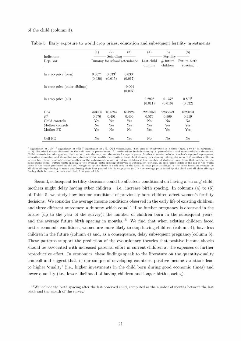
of the child (column 3).

Table 5: Early exposure to world crop prices, education and subsequent fertility investments

(1) (2) (3) (4) (5) (6)Indicators ———– Schooling ———– ———– Fertility ———–Dep. var. Dummy for school attendance Last child # future Future birth

dummy children spacing

ln crop price (own) 0.067a 0.033b 0.030c

(0.020) (0.015) (0.017)

ln crop price (older siblings) -0.004(0.007)

ln crop price (all) 0.292a -0.137a 0.807b

(0.011) (0.016) (0.322)

Obs. 763006 814394 634924 2236859 2236859 1620493R2 0.676 0.401 0.400 0.576 0.969 0.919Child controls Yes Yes Yes No No NoMother controls No Yes Yes Yes Yes YesMother FE Yes No No Yes Yes Yes

Cell FE No Yes Yes No No No

c significant at 10%; b significant at 5%; a significant at 1%. OLS estimations. The unit of observation is a child (aged 6 to 17 in columns 1to 3). Standard errors clustered at the cell level in parentheses. All estimations include country × year-of-birth and month-of-birth dummies.Child controls include: gender, birth order, twin dummy, and dummies for age in years. Mother controls include: mother’s age and age square,education dummies, and dummies for quintiles of the wealth distribution. Last child dummy is a dummy taking the value 1 if no other childrenis ever born from that particular mother in the subsequent years. # future children is the number of children born from that mother in thesubsequent years. Future birth spacing is the average birth spacing observed in subsequent periods. ln crop price index is the log of the worldprice of the crops produced in the cell, weighted by the share of each crop in the area. ln crop price (siblings) is the price faced on average byall elder siblings during in utero and during their first year of life. ln crop price (all) is the average price faced by the child and all elder siblingsduring their in utero periods and their first year of life.

Second, subsequent fertility decisions could be affected: conditional on having a ‘strong’ child,

mothers might delay having other children – i.e., increase birth spacing. In columns (4) to (6)

of Table 5, we study how income conditions of previously born children affect women’s fertility

decisions. We consider the average income conditions observed in the early life of existing children,

and three different outcomes: a dummy which equal 1 if no further pregnancy is observed in the

future (up to the year of the survey); the number of children born in the subsequent years;

and the average future birth spacing in months.15 We find that when existing children faced

better economic conditions, women are more likely to stop having children (column 4), have less

children in the future (column 4) and, as a consequence, delay subsequent pregnancy(column 6).

These patterns support the prediction of the evolutionary theories that positive income shocks

should be associated with increased parental effort in current children at the expenses of further

reproductive effort. In economics, these findings speak to the literature on the quantity-quality

tradeoff and suggest that, in our sample of developing countries, positive income variations lead

to higher ‘quality’ (i.e., higher investments in the child born during good economic times) and

lower quantity (i.e., lower likelihood of having children and longer birth spacing).

15We include the birth spacing after the last observed child, computed as the number of months between the lastbirth and the month of the survey.

21

5 Heterogeneity

An advantage of our empirical setting is the availability of comparable data on children’s

health and parental investments across 54 developing countries. We exploit this feature of the

data and allow the coefficient on the price variable to vary across countries. This exercise serves

also as a further check on the stability of our findings across regions. The results for our main

measures of child health, underweight and underheight, are reported in Figure A.6 of the online

appendix (section C.12). Two conclusions arise. First, in most countries the estimates are of the

same sign as in our baseline results of Table 2; more precisely, they are of the same sign (negative

for the underweight and underheight variables, positive for the log weight and height) in 62-73%

of the cases depending on the specification. This suggests that our results are not driven by a few

specific countries. Second, important heterogeneity exists across countries: in some countries,

the effect is reversed; in many others, it is not statistically significant.

What drives this heterogeneity? As discussed in section 2, two types of country characteristics

may matter. First, the level of development of financial markets, which affects households’ ability

to borrow. The economic framework outlined in section 2 and detailed in the online appendix

rests on the assumption of imperfect capital markets. Households are not allowed to borrow or

lend. If they could, parents would be able to smooth income changes and neutralise any long-term

impact of income variations during the early life of their children. We use World Bank data on

private credit over GDP as a proxy for financial development.16

Second, in evolutionary theories, the level of social competition for resources is a key factor.

Under competitive environments, parents tend to invest more in offsprings with the best genetic

fitness – in our case, those who experienced good in utero and early life income conditions. This

is because such individuals are more likely to succeed in future competitions. As a proxy for the

competitiveness of the environment, we use mortality rates for children with at most 5 years of

age, from the World Bank Development Indicators. The idea is that high mortality rates signal

high competition for survival, and thus make early parental investments important for future

success.

For each indicator we divide countries into quintiles and interact our early life income shock

with each of the quintile dummies. The results are reported in Figure 2 below, and in Figures

A.7 and A.8 in the online appendix C.12. Figure 2 represent, for each country-specific proxy, the

effect of income variations split by quintile, on each of the binary health and health investment

measures.17

16All our country-specific proxies are time-invariant, and computed as the averages of the variable since 1990.17We restrict our analysis to binary measure to permit comparability of the estimates across measures

22

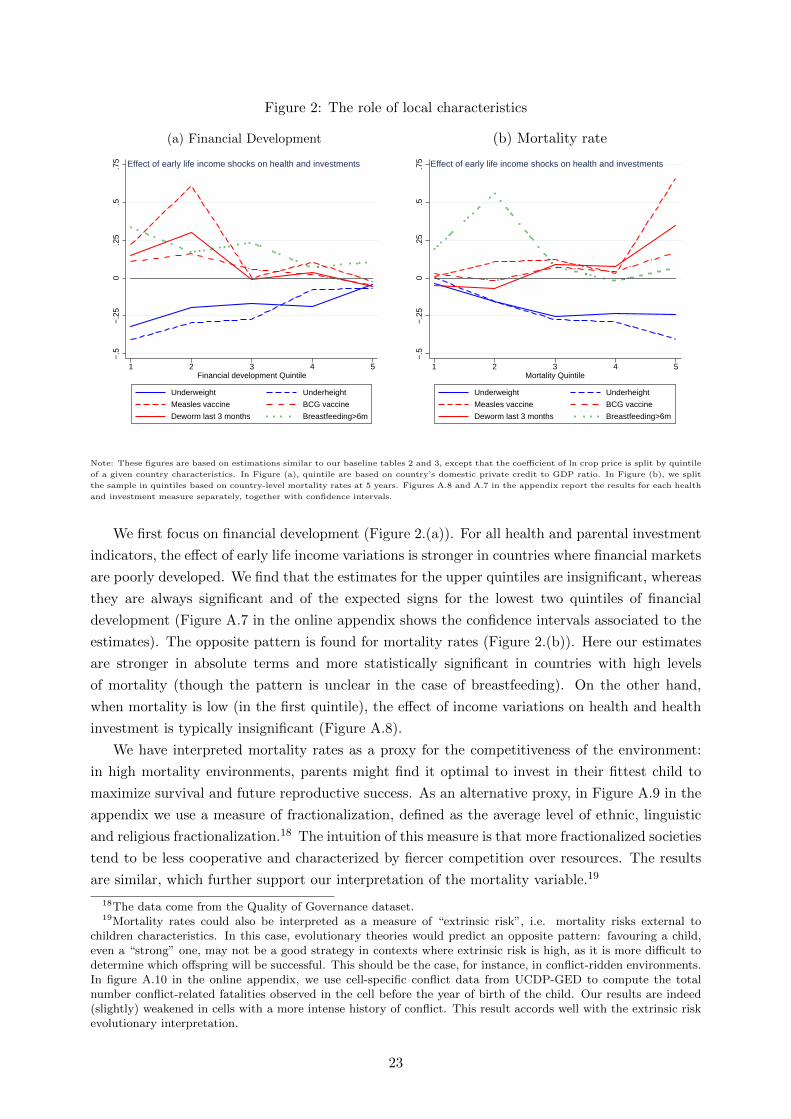
Figure 2: The role of local characteristics

(a) Financial Development (b) Mortality rate

−.5

−.2

50

.25

.5.7

5

1 2 3 4 5Financial development Quintile

Underweight Underheight

Measles vaccine BCG vaccine

Deworm last 3 months Breastfeeding>6m

Effect of early life income shocks on health and investments

−.5

−.2

50

.25

.5.7

5

1 2 3 4 5Mortality Quintile

Underweight Underheight

Measles vaccine BCG vaccine

Deworm last 3 months Breastfeeding>6m

Effect of early life income shocks on health and investments

Note: These figures are based on estimations similar to our baseline tables 2 and 3, except that the coefficient of ln crop price is split by quintile

of a given country characteristics. In Figure (a), quintile are based on country’s domestic private credit to GDP ratio. In Figure (b), we split

the sample in quintiles based on country-level mortality rates at 5 years. Figures A.8 and A.7 in the appendix report the results for each health

and investment measure separately, together with confidence intervals.

We first focus on financial development (Figure 2.(a)). For all health and parental investment

indicators, the effect of early life income variations is stronger in countries where financial markets

are poorly developed. We find that the estimates for the upper quintiles are insignificant, whereas

they are always significant and of the expected signs for the lowest two quintiles of financial

development (Figure A.7 in the online appendix shows the confidence intervals associated to the

estimates). The opposite pattern is found for mortality rates (Figure 2.(b)). Here our estimates

are stronger in absolute terms and more statistically significant in countries with high levels

of mortality (though the pattern is unclear in the case of breastfeeding). On the other hand,

when mortality is low (in the first quintile), the effect of income variations on health and health

investment is typically insignificant (Figure A.8).

We have interpreted mortality rates as a proxy for the competitiveness of the environment:

in high mortality environments, parents might find it optimal to invest in their fittest child to

maximize survival and future reproductive success. As an alternative proxy, in Figure A.9 in the

appendix we use a measure of fractionalization, defined as the average level of ethnic, linguistic

and religious fractionalization.18 The intuition of this measure is that more fractionalized societies

tend to be less cooperative and characterized by fiercer competition over resources. The results

are similar, which further support our interpretation of the mortality variable.19

18The data come from the Quality of Governance dataset.19Mortality rates could also be interpreted as a measure of “extrinsic risk”, i.e. mortality risks external to

children characteristics. In this case, evolutionary theories would predict an opposite pattern: favouring a child,even a “strong” one, may not be a good strategy in contexts where extrinsic risk is high, as it is more difficult todetermine which offspring will be successful. This should be the case, for instance, in conflict-ridden environments.In figure A.10 in the online appendix, we use cell-specific conflict data from UCDP-GED to compute the totalnumber conflict-related fatalities observed in the cell before the year of birth of the child. Our results are indeed(slightly) weakened in cells with a more intense history of conflict. This result accords well with the extrinsic riskevolutionary interpretation.

23

Overall, these results lend additional support to the economic and evolutionary theories dis-

cussed earlier. They show that the effect of early life income variations on parental investments

and children’s health within households depends on country characteristics, in particular on the

development of financial markets and on the level of socio-economic competition. This evidence

is suggestive and has to be taken with caution, as our sample of countries is relatively small and

our proxies are indirect and likely to be correlated with other country characteristics.

6 Child health inequality and policy targeting

The results of the child-level regressions have important implications for aggregate inequalities

in child health. A direct implication is that health disparities within households increase with

disparities in prices in utero and at birth across. In this section, we assess the importance of

local variations in the prices of produced crops for aggregate disparities in child health outcomes

that come from within the household. The within-household dimension is all the more important

when it comes to the targeting of poverty reduction policies, which often take (under)nutrition

as a key poverty indicator. These policies usually target poor households, under the implicit

assumption that economic and nutritional outcomes are the same within the household. This

strategy and hence the effectiveness of the interventions can thus be jeopardized by changes in

the socioeconomic environment (such as income fluctuations) that have asymmetric nutritional

and health effects across household members (in our setting, across siblings).

To measure disparities in child health, we use the underweight and underheight indicators,

which are employed to evaluate the nutritional status of children. For each indicator, we iden-

tify three types of households at the time of the DHS surveys: (i) those where all children

are underweight(height) (‘all-underweight(height)’); (ii) those where not all children are under-

weight(height) (‘mix-underweight(height)’); and (iii) those where none of the children is under-

weight(height) (‘none-underweight(height)’). Within countries, our measure of local disparities

in children’s nutritional status is the share of households in an administrative region (Admin2 )

that is classified under each of the three categories. Intuitively, an increase in within-household

inequality in child health should lead to a higher share of households where children have dif-

ferent nutritional status. While this regional variable might not identify the influence of small

differential changes in nutritional outcomes across children, it reflects the regional consequences

of within-households disparities and speaks directly to the policy issue of targeting. Changes in

these shares over time are the outcome variable in the following region-level regression:

∆ShareDrt = αD|∆ log Pr,t|+4∑

a=2

αDa |∆ log Pa,r,t|+ βD∆D′rt + µt + γn + εDrt (6)

where the unit of observation is now an administrative region r at time t. ∆ denotes the first-

difference operator, and D indicates one of the three possible shares. To observe changes at the

regional level, the estimation sample includes countries with at least two DHS surveys. Since we

have data on children up to five years of age, we take a five-year cohort as the time unit. The

variable ∆Share thus equals the change in, say, the ‘mix-underweight(height)’ share of households

in region r between two five-year cohorts of children.

The main variable of interest, |∆ logP r,t| is the absolute value of the (changes in) average

24

prices faced by the cohort of children born in region r in the five years preceding the survey date,

during the in utero period and their first year of life. The coefficient αD captures the association

between changes in child health inequality and changes in the average price in early life across

cohorts. The first-difference specification wipes out time-invariant factors that are specific to

region r. Within a five-year cohort, the prices faced in utero and in the first year of life by

a child who is, say, two, are the second-year prices of a child who is four. The αD coefficient

might thus pick up the effects of prices at different stages of children’s early life. To correct for

this, we control for the changes (in absolute value) in average prices faced by children in their

second, third, and fourth year of life (the ∆ log Pa,r,t term in eq. (6)). The term Drt collects

first-differences of cohort-averaged characteristics (age in months, proportion of female children,

of twins, and average number of children per household), and µt and γn are year of birth and

country dummies controlling for aggregate trends.

Figure 3 depicts the estimated coefficient on the price volatility variable in our baseline spec-

ification (αD), and in a robustness check where we replace the country dummies with country-

year-of-survey ones. Because the household categories are mutually exclusive, the sum of the

coefficients across category shares must equal zero. The results underscore a pro-inequality effect

of early exposure to price variations within the household. The share of households where only

some children suffer from malnutrition increases with variations in average prices that children

faced in utero and during the first year of life within a region.

Figure 3: Exposure to world crop prices and child health inequality at the regional level

(a) Underweight (b) Underheight

.013

-.0067

-.2

-.19

.19

.19

Share w/all children below / Baseline

Rob.

Share w/no children below / Baseline

Rob.

Share w/some children below / Baseline

Rob.

-.4 -.2 0 .2 .4

.13

.14

-.42

-.32

.29

.18

Share w/all children below / Baseline

Rob.

Share w/no children below / Baseline

Rob.

Share w/some children below / Baseline

Rob.

-.6 -.4 -.2 0 .2 .4

These figures report the coefficient on the ln crop price variable – the absolute value of the (changes in) average prices faced by the cohort of

children born in region r in the five years preceding the survey date, during the in utero period and their first year of life –, i.e. αD in thebaseline regression (6). The “Rob.” specifications replace country dummies with country-year-of-survey fixed effects. All regressions include:changes (in absolute value) in average prices faced by children in their second, third, and fourth year of life; changes in average age in months,proportion of female children, of twins, and average number of children per household; and year-of-birth dummies. Bars represent 90% confidenceintervals.

To assess the quantitative relevance of these results, we use our regression model in (6) to

compute the changes in the predicted average shares for each household category and country in

our sample under two scenarios. First, we predict shares assuming that there was no change in

average crop prices at birth and in utero – i.e., we set |∆ log Pr,t| = 0 in equation (6). This is

equivalent to an hypothetical situation where two consecutive cohorts of children faced the same

early-life prices within a region. In the second scenario, we simply use the predictions of the

regression model using observed price variations. The region-level predictions are then averaged

25

across regions within countries to convey country-level predicted household category shares.20

Figure 4 shows the predicted change in each of the three categories of households: ‘no-

underweight (height)’, ‘mix-underweight (height)’, and ‘all-underweight (height)’. Price varia-

tions increase the share of ‘mixed’ households, where healthy and malnourished siblings co-exist.

The increase in the incidence of mixed households is quantitatively larger for underheight, or

stunting. The average region in our sample has 17 percentage-point higher ‘mix-underheight’

share of households when we include the effect of price volatility, relative to a situation without

any changes in crop prices in early life.21

Figure 4: Counterfactual: price variations and child health inequality at the country-level

(a) Underweight (b) Underheight

-.2 -.1 0 .1 .2

GuineaHaiti

BangladeshBurkina Faso

EgyptZimbabwe

SenegalCameroon

GhanaBenin

MaliJordanKenya

Cote d'IvoireDominican Rep.

LiberiaCongo, Dem. Rep.

ZambiaMalawiNigeria

RwandaEthiopiaUganda

NamibiaSierra Leone

TanzaniaPeru

Cambodia

Allchildren underweight

Nochild underweight

Somechildren underweight

Change in the share of HH with

-.4 -.2 0 .2 .4

GuineaHaiti

BangladeshBurkina Faso

EgyptZimbabwe

SenegalCameroon

GhanaBenin

MaliJordanKenya

Cote d'IvoireDominican Rep.

LiberiaCongo, Dem. Rep.

ZambiaMalawiNigeria

RwandaEthiopiaUganda

NamibiaSierra Leone

TanzaniaPeru

Cambodia

Allchildren underheight

Nochild underheight

Somechildren underheight

Change in the share of HH with

These figures report the within-country averages of predicted changes in each share of household, computed by comparing the case where|∆ log Pr,t| = 0 with the predictions using the actual price variations. Predicted shares at the region-time level are averaged within countries.

The higher relevance of households with children both below and above the malnutrition

thresholds owing to differing income situations at birth can have important policy implications.

In particular, targeting of poverty reduction interventions (e.g., to tackle children’s malnutrition

and stunting in rural areas) is problematic when economic and health conditions vary substan-

tially within the households – the primary unit of targeting. For example, consider an anti-poverty

programme tailored to eradicate children’s malnutrition that can only target households with at

least one undernourished child. Some of the beneficiary households would include children who

are not undernourished. The evidence from the child-level regressions tells us that in these house-

holds parents will tend to reinforce the existing health disparities among siblings, by investing

the additional resources (e.g., cash transfers) relatively more on the healthy ones. The evidence

from the region-level regressions suggests that the divergent health trajectories within the house-

hold will make targeting even more difficult, thereby fuelling further the ineffective allocation of

resources to tackle poverty and malnutrition. This case scenario shows how differential parental

20While indicative of the size of the effects, this exercise rests on some approximations. In particular, we are usingestimates that exploit within-country variation to obtain predictions at the country level. This would create bias inour predictions if crop suitability in one region affects exposure in neighbouring regions – e.g., if higher suitabilityof one region to produce high-price crops makes also producers in neighbouring regions with lower suitability moreexposed to world prices. For this reason, we treat the results of the exercise as suggestive of the magnitudesinvolved.

21In section A.11 we report the results in absolute terms, i.e. the predicted shares under each scenarios. Thisallows to see the actual levels of the shares in the two cases.

26

investments across siblings and their corresponding divergence in health outcomes can exacerbate

the targeting issue of anti-poverty interventions.

7 Concluding remarks

In this paper, we provide novel evidence on how fluctuations in local economic conditions can

shape the way parents allocate resources across siblings. Geo-localised survey health data for 54

developing countries are matched with measures of local exposure to world prices of crops, whose

variation affects agricultural income, a major source of total income in the developing world. Our

empirical analysis relies on variation in crop prices during pregnancy and during the first year of

life across siblings within the same household.

The results point to strong positive effects of early exposure to high prices on children’s

health. Provision of vaccinations and other forms of parental investment in children’s health

are also increasing in the price received by the child in early life, thus compounding the health

effect. The improvements in health and investments received following a positive income variation

are partly at the expense of the other siblings. These findings suggest an effect of income-

related price fluctuations on child health inequality acting through a widening of disparities

within the household. Results from aggregate regressions at the regional level strongly confirm

this presumption – income fluctuations during pregnancy and in the first year of life increase

the fraction of households where healthy and undernourished children live together. Parents’

preferential allocation of resources to their ‘sweet child’, by increasing disparities across siblings,

poses challenges to the targeting of poverty reduction policies.

The finding that parents transfer resources within the household to the strongest child corrobo-

rates economic and evolutionary theories of parental investments. In an evolutionary framework,

parents invest in their children in order to maximize genetic transmissions across generations.

They may favor the children born in good economic times since these are the ‘fittest’ ones. This

strategy is more relevant in more competitive environments. The country heterogeneity results

showing that the effect is more pronounced in countries with higher infant mortality and frac-

tionalisation are in line with this interpretation. In economic models such as the one discussed

in section 2, parents derive utility from their children’s future health and human capital, and can

invest in their health while facing uncertainty about their future income. Because of dynamic

complementarities, parental investments reinforce initial disparities across siblings, such as the

ones stemming from asymmetric income shocks received at birth. This prediction is valid in a

framework where parents can’t borrow nor lend against future income fluctuations – an insight

that is reflected in the evidence of a weakening influence of financial development on the effect of

income variations in early life on health across siblings.

The empirical evidence provided in this paper give rise to two important considerations about

the effectiveness of anti-poverty policies that seek to reduce children’s malnutrition. First, the

child-level results suggest that parents might use the support received (e.g., in the form of cash

transfers) to favour the ‘strongest’ child, who might not be the one in need. The policy would

thus aggravate child health inequalities, whose reduction is one the United Nations Sustainable

Development Goals.22 Second, the evidence at the regional level indicates that income fluctuations

22http://www.undp.org/content/dam/undp/library/corporate/brochure/SDGs_Booklet_Web_En.pdf

27

can make policy targeting more problematic as they are associated with a higher prevalence of

households where only some children are in need of support. If targeted, these households would

allocate relatively more resources towards children who are not in need. These reasons call for

greater scrutiny in the delivery and monitoring of anti-poverty policies in rural households that

are exposed to substantial income fluctuations.

28

References

Adhvaryu, A., Fenske, J., Nyshadham, A., 2019. Early Life Circumstance and Adult Mental

Health. Journal of Political Economy 127(4), 1516–1549.

Adhvaryu, A., Nyshadham, A., 2016. Endowments at Birth and Parents’ Investments in Children.

The Economic Journal 126(593), 781–820.

Almond, D., Currie, J., 2011. Killing Me Softly: The Fetal Origins Hypothesis. Journal of

Economic Perspectives 25(3), 153–72.

Almond, D., Currie, J., Duque, V., 2018. Childhood Circumstances and Adult Outcomes: Act

II. Journal of Economic Literature 56(4), 1360–1446.

Almond, D., Mazumder, B., 2013. Fetal origins and parental responses. Annual Review of

Economics 5(1), 37–56.

Baird, S., Friedman, J., Schady, N., 2011. Aggregate income shocks and infant mortality in the

developing world. The Review of Economics and Statistics 93(3), 847–856.

Baker, M., Currie, J., Schwandt, H., 2017. Mortality Inequality in Canada and the U.S.: Divergent

or Convergent Trends? NBER Working Paper 23514.

Baland, J.M., Bonjean, I., Guirkinger, C., Ziparo, R., 2016. The economic consequences of mutual

help in extended families. Journal of Development Economics 123, 38 – 56.

Benshaul-Tolonen, A., 2018. Local Industrial Shocks and Infant Mortality. The Economic Journal

Forthcoming.

Berman, N., Couttenier, M., 2015. External shocks, internal shots: The geography of civil

conflicts. Review of Economics and Statistics 97(4), 758–776.

Berman, N., Couttenier, M., Rohner, D., Thoenig, M., 2017. This Mine Is Mine! How Minerals

Fuel Conflicts in Africa. American Economic Review 107(6), 1564–1610.

Black, S.E., Devereux, P.J., Salvanes, K.G., 2005. The More the Merrier? The Ef-

fect of Family Size and Birth Order on Children’s Education*. The Quarterly Journal

of Economics 120(2), 669–700. https://academic.oup.com/qje/article-pdf/120/2/669/

5449009/120-2-669.pdf.

Brown, C., Calvi, R., Penglase, J., 2018. Sharing the Pie: Undernutrition, Intra-household

Allocation, and Poverty. Working Paper.

Brown, C., Ravallion, M., van de Walle, D., 2017. Are Poor Individuals Mainly Found in Poor

Households? Evidence using Nutrition Data for Africa. NBER Working Paper 24047.

Charnov, E.L., 1994. Life History Invariants. Journal of Evolutionary Biology 7(3), 399–400.

Cogneau, D., Jedwab, R., 2012. Commodity Price Shocks and Child Outcomes: The 1990 Cocoa

Crisis in Cote d’Ivoire. Economic Development and Cultural Change 60(3), 507–534.

29

Colella, F., Lalive, R., Sakalli, S.O., Thoenig, M., 2019. Inference with Arbitrary Clustering. IZA

Discussion Papers 12584.

Conley, T., 1999. Gmm estimation with cross sectional dependence. Journal of Econometrics

92(1), 1 – 45.

Cosslett, S.R., 1991. Distribution-Free Estimator of a Regression Model with Sample Selectivity,

in: Nonparametric and Semiparametric Methods in Econometrics and Statistics. Cambridge

University Press.

Costa, D.L., 2000. Understanding the twentieth-century decline in chronic conditions among

older men. Demography 37(1), 53–72.

Currie, J., Hyson, R., 1999. Is the impact of health shocks cushioned by socioeconomic status?

the case of low birthweight. American Economic Review 89(2), 245–250.

Currie, J., Schwandt, H., 2016a. Inequality in mortality decreased among the young while in-

creasing for older adults, 1990–2010. Science .

Currie, J., Schwandt, H., 2016b. Mortality Inequality: The Good News from a County-Level

Approach. Journal of Economic Perspectives 30(2), 29–52.

Currie, J., Schwandt, H., Thuilliez, J., 2018. Pauvrete, Egalite, Mortalite: Mortality (In)Equality

in France and the United States. NBER Working Paper 24623.

Currie, J., Vogl, T., 2013. Early-Life Health and Adult Circumstance in Developing Countries.

Annual Review of Economics 5(1), 1–36.

De Haan, M., Plug, E., Rosero, J., 2014. Birth order and human capital development: Evi-

dence from ecuador. Journal of Human Resources 49(2), 359–392. http://jhr.uwpress.org/

content/49/2/359.full.pdf+html.

Dercon, S., Porter, C., 2014. Live aid revisited: Long-term impacts of the 1984 ethiopian famine

on children. Journal of the European Economic Association 12(4), 927–948.

Duque, V., Rosales-Rueda, M., Sanchez, F., 2018. How Early-life Shocks Interact with subsequent

Human Capital Investments? Evidence from Administrative Data. Working Paper.

Ellis, B.J., Figueredo, A.J., Brumbach, B.H., Schlomer, G.L., 2009. Fundamental Dimensions of

Environmental Risk. Human Nature 20(2), 204–268.

Fabian, D., Flatt, T., 2012. Life History Evolution. Nature Education Knowledge 3(10).

Ferreira, F.H.G., 2009. Aggregate Economic Shocks, Child Schooling, and Child Health. World

Bank Research Observer 24(2), 147–181.

Garg, A., Morduch, J., 1998. Sibling rivalry and the gender gap: Evidence from child health

outcomes in ghana. Journal of Population Economics 11(4), 471–493.

Gibson, M.A., Sear, R., 2010. Does wealth increase parental investment biases in child educa-

tion? evidence from two african populations on the cusp of the fertility transition. Current

Anthropology 51(5), 693–701. https://doi.org/10.1086/655954.

30

Godfray, H.C.J., 1995. Signaling of need between parents and young: Parent-offspring conflict

and sibling rivalry. The American Naturalist 146(1), 1–24.

Gonzalez, L., Rodriguez-Gonzalez, A., 2018. Changes in Inequality in Mortality: New Evidence

for Spain. Working Papers 1050. Barcelona Graduate School of Economics.

Groppo, V., Kraehnert, K., 2016. Extreme Weather Events and Child Height: Evidence from

Mongolia. World Development 86(C), 59–78.

Hampshire, K.R., Panter-Brick, C., Kilpatrick, K., Casiday, R.E., 2009. Saving lives, preserving

livelihoods: Understanding risk, decision-making and child health in a food crisis. Social Science

and Medicine 68(4), 758 – 765. part Special Issue: Selected research from the XII International

Symposium in Medical Geography 2007.

Heckman, J.J., 2007. The economics, technology, and neuroscience of human capability formation.

Proceedings of the National Academy of Sciences 104(33), 13250–13255.

Hedges, S., Mulder, M.B., James, S., Lawson, D.W., 2016. Sending children to school: rural

livelihoods and parental investment in education in northern Tanzania. Evolution and Human

Behavior 37(2), 142 – 151.

Hill, K., 1993. Life history theory and evolutionary anthropology. Evolutionary Anthropology:

Issues, News, and Reviews 2(3), 78–88. https://onlinelibrary.wiley.com/doi/pdf/10.

1002/evan.1360020303.

Kolliker, M., Brodie III, E.D., Moore, A.J., 2005. The coadaptation of parental supply and

offspring demand. The American Naturalist 166(4), 506–516. pMID: 16224706. https://doi.

org/10.1086/491687.

Lawson, D.W., forthcoming. Parental care, in: Koster J., Scelza B., S.M. (Ed.), Human Behav-

ioral Ecology.

Lawson, D.W., Alvergne, A., Gibson, M.A., 2012. The life-history trade-off between fertility and

child survival. Proceedings of the Royal Society B – Biological Sciences 279(1748).

Li, Z., Li, M., Subramanian, S.V., Lu, C., 2017. Assessing levels and trends of child health

inequality in 88 developing countries: from 2000 to 2014. Global Health Action 10(1), 1408385.

McGuirk, E., Burke, M., 2017. The Economic Origins of Conflict in Africa. Technical Report

23056.

Miller, G., Urdinola, B.P., 2010. Cyclicality, Mortality, and the Value of Time: The Case of Coffee

Price Fluctuations and Child Survival in Colombia. Journal of Political Economy 118(1), 113–

155.

Monfreda, C., Ramankutty, N., Foley, J.A., 2008. Farming the planet: 2. Geographic distribution

of crop areas, yields, physiological types, and net primary production in the year 2000. Global

Biogeochemical Cycles 22(1).

31

Pande, R.P., 2003. Selective gender differences in childhood nutrition and immunization in rural

india: The role of siblings. Demography 40(3), 395–418.

Pei, Z., Pischke, J.S., Schwandt, H., 2019. Poorly Measured Confounders are More Useful on the

Left than on the Right. Journal of Business & Economic Statistics 37(2), 205–216.

Roff, D., 1992. The Evolution of Life Histories: Theory and Analysis. New York: Chappman and

Hall.

Rosenzweig, M.R., Zhang, J., 2009. Do population control policies induce more human capital

investment? twins, birth weight and china’s ”one-child” policy. The Review of Economic

Studies 76(3), 1149–1174.

Stearns, S., 1992. The Evolution of Life Histories. OUP Oxford.

Trivers, R.L., 1974. Parent-Offspring Conflict. American Zoologist 14(1), 249–264. https://

academic.oup.com/icb/article-pdf/14/1/249/5993808/14-1-249.pdf.

Uggla, C., Mace, R., 2006. Parental investment in child health in sub-saharan africa: a cross-

national study of health-seeking behaviour. Royal Society Open Science 3.

Venkataramani, A.S., 2012. Early life exposure to malaria and cognition in adulthood: Evidence

from mexico. Journal of Health Economics 31(5), 767 – 780.

Vogl, T.S., 2018. Dynamics of child mortality inequality. AEA Papers and Proceedings 108,

348–52.

de Vreyer, P., Lambert, S., 2018. By ignoring intra-household inequality, do we underestimate

the extent of poverty? PSE Working Papers.

Wang, L., 2003. Determinants of child mortality in ldcs: Empirical findings from demographic

and health surveys. Health Policy 65(3), 277 – 299.

Wolf, J.B., 2006. A maternal-offspring coadaptation theory for the evolution of genomic imprint-

ing. PLoS biology 4(12), 380.

Yi, J., Heckman, J.J., Zhang, J., Conti, G., 2015. Early Health Shocks, Intra-household Resource

Allocation and Child Outcomes. The Economic Journal 125(588), F347–F371.

32

Sweet child of mine:

Parental income, child health and inequality

Online Appendix

March 4, 2020

Nicolas Berman1 Lorenzo Rotunno2 Roberta Ziparo3

1Aix Marseille Univ, CNRS, EHESS, Centrale Marseille, AMSE, Marseille, France and CEPR. E-mail:nicolas.berman@univ-amu.fr.

2Aix Marseille Univ, CNRS, EHESS, Centrale Marseille, AMSE, Marseille, France. Email:lorenzo.rotunno@univ-amu.fr

3Aix Marseille Univ, CNRS, EHESS, Centrale Marseille, AMSE, Marseille, France. Email: roberta.ziparo@univ-amu.fr

Contents

A Theoretical Appendix iiA.1 Environment . . . . . . . . . . . . . . . . . . . . . . . . . . . . . . . . . . . . . . . iiA.2 Parental optimal investment and realised quality . . . . . . . . . . . . . . . . . . . iiiA.3 Propositions and Proofs . . . . . . . . . . . . . . . . . . . . . . . . . . . . . . . . . iv

B Additional data description viB.1 DHS data . . . . . . . . . . . . . . . . . . . . . . . . . . . . . . . . . . . . . . . . . viB.2 Agricultural specialization and producer prices . . . . . . . . . . . . . . . . . . . . viB.3 Other data . . . . . . . . . . . . . . . . . . . . . . . . . . . . . . . . . . . . . . . . viiB.4 Statistics . . . . . . . . . . . . . . . . . . . . . . . . . . . . . . . . . . . . . . . . . viii

C Additional results xiC.1 Baseline results: additional figures . . . . . . . . . . . . . . . . . . . . . . . . . . . xiC.2 Cell fixed-effects results . . . . . . . . . . . . . . . . . . . . . . . . . . . . . . . . . xiiC.3 School attendance . . . . . . . . . . . . . . . . . . . . . . . . . . . . . . . . . . . . xiiiC.4 Child mortality and selection bias . . . . . . . . . . . . . . . . . . . . . . . . . . . . xivC.5 Robustness: full sequence of prices . . . . . . . . . . . . . . . . . . . . . . . . . . . xviiC.6 Time-varying controls . . . . . . . . . . . . . . . . . . . . . . . . . . . . . . . . . . xxiC.7 Cash vs food crops . . . . . . . . . . . . . . . . . . . . . . . . . . . . . . . . . . . . xxiiiC.8 Long-term persistence . . . . . . . . . . . . . . . . . . . . . . . . . . . . . . . . . . xxviC.9 Alternative agricultural specialization measure . . . . . . . . . . . . . . . . . . . . xxviC.10 Migration . . . . . . . . . . . . . . . . . . . . . . . . . . . . . . . . . . . . . . . . . xxixC.11 Conley standard errors . . . . . . . . . . . . . . . . . . . . . . . . . . . . . . . . . . xxxiC.12 Country heterogeneity . . . . . . . . . . . . . . . . . . . . . . . . . . . . . . . . . . xxxiii

D Child health inequality at the country level: counterfactuals xxxvii

A Theoretical Appendix

We present here a simple theoretical framework that highlights the conditions under which vari-ations in household income occurring in the early life of a child have lasting consequences on thehealth investments she receives. This framework also allows us to study investment externalitiesacross siblings and their impact on child quality.

A.1 Environment

Consider a representative household consisting of a married couple (the parents) with children.Parents allocate resources across children and over time. To characterise the parents’ problem,we build on seminal models of children human capital accumulation, parents’ optimal investmentdecisions, and sibling externalities (Heckman, 2007; Almond and Currie, 2011; Yi et al., 2015;Almond et al., 2018). As our objective is to study the effect of income fluctuations on investmentat different stages of children’s life, we extend these frameworks in order to incorporate a timedimension in investment decisions.

Assume for simplicity that the parents have two children, and have no access to credit orsaving facilities. We distinguish three stages in the life of a child. Stage 1 represents the in-utero period and first year of life: parents need to decide how much income to devote to thechild’s nutrition and health, given income and competing expenditures. In stage 2 the child stilllives with her parents who have to decide how much to invest in her human capital (health andeducation). Investments in period 1 and 2 determine the quality of the child that is realized inperiod 3, when she becomes and adult and does not depend on parents’ resources anymore.

Children come in a specified birth order. The first child is alone with the parents during stage1 of life; in stage 2, she overlaps with the second child, who is in his stage 1. So, overall, thehousehold lives 4 periods – the last one being when the quality of the second child is realized.

The income of the household yt is uncertain and varies over time. Income is independentlydrawn from a probability distribution function f(.) over (0; +∞). The expected value of yt isdenoted y.

Human capital production function. As in Almond et al. (2018), and following Heckman(2007), the quality of children production technology is given by a two-period Constant Elasticityof Substitution (CES) function:

hc = A[γ(Ip1

c )(s−1)s + (1− γ)(Ip2

c )(s−1)s

] s(s−1)

where Ip1c and Ip2

c are the investments parents make into child c = (c1, c2) in period 1 and 2 oftheir life. Since we are interested in the long-term effect of early life shocks, the parameter s, theelasticity of substitution between Ip1

c and Ip2c , is key. We derive results for s = 0, implying that

the two investments are complements.If s = 0, the production function takes on a Cobb-Douglas form:

hc = A(Ip1c )γ(Ip2

c )1−γ

The specific functional form we use embeds some assumptions: first, as already said, since∂2hc

∂Ip2c ∂I

p1c

> 0 we are assuming dynamic complementarities in investment, meaning that the re-

turns of the second-period investment increase with first-period investment. Also, as the FetalOrigin literature has shown since the work of Currie and Hyson (1999) and Costa (2000), healthinvestments during pregnancy and the first year of life are particularly important for further de-velopment (see e.g. Almond and Currie, 2011, for a review of this literature). We hence assumethat γ > 1

2 .

Parents’ preferences and budget constraint. Parents value investments as long as they

ii

increase quality. Since investment goes also through nutrition, we are implicitly assuming that,in each period, investment is high enough to guarantee survival. Investment is traded-off againstparental consumption. In particular, the inter-temporal utility function of the parents has thefollowing form4:

up = log (C1) + log (C2) + log (C3) + hc1 + hc2

Since we are interested in how competition about resources affects investment across children, weassume that parents have no inequality aversion in children quality.5

Parents face the following budget constraints:

C1 + pIp1c1 ≤ Y1

C2 + p (Ip2c1 + Ip1

c2 ) ≤ Y2C3 + pIp2

c2 ≤ Y3

where p is the aggregate cost of human capital investment in children.

A.2 Parental optimal investment and realised quality

Optimal Investment without income fluctuations. Assume that income is fixed, i.e. thaty1 = y2 = y3 = y. In this case, when maximizing their utility over time, parents can choosethe optimal investment path in period 0. They solve simultaneously the system of first orderconditions for interior investment solutions and want to equalize marginal returns of investmentto the marginal utility of consumption. In particulalr, parents solve simultaneously the followingsystem of first order conditions:

− 1Y−Ip1c1

+ γA(Ip1c1 )γ−1(Ip2

c1 )1−γ = 0

− 1Y−Ip2c1 −I

p1c2

+ (1− γ)A(Ip1c1 )γ(Ip2

c1 )−γ = 0

− 1Y−Ip2c1 −I

p1c2

+ γA(Ip1c2 )γ−1(Ip2

c2 )1−γ = 0

− 1Y−Ip2c2

+ (1− γ)A(Ip1c1 )γ(Ip2

c1 )−γ = 0

(7)

With constant income, γ > 12 and the two children overlapping in period 2, it follows imme-

diately that Ip1c1 > Ip1

c2 > Ip2c2 > Ip2

c1 . Moreover,Ip1c1

Ip1c2

>Ip2c2

Ip2c1

. This implies that the human capital of

the first child is higher than the human capital of the second child (for a given level of income)– there is a relationship between investment in a child health and her birth rank.

This simplified model allows us to derive some standard predictions about the relationshipbetween birth rank, parental investments, and competition for resources across siblings6. Sinceinvestment in the first period of life of a child has higher returns and that the first child is alone inhis period of life, her realised quality is higher. This is due to the fact that the lower investmentin the first child in period two is less important than the lower investment in the second child inperiod one. This prediction refers to the “siblings’ rivalry” effect: a child born at a later birthorder has (by definition) more older siblings and, thus, has to compete more for resources 7.

We now study how income variability affects optimal investment.

4Since we are ruling out savings and credit, we assume the discount factor equals 1.5Our theoretical predictions still hold for a moderate level of inequality aversion.6In the literature, there is a well-established negative relationship between birth-order and education in de-

velopped countries (Black et al., 2005), while there is some evidence on the relationship working in the oppositedirection in developping countries (De Haan et al., 2014; Baland et al., 2016)

7The “siblings’ rivalry” effect has been shown the be particularly detrimental for high birth rank girls (Gargand Morduch, 1998; Pande, 2003).

iii

Optimal Investment under uncertainty. We allow income to vary over time in ways thatparents cannot predict ex-ante. Consider a situation where income in future periods can takeon three values (i.e., states of the world): “low” (L), “medium” (M) and “high” (H). Parentsmaximise their utility equalizing marginal rates of consumption and investment under each stateof the world. However, when deciding period 1 investments, they are now uncertain about thelevel of investment of the second period.

Income uncertainty modifes the FOCs of the parents problem for the first year investment inthe following way:

− 1

Y j1 −Ip1,jc1

+ γA(Ip1,jc1 )γ−1[pL(Ip2,L

c1 )1−γ + pM (Ip2,Mc1 )1−γ + pH(Ip2,H

c1 )1−γ ] = 0

− 1

Y k2 −Ip2,kc1 −Ip1,kc2

+ (1− γ)A(Ip1,jc1 )γ(Ip2,k

c1 )−γ = 0

− 1

Y k2 −Ip2,kc1 −Ip1,kc2

+ γA(Ip1,kc2 )γ−1[pL(Ip2,L

c2 )1−γ + pM (Ip2,Mc2 )1−γ + pH(Ip2,H

c2 )1−γ ] = 0

− 1

Y l3−Ip2,lc2

+ (1− γ)A(Ip1,kc2 )γ(−Ip2,l

c2 )−γ = 0

(8)

where Y j1 , Y k

2 and Y l3 are income realizations in periods 1, 2 and 3 respectively, and Ip,jc the

corresponding investment for child c in period p, with j, k and l in L,M,H.Due to our specific functional form that implies risk-aversion, the uncertainty related to period

2 investment for the second child decreases his period 1 investment. This, is turn, decreases theresource constraint faced by the first child in period 2. Due to dynamic complementarities, theincrease in period 2 investment should drive period 1 investment up for the first child. However,the income uncertainty pushes period 1 investment down: so the overall effect of introducinguncertainity on period 1 investment for the first child is ambiguous.

We now consider the effects of a positive income realization yt > y8 occurring in period 1 oninvestment in period 1 and 2 for one child, keeping the income of the other period fixed and equalto y9. The comparative statics exercise speaks directly to the empirical analysis in the paper. Anincrease in income has a direct positive effect on investment for all children living in that period.The increase in investment implies also an indirect effect for the child that is in his first period oflife when the increase in income occurs: thanks to dynamic complementarities , a positive incomeshock increases investment also in period 2.

A.3 Propositions and Proofs

Proposition 1 A positive shock occurring in the first period of life of a child increases both firstand second period investment on that child. Thus, adult quality increases following a positiveincome shock.

Proof We start with a shock to the first child: the income realization in the first period is y1 > ywhile, in the following periods, income realisations are equal to y.

The effect of a positive income shock on investment in the first and second period for child 1is the following:

∂Ip1,jc1∂Y1

= −∂UP

∂Y1∂UP

∂Ip1

= hc1(Y j1 −I

p1,jc1 )I

p1,jc1

> 0

∂Ip2,jc1∂Y1

= ∂Ip2,j

∂Ip1,j∂Ip1,j

∂Y1= ∂Ip2,j

∂Ip1,jhc1

(Y j1 −Ip1,jc1 )I

p1,jc1

> 0

(9)

8All the results hold in a symmetric way for a negative shock.9This assumption mimic our main empirical specification that relies on household fixed effects to get rid of

unobservables. Once fixed effects are introduced, we study the effects, for each child, of price deviations from meanprices during pregnancy and first year of life of all children

iv

The second derivative is positive because ∂Ip2,j

∂Ip1,j> 0 – Ip1,j increases the return of investing

in period 2 for the same child, as the first order conditions show.Turning to the second child, an income shock occurring in his first period of life correspond

to a shock to y2: we assume now that the income realization in the second period is y2 > y while,in periods 1 and 3, income realizations are going to be equal to y.

The effect of a positive income shock on investment in the first and second period for child 2is the following:

∂Ip1,jc2∂Y2

= −∂UP

∂Y2∂UP

∂Ip1,jc2

= hc2

(Y k2 −Ip2,kc1 −Ip1,kc2 )I

p1,kc2

> 0

∂Ip2,jc2∂Y2

= ∂Ip2,j

∂Ip1,j∂Ip1,j

∂Y2= ∂Ip2,j

∂Ip1,jhc2

(Y k2 −Ip2,kc1 −Ip1,kc2 )∂Ip2,j

> 0

(10)

We can further study the ‘sibling effect” – the marginal effect of an income shock in the firstperiod (the in-utero and first year of life for the older child) on parents’ investments in the secondand third period on the second child. The “sibling rivalry” mechanism occurring in period 2is the main channel of transmission of the shock: since investment in child 1 is more profitable,thanks to dynamic complementarities, incentives to devote resources to the second child decrease.Formally:

Proposition 2 A positive shock occurring in the first period of life of the first child reduces bothfirst and second period investments on the second child. Thus, adult quality of the second childdecreases following a positive income shock occurring in the first period of life of the first child.

Proof. The effect of an increase in investment in the first child on the second child investmentare given by:

∂Ip1,jc2∂Y1

= −∂UP

∂Ip2,jc1

∂Ip2,jc1∂Y1

∂UP

∂Ip1,jc2

= − hc2

(Y k2 −Ip2,kc1 −Ip1,kc2 )I

p1,kc2

∂Ip2,jc1∂Y1

< 0

∂Ip2,jc2∂Y1

= ∂Ip2,j

∂Ip1,j∂Ip1,jc2∂Y1

∂Ip1,j

∂Y2= ∂Ip2,j

∂Ip1,j∂Ip1,jc2∂Y1

hc2

(Y k2 −Ip2,kc1 −Ip1,kc2 )∂Ip2,j

< 0

(11)

v

B Additional data description

B.1 DHS data

Our baseline data on child mortality, health and other individual and household characteristics

come from the Demographic and Health Surveys (DHS).10 We downloaded all country waves

containing information on the geo-location of households as of July, 2017. These data leave us

with 54 countries, surveyed between 1986 and 2016. We restrict the sample to rural households.

A map showing the countries covered and the location of the households appears in the online

appendix, section B.4. Table A.1 shows the number of survey waves, mothers and children for

each country contained in the dataset.

Table A.2 lists all the years and surveys used per country. Most of the data comes from the

standard DHS Model Questionnaires.11. For 14 country waves the data come from the Malaria

Indicator Survey (MIS) Questionnaires12 and for 2 country waves they come from the Aids Indi-

cator Survey (AIS) Questionnaires.13 Most of the variables relevant for us are present in most of

the phases/questionnaires. However, there have been some variation in questionnaires composi-

tion over time and across types. This explain most of the variation in the number of observations

across the different estimations in the analysis.

The variables we use are collected in the woman, biomarker and household questionnaires, and

recored in the children, birth, women and household recodes. To construct the final database, we

merge variables related to alive children (from the children recode) with those on dead children

and women (from the women recode). We then combine these individual variables with household

level variables coming from the household recode.

B.2 Agricultural specialization and producer prices

Agricultural specialization. We compute our baseline measure of agricultural specialization

from the FAO’s Global Agro-Ecological Zones (GAEZ).14 It contains the suitability of each loca-

tion for 45 different cultivating crops. This dataset is constructed from models that use location

characteristics such as climate information (rainfall and temperature for instance) and soil charac-

teristics. The climate information is based on the average information over the period 1961-1990.

This information is combined with crops’ characteristics (in terms of growing requirements) to

generate a global GIS raster of the suitability of a grid cell for each crop. Suitability is then

defined as the percentage of the maximum yield that can be attained in each grid cell. As several

suitabilities are computed based on different scenarii, we consider the one where crop produc-

tion has been considered with intermediate input level conditions. As an alternative measure

of agricultural specialization, we use the M3-crops dataset from Monfreda et al. (2008), which

contains information on the harvested area in hectares for 137 different crops for grid-cells of 5

arc minutes×5 arc minutes resolution for the year 2000.

10https://dhsprogram.com/Data/11https://dhsprogram.com/What-We-Do/Survey-Types/DHS-Questionnaires.cfm The year reported in Table

A.2 is the year of interview reported in the database, that may differ from the label reported on the DHS websitewhen downloading the data.

12https://dhsprogram.com/What-We-Do/Survey-Types/MIS-Model-Questionnaires.cfm13https://dhsprogram.com/What-We-Do/Survey-Types/AIS-Questionnaires.cfm14http://gaez.fao.org/Main.html

vi

International crop prices. Data on the monthly international market prices of each crop

come from the World Bank Commodities Dataset.15 Figure A.2 displays the time variations of

the most produced crops.

B.3 Other data

Time-varying cell-specific information. We compute a number of cell-specific controls. First,

we get information on mineral production location from Berman et al. (2017) and combine this

information with data on month world prices of minerals from the World Bank Commodity

dataset. Second, we compute the number of conflict events in the cell at the monthly frequency

using data from the ucdp-Georeferenced Event dataset (ucdp-ged) dataset (we use this dataset

rather than ACLED, as it starts in 1989 while ACLED starts in 1997). This dataset records

events pertaining to conflicts reaching at least 25 battle-related deaths per year. Finally, we

compute monthly precipitation and temperature from GPCC16 and GHCN CAMS17.

Country-specific variables. In section 5 we study how our results vary with country-specific

characteristics. We use data on Mortality rate under 5 years (per 1,000 live births), domestic

credit to private sector (as % of GDP) and GDP per capita (constant 2010 USD) from the World

Bank Development Indicators. We compute the average of these indicators over the post 1990

period. We also compute an index of country-specific fractionalization, defined as the average of

ethnic, linguistic and religious fractionalization from the Quality of Governance dataset.18

15http://databank.worldbank.org/data/databases/commodity-price-data16https://opendata.dwd.de/climate_environment/GPCC/html/fulldata-monthly_v2018_doi_download.

html17https://www.esrl.noaa.gov/psd/data/gridded/data.ghcncams.html18urlhttps://qog.pol.gu.se/data/datadownloads/qogstandarddata

vii

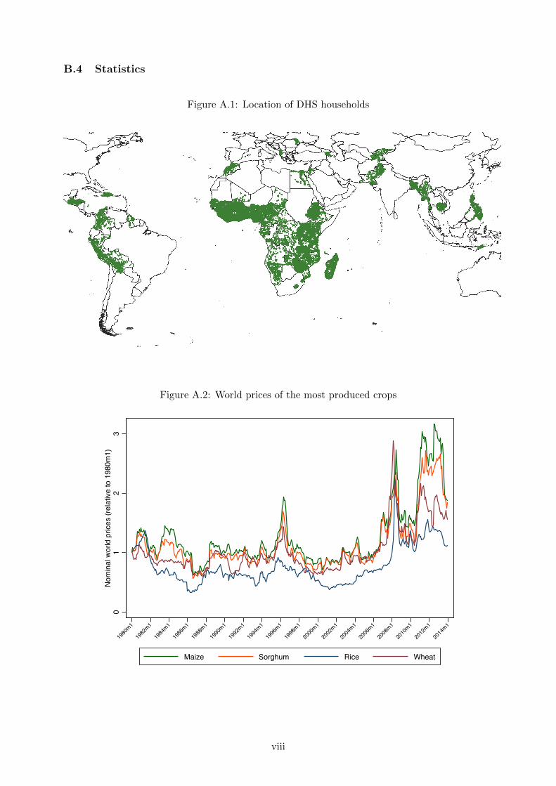
B.4 Statistics

Figure A.1: Location of DHS households

Figure A.2: World prices of the most produced crops

01

23

Nom

inal

wor

ld p

rices

(rel

ativ

e to

198

0m1)

1980

m1

1982

m1

1984

m1

1986

m1

1988

m1

1990

m1

1992

m1

1994

m1

1996

m1

1998

m1

2000

m1

2002

m1

2004

m1

2006

m1

2008

m1

2010

m1

2012

m1

2014

m1

Maize Sorghum Rice Wheat

viii

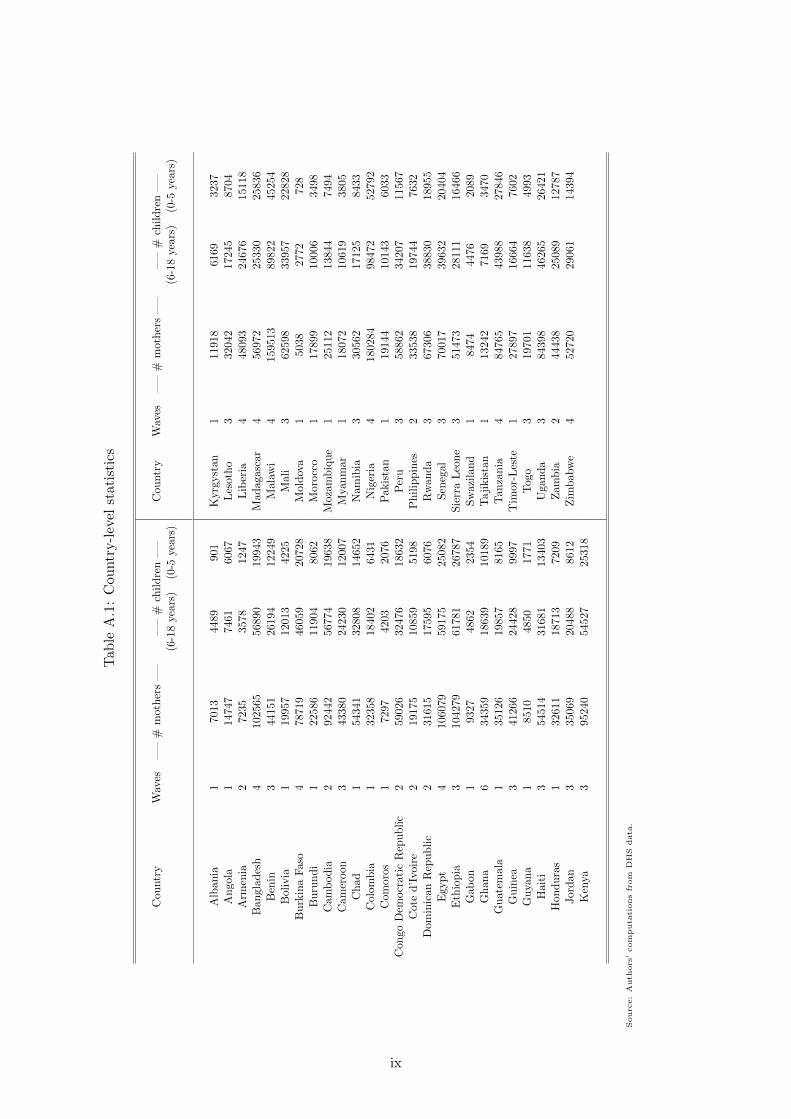
Tab

leA

.1:

Cou

ntr

y-l

evel

stat

isti

cs

Cou

ntr

yW

aves

—–

#m

oth

ers

—–

—–

#ch

ild

ren

—–

Cou

ntr

yW

aves

—–

#m

oth

ers

—–

—–

#ch

ild

ren

—–

(6-1

8yea

rs)

(0-5

year

s)(6

-18

yea

rs)

(0-5

year

s)

Alb

ania

170

1344

8990

1K

yrg

yst

an

111

918

616

9323

7A

ngol

a1

1474

774

6160

67L

esoth

o3

320

42

1724

587

04A

rmen

ia2

7235

3578

1247

Lib

eria

448

093

246

7615

118

Ban

glad

esh

410

2565

5689

019

943

Mad

agasc

ar

4569

72

2533

025

836

Ben

in3

4415

126

194

1224

9M

ala

wi

415

951

3898

22

452

54B

oliv

ia1

1995

712

013

4225

Mali

362

598

339

57

228

28

Bu

rkin

aF

aso

478

719

4605

920

728

Mold

ova

150

38

2772

728

Bu

run

di

122

586

1190

480

62M

orocc

o1

17899

100

06349

8C

amb

od

ia2

9244

256

774

1963

8M

ozam

biq

ue

125

112

13844

7494

Cam

eroon

343

380

2423

012

007

Mya

nm

ar

1180

72

1061

938

05C

had

154

341

3280

814

652

Nam

ibia

3305

6217

125

843

3C

olom

bia

132

358

1840

264

31N

iger

ia4

1802

84

984

7252

792

Com

oros

172

9742

0320

76P

akis

tan

1191

44

1014

360

33C

ongo

Dem

ocr

atic

Rep

ub

lic

259

026

3247

618

632

Per

u3

5886

234

207

11567

Cot

ed

’Ivoi

re2

1917

510

859

5198

Ph

ilip

pin

es2

3353

819

744

7632

Dom

inic

anR

epu

bli

c2

3161

517

595

6076

Rw

an

da

3673

06

3883

018

955

Egy

pt

410

6079

5917

525

082

Sen

egal

370

017

3963

220

404

Eth

iop

ia3

1042

7961

781

2678

7S

ierr

aL

eon

e3

51473

28111

16466

Gab

on1

9327

4862

2354

Sw

azil

an

d1

8474

447

6208

9G

han

a6

3435

918

639

1018

9T

aji

kis

tan

113

242

716

9347

0G

uat

emal

a1

3512

619

857

8165

Tan

zan

ia4

847

65

43988

2784

6G

uin

ea3

4126

624

428

9997

Tim

or-

Les

te1

278

97

166

64

760

2G

uya

na

185

1048

5017

71T

ogo

3197

01116

38

499

3H

aiti

354

514

3168

113

403

Ugan

da

384

398

462

65

264

21

Hon

du

ras

132

611

1871

372

09Z

am

bia

244

438

250

89

127

87

Jor

dan

335

069

2048

886

12Z

imb

abw

e4

5272

029

061

1439

4K

enya

395

240

5452

725

318

Sourc

e:

Auth

ors

’com

puta

tions

from

DH

Sdata

.

ix

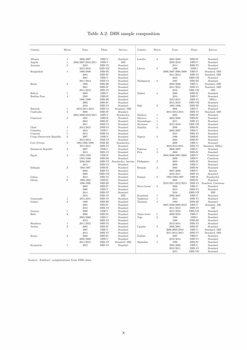
Table A.2: DHS sample composition

Country Waves Years Phase Surveys Country Waves Years Phase Surveys

Albania 1 2006/2007 DHS-V Standard Lesotho 3 2004/2005 DHS-IV StandardAngola 1 2006/2007-2010/2011 DHS-V MIS 2009/2010 DHS-V StandardArmenia 2 2010 DHS-VI Standard 2014 DHS-VI Standard

2015/2016 DHS-VII Standard Liberia 4 1986 DSH-I StandardBangladesh 4 1999/2000 DHS-III Standard 2006/2007-2008/2009 DHS-V Standard, MIS

2004 DHS-IV Standard 2011/2013 DHS-VI Standard, MIS2007 DHS-V Standard 2016 DHS-VII Standard

2011/2014 DSH-VI Standard Madagascar 4 1997 DHS-III StandardBenin 3 1996 DHS-III Standard 2008/2009 DHS-V Standard, MIS

2001 DHS-IV Standard 2011/2013 DHS-VI Standard, MIS2011/2012 DHS-VI Standard 2016 DHS-VII MIS

Bolivia 1 2008 DHS-V Standard Malawi 4 2000 DHS-IV StandardBurkina Faso 4 1993 DHS-II Standard 2010 DHS-V Standard

1998/1999 DHS-III Standard 2012-2014 DHS-VI MIS(s)2003 DHS-IV Standard 2015/2016 DHS-VII Standard2010 DHS-VI Standard Mali 3 1995/1996 DHS-III Standard

Burundi 1 2010/2011-2012 DHS-VI Standard, MIS 2006 DHS-V StandardCambodia 2 2000 DHS-IV Standard 2012/2013-2015 DHS-VI Standard, MIS

2005/2006-2010/2011 DHS-V Standard(s) Moldova 1 2005 DHS-IV StandardCameroon 3 1991 DHS-II Standard Morocco 1 2003/2004 DHS-IV Standard

2004 DHS-IV Standard Mozambique 1 2011 DHS-VI Standard2011 DSH-VI Standard Myanmar 1 2015/2016 DHS-VII Standard

Chad 1 2014/2015 DSH-VI Standard Namibia 3 2000 DHS-IV StandardColombia 1 2010 DSH-V Standard 2006/2007 DHS-V StandardComoros 1 2012 DSH-VI Standard 2013 DHS-VI StandardCongo Democratic Republic 2 2007 DSH-V Standard Nigeria 4 1990 DHS-II Standard

2013/2014 DSH-VI Standard 2003 DHS-IV StandardCote d’Ivoire 2 1994-1998/1999 DSH-III Standard(s) 2008 DHS-V Standard

2011-2012 DHS-VI Standard 2010-2013-2015 DHS-VI Standard, MIS(s)Dominican Republic 2 2007 DSH-V Standard Pakistan 1 2006/2007 DHS-V Standard

2013 DHS-VI Standard Peru 3 2000 DHS-IV StandardEgypt 4 1992/1993 DSH-II Standard 2003/2006-2007/2008 DHS-V Continous

1995/1996 DHS-III Standard 2009 DHS-V Continous2000-2005 DHS-VI Standard(s), Interim Philippines 2 2003 DHS-IV Standard

2014 DHS-VI Standard 2008 DHS-V StandardEthiopia 3 1992-1997 DSH-IV Standard Rwanda 3 2005 DHS-IV Standard

2003 DHS-VI Standard 2007/2008 DHS-V Interim2008 DHS-VII Standard 2010/2011 DHS-VI Standard

Gabon 1 2012 DHS-VI Standard Senegal 3 1992/1993-1997 DHS-II Standard(s)Ghana 6 1993-1994 DHS-II Standard 2005 DHS-IV Standard

1998-1999 DHS-III Standard 2010/2011-2012/2013 DHS-VI Standard, Continous2003 DHS-IV Standard Sierra Leone 3 2008 DHS-V Standard2008 DHS-V Standard 2013 DHS-VI Standard2014 DHS-VI Standard 2016 DHS-VII MIS2016 DHS-VI MIS Swaziland 1 2006/2007 DHS-V Standard

Guatemala 1 2014-2015 DHS-VI Standard Tajikistan 1 2012 DHS-VI StandardGuinea 3 1999 DHS-III Standard Tanzania 4 1999 DHS-III Standard

2005 DHS-IV Standard 2007/2008-2009/2010 DHS-V Standard, AIS2012 DHS-VI Standard 2011/2012 DHS-VI AIS

Guyana 1 2009 DSH-V Standard 2015/2016 DHS-VII StandardHaiti 3 2000 DHS-IV Standard Timor-Leste 1 2009/2010 DHS-V Standard

2005/2006 DHS-V Standard Togo 3 1988 DHS-I Standard2012 DHS-VI Standard 1998 DHS-III Standard

Honduras 1 2011/2012 DHS-VI Standard 2013/2014 DHS-VI StandardJordan 3 2002 DHS-IV Standard Uganda 3 2000/2001 DHS-IV Standard

2007 DHS-V Standard 2006-2009/2010 DHS-V Standard, MIS2012 DHS-VI Standard 2011-2014/2015 DHS-VI Standard, MIS

Kenya 3 2003 DHS-IV Standard Zambia 2 2007 DHS-V Standard2008/2009 DHS-V Standard 2013/2014 DHS-VI Standard2014/2015 DHS-VI Standard, MIS Zimbabwe 4 1999 DHS-IV Standard

Kyrgystan 1 2012 DHS-VI Standard 2005/2006 DHS-V Standard2010/2011 DHS-VI Standard

2015 DHS-VII Standard

Source: Authors’ computations from DHS data.

x

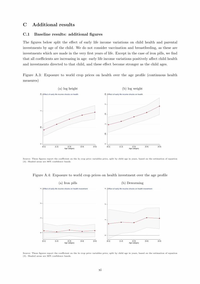
C Additional results

C.1 Baseline results: additional figures

The figures below split the effect of early life income variations on child health and parental

investments by age of the child. We do not consider vaccination and breastfeeding, as these are

investments which are made in the very first years of life. Except in the case of iron pills, we find

that all coefficients are increasing in age: early life income variations positively affect child health

and investments directed to that child, and these effect become stronger as the child ages.

Figure A.3: Exposure to world crop prices on health over the age profile (continuous health

measures)

(a) log height (b) log weight

0.0

5.1

.15

[0,1] [1,2] [2,3] [3,4] [4,5]Age category

Effect of early life income shocks on health

0.0

5.1

.15

.2.2

5

[0,1] [1,2] [2,3] [3,4] [4,5]Age category

Effect of early life income shocks on health

Source: These figures report the coefficient on the ln crop price variables price, split by child age in years, based on the estimation of equation

(3). Shaded areas are 90% confidence bands.

Figure A.4: Exposure to world crop prices on health investment over the age profile

(a) Iron pills (b) Deworming

0.1

.2.3

[0,1] [1,2] [2,3] [3,4] [4,5]Age category

Effect of early life income shocks on health investment

0.1

.2.3

[0,1] [1,2] [2,3] [3,4] [4,5]Age category

Effect of early life income shocks on health investment

Source: These figures report the coefficient on the ln crop price variables price, split by child age in years, based on the estimation of equation

(3). Shaded areas are 90% confidence bands.

xi

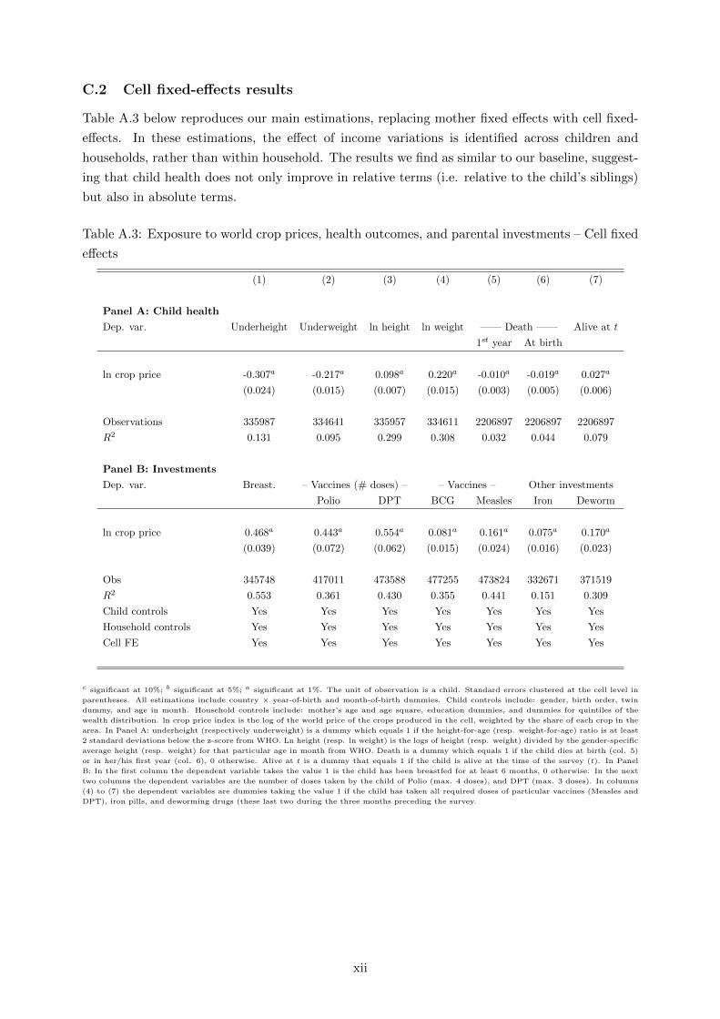
C.2 Cell fixed-effects results

Table A.3 below reproduces our main estimations, replacing mother fixed effects with cell fixed-

effects. In these estimations, the effect of income variations is identified across children and

households, rather than within household. The results we find as similar to our baseline, suggest-

ing that child health does not only improve in relative terms (i.e. relative to the child’s siblings)

but also in absolute terms.

Table A.3: Exposure to world crop prices, health outcomes, and parental investments – Cell fixed

effects

(1) (2) (3) (4) (5) (6) (7)

Panel A: Child health

Dep. var. Underheight Underweight ln height ln weight —— Death —— Alive at t

1st year At birth

ln crop price -0.307a -0.217a 0.098a 0.220a -0.010a -0.019a 0.027a

(0.024) (0.015) (0.007) (0.015) (0.003) (0.005) (0.006)

Observations 335987 334641 335957 334611 2206897 2206897 2206897

R2 0.131 0.095 0.299 0.308 0.032 0.044 0.079

Panel B: Investments

Dep. var. Breast. – Vaccines (# doses) – – Vaccines – Other investments

Polio DPT BCG Measles Iron Deworm

ln crop price 0.468a 0.443a 0.554a 0.081a 0.161a 0.075a 0.170a

(0.039) (0.072) (0.062) (0.015) (0.024) (0.016) (0.023)

Obs 345748 417011 473588 477255 473824 332671 371519

R2 0.553 0.361 0.430 0.355 0.441 0.151 0.309

Child controls Yes Yes Yes Yes Yes Yes Yes

Household controls Yes Yes Yes Yes Yes Yes Yes

Cell FE Yes Yes Yes Yes Yes Yes Yes

c significant at 10%; b significant at 5%; a significant at 1%. The unit of observation is a child. Standard errors clustered at the cell level in

parentheses. All estimations include country × year-of-birth and month-of-birth dummies. Child controls include: gender, birth order, twin

dummy, and age in month. Household controls include: mother’s age and age square, education dummies, and dummies for quintiles of the

wealth distribution. ln crop price index is the log of the world price of the crops produced in the cell, weighted by the share of each crop in the

area. In Panel A: underheight (respectively underweight) is a dummy which equals 1 if the height-for-age (resp. weight-for-age) ratio is at least

2 standard deviations below the z-score from WHO. Ln height (resp. ln weight) is the logs of height (resp. weight) divided by the gender-specific

average height (resp. weight) for that particular age in month from WHO. Death is a dummy which equals 1 if the child dies at birth (col. 5)

or in her/his first year (col. 6), 0 otherwise. Alive at t is a dummy that equals 1 if the child is alive at the time of the survey (t). In Panel

B: In the first column the dependent variable takes the value 1 is the child has been breastfed for at least 6 months, 0 otherwise. In the next

two columns the dependent variables are the number of doses taken by the child of Polio (max. 4 doses), and DPT (max. 3 doses). In columns

(4) to (7) the dependent variables are dummies taking the value 1 if the child has taken all required doses of particular vaccines (Measles and

DPT), iron pills, and deworming drugs (these last two during the three months preceding the survey.

xii

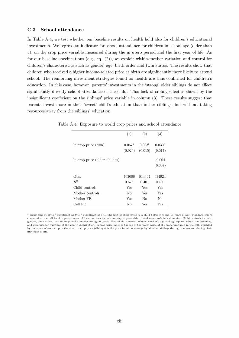
C.3 School attendance

In Table A.4, we test whether our baseline results on health hold also for children’s educational

investments. We regress an indicator for school attendance for children in school age (older than

5), on the crop price variable measured during the in utero period and the first year of life. As

for our baseline specifications (e.g., eq. (2)), we exploit within-mother variation and control for

children’s characteristics such as gender, age, birth order and twin status. The results show that

children who received a higher income-related price at birth are significantly more likely to attend

school. The reinforcing investment strategies found for health are thus confirmed for children’s

education. In this case, however, parents’ investments in the ‘strong’ older siblings do not affect

significantly directly school attendance of the child. This lack of sibling effect is shown by the

insignificant coefficient on the siblings’ price variable in column (3). These results suggest that

parents invest more in their ‘sweet’ child’s education than in her siblings, but without taking

resources away from the siblings’ education.

Table A.4: Exposure to world crop prices and school attendance

(1) (2) (3)

ln crop price (own) 0.067a 0.033b 0.030c

(0.020) (0.015) (0.017)

ln crop price (older siblings) -0.004

(0.007)

Obs. 763006 814394 634924

R2 0.676 0.401 0.400

Child controls Yes Yes Yes

Mother controls No Yes Yes

Mother FE Yes No No

Cell FE No Yes Yes

c significant at 10%; b significant at 5%; a significant at 1%. The unit of observation is a child between 6 and 17 years of age. Standard errors

clustered at the cell level in parentheses. All estimations include country × year-of-birth and month-of-birth dummies. Child controls include:

gender, birth order, twin dummy, and dummies for age in years. Household controls include: mother’s age and age square, education dummies,

and dummies for quintiles of the wealth distribution. ln crop price index is the log of the world price of the crops produced in the cell, weighted

by the share of each crop in the area. ln crop price (siblings) is the price faced on average by all elder siblings during in utero and during their

first year of life.

xiii

C.4 Child mortality and selection bias

Our results show a small and at times statistically significant effect of early life crop price varia-

tions on mortality at birth and in the first year of life, and on survival later on. In this section we

examine whether this selective mortality affects our baseline results on child health and parental

investments in child health. More precisely, we try to account for a potential selection bias by

including a selection correction term in our estimations. Given the structure of our selection

equation (which includes two high dimensional sets of fixed effects), we cannot use probit or

other maximum likelihood estimators to implement a standard Heckman procedure. The vari-

ables being the same in our baseline equations and in the selection equation, we have to rely on

some nonlinear transformation of the predicted probabilities to correct for selection. We follow

Cosslett (1991), who proposes a semi-parametric estimator in which the selection correction is

approximated through indicator variables computed from the predictions obtained from survival

regression. In Tables A.5 and A.6, we include in our baseline specifications dummies for 100

bins corresponding to each centile of the predicted survival probabilities as correction terms. The

survival probabilities are computed from the specification in Panel A, column (7) of Tables 2 and

4 (for the sibling regressions). For both child health and parental investments, the estimated

coefficients on the price index variable specific to the child are very close from the benchmark

ones. We have also tried, as an alternative methodology, to weight our estimation by survival

probabilities; the results were similar.

xiv

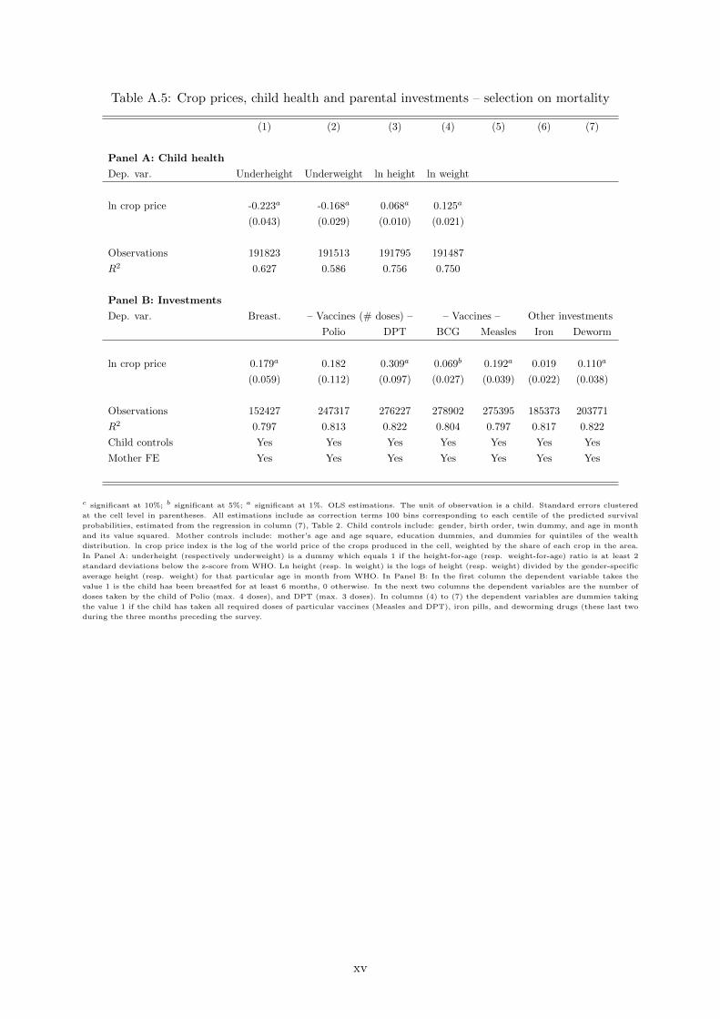
Table A.5: Crop prices, child health and parental investments – selection on mortality

(1) (2) (3) (4) (5) (6) (7)

Panel A: Child health

Dep. var. Underheight Underweight ln height ln weight

ln crop price -0.223a -0.168a 0.068a 0.125a

(0.043) (0.029) (0.010) (0.021)

Observations 191823 191513 191795 191487

R2 0.627 0.586 0.756 0.750

Panel B: Investments

Dep. var. Breast. – Vaccines (# doses) – – Vaccines – Other investments

Polio DPT BCG Measles Iron Deworm

ln crop price 0.179a 0.182 0.309a 0.069b 0.192a 0.019 0.110a

(0.059) (0.112) (0.097) (0.027) (0.039) (0.022) (0.038)

Observations 152427 247317 276227 278902 275395 185373 203771

R2 0.797 0.813 0.822 0.804 0.797 0.817 0.822

Child controls Yes Yes Yes Yes Yes Yes Yes

Mother FE Yes Yes Yes Yes Yes Yes Yes

c significant at 10%; b significant at 5%; a significant at 1%. OLS estimations. The unit of observation is a child. Standard errors clustered

at the cell level in parentheses. All estimations include as correction terms 100 bins corresponding to each centile of the predicted survival

probabilities, estimated from the regression in column (7), Table 2. Child controls include: gender, birth order, twin dummy, and age in month

and its value squared. Mother controls include: mother’s age and age square, education dummies, and dummies for quintiles of the wealth

distribution. ln crop price index is the log of the world price of the crops produced in the cell, weighted by the share of each crop in the area.

In Panel A: underheight (respectively underweight) is a dummy which equals 1 if the height-for-age (resp. weight-for-age) ratio is at least 2

standard deviations below the z-score from WHO. Ln height (resp. ln weight) is the logs of height (resp. weight) divided by the gender-specific

average height (resp. weight) for that particular age in month from WHO. In Panel B: In the first column the dependent variable takes the

value 1 is the child has been breastfed for at least 6 months, 0 otherwise. In the next two columns the dependent variables are the number of

doses taken by the child of Polio (max. 4 doses), and DPT (max. 3 doses). In columns (4) to (7) the dependent variables are dummies taking

the value 1 if the child has taken all required doses of particular vaccines (Measles and DPT), iron pills, and deworming drugs (these last two

during the three months preceding the survey.

xv

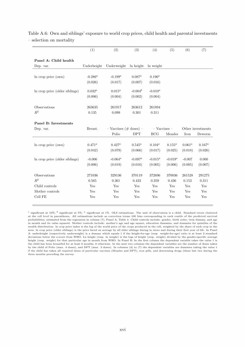
Table A.6: Own and siblings’ exposure to world crop prices, child health and parental investments

– selection on mortality

(1) (2) (3) (4) (5) (6) (7)

Panel A: Child health

Dep. var. Underheight Underweight ln height ln weight

ln crop price (own) -0.286a -0.199a 0.087a 0.196a

(0.026) (0.017) (0.007) (0.016)

ln crop price (older siblings) 0.032a 0.015a -0.004b -0.010a

(0.006) (0.004) (0.002) (0.004)

Observations 263635 261917 263612 261894

R2 0.135 0.099 0.301 0.311

Panel B: Investments

Dep. var. Breast. – Vaccines (# doses) – – Vaccines – Other investments

Polio DPT BCG Measles Iron Deworm

ln crop price (own) 0.471a 0.427a 0.545a 0.104a 0.155a 0.061a 0.167a

(0.042) (0.079) (0.066) (0.017) (0.025) (0.018) (0.026)

ln crop price (older siblings) -0.006 -0.064a -0.097a -0.015a -0.019a -0.007 0.000

(0.006) (0.019) (0.016) (0.005) (0.006) (0.005) (0.007)

Observations 271036 329136 370119 372696 370036 261528 291275

R2 0.565 0.361 0.433 0.359 0.436 0.153 0.311

Child controls Yes Yes Yes Yes Yes Yes Yes

Mother controls Yes Yes Yes Yes Yes Yes Yes

Cell FE Yes Yes Yes Yes Yes Yes Yes

c significant at 10%; b significant at 5%; a significant at 1%. OLS estimations. The unit of observation is a child. Standard errors clustered

at the cell level in parentheses. All estimations include as correction terms 100 bins corresponding to each centile of the predicted survival

probabilities, estimated from the regression in column (7), Panel A, Table 4. Child controls include: gender, birth order, twin dummy, and age

in month and its value squared. Mother controls include: mother’s age and age square, education dummies, and dummies for quintiles of the

wealth distribution. ln crop price index is the log of the world price of the crops produced in the cell, weighted by the share of each crop in the

area. ln crop price (older siblings) is the price faced on average by all elder siblings during in utero and during their first year of life. In Panel

A: underheight (respectively underweight) is a dummy which equals 1 if the height-for-age (resp. weight-for-age) ratio is at least 2 standard

deviations below the z-score from WHO. Ln height (resp. ln weight) is the logs of height (resp. weight) divided by the gender-specific average

height (resp. weight) for that particular age in month from WHO. In Panel B: In the first column the dependent variable takes the value 1 is

the child has been breastfed for at least 6 months, 0 otherwise. In the next two columns the dependent variables are the number of doses taken

by the child of Polio (max. 4 doses), and DPT (max. 3 doses). In columns (4) to (7) the dependent variables are dummies taking the value 1

if the child has taken all required doses of particular vaccines (Measles and DPT), iron pills, and deworming drugs (these last two during the

three months preceding the survey.

xvi

C.5 Robustness: full sequence of prices

Price are persistent over time. This persistence is an issue in our case, as it implies that we might

be capturing the effect of prices in subsequent years on subsequent health and not the effect of

early life prices on subsequent health. To solve this issue, we can include the full sequence of

prices in our estimations, i.e. control for the prices observed when the child is 2, 3 or 4 years

old.19 Equation (2) becomes:

Yc = α logP c,k +

4∑a=2

[βa1 log Pak + βa2 ln P

ak × Iak ] + D′cδ + µH + γi,t + νm + εc (12)

Equation (12) includes the full sequence of prices Pak for children in their second, third and

fourth years. Because not all children reached that age, we interact Pak with an indicator variable

which equal 1 if child k is aged a or more. The set of coefficient βa2 represents effect of prices

variations in later life. βa1 , on the other hand, should generally be insignificant.

The results on health are shown in Table A.7, while those on health investments are in Table

A.8. Four elements are worth mentioning. First, prices during pregnancy and first year remain

significant and keep the same signs as in the baseline estimations, which means we were not

picking up the effect of price persistence. Second, prices during pregnancy and in the first year

have quantitatively similar effects, thereby supporting the choice of lumping them together in

a single price variable. Third, prices in later years, while being generally significant, have a

quantitatively much more limited impact on health indicators. Fourth, the non interacted prices

are in most cases insignificant, which is in line with expectations.

Finally, in Figure A.5 we show that the results on the effect of early life price variations on

health and health investment over time are robust to the inclusion of the full sequence of prices.

19Note that in our empirical specification the mother fixed effects de facto absorb the effect of prices at the timeof the survey. The estimates in specification (12) are thus relative to this benchmark prices at the year of thesurvey.

xvii

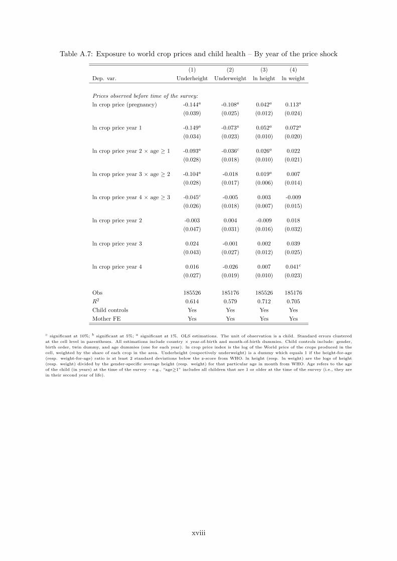
Table A.7: Exposure to world crop prices and child health – By year of the price shock

(1) (2) (3) (4)

Dep. var. Underheight Underweight ln height ln weight

Prices observed before time of the survey:

ln crop price (pregnancy) -0.144a -0.108a 0.042a 0.113a

(0.039) (0.025) (0.012) (0.024)

ln crop price year 1 -0.149a -0.073a 0.052a 0.072a

(0.034) (0.023) (0.010) (0.020)

ln crop price year 2 × age ≥ 1 -0.093a -0.036c 0.026a 0.022

(0.028) (0.018) (0.010) (0.021)

ln crop price year 3 × age ≥ 2 -0.104a -0.018 0.019a 0.007

(0.028) (0.017) (0.006) (0.014)

ln crop price year 4 × age ≥ 3 -0.045c -0.005 0.003 -0.009

(0.026) (0.018) (0.007) (0.015)

ln crop price year 2 -0.003 0.004 -0.009 0.018

(0.047) (0.031) (0.016) (0.032)

ln crop price year 3 0.024 -0.001 0.002 0.039

(0.043) (0.027) (0.012) (0.025)

ln crop price year 4 0.016 -0.026 0.007 0.041c

(0.027) (0.019) (0.010) (0.023)

Obs 185526 185176 185526 185176

R2 0.614 0.579 0.712 0.705

Child controls Yes Yes Yes Yes

Mother FE Yes Yes Yes Yes

c significant at 10%; b significant at 5%; a significant at 1%. OLS estimations. The unit of observation is a child. Standard errors clustered

at the cell level in parentheses. All estimations include country × year-of-birth and month-of-birth dummies. Child controls include: gender,

birth order, twin dummy, and age dummies (one for each year). ln crop price index is the log of the World price of the crops produced in the

cell, weighted by the share of each crop in the area. Underheight (respectively underweight) is a dummy which equals 1 if the height-for-age

(resp. weight-for-age) ratio is at least 2 standard deviations below the z-score from WHO. ln height (resp. ln weight) are the logs of height

(resp. weight) divided by the gender-specific average height (resp. weight) for that particular age in month from WHO. Age refers to the age

of the child (in years) at the time of the survey – e.g., “age≥1” includes all children that are 1 or older at the time of the survey (i.e., they are

in their second year of life).

xviii

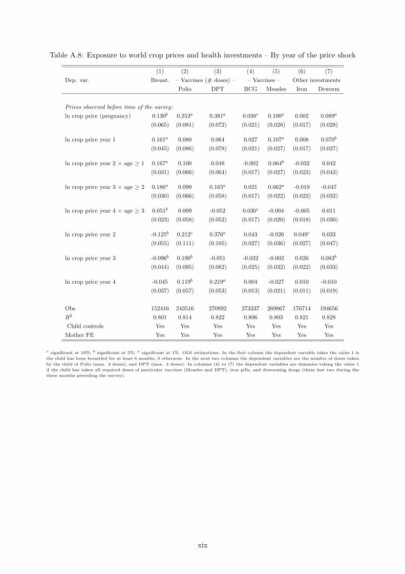
Table A.8: Exposure to world crop prices and health investments – By year of the price shock

(1) (2) (3) (4) (5) (6) (7)

Dep. var. Breast. – Vaccines (# doses) – – Vaccines – Other investments

Polio DPT BCG Measles Iron Deworm

Prices observed before time of the survey:

ln crop price (pregnancy) 0.130b 0.252a 0.381a 0.038c 0.100a 0.002 0.089a

(0.065) (0.081) (0.072) (0.021) (0.028) (0.017) (0.028)

ln crop price year 1 0.161a 0.080 0.064 0.027 0.107a 0.008 0.070b

(0.045) (0.086) (0.078) (0.021) (0.027) (0.017) (0.027)

ln crop price year 2 × age ≥ 1 0.167a 0.100 0.048 -0.002 0.064b -0.032 0.042

(0.031) (0.066) (0.064) (0.017) (0.027) (0.023) (0.043)

ln crop price year 3 × age ≥ 2 0.186a 0.099 0.165a 0.021 0.062a -0.019 -0.047

(0.030) (0.066) (0.058) (0.017) (0.022) (0.022) (0.032)

ln crop price year 4 × age ≥ 3 0.051b 0.009 -0.052 0.030c -0.004 -0.005 0.011

(0.023) (0.058) (0.052) (0.017) (0.020) (0.018) (0.030)

ln crop price year 2 -0.125b 0.212c 0.376a 0.043 -0.026 0.049c 0.033

(0.055) (0.111) (0.105) (0.027) (0.036) (0.027) (0.047)

ln crop price year 3 -0.096b 0.190b -0.051 -0.032 -0.002 0.026 0.083b

(0.044) (0.095) (0.082) (0.025) (0.032) (0.022) (0.033)

ln crop price year 4 -0.045 0.119b 0.219a 0.004 -0.027 0.010 -0.010

(0.037) (0.057) (0.053) (0.013) (0.021) (0.011) (0.019)

Obs 152416 243516 270892 273337 269867 176714 194656

R2 0.801 0.814 0.822 0.806 0.803 0.821 0.828

Child controls Yes Yes Yes Yes Yes Yes Yes

Mother FE Yes Yes Yes Yes Yes Yes Yes

c significant at 10%; b significant at 5%; a significant at 1%. OLS estimations. In the first column the dependent variable takes the value 1 is

the child has been breastfed for at least 6 months, 0 otherwise. In the next two columns the dependent variables are the number of doses taken

by the child of Polio (max. 4 doses), and DPT (max. 3 doses). In columns (4) to (7) the dependent variables are dummies taking the value 1

if the child has taken all required doses of particular vaccines (Measles and DPT), iron pills, and deworming drugs (these last two during the

three months preceding the survey).

xix

Figure A.5: Income, child health and parental investments over the age profile (full price sequence)

(a) Underheight (b) Underweight

−.4

−.3

−.2

−.1

0

[0,1] [1,2] [2,3] [3,4] [4,5]Age category

Effect of early life income shocks on health

−.2

5−

.2−

.15

−.1

−.0

50

[0,1] [1,2] [2,3] [3,4] [4,5]Age category

Effect of early life income shocks on health

(c) log height (d) log weight

0.0

2.0

4.0

6.0

8.1

[0,1] [1,2] [2,3] [3,4] [4,5]Age category

Effect of early life income shocks on health

0.0

5.1

.15

.2

[0,1] [1,2] [2,3] [3,4] [4,5]Age category

Effect of early life income shocks on health

(e) Iron pills (f) Deworming

0.1

.2.3

[0,1] [1,2] [2,3] [3,4] [4,5]Age category

Effect of early life income shocks on health investment

0.1

.2.3

[0,1] [1,2] [2,3] [3,4] [4,5]Age category

Effect of early life income shocks on health investment

Source: These figures report the coefficient on the ln crop price variables price, split by child age in years, based on the estimation of equation

(3), but including the full sequence of later life prices as in equation (12). Shaded areas are 90% confidence bands.

xx

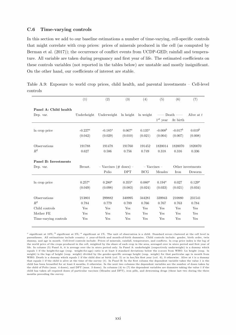
C.6 Time-varying controls

In this section we add to our baseline estimations a number of time-varying, cell-specific controls

that might correlate with crop prices: prices of minerals produced in the cell (as computed by

Berman et al. (2017)); the occurrence of conflict events from UCDP-GED; rainfall and tempera-

ture. All variable are taken during pregnancy and first year of life. The estimated coefficients on

these controls variables (not reported in the tables below) are unstable and mostly insignificant.

On the other hand, our coefficients of interest are stable.

Table A.9: Exposure to world crop prices, child health, and parental investments – Cell-level

controls

(1) (2) (3) (4) (5) (6) (7)

Panel A: Child health

Dep. var. Underheight Underweight ln height ln weight —— Death —— Alive at t

1st year At birth

ln crop price -0.227a -0.185a 0.067a 0.135a -0.008b -0.017b 0.019b

(0.042) (0.029) (0.010) (0.021) (0.004) (0.007) (0.008)

Observations 191788 191478 191760 191452 1820014 1820070 1820070

R2 0.627 0.586 0.756 0.749 0.318 0.316 0.336

Panel B: Investments

Dep. var. Breast. – Vaccines (# doses) – – Vaccines – Other investments

Polio DPT BCG Measles Iron Deworm

ln crop price 0.257a 0.280a 0.355a 0.080a 0.194a 0.027 0.129a

(0.049) (0.098) (0.083) (0.024) (0.033) (0.021) (0.034)

Observations 213801 299882 340995 344281 339943 210880 231541

R2 0.784 0.779 0.789 0.766 0.767 0.763 0.784

Child controls Yes Yes Yes Yes Yes Yes Yes

Mother FE Yes Yes Yes Yes Yes Yes Yes

Time-varying controls Yes Yes Yes Yes Yes Yes Yes

c significant at 10%; b significant at 5%; a significant at 1%. The unit of observation is a child. Standard errors clustered at the cell level in

parentheses. All estimations include country × year-of-birth and month-of-birth dummies. Child controls include: gender, birth order, twin

dummy, and age in month. Cell-level controls include: Prices of minerals, rainfall, temperature, and conflicts. ln crop price index is the log of

the world price of the crops produced in the cell, weighted by the share of each crop in the area, averaged over in utero period and first year of

life. In column (5) Panel A, it is average over the in utero period only. In Panel A: underheight (respectively underweight) is a dummy which

equals 1 if the height-for-age (resp. weight-for-age) ratio is at least 2 standard deviations below the z-score from WHO. Ln height (resp. ln

weight) is the logs of height (resp. weight) divided by the gender-specific average height (resp. weight) for that particular age in month from

WHO. Death is a dummy which equals 1 if the child dies at birth (col. 5) or in her/his first year (col. 6), 0 otherwise. Alive at t is a dummy

that equals 1 if the child is alive at the time of the survey (t). In Panel B: In the first column the dependent variable takes the value 1 is the

child has been breastfed for at least 6 months, 0 otherwise. In the next two columns the dependent variables are the number of doses taken by

the child of Polio (max. 4 doses), and DPT (max. 3 doses). In columns (4) to (7) the dependent variables are dummies taking the value 1 if the

child has taken all required doses of particular vaccines (Measles and DPT), iron pills, and deworming drugs (these last two during the three

months preceding the survey.

xxi

Table A.10: Own and siblings’ exposure to world crop prices, child health, and parental invest-

ments – cell-level controls

(1) (2) (3) (4) (5) (6) (7)

Panel A: Child health

Dep. var. Underheight Underweight ln height ln weight —— Death —— Alive at t

1st year At birth

ln crop price (own) -0.302a -0.205a 0.090a 0.198a -0.010a -0.012b 0.011

(0.025) (0.017) (0.007) (0.015) (0.003) (0.006) (0.007)

ln crop price (older siblings) 0.032a 0.013a -0.004b -0.009a 0.001 0.002 -0.009a

(0.006) (0.004) (0.001) (0.003) (0.002) (0.002) (0.003)

Observations 191788 191478 191760 191452 1820014 1820070 1820070

R2 0.627 0.586 0.756 0.749 0.318 0.316 0.336

Panel B: Investments

Dep. var. Breast. – Vaccines (# doses) – – Vaccines – Other investments

Polio DPT BCG Measles Iron Deworm

ln crop price (own) 0.469a 0.423a 0.542a 0.091a 0.166a 0.073a 0.187a

(0.041) (0.077) (0.064) (0.017) (0.025) (0.017) (0.025)

ln crop price (older siblings) -0.005 -0.062a -0.092a -0.011b -0.020a -0.010b -0.003

(0.005) (0.018) (0.015) (0.005) (0.005) (0.005) (0.006)

Observations 271008 329107 370085 372663 370002 261496 291246

R2 0.565 0.361 0.432 0.358 0.435 0.152 0.311

Child controls Yes Yes Yes Yes Yes Yes Yes

Household controls Yes Yes Yes Yes Yes Yes Yes

Cell FE Yes Yes Yes Yes Yes Yes Yes

Time-varying controls Yes Yes Yes Yes Yes Yes Yes

c significant at 10%; b significant at 5%; a significant at 1%. The unit of observation is a child. Standard errors clustered at the cell level in

parentheses. All estimations include country × year-of-birth and month-of-birth dummies. Child controls include: gender, birth order, twin

dummy, and age in month. Cell-level controls include: Prices of minerals, rainfall, temperature, and conflicts. ln crop price index is the log of

the world price of the crops produced in the cell, weighted by the share of each crop in the area, averaged over in utero period and first year of

life. In column (5) Panel A, it is average over the in utero period only. In Panel A: underheight (respectively underweight) is a dummy which

equals 1 if the height-for-age (resp. weight-for-age) ratio is at least 2 standard deviations below the z-score from WHO. Ln height (resp. ln

weight) is the logs of height (resp. weight) divided by the gender-specific average height (resp. weight) for that particular age in month from

WHO. Death is a dummy which equals 1 if the child dies at birth (col. 5) or in her/his first year (col. 6), 0 otherwise. Alive at t is a dummy

that equals 1 if the child is alive at the time of the survey (t). In Panel B: In the first column the dependent variable takes the value 1 is the

child has been breastfed for at least 6 months, 0 otherwise. In the next two columns the dependent variables are the number of doses taken by

the child of Polio (max. 4 doses), and DPT (max. 3 doses). In columns (4) to (7) the dependent variables are dummies taking the value 1 if the

child has taken all required doses of particular vaccines (Measles and DPT), iron pills, and deworming drugs (these last two during the three

months preceding the survey.

xxii

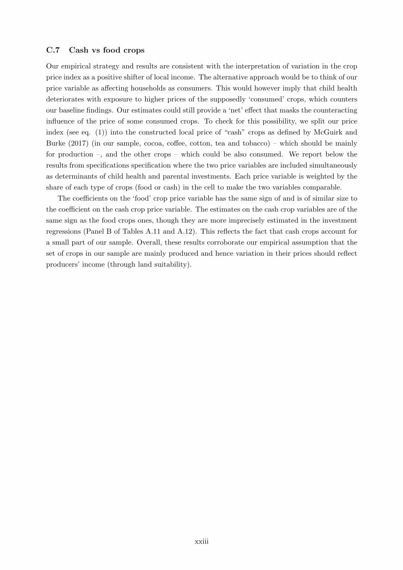
C.7 Cash vs food crops

Our empirical strategy and results are consistent with the interpretation of variation in the crop

price index as a positive shifter of local income. The alternative approach would be to think of our

price variable as affecting households as consumers. This would however imply that child health

deteriorates with exposure to higher prices of the supposedly ‘consumed’ crops, which counters

our baseline findings. Our estimates could still provide a ‘net’ effect that masks the counteracting

influence of the price of some consumed crops. To check for this possibility, we split our price

index (see eq. (1)) into the constructed local price of “cash” crops as defined by McGuirk and

Burke (2017) (in our sample, cocoa, coffee, cotton, tea and tobacco) – which should be mainly

for production –, and the other crops – which could be also consumed. We report below the

results from specifications specification where the two price variables are included simultaneously

as determinants of child health and parental investments. Each price variable is weighted by the

share of each type of crops (food or cash) in the cell to make the two variables comparable.

The coefficients on the ‘food’ crop price variable has the same sign of and is of similar size to

the coefficient on the cash crop price variable. The estimates on the cash crop variables are of the

same sign as the food crops ones, though they are more imprecisely estimated in the investment

regressions (Panel B of Tables A.11 and A.12). This reflects the fact that cash crops account for

a small part of our sample. Overall, these results corroborate our empirical assumption that the

set of crops in our sample are mainly produced and hence variation in their prices should reflect

producers’ income (through land suitability).

xxiii

Table A.11: Exposure to world crop prices, child health and parental investments – ‘Cash’ vs.

‘food’ crops

(1) (2) (3) (4) (5) (6) (7)

Panel A: Child health

Dep. var. Underheight Underweight ln height ln weight —— Death —— Alive at t

1st year At birth

ln crop price (food) -0.247a -0.198a 0.065a 0.122a -0.006 -0.016b 0.025a

(0.045) (0.031) (0.011) (0.022) (0.004) (0.007) (0.009)

ln crop price (cash) -0.197a -0.145a 0.072a 0.134a -0.011c -0.026a 0.028b

(0.064) (0.046) (0.015) (0.033) (0.006) (0.009) (0.012)

Observations 184675 184345 184647 184319 2183982 2183982 2183982

R2 0.627 0.586 0.755 0.747 0.281 0.281 0.305

Panel B: Investments

Dep. var. Breast. – Vaccines (# doses) – – Vaccines – Other investments

Polio DPT BCG Measles Iron Deworm

ln crop price (food) 0.238a 0.229c 0.383a 0.092a 0.227a 0.012 0.143a

(0.065) (0.120) (0.106) (0.029) (0.043) (0.024) (0.041)

ln crop price (cash) 0.011 0.129 0.061 0.018 0.111c 0.006 0.009

(0.091) (0.164) (0.145) (0.043) (0.060) (0.031) (0.057)

Obs 145877 240171 267018 269561 266136 182288 200470

R2 0.799 0.812 0.820 0.804 0.796 0.818 0.822

Child controls Yes Yes Yes Yes Yes Yes Yes

Mother FE Yes Yes Yes Yes Yes Yes Yes

c significant at 10%; b significant at 5%; a significant at 1%. The unit of observation is a child. Standard errors clustered at the cell level in

parentheses. All estimations include country × year-of-birth and month-of-birth dummies. Child controls include: gender, birth order, twin

dummy, and age in month. ln crop price index is the log of the world price of the crops produced in the cell, weighted by the share of each crop

in the area. In Panel A: underheight (respectively underweight) is a dummy which equals 1 if the height-for-age (resp. weight-for-age) ratio

is at least 2 standard deviations below the z-score from WHO. Ln height (resp. ln weight) is the logs of height (resp. weight) divided by the

gender-specific average height (resp. weight) for that particular age in month from WHO. Death is a dummy which equals 1 if the child dies at

birth (col. 5) or in her/his first year (col. 6), 0 otherwise. Alive at t is a dummy that equals 1 if the child is alive at the time of the survey (t).

In Panel B: In the first column the dependent variable takes the value 1 is the child has been breastfed for at least 6 months, 0 otherwise. In

the next two columns the dependent variables are the number of doses taken by the child of Polio (max. 4 doses), and DPT (max. 3 doses).

In columns (4) to (7) the dependent variables are dummies taking the value 1 if the child has taken all required doses of particular vaccines

(Measles and DPT), iron pills, and deworming drugs (these last two during the three months preceding the survey.

xxiv

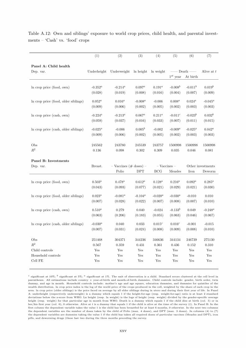
Table A.12: Own and siblings’ exposure to world crop prices, child health, and parental invest-

ments – ‘Cash’ vs. ‘food’ crops

(1) (2) (3) (4) (5) (6) (7)

Panel A: Child health

Dep. var. Underheight Underweight ln height ln weight —— Death —— Alive at t

1st year At birth

ln crop price (food, own) -0.352a -0.214a 0.097a 0.191a -0.008b -0.011b 0.019b

(0.028) (0.019) (0.008) (0.016) (0.004) (0.007) (0.009)

ln crop price (food, older siblings) 0.052a 0.016a -0.008a -0.006 0.008a 0.024a -0.045a

(0.009) (0.006) (0.002) (0.005) (0.002) (0.003) (0.003)

ln crop price (cash, own) -0.224a -0.213a 0.067a 0.211a -0.011c -0.023b 0.032b

(0.059) (0.037) (0.016) (0.033) (0.007) (0.011) (0.015)

ln crop price (cash, older siblings) -0.025a -0.006 0.005b -0.002 -0.009a -0.025a 0.042a

(0.009) (0.006) (0.002) (0.005) (0.002) (0.003) (0.003)

Obs 245562 243780 245539 243757 1500998 1500998 1500998

R2 0.136 0.098 0.302 0.309 0.035 0.046 0.081

Panel B: Investments

Dep. var. Breast. – Vaccines (# doses) – – Vaccines – Other investments

Polio DPT BCG Measles Iron Deworm

ln crop price (food, own) 0.503a 0.478a 0.612a 0.128a 0.216a 0.092a 0.285a

(0.043) (0.093) (0.077) (0.021) (0.029) (0.021) (0.030)

ln crop price (food, older siblings) 0.023a -0.081a -0.104a -0.020a -0.030a -0.010 0.010

(0.007) (0.028) (0.022) (0.007) (0.008) (0.007) (0.010)

ln crop price (cash, own) 0.510a 0.279 0.040 -0.024 -0.133b 0.049 -0.248a

(0.063) (0.206) (0.183) (0.055) (0.063) (0.046) (0.067)

ln crop price (cash, older siblings) -0.030a 0.040 0.033 0.015c 0.016c -0.001 -0.015

(0.007) (0.031) (0.024) (0.008) (0.009) (0.008) (0.010)

Obs 251468 304371 344236 346636 344134 246739 275130

R2 0.567 0.359 0.431 0.361 0.436 0.152 0.310

Child controls Yes Yes Yes Yes Yes Yes Yes

Household controls Yes Yes Yes Yes Yes Yes Yes

Cell FE Yes Yes Yes Yes Yes Yes Yes

c significant at 10%; b significant at 5%; a significant at 1%. The unit of observation is a child. Standard errors clustered at the cell level in

parentheses. All estimations include country × year-of-birth and month-of-birth dummies. Child controls include: gender, birth order, twin

dummy, and age in month. Household controls include: mother’s age and age square, education dummies, and dummies for quintiles of the

wealth distribution. ln crop price index is the log of the world price of the crops produced in the cell, weighted by the share of each crop in the

area. ln crop price (older siblings) is the price faced on average by all elder siblings during in utero and during their first year of life. In Panel

A: underheight (respectively underweight) is a dummy which equals 1 if the height-for-age (resp. weight-for-age) ratio is at least 2 standard

deviations below the z-score from WHO. Ln height (resp. ln weight) is the logs of height (resp. weight) divided by the gender-specific average

height (resp. weight) for that particular age in month from WHO. Death is a dummy which equals 1 if the child dies at birth (col. 5) or in

her/his first year (col. 6), 0 otherwise. Alive at t is a dummy that equals 1 if the child is alive at the time of the survey (t). In Panel B: In the

first column the dependent variable takes the value 1 is the child has been breastfed for at least 6 months, 0 otherwise. In the next two columns

the dependent variables are the number of doses taken by the child of Polio (max. 4 doses), and DPT (max. 3 doses). In columns (4) to (7)

the dependent variables are dummies taking the value 1 if the child has taken all required doses of particular vaccines (Measles and DPT), iron

pills, and deworming drugs (these last two during the three months preceding the survey.

xxv

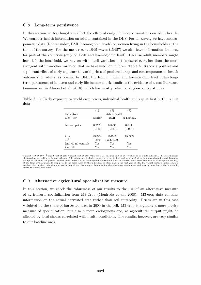
C.8 Long-term persistence

In this section we test long-term effect the effect of early life income variations on adult health.

We consider health information on adults contained in the DHS. For all waves, we have anthro-

pometric data (Rohrer index, BMI, haemoglobin levels) on women living in the households at the

time of the survey. For the most recent DHS waves (DHS7) we also have information for men,

for part of the countries (only on BMI and haemoglobin level). Because adult members might

have left the household, we rely on within-cell variation in this exercise, rather than the more

stringent within-mother variation that we have used for children. Table A.13 show a positive and

significant effect of early exposure to world prices of produced crops and contemporaneous health

outcomes for adults, as proxied by BMI, the Rohrer index, and haemoglobin level. This long-

term persistence of in-utero and early life income shocks confirms the evidence of a vast literature

(summarised in Almond et al., 2018), which has mostly relied on single-country studies.

Table A.13: Early exposure to world crop prices, individual health and age at first birth – adultdata

(1) (2) (3)Indicators ——— Adult health ———Dep. var. Rohrer BMI ln hemogl.

ln crop price 0.252b 0.829a 0.044a

(0.119) (0.123) (0.007)

Obs. 238954 257965 150969R2 0.272 0.306 0.299Individual controls Yes Yes YesCell FE Yes Yes Yes

c significant at 10%; b significant at 5%; a significant at 1%. OLS estimations. The unit of observation is an adult individual. Standard errorsclustered at the cell level in parentheses. All estimations include country × year-of-birth and month-of-birth dummies dummies and dummiesfor age of the adult (in years). Rohrer index, BMI, and ln haemoglobin are the individual’s Rohrer index, BMI and level of haemoglobin (in log)at the time of the survey. ln crop price is the price faced by the individual in utero and in the first year of life. Individual controls include child’sgender, birth order, twin dummy, age in month and its square, dummies for the education attainment and wealth quintiles of the householdwhere the household lives.

C.9 Alternative agricultural specialization measure

In this section, we check the robustness of our results to the use of an alternative measure

of agricultural specialization from M3-Crop (Monfreda et al., 2008). M3-crop data contains

information on the actual harvested area rather than soil suitability. Prices are in this case

weighted by the share of harvested area in 2000 in the cell. M3 crop is arguably a more precise

measure of specialization, but also a more endogenous one, as agricultural output might be

affected by local shocks correlated with health conditions. The results, however, are very similar

to our baseline ones.

xxvi

Table A.14: Exposure to world crop prices, child health, and health investments – M3 crop data

(1) (2) (3) (4) (5) (6) (7)

Panel A: Child health

Dep. var. Underheight Underweight ln height ln weight —— Death —— Alive at t

1st year At birth

ln crop price -0.122a -0.101a 0.035a 0.076a -0.005c -0.013a 0.010c

(0.030) (0.022) (0.007) (0.015) (0.002) (0.004) (0.005)

Observations 193256 192907 193228 192881 2262596 2262596 2262596

R2 0.627 0.586 0.756 0.750 0.281 0.281 0.305

Panel B: Investments

Dep. var. Breast. – Vaccines (# doses) – – Vaccines – Other investments

Polio DPT BCG Measles Iron Deworm

ln crop price 0.178a 0.187b 0.272a 0.052b 0.128a 0.015 0.044c

(0.042) (0.078) (0.070) (0.020) (0.028) (0.015) (0.026)

Obs 153790 246654 277090 279729 276272 183213 201795

R2 0.797 0.814 0.822 0.804 0.797 0.816 0.822

Child controls Yes Yes Yes Yes Yes Yes Yes

Mother FE Yes Yes Yes Yes Yes Yes Yes

c significant at 10%; b significant at 5%; a significant at 1%. The unit of observation is a child. Standard errors clustered at the cell level in

parentheses. All estimations include country × year-of-birth and month-of-birth dummies. Child controls include: gender, birth order, twin

dummy, and age in month. ln crop price index is the log of the world price of the crops produced in the cell, weighted by the share of each

crop in the cell’s harvested area, calculated from the M3 crop database. In Panel A: underheight (respectively underweight) is a dummy which

equals 1 if the height-for-age (resp. weight-for-age) ratio is at least 2 standard deviations below the z-score from WHO. Ln height (resp. ln

weight) is the logs of height (resp. weight) divided by the gender-specific average height (resp. weight) for that particular age in month from

WHO. Death is a dummy which equals 1 if the child dies at birth (col. 5) or in her/his first year (col. 6), 0 otherwise. Alive at t is a dummy

that equals 1 if the child is alive at the time of the survey (t). In Panel B: In the first column the dependent variable takes the value 1 is the

child has been breastfed for at least 6 months, 0 otherwise. In the next two columns the dependent variables are the number of doses taken by

the child of Polio (max. 4 doses), and DPT (max. 3 doses). In columns (4) to (7) the dependent variables are dummies taking the value 1 if the

child has taken all required doses of particular vaccines (Measles and DPT), iron pills, and deworming drugs (these last two during the three

months preceding the survey.

xxvii

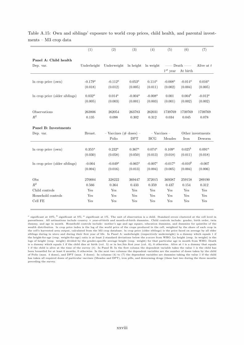
Table A.15: Own and siblings’ exposure to world crop prices, child health, and parental invest-

ments – M3 crop data

(1) (2) (3) (4) (5) (6) (7)

Panel A: Child health

Dep. var. Underheight Underweight ln height ln weight —— Death —— Alive at t

1st year At birth

ln crop price (own) -0.179a -0.112a 0.053a 0.114a -0.008a -0.014a 0.016a

(0.018) (0.012) (0.005) (0.011) (0.002) (0.004) (0.005)

ln crop price (older siblings) 0.032a 0.014a -0.004a -0.008a 0.001 0.004b -0.012a

(0.005) (0.003) (0.001) (0.003) (0.001) (0.002) (0.002)

Observations 263806 262054 263783 262031 1739769 1739769 1739769

R2 0.135 0.098 0.302 0.312 0.034 0.045 0.078

Panel B: Investments

Dep. var. Breast. – Vaccines (# doses) – – Vaccines – Other investments

Polio DPT BCG Measles Iron Deworm

ln crop price (own) 0.355a 0.232a 0.367a 0.074a 0.109a 0.025b 0.091a

(0.030) (0.058) (0.050) (0.013) (0.018) (0.011) (0.018)

ln crop price (older siblings) -0.004 -0.049a -0.065a -0.007c -0.017a -0.010b -0.007

(0.004) (0.016) (0.013) (0.004) (0.005) (0.004) (0.006)

Obs 270004 328222 369447 372015 369387 259158 289190

R2 0.566 0.364 0.433 0.359 0.437 0.154 0.312

Child controls Yes Yes Yes Yes Yes Yes Yes

Household controls Yes Yes Yes Yes Yes Yes Yes

Cell FE Yes Yes Yes Yes Yes Yes Yes

c significant at 10%; b significant at 5%; a significant at 1%. The unit of observation is a child. Standard errors clustered at the cell level in

parentheses. All estimations include country × year-of-birth and month-of-birth dummies. Child controls include: gender, birth order, twin

dummy, and age in month. Household controls include: mother’s age and age square, education dummies, and dummies for quintiles of the

wealth distribution. ln crop price index is the log of the world price of the crops produced in the cell, weighted by the share of each crop in

the cell’s harvested area output, calculated from the M3 crop database. ln crop price (older siblings) is the price faced on average by all elder

siblings during in utero and during their first year of life. In Panel A: underheight (respectively underweight) is a dummy which equals 1 if

the height-for-age (resp. weight-for-age) ratio is at least 2 standard deviations below the z-score from WHO. Ln height (resp. ln weight) is the

logs of height (resp. weight) divided by the gender-specific average height (resp. weight) for that particular age in month from WHO. Death

is a dummy which equals 1 if the child dies at birth (col. 5) or in her/his first year (col. 6), 0 otherwise. Alive at t is a dummy that equals

1 if the child is alive at the time of the survey (t). In Panel B: In the first column the dependent variable takes the value 1 is the child has

been breastfed for at least 6 months, 0 otherwise. In the next two columns the dependent variables are the number of doses taken by the child

of Polio (max. 4 doses), and DPT (max. 3 doses). In columns (4) to (7) the dependent variables are dummies taking the value 1 if the child

has taken all required doses of particular vaccines (Measles and DPT), iron pills, and deworming drugs (these last two during the three months

preceding the survey.

xxviii

C.10 Migration

Given that we look at past income variations, it is possible that the current location of households

is different that their location at the time of the child’s early life. This could induce measurement

error in our agricultural price variable and attenuation bias in our estimates. In this section

we restrict the sample to mothers who have been living in their current location at least since

the child’s birth. This results is a 50% reduction in sample size, mostly because the migration

variable is available for only 60% of the observations. Despite this, our results remain stable.

Table A.16: Exposure to world crop prices, child health and parental investments – Excluding

migrants

(1) (2) (3) (4) (5) (6) (7)

Panel A: Child health

Dep. var. Underheight Underweight ln height ln weight —— Death —— Alive at t

1st year At birth

ln crop price -0.224a -0.157a 0.047a 0.049 -0.016a -0.033a 0.047a

(0.066) (0.044) (0.016) (0.033) (0.005) (0.009) (0.012)

Observations 91414 90117 91414 90117 954504 954504 954504

R2 0.628 0.592 0.755 0.752 0.289 0.289 0.309

Panel B: Investments

Dep. var. Breast. – Vaccines (# doses) – – Vaccines – Other investments

Polio DPT BCG Measles Iron Deworm

ln crop price 0.193a 0.197c 0.326a 0.064b 0.207a 0.017 0.115a

(0.061) (0.113) (0.099) (0.027) (0.039) (0.022) (0.038)

Obs 133167 229689 256275 258791 255523 175762 191610

R2 0.798 0.816 0.824 0.808 0.798 0.817 0.823

Child controls Yes Yes Yes Yes Yes Yes Yes

Mother FE Yes Yes Yes Yes Yes Yes Yes

c significant at 10%; b significant at 5%; a significant at 1%. The unit of observation is a child. Standard errors clustered at the cell level in

parentheses. All estimations include country × year-of-birth and month-of-birth dummies. Child controls include: gender, birth order, twin

dummy, and age in month. ln crop price index is the log of the world price of the crops produced in the cell, weighted by the share of each crop

in the area. In Panel A: underheight (respectively underweight) is a dummy which equals 1 if the height-for-age (resp. weight-for-age) ratio

is at least 2 standard deviations below the z-score from WHO. Ln height (resp. ln weight) is the logs of height (resp. weight) divided by the

gender-specific average height (resp. weight) for that particular age in month from WHO. Death is a dummy which equals 1 if the child dies at

birth (col. 5) or in her/his first year (col. 6), 0 otherwise. Alive at t is a dummy that equals 1 if the child is alive at the time of the survey (t).

In Panel B: In the first column the dependent variable takes the value 1 is the child has been breastfed for at least 6 months, 0 otherwise. In

the next two columns the dependent variables are the number of doses taken by the child of Polio (max. 4 doses), and DPT (max. 3 doses).

In columns (4) to (7) the dependent variables are dummies taking the value 1 if the child has taken all required doses of particular vaccines

(Measles and DPT), iron pills, and deworming drugs (these last two during the three months preceding the survey.

xxix

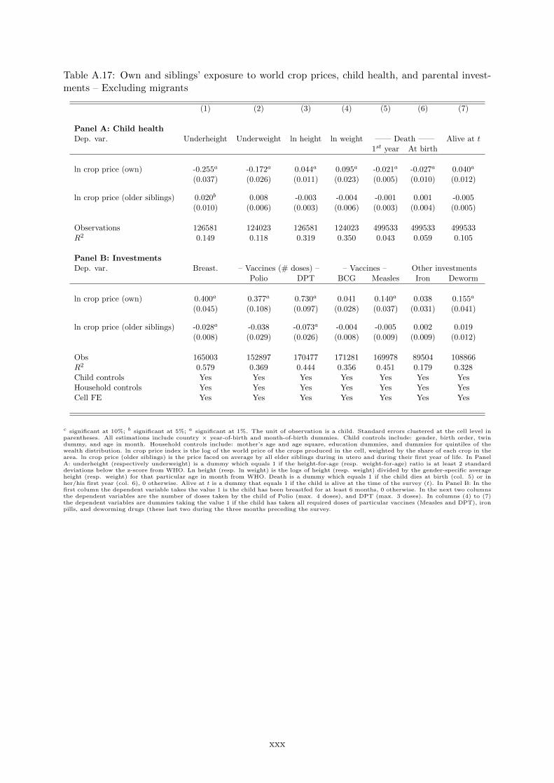
Table A.17: Own and siblings’ exposure to world crop prices, child health, and parental invest-ments – Excluding migrants

(1) (2) (3) (4) (5) (6) (7)

Panel A: Child healthDep. var. Underheight Underweight ln height ln weight —— Death —— Alive at t

1st year At birth

ln crop price (own) -0.255a -0.172a 0.044a 0.095a -0.021a -0.027a 0.040a

(0.037) (0.026) (0.011) (0.023) (0.005) (0.010) (0.012)

ln crop price (older siblings) 0.020b 0.008 -0.003 -0.004 -0.001 0.001 -0.005(0.010) (0.006) (0.003) (0.006) (0.003) (0.004) (0.005)

Observations 126581 124023 126581 124023 499533 499533 499533R2 0.149 0.118 0.319 0.350 0.043 0.059 0.105

Panel B: InvestmentsDep. var. Breast. – Vaccines (# doses) – – Vaccines – Other investments

Polio DPT BCG Measles Iron Deworm

ln crop price (own) 0.400a 0.377a 0.730a 0.041 0.140a 0.038 0.155a

(0.045) (0.108) (0.097) (0.028) (0.037) (0.031) (0.041)

ln crop price (older siblings) -0.028a -0.038 -0.073a -0.004 -0.005 0.002 0.019(0.008) (0.029) (0.026) (0.008) (0.009) (0.009) (0.012)

Obs 165003 152897 170477 171281 169978 89504 108866R2 0.579 0.369 0.444 0.356 0.451 0.179 0.328Child controls Yes Yes Yes Yes Yes Yes YesHousehold controls Yes Yes Yes Yes Yes Yes YesCell FE Yes Yes Yes Yes Yes Yes Yes

c significant at 10%; b significant at 5%; a significant at 1%. The unit of observation is a child. Standard errors clustered at the cell level inparentheses. All estimations include country × year-of-birth and month-of-birth dummies. Child controls include: gender, birth order, twindummy, and age in month. Household controls include: mother’s age and age square, education dummies, and dummies for quintiles of thewealth distribution. ln crop price index is the log of the world price of the crops produced in the cell, weighted by the share of each crop in thearea. ln crop price (older siblings) is the price faced on average by all elder siblings during in utero and during their first year of life. In PanelA: underheight (respectively underweight) is a dummy which equals 1 if the height-for-age (resp. weight-for-age) ratio is at least 2 standarddeviations below the z-score from WHO. Ln height (resp. ln weight) is the logs of height (resp. weight) divided by the gender-specific averageheight (resp. weight) for that particular age in month from WHO. Death is a dummy which equals 1 if the child dies at birth (col. 5) or inher/his first year (col. 6), 0 otherwise. Alive at t is a dummy that equals 1 if the child is alive at the time of the survey (t). In Panel B: In thefirst column the dependent variable takes the value 1 is the child has been breastfed for at least 6 months, 0 otherwise. In the next two columnsthe dependent variables are the number of doses taken by the child of Polio (max. 4 doses), and DPT (max. 3 doses). In columns (4) to (7)the dependent variables are dummies taking the value 1 if the child has taken all required doses of particular vaccines (Measles and DPT), ironpills, and deworming drugs (these last two during the three months preceding the survey.

xxx

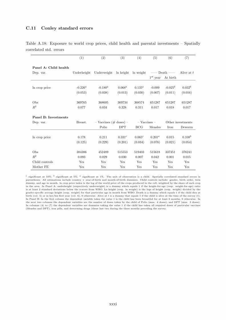
C.11 Conley standard errors

Table A.18: Exposure to world crop prices, child health and parental investments – Spatially

correlated std. errors

(1) (2) (3) (4) (5) (6) (7)

Panel A: Child health

Dep. var. Underheight Underweight ln height ln weight —— Death —— Alive at t

1st year At birth

ln crop price -0.226a -0.180a 0.068a 0.135a -0.009 -0.025b 0.032b

(0.053) (0.038) (0.013) (0.030) (0.007) (0.011) (0.016)

Obs 369765 368605 369734 368574 651287 651287 651287

R2 0.077 0.034 0.328 0.311 0.017 0.018 0.017

Panel B: Investments

Dep. var. Breast. – Vaccines (# doses) – – Vaccines – Other investments

Polio DPT BCG Measles Iron Deworm

ln crop price 0.178 0.211 0.331c 0.065c 0.201a 0.015 0.108b

(0.125) (0.229) (0.201) (0.034) (0.076) (0.021) (0.054)

Obs 384386 452489 515553 519403 515618 337351 376241

R2 0.093 0.029 0.030 0.007 0.042 0.001 0.015

Child controls Yes Yes Yes Yes Yes Yes Yes

Mother FE Yes Yes Yes Yes Yes Yes Yes

c significant at 10%; b significant at 5%; a significant at 1%. The unit of observation is a child. Spatially correlated standard errors in

parentheses. All estimations include country × year-of-birth and month-of-birth dummies. Child controls include: gender, birth order, twin

dummy, and age in month. ln crop price index is the log of the world price of the crops produced in the cell, weighted by the share of each crop

in the area. In Panel A: underheight (respectively underweight) is a dummy which equals 1 if the height-for-age (resp. weight-for-age) ratio

is at least 2 standard deviations below the z-score from WHO. Ln height (resp. ln weight) is the logs of height (resp. weight) divided by the

gender-specific average height (resp. weight) for that particular age in month from WHO. Death is a dummy which equals 1 if the child dies at

birth (col. 5) or in her/his first year (col. 6), 0 otherwise. Alive at t is a dummy that equals 1 if the child is alive at the time of the survey (t).

In Panel B: In the first column the dependent variable takes the value 1 is the child has been breastfed for at least 6 months, 0 otherwise. In

the next two columns the dependent variables are the number of doses taken by the child of Polio (max. 4 doses), and DPT (max. 3 doses).

In columns (4) to (7) the dependent variables are dummies taking the value 1 if the child has taken all required doses of particular vaccines

(Measles and DPT), iron pills, and deworming drugs (these last two during the three months preceding the survey.

xxxi

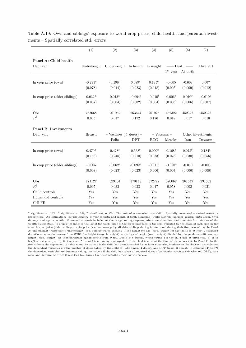
Table A.19: Own and siblings’ exposure to world crop prices, child health, and parental invest-

ments – Spatially correlated std. errors

(1) (2) (3) (4) (5) (6) (7)

Panel A: Child health

Dep. var. Underheight Underweight ln height ln weight —— Death —— Alive at t

1st year At birth

ln crop price (own) -0.295a -0.198a 0.089a 0.195a -0.005 -0.008 0.007

(0.078) (0.044) (0.023) (0.048) (0.005) (0.009) (0.012)

ln crop price (older siblings) 0.032a 0.013a -0.004c -0.010b 0.006c 0.010c -0.019a

(0.007) (0.004) (0.002) (0.004) (0.003) (0.006) (0.007)

Obs 263668 261952 263644 261928 452322 452322 452322

R2 0.035 0.017 0.172 0.176 0.018 0.017 0.016

Panel B: Investments

Dep. var. Breast. – Vaccines (# doses) – – Vaccines – Other investments

Polio DPT BCG Measles Iron Deworm

ln crop price (own) 0.470a 0.428c 0.538b 0.090a 0.168b 0.075b 0.184a

(0.158) (0.248) (0.210) (0.033) (0.076) (0.030) (0.056)

ln crop price (older siblings) -0.005 -0.062a -0.092a -0.011c -0.020a -0.010 -0.003

(0.008) (0.023) (0.023) (0.006) (0.007) (0.006) (0.008)

Obs 271122 329154 370145 372722 370062 261549 291302

R2 0.095 0.032 0.033 0.017 0.058 0.002 0.021

Child controls Yes Yes Yes Yes Yes Yes Yes

Household controls Yes Yes Yes Yes Yes Yes Yes

Cell FE Yes Yes Yes Yes Yes Yes Yes

c significant at 10%; b significant at 5%; a significant at 1%. The unit of observation is a child. Spatially correlated standard errors in

parentheses. All estimations include country × year-of-birth and month-of-birth dummies. Child controls include: gender, birth order, twin

dummy, and age in month. Household controls include: mother’s age and age square, education dummies, and dummies for quintiles of the

wealth distribution. ln crop price index is the log of the world price of the crops produced in the cell, weighted by the share of each crop in the

area. ln crop price (older siblings) is the price faced on average by all elder siblings during in utero and during their first year of life. In Panel

A: underheight (respectively underweight) is a dummy which equals 1 if the height-for-age (resp. weight-for-age) ratio is at least 2 standard

deviations below the z-score from WHO. Ln height (resp. ln weight) is the logs of height (resp. weight) divided by the gender-specific average

height (resp. weight) for that particular age in month from WHO. Death is a dummy which equals 1 if the child dies at birth (col. 5) or in

her/his first year (col. 6), 0 otherwise. Alive at t is a dummy that equals 1 if the child is alive at the time of the survey (t). In Panel B: In the

first column the dependent variable takes the value 1 is the child has been breastfed for at least 6 months, 0 otherwise. In the next two columns

the dependent variables are the number of doses taken by the child of Polio (max. 4 doses), and DPT (max. 3 doses). In columns (4) to (7)

the dependent variables are dummies taking the value 1 if the child has taken all required doses of particular vaccines (Measles and DPT), iron

pills, and deworming drugs (these last two during the three months preceding the survey.

xxxii

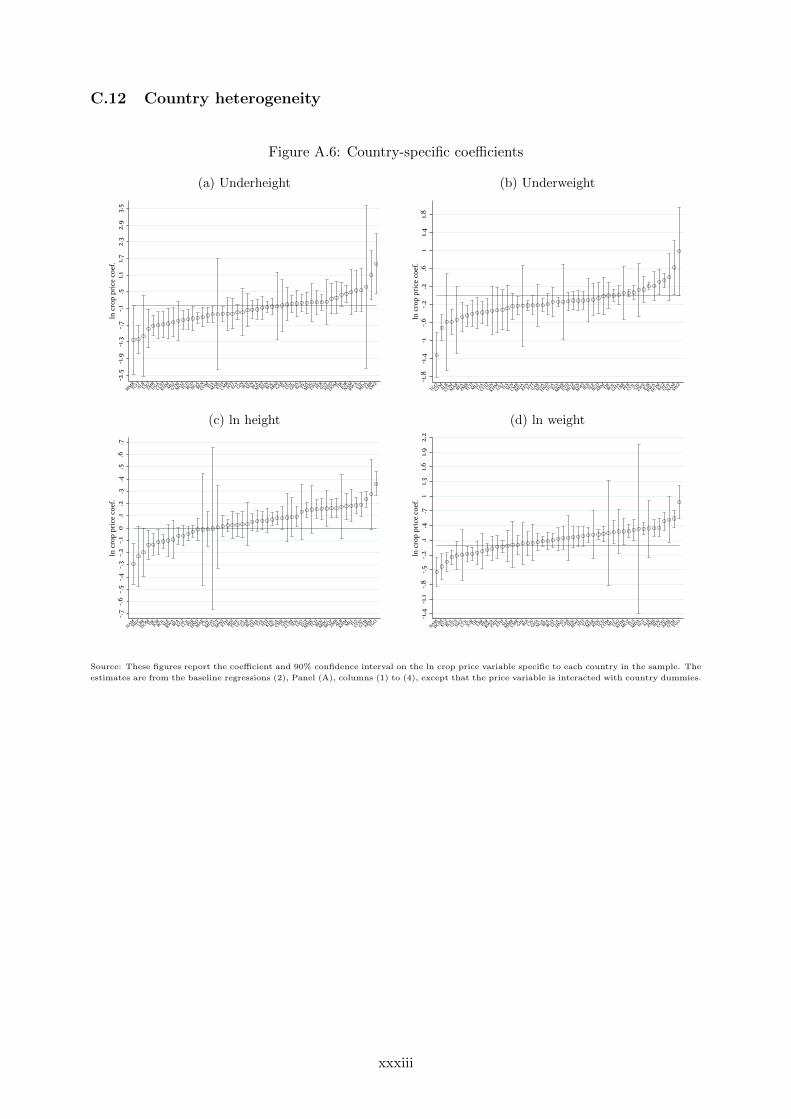
C.12 Country heterogeneity

Figure A.6: Country-specific coefficients

(a) Underheight (b) Underweight

-2.5

-1.9

-1.3

-.7-.1

.51.1

1.72.

32.

93.

5ln

cro

p pr

ice

coef

.

MM

RTGO

ALBLSOZM

BUGA

CODKHMM

LIGTM

MOZ

TCDBGD

NGABEN

COMTLSM

ARETH

CMRHTI

EGYGINBDI

SENBFA

MW

IKEN

BOLARM

GABSL

ECOL

GHAKGZ

TZAM

DGZW

EPER

GUYHND

DOMTJKJORNAM

RWACIV

MDA

LBRSW

Z

-1.8

-1.4

-1-.6

-.2.2

.61

1.41.8

ln c

rop

pric

e co

ef.

TGOGTM

ALBCOM

MAR

BFAZM

BTCD

MLITZA

CODGIN

KHMLSOTLS

SENCM

RM

DAKEN

HTIGAB

NGAHND

UGAEGY

MM

RETH

MOZ

BENM

WIBDI

SLEBGD

ARMTJKBOL

GHALBR

PERCOL

CIVZW

EJO

RRW

ADOM

KGZGUY

NAMSW

Z

(c) ln height (d) ln weight

-.7-.6

-.5-.4

-.3-.2

-.10

.1.2

.3.4

.5.6

.7ln

cro

p pr

ice

coef

.

NAMSW

ZLBR

DOMTJKJORBOL

SLERW

ABFA

KGZCOL

PERHND

MAR

CIVM

DAGUY

MW

IETHBDI

ZWEUGA

GABBGD

GHATZA

HTIKEN

NGACM

RGIN

COMSE

NLSOEGY

MM

RTCD

BENM

DGM

OZZM

BALB

KHMMLI

TLSCOD

GTMARM

TGO

-1.4

-1.1

-.8-.5

-.2.1

.4.7

11.3

1.61.9

2.2

ln c

rop

pric

e co

ef.

NAMDOM

KGZBOL

GUYSW

ZCOL

JORTJKLBR

PERRW

AZW

EETHSL

EM

MRCM

RGINBDI

CIVGHA

NGABFA

BGDUGA

HNDGAB

SENM

WIHTI

TZAM

ARKEN

TCDCOMM

LILSO

KHMM

OZTLS

MDA

EGYALB

ZMBBEN

CODARM

GTMTGO

Source: These figures report the coefficient and 90% confidence interval on the ln crop price variable specific to each country in the sample. The

estimates are from the baseline regressions (2), Panel (A), columns (1) to (4), except that the price variable is interacted with country dummies.

xxxiii

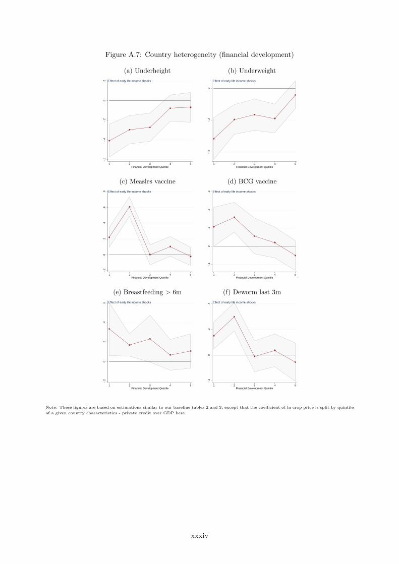
Figure A.7: Country heterogeneity (financial development)

(a) Underheight (b) Underweight

−.6

−.4

−.2

0.2

1 2 3 4 5Financial Development Quintile

Effect of early life income shocks

−.4

−.2

0

1 2 3 4 5Financial Development Quintile

Effect of early life income shocks

(c) Measles vaccine (d) BCG vaccine

−.2

0.2

.4.6

.8

1 2 3 4 5Financial Development Quintile

Effect of early life income shocks

−.1

0.1

.2.3

1 2 3 4 5Financial Development Quintile

Effect of early life income shocks

(e) Breastfeeding > 6m (f) Deworm last 3m

−.2

0.2

.4.6

1 2 3 4 5Financial Development Quintile

Effect of early life income shocks

−.2

0.2

.4

1 2 3 4 5Financial Development Quintile

Effect of early life income shocks

Note: These figures are based on estimations similar to our baseline tables 2 and 3, except that the coefficient of ln crop price is split by quintile

of a given country characteristics - private credit over GDP here.

xxxiv

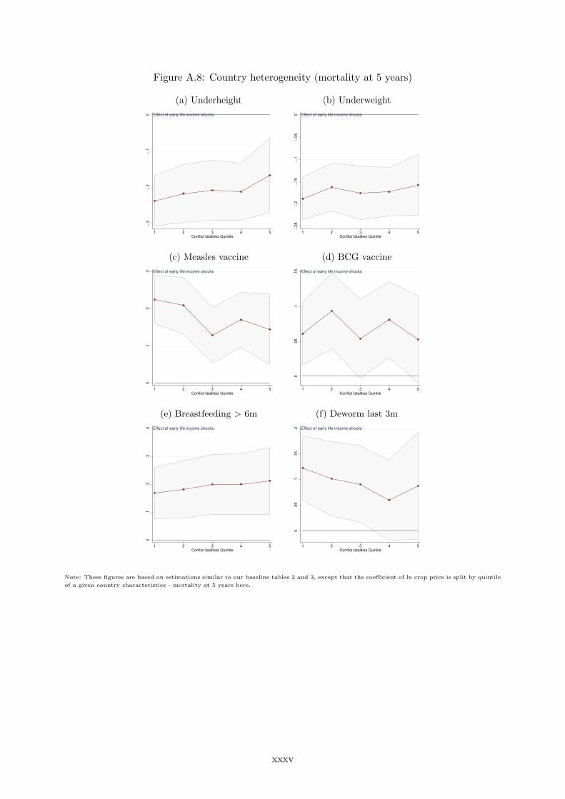
Figure A.8: Country heterogeneity (mortality at 5 years)

(a) Underheight (b) Underweight

−.3

−.2

−.1

0

1 2 3 4 5Conflict fatalities Quintile

Effect of early life income shocks

−.2

5−

.2−

.15

−.1

−.0

50

1 2 3 4 5Conflict fatalities Quintile

Effect of early life income shocks

(c) Measles vaccine (d) BCG vaccine

0.1

.2.3

1 2 3 4 5Conflict fatalities Quintile

Effect of early life income shocks

0.0

5.1

.15

1 2 3 4 5Conflict fatalities Quintile

Effect of early life income shocks

(e) Breastfeeding > 6m (f) Deworm last 3m

0.1

.2.3

.4

1 2 3 4 5Conflict fatalities Quintile

Effect of early life income shocks

0.0

5.1

.15

.2

1 2 3 4 5Conflict fatalities Quintile

Effect of early life income shocks

Note: These figures are based on estimations similar to our baseline tables 2 and 3, except that the coefficient of ln crop price is split by quintile

of a given country characteristics - mortality at 5 years here.

xxxv

Figure A.9: The role of country characteristics

(a) Fractionalization

−.5

−.2

50

.25

.5.7

5

1 2 3 4 5Fractionalization Quintile

Underweight Underheight

Measles vaccine BCG vaccine

Deworm last 3 months Breastfeeding>6m

Effect of early life income shocks on health and investments

Note: This figure is based on estimations similar to our baseline tables 2 and 3, except that the coefficient of ln crop price is split by quintile

of a given country characteristics. Here we use the level of fractionalization, computed as the average of religious, ethnic and linguistic

fractionalization.

Figure A.10: The role of local characteristics

(a) Conflict-related fatalities

−.2

50

.25

1 2 3 4 5Conflict Quintile

Underweight Underheight

Measles vaccine BCG vaccine

Deworm last 3 months Breastfeeding>6m

Effect of early life income shocks on health and investments

Note: This figure is based on estimations similar to our baseline tables 2 and 3, except that the coefficient of ln crop price is split by interval

of a local characteristic. Here we use the cumulated number of fatalities in the cell from UCDP-GED, between 1989 (the first year of conflict

data available) and the year of birth of the child. The first bin contains all cells where no fatality is ever recorded, i.e. more than half for the

cells. The rest of the cells is split in quartiles. Children born before 1990 are dropped from the estimations.

xxxvi

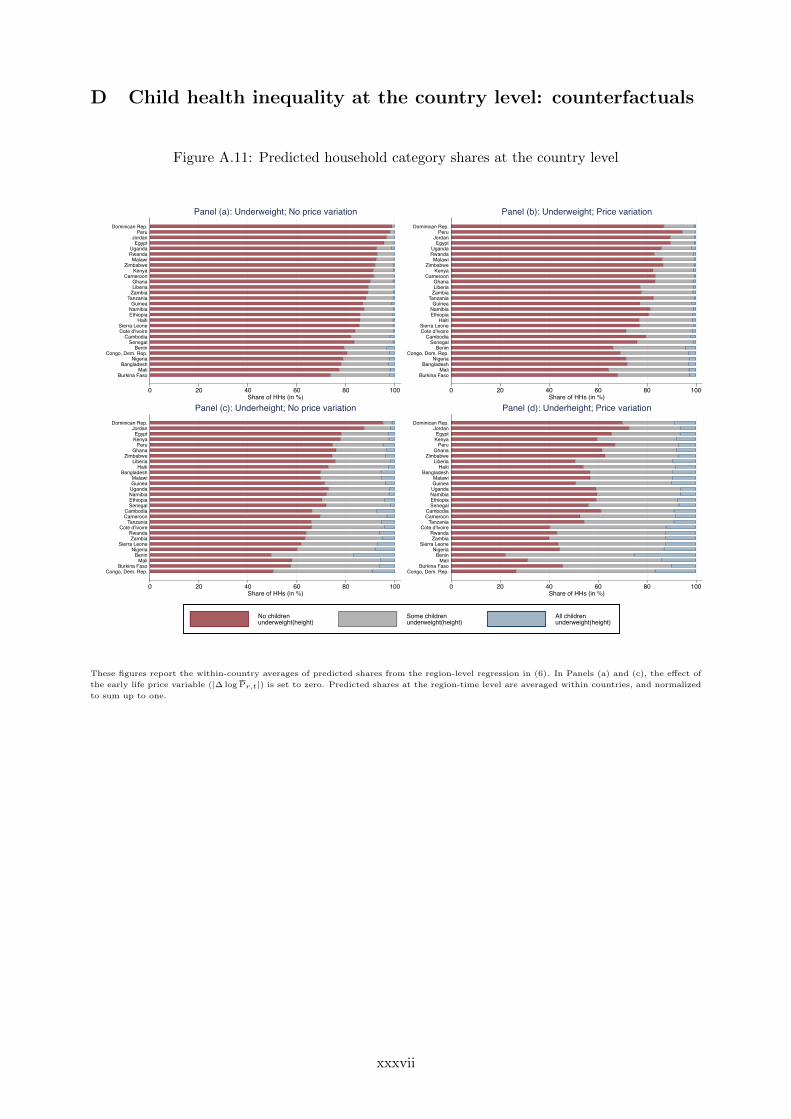
D Child health inequality at the country level: counterfactuals

Figure A.11: Predicted household category shares at the country level

0 20 40 60 80 100Share of HHs (in %)

Burkina FasoMali

BangladeshNigeria

Congo, Dem. Rep.Benin

SenegalCambodia

Cote d'IvoireSierra Leone

HaitiEthiopiaNamibiaGuinea

TanzaniaZambiaLiberiaGhana

CameroonKenya

ZimbabweMalawi

RwandaUganda

EgyptJordan

PeruDominican Rep.

Panel (a): Underweight; No price variation

0 20 40 60 80 100Share of HHs (in %)

Burkina FasoMali

BangladeshNigeria

Congo, Dem. Rep.Benin

SenegalCambodia

Cote d'IvoireSierra Leone

HaitiEthiopiaNamibiaGuinea

TanzaniaZambiaLiberiaGhana

CameroonKenya

ZimbabweMalawi

RwandaUganda

EgyptJordan

PeruDominican Rep.

Panel (b): Underweight; Price variation

0 20 40 60 80 100Share of HHs (in %)

Congo, Dem. Rep.Burkina Faso

MaliBenin

NigeriaSierra Leone

ZambiaRwanda

Cote d'IvoireTanzania

CameroonCambodia

SenegalEthiopiaNamibiaUgandaGuineaMalawi

BangladeshHaiti

LiberiaZimbabwe

GhanaPeru

KenyaEgypt

JordanDominican Rep.

Panel (c): Underheight; No price variation

0 20 40 60 80 100Share of HHs (in %)

Congo, Dem. Rep.Burkina Faso

MaliBenin

NigeriaSierra Leone

ZambiaRwanda

Cote d'IvoireTanzania

CameroonCambodia

SenegalEthiopiaNamibiaUgandaGuineaMalawi

BangladeshHaiti

LiberiaZimbabwe

GhanaPeru

KenyaEgypt

JordanDominican Rep.

Panel (d): Underheight; Price variation

No childrenunderweight(height)

Some childrenunderweight(height)

All childrenunderweight(height)

These figures report the within-country averages of predicted shares from the region-level regression in (6). In Panels (a) and (c), the effect of

the early life price variable (|∆ log Pr,t|) is set to zero. Predicted shares at the region-time level are averaged within countries, and normalized

to sum up to one.

xxxvii