swarm intelligence techniques for task allocation and sub...
TRANSCRIPT

Swarm Intelligence techniques for task
allocation and sub-task merging in
multi-agent systems
Christos Ampatzis
Technical Report No.
TR/IRIDIA/19
03/09/2004
DEA Thesis
Swarm Intelligence techniques for task allocation
and sub-task merging in multi-agent systems
by
Christos Ampatzis——–
Universite Libre de BruxellesFaculte des Sciences Appliquees
IRIDIACP 194/6, Avenue Franklin Roosevelt 50, 1050 Brussels, Belgium
Supervised by
Marco Dorigo, Ph.D.——–
Maıtre de Recherches du FNRSUniversite Libre de Bruxelles
Faculte des Sciences AppliqueesIRIDIA
CP 194/6, Avenue Franklin Roosevelt 50, 1050 Brussels, [email protected]
——–
August, 2004
A thesis submitted in partial fulfillment of the requirements of theUniversite Libre de Bruxelles, Faculte des Sciences Appliquees for the
DIPLOME D’ETUDES APPROFONDIES (DEA)

Abstract
In this work, we address the problem of synthesizing non-reactive controllersfor a swarm robotic system, called swarm-bot, using Artificial Evolution. Inparticular, we evolve simple dynamical neural networks, in order to achieveautonomous decision-making agents that are able to integrate over timetheir perceptual experience. These agents cooperate in carrying out certaintasks by communicating their experience to the rest of the group. We showthe applicability of our desision-making mechanisms in the realisation of acomplex scenario.

Acknowledgments
First of all I would like to thank my supervisor Marco Dorigo for givingme the chance to work on such a challenging project and for his usefulguidance and advice. I would also like to thank especially Vito, but also
Ciro, Rodi, Halva and all people at IRIDIA for providing everydayadvice and help, and for being patient with my initial ignorance. Thanks
also go to Joke for her support, tolerance, patience and love. I wouldalso like to express my admiration for Isaac Asimov, who in his book of1950 “I Robot” (in the story “Runaround”) describes a scene where arobot acts VERY similar to my simulated one. Thanks to Dimitrios
Evangelinos for letting me know. Last but definitely not least, I wouldlike to thank Elio Tuci, for an endless list of reasons: for giving me thechance to work on this very interesting subject, for helping me during thewriting of this document and for priceless advice during my experimental
work. Without Elio I would not have been able to reach this point.

Contents
1 Introduction 1
1.1 Background . . . . . . . . . . . . . . . . . . . . . . . . . . . . 31.1.1 Collective Robotics . . . . . . . . . . . . . . . . . . . . 31.1.2 Metamorphic Robotics . . . . . . . . . . . . . . . . . . 41.1.3 Evolutionary Robotics . . . . . . . . . . . . . . . . . . 5
1.2 Swarm Robotics and The Swarm-Bots Project . . . . . . . . 71.2.1 Swarm Robotics . . . . . . . . . . . . . . . . . . . . . 71.2.2 The SWARM-BOTS project . . . . . . . . . . . . . . 8
1.3 Report Layout . . . . . . . . . . . . . . . . . . . . . . . . . . 11
2 Evolving Time-Dependent Structures 12
2.1 Literature Review . . . . . . . . . . . . . . . . . . . . . . . . 122.2 Integration Over Time . . . . . . . . . . . . . . . . . . . . . . 14
2.2.1 CTRNNs . . . . . . . . . . . . . . . . . . . . . . . . . 172.3 The Tuci et al. Experiment : “Evolving the “feeling” of time
through sensory-motor coordination: a robot based model” . 182.3.1 The simulation . . . . . . . . . . . . . . . . . . . . . . 232.3.2 The controller . . . . . . . . . . . . . . . . . . . . . . . 232.3.3 The evolutionary algorithm . . . . . . . . . . . . . . . 242.3.4 The experiment - The evaluation function . . . . . . . 242.3.5 Results . . . . . . . . . . . . . . . . . . . . . . . . . . 262.3.6 Discussion and Conclusions . . . . . . . . . . . . . . . 28
3 Replicating Tuci et al. in SWARMBOTS3D 31
3.1 Methodological Issues . . . . . . . . . . . . . . . . . . . . . . 313.2 The SWARMBOTS3D Simulator . . . . . . . . . . . . . . . . 32
3.2.1 Sensor, Actuator and Network Configuration . . . . . 343.2.2 The Simulation and the new evaluation function . . . 36
3.3 The Replication with SWARMBOTS3D . . . . . . . . . . . . 37
I

CONTENTS II
3.4 The Minimal Simulation Approach . . . . . . . . . . . . . . . 383.5 Results . . . . . . . . . . . . . . . . . . . . . . . . . . . . . . . 40
3.5.1 The Replication . . . . . . . . . . . . . . . . . . . . . 403.5.2 Analysis of the evolved behavioral strategies . . . . . . 413.5.3 Post Evaluation in the Minimal Simulator Environment 433.5.4 Robustness of the evolved solutions . . . . . . . . . . . 453.5.5 Post Evaluation in SWARMBOTS3D . . . . . . . . . 47
4 Evolving communicating agents 52
4.1 The Task . . . . . . . . . . . . . . . . . . . . . . . . . . . . . 534.2 The Simulation . . . . . . . . . . . . . . . . . . . . . . . . . . 544.3 Results . . . . . . . . . . . . . . . . . . . . . . . . . . . . . . . 57
4.3.1 Post-Evaluation in the Minimal Simulator . . . . . . . 574.3.2 Post-Evaluation in SWARMBOTS3D . . . . . . . . . 60
5 Conclusions 63
5.1 Results . . . . . . . . . . . . . . . . . . . . . . . . . . . . . . . 635.2 Future Work . . . . . . . . . . . . . . . . . . . . . . . . . . . 64

List of Figures
1.1 Graphical visualization of an s-bot. . . . . . . . . . . . . . . . 81.2 Graphical visualization of possible scenarios involving a
swarm-bot. . . . . . . . . . . . . . . . . . . . . . . . . . . . . . 91.3 Picture of the scenario . . . . . . . . . . . . . . . . . . . . . . 10
2.1 The task . . . . . . . . . . . . . . . . . . . . . . . . . . . . . . 202.2 A picture of a Khepera robot on the left. Plan of the robot on
the right, showing sensors and motors. The robot is equippedwith two ambient light sensors (L1 and L2) and a floor sensorindicated by the black square F . The left and right motor (M1
and M2) are controlled by a dynamic neural network (NN).A simple sound signalling system, controlled by an output ofthe network, is referred to as S. . . . . . . . . . . . . . . . . . 22
3.1 The simulated s-bot model . . . . . . . . . . . . . . . . . . . . 333.2 The simulated s-bot models . . . . . . . . . . . . . . . . . . . 343.3 The sound emitting system of the s-bot . . . . . . . . . . . . 363.4 The Fitness during the evolution. The top thin line corre-
sponds to the fitness of the best individual, while the dottedline refers to the average fitness of the population. . . . . . . 38
3.5 Average fitness during the evolution. All plots are the aver-age over the 20 replications of the experiment. The top thinline corresponds to the average fitness of the best individual,while the dotted line below refers to the average fitness of thepopulation. . . . . . . . . . . . . . . . . . . . . . . . . . . . . 41
III

LIST OF FIGURES IV
3.6 Behavioral analysis. The sensor activity and the correspond-ing motor output are plotted for 700 simulation cycles. L1 andL2 refer to the light sensors, while F refers to the floor sensor.M1 and M2 correspond to the motors of the two wheels, andS refers to the sound signalling. When S is bigger than 0.5,the robot emits a signal. . . . . . . . . . . . . . . . . . . . . . 43
3.7 Robustness analysis for run no.20. The offset ∆ is plotted forvarying light-band distance. The box-plot shows 100 evalu-ations per box. Boxes represent the inter-quartile range ofthe data, while the horizontal bars inside the boxes mark themedian values. The whiskers extends to the most extremedata points within 1.5 of the inter-quartile range from thebox. The empty circles mark the outliers. . . . . . . . . . . . 48
4.1 The Fitness during the evolution. The top thin line corre-sponds to the fitness of the best individual, while the dottedline refers to the average fitness of the population. . . . . . . 57

List of Tables
3.1 Post-evaluation. Performance of the ten best evolved con-trollers. The percentage of success (Succ. %) and the per-centage of errors (E1, and E2 in Env.A, and E3, and E4 inEnv.B, ) over 100 trials are shown for both Env.A and Env.B.Additionally, the average offset ∆ and its standard deviation(degrees) are shown for the environment type Env.B. . . . . 46
3.2 Robustness analysis. Performance of the twenty best evolvedcontrollers. The average offset of 100 evolutionary runs isgiven for the mentioned distances between the circular bandand the light. . . . . . . . . . . . . . . . . . . . . . . . . . . 47
3.3 Post-evaluation in SWARMBOTS3D. The percentage of suc-cess (Succ. %) and the percentage of errors (E1, and E2 inEnv.A, and E3, and E4 in Env.B, ) over 100 trials are shownfor both Env.A and Env.B. Additionally, the average offset ∆and its standard deviation (degrees) are shown for the envi-ronment type Env.B. These values are displayed for varioustimesteps and initial robot orientations. . . . . . . . . . . . . 51
4.1 Post-evaluation in the Minimal Simulation environment. Per-formance of the ten best evolved controllers in Env.A. Thepercentage of success (Succ. %) and the percentage of errorsE1 and E2 over 100 trials are shown for both robots. Robot1 is initialised closer to the light source. . . . . . . . . . . . . 60
V

LIST OF TABLES VI
4.2 Post-evaluation in the Minimal Simulation environment. Per-formance of the ten best evolved controllers in Env.B. Thepercentage of success (Succ. %), the reaction time, the per-centage of errors E3, E4 and E5 over 100 trials are shownfor both robots. Additionally, we show the average offset ∆and its standard deviation (degrees) for the first robot thatcompletes the loop. Robot 1 is initialised closer to the lightsource. . . . . . . . . . . . . . . . . . . . . . . . . . . . . . . 61
4.3 Post-evaluation in SWARMBOTS3D. Performance of oneevolved controller in Env.A. The percentage of success (Succ.%) and the percentage of errors E1 and E2 over 100 trialsare shown for both robots. Robot 1 is initialised closer to thelight source. . . . . . . . . . . . . . . . . . . . . . . . . . . . 62
4.4 Post-evaluation in SWARMBOTS3D. Performance of oneevolved controller in Env.B. The percentage of success (Succ.%), the reaction time, the percentage of errors E3, E4 andE5 over 100 trials are shown for both robots. Additionally,we show the average offset ∆ and its standard deviation (de-grees) for the first robot that completes the loop. Robot 1 isinitialised closer to the light source. . . . . . . . . . . . . . . 62

Chapter 1
Introduction
This work addresses the problem of defining the control system for a groupof autonomous robots that have to deal with a non-reactive task. We aimto design neural controllers for a group of autonomous robots equipped withsimple sensors. The robots integrate over time their perceptual experiencesin order to initiate alternative actions. In other words, the behavior of theagents should change as a consequence of their repeated interaction withparticular environmental circumstances. We are interested in exploiting abiologically-inspired evolutionary approach, based on the use of dynamicalneural networks and genetic algorithms [5]. In general, we apply techniquesderived from Artificial Evolution, and we show how they can produce simplebut effective and robust solutions.
There are multiple motivations that lay behind the choice of ArtificialEvolution as a tool for synthesizing controllers for a group of robots. First,Artificial Evolution can bypass many difficulties encountered in the handdesign. In fact, even in a single-robot domain, the problem of designing thecontrol system is not trivial at all and is in fact limited by the designer’s apriori intuitions. The designer must discover the rules that must be encodedinto the controller in order to achieve a certain goal, and decompose the taskinto several subtasks. To do so, it is necessary to know the environment inwhich the robot should act and to predict the outcome of a sequence ofactions performed by the robot. When the environment is dynamic andunpredictable, designing the control system could be very challenging. In adistributed multi-robot domain, this problem is worsened by the fact thateach robot is an independent entity that can take its own decisions de-pending on the current sensory input information, but also on its internalstate. Furthermore, robots interact with each other, making the system
1

CHAPTER 1. INTRODUCTION 2
much more dynamic and complex. The designer must be capable of pre-dicting the outcome of such interactions, which could be extremely difficult,even impossible. On the contrary, Artificial Evolution does not suffer fromthis problem since it is an automatic process that directly tests the behaviordisplayed by the robots embedded in their environment and selects out thebad-performing individuals. This approach, working in a bottom-up direc-tion, bypasses the decomposition problems given by a top-down approach,typical of behavior-based or rule-based systems, being relatively unbiased.Furthermore, Artificial Evolution can exploit the richness of solutions offeredby the complex dynamics resulting from robot-robot and robot-environmentinteractions.
In this work, we present the results obtained from the ongoing workwithin the SWARM-BOTS project1. The aim of the SWARM-BOTS projectis the development of a new robotic system, called a swarm-bot [55, 40]. Theswarm-bot is defined as an artifact composed of simple autonomous robots,called s-bots. An s-bot has limited acting, sensing and computational ca-pabilities, but can create physical connections with other s-bots, thereforeforming a swarm-bot that is able to solve problems the single individualcannot cope with. Up to now, in the project have been studied only reactivebehaviors. We chose to study integration over time, a non-reactive task,that is a task that in order to be carried out by the robot, needs “mem-ory”. The robot’s behavior will not only be affected by its current sensorystatus, but also by its internal dynamics. At this specific moment in theproject, the study of efficient decision-making mechanisms is necessary inorder to succeed in integrating different behaviors exhibited by the swarm-bot, for which efficient controllers have already been successfully evolved.The work described in this paper will tackle the problem of designing acontroller which is able to integrate sensorial information over time and ad-just its subsequent behavior accordingly. With the use of communication,we will expand its functionality for a group of robots. For more details onthe significance of this work for the project, the reader is suggested to seeSection 1.2.2. In the rest of this chapter, we first present the state-of-the-art, describing the research fields that constitute the starting point of thiswork (see Section 1.1). In Section 1.2, after some general information andstate-of-the-art, we present in detail the SWARM-BOTS project and ourcontribution to it. Finally, Section 1.3 briefly summarizes the contents ofthis thesis.
1A project funded by the Future and Emerging Technologies Programme (IST-FET)of the European Community, under grant IST-2000-31010.

CHAPTER 1. INTRODUCTION 3
1.1 Background
In the last decade there has been a growing interest in the development ofcomplex robotic systems which could present features like versatility, ro-bustness or capacity to perform complex tasks in unknown environments.In order to achieve these features, the single-robot approach was often aban-doned in favor of more complex systems, involving multiple robots workingin strict cooperation. In fact, developing and controlling a single, multi-purpose robot is a complex task, that can also prove to be very expensive.Another problem that might be experienced with the single-robot approachis that even small failures may prevent the accomplishment of the whole task.A group of simple and cheap robots may be able to efficiently accomplishmany tasks that go beyond the capabilities of the individual robot. Thisidea is the cornerstone of the research in the Collective Robotics field andin the Metamorphic Robotics field, which cover most of the related researchdone so far. On a parallel track, the research in autonomous robotics hasfaced the challenge of synthesizing the controllers for such robotics systems.Among the different approaches that have been proposed, we are mainlyinterested in the study of Evolutionary Robotics, which applies techniquesderived from Artificial Evolution to the development of controllers for au-tonomous robots (for a review see [45]). In this section, we present thestate-of-the-art in all these research fields, which constitutes the startingpoint of our research.
1.1.1 Collective Robotics
The field of Collective Robotics focuses on the study of robotic systemsthat are composed of a number of autonomous robots which act togetherin order to reach a common goal (for an overview of the field, see [49]).The main motivation behind the study of collective robotic systems lays inthe possibility to decompose the solution of a complex problem into sub-problems that are simpler and that can be faced by simple robotic units.
Collective robotics research has mainly focused on the achievement ofcoordination of several systems. For example, Gerkey and Mataric [23] pro-pose a dynamic task allocation method based on auction exchange in orderto achieve cooperation in a group of robots. Agassounon et al. [2] use ascalable algorithm based on a threshold model for the allocation of robotsin a puck collecting and clustering task. Melhuish [38] describes a clusteringtask collectively performed by a group of cooperating robots. Schenker etal. [56] summarize the robotics work being carried out at NASA Jet Propul-

CHAPTER 1. INTRODUCTION 4
sion Laboratory. They report on the development of RWC (a multi-RobotWork Crew), which consists of cooperating rovers controlled a decentralisedbehavior-based control architecture. It is an interesting approach since itis designed not only for cooperative group behaviors but also for tightlycoordinated tasks such as the transporting of large payloads [51].
Another interesting aspect of collective robotics is given by the robust-ness that can be achieved by providing redundancy to the whole system.For example, Parker [48] defined a software architecture for fault tolerantcontrol of heterogeneous robots which allows a robot to select the correctaction to be performed depending on the requirement of the mission, theactivities of the other robots, the environmental conditions, and its own in-ternal state. Goldberg and Mataric [24] demonstrate the effectiveness of abehavior-based approach for the definition of robust and easily modifiablecontrollers for distributed multi-robot collection tasks.
A controversial aspect in the collective robots community is given bythe use of communication. In some cases, communication can be useful formodelling the internal state of other agents, or for communicating the exe-cution of a particular action to a teammate, as will also be the case in ourwork. Bonarini and Trianni [9] have shown that the communication of “co-operation proposals” can help learning cooperative behaviors. Mataric [37]showed how communication can be used to transmit sensory information toother robots in order to increase the coordination of the group. Communi-cation was also used as a mean to distribute reward to other members of thegroup in a reinforcement learning task. Balk and Arkin [3] have shown thatcooperation can emerge in a group of robots if they are not able to inde-pendently accomplish a given task. They show that, depending on the task,communication may or may not be helpful, and that often very simple formsof communication are sufficient to the accomplishment of a cooperative task.
1.1.2 Metamorphic Robotics
The major effort in Metamorphic Robotics research has been to study singlerobots composed of a collection of identical modules where each module isa simpler robot. Usually, every module is in contact with at least anothermodule so that a more complex structure is defined. All modules have thesame physical structure and each module is autonomous from the viewpointof computation and communication.
Chirikjian et al. [14] describe a metamorphic robot composed of iden-tical hexagonal modules that can aggregate as a two-dimensional structurewith varying geometry. Robot configuration is computed by a centralized

CHAPTER 1. INTRODUCTION 5
control that uses mathematical properties of the lattice connectivity graphassociated to the structure. The work is closer to geometrical and kinemat-ics research where the goal is to compute the minimum number of moves toreach a given configuration rather than to the problem of controlling in realtime a complex robot structure. Yim et al. [69] have developed PolyBot, ametamorphic robot defined by a sophisticated basic module with on-boardcomputing capabilities. Also in this case, however, the robot shape is de-fined by a centralized control. Murata et al. [41] consider a system of 2Dmodules called Fracta that can achieve planar motion by walking over eachother. The reconfiguration motion is actuated by varying the polarity of elec-tromagnets that are embedded in each module. Kamimura et al. [34] havedeveloped MTRAN, which got a lot of attention due to excellent results withreal hardware. This system uses a large number of modules with only onedegree of freedom and can self-reconfigure. Shen et al. [57, 13] with CONROproposed another work that follows the above-mentioned directions. Robotmorphology is ensured by modular identical structures strongly coupled byphysical connectors. Robot shapes are predefined and module moves are pre-computed by planners based on global information while no effort is madeon distributed/on-line control, adaptation and self-reconfiguration. Only re-cently, a decentralized control has been developed for this system by Støyet al. [58]. This system allows to manually change the position of the hard-ware modules in the structure while the system is running and each moduleautonomously re-adapts its behavioral role in the system.
1.1.3 Evolutionary Robotics
The problem of defining a controller for a robotic system has been ap-proached from many different directions: inferential planners, behavior-based robotics and learning classifier systems are only some examples of thepossible ways of controlling a robot. Among these, Evolutionary Roboticsis a very promising technique for the synthesis of robot controllers [45]. Itis inspired by the Darwinian principle of selective reproduction of the fittestindividual in a population. The process of searching the design space bymimicking natural evolution is generally referred to as Evolutionary Algo-rithms. In this thesis we will employ a particular type of EvolutionaryAlgorithms called genetic algorithms [31]. A genetic algorithm works asfollows: starting from a population of genotypes, each encoding the con-trol system (and sometimes the morphology) of the robot, the evolutionaryprocess evaluates the performance of each individual controller, letting therobot free to act in its environment following the genetically encoded rules.

CHAPTER 1. INTRODUCTION 6
The fittest robots are allowed to reproduce, generating copies of their geneticmaterial, which can be changed by several genetic operators (e.g., mutation,crossover). This process is iterated a number of times (generations) untila satisfying controller is found that meets the requirements stated by theexperimenter in the performance evaluation (fitness function).
Evolutionary Robotics provides us with a unique opportunity to cou-ple an agent’s dynamical system with the environment’s dynamical system,through sensory-motor interactions. By exhibiting both situatedness andembodiment, it evaluates a solution based on the agent’s interaction withits enviroment [30].
Many difficult control problems have been easily solved relying on theevolutionary approach. For example, Nolfi [42] successfully evolved a con-troller for the Khepera robot [39] in order to find and stay close to a targetobject. The Khepera, equipped only with infrared proximity sensors, wasplaced in a rectangular arena surrounded by walls and containing the tar-get cylindrical object that had to be found. The evolved controller didvery well, while this task is very difficult to be solved by hand design—with a behavior-based controller. In fact, a difficult discrimination mustbe performed between the sensory pattern generated by a wall and the onegenerated by the target obstacle. Harvey et al. [29] addressed the problemof navigation acquiring information about the evironment from a camera.They evolved both the morphology of the visual receptive field and the ar-chitecture of the neural network. Using these settings, they successfullysynthesized an individual for approaching a triangular shape painted on awall and at the same time avoiding a rectangular one, guided by the visionsystem. Floreano and Mondada [19] evolved a homing navigation behaviorfor a Khepera robot, using a recurrent neural network. They showed thatthe internal dynamics of the recurrent network could encode a sort of mapof the environment that leads to an efficient homing behavior.
More recently, the evolutionary robotic community has approached theproblem of defining collective behaviors. For example, Baldassare et al. [4]evolved group behaviors for simulated Khepera robots, which had to aggre-gate and navigate toward a light target. Quinn [52] evolved coordinatedmotion behaviors with two Khepera. On the same track, Quinn et al. [53]studied coordinated motion with three wheelchair robots.

CHAPTER 1. INTRODUCTION 7
1.2 Swarm Robotics and The Swarm-Bots Project
1.2.1 Swarm Robotics
Swarm robotics is a novel approach to the design and implementation ofrobotic systems. These systems are composed of swarms of robots whichtightly interact and cooperate to reach their goal. Swarm robotics can beconsidered as an instance of the more general field of collective robotics (seeSection 1.1.1). It is inspired by the social insect metaphor and emphasizesaspects like decentralization of the control, limited communication abilitiesamong robots, emergence of global behavior and robustness. In a swarmrobotic system, although each single robot composing the swarm is a fullyautonomous robot, the swarm as a whole can solve problems that the singlerobot cannot solve because of physical constraints or limited abilities.
Sugawara et al. have studied different aspects of swarm robotic systems.In [59], they study the task of gathering pucks to a fixed point under differentdistributions of pucks in the environment. When a robot found a puck,it stopped and emitted light for a certain time duration, to broadcast itsposition. The emitted light served as an attraction field to other unladenrobots. The performance of the swarm was measured through the percentageof collected pucks with respect to time. Among other things, the authorshave also presented results for the aggregation of the robots, resembling thatof amoebae. The authors also proposed an analytical model of the swarmrobotic system, to explain some of the dynamics of the system.
Payton et al. [50] work on the Pheromone Robotics project and havebuilt a swarm robotic system in order to study the coordination of robotsfor tasks such as surveillance, reconnaissance, hazard detection and pathfinding. The system consisted of a group of mobile robots, called pher-obots, that can locally communicate with each other using infrared-basedtransceivers mounted on them.
DARPA (Defense Advanced Research Projects Agency) awarded a grantto Icosystem Corporation (http://www.icosystem.com) to apply swarm in-telligence methods to the control of robotic swarms. The project is titled“Design of Control Strategies for Swarms of Unmanned Ground Vehicles”and it proposes to develop strategies to control swarms of robots carryingout indoor navigation and reconnaissance tasks. The underlying researchgoal of this project is to address a number of fundamental questions aboutswarm control [66, 22].
Bruemmer et al. [12] report on the use of social potential attractiveand repulsive fields emitted by each robot, as a means to coordinate group

CHAPTER 1. INTRODUCTION 8
behavior and promote the emergence of swarm intelligence. They tackle theproblem of spill finding and perimeter detection by a swarm of robots.
Gaudiano et al. [21] studied the control of a swarm of UAVs (UnmannedAir Vehicles). The work is done in simulation for the problems of search overa region (which can also be seen as an area coverage task). They simulateddifferent strategies and analyzed their efficiencies.
1.2.2 The SWARM-BOTS project
As mentioned above, this work is carried out within the SWARM-BOTSproject, whose aim is the development of a swarm robotic system, calledswarm-bot. A swarm-bot is defined as an artifact composed of a swarm ofs-bots, mobile robots with the ability to connect to/disconnect from eachother. S-bots have simple sensors and motors and limited computationalcapabilities. Their physical links are used to assemble into a swarm-bot ableto solve problems that cannot be solved by a single s-bot (see Figure 1.1).
Figure 1.1: Graphical visualization of an s-bot.
The swarm-bot concept lies between the two main streams of roboticsresearch described above, that is, collective robotics and metamorphicrobotics. In fact, in collective robotics, autonomous mobile robots inter-act with each other to accomplish a particular task, but, unlike s-bots, theydo not have the ability to attach to each other by making physical connec-tions. On the other hand, a self-reconfigurable robotic system consists ofconnected self-contained modules that, although autonomous in their move-ment, remain attached to each other, lacking the full mobility of s-bots.
In the swarm-bot formation, the s-bots are attached to each other andthe robotic system is a single whole that can move and reconfigure alongthe way when needed. For example, it might have to adopt different shapesin order to go through a narrow passage or overcome an obstacle. Physical

CHAPTER 1. INTRODUCTION 9
connections between s-bots are important for building pulling chains, as forexample in an object retrieval scenario (see Figure 1.2a). They can alsoserve as support if the swarm-bot is going over a hole larger than a single s-bot, as exemplified in Figure 1.2b, or when the swarm-bot is passing througha steep concave region, in a navigation on rough terrain scenario. Anyway,there might be occasions in which a swarm of independent s-bots is moreefficient: for example, when searching for a goal location or when trackingan optimal path to a goal.
(a) (b)
Figure 1.2: Graphical visualization of possible scenarios involving a swarm-bot. (a) Retrieving a circular object. (b) Passing over a trough.
The above examples represent the family of tasks a swarm-bot should beable to perform. Although these tasks present many differences from eachother, they share many common aspects, among which the capability toperform aggregation and to distributely coordinate the activity of the group.Aggregation is definitely of utmost interest because it is a prerequisite forthe development of other forms of cooperation: for example, in order toassemble in a swarm-bot, s-bots should first be able to aggregate. On theother hand, the ability to coordinate the activities of the group is crucialfor the effectiveness of a swarm-bot : for example, when carrying a heavyobject that a single s-bot cannot move, all s-bots should coordinate and pullor push in the same direction, in order to maximize the performance of theswarm-bot.
Up to now, the project’s empirical work has focused on the study ofCoordinated Motion (see [16]), Cooperative Transport (see [26, 27]), ChainFormation and Task Allocation(see [36, 35]). The final goal of the project isthe successful realization of a scenario described in detail in [15]. Figure 1.3gives an approximate idea about the settings of this scenario.
A swarm of up to 35 s-bots must transport a heavy object from its initial

CHAPTER 1. INTRODUCTION 10
Figure 1.3: Picture of the scenario
location to a goal location. There are several possible paths from the initialto the goal location and these paths may have different lengths and mayrequire avoiding obstacles and holes. The weight of the object is such thatits transportation requires the coordinated work of at least n s-bots, wheren is a parameter . Since the “building blocks” of the overall behavior exist,we need a strategy that will provide us with an effective decision makingmechanism, for swapping between strategies. We also need a strategy thatwill allow each s-bot to realise its current status in the work it is carryingout. For example, robots that explore the enviroment in order to find thegoal location, might encounter holes in it, as shown in the above picture.They need to be able to make a decision as to if the hole can be traversed bya single robot. If this is not the case, to call for help, resulting in a swarm-botformation which might be more effective in passing over this gap. Definitely,it is a “cheaper” solution if one robot can solve the task alone, but we areinterested in cases where this is not possible. Thus, the work demonstratedin this thesis addresses the problem of evolving neural network controllerswhich will be able to produce this decision-making mechanism, which inturn will contribute to the realization of the scenario. Our goal is to solvea simplified part of it, which will be the first step in the realization of thecomplete complex scenario, capturing the elements of a decision-makingmechanism. More in detail, our work is focused on the design of controllersevolved to tackle non-reactive problems, problems where a simple reactivebehavior is not enough to solve the task, but a kind of “memory” and internaldynamics are necessary. Consequently, we will result in controllers consistingin a very different structure compared to what has been used up to now inthe project.

CHAPTER 1. INTRODUCTION 11
1.3 Report Layout
This report is organized as follows. In Chapter 2 we discuss about the moti-vation that led us to the choice of integration over time as a decision makingmechanism for the swarm-bot. We present the work of Tuci et al. [65] whichis the starting point of this research and discuss its limitations, discussingpossible extentions and adaptations in order for this idea to fit into theSWARM-BOTS project context.
In Chapter 3, we present the setup used for a first set of experimentsperformed, the replication of the work of Tuci et al. in a physics-based 3Denviroment. We provide the motivation for the experiments performed andfor the simulation model used, by introducing the notion of Minimal Simu-lation, as defined by Jakobi in [32]. We will show that since our experimentsdon’t require dynamics and physics, they can be conducted within a MinimalSimulation environment. The latter is much faster than a 3D physics-basedsimulator. We also describe the simulation, controller and evolutionary al-gorithm we employed in all the performed experiments. Finally, we providethe results obtained and an analysis performed.
In Chapter 4, we present a second set of experiments performed, ex-tending the work presented in 3, the results obtained and their statisticalanalysis. This time, the task is more oriented towards a Collective Roboticsscenario, since it requires communication between two robots.
In Chapter 5, we draw the conclusions of this work, highlighting theimportant aspects of this research. Finally, we indicate the possible futureresearch directions to be followed.

Chapter 2
Evolving Time-Dependent
Structures
Several studies have described evolutionary simulation models in which time-dependent structures are evolved to control the behavior of agents requiredto make decisions based on their experiences. The aim of Section 2.1 is topresent the related work in literature, introducing the distinction betweenecological and non-ecological models. Section 2.2 gives an overview of theworks introducing integration over time while in Section 2.3 we present indetail the Tuci et al. experiments, which are the starting point and inspira-tion of the work presented in this thesis.
2.1 Literature Review
It is useful to draw a line between two lines of research present in the liter-ature, in a very simple way. These are non-ecological and ecological mod-els [60, 61, 68, 63]. In ecological models, like the one by Tuci et al. [65],described in detail in the following section, and our experimental work, theagent’s perception is brought forth by the agent itself through its actions.Contrary to that, in the non-ecological models the perceptual experience ofthe agents is determined by the experimenter. Obviously, the flow of percep-tion provides the agents the cues to make the discrimination (for more onthis issue see also [47]). The input to the network is not determined by thenetwork’s output at previous timestep. That is, the network does not bringforth the world which it experiences through its sensors. Moreover, some ofthe non-ecological models (see [68]) are further simplified by the presenceof an explicit reinforcement signal—i.e., an input signal explicitly dedicated
12

CHAPTER 2. EVOLVING TIME-DEPENDENT STRUCTURES 13
to inform the agent’s controller on the characteristics of the “environmentalcircumstances” in which it is currently situated by making available to thesystem any possible mismatch between the current agent’s action and thecorrect response.
For example, in [63], populations of CTRNNs (Continuous-Time Recur-rent Neural Networks) are evolved to solve the “Dowry Problem”—a sequen-tial decision problem in which an agent has to maximise the expected payoffgiven by choosing a single item from among a population of sequentially en-countered items. The latter appears to the agent in random order, and theyare drawn from a population with parameters that are completely unknownahead of time. The sequence of items presented to the network is not in anycase affected by the response of the agent at previous time. The results of thesimulations show that evolved CTRNNs are capable of sampling a certainproportion of the population of items that is currently experiencing to getan estimation of the distribution of values, and subsequently to exploit thisinformation and make a choice. In [68], an “abstract” agent—i.e., a disem-bodied dynamic neural network—was responsible of solving the integrationof reactive and non-reactive behaviors consisting mainly in generating theappropriate n-bit sequence chosen from either two, three, or four possibledifferent sequences.
Other studies on the evolution of time-dependent structures for discrimi-nation tasks share with ours and the Tuci et al. experiment a more ecologicalperspective, in which the nature of the agent’s perception is determined byits own actions, and the reinforcement signals are part of the evolved struc-tures (see [70, 64, 44, 8]). The evolution of time-dependent structures anddecision-making mechanisms has been extensively studied on the T-mazeproblem (see [70, 8]). The robot is required to find its way to a goal loca-tion, placed at the bottom of any of the two arms of the maze. When at theT junction, the robot must decide whether to turn left or right. The correctdecision can be made if the agent is capable of exploiting perceptual cueswhich were available to it while it was navigating down the first corridor,or by “remembering” something about previous trials in a similar T-maze.In [70], weight change mechanisms provide the agents the required plastic-ity to exploit the relationship between the location of light signals placedroughly at the middle of the first corridor, and the turn to make at thejunction. Blynel et al. in [8] allow the agent to experience the environmentin a first trial, in which the success or failure play the role of a reinforce-ment signal, in order to associate the position of the goal with respect tothe T-junction.
In [64], evolved CTRNNs provide the agents the required plasticity to

CHAPTER 2. EVOLVING TIME-DEPENDENT STRUCTURES 14
discover the spatial relationship between the position of a landmark andthe position of a goal. In this study, the spatial relationship between thegoal and the landmark can be learnt by “remembering” from previous trialsthe relative position of the landmark with respect to the goal. The workillustrated by Nolfi in [44] investigates a discrimination task in which a robot,while navigating through a maze, must recognise if it is located in one roomrather than another. Here, the agent exploits environmental cues, such asnavigating through subsequent corners of the maze, and fine-tuned time-dependent structures to take the correct decision. Environmental structures(regularities) are at the basis of the recognition process performed by theagent’s controller during the exploration of the maze.
The difference between the ecological models and our study is not asapparent as it was for the non-ecological ones described at the beginningof the section. However, it should be noticed that, in the ecological studiesreviewed above, the discrimination is based on the recognition of distinc-tive environmental contingencies and the maintenance of these experiencesthrough time, as a form of short term memory. On the contrary, in ourstudy, the cue which allows the agent to make the discrimination has todeal with the persistence over time of a perceptual state common to bothof the elements to be distinguished—i.e., Env.A and Env.B—rather thanwith the nature of the cue itself employed to make the discrimination. Thatis, in our case, due to the nature of the agent’s sensory apparatus, the twotypes of environment can be distinguished solely because a perceptual state,present in both environments, might be perceived by the agent for a longertime in one than in the other.
2.2 Integration Over Time
A general problem common to biology and robotics concerns the definitionof the mechanisms necessary to decide when it is better to pursue a partic-ular action in a certain location and at which moment in time it is betterto leave for pursuing a similar or a different activity in a similar or differentlocation. This problem is not limited to foraging alone, but it extends tomany activities a natural or artificial agent is required to carry out. Au-tonomous agents may be asked to change their behavior in response to theinformation gained through repeated interactions with their environment.For example, in a group of robots, although many individual actions mightbe simpler to carry out than a single coordinated activity, they might re-sult less efficient (see [62]). Therefore, autonomous agents require adaptive

CHAPTER 2. EVOLVING TIME-DEPENDENT STRUCTURES 15
mechanisms to decide whether it is better to pursue solitary actions or toinitiate cooperative strategies. Also, an agent might need to communicateto the other members of the group some information it has gathered. Thescenario described in Section 1.2 requires such a behavior. For example, therobots should find a way to the goal area, and to do so they have to exploretheir enviroment, which might contain holes or areas dangerous to traverse.We need a strategy which will allow such agents to decide if alternativestrategies are required and thus trigger cooperation through communicationof their experience.
One way to deal with the challenge described above is the design ofdecision-making mechanisms for —in our case— an s-bot, which integratesover time its perceptual experience in order to initiate alternative actions.In other words, the behavior of the agent should change as a consequenceof its repeated interaction with particular environmental circumstances.
Nolfi et al. define agents that exploit internal representations as well asinformation directly available from their sensors and that are able to extracttheir internal representations autonomously by interacting with the environ-ment, as agents that are able to integrate sensory-motor information overtime. They rely on a mixed strategy in which basic sensory-motor mecha-nisms are complemented and enhanced with additional internal mechanismsand tend to rely on partial, action-oriented, and action-mediated represen-tations of the external environment [46].
In this thesis we call upon the notion of internal representation, a verycontroversial issue in the literature. It can be more properly characterizedas a description that is in the eye of the observer rather than as a formalproperty of an agent. We do not want to get into details in this subject,therefore we will resort on the more general notion of internal state. Byinternal state we mean a state (e.g. the activation state of an internalneuron of the control system of a robot) that might be affected by the pre-vious sensory-motor states experienced by the robot and that co-determine,together with the current sensory states, the robot’s motor actions. By me-diating between perception and actions, internal states might allow agentsto produce behaviors that are decoupled from the immediate circumstanceswhile still remaining sensitive to them. We will use the definition introducedby Nolfi et al. in [46]. Thus, a reactive robot is a robot that does not haveany internal state and for which the current motor action is only dependentof the current sensory state. On the contrary, a robot that relies exclusivelyon its internal dynamics is a robot in which sensory information comingfrom the external environment is either missing or not taken into accountonce the robot motor actions are determined. A very important observation

CHAPTER 2. EVOLVING TIME-DEPENDENT STRUCTURES 16
to be made is that a robot with a non-reactive controller can also exhibitreactive behavior.
Most of the experiments in evolutionary robotics rely on neural con-trollers. In many cases feed-forward neural networks are used. These net-works are effective in producing reactive behavior but cannot deal with time,always reacting in the same way to the same sensory state and therefore can-not integrate information over time. In other cases recurrent neural networkshave been used (see [18]). Other attempts have been conducted by usingContinuous Time Recurrent Neural Networks (CTRNNs) [7]. By relyingon differential equations instead of being updated at fixed time steps thesenetworks can produce continuous dynamics. These networks have been suc-cessfully applied to a variety of tasks (such as legged locomotion [33] andvisually guided navigation [29]). However the extent to which they can beapplied to tasks that have sequential components and their ability to scale upis unclear. Other attempts have been conducted by using synaptic plastic-ity. In some cases the synaptic weights were updated by using reinforcementlearning (see [1]) or back-propagation (see [54]) on the basis of self-generatedteaching signals. In other cases synaptic weights were updated on the basisof genetically encoded hebbian rules (see [20]). In general terms, integrationof information over time can be accomplished both by modifying the synap-tic weights (through some form of plasticity) and by means of recurrentconnections. In both cases in fact, the way in which individuals react to thecurrent sensory state might be affected by the previous experienced sensorystates. Different methods however might have different characteristics. Forinstance, the former approaches, by relying on gradient descent techniques,tend to produce small and long term effects on the robot behaviors whereasthe latter approach, based on hebbian learning, might produce significanteffects in the short term [20].
So, we can expect the emergence of systems able to integrate sensory-motor information over time and later use this information to modulate theirbehavior accordingly under certain conditions. First of all, as we discussedabove, the agent should be equipped with the appropriate neural controller,able to display non-reactive behavior. But then, how do we distinguishbetween the tasks that require integration over time and those that don’t?The border between what can be accomplished by simple agents that onlyrely on their current sensory states or on their internal dynamics and whatcan be accomplished by more complex agents that are also able to integrateinformation over time is rather fuzzy and cannot be formally identified.However, problems that should be accomplished in varying environmentalconditions tend to require agents able to integrate information over time [46].

CHAPTER 2. EVOLVING TIME-DEPENDENT STRUCTURES 17
2.2.1 CTRNNs
Continuous Time Recurrent Neural Networks (CTRNNs) have been intro-duced in Evolutionary Robotics by Beer [6], and they are the reflection ofa theoretical approach to cognition which aims to exploit the mathematicaltools of dynamical systems theory to investigate issues of interest in adaptivebehavior research. According to Beer, there are two fundamental principleswhich justify the use of the formalism of dynamical systems theory withinthe context of adaptive behavior. Firstly, since the fundamental nature ofadaptive behavior in natural systems is to generate the appropriate behav-ior at the appropriate time, dynamical systems theory provides the requiredmathematical formalisms for the description and the analysis of systemswhose behavior unfolds over time. Far from being inessential details, is-sues of rate and timing fundamentally matter to an embodied agent. Foran embodied agent, time can make all the difference between an adaptivebehavior and an unsuccessful one. Secondly, since in nature qualitativelysimilar patterns of behavioral dynamics are given rise by different combina-tions of underlying biochemical mechanisms, it looks plausible to consideradaptive behavior as generated by causal mechanisms which result from thedynamical interactions of elementary units such as cells or molecules, ratherthan generated by the dynamics of the single elementary units. Thus, theexplanatory focus on any investigation on the causal mechanisms of adap-tive behavior must look at the structure of this internal dynamics, ratherthan the behavior of the single elementary unit. The theoretical conceptsand formalism that can best do justice of this dynamical nature are thoseof the dynamical systems theory. Continuous Time Recurrent Neural Net-works (CTRNNs) represent a particular convenient way of instantiating adynamical system to control the behavior of autonomous robots. CTRNNsdiffer from the classic connectionist artificial neural networks because eachnode within a CTRNN has its own state: i.e., the activation level, whoserate of change is specified by a time constant associated with each node.Furthermore, the nodes within the network are self-connected, as well asinterconnected in an arbitrary way with each other. These two features al-low the network to develop dynamical behavior in which the state of nodesalters the behavioral output of the system even if the sensory input remainsconstant.
As we mentioned in the previous section, a prerequisite to achieve inte-gration over time is that the agent is equipped with the appropriate neuralcontroller, able to display non-reactive behavior and rich internal dynamics.According to Beer [6], CTRNNs are an obvious choice for this work because

CHAPTER 2. EVOLVING TIME-DEPENDENT STRUCTURES 18
(1) they are arguably the simplest nonlinear, continuous dynamical neuralnetwork model; (2) despite their simplicity, they are universal dynamics ap-proximators in the sense that, for any finite interval of time, CTRNNs canapproximate the trajectories of any smooth dynamical system on a compactsubset of <n arbitrarily well ;(3) they have a plausible neurobiological in-terpretation, where the state y is often associated with a nerve cell s meanmembrane potential and the output s(y) is associated with its short-termaverage firing frequency. CTRNNs are also being applied to a wide varietyof other problems, including associative memories, optimization, biologicalmodeling and many others. Since these networks will be the ones used inour work to achieve agents displaying non-reactive as well as reactive be-havior, it is useful at this point to give the mathematics that describe theirbehavior.
Continuous-Time Recurrent Neural Networks are networks of model neu-rons of the general form:
dyi
dt=
1
τi
−yi +N
∑
j=1
ωjiσ(yj + βj) + Ii
, ı = 1, 2, ..., N, σ(x) =1
1 + e−x
(2.1)where, using terms derived from an analogy with real neurons, yi representsthe cell potential, τi the decay constant, βj the bias term, σ(yj + βj) thefiring rate, ωji the strength of the synaptic connection from neuron j th toneuron ith, Ii the intensity of the sensory perturbation on sensory neuron i.
2.3 The Tuci et al. Experiment : “Evolving the
“feeling” of time through sensory-motor coor-
dination: a robot based model”
The starting point of our experiments is the paper by Tuci et al. (for detailssee [65]). They designed decision-making mechanisms for an autonomousrobot equipped with simple sensors, which integrates over time its perceptualexperience in order to initiate a simple signalling response. Contrary toother previous similar studies, in this work the decision-making was uniquelycontrolled by the time-dependent structures of the agent’s controller, whichin turn, are tightly linked to the mechanisms for sensory-motor coordination.The results of this work showed that a single dynamical neural network,shaped by evolution, makes an autonomous agent capable of “feeling” timethrough the flow of sensations determined by its actions. Further analysis

CHAPTER 2. EVOLVING TIME-DEPENDENT STRUCTURES 19
of the evolved solutions revealed the nature of the selective pressures whichfacilitate the evolution of fully discriminating and signalling agents.
Their experiments required an autonomous agent to posess both navi-gational skills and decision-making mechanisms. That is, the agent shouldprove capable of navigating in a boundless arena in order to approach a lightbulb positioned at a certain distance from its starting position. Moreover,it should prove capable of discriminating between two types of environment:one in which the light can actually be reached, and another in which thelight is surrounded by a “barrier” which prevents the agent from proceedingfurther toward its target. Due to the nature of the experimental setup, theagent could find out in which type of environment it was situated only if itproved capable of (i) moving coordinately in order to bring forth the per-ceptual experience required to discriminate between the two environments;(ii) integrating over time its perceptual experience in order to initiate a sig-nalling behavior if situated in an environment in which the light cannot bereached.
The results of their simulations showed that a single Continuous TimeRecurrent Neural Network controller shaped by evolution, makes an au-tonomous agent capable of “feeling” time through the flow of sensationsdetermined by its actions. In other words, the controller allows an agent tomake coordinated movements which bring forth the perceptual experiencenecessary to discriminate between two different types of environment andthus to initiate a simple signalling behavior. Low level “leaky-integrator”neurons, which constitute the elementary units of the robot’s controller,provide the agent with the required time-dependent structures.
At this point we are going to present their work in detail, since as wealready mentioned above, it is the starting point for our train of thoughtand experiments.
At the beginning of each trial, a simulated Khepera robot is positionedwithin a boundless arena, at about 100 cm west of a light bulb, with arandomly determined orientation chosen between north-east and south-east(see Figure 2.1 left). The light bulb is always turned on during the trial.The robot perceives the light through its ambient light sensors, positioned45 degrees left and 45 degrees right with respect to its heading. Light levelsalter depending on the robot’s distance from the light. The colour of thearena floor is white except for a circular band, centered around the lamp,within which the floor is in shades of grey. The circular band covers an areabetween 40 cm and 60 cm from the light; the floor is black at exactly 40 cmfrom the light; the grey level decreases linearly with the distance from thelight. The robot perceives the colour of the floor through its floor sensor,

CHAPTER 2. EVOLVING TIME-DEPENDENT STRUCTURES 20
Env.A Env.B
robotlight
way in
north−east
south−east
Figure 2.1: Depiction of the task. The small black circles represent the robotat starting position. The small empty circles represent the light bulb. Thearena floor is white everywhere except within a circular band surroundingthe light. The way in zone corresponds to the sector of the band, indicatedby dotted lines, in which the floor is white. In both pictures, the continuousarrows are examples of good navigational strategies; the dashed arrows areexamples of forbidden trajectories. In Env.B, the continuous arrow getsthicker to indicate that the robot emits a sound after having made a looparound the light.
positioned on its belly, which outputs a value scaled between 0—when therobot is positioned over white floor—and 1—when it is over black floor.
The robot can freely move within the band, but it is not allowed to crossthe black edge. The latter can be imagined as an obstacle or a trough, thatprevents the robot from further approaching the light (see dashed arrowsin Figure 2.1). Whenever the robot crosses the black edge, the trial isunsuccessfully terminated. The area in shades of grey is meant to work asa warning signal which “tells” the robot how close it is to the danger—i.e.,the black edge.
There are two types of environment. In one type—referred to as Env.A—the band presents a discontinuity (see Figure 2.1, left). This discontinuity,referred to as the way in zone, is a sector of the band in which the flooris white. In the other type—referred to as Env.B—the band completelysurrounds the light (see Figure 2.1, right). The way in zone represents thepath along which the robot is allowed to safely reach the light in Env.A. Asuccessful robot should prove capable of performing phototaxis as well aslooking for the way in zone to avoid to cross the black edge of the band.Such a robot should always reach the light in Env.A. On the contrary, inEnv.B the robot should, besides avoiding to cross the black edge, signalthe absence of the way in zone by emitting a tone. So, to summarise the

CHAPTER 2. EVOLVING TIME-DEPENDENT STRUCTURES 21
task the agent has to perform , he should distinguish between environmentsin which the band presents a discontinuity (i.e., Env.A) and environmentsin which the band does not presents any discontinuity (i.e., Env.B), whileprovided only with local information.
The cue the agent should use is a temporal one: that is, the Env.B canbe “recognised” by the persistence of a particular perceptual state for theamount of time necessary to discover that there is no way in zone. Forexample, a successful agent might integrate over time the grey level sensedby its floor sensor to bring forth something similar to the “feeling” of beingtravelling within the band for as long as the time required to complete aloop. Such a strategy would allow the robot to make sure that there is noway in zone. Alternatively, the robot might simply react to the colour of thefloor and integrate over time the perceived light intensity. In this case, theperception of the circular band is simply used to interrupt the phototaxisand to initiate a circular trajectory.
Notice that, whatever is the nature of the perceptual state that therobot integrates over time, the underlying mechanisms for the integrationare strongly dependent on the way the robot moves within the environment.For example, let’s assume that our robot, by circuiting around the lightwhile remaining on the circular band, integrates over time the reading fromthe floor sensor. By employing this strategy, the amount of time requiredfor our robot to perform a complete loop of the band depends on the dimen-sions of the band and on the way in which the robot moves within the band.The robot movements—e.g., its speed and trajectory—are determined by itscontroller. Thus, the latter should make the robot move in such a way that,if the perception of the band lasts for a certain amount of time, the followingconclusions can be drawn: (i) the band does not present any discontinuity;(ii) the sound signalling must be activated. In other words, the agent shouldprove capable of moving in such a way that its flow of perception is infor-mative enough to allow it to “feel” time and consequently to make a correctdiscrimination, through sound signalling, between Env.A and Env.B.
The difficulty of this experiment is twofold: on the one hand it residesin synthesising, through an evolutionary process, a robot’s controller whichmust be capable of moving the robot coordinately so that it can integrateover time the flow of perception determined by the robot’s actions. Onthe other hand, evolution must find a way to combine within a single—i.e., not modularised—controller the mechanisms required for sensory-motorcoordination and discrimination through sound signalling.
At this point it would be beneficial to argue why this experiment requiresintegration over time, why it is a non-reactive task. The robot will have

CHAPTER 2. EVOLVING TIME-DEPENDENT STRUCTURES 22
to discriminate between the enviroments by “feeling” the time it has beentravelling on the circular band, and then initiate a signalling behavior. Soit has to encode in its internal state somehow this time travelling, thereforethe task is non-reactive. And yet, we cannot guarantee that this task wouldnever be solved by a purely reactive agent. Imagine an agent that canmove in circles with gradually decreasing radius around the black band. Itcould signal, once it feels a certain grey level, information available by itsfloor sensor. This agent of course is considered a lucky one, and the casedescribed here is so extreme that we can disregard it. After all, one has toa priori design this behavior.
In the following section, we will present the details concerning the robot-environment simulation model used by Tuci et al. to evolve the controllers(see section 2.3.1), the equation used to update the state of the neuralnetwork (see section 2.3.2), the parameters of the genetic algorithm (seesection 2.3.3), the evaluation function used and a short analysis of the resultsof this first experiment they conducted. It is important to refer to in detailto all the above parameters, because most of them are going to be used inour experiments.
2
F
NN
1L L
M1
S
120
120
M2
Figure 2.2: A picture of a Khepera robot on the left. Plan of the robot on theright, showing sensors and motors. The robot is equipped with two ambientlight sensors (L1 and L2) and a floor sensor indicated by the black square F .The left and right motor (M1 and M2) are controlled by a dynamic neuralnetwork (NN). A simple sound signalling system, controlled by an output ofthe network, is referred to as S.

CHAPTER 2. EVOLVING TIME-DEPENDENT STRUCTURES 23
2.3.1 The simulation
The robot and its world were simulated using a modified version of the“minimal simulation” technique described by Jakobi in [32]. Jakobi’s tech-nique uses high levels of noise to guarantee that the simulated controller willtransfer to a physically realised robot with no loss of performance. Theirsimulation models a Khepera robot, a 55 mm diameter cylindrical robot(see Figure 2.2). This simulated robot is provided with two ambient lightsensors, placed at 45 degrees (L1) and -45 degrees (L2) with respect to itsheading, and a floor sensor positioned facing downward on the underside ofthe robot (F ). The light sensors have an angle of acceptance of 120 degrees.Light levels change as a function of the robot’s distance from the lamp. Thelight sensor values are extrapolated from a look-up table which correspondsto the one provided with the Evorobot simulator (see [43] for further de-tails). The floor sensor can be conceived of as a proximity infra-red sensorcapable of detecting the level of grey of the floor. It produces an outputwhich is proportional to the level of grey, scaled between 0—when the robotis positioned over white floor—and 1—when it is over black floor. The soundsignalling system is represented by the binary output of one of the neuronsof the robot’s controller (see Section 2.3.2 for details).
The implementation of the simulator, as far as it concerns the func-tion that updates the position of the robot within the environment, closelymatches the way in which Jakobi designed his minimal simulation for aKhepera robot within an infinite corridor (see [32] for a detailed descriptionof the simulator). The robot has right and left motors—respectively M1
and M2—which can move independently forward or backward, allowing itto turn fully in any direction.
2.3.2 The controller
Fully connected, eight neuron Continuous Time Recurrent Neural Networks(CTRNNs) are used. All neurons are governed by the state equation 2.1,with N = 8. Three neurons receive input (Ii) from the robot sensors. Theseinput neurons receive a real value in the range [0,1], which is a simple linearscaling of the reading taken from its associated sensor1. The other neuronsdo not receive any input from the robot’s sensors. The cell potential (yi) ofthe 6th neuron, mapped into [0,1] by a sigmoid function (σ) and then set to1 if bigger than 0.5 or 0 otherwise, is used by the robot to control the sound
1Neuron N1 takes input from the ambient light sensor L1, N2 from the ambient lightsensor L2, N3 from the floor sensor F .

CHAPTER 2. EVOLVING TIME-DEPENDENT STRUCTURES 24
signalling system. The cell potentials (yi) of the 7th and the 8th neuron,mapped into [0,1] by a sigmoid function (σ) and then linearly scaled into[-10,10], set the robot motors output. The strength of synaptic connectionsωji, the decay constants τi, the bias terms βj , and the gain factor g aregenetically encoded parameters. Cell potentials are set to 0 any time thenetwork is initialised or reset, and circuits are integrated using the forwardEuler method with an integration step-size of 0.2 seconds.
2.3.3 The evolutionary algorithm
A simple generational genetic algorithm (GA) is employed to set the param-eters of the networks [25]. The population contains 100 genotypes. Gen-erations following the first one are produced by a combination of selectionwith elitism, recombination and mutation. For each new generation, thethree highest scoring individuals (“the elite”) from the previous generationare retained unchanged. The remainder of the new population is gener-ated by fitness-proportional selection from the 70 best individuals of theold population. Each genotype is a vector comprising 81 real values (64connections, 8 decay constants, 8 bias terms, and a gain factor). Initially,a random population of vectors is generated by initialising each componentof each genotype to values chosen uniformly random from the range [0,1].New genotypes, except “the elite”, are produced by applying recombinationwith a probability of 0.3 and mutation. Mutation entails that a randomGaussian offset is applied to each real-valued vector component encoded inthe genotype, with a probability of 0.15. The mean of the Gaussian is 0, andits standard deviation is 0.1. During evolution, all vector component valuesare constrained to remain within the range [0,1]. Genotype parameters arelinearly mapped to produce CTRNN parameters with the following ranges:biases βj ∈ [-2,2], weights ωji ∈ [-6,6] and gain factor g ∈ [1,12]. The geneswhich codify the decay constants are firstly linearly mapped onto the range[−0.7, 1.7] and then exponentially mapped into τi ∈ [10−0.7,101.7].
2.3.4 The experiment - The evaluation function
In this section we illustrate the fitness function and the results of a firstseries of experiments in which they evolved agents capable of discriminatingbetween Env.A and Env.B. The fitness function employed does not simplyreward a robot for approaching the light bulb and for signalling anytime itis located in Env.B. A significant feature of this fitness function is that itrewards agents that make use of their sound signalling system at the point

CHAPTER 2. EVOLVING TIME-DEPENDENT STRUCTURES 25
where it is required.During the evolution, each genotype is coded into a robot controller, and
is evaluated 40 times—20 times in Env.A and 20 in Env.B. At the beginningof each trial, the neural network is reset—i.e., the activation value of eachneuron is set to zero. Each trial differs from the others in the initialisation ofthe random number generator, which influences the robot starting positionand orientation, the position and amplitude of the way in zone, and the noiseadded to motors and sensors. For each of the 20 trials in Env.A, the positionof the way in zone is varied to facilitate the evolution of robust navigationalstrategies. Its amplitude is fixed to π
2. Within a trial, the robot life-span
is 80 s (400 simulation cycles). A trial is terminated earlier if either therobot crosses the black edge of the band (see dashed arrows in Figure 2.1)or because it reaches an Euclidean distance from the light higher than 120cm. In each trial t, the robot is rewarded by an evaluation function ft whichcorresponds to the sum of the following four components:
Rmotion =df − dn
df
Rerror = −pb
tb
Rnear =
{
pc/tc Env.A0 Env.B
Rsignal =
{
0 Env.Apa/ta Env.B
Rmotion rewards movements toward the light bulb: df and dn representrespectively the furthest and the nearest Euclidean distance between therobot and the light bulb. In particular, df is updated whenever the robotincreases its maximum distance from the light bulb. At the beginning of thetrial, dn is fixed as equal to df, and it is subsequently updated every timestep when (i) the robot gets closer to the light bulb; (ii) df is updated. Inthis latter case, dn is set equal to the new df.
In Env.A, dn is set to 0 if the robot is less than 7.5 cm away from thelight bulb. In Env.B, dn is set to 0 if the robot makes a complete looparound the light bulb while remaining within the circular band.
Rerror is negative to penalise the robot for (i) signalling in Env.A, and(ii) signalling in Env.B before having made a loop around the light: pb is thenumber of simulation cycles during which the robot has erroneously emitteda tone, and tb is the number of simulation cycles during which the robot wasnot required to signal.
Rnear rewards movements for remaining close to the light bulb: pc is thenumber of simulation cycles during which the robot was no further than7.5 cm away from the light bulb in Env.A, and tc is the robot life-span. InEnv.B the robot cannot get closer than 40 cm to the light, therefore, thiscomponent is equal to 0.

CHAPTER 2. EVOLVING TIME-DEPENDENT STRUCTURES 26
Rsignal rewards signalling in Env.B: pa is the number of simulation cyclesduring which the robot has emitted a tone after having made a loop aroundthe light, and ta is the number of simulation cycles during which the robotwas required to emit a tone. In Env.A, this component is always set tozero. Recall that the robot is also penalised for crossing the black edge ofthe band and for reaching a distance from the light higher than 120 cm.In these cases, the trial is ended and the robot’s fitness is computed byconsidering the current state of the system.
2.3.5 Results
Twenty evolutionary simulations, each using a different random initialisa-tion, were run for 6000 generations. The best individual of the final gener-ation from each of these runs was examined in order to establish whetherthey evolved the required behaviour.
During re-evaluation, each of the twenty best evolved controllers wassubjected to a set of 100 trials in Env.A and a set of 100 trials in Env.B.At the beginning of each re-evaluation trial, the controllers are reset. Eachtrial has a different initialisation. During re-evaluation, the robot life-spanis 120 s (600 simulation cycles).
Firstly, the navigational ability of the best evolved robot in an Env.Awas analysed. A successful robot should reach the light bulb going throughthe way in zone, without signalling. The results prove that almost all thebest evolved robots employ successful navigational strategies which allowthem to find the way in zone, and to spend between 40% and 80% of theirlife-time close to the target. According to Tuci et al. , the fact that someruns resulted slightly less successful than others, is due to a tendency to crossthe black edge of the band. A qualitative analysis of the robots’ behaviorthat they performed shows that, when the best evolved robots are situatedin an Env.B, their navigational strategies allow them (i) to approach thelight as much as possible without crossing the black edge of the band, and(ii) to make a loop around the light, between 40 cm and 60 cm from thelight, following a trajectory nearly circular.
The agents were not evolved just to navigate properly toward the light,but also for accurately discriminating between the two types of environment.Recall that the agents are required to make their choice by emitting a toneonly if they “feel” they have been situated in an Env.B. None of the bestevolved robots emited a tone if situated in Env.A. On the contrary, theirsuccess in evolving robots emitting sound when in Env.B was not as high,since only approximately half of the robots were behaving as expected.

CHAPTER 2. EVOLVING TIME-DEPENDENT STRUCTURES 27
The quality of the signalling behavior can be established with referenceto the amount of error of type I (Err.I) and error of type II (Err.II) madeby the successful robots. The Err.I refers to those cases in which the robotemits a tone before having made a loop around the light. The Err.II refersto those cases in which the robot emits a tone after having completed theloop. Err.I can be considered as a false positive error—i.e., signalling thatthere is no way in zone when there may be one. Err.II can be consideredas a false negative error—i.e., not accurately signalling that there is no wayin zone. Both types of error are calculated with respect to the angulardisplacement of the robot around the light from the starting position—theposition at the time when the robot enters into the circular band—to thesignalling position—the position at the time when the robot starts signalling.
If the robot makes no errors, this angle is 2π. It is obvious that the biggerthe deviation from this value, the less reliable the signalling mechanism. Ofcourse, a robot that signals less than π
2radians before the full circle, is far
more succesful than one that signals after the completion of the loop. Thisfollows from the fact that the maximum distance on the black band a robotcan cover in Env.A is 3π
2, so having been travelling more on the band would
mean that it is in Env.B. It is of course very difficult to make no errors—i.e,emitting a tone precisely at the time in which an entire loop around the lightis made. Tuci et al. consider successful an agent that, in order to signal theabsence of the way in zone, manages to reduce the amount of errors of bothtypes. Most of the robots that manage to signal have average errors biggerthan 20 degrees.
The mechanisms that the successful robots employ to solve the discrimi-nation task are tuned to those environmental conditions experienced duringevolution. So, they do not properly work if the environment changes. Forexample, in some complementary experiments they observed that both thereduction and the increment of the distance between the black edge of theband and the light disrupt the robot’s performance: the smaller the distance,the bigger the Err.II—i.e., signalling after having made a loop around thelight; the higher the distance, the bigger Err.I—i.e., signalling before havingmade a loop around the light. There was only one run that resulted in anagent integrating both the perception of the floor and the intensity of thelight, but the relationship between these two sensory inputs had a bearingon the emission of the tone. So, for a given level of grey, the higher/loweris the intensity of the light the shorter/longer is the time it takes to therobot to emit a tone. Tuci et al. suggest that the artificial neural networksturned out to be capable of tracking significant variations in environmentalconditions—i.e., the relationship between the intensity of the light and levels

CHAPTER 2. EVOLVING TIME-DEPENDENT STRUCTURES 28
of grey of the floor.
2.3.6 Discussion and Conclusions
Tuci et al. have indeed shown that a single dynamic neural network canbe synthetised by evolution to allow an autonomous agent to make coordi-nated movements that bring forth the perceptual experience necessary todiscriminate between two types of environments. The results illustrated in[65] are indeed of particular interest because, contrary to other previoussimilar studies, in this work the decision-making is uniquely controlled bythe time-dependent structures of the agent’s controller, which in turn, aretightly linked to the mechanisms for sensory-motor coordination.
The significance of their results is twofold: on the one hand, they bearupon the significance of CTRNNs as controllers for autonomous robots.That is, these results prove that, despite the complexity of the task, inwhich mechanisms for sensory-motor coordination and for discriminationmust be tightly linked, CTRNNs can be easily shaped by evolution to bringforth complex reactive and non-reactive mechanisms within a single non-modularised controller. On the other hand, these results bear upon thesignificance of the evolutionary approach to robotics. That is, they sug-gest that the evolutionary approach to robotics is a suitable methodologicaltool to develop adaptive autonomous agents which, like natural systems,can cope with unexpected circumstances—that is, environments never en-countered by the agents’ ancestors during the evolutionary phase. From anengineering point of view, this is a particularly desirable property to observein autonomous systems, since it represents a way to successfully overcomethe limitations of other more classic approaches to robotics (for more on thisissue see [10, 11, 28, 67]).
The reason we chose to give such a detailed presentation of this workis that it served as starting point and motivation to our work. It was verychallenging to see if with the required modifications, we could port this workin the context of the SWARM-BOTS project. As mentioned, their work hasbeen carried out with the Khepera robot and a simulator designed for it.If we want to make use of their results within the SWARM-BOTS project,significant work has to be done. Also, given the fact that these experimentscan be extended in a lot of different ways, it must be clear why we chose tocontinue beyond them. Last but not least, it is always challenging to try toport the results of a simulation to a real robot—in our case the s-bot. Butin order to do so, there remained a lot of work to be done concerning thereliability of the sensors and changes that we have to come up with in orderto apply these methods to another robot than the Khepera.

CHAPTER 2. EVOLVING TIME-DEPENDENT STRUCTURES 29
Even though these experiments provided us with useful results and in-spiration, there is an important deal of criticism to be addressed.
Firstly, as mentioned above, Minimal Simulation relies on the idea ofapplying big amounts of noise on the sensors to ensure portability of theevolved controller to a real-world enviroment. Obviously, it is very challeng-ing to try to do so, and reality can be some times disappointing. The resultsof the experiments conducted were only tested on a 2D simulator that didnot take into account forces and dynamics. It would be very interesting tosee if there is any mismatch between the behavior of the evolved controllersin a 2D environment and a much-more realistic 3D physics-based simulator.
Secondly, although noise is added on sensorial information concerning theambient light sensors, no noise was present on the floor sensor. Therefore,the information provided is idealistic and it is very probable that if we try toport these results to a realistic enviroment we will fail. Imagine a scenariowhere the robot is not allowed to touch the black edge and in case thishappens, severe damage will be inflicted upon the robot. In order to ensurethat the robot will always avoid critically approaching the black band, thusmaking it more robust, we have to introduce noise on the sensor encodingthe status of the circular band.
Furthermore, the only variation in environmental circumstances encoun-tered by the robot during the evolution, is a variation of the position of theway in zone in Env.A. This ensures that the robot will have to look for theway in and thus ensures the emergence of integration over time. On the con-trary, there is no variation that would ensure adaptability of the controllerin novel circumstances, not encountered by the robot’s evolutionary ances-tors. So when the robot was placed—during post-evaluation—at a distancesignificantly different than the distance to the light for which it had beenevolved, the results were disappointing, since they found out that only oneof the evolved controllers proved robust to variation in the environmentalconditions without being explicitly evolved for this. We believe that theadaptability and the robustness of a controller is of utmost importance, sodespite their encouraging results in this innovative experiment, some mod-ification must be made in order to achieve more robust agents, that couldpotentially exhibit a good behavior even in circumstances not encounteredby their evolutionary ancestors.
We believe that the cause of this potential lack of adaptability is primar-ily the design of the evaluation function, described in detail in Section 2.3.4.This function, being quite complicated and very explicit concerning the“score” it attributes to the different behaviors, does not allow evolutionto freely explore the space of potential solutions. In our view it would be

CHAPTER 2. EVOLVING TIME-DEPENDENT STRUCTURES 30
better to employ a simpler fitness function that could lead us to more robustsolutions. Also, the fact that they used the same number of evaluations forthe two enviroments could be a factor that deteriorated the performance ofthe controllers. The number of evaluations in the two enviroments couldbe used as a parameter to tune the system. Given the fact that the robottravels around the band in a circular trajectory trying to find a way in zoneis due to the Env.A conditions, it could be the case that if this enviro-ment was encountered more during the evolution, a better behavior couldhave been evolved. This argument is strengthened by the fact that a lot ofnon-succesful agents were crossing the black edge. Arguably, with a biggerproportion of Env.A during evolution, the robots could result being moreprudent. Also, varying the width of the way in zone can result in morerobust agents.
Finally, the signalling behavior could serve as a communication signalto other robots, that could alter their current status or action. It couldeven serve as a starting point for altering the current action of the signallingrobot. This is an obvious extention to their experiment, since the way it ispresented, the signalling behavior is just a sign that the robot has correctlydiscriminated between the two environments.
The critisisms formulated above will be incorporated as changes in ourreplication of their experiment, in order to put it in the context of theSWARM-BOTS project, described in the following chapter. These changeswill also be used in Chapter 4, where we extend their experiments in acollective robotics scenario.

Chapter 3
Replicating Tuci et al. in
SWARMBOTS3D
In this chapter we present in detail the setup we used for our experiments.In particular, we deal with the porting and replication of the Tuci et al. ex-periment for the s-bot simulator SWARMBOTS3D. We introduce the notionof Minimal Simulation and its applicability to our task. Finally, we presentthe results of the replication.
3.1 Methodological Issues
As we already mentioned in the previous chapter, the Tuci et al. experi-ment was designed for a Khepera robot. In order to use the results of thisexperiment for the SWARM-BOTS project, we need to rerun the experi-ments with the simulated s-bots, using the SWARMBOTS3D simulator, a3D physics-based simulator described in detail in Section 3.2.
Of course, the successful transfer to a 3D physics-based enviroment willbe guaranteed only if we evolve the controllers in this enviroment. Thiswork is presented in Section 3.3. Although this methodology will ensuresuccess, it introduces a time constraint, since this method is very slow. Ourtask does not require the use of dynamics to be carried out, that is the robotdoes not have to feel forces to perform the task successfully. Therefore, avery fast method to produce results would be to use once again the MinimalSimulation approach, as Tuci et al. did. So, all the parameters used forthe Khepera robot simulator have to be changed and adapted for the s-bot.To be more precise, we had to use the look-up tables for sensorial inputsavailable for the s-bot and to adapt position update functions with respect
31

CHAPTER 3. REPLICATING TUCI ET AL. IN SWARMBOTS3D 32
to the s-bot geometry. Also, their experiment was developped using a 2Dsimulator which did not take into account dynamics and forces. In order tomake it more realistic, we had to test the evolved controllers on a simulatormodelling 3D environments, thus bridging the gap between simulation andreality. This is the most basic step we have to follow if we want to test ourcontrollers with real robots. This task was not trivial since we had to comeup with a way to compensate the lack of dynamics in the evolution. Aswe will show later, the use of noise and more specifically pink noise1 on allsensors, motor actuators and position produced robust solutions which wereable to generalise in 3D enviroments with forces. As Jakobi states in [32],the robot does not have to move identically in simulation and reality, but ithas to satisfy some criteria we define in order to be characterised as useful.Following the same rationale, we can use the criteria of signalling, avoid-ing errors, moving coordinately around the black band and distinguishingbetween the two environments to decide if the porting to the 3D simulatorhas been successful and avoid the demand of an identical behavior. There-fore, in all our subsequent experiments, we had to make some changes in themethods used by Tuci et al. in order to achieve a more robust and adaptablebehavior. Namely, we introduced noise on the floor sensor, pink noise on allsensors, variance in the way in zone’s amplitude during evolution, differentproportions of the two enviroments and we changed the evaluation functionto a simpler form.
3.2 The SWARMBOTS3D Simulator
In this section, we describe the simplified s-bot simulation model we used inorder to run evolutionary experiments, but also to test controllers evolvedwithin the simple 2D simulator.
The mobility of the real s-bot is ensured by a combination of two tracksand two wheels, called Differential Treels c© Drive which are mounted ona chassis containing motors and batteries. Each track is connected to thewheel of the same side and it is controlled by an independent motor. Thechassis can rotate with respect to the main body (turret) by means of amotorized axis. The s-bots have two different ways of creating physicalinterconnections, rigid and semi-flexible. In our simulated model, since itwas not needed, we did not make use of either the grippers or the rotating
1Pink noise is a way of “adding noise to the noise”, in other words a way to make thenoise non-systematic. Applying pink noise ensures that the system will not “get used” tothe noise characteristics.

CHAPTER 3. REPLICATING TUCI ET AL. IN SWARMBOTS3D 33
chassis.We have used a simple s-bot model in order to develop fast simulations,
which could preserve the features of the real s-bot we are interested in (seeFigure 3.1). For this purpose, we relied on the VortexTM SDK, which offersthe necessary functionalities to develop accurate 3D dynamic simulators.The s-bot turret is modeled as a cylinder (radius: 6 cm, height 6 cm), con-nected to the chassis by a motorized hinge joint. The chassis is a sphere(radius: 1.4 cm) to which 4 spherical wheels are connected (radius: 1.5 cm),two lateral and two passive wheels in the front and in the back, which servesas support. The lateral wheels are connected to the chassis by a motorizedjoint and a suspension system, thus they are responsible for the motion ofthe s-bot. In this way, a differential drive mechanism is implemented, mod-eling the external wheels of the physical realization. On the contrary, theother wheels are not present in the real s-bot, which is provided of tracksinstead. These wheels model the balancing role of tracks, but, being notmotorized, they do not contribute to the motion of the s-bot.
Figure 3.1: The simulated s-bot model. The body is transparent to showthe chassis (center sphere), the motorized wheels (lighter spherical wheels)and the passive wheels (darker spherical wheels). The position of the vir-tual gripper is shown with an arrow painted on the s-bot ’s body. On thecontrary, the front direction of the chassis is not shown. In the following,we will display the direction of forward motion drawing a cone in place ofthe spherical chassis
The s-bot model is thus simple enough to obtain fast simulations. Wheelsare modeled as spheres and not as cylinders in order to simplify both thecollisions detection between the wheels and the ground, and the computa-tion of the dynamics of the different bodies. The chassis, having no otherfunctionality than connecting the different parts of the s-bot, is modeled as

CHAPTER 3. REPLICATING TUCI ET AL. IN SWARMBOTS3D 34
a sphere, which is the simplest object to be simulated. The s-bot turret onthe contrary is modeled as a cylinder, the simplest shape close to the reals-bot. This allows to simulate in a realistic way collision among s-bots andbetween s-bots and walls or obstacles. On the contrary, the computation ofcollisions involving wheels, chassis, walls and obstacles are all disabled, asthese objects cannot collide, thus improving the performance of the simu-lator. Furthermore, since we do not deal with tasks requiring connectionsbetween the robots, and in an effort to speed up the simulator as much aspossible, we reduced all geometry by a factor of two, thus using a smallerand faster s-bot model (see Figure 3.2), which is able to capture all theproperties of the normal-size model.
Figure 3.2: The 4 simulated s-bot models. From left to right we have the4 models with ascending simulation detail. Our model is the left-most oneand the most detailed one which models very closely the real s-bot is theright-most one.
3.2.1 Sensor, Actuator and Network Configuration
The hardware realization of an s-bot includes many sensor systems, amongwhich infrared proximity sensors, light sensors, directional microphones andan omni-directional camera. Concerning the actuators, each s-bot can con-trol its wheels independently. In order to do so, the control system canspecify a desired angular speed to be reached and a maximum torque to beapplied by the motor controlling the lateral wheels. The maximum speedvalues has been set to 6.5 rad/s. The maximum torque to be applied is setto 0.2 Nm. The desired angular speed is ωt is defined as
ωt =ωl − ωr
2, (3.1)
where ωl and ωr are the desired angular speed of the left and right wheelrespectively. The maximum speed and torque values are the same as for thewheel motor.

CHAPTER 3. REPLICATING TUCI ET AL. IN SWARMBOTS3D 35
The first experiment we conducted was the replication of the experimentperformed by Tuci et al. for the s-bot. To do so, we made use of the same sen-sors, actuators and neural architecture. We refer the reader to Sections 2.3.1and 2.3.2 for details.
When defining the task for the SWARMBOTS3D simulator, we used asL1 the average of the light sensors 0 and 1 of the s-bot model provided bySWARMBOTS3D and as L2 the average of light sensors 6 and 7. To explainmore in detail, the sensors 0 and 7 are placed at the left of the heading ofthe robot, at 22.5 and 70 degrees. Similarly, the sensors 6 and 7 are placedto the right, so at -22.5 and -70 degrees, respectedly. Therefore, we chose toaverage these values in order to create the equivalent of 2 sensors placed at45 and -45 degrees, as used in Tuci et al.. This time, the light sensors valueswere extracted from a look-up table extrapolated from the SWARMBOTS3Dsimulator. To model the floor sensor we chose to introduce a ’false’ sensorwith the properties defined in Section 2.3.1. One obvious choice would beto use one of the infrared proximity sensors, that would be pointing to thefloor, but this is not yet implemented and is possible future work whichwould render the porting of the evolved controllers on the real robot morefeasible. The wheel actuators as well as the sound actuator were the onesprovided by the SWARMBOTS3D model. The sound actuator was one ofthe three directional microphones mounted on the s-bot turret. Figure 3.3presents them in detail. The sound signalling system is represented by thebinary output of one of the neurons of the robot’s neural controller. Oncethe neuron’s output is bigger than 0.5, we consider this neuron activated.Concerning the update of the position of the robot, there was no need to usea look-up table since the update is done automatically by SWARMBOTS3D.
Noise of 5% was added as in [65] on top of the ambient light sensorialreadings. This time, in order to make the controller more robust regard-ing the robot’s capability of always efficienty avoiding the black edge, wealso implemented a 10% noise on the readings of the floor sensor. Thishigh amount of noise, although at first sight dangerous to fuzzify too muchthe evolution, would guarantee a more robust behavior. Imagine a settingwhere the robot will be destroyed if it touches the black band. It is thusof utmost importance to make the system as robust as possible. This wasa definite drawback of the experiments conducted by Tuci et al.. We alsoadded noise on the position of the robot, in order to minimize possible mis-matches between its movement in the simple 2D enviroment and the complexphysics-based enviroment of a 3D simulator. Finally, 10% noise was addedon the motor actuators too, for the case of the Minimal Simulator approach.

CHAPTER 3. REPLICATING TUCI ET AL. IN SWARMBOTS3D 36
Figure 3.3: The three simulated microphones that an s-bot possesses
3.2.2 The Simulation and the new evaluation function
During the evolution, each genotype is coded into a robot controller, and isevaluated 15 times, 12 times in Env.A and 3 times in Env.B. We remind thereader that Tuci et al. in their experiment used a one-to-one proportion forthe two environments. We introduced this change in order to obtain morerobust controllers (see Section 2.3.6). At the beginning of each trial, theneural network is reset—i.e., the activation value of each neuron is set tozero. Each trial differs from the others in the initialisation of the randomnumber generator, which influences the robot starting position and orien-tation, the position of the way in zone, and the noise added to motors andsensors. For each trial in Env.A, the position of the way in zone is variedto facilitate the evolution of robust navigational strategies. Its amplitudevaries within the interval [π
6, π
2]. Within a trial, the robot life-span is 140
seconds (700 simulation cycles). The reason we increased this value in com-parison to the 80 seconds used by Tuci et al. is that the s-bot due to differentgeometry and kinematics moves in a different way than the Khepera robot.A trial is terminated earlier if either the robot crosses the black edge of theband (see dashed arrows in Figure 2.1) or because it reaches an Euclideandistance from the light higher than 120 cm. For reasons we explained inSection 2.3.6, we changed the evaluation function to a simpler form. In eachtrial e, the robot is rewarded by function fe which corresponds to the sumof the following two components:
1. Rmotion—This component rewards movements toward the light bulb,and it is computed as:
Rmotion =di − df
di(3.2)

CHAPTER 3. REPLICATING TUCI ET AL. IN SWARMBOTS3D 37
where di and df represent respectively the initial and the final Eu-clidean distance between the robot and the light bulb. In Env.A, df
is set to 0 if the robot is less than 15 cm away from the light bulb. InEnv.B, df is set to 0 as soon as the robot reaches the band in shadesof grey.
2. Rsignal—This component rewards agents that (i) do not signal anytimethey are located in Env.A; (ii) emit a sound signal anytime they arelocated in Env.B. The component is computed as:
Rsignal =
{
1 if proper signalling0 otherwise
(3.3)
An important feature of this evaluation function is that it simply rewardsagents that make a proper use of their sound signalling system, withoutdirectly interfering with the nature of the discrimination strategies.
3.3 The Replication with SWARMBOTS3D
The first experiment conducted was evolving a controller able to performintegration over time, with SWARMBOTS3D, which means that the sim-ulated enviroment also modelled forces between the enviroment and therobot and amongst the different counterparts of the robot itself. We aimedat replicating the Tuci et al. experiment. The main feature of this test wasthat the controller should be evolved within a physics-3D enviroment, whileTuci et al. evolved the robots in a 2D enviroment not taking into accountdynamics.
Only one simulation was ran, and the desired behavior was evolved. Therobot was most of the times able to successfully discriminate between thetwo environments, emitting a sound if situated in Env.B. Sometimes thoughit was crossing the black edge or not signalling at all. It would of coursebe interesting to have results with SWARMBOTS3D, and that for variousreasons. Fistly, we could compare them to the ones acquired without usingthe latter simulator and possibly draw useful conclusions. Then, one couldclaim that evolving controllers in a realistic enviroment, much closer to re-ality than the one used in [65], would result in a more robust controller.Of course, this argument takes for granted that a simulator like SWARM-BOTS3D can successfully be ported to the real s-bots, but there is not yetproof to support this argument. After all, we need to take into account timelimitations and computational efficiency too, notions extremely important
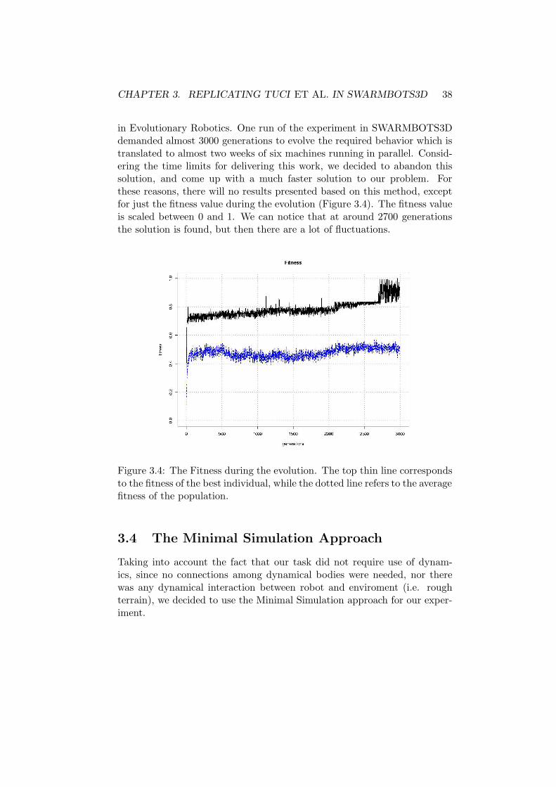
CHAPTER 3. REPLICATING TUCI ET AL. IN SWARMBOTS3D 38
in Evolutionary Robotics. One run of the experiment in SWARMBOTS3Ddemanded almost 3000 generations to evolve the required behavior which istranslated to almost two weeks of six machines running in parallel. Consid-ering the time limits for delivering this work, we decided to abandon thissolution, and come up with a much faster solution to our problem. Forthese reasons, there will no results presented based on this method, exceptfor just the fitness value during the evolution (Figure 3.4). The fitness valueis scaled between 0 and 1. We can notice that at around 2700 generationsthe solution is found, but then there are a lot of fluctuations.
Figure 3.4: The Fitness during the evolution. The top thin line correspondsto the fitness of the best individual, while the dotted line refers to the averagefitness of the population.
3.4 The Minimal Simulation Approach
Taking into account the fact that our task did not require use of dynam-ics, since no connections among dynamical bodies were needed, nor therewas any dynamical interaction between robot and enviroment (i.e. roughterrain), we decided to use the Minimal Simulation approach for our exper-iment.

CHAPTER 3. REPLICATING TUCI ET AL. IN SWARMBOTS3D 39
The robot and its world are once again simulated using a modified versionof the “minimal simulation” technique described by Jakobi in [32]. Jakobi’stechnique uses high levels of noise to guarantee that the simulated controllerwill transfer to a physically realised robot with no loss of performance. Ourhypothesis is that the controller will initially successfully transfer to theSWARMBOTS3D enviroment, when tested there. What we want to achieveis evolve the controller in a simple minimal environment, thus avoiding com-plicated dynamics relations which are not required according to the defini-tion of our task, acquiring the solution quickly and easily. Our hypothesiswill be confirmed if the robot behaves in a satisfactory manner, fulfilling thecriteria of correctly signalling and finding the way in zone, avoiding to makeerrors of any type—like crossing the band, when the evolved controller isdownloaded and tested on a physics-based simulator as SWARMBOTS3D.We will not demand that the robot moves identically in the two simulators,since that would be an extremely severe criterion, especially if the robot isable to carry out the task.
Therefore, we adapted the simulation of Tuci et al., modelling the Khep-era robot, so that it can model the fast s-bot model described in section 3.2.
The initial results were promising, but there was a big discrepancy in thebehavior of the robot in the SWARMBOTS3D enviroment and in the 2Dminimal simulator. Therefore, we had to come up with a way to compensatethe lack of dynamics in the evolutionary environmant. Jakobi claims thathigh levels of noise are required in order to expect a satisfactory tranfer ofthe controller to reality. Having already used noise on all sensorial informa-tion and on the robot’s position, we decided to also implement pink noiseon them. Pink noise is a way of avoiding the case where a system would“learn” the characteristics of the noise and thus its effect on the robustnessis reduced. In fact, what we do is ensure that the noise comes from differ-ent windows of the uniform distribution for each sensor and position. Also,there is a provision for long or short-term change to the sensor’s or position’svalue.
Another big change we had to implement was to adapt the positionupdating to the s-bot geometry. Initially we made use of the same look-uptable described in [32]—also used by Tuci et al., just altering the parameterswhich refer to the robot’s geometry and dimensions. Unfortunately theinitial results were not that satisfying, so we decided to use the kinematicsof a differential drive robot, as described by Dudek and Jenkin in [17].
The results were satisfactory in the sense that the robot was movingand behaving very similar to the Minimal 2D Simulator case. Of course,it is again of utmost importance to stress that we do not require the robot

CHAPTER 3. REPLICATING TUCI ET AL. IN SWARMBOTS3D 40
to behave identically in the two simulators, especially for what concernsits movement. This is almost impossible to achieve since a physics-basedenvironment contains interactions and dynamics that cannot be predicted.
The main lesson that we learned with the experimentation presentedabove is that if our task does not need physics to be achieved, we can usea Minimal simulation which can easily and fastly produce results, that cansuccessfully transfer to a physics-based environment, maybe even reality,with the use of noise.
The experiment we ran with the methodology described above is a repli-cation of the Tuci et al. experiment, with the Minimal Simulation approach.This allows us to spot possible differences in the results obtained, but isalso very encouraging since the experiment was successful, in our effort toproceed and expand their experiment. The post-evaluation is done in boththe Minimal 2D simulator and SWARMBOTS3D. Thus we will be able toinfer some conclusions on the success of the porting to the physics-based 3Dsimulator.
3.5 Results
3.5.1 The Replication
We made twenty replications of the experiments. Figure 3.5 shows the fit-ness of the best individual and the mean population fitness plotted againstthe generation number (5000) and averaged over the 20 replications. Wecan notice that in all replications of the experiment a successful behaviorwas evolved2. The 100% success rate can be accounted for by recalling thatthe fitness function, not rewarding any specific action except phototaxis andthe signalling behavior, has positively influenced the development of success-ful behaviors. In fact, evolution was left free to search for a strategy thatcould be effective for the achievement of the final goal. This was not thecase with the evaluation function used by Tuci et al., described in detail inSection 2.3.4. Their results report—after post-evaluation—12 out of 20 suc-cessful controllers. As we will show in Section 3.5.3, we obtained 18 out of 20successful controllers, that is controllers able to perform the discrimination.
2The maximum fitness value is almost 2, since for some of the controllers, the finalgeneration’s achieved fitness value is very close to 2 but not exactly 2

CHAPTER 3. REPLICATING TUCI ET AL. IN SWARMBOTS3D 41
Figure 3.5: Average fitness during the evolution. All plots are the averageover the 20 replications of the experiment. The top thin line corresponds tothe average fitness of the best individual, while the dotted line below refersto the average fitness of the population.
3.5.2 Analysis of the evolved behavioral strategies
A qualitative analysis of the evolved controllers confirms that a number ofdifferent behavioral strategies have been obtained. However, some constantcharacteristics can be recognised. At the beginning of a trial, all robotsperform phototaxis until they reach the circular band. When the grey levelon the floor overcomes a certain threshold, the robots start circuiting aroundthe light bulb with an approximately constant angular speed. Wheneverthe robots are placed in Env.A and the way in zone is detected, phototaxisstarts again and the light bulb is reached. On the contrary, in Env.B, aftertravelling on the band for a given time without detecting the way in zone,the robots initiate a signalling behavior.
An example of this behavior is shown in Figure 3.6: in both Env.A andEnv.B, it is possible to notice that, when the circular band is detected—seecontinuous line F at about simulation cycle 90—the robot starts moving onthe circular band maintaining a constant distance from the light bulb. Thisbehavior is indicated by the constant readings of the light sensors L1 and

CHAPTER 3. REPLICATING TUCI ET AL. IN SWARMBOTS3D 42
L2 and of the floor sensors F . In Env.A, the way in zone is encounteredshortly before simulation cycle 500, as indicated by the sudden drop in thefloor sensor F . At this point, the robot performs phototaxis again, rapidlyreaching the light bulb, as indicated by the high activation of the lightsensors L1 and L2 at the end of the simulation.
The constant angular speed on the circular band is the basic mecha-nism exploited for discrimination between Env.A and Env.B by successfullyevolved robots. In fact, this constant motion allows the robots to experi-ence a constant perceptual state (the grey level of the floor and the lightintensity that impinges on their sensors), which roughly corresponds to theconstant flow of time. In Figure 3.6, one can notice that the persistence ofa particular perceptual state, corresponding to the robot circuiting aroundthe light and over the band, makes the output S, which controls the sound,increase linearly. This perceptual state triggers the sound signalling throughan efficient integration mechanism which is based on the “feeling” of beingtravelling long enough over the circular band without having encounteredthe way in zone. In fact, if the way in zone is encountered, as in the upperpart of Figure 3.6, the activation of the neuron S decreases below the thresh-old level 0.5. This response makes the robot capable of avoiding to initiatethe signalling behaviour when it is not required. The situation is different inEnv.B: the absence of the way in zone let the output of neuron S reach andovercome the threshold level 0.5—see bottom part of Figure 3.6, simulationcycle 550. This response makes the robot capable of correctly signallingthat it is located in Env.B. It is also worth noticing that the output of theneuron S is rising in both enviroments, and around the same time in Env.Adrops—manifestating the detection of a way in zone—and in Env.B risesabove the threshold level. Finally, we can notice that the output of neuronS is initialised a bit below 0.5 and then drops linearly until the circular bandin shades of grey is discovered, when it starts rising again. This proves thatthe feeling of time is dependent of the previous experience of the robot, thatis of the distance it covered to reach the band. So in case it has to cover, forinstance, a bigger distance to reach it, the value of the neuron’s output willdecrease further on, possibly causing the robot to signal later the absenceof the way in zone, than it does for the initial distance.
In summary, the behavioral analysis revealed that the evolved controllersproduce the required sensory-motor coordination that brings forth a per-ceptual state that is integrated over time and exploited for discriminationthrough sound signalling.

CHAPTER 3. REPLICATING TUCI ET AL. IN SWARMBOTS3D 43
Environment type A
0
0.25
0.5
0.75
1
0 100 200 300 400 500 600 700
sens
or in
puts
L1L2F
0
0.25
0.5
0.75
1
0 100 200 300 400 500 600 700
outp
uts
simulation cycle
M1M2S
Environment type B
0
0.25
0.5
0.75
1
0 100 200 300 400 500 600 700
sens
or in
puts
L1L2F
0
0.25
0.5
0.75
1
0 100 200 300 400 500 600 700
outp
uts
simulation cycle
M1M2S
Figure 3.6: Behavioral analysis. The sensor activity and the correspondingmotor output are plotted for 700 simulation cycles. L1 and L2 refer to thelight sensors, while F refers to the floor sensor. M1 and M2 correspond tothe motors of the two wheels, and S refers to the sound signalling. When Sis bigger than 0.5, the robot emits a signal.
3.5.3 Post Evaluation in the Minimal Simulator Environ-
ment
In order to test the performance of the controllers evolved, it is required toperform a post evaluation. This is due to the possibility that the fitness of an

CHAPTER 3. REPLICATING TUCI ET AL. IN SWARMBOTS3D 44
evolved individual is overestimated. If this is the case, the post evaluationwill reveal it. Thus, we performed further analyses, by re-evaluating eachof the best evolved final generation individuals for 100 trials in each typeof environment (i.e., Env.A and Env.B). In each trial performed in Env.A,we look at the robot’s capability to reach the light bulb (Succ.), withoutincurring in any error. Errors can be of two types: E1 refers to the emissionof a sound signal, while E2 refers to crossing the black edge of the band.Similarly, in Env.B, we look at the performance of the robot on properlysignalling the absence of the way in zone (Succ.), without committing anyerror. Also in this case, two error types are possible: E3 refers to the lackof sound signalling, and E4 refers to the robot crossing the black edge ofthe band. Furthermore, in Env.B we also compute the offset between theentrance position of the robot in the circular band and the position in whichthe robot starts to signal. This measure, called offset ∆, is computed asfollows:
∆ = |α(te, ts)| − 2π, (3.4)
α(t1, t2) =
t2−1∑
t=t1
AOB, A = Xt,B = Xt+1 (3.5)
where O corresponds to the position of the light, and α is the angulardisplacement of the robot around the light from the starting position—theposition at time te when the robot enters into the circular band—to thesignalling position—the position at time ts when the robot starts signalling.Angular displacement α is computed summing up all the convex anglesAOB comprised between two consecutive position of the robot Xt, takinginto account that an angle is negative if the robot moves clockwise. Thismeasure accounts for the capability of a robot for searching the way in zone.Offset ∆ takes value 0 if the robot signals exactly after covering a completeloop of the circular band. Otherwise, it gives the angular displacement fromthis position. Negative values of the offset ∆ suggest that the robot signalsbefore having performed a complete loop, while positive values correspondto the situation in which the robot has performed more than one loop aroundthe light, waiting too long to signal.
Table 3.1 refers to the post-evaluation results. As we can see, 17 outof the 20 controllers perform well, having a very high success rate in bothEnv.A and Env.B. In general, 18 out of the 20 controllers are able to performthe discrimination task. It is worth noting that two of the controllers thatdo not perform well, both fail to signal in Env.B (replications 12 and 18).The errors of the rest of the controllers are mostly signalling errors (E1 and

CHAPTER 3. REPLICATING TUCI ET AL. IN SWARMBOTS3D 45
E3), while some replications of the experiments have a higher error ratein crossing the black edge of the circular band. This is due mainly to atendency of the robots to approach the black edge while circuiting on theband. Especially the controller in replication 11 has incured in this error lotsof times, making this controller almost unsuccessful in Env.B. Concerningthe offset ∆, most evolved controllers have a negative value, in general lowerthan 80 degrees, meaning that all robots signal before having completed oneloop of the circular band. However, this offset can enough to discriminatebetween Env.A and Env.B, as the way in zone is up to 90 degrees wide.Only in one case, in replication 1 and 13, the robot is “prudent”: that is, itsignals only after having completed a loop around the light bulb. The onlytimes the robot signals at an angle smaller than -90 degrees are replications11 and 18, which as we mentioned above are not successful. It is importanthere to remind the reader that our fitness function described in detail inSection 3.2.2 does not reward signalling exactly after a full loop, as the onein Tuci et al. did. Yet, we managed to produce more successful controllers,with the changes we implemented on some methodological issues.
3.5.4 Robustness of the evolved solutions
It is very important to acquire controllers that are able to adjust to varyingenviromental circumstances, that are able to display a satisfactory behavioreven in circumstances not encountered in evolution. As we criticized inSection 2.3.6, Tuci et al. fail to produce controllers able to do so. Onlyone out of the twenty controllers is able to display some generalization.Therefore, we decided to test the best evolved controllers of the twenty runsin an experimental setup where the distance between the light source and thecircular band varies between 20 and 60 cm, in Env.B. We measure the offsetof the robot as the forementioned distance varies. The results are diplayedin Table 3.2. In general we can say that the closer to the light source is thecircular band, the earlier the robot emits the sound. The distance that therobot has been travelling performing phototaxis until it reaches the blackband definitely plays a role in its subsequent behavior. The feeling of timetravelling in the band is not independent of the robot’s previous experience,that is the time it travelled to arrive to the band. This is a result of networkconfiguration and choice. Furthermore, if the band is positioned closer tothe light, the light sensors of the robot once upon the band are more active.We expect thus a different behavior if the robot is placed in an enviromentdifferent than the one in which it has been evolved. It is important to stressthe fact that the robot has not been evolved with a fitness function that

CHAPTER 3. REPLICATING TUCI ET AL. IN SWARMBOTS3D 46
Table 3.1: Post-evaluation. Performance of the ten best evolved controllers.The percentage of success (Succ. %) and the percentage of errors (E1, andE2 in Env.A, and E3, and E4 in Env.B, ) over 100 trials are shown forboth Env.A and Env.B. Additionally, the average offset ∆ and its standarddeviation (degrees) are shown for the environment type Env.B.
Post-Evaluation Results in the Minimal Simulation Environment
run Env.A Env.B
Succ. E1 E2 Succ. E3 E4 Offset ∆
(%) (%) (%) (%) (%) (%) Avg. Std
n. 1 78 0 1 100 0 0 16.40 45.03
n. 2 100 0 0 87 13 0 -8.15 47.90
n. 3 100 0 0 100 0 0 -47.86 9.83
n. 4 100 0 0 100 0 0 -78.99 14.58
n. 5 99 0 0 98 2 0 -28.89 17.44
n. 6 99 0 1 100 0 0 -71.84 25.91
n. 7 100 0 0 93 7 0 -19.97 15.62
n. 8 100 0 0 100 0 0 -28.41 15.49
n. 9 100 0 0 89 5 6 36.42 23.28
n. 10 100 0 0 100 0 0 -39.85 10.44
n. 11 100 0 0 54 8 38 -107.49 71.70
n. 12 89 0 0 0 100 0 -2.55 12.25
n. 13 100 0 0 98 2 0 30.24 19.72
n. 14 100 0 0 100 0 0 -21.40 12.55
n. 15 100 0 0 100 0 0 -1.16 22.41
n. 16 99 0 1 98 2 0 -0.62 37.90
n. 17 100 0 0 99 1 0 -58.19 25.39
n. 18 96 0 3 0 100 29 -102.57 57.72
n. 19 100 0 0 100 0 0 -36.10 7.95
n. 20 94 0 0 99 1 0 -68.15 19.32
would favor its signalling with zero offset.We can notice that there are a lot of controllers that are able to display
a good behavior, for a lot of distances, contrary to the results of Tuci et al.Of course, Tuci et al. present in their results smaller errors for the “bad per-forming” controllers, but we remind the reader here that our fitness functiondid not reward exact signalling. Another general remark is that in our re-sults they almost all fail when the band is positioned very close to the light,

CHAPTER 3. REPLICATING TUCI ET AL. IN SWARMBOTS3D 47
Table 3.2: Robustness analysis. Performance of the twenty best evolvedcontrollers. The average offset of 100 evolutionary runs is given for thementioned distances between the circular band and the light.
Robustness Analysis
run 20 25 30 35 40 45 50 55 60
1 495.88 375.90 183.21 62.28 18.13 -29.89 -149.03 -216.52 -228.68
2 -336.70 -346.56 -42.39 37.12 -12.90 -54.54 -41.04 -64.81 -83.73
3 -258.39 -219.49 -62.47 -18.30 -53.66 -78.09 13.97 -9.04 -27.20
4 -297.15 -343.73 -193.25 -32.21 -82.33 -134.39 -69.30 -66.60 -85.06
5 -346.36 -340.60 -101.55 11.76 -26.96 -49.27 -68.22 -81.20 -91.74
6 -43.15 20.76 15.44 -33.93 -72.28 -62.15 -74.20 -98.83 -118.44
7 -57.75 -79.16 72.67 22.70 -15.93 -46.20 -56.97 -73.77 91.81
8 -159.55 -182.58 -47.90 24.34 -30.34 -67.88 -32.55 -50.43 -65.23
9 432.50 312.10 167.09 83.69 35.01 1.09 11.06 -15.64 -38.37
10 82.22 69.18 43.91 -1.05 -36.29 -42.02 -57.71 -80.44 -99.29
11 -322.44 -332.44 -124.27 -68.14 -106.32 -150.58 -36.48 -55.62 -73.28
12 -356.13 -355.99 -355.74 -167.97 -3.38 -34.69 -79.94 -175.94 -200.85
13 -175.53 -242.47 -155.63 79.48 30.53 -10.77 17.36 -25.29 -54.62
14 -253.24 -41.58 57.42 12.09 -22.38 -41.10 -90.80 -103.97 -115.43
15 -74.19 -126.56 56.72 32.08 -0.30 -28.22 -36.15 -56.88 -96.15
16 263.80 225.88 163.90 57.61 -2.86 -47.91 -123.25 -139.07 -151.85
17 -348.21 -345.60 -282.34 -11.84 -63.76 -106.50 -138.68 -180.32 -203.69
18 8.37 -118.91 -65.88 -92.18 -108.91 -130.78 -169.82 -337.55 -341.41
19 -344.55 -344.31 -318.16 -1.67 -43.29 -80.16 -32.54 -51.80 -68.30
20 -308.60 -318.03 -13.27 -30.96 -69.84 -87.39 -50.85 -66.83 -79.52
namely 20 or 25 cm away from it. On the other hand, they seem to performvery well in distances bigger than the one for which they were evolved (40cm). Runs no. 2, 5, 7, 8, 10, 15, 19, 20 seem to perform well, especially fordistances bigger than 40 cm. It is possible that when the band is positionedvery close to the light, the light sensors activation is too high, affecting ina negative way the performance of the robot. What is also surprising isthat sometimes the controllers perform better for distances other than 40cm than for the latter distance. Finally, in Figure 3.7, we show the boxplotfor run 20, one of the most successful ones.
3.5.5 Post Evaluation in SWARMBOTS3D
In this section, we present the results obtained by post-evaluating inSWARMBOTS3D the best individual of the final generation of run no. 14,one of the most successfull ones, as we can see in Table 3.1. The robot was100% successful in both enviroments and had an average offset ∆ of -21.40degrees. As we mentioned in Section 3.1, the criteria for judging the qualityof the porting from the one simulator to the other must be relevant to the

CHAPTER 3. REPLICATING TUCI ET AL. IN SWARMBOTS3D 48
20 25 30 35 40 45 50 55 60
−30
0−
200
−10
00
100
light−band distance (cm)
offs
et (
degr
ees)
Figure 3.7: Robustness analysis for run no.20. The offset ∆ is plotted forvarying light-band distance. The box-plot shows 100 evaluations per box.Boxes represent the inter-quartile range of the data, while the horizontalbars inside the boxes mark the median values. The whiskers extends to themost extreme data points within 1.5 of the inter-quartile range from thebox. The empty circles mark the outliers.
task the robot has to carry out. We must not demand the robot to have anidentical behavior in the two very different simulators. Therefore, we willonce again perform a post-evaluation where we extract the same informa-tion as in Section 3.5.3, namely in Env.A the robot’s capability to reach thelight bulb (Succ.), without incurring in any error, errors E1 and E2 and forEnv.B, we look at the performance of the robot on properly signalling theabsence of the way in zone (Succ.), without committing any error and thetwo possible error types, E3 and E4. Furthermore, in Env.B we once againcompute the offset ∆.
The initial evaluations were performed with exactly the same settingsused in the Minimal Enviroment were the controller was also evolved. There-fore, we used the same initial orientation for the robot, thus between -120and 120 degrees (see Figure 2.1) and the same amount of timesteps for thelifetime of the robot, so 700. The initial results were quite disappointing.What we found out was that due to acceleration, inertia and friction, the

CHAPTER 3. REPLICATING TUCI ET AL. IN SWARMBOTS3D 49
robot lost a lot of time trying to orient itself correctly towards the light andthen perform phototaxis. In fact, the robot moved towards the light bulbin both simulators with his back turned to the light. This is the solutionevolution found for our problem. Therefore, placing the robot in a positionfacing the light, even with some variability, caused a spinning of the robotin order for the correct orientation to be found and then for phototaxis tobe performed. Of course, this was also the case in the Minimal Simulatorenviroment, but in this case, the acceleration, inertia and friction seemed tocause a very annoying delay in the beginning of the robot’s lifetime. In orderto confirm our hypothesis that the initial orientation matters, we conductedthe same evaluation for three different configurations:
• orientation π: the robot is placed in a position facing the light, themost inappropriate for phototaxis
• orientation π+[-120,120]: the robot is placed in the original orientation
• orientation 0: the robot has its back turned to the light, having themost appropriate orientation for phototaxis.
As we can see in Table 3.3, our hypothesis was confirmed. The robotperformed well only in the latter of the three cases, behaving extremely badfor the π orientation.
Looking at the results for the robot facing the light, we see that it wasnot able to signal in any of the 100 trials. Looking at the behavior ofthe simulated robot, it was obvious that because of the totally unfavorableinitial orientation and the disruptive effect of dynamics in the phase wherethe robot tried to find a suitable orientation to perform phototaxis, therobot’s lifetime was not enough for it to perform a complete loop aroundthe light and thus discriminate between the two enviroments, thus emittinga sound. Therefore, we decided to perform some more experimentation,this time varying the timestep value, from the initial 700 value up to itsdouble, 1400. As we can see in Table 3.3, the performance of the robotimproves significally if its lifetime is increased above 800 timesteps, even forunfavorable initial orientations.
The conclusions we can draw from this post-evaluations is that it ispossible to compare the results obtained in the two enviroments, but wehave to be very careful because the influence of parameters that are notso important in the Minimal Simulation case, like the initial orientation, isaffected by dynamics. Since that must be a value that is identical whenwe make a comparison between the two series of results, we have to give
CHAPTER 3. REPLICATING TUCI ET AL. IN SWARMBOTS3D 50
the robot a longer lifetime if evaluated in the SWARMBOTS3D simulator.We can see that the performance is definitely comparable to the one in theMinimal Simulator case. What is also astonishing is the fact that the robotnever crosses the black band in this case too, which is due to the noise on thefloor sensor, the bigger proportion of Env.A encountered during evolutionand the varying amplitude of the way in zone. Finally, the average offset∆ value is almost identical to the one obtained in the post-evaluation withthe Minimal Simulator. This is almost a surprising result which proves thatindeed the only discrepancy present between the two simulated behaviorslies in the initialisation of the robot and the effect of 3D dynamics andkinematics in its repositioning—which can be minimized by allowing therobot to live longer in the 3D case.

CHAPTER 3. REPLICATING TUCI ET AL. IN SWARMBOTS3D 51
Table 3.3: Post-evaluation in SWARMBOTS3D. The percentage of success(Succ. %) and the percentage of errors (E1, and E2 in Env.A, and E3,and E4 in Env.B, ) over 100 trials are shown for both Env.A and Env.B.Additionally, the average offset ∆ and its standard deviation (degrees) areshown for the environment type Env.B. These values are displayed for vari-ous timesteps and initial robot orientations.
Post-Evaluation Results in SWARMBOTS3D
orientation timestep Env.A Env.B
Succ. E1 E2 Succ. E3 E4 Offset ∆
(%) (%) (%) (%) (%) (%) Avg. Std
0 700 93 0 0 88 12 0 -22.59 34.90
0 800 100 0 0 95 3 0 -21.07 34.52
0 900 100 0 0 96 3 0 -20.95 34.56
0 1000 100 0 0 95 0 0 -20.95 34.56
0 1100 100 0 0 92 1 0 -20.95 34.56
0 1200 100 0 0 82 0 0 -20.95 34.56
0 1300 100 0 0 79 3 0 -20.95 34.56
0 1400 100 0 0 71 0 0 -20.95 34.56
π 700 62 0 0 0 100 0 - -
π 800 65 0 0 59 41 0 -15.52 46.97
π 900 93 0 0 92 4 0 4.13 25.24
π 1000 96 0 0 98 1 0 5.72 18.19
π 1100 97 0 0 94 0 0 5.89 17.48
π 1200 99 0 0 94 0 0 5.89 17.48
π 1300 99 0 0 87 0 0 5.89 17.48
π 1400 99 0 0 86 1 0 5.89 17.48
π+[-120,120] 700 94 0 0 58 40 0 -7.43 38.94
π+[-120,120] 800 100 0 0 93 5 0 0.47 33.5
π+[-120,120] 900 100 0 0 98 0 0 1.93 31.87
π+[-120,120] 1000 100 0 0 95 0 0 1.93 31.87
π+[-120,120] 1100 100 0 0 93 0 0 1.93 31.87
π+[-120,120] 1200 100 0 0 87 0 0 1.93 31.87
π+[-120,120] 1300 100 0 0 80 1 0 1.93 31.87
π+[-120,120] 1400 100 0 0 72 2 0 1.85 31.72

Chapter 4
Evolving communicating
agents that integrate
information over time
In this chapter we present a second set of experiments we conducted, ofa much more complicated nature. Two s-bots have to integrate over timetheir perceptual experience and communicate the result to the other robot,resulting in a cooperative behavior. The robot that has first finished itsintegration of its perceptual state must inform the other member of thegroup—in case of absence of a way in zone, by signalling. Therefore, theactions of each robot are now affected by the perceptual state of the othermember of the group. Finally, the robots are required to adjust their strategyafter a signalling behavior has been triggered by either robot and go awayfrom this inaccessible light source. It is important to notice that the latterbehavior is reactive, since the robots simply react to an enviromental signal.
Evolution must find a solution by evolving a single neural network thatcontrolls two robots, which must successfully alternate between reactive andnon-reactive behaviors. Furthermore, the controller should be able to dis-play even contradictory behaviors, that is going towards and away from thelight source. Finally, the robots should quit their current activity and pur-sue another, once the communication signal is transmitted. These pointsillustrate the difficulties and challenges of the task.
We present in detail the simulation, the evolutionary algorithm, the neu-ral controller and the evaluation function used for this experiment and in theend we present and analyse the results obtained. Furthermore, we compareonce again the post evaluation results obtained with the Minimal Simulation
52

CHAPTER 4. EVOLVING COMMUNICATING AGENTS 53
approach with the ones obtained in SWARMBOTS3D.
4.1 The Task
This task is inspired by two distinct sources. The first one is the finalscenario depicted in Figure 1.3 and described in [15]. A desired property ofan explorer robot is to be able to communicate to the other members of theswarm the results of his search. More specifically, in case a trough is detectedby a robot, this robot should inform the swarm about the nature of thetrough, so if it can be traversed by a single s-bot or if there is a way in zone,in order to pass to the other side. Since we have to allocate our resourcesin the best possible way to achieve an optimal use of the number of s-botsavailable, we want to avoid having more than one robots reaching to the sameconclusions about the same part of the explored enviroment. The secondsource of inspiration is biology. Animals that forage in a heterogeneousenvironment, where resources are distributed in patches, are required tomake “complex decisions” such as the patch in which to forage, and atwhich moment in time it is better to leave and travel to another patch.To make such decisions, animals need to acquire relevant information fromtheir environment. Afterwards, through stigmergic or direct communicationthey communicate their decision to the other members of the colony. Ageneral problem common to biology and robotics concerns the definition ofthe mechanisms necessary to decide when it is better to pursue a particularaction in a certain location and at which moment in time it is better to leavefor pursuing a similar or a different activity in a similar or different location.
Once again, we are going to make use of the Minimal Simulation ap-proach. This time though, we have to overcome certain obstacles. Since tworobots are present in the enviroment, we are probably going to face collisionsbetween them. A physics-based 3D simulator can take care of the collisionssince the two robots are modelled like dynamical bodies. In our MinimalSimulation approach we are not using any forces, therefore we have to evolverobots that can perform obstacle avoidance, thus avoiding the other robot.In order to be able to do this, we have to use simulated proximity Infra-Redsensors, along with the other sensors used also in the Tuci et al. experiment,so that the robots can “sense” each other. The robots perceive the lightthrough their ambient light sensors, positioned 45 degrees left and 45 de-grees right with respect to their heading. Light levels alter depending on therobots distance from the light. The colour of the arena floor is once againwhite, except for a circular band, centered around the lamp, within which

CHAPTER 4. EVOLVING COMMUNICATING AGENTS 54
the floor is in shades of grey. The circular band covers an area between40 cm and 60 cm from the light; the floor is black at exactly 40 cm fromthe light; the grey level decreases linearly with the distance from the light.Again the robots perceive the colour of the floor through their floor sensor,positioned on their bellies, which outputs a value scaled between 0—whenthe robots are positioned over white floor—and 1—when they are over blackfloor. The robots are also equipped with a sound sensor, which is binaryand is set to 1 if any robot is signalling (including the robot itself), and to0 if no robot is signalling. This sensor will implement communication.
Concerning the robot’s controller, this time we decided not to use moreneurons than the sum of inputs and outputs of the network, as was done byTuci et al.. The reason is that with the use of IR proximity sensors and theextra communication sound sensor, the network has become already quitebig. Therefore, it will be harder for evolution to find the solution, giventhat the search space has singifically grown. So, our genotype is a vectorcomprising 144 real values (121 connections, 11 decay constants, 11 biasterms and a gain factor).
At the beginning of each trial, two simulated s-bots are positioned withina boundless arena, one of them at about 85 cm west of the light bulb, with arandomly determined orientation chosen between north-east and south-east(see Figure 2.1 left), and one at about 115 cm west of the light bulb, withthe same random orientation.
Similar to Tuci et al., there are two types of environment. In Env.A theband presents a discontinuity—a way in zone (see Figure 2.1, left). In Env.Bthe band completely surrounds the light (see Figure 2.1, right). The way inzone represents the path along which the robots are allowed to safely reachthe light in Env.A. Successful robots should prove capable of performingphototaxis as well as looking for the way in zone, avoiding to cross theblack edge of the band. Such robots should always reach the light in Env.A,avoiding crashing with each other. On the contrary, in Env.B, the robotsshould, besides avoiding to cross the black edge, signal the absence of theway in zone by emitting a tone. Furthermore, they have to react to thelatter signal—no matter from which robot it came from— and move awayfrom this light source which does not present a way in zone.
4.2 The Simulation
During the evolution, each genotype is coded into a robot controller, andis evaluated 15 times, 12 times in Env.A and 3 times in Env.B. We use

CHAPTER 4. EVOLVING COMMUNICATING AGENTS 55
this proportions once again, as they led to more robust controllers in thereplication of the Tuci et al. experiment. At the beginning of each trial, theneural network is reset—i.e., the activation value of each neuron is set tozero. Each trial differs from the others in the initialisation of the randomnumber generator, which influences the robots’ starting position and orien-tation, the position of the way in zone, and the noise added to motors andsensors. For each trial in Env.A, the position of the way in zone is variedto facilitate the evolution of robust navigational strategies. Its amplitudevaries within the interval [π
6, π
2]. Once, again we choose a varying amplitude
since it contributed to obtaining more robust controllers in our replicationof Tuci et al.. Within a trial, the robot life-span is 280 seconds (1400 sim-ulation cycles). A trial is terminated earlier if both robots cross the blackedge of the band (see dashed arrows in Figure 2.1) or because both reach anEuclidean distance from the light higher than 140 cm. In each trial e, therobots are rewarded by the average of the values of the fitness function ofthe two robots. This way we ensure that in order to result in a successfulbehavior, both robots must perform well.
In case the robots are situated in Env.A, they are each rewarded byfunction fe1 which corresponds to the sum of the following two components:
1. Rmotion—This component rewards movement toward the light bulb,and it is computed as:
Rmotion =di − df
di(4.1)
where di and df represent respectively the initial and the final Eu-clidean distance between the robot and the light bulb. In Env.A, df
is set to 0 if the robot is less than 15 cm away from the light bulb.
2. Rsignal—This component rewards agents that do not signal. The com-ponent is computed as:
Rsignal =
{
1 if no signalling0 otherwise
(4.2)
In case the robots are situated in Env.B, they are each rewarded byfunction fe2 which corresponds to the sum of the following two components:
1. Rmotion—This component rewards movement toward the light bulb,if none of the robots have signalled, and moving away from the lightbulb if any of the two robots has signalled. It is computed as:

CHAPTER 4. EVOLVING COMMUNICATING AGENTS 56
Rmotion =
{
di−df
diif no robot has signalled
df
dmaxif any robot has signalled
(4.3)
where di and df represent respectively the initial and the final Eu-clidean distance between the robot and the light bulb and dmax is themaximum distance the robot is allowed to go away from the light.This will ensure that the robots will go away from the light after oneof them has emitted a sound communicating that there is no way inzone, and reach a distance from it equal to 140 cm for this simulation.Df is set to 0 when the robot is on the circular band in shades of grey.
2. Rsignal—This component rewards agents that signal. The componentis computed as:
Rsignal =
{
1 if any robot signalled0 otherwise
(4.4)
Notice that the evaluation function used is identical to the one used inSection 3.2.2 (equation 3.2), when the robots are located in Env.A. On theother hand, if the robots are situated in Env.B, Rmotion is different in thesense that if any of the two robots has signalled, it changes and insteadof rewarding phototaxis, it rewards the opposite behavior. Also, Rsignal isdifferent in the sense that each robot does not only get rewarded by its ownaction of emitting a sound, but also by the other group member’s action. Theevaluation function described above is very simple, being the least explicitpossible. Even though component Rsignal for Env.B could be made moreexplicit punishing robots that both finish the loop and signal, ignoring thecommunication signal, we let evolution free to explore the search space,which for this experiment is very big.
In order to evolve robot-robot avoidance, we punish the robots wheneverthey approach each other below a critical distance. The more the robotsfall into thar error during their lifetime, the more they are punished. Themaximum number of virtual crashes we allow is set to 3 and above thisvalue the robots die being punished very severely, rewarded very poorly bythe evaluation function. Since they are initialised quite far from each otherin order to ensure that one of them will be able to finish its integrationearlier than the other and signal first—in Env.B—, the only time the robotsreally interact is when they are located in Env.A and very close to the light—having both found the way in zone. We let the robots interact in this areafor a long interval in order to ensure that they evolve robot-robot avoidance.

CHAPTER 4. EVOLVING COMMUNICATING AGENTS 57
4.3 Results
We ran 10 evolutions, each with a different random initial seed, for 5000generations. In eight of them, the maximum fitness value of around 2 wasachieved. Two runs did not find the solution, and evolution was stuck at apoint where the robots fail to signal the absence of a way in zone. Figure 4.1shows the fitness of the best individual and the mean population fitnessplotted against the generation number (5000) and averaged over the 10replications. We can notice that the average fitness of the best individuals ofall replications is slightly over 1.9, which is normal if we take into account thefact that the two unsuccessful controllers had a fitness of 1.8. Of course, post-evaluation will reveal once again if some controllers were lucky in obtainingthe maximum fitness value and if there are drawbacks in their behavior.
Figure 4.1: The Fitness during the evolution. The top thin line correspondsto the fitness of the best individual, while the dotted line refers to the averagefitness of the population.
4.3.1 Post-Evaluation in the Minimal Simulator
In order to test the performance of the controllers evolved, it is required toperform a post evaluation. This is due to the possibility that the fitness of an

CHAPTER 4. EVOLVING COMMUNICATING AGENTS 58
evolved individual is overestimated. If this is the case, the post evaluationwill reveal it. Especially in our case, sometimes the robots might havebeen lucky without ever crashing against each other during their lifetime, orwithout ever crossing te black edge. Thus, we performed further analyses,by re-evaluating each of the best evolved final generation individuals for 100trials in each type of environment (i.e., Env.A and Env.B). In each trialperformed in Env.A, we look at the two robots’ capability to both reachthe light bulb (Succ.), without incurring in any error. Errors can be of twotypes, for each robot: E1 refers to the emission of a sound signal and E2refers to crossing the black edge of the band. The results are displayed inTable 4.1. In Env.B, we look at the performance of the two robots in thefollowing way: We measure the times the complete task is successful, that isthe first robot to reach the band properly signals the absence of the way inzone and then both robots leave the grey zone and end up in a distance of140 cm away from the light source, without committing any errors (Succ.).We also measure the reaction time for each robot (react), that is the numberof timesteps required by each robot to get out of the circular band in shadesof grey in order to go away from this light source. In this case, three errortypes are possible: E3 refers to the lack of sound signalling by the first robot(we do not care if the second robot signals or not), E4 refers to the robotscrossing the black edge of the band and E5 for each robot refers to the timesthey end up at a different distance from the light source than the desiredvalue of 140 cm. Finally, in Env.B we also compute the offset between theentrance position of the robot arriving to the circular band first and theposition in which this robot starts to signal. This measure, called offset ∆,is computed as in equation 3.4. The results are displayed in Table 4.2.
We can see from the results that it was not an easy task for evolutionto find a solution for our task. Especially the fact that we require therobots to perform both phototaxis and go away from the light, and thosecontradictory behaviors to be both displayed by the same controller makesthe task difficult. Evolution has to shape one single neural network for tworobots that manage to display a very robust transition between reactive andnon-reactive behaviors. Robots are also required to rapidly quit their currentaction and switch to another once they hear a communication signal emittedby the other member of the group. Nevertheless, evolution managed to findfour controllers, namely the ones produced in runs no. 3, 7, 8 and 10 thatperform very well. The errors are very few and the Succ. rate is high andcould have been almost maximal if the robots did not crash sometimes whenlocated in the vicinity of the light source in Env.A. Of course, these crashesare virtual and it would be better to use the expression of approaching each

CHAPTER 4. EVOLVING COMMUNICATING AGENTS 59
other more than a critical distance. It is worth noting at this point thatin almost all runs we have some crashes, but it is rather difficult to evolverobots that are required to be both in a distance smaller than 15 cm fromthe light source, given that their diameter is already 5.8 cm. Reaction timefor the latter controllers is quite small and the average value of the offset∆ is excellent for runs no. 7 and 8, good for run no. 3 but big for runno. 10, since the way in zone’s amplitude varies up to 90 degrees. Also,the robots almost always end up in the desired distance from the light, thatis the number of E5 is very low. Runs no. 2 and 6 perform fine, but thenumber of E4 and E5 is rather high. Run no. 4 is unsuccessful, but lookingat the evolved behavior in our simulated 2D environment we found out thatevolution found a solution that under some circumstances was evaluatedwith the maximum score, despite the fact that it was not optimal. Therobots signal before reaching the black band, and then immediately gofurther away from the light source, reaching the distance they are supposedto, in all trials in Env.B. Also, in Env.A, we can see that in many trialsthe robots erroneously emit sound. Finally, the fact that it is hard forevolution to shape a network able to display two contradictory behaviors—going towards and away from the light—is illustrated in the results of runno. 5. The performance is optimal, except for the fact that the robots inall cases fail to reach the desired distance from the light (140 cm). On thecontrary, they start spinning at a smaller distance to it and afterwards thegoing away behavior is disrupted.
Concerning communication, it is evident that in the vast majority ofthe cases the robots react very quickly to the signalling. Notice that wemeasure the simulated timesteps they spend to go out of the circular bandin shades of grey. An average of 45 timesteps corresponds to 4.5 seconds toleave the black band, which is a very fast reaction. We remind the readerthat the robots are required to disrupt their action of looping around thelight staying inside the grey circular band and then signalling the absenceof a way in zone. They must pursue a very different action from that pointon, which is not based on constant light readings anymore (see Section 3.5.2and Figure 3.6).
Finally, regarding the times the robots cross the black band, we noticethat in our experiment, this number is higher than in the replication of Tuciet al.. One explanation for this is that the robots are initialised with anaverage distance of 30 cm between them. As we saw in Section 3.5.4, thedistance to the lights for which the robots are evolved is crucial, and whenplaced in varying distances, their performance—in general—drops. In ourcase, one single network should control two robots that must perform the

CHAPTER 4. EVOLVING COMMUNICATING AGENTS 60
same task, but under very different conditions. The distance the one robotmust cover in order to reach the circular band in shades of grey is muchbigger than the one the other has to cover.
Table 4.1: Post-evaluation in the Minimal Simulation environment. Per-formance of the ten best evolved controllers in Env.A. The percentage ofsuccess (Succ. %) and the percentage of errors E1 and E2 over 100 trials areshown for both robots. Robot 1 is initialised closer to the light source.
Post-Evaluation Results inthe Minimal Simulation Environment
Env.A
run Succ. E1 E2
r1 r2 r1 r2
(%) (%) (%) (%) (%)
n. 1 85 0 0 0 0
n. 2 92 0 0 0 0
n. 3 88 0 0 1 0
n. 4 62 31 31 3 4
n. 5 94 0 0 0 0
n. 6 98 0 0 1 1
n. 7 76 0 0 0 0
n. 8 94 0 0 1 0
n. 9 94 0 0 0 0
n. 10 92 0 0 0 0
4.3.2 Post-Evaluation in SWARMBOTS3D
As we did in Chapter 3 and with the replication of the Tuci et al. experiment,we are interested in re-evaluating the controllers evolved in the MinimalSimulation environment in SWARMBOTS3D. To do so, we will extract thesame information as in Section 4.3.1. We re-evaluate 100 times again inEnv.A and 100 times in Env.B the best controllers of run no. 10, one ofthe most successful runs over all. In Table 4.3 we can see the results of thepost-evaluation in Env.A, and in Table 4.4 the results for Env.B.
As we can see, in Env.A, the controller controllers behaves in a verysimilar manner in both simulators (see also Table 4.1). The success rate ishigh in both cases and the number of errors is almost identical. Again, thecases where the robots do not succeed usually are caused by crashes around

CHAPTER 4. EVOLVING COMMUNICATING AGENTS 61
Table 4.2: Post-evaluation in the Minimal Simulation environment. Per-formance of the ten best evolved controllers in Env.B. The percentage ofsuccess (Succ. %), the reaction time, the percentage of errors E3, E4 andE5 over 100 trials are shown for both robots. Additionally, we show theaverage offset ∆ and its standard deviation (degrees) for the first robot thatcompletes the loop. Robot 1 is initialised closer to the light source.
Post-Evaluation Results in the Minimal Simulation Environment
Env.B
run Succ. react E3 E4 E5 Offset ∆
r1 r2 r1 r2 r1 r2 Avg. Std
Avg. Std Avg. Std
(%) (%) (%) (%) (%) (%) (%) (%) (%) (%)
1 0 — 100 0 0 —
2 50 96.9 51.7 104.13 50.02 0 21 30 2 2 -86.71 54.86
3 95 65.23 25.98 67.02 28.98 0 2 3 0 0 -71.30 89.29
4 0 — 0 7 8 5 4 —
5 0 113.17 35.62 118.13 29.12 0 0 0 100 100 -28.45 67.95
6 67 60.61 48.26 61.68 41.81 6 4 16 9 3 0.59 119.68
7 96 45.04 83.97 38.30 13.14 1 0 0 2 1 -30.34 122.50
8 90 46.31 11.29 45.98 10.53 1 3 5 1 0 -27.36 90.08
9 0 — 100 0 1 —
10 100 74.1 17.67 73.8 16.58 0 0 0 0 0 -113.74 98.64
the light source, after the way in zone is found by both robots.In Env.B though, things are not that similar (see also Table 4.2). The
success rate is again 100% no errors are made, the reaction time is almostidentical, but we see a very big discrepancy in the value of the offset ∆.When re-evaluated in the minimal simulator environment, the robot ini-tialised closer to the band was signalling on average too early. On the otherhand, when re-evaluated in SWARMBOTS3D, it is signalling too late. Forreasons discussed in Section 3.5.5, the initial orientation of the robots, beingπ+[-120,120], is disrupting phototaxis and causes a lot of problems in thephysics-based 3D environment. Also, as we saw in Section 4.3.1, the factthat the robots are initialised with an average distance of 30 cm betweenthem, affects their performance. More specifically it is more difficult for therobot to reach the band first, to signal at the right moment the absenceof a way in zone, since one single network should control two robots thatmust perform the same task, but under very different conditions. If we takeinto account the disruptive effect of dynamics in the phase where the robotshave to adjust their orientation and perform phototaxis, we can explain thevery big discrepancy in the values of the offset ∆ in the two simulated envi-

CHAPTER 4. EVOLVING COMMUNICATING AGENTS 62
ronments. Finally, as mentioned in Section 3.5.5, the feeling of time is notindependent of the previous experience, that is the robot’s memory whileon the band is affected by the time it has been moving to get there.
It is clear that this time it is much more challenging to acquire similarresults when testing an evolved controller in the two simulated environments.In this complex task we have to use parameters that worsen the performanceof the controller in the physics-based 3D environment, like the difference inthe initial distances. It is possible that modifying some parameters—like wedid in Section 3.5.5—might lead to more consistent results. But this studyis out of the scope of this work and was not performed.
Table 4.3: Post-evaluation in SWARMBOTS3D. Performance of one evolvedcontroller in Env.A. The percentage of success (Succ. %) and the percentageof errors E1 and E2 over 100 trials are shown for both robots. Robot 1 isinitialised closer to the light source.
Post-Evaluation Resultsin SWARMBOTS3D
Env.A
run Succ. E1 E2
r1 r2 r1 r2
(%) (%) (%) (%) (%)
n. 10 89 0 0 0 0
Table 4.4: Post-evaluation in SWARMBOTS3D. Performance of one evolvedcontroller in Env.B. The percentage of success (Succ. %), the reaction time,the percentage of errors E3, E4 and E5 over 100 trials are shown for bothrobots. Additionally, we show the average offset ∆ and its standard de-viation (degrees) for the first robot that completes the loop. Robot 1 isinitialised closer to the light source.
Post-Evaluation Results in SWARMBOTS3D
Env.B
run Succ. react E3 E4 E5 Offset ∆
r1 r2 r1 r2 r1 r2 Avg. Std
Avg. Std Avg. Std
(%) (%) (%) (%) (%) (%) (%) (%) (%) (%)
10 100 69.86 1.03 58.40 8.50 0 0 0 0 0 72.62 14.00

Chapter 5
Conclusions
In this work we addressed the problem of defining the control system for agroup of autonomous robots that have to deal with a non-reactive task. Wesuccessfully designed neural controllers for robots that integrate over timetheir perceptual experiences in order to initiate alternative actions. We madeuse of techniques derived from Artificial Evolution, and we showed how theycan produce simple but effective and robust solutions. One of the interestingpoints that came up during our experiments was the problem of choosing thenature of the simulator in which we evolved our controllers, having to choosebetween a 3D physics-based environment taking into account dynamics andforces, and a Minimal Simulator—a much faster method. The latter solu-tion was chosen since our task did not require forces in order to be solvedand since we proved that with the correct modifications, the controllers itproduces can perform equally well in a realistic simulated enviroment.
5.1 Results
We ran two sets of experiments. The first one was a replication of the ex-periment of Tuci et al., in order to port its results in the SWARM-BOTSproject context. In this experiment, a robot must integrate over time itsperceptual experience, thus “feeling” the flow of time. Changes in variousmethodological aspects were made in order to produce more robust solutionsand better-performing controllers. Initially, we tried to evolve the controllersin a physics-based 3D enviroment, but since this method was not efficientenough as far as time and computational power are concerned, it was aban-doned. We turned to the Minimal Simulation approach, which was ableto rapidly produce robust solutions. These solutions were able to perform
63

CHAPTER 5. CONCLUSIONS 64
equally well when tested in a realistic simulated environment, revealing thepower of the Minimal Simulation approach.
The second experiment was an extension of the latter experiment, moresuited for a collective robotics scenario. Two robots were able to integrateover time their perceptual experience and communicate the result to theother member of the group, resulting in an alternative action. The simu-lated robots managed to display a very robust transition between reactiveand non-reactive behaviors. Once again, we used the Minimal Simulationapproach.
One of the major achievements of this work is the fact that we managedto design one controller able to display a very complex behavior. Thecontroller can trigger even contradictory behaviors, namely phototaxis andgoing away from the light source, depending on a decision it has to make.Robots can also rapidly quit their current action and switch to anotheronce they hear a communication signal emitted by the other member of thegroup. Of course, there are other ways of designing a control system forrobots having to perform the task we described, like hand-crafting parts ofthe solution. We cannot prove that our approach is better, but we provedthat our approach was successful, even though it is time-consuming and nottrivial to synthesize an integrated (not modularised) neural network throughan evolutionary process. Our contribution to the literature is that we showedthat evolution can produce robust solution for a complex task like the onewe described.
This experiment finally is a very important first step towards the real-ization of a complex SWARM-BOTS project scenario. We have designeda decision-making mechanism that with the use of communication will bevery useful to the swarm-bot, since the s-botswill often be required to makecomplex decisions based on their perception of the environment.
5.2 Future Work
Our work can be extended in various directions. The first and most obviousis a collective robotics one, like the task the swarm-bot has to carry outin the scenario described in [15]. It would be of particular interest to haverobots that are able to aggregate or self-assemble after one of them realisesthat the trough it discovered cannot be traversed by one robot. Also, ifthe knowledge every robot gathers about its environment is communicated,we will have a better allocation of resources, exploiting the s-bots moreefficiently. Another direction is more biology-inspired, specifically by patch

CHAPTER 5. CONCLUSIONS 65
foraging. It would be interesting to see if robots that leave a light sourcethat is not accessible can locate and approach other, accessible light sources,by exploring their environment. The inspiration is animals that leave a foodsource they cannot exploit and look for others in their environment. Finally,we could also move in the direction of exploring the use of communication.If the sound sensor is made distance or direction-dependent, we can be ableto coordinate the movement of the two robots in various manners, enrichingthe repertoire of behaviors they can exhibit.
Nevertheless, as in any robotics study, the ultimate challenge is to beable to port the results obtained in simulation on real robots. In order tobe more confident that we will be successful, we have to perform some fur-ther experimenting and apply several changes. Sensorial information mustbecome more realistic, especially concerning the sensor that encodes thestatus of the enviromental cue used for discrimination between different en-viroments, that is the floor sensor, and the sound sensor that implementscommunication between the robots. The floor sensor can be one of the 15infra-red proximity sensors mounted on the real s-bot. The sound sensorcan be one or a combination of the four sound sensor mounted on the s-bot.Furthermore, the simulated robot model used has to be closer to reality.Since the SWARMBOTS3D simulator provides a detailed simulated s-botwhich models very closely the real robot, we will run our experiments withthat model. Finally, methodological aspects during evolution might needreconsideration in order to achieve more robustness. Specifically, we wouldlike to make the “feeling of time” independent of previous—irrelevant tothe task—experience, but only dependent of the environmental cue used fordiscrimination.

Bibliography
[1] D.H. Ackley and M.L. Littman. Interaction Between Learning andEvolution. In Proceedings of the Second Conference on Artificial Life,pages 487–507, New York, USA, 1991. Addison-Wesley.
[2] W. Agassounon, A. Martinoli, and R.M. Goodman. A Scalable, Dis-tributed Algorithm for Allocating Workers in Embedded Systems. InProc. of the IEEE Conf. on System, Man and Cybernetics SMC-01,pages 3367–3373, Piscataway, NJ, October 2001. IEEE Press.
[3] T. Balch and R.C. Arkin. Communication in Reactive MultiagentRobotic Systems. Autonomous Robots, 1(1):27–52, 1994.
[4] G. Baldassarre, S. Nolfi, and D. Parisi. Evolution of Collective Behaviorin a Team of Physically Linked Robots. In Proceedings of EvoROB2003,Essex, UK, April 2003.
[5] R. D. Beer. A Dynamical Systems Perspective on Agent-EnvironmentInteraction. Artificial Intelligence, 72:173–215, 1995.
[6] R. D. Beer. On The Dynamics of Small Continuous-Time RecurrentNeural Networks. Adaptive Behavior, 3(4):471–511, 1995.
[7] R.D. Beer and J.C. Gallagher. Evolving Dynamical Neural Networksfor Adaptive Behavior. Adaptive Behavior, 1:91–122, 1992.
[8] J. Blynel and D. Floreano. Exploring the T-Maze: Evolving Learning-Like Robot Behaviors using CTRNNs. In G. R. Raidl et al., editor,Applications of Evolutionary Computing, EvoWorkshops2003, volume2611 of LNCS, pages 598–609. Springer-Verlag, Berlin, Germany, 2003.
[9] A. Bonarini and V. Trianni. Learning Fuzzy Classifier Systems forMulti-Agent Coordination. Information Science, 136:215–239, 2001.
66

BIBLIOGRAPHY 67
[10] R. Brooks. Intelligence Without Representation. Artificial Intelligence,47:139–159, 1991.
[11] R. A. Brooks. Intelligence Without Reason. In J. Mynlopoulos andR. Reiter, editors, Proceedings of the 12th International Joint Confer-ence on Artificial Intelligence, San Mateo, 1991. CA: Morgan Kauf-mann.
[12] D. J. Bruemmer, D. D. Dudenhoeffer, M. O. Anderson, and M. D.McKay. A Robotic Swarm for Spill Finding and Perimeter Formation.In Proceedings of International Conference on Nuclear and HazardousWaste Management (Spectrum), Reno, NV, USA, 2002.
[13] A. Castano, W. Shen, and P. Will. CONRO: Towards Deploy-able Robots with Inter-Robot Metamorphic Capabilities. AutonomousRobots, 8:309–324, 2000.
[14] G.S. Chirikjian. Kinematics of a Metamorphic Robotic System. InE. Straub and R. Spencer Sipple, editors, Proceedings of the Interna-tional Conference on Robotics and Automation. Volume 1, pages 449–455, Los Alamitos, CA, USA, May 1994. IEEE Computer Society Press.
[15] M. Dorigo. Wp5: Project Demonstration Scenario. Technical report,SWARM-BOTS PROJECT, 2004.
[16] M. Dorigo, V. Trianni, E. Sahin, R. Groß, T. H. Labella, G. Baldas-sarre, S. Nolfi, J.-L. Deneubourg, F. Mondada, D. Floreano, and L. M.Gambardella. Evolving Self-Organizing Behaviors for a Swarm-bot.Autonomous Robots, 2004.
[17] G. Dudek and M. Jenkin. Computational Principles of Mobile Robotics.Cambridge University Press, 2000.
[18] J. Elman. Finding Structure in Time. Cognitive Science, 14:179–211,1990.
[19] D. Floreano and F. Mondada. Evolution of Homing Navigation in a RealMobile Robot. IEEE Transactions on Systems, Man, and Cybernetics–Part B: Cybernetics, 3(26):396–407, 1996.
[20] D. Floreano and F. Mondada. Evolution of Plastic NeurocontrollersFor Situated Agents. In From Animals to Animats 4, Proceedings ofthe International Conference on Simulation of Adaptive Behavior. MITPress, 1996.

BIBLIOGRAPHY 68
[21] P. Gaudiano, B. Shargel, E. Bonabeau, and B. T. Clough. SwarmIntelligence: a New C2 Paradigm with an Application to Control ofSwarms of UAVs. In Proceedings of the 8th International Commandand Control Research and Technology Symposium, 2003.
[22] B. Gerkey, R. T. Vaughan, and A.Howard. The Player/Stage Project:Tools for Multi-Robot and Distributed Sensor Systems. In Proceedingsof the 11th International Conference on Advanced Robotics, (ICAR’03),pages 317–323, 2003.
[23] B.P. Gerkey and M.J. Mataric. Auction methods for multi-robot coor-dination. IEEE Transactions on Robotics and Automation, 18(5):758–768, 2002.
[24] D. Goldberg and M. Mataric. Design and Evaluation of RobustBehavior-Based Controllers. In T. Balch and L.E. Parker, editors, RobotTeams: From Diversity to Polymorphism. A K Peters, 2002.
[25] D.E. Goldberg. Genetic Algorithms in Search, Optimization and Ma-chine Learning. Addison-Wesley Publishing Company, Inc., 1989.
[26] R. Groß and M. Dorigo. Cooperative Transport of Objects of DifferentShapes and Sizes. In M. Dorigo, M. Birattari, C. Blum, L. M. Gam-bardella, F. Mondada, and T. Stutzle, editors, Ant Colony Optimizationand Swarm Intelligence – Proceedings of ANTS 2004 – Fourth Interna-tional Workshop, volume 3172 of Lecture Notes in Computer Science,pages 107–118. Springer Verlag, Berlin, Germany, 2004.
[27] R. Groß and M. Dorigo. Group Transport of an Object to a Tar-get that Only Some Group Members May Sense. Technical ReportTR/IRIDIA/2004-4, Universite Libre de Bruxelles, Belgium, 2004. Sub-mitted to the 8th International Conference on Parallel Problem Solvingfrom Nature (PPSN VIII), September 18-22, 2004, Birmingham, UK.
[28] I. Harvey, P. Husbands, and D. Cliff. Issues in Evolutionary Robotics.In J.-A. Meyer, H. Roitblat, and S. Wilson, editors, Proc. of the 2nd Int.Conf. on Simulation of Adaptive Behavior, pages 364–373, CambridgeMA, 1992. MIT Press.
[29] I. Harvey, P. Husbands, and D. Cliff. Seeing the Light: Artificial Evo-lution, Real Vision. In D. Cliff, P. Husbands, J.-A. Meyer, and S.W.Wilson, editors, From Animals to Animats 3: Proc. of the Third Int.

BIBLIOGRAPHY 69
Conf. on Simulation of Adaptive Behavior, pages 392–401. The MITPress, Cambridge, MA, 1994.
[30] Tuci E. Harvey I., Di Paolo E.A. and Wood R. Evolutionary Robotics:A New Scientific Tool for Studying Cognition. Artificial Life, 2004,forthcoming.
[31] J. Holland. Adaptation in Natural and Artificial Systems. Universityof Michigan Press, 1975.
[32] N. Jakobi. Evolutionary Robotics and The Radical Envelope of NoiseHypothesis. Adaptive Behavior, 6:325–368, 1997.
[33] K.S. Espenschied J.C. Gallagher, R.D. Beer and R.D. Quinn. Applica-tion of Evolved Locomotion Controllers to a Hexapod Robot. Roboticsand Autonomous Systems, 19:95–103, 1998.
[34] A. Kamimura, S. Murata, E. Yoshida, H. Kurokawa, K. Tomita, andS. Kokaji. Self-Reconfigurable Modular Robot - Experiments on Recon-figuration and Locomotion. In Proc. of the 2001 IEEE/RSJ Interna-tional Conference on Intelligent Robots and Systems IROS2001, pages606–612, Piscataway, NJ, October 29 - November 3 2001. IEEE. press.
[35] M. Labella, T.H.. Dorigo and J.-L. Deneubourg. Self-Organised TaskAllocation in a Group of Robots. In R. Alami, editor, Proceedings ofthe 7th International Symposium on Distributed Autonomous RoboticSystems (DARS04), Toulouse, France, June 23–25 2004.
[36] T.H. Labella, M. Dorigo, and J.-L. Deneubourg. Efficiency and TaskAllocation in Prey Retrieval. In A.J. Ijspeert, D. Mange, M . Murata,and S. Nishio, editors, Proceedings of the First International Workshopon Biologically Inspired Approaches to Advanced Information Technol-ogy (Bio-ADIT2004), Lecture Notes in Computer Science, pages 32–47.Springer Verlag, Heidelberg, Germany, 2004.
[37] M.J. Mataric. Using Communication to Reduce Locality in DistributedMultiagent Learning. Journal of Experimental and Theoretical ArtificialIntelligence,, 10(3):357–369, 1998.
[38] C. Melhuish. Exploiting Domain Physics: Using Stigmergy to ControlCluster Building with Real Robots. In Dario Floreano, Jean-DanielNicoud, and Francesco Mondada, editors, Proceedings of the 5th Eu-ropean Conference on Advances in Artificial Life (ECAL-99), volume

BIBLIOGRAPHY 70
1674 of LNAI, pages 585–595. Springer Verlag, Heidelberg, Germany,1999.
[39] F. Mondada, E. Franzi, and P. Ienne. Mobile Robot Miniaturisation:A Tool for Investigation in Control Algorithms. In Proceedings of theThird International Symposium on Experimental Robotics, pages 501–513, Kyoto, Oct. 28-30 1993.
[40] F. Mondada, G. C. Pettinaro, I. Kwee, A. Guignard, L. Gambardella,D. Floreano, S. Nolfi, J.-L. Deneubourg, and M. Dorigo. SWARM-BOT: A Swarm of Autonomous Mobile Robots with Self-AssemblingCapabilities. In C.K. Hemelrijk and E. Bonabeau, editors, Proceedingsof the International Workshop on Self-organisation and Evolution ofSocial Behaviour, pages 307–312, Monte Verita, Ascona, Switzerland,September 2002. University of Zurich.
[41] S. Murata, H. Kurokawa, and S. Kokaji. Self-Assembling Machine.In E. Straub and R. Spencer Sipple, editors, Proceedings of the In-ternational Conference on Robotics and Automation. Volume 1, pages441–448, Los Alamitos, CA, USA, May 1994. IEEE Computer SocietyPress.
[42] S. Nolfi. Evolving Non-Trivial Behavior on Autonomous Robots: Adap-tation Is More Powerful Than Decomposition and Integration. InT.Gomi, editor, Evolutionary Robotics, pages 21–48. AAI Books, On-tario (Canada), 1997.
[43] S. Nolfi. EvoRob 1.1 User Manual. Institute of Psychol-ogy, National Research Council (CNR), 2000. Available athttp://gral.ip.rm.cnr.it/evorobot/simulator.html.
[44] S. Nolfi. Evolving Robots Able to Self-Localize in The Environment:The Importance of Viewing Cognition as The Result of Processes Oc-curring at Different Time Scales. Connection Science, 14(2):231–244,2002.
[45] S. Nolfi and D. Floreano. Evolutionary Robotics: The Biology,Intelligence, and Technology of Self-Organizing Machines. MITPress/Bradford Books, Cambridge, MA, USA, 2000.
[46] S. Nolfi and D. Marocco. Evolving Robots Able to Integrate Sensory-Motor Information over Time. Theory in Biosciences, 120:287–310,2001.

BIBLIOGRAPHY 71
[47] D. Parisi, F. Cecconi, and S. Nolfi. Econet: Neural Networks that Learnin an Environment. Network, 1:149–168, 1990.
[48] E. Parker. ALLIANCE: An Architecture for Fault Tolerant MultirobotCooperation. IEEE Transactions on Robotics and Automation, 14:220–240, 1998.
[49] L.E. Parker, G Bekey, and J Barhen, editors. Distributed AutonomousRobotic Systems 4. Springer, Tokyo, Japan, 2000.
[50] D. Payton, R. Estkowski, and M. Howard. Compound Behaviors inPheromone Robotics. Robotics and Autonomous Systems, 44(3-4):229–240, 2003.
[51] P. Pirjanian, C. Leger, E. Mumm, B. Kennedy, M.Garrett, H. Aghaz-arian, S. Farritor, and P.Schenker. Distributed Control for a Modular,Reconfigurable Cliff Robot. In Proceedings of the IEEE InternationalConference on Robotics and Automation (ICRA ’02), 2002.
[52] M. Quinn. Evolving Communication Without Dedicated Communica-tion Channels. In J. Kelemen and P. Sosik, editors, Advances in Arti-ficial Life: Sixth European Conference on Artificial Life (ECAL 2001),pages 357–366, Berlin, 2001. Springer-Verlag.
[53] M. Quinn, L. Smith, G. Mayley, and P. Husband. Evolving Team-work and Role Allocation With Real Robots. In R.K. Standish, M.A.Bedau, and H.A. Abbass, editors, Proceedings of the 8th InternationalConference on Artificial Life, pages 302–311. MIT Press, 2002.
[54] Nolfi S. and Parisi D. Auto-Teaching: Networks that Develop their OwnTeaching Input. In Proceedings of the Second European Conference onArtificial Life, Brussels, Universite Libre de Bruxelles, 1993.
[55] E. Sahin, T.H. Labella, V. Trianni, J.-L. Deneubourg, P. Rasse, D. Flo-reano, L.M. Gambardella, F. Mondada, S. Nolfi, and M. Dorigo.SWARM-BOTS: Pattern Formation in a Swarm of Self-Assembling Mo-bile Robots. In A. El Kamel, K. Mellouli, and P. Borne, editors, Pro-ceedings of the IEEE International Conference on Systems, Man andCybernetics, Hammamet, Tunisia, 2002. Piscataway, NJ: IEEE Press.
[56] P. S. Schenker, T. L. Huntsberger, P. Pirjanian, E. T. Baumgartner,and E. Tunstel. Planetary Rover Developments Supporting Mars Explo-ration, Sample Return and Future Human-Robotic Colonization. Au-tonomous Robots, 14(2-3):103–126, March - May 2003.
BIBLIOGRAPHY 72
[57] W.-M. Shen, Y. Lu, and P. Will. Hormone-Based Control for Self-Reconfigurable Robots. In C. Sierra, M. Gini, and J.S. Rosenschein,editors, Proceedings of the Fourth International Conference on Au-tonomous Agents, pages 1–8, Barcelona, Catalonia, Spain, June 2000.ACM Press.
[58] K. Støy, W.-M. Shen, and P. Will. Global Locomotion from LocalInteraction in Self-Reconfigurable Robots. In W.M. Shen, C. Torras,and H. Yuasa, editors, Proceedings of the 7th International Conferenceon Intelligent Autonomous Systems (IAS-7), pages 309–316, Marina delRey, CA, Mar 25-27 2002. IOS Press.
[59] K. Sugawara and M. Sano. Cooperative Acceleration of Task Perfor-mance: Foraging Behavior of Interacting Multi-Robots System. PhysicaD, 100:343–354, 1997.
[60] P. M. Todd and G. F. Miller. Exploring Adaptive Agency II: Simulat-ing the Evolution of Associative Learning. In J.-A. Meyer and S. A.Wilson, editors, From Animals to Animats I: Proceedings of the 1st
International Conference on Simulation of Adaptive Behavior, pages306–315. MIT Press, Cambridge, 1991.
[61] P. M. Todd and G. F. Miller. Exploring Adaptive Agency III: Simulat-ing The Evolution of Habituation and Sensitization. In H. P. Schwefeland R. Manner, editors, Proceedings of the 1st Workshop on ParallelProblem Solving from Nature, volume 496 of Lecture Notes in ComputerScience. Springer, Berlin, 1991.
[62] V. Trianni, E. Tuci, and M. Dorigo. Evolving Functional Self-Assembling in a Swarm of Autonomous Robots. In From Animals toAnimats 8. Proceedings of the Eight International Conference on Sim-ulation of Adaptive Behavior (SAB04). MIT Press, Cambridge, 2004.to appear.
[63] E. Tuci, I. Harvey, and P. M. Todd. Using a Net to Catch a Mate:Evolving CTRNNs for the Dowry Problem. In B. Hallam, D. Flore-ano, J. Hallam, G. Hayes, and J.-A. Meyer, editors, From AnimalsTo Animats VII: Proceedings of the 7th International Conference onthe Simulation of Adaptive Behavior (SAB’02). MIT press, Cambridge,MA, 2002.

BIBLIOGRAPHY 73
[64] E. Tuci, M. Quinn, and I. Harvey. An Evolutionary Ecological Ap-proach to the Study of Learning Behaviour Using Robot-Based Model.Adaptive Behavior, 10(3-4):201–221, 2002.
[65] E. Tuci, V. Trianni, and M. Dorigo. Evolving The “Feeling” of Timethrough Sensory-Motor Coordination: a Robot-Based Model. TechnicalReport TR/IRIDIA/2004-7, Universite Libre de Bruxelles, 2004. Toappear in PPSN’04.
[66] R. T. Vaughan, B. Gerkey, and A. Howard. On Device AbstractionsFor Portable, Resuable Robot Code. In Proceedings of the IEEE/RSJInternational Conference on Intelligent Robot Systems, (IROS2003),2003.
[67] M. Wheeler. From Robots to Rothko: The Bringing Forth of World.In M. A. Boden, editor, The Philosophy of Artificial Life, chapter 7,pages 209–236. Oxford University Press, Oxford, 1996.
[68] B. M. Yamauchi and R. D. Beer. Sequential Behavior and Learning inEvolved Dynamical Neural Networks. Adaptive Behavior, 2(3):219–246,1994.
[69] M. Yim, D.G. Duff, and K.D. Roufas. PolyBot: a Modular Recongurable Robot. In Proceedings of the 2000 IEEE/RAS InternationalConference on Robotics and Automation, volume 1, pages 514–520.IEEE. Conference, San Francisco, 2000.
[70] T. Ziemke and M. Thieme. Neuromodulation of Reactive SensorimotorMappings as a Short-Term Memory Mechanism in Delayed ResponseTasks. Adaptive Behavior, 10(3-4):185–199, 2002.