sustainability metrics for the eu food system: a review...
TRANSCRIPT

Sustainability metrics
for the EU food
system: a review
across economic,
environmental and
social considerations
Deliverable No. 1.3
Monika Zurek (UOX), Adrian Leip (EC-JRC),
Anneleen Kuijsten (WU), Jo Wijnands (WUR-
LEI), Ida Terluin (WUR-LEI), Lindsay Shutes
(WUR-LEI), Aniek Hebinck (UOX), Andrea
Zimmermann (UBO), Christian Götz (UBO),
Sara Hornborg (SP), Hannah van Zanten
(WU), Friederike Ziegler (SP), Petr Havlik
(IIASA), Maria Garrone (CEPS), Marianne
Geleijnse (WU), Marijke Kuiper (WUR-LEI),
Aida Turrini (CREA), Marcela Dofkova (SZU),
Ellen Trolle (DTU), Lorenza Mistura (CREA),
Carine Dubuisson (ANSES), Pieter van ’t Veer
(WU), Thom Achterbosch (WUR-LEI), Jesus
Crepso Cuaresma (IIASA), John Ingram (UOX)
With contributions from Joshua Brem-Wilson, Jahi
Chappell, Alex Franklin, Jana Fried, Paola Guzman
Rodriguez, Luke Owen, Lopa Saxena, Liz Trenchard,
Julia Wright (Coventry University)
Based on the SUSFANS conceptual framework this
paper describes the approach to metrics selection
and the performance metrics that the SUSFANS
team selected in consultation with its stakeholder
core group for assessing the four key policy goals.
This project has received funding from the European Union’s Horizon 2020 research
and innovation programme under grant agreement No 633692

SUSFANS
Report No. D1.3
i
Period, year: 2, 2017
SUSFANS DELIVERABLE DOCUMENT
INFORMATION
Project name SUSFANS
Project title: Metrics, Models and Foresight for European
SUStainable Food And Nutrition Security
Project no 633692
Start/end date: April 2015 / March 2019
Work package WP 1
WP title (acronym): Conceptual framework and FNS sustainability
metrics
WP leader: University of Oxford (UOXF) Monika Zurek
Report: D1.3
Responsible Authors: Monika Zurek ([email protected]), Adrian
Leip, Anneleen Kuijsten, Jo Wijnands, Ida Terluin,
Lindsay Shutes, Aniek Hebinck, Andrea
Zimmermann, Christian Götz, Sara Hornborg,
Hannah van Zanten, Friederike Ziegler, Petr Havlik,
Maria Garrone, Marianne Geleijnse, Marijke Kuiper,
Aida Turrini, Marcela Dofkova, Ellen Trolle, Lorenza
Mistura, Carine Dubuisson, Pieter van ’t Veer, Thom
Achterbosch, John Ingram
With contributions from the Centre for
Agroecology, Water and Resilience at Coventry
University: Joshua Brem-Wilson, Jahi Chappell, Alex
Franklin, Jana Fried, Paola Guzman Rodriguez, Luke
Owen, Lopa Saxena, Liz Trenchard, Julia Wright
Participant acronyms: UOX, JRC, WU, UBO, SP, IIASA, CEPS, ANSES, CREA,
DTU, SZU, WUR-LEI
Dissemination level: Public
Version V1
Release Date 12 June 2017
Planned delivery date: 31 March 2017
Status Final, for consultation

SUSFANS
Report No. D1.3
ii
ACKNOWLEDGMENT & DISCLAIMER
This project has received funding from the European Union’s Horizon 2020
research and innovation program under grant agreement No 633692. Neither
the European Commission nor any person acting on behalf of the Commission is
responsible for how the following information is used. The views expressed in
this publication are the sole responsibility of the author and do not necessarily
reflect the views of the European Commission.
Reproduction and translation for non-commercial purposes are authorised,
provided the source is acknowledged and the publisher is given prior notice and
sent a copy.

SUSFANS
Report No. D1.3
iii
Table of Content SUSFANS Deliverable document information ........................................................................................ i Acknowledgment & disclaimer ............................................................................................................. ii Short Summary for use in media ......................................................................................................... iv Teaser for social media ......................................................................................................................... v Abstract ................................................................................................................................................. 1 1. Introduction ...................................................................................................................................... 2 2. Sustainable food and nutrition security – a review of the relevant literature ................................. 3
2.1 Food systems outcomes ................................................................................................................... 4 2.2 Stakeholder engagement in metrics selection.................................................................................. 8
3. The SUSFANS approach to selecting metrics for assessing sustainable food and nutrition security of the EU ............................................................................................................................. 9
3.1 Definitions of used terms .................................................................................................................. 9 3.2 The hierarchical approach to metrics selection .............................................................................. 10 3.3 The basic aggregation pathway - from variables to performance metrics ..................................... 11
4. Metrics to assess the status of sustainable food and nutrition security in the EU context............ 13 4.1 Policy goal: Balanced and sufficient diets for EU citizens ............................................................... 14 4.2 Policy Goal: Reduced environmental impacts of the EU food system ............................................ 23 4.3 Policy goal: Competitiveness of EU agri-food businesses ............................................................... 41 4.4 Policy goal: Equitable outcomes and conditions of the EU food system ........................................ 58
5. Conclusion and outlook .................................................................................................................. 69 References ............................................................................................................................................. I
List of Tables
Table 1 Overview of recently developed tools to measure food systems’ outcomes .......................... 6 Table 2. Food-based dietary guidelines used in SUSFANS .................................................................. 16 Table 3. Dietary quality score foods: five selected food items standardised for 2000 kcal/d. ........... 18 Table 4. Performance metrics for Policy Goal: ‘Balanced and sufficient diet for EU citizens’ ............ 22 Table 5. Emissions of main pollutants in Europe and share of agricultural sources. ......................... 24 Table 6. Performance metrics for Policy Goal: ‘Reduction of environmental impacts’ ...................... 39 Table 7. Example of sensitivity of the Normalized Trade Balance ...................................................... 49 Table 8. Performance metrics for Policy Goal: ‘Competitiveness of EU agri-food business’ .............. 57 Table 9. Food and nutrition security indicators and the type of consumer and the scale in which they can be assessed .................................................................................................. 63 Table 10. Performance metrics for Policy Goal: 'Equitable outcomes and conditions' ...................... 67 Table 11. The complete set of SUSFANS performance metrics and their associated indicators and variables. ....................................................................................................................... 72

SUSFANS
Report No. D1.3
iv
SHORT SUMMARY FOR USE IN MEDIA
One of the main objectives of the SUSFANS project is to develop a set of
concepts and tools to help policy and decision makers across Europe make
sense of the outcomes and trends of the EU food system. This paper proposes a
set of metrics for assessing the performance of the EU food system in delivering
sustainable food and nutrition security. The performance metrics have been
built up through the aggregation of a wide range of variables, which together
help to monitor the achievement of four overarching policy goals for the EU
food system, namely a balanced diet for EU citizens, reduced environmental
impacts, competitive agri-food businesses and equitable outcomes of the food
system. The project decided to take a hierarchical approach to aggregating from
Individual Variables to Derived Variables to Aggregate Indicators to Performance
Metrics. This approach aims at marrying the notion that decision makers want
only a small but powerful set of metrics to communicate the findings of the
assessment, with the need to substantiate these metrics with the best available
data from a large number of sources in a transparent way. In this deliverable the
current set up of the performance metrics focus on each individual policy goal.
In a related report, the team explores if and how the performance metrics
presented here can be quantified using available data and modelling tools, and
which of the models of the SUSFANS tool box can estimate which ones of the
performance metrics and how (report D1.4). In a final step the SUSFANS team
will bring all performance metrics together in an integrated set that will allow a
view across all four policy goals and thus across all aspects of sustainable food
and nutrition security (forthcoming report D1.5). Further work is the
quantification of metrics using case studies and prospective scenario analysis. In
addition to their use for monitoring, the proposed metrics are geared towards
quantification using selected computational modelling tools. As such, SUSFANS
aims to assist in foresight on and the evaluation of transformative changes in
the food system with rigour and consistency.

SUSFANS
Report No. D1.3
v
TEASER FOR SOCIAL MEDIA
A stakeholder-consultation based attempt to create better insight in and to
unveil the complexity of food systems; the research project SUSFANS proposes
a multi-layered index of sustainability metrics for the assessment of the EU food
system, food security and dietary habits.
Unveiling #foodsystems: building a holistic set of metrics to assess #food
security in the EU food system based on stakeholder consultation

SUSFANS
Report No. D1.3
1
ABSTRACT
The EU food system produces a wide range of outcomes, which are assessed by
different scientific communities, and various policy goals for specific parts of the
system as well as for the whole food system have been formulated by EU and
national policy makers. One of the main objectives of the SUSFANS project is to
develop a set of concepts, metrics and tools that can help policy and decision
makers across Europe make sense of the various trends and outcomes we see
associated with the EU food system and to assess if the system as a whole is
making progress towards any of set policy goals around sustainable food and
nutrition security (SFNS). The metrics and tools can then also be used to
evaluate various policy measures and their (un-)intended impacts across the
whole EU food system, thus allowing for an assessment of synergies and trade-
offs between and across goals.
Based on the SUSFANS conceptual framework (D1.1), this paper describes the
approach to metrics selection and the performance metrics that the SUSFANS
team selected in consultation with its stakeholder core group for assessing the
four key policy goals, namely 1) a balanced and sufficient diet to EU citizens; 2)
reduced environmental impacts; 3) competitive agri-businesses; and 4) equitable
conditions and outcomes of the EU food system. The project decided to take a
hierarchical approach to aggregating from Individual Variables to Derived
Variables to Aggregate Indicators to Performance Metrics. This approach aims at
marrying the notion that decision makers want only a small but powerful set of
metrics to communicate the findings of the assessment, with the need to
substantiate these metrics with the best available data from a large number of
sources in a transparent way. Thus the team selected between three to four
performance metrics for each policy goal; the full list of performance metrics
can be found in Table 11.
In this deliverable the current set up of the performance metrics focus on each
individual policy goal. In a second step the SUSFANS team will bring all
performance metrics together in an integrated set that will allow a view across
all four policy goals and thus across all aspects of SFNS (D1.5). The team is also
exploring which of the models of the SUSFANS tool box can estimate which
ones of the performance metrics and how (D1.4).

SUSFANS
Report No. D1.3
2
1. INTRODUCTION
Assessing the status of the EU food system with respect to its Sustainable Food
and Nutrition Security (SFNS) outcomes is not an easy undertaking due to the
complexity inherent in the system. The difficulties already start with defining
what SFNS is and what its outcomes are against which progress of the EU food
system outcomes can and should be assessed.
The EU food system produces a wide range of outcomes, from a large variety of
food products that have implications for the health and wellbeing of EU
consumers, to environmental impacts such as land use change and GHG
emissions, economic and social outcomes via the labour force working as
farmers or in the food and drinks industry, and implications for global food
security. All of these outcomes are assessed by different scientific communities
and various policy goals for specific parts of the system as well as for the whole
food system have been formulated. But the questions arise of how we know if
we are making progress towards the formulated goals? And how can we assess
the synergies and trade-offs across goals for the food system as a whole in
implicit proposed innovations?
One of the main objectives of the SUSFANS project is to develop a set of
concepts, metrics and tools that can help policy and decision makers across
Europe make sense of the various trends and outcomes we see associated with
the EU food system and to assess if the system as whole is making progress
towards any of the goals that have been formulate for it by different
communities. In its conceptual framework (D1.1) the project explored the
concept of SFNS in more detail. Building on the traditional notion of FNS,
SUSFANS has chosen to highlight the sustainability outcomes of a food system
as well, leading to the notion SFNS. Departing from the concept of food and
nutrition security as the only focus of assessing food system outcomes allows
the combination of nutritional, environmental and (political) economic
assessments and as such targeted policy action on multiple levels. The SUSFANS
developed tool box can therefore be used to evaluate various policy measures
and their unintended impacts across the whole EU food system, thus allowing
for an assessment of synergies and trade-offs between and across policy goals.
For this work the project took a two-step approach (also see Rutten et al.
(Agricultural Systems 2016): As mentioned before, first a conceptual framework
was developed that maps out the EU food system, its actors, driving forces,
goals and outcomes and shows a number of feedback loops within the system
(see report on deliverable D1.1). The framework thus serves as a roadmap for
the selection of metrics and lays out what needs to be assessed. In a second

SUSFANS
Report No. D1.3
3
step, the approach to metrics selection was developed, which is described in
more detail in this report. Based on this approach the metrics for assessing the
EU food system were selected and are described in this paper together with the
basic ideas to bringing these together in an integrated set of metrics.
In section 2, this paper first gives an overview of other approaches to assess
food and nutrition security and the sustainability aspects of the food system,
which provided the background for the work done by the SUSFANS team.
Section 3 describes the hierarchical approach the SUSFANS team took to derive
from a wide set of variables a small set of performance metrics that describe the
state of each of the four policy goals formulated for the EU food system by
decision makers across the EU. The SUSFANS team refined these goals in
consultation with the stakeholder core group as the main points for evaluating
how the system currently fares but also for assessing how potential innovations
to address these goals could have effects across the whole food system. As part
of the consultation one of the goals was reformulated from addressing the
impact that the EU food system has on the global food security to including also
equity implications with respect to food system outcomes as well as related to
the food system structure itself. Section 4 describes in detail the performance
metrics and how they are derived from a set of indicators and variables for each
of the four SUSFANS policy goals, namely‚ ‘A sufficient and balanced diet for EU
citizens’, ‘Reduced environmental impacts of the EU food system‘,
‘Competitiveness of the EU agri-food business‘, and ‘Equity outcomes and
conditions of the EU food system‘. Section 5 then provides an overview of the
full set of metrics SUSFANS selected to assess the status of SFNS in EU food
system and a description of some open questions that the research up to date
revealed. The section ends with an outlook of how the complete set of
performance metrics can be used in an integrated manner, which will be
described in more detail in deliverable D1.5.
2. SUSTAINABLE FOOD AND NUTRITION
SECURITY – A REVIEW OF THE RELEVANT
LITERATURE
The conceptual framework of SUSFANS builds on previous work around food
systems and food and nutrition security (FNS). The selection of metrics to assess
food and nutrition security in the context of the EU food system is based on the
framework in that it sets out the basic elements that could be assessed.

SUSFANS
Report No. D1.3
4
In this section, we review some of the earlier work to assess food and nutrition
security with a particular focus on approaches that aim to assess also the
sustainability aspects of FNS as this is the key focus of the SUSFANS project and
framework. Within the SUSFANS work these include in addition to the
nutritional outcomes of the food system also its environmental, social and
economic consequences, both for the actors within the system (i.e. primary
producers and food chain actors) as well as outside of it.
2.1 Food systems outcomes
An increasing number of approaches to assess food systems are being
developed, many aiming to provide tools to address food insecurity or climate
change. What is common in the majority of these earlier approaches, is their
emphasis on the need for a holistic and systematic interrogation of food
systems. As such, as clear shift has been made from a focus on solely food
production, to one that also incorporates food consumption, retail and policy
(CFS 2012, Acharya, Fanzo et al. 2014, Allen and Prosperi 2014, Maggio, Van
Cricking et al. 2015, Le Vallée and Grant 2016). A food systems approach is
“being seen as the most effective strategy to enhance nutrition security in a
more sustainable manner” (Gustafson, Gutman et al. 2016, p. 2) for a number of
reasons. Besides providing a framework to structure the debate of a highly
complex issue, it allows for an integrated assessment that can focus on impacts
and leverage points in the different domains of the food system (Ingram 2011).
As also underlined in D1.1 (Zurek et al. 2016), this has motivated SUSFANS in
taking a food systems approach. Where food systems approaches tend to differ,
is in their framing of the outcome of the system. Within food systems research
this is something that is still debated, as many different definitions are used to
describe food systems outcomes. This is essential to note, as these outcomes
are embedded in certain scientific disciplines and embedded in discourses
around food systems.
Throughout the literature diverse terms can be found, such as: food security;
nutrition security; food and nutrition security; food sovereignty; sustainable
nutrition security; and sustainable diets1. Taking position in the debate on food
systems outcome signals a particular discourse and way of understanding the
food system. Broadly speaking, three discourses have been influential in the
field of food research. The first, food security, was articulated in order to apply at
a national and global scale, allowing for a systematic and economic assessment
of food supply (Clapp 2014). Initially it focussed heavily on availability and
1 In D1.1 (Zurek et al. 2016 p. 5) a detailed overview of the historical development and use of
these terms was presented.

SUSFANS
Report No. D1.3
5
adequacy, and was as such prone to an economic and production oriented
debate. But as this was later complemented by the work of Amartya Sen (1981),
who emphasised the aspect of access, it allowed for a more political economic
review of food supply. For analytical purposes, it was broken down into the
more commonly known aspects of accessibility, availability, stability and
utilisation of food (Pinstrup-andersen 2009, Pangaribowo, Gerber et al. 2013).
Nutrition security, the second commonly used discourse, emphasises the
importance of nutrition and health within food security and underscores the
potential of ‘nutrition planning’ (Acharya, Fanzo et al. 2014, Gustafson, Gutman
et al. 2016). It departs from the notion of food security, but adds a more
technical layer by stressing that the four aspects of food security do not
guarantee micronutrient security. This line of thinking focusses more on
utilization of food in an individual’s body (SUN 2010). Acknowledging the
importance of both perspectives and especially the integration of the associated
practices, these two were later merged into the notion of food and nutrition
security (CFS 2012, Pangaribowo, Gerber et al. 2013, Prosperi, Allen et al. 2014).
This definition is useful since it can be applied at many levels, from the micro-
level to the global level. The third perspective that has been gaining momentum
and as such is certainly worth mentioning is that of food sovereignty. This term
was initially championed by the social movement La Via Campesina and stressed
that food sovereignty was above all a ‘precondition to genuine food security’.
Contrary to the earlier notions, food sovereignty is more a political agenda
aiming to further social and environmental just food systems. This rights-based
approach to agriculture and food sets out to empower and encourage peasants
around the world to mobilize politically (Clapp 2014).
Over the last decade, an increasing awareness of the impacts of climate change
on food systems and vice versa, have sparked the incorporation of notions of
environmental sustainability within these discourses (Allen, Prosperi et al. 2014).
Connecting food system’s outcomes to environmental protection has further
underscored the need for a systems perspective and has led to changing and
adaptation of the initial discourses, such as: Sustainable nutrition security, which
remains focussed on nutritional content of food but emphasises the system of
nutrients need to be environmentally sustainable. An also relatively new framing
is the notion of sustainable diets, which is increasingly used in reporting (Allen
and Prosperi 2014, Fischer and Garnett 2016, Lukas, Rohn et al. 2016,
Ranganathan, Vennard et al. 2016). Although it links to the environmental
impact of the food system, its main focus is more on the actual diet than the
food system.
Based on the earlier use of food systems discourses and the aim of the
SUSFANS conceptual framework to create an enhanced understanding of the

SUSFANS
Report No. D1.3
6
food system, the novel lens of sustainable food and nutrition security (SFNS) is
put forward to describe the outcome of food systems. Departing from the
concept of food and nutrition security allows the combination of nutritional and
(political) economic assessment and as such targeted policy action on multiple
levels. Building on this notion, SUSFANS has chosen to highlight the
sustainability component by making it a central element of the analysis, leading
to the notion SFNS.
Table 1 Overview of recently developed tools to measure food systems’ outcomes
Article
organisation
Used frame Policy
goals2
Indicators/
metrics
Focus of approach
Pangaribowo et al. (2013)
FOODSECURE
Food and Nutrition
Security
1, 4 8 metrics Combines existing indicators
around FNS
Le Vallée and Grant (2016)
Canada’s Food Report card
Food performance 1, 2, 3 5 metrics, 43
indicators
Food systems; business
oriented;
comparison OECD countries
Gustafson et al. (2016) Sustainable Nutrition
Security
1, 2, 4 7 metrics with
underlying
indicators
Food systems; National level
analysis
Acharya et al. (2014)
CIMSANS
Sustainable Nutrition
Security
1, 2, 3, 4 7 metrics Food systems; holistic
Allen and Prosperi (2014)
Bioversity international
Sustainable diets 1, 2, 4 8 indicators Food systems; outcomes and
drivers
Prosperi et al. (2014)
Food and Nutrition
Security
1, 2, 4 - Food systems; Mediterranean,
vulnerability
Lukas et al. (2016) Sustainable diets 1, 2 4 health and 4
environ. metrics
Nutritional footprint of meal;
Offers a tool for consumers
Ballard et al. (2013)
FAO
Food security 4 8 indicators at
household level
Adaptation of earlier food
insecurity metrics towards
experience-based monitoring
Zamudio et al. (2014)
IISD
Food security 1, 3, 4 5 metrics with
underlying
indicators
‘Local’ Food systems’ resilience
indicators
There have only been few attempts to explore SFNS (see table 1). The discussion
around food and nutrition security has slowly been advancing in this direction,
but so far only few integrated sets of metrics have been developed. SUSFANS
aims to add to this body of work with a holistic set of metrics that give a
2 SUSFANS policy goals: 1) a balanced, healthy diet to consumers; 2) reduced environmental
impacts; 3) competitive agri-businesses; and 4) equitable outcomes and conditions of the EU
food system
SUSFANS
Report No. D1.3
7
comprehensive overview of the food system. This builds on the work of Prosperi
et al. (2014), Gustafson et al. (2016), Acharya et al. (2014) and the ‘traditional’
food security indicators (Pinstrup-andersen 2009). Gustafson et al. (2016) have
developed a comprehensive and holistic model of food systems at national
level. This consists of 7 metrics selected by experts, with underlying indicators,
ranging from ecosystem stability, to nutrient adequacy and sociocultural
wellbeing. They argue that a focus on these indicators allows for the shaping of
pathways to more resilient food systems. In the work of CIMSANS (Acharya et al.
2014) a similar approach is wielded, as they have developed metrics to assess
the main activities within the food system, with a focus on sustainable nutrition
security. These metrics were similarly selected through expert-consultation.
Lastly, although Prosperi et al. (2014) do a vulnerability assessment of the
Mediterranean food system, they do highlight four goals as being central to
sustainability and FNS: human health and nutrition; cultural acceptability;
economic viability; environmental protection. As described, all three studies take
a holistic approach to the food system and have certain focus areas that cover
both sustainability and FNS.
However, the in SUSFANS chosen frame of SFNS allows for an approach that
favours both micro-level impacts and global impacts and combines nutrition
and health to environmental, economic and social outcomes. Such a viewpoint
connects to the four broader EU policy goals for food systems: 1) deliver a
balanced, healthy diet to consumers; 2) reduce its negative environmental
impacts; 3) be built on competitive and socially balanced agri-businesses; and 4)
contribute to global food security and further equity considerations within the
food system and with respect to its outcomes. This is essential to SUSFANS’s
aim to create a tool that will aid policy-makers in their decision-making around
food systems issues. Use of other framings of food systems’ outcomes does not
allow a similar connection to the EU policy goals; e.g. sustainable diets as a
frame does not connect to agri-business aspects (see table 1). As such, one of
the key novelties of the SUSFANS approach is the interconnection of
environmental, business competitiveness and social/equity indicators with food
and nutrition security indicators. Especially the latter – social equity - is
particularly challenging, since this has not yet been attempted in relation to the
food system. A second contribution is the extensive build-up of robust metrics,
by using various layers. While a common approach is to have indicators lead to
a metric, SUSFANS has multiple layers, as this allows for the operationalization
of the EU policy goals. How this is approached and consequently built up within
SUSFANS will be described in detail in chapter 3. In the next section we briefly
describe what differs in the process of developing the metrics.

SUSFANS
Report No. D1.3
8
2.2 Stakeholder engagement in metrics selection
There is an urgent need for the development of improved metrics and data for
the assessment of the “food environment” in order to better inform policy-
makers (Global Panel 2015). The purpose of the SUSFANS tool will be to give
insight into what certain policies might change in terms of food systems
components. Indicators and metrics are regarded as useful information tools,
able to indicate the state of a certain policy goal. Through the use of indicators
and metrics, both systems complexity as well as data can be made
understandable outside their research discipline (Gustafson, Gutman et al. 2016,
Lehtonen, Sébastien et al. 2016). As such they have the potential to create
awareness, teach lessons, function as evaluation tools and improve transparency
and (policy) measures (Gudmundsson 2003, Rosenström and Lyytimäki 2006,
Lehtonen 2015). Indicators can range from descriptive, meaning pure data, to
aggregated indicators, meaning built-up out of several indicators. As such, they
can communicate “a given situation or underlying reality which is difficult to
quantify directly” (Pangaribowo, Gerber et al. 2013, p 15).
However, Lehtonen et al. (2016) provide a more critical view on the use of
indicators and metrics, as they argue they can easily be turned into a political
tool and as such misused. Although indicators are able to communicate
complex themes to policy makers, they are a certain discursive portrayal of a
situation or reality and as such not ‘neutral’. Researchers’ assumptions about
underlying conceptual frameworks to indicators often remain hidden to
policymakers. When there is no transparency on their underlying causal
relations, indicators can become tools of control to those who are already
power, rather than empower all stakeholders. Connecting to this, is the critique
on expert-led construction of metrics, which closes down processes and does
not allow input from other stakeholders (Lehtonen 2015, Lehtonen, Sébastien et
al. 2016). SUSFANS aims to address the first critique through the development
of an online tool that allows browsing through the underlying causal relations
and justifications. As such the tool aims to empower stakeholders that use it, by
being transparent about the underlying assumptions. Secondly, by opening the
space for stakeholders to participate in the development of metrics and
comment on causal relations, SUSFANS aims to increase reflexivity and be
responsive to stakeholder input. For this the metric selection has been discussed
in two stakeholder core group meetings and another round of consultations is
planned in the next months before finalizing the integrated tool for the
SUSFANS metrics (see sec 5) to make the tool user friendly and give
stakeholders the opportunity to review the current set of metrics one more time.

SUSFANS
Report No. D1.3
9
3. THE SUSFANS APPROACH TO SELECTING
METRICS FOR ASSESSING SUSTAINABLE FOOD
AND NUTRITION SECURITY OF THE EU
In order to develop a meaningful set of metrics to assess the performance of the
EU food system with respect to SFNS outcomes the SUSFANS team decided to
use the four policy goals for the EU food system as laid out in the SUSFANS
conceptual framework (D1.1) as the starting point. These goals have been
formulated in various policy fora across the EU and its member states and were
discussed in two workshops with the project’s stakeholder core group. They
state that in order to achieve SFNS the EU food system should deliver‚ ‘A
sufficient and balanced diet for EU citizens’ and ’Reduced environmental
impacts of the EU food system‘, foster the ’Competitiveness of the EU agri-food
business‘, and take into consideration ’Equity outcomes and conditions of the
EU food system‘.
In this section, we build on D1.2 and describe the approach that was taken to
derive a small set of performance metrics for each policy goal that can give
decision makers a quick overview about the direction in which the food system
is heading and if innovations introduced to the system result in the desired
change towards more SFNS outcomes, i.e. if progress towards achieving one or
all of the policy goals is made. With these performance metrics the SUSFANS
team aims to answer to stakeholder requests for a small number metrics that
are easy to understand and to communicate. Each of the performance metrics is
derived from a much larger set of indicators and variables that describe the EU
food system in more detail. After explaining the specific terms used by the
SUSFANS project and the hierarchical approach that was developed to connect
variables to performance metrics the section ends with a description of the basic
aggregation pathway from variables to indicators to performance metrics. In
D4.7, the SUSFANS team already run a first test application of the approach to
metrics aggregation described here. The test will be repeated for the three other
policy goals in the next few months.
3.1 Definitions of used terms
The SUSFANS project decided to use four different terms to define the data and
metrics used by the project. These are Individual Variable, Derived Variable,
Aggregate Indicator and Performance Metric. As there are many different
definitions of these terms, the project defined these in more detail for its own
purpose. The definitions are:

SUSFANS
Report No. D1.3
10
Individual Variable: a measure that can be counted and/or quantified against a
universally agreed upon standard (e.g. hectares, kg), usually a measure that can be
quantified and/or counted.
Derived Variable: Combines a number of individual variables to come up with a new
measure (e.g. Ratio of energy intake vs expenditure, N input vs. output) in some cases
additional information is used to derive the variable (e.g. conversion of GHG emissions
to total CO2eq).
Aggregate Indicator: Combines one or various derived variables and evaluates them
against an objective (e.g. reduction of N surplus, marine biological diversity, food
access).
Performance metric: Combines various aggregated indicators and assesses them
against achievement of EU targets/goals (e.g. balanced diet for EU citizens, climate
stabilization)
Project members felt that these distinctions were needed to be able to find the
appropriate data for the assessment of EU FNS, describe the specific levels of
aggregation and the relationships between data and describe in a transparent
way how existing and newly generated data can be used to develop a small set
of performance metrics that are needed to communicate the findings of the
assessment to EU policy and decision makers.
3.2 The hierarchical approach to metrics selection
The relationships between the different types of data and how they can be
aggregated into a coherent set of communicable metrics to assess EU FNS are
described in the Hierarchical Approach developed by the project. Figure 1 gives
a summary of the approach.
Figure 1 The hierarchical approach taken by the SUSFANS project to develop metrics to assess SFNS in the EU
Policy Goal 1
Performance metric 1
Performance metric 2
Performance metric n
Aggregate Indicator 1
Aggregate Indicator 2
Aggregate Indicator n
Derived Variable 1
Derived Variable 2
Derived Variable n
Individual Variable
(measured) 1
Individual Variable
(measured) 2
Individual Variable
(measured) n

SUSFANS
Report No. D1.3
11
The hierarchical approach aims at marrying the notion that decision makers
want only a small but powerful set of metrics to communicate the findings of
the assessment, as it was expressed by stakeholders in the meeting held with
them in October 2015 (see meeting report), with the need to substantiate these
metrics with the best available data from a large number of sources in a
transparent way. Thus the project started to develop the approach beginning
with the four policy goals described in the SUSFANS conceptual framework. For
each of these goals two to three Performance Metrics were defined that could
show the status of the EU and/or Member state food systems with respect to
each goal (for a mechanism to look across all four goals see Section 5). Each of
the Performance Metrics result from the aggregation of a large number of data
or individual variables into a set of derived variables. These derived variable in
turn are then aggregated up to an Aggregate Indicator, which in turn are
brought together to describe a Performance Metric for a specific policy goal.
3.3 The basic aggregation pathway - from variables to
performance metrics
In this section the principles the SUSFANS team applies to aggregating from
variables up to performance metrics are explained.
The Policy goals point to overarching societal challenges within the EU food
system that policy and decision makers need to address in order to achieve
SFNS. Each policy goal is composed of various ‘areas of concern’ for which
society wants to improve the situation. This is measured with performance
metrics, which indicate how far society has come at one point in time for
reaching the desired endpoint of development against a reference point in time.
The performance metrics themselves are composed of one or more specific
policy visions which describe in more detail how a particular area of concern
should be resolved (e.g. area of concern: biodiversity loss, policy vision: halt loss
of biodiversity). Policy visions are linked to a certain time frame and link to
measureable data.
Aggregate variables3 𝑉𝑔 combine one or various derived variables to the level
of the policy visions g. They are measured (or transformed) to the same unit as
the policy targets which quantify the policy visions. Policy targets 𝑉𝑔𝑡 for a
policy vision are linked to a certain point in time 𝑡1 and might be different for
different countries or at EU level. An example of a policy target is the level of
3 Aggregate variables are ‘new’ and have not been introduced before. Basically the definition of
‘aggregate indicator’ is split into two steps: first aggregation to aggregate variables and then
evaluation against objectives to aggregate indicator.

SUSFANS
Report No. D1.3
12
GHG emissions for a country in a target year 𝑡1. Both the 𝑉𝑔 and 𝑇𝑔 for the
target year 𝑡1 (predicted by models) are compared to the situation of the
aggregate variable 𝑉𝑔𝑅 in the reference period 𝑡0 (e.g. present).
Aggregate indicators 𝐼𝑔 evaluate aggregate variables with respect to how
much of the path that needs to be gone from the reference 𝑉𝑔𝑅 to the level of
desired level of the policy vision 𝑉𝑔𝐺 is already achieved. The name of the
aggregate indicators is usually a ‘reduction of a gap to optimum or an
undesired fact (e.g. emissions)’
𝐼𝑔 =𝑉𝑔 − 𝑉𝑔
𝑅
𝑉𝑔𝐺 − 𝑉𝑔
𝑅
The aggregate indicator can also be calculated for the policy target:
𝐼𝑔𝑡 =
𝑉𝑔𝑡 − 𝑉𝑔
𝑅
𝑉𝑔𝐺 − 𝑉𝑔
𝑅
𝐼𝑔 can assume values between zero and one if there is an ‘improvement’
towards reaching the policy vision, but it can also be negative if the situation is
worsened.
𝐼𝑔𝑡 can assume values between zero and one. Thereby, the higher 𝐼𝑔
𝑡 the more
ambitious are the policy targets. It could be interpreted such that in such case
the policy vision is judged to be more urgent as compared to policy target with
a lower 𝐼𝑔𝑡 . Only in very rare cases it is possible that 𝐼𝑔
𝑡 assumes values >1, for
instance if a world with zero emissions is ideal, but a world with ‘negative’
emissions is possible.
Performance metrics aggregate Aggregate Indicators into a meaningful
number that shows how well the ‘scenario’ performed for each of the
dimensions defined for the overarching policy goals. To do the aggregation,
weighting factors w must be defined for each policy vision within one of the
dimensions (=> performance metrics). Those weighting factors usually are 1
unless the predominance of one policy vision over the others can be justified.
Weighting factors can be different from one to consider correlations between
policy goals. For instance, the policy area ‘nutrient surplus’ is overlapping with
the policy area ‘air and water pollution’ and ‘GHG emissions’ and thus has a
weighting factor of zero to avoid double counting.
𝑀 =∑ {𝐼𝑔 ⋅ 𝑤𝑔}𝑔
∑ {𝑤𝑔} 𝑔
In analogy, the policy targets can be aggregated to the same dimensions:

SUSFANS
Report No. D1.3
13
𝑀𝑡 =∑ {𝐼𝑔
𝑡 ⋅ 𝑤𝑔}𝑔
∑ {𝑤𝑔} 𝑔
Aggregation of the performance metrics to the policy visions can be done in
many ways and it `could be the use of the target metrics 𝑀𝑡 as a proxy for
importance, based on the following reasoning:
The more important a dimension of a policy vision is considered, the higher the
level of ambition is sought for setting the targets, thus the targets are closer to
the policy vision and the higher the score of 𝑀𝑡 .
Thus one option to calculate the overall score for the policy goal could be
summing up over all performance metrics m:
𝑆 =∑ {𝑀𝑡 ⋅ 𝑀}𝑚
∑ {𝑀𝑡} 𝑚
More details for estimating the various performance metrics will be given in
D1.4 which describes the modelling strategy the SUSFANS team will employ to
estimate the selected metrics.
4. METRICS TO ASSESS THE STATUS OF
SUSTAINABLE FOOD AND NUTRITION SECURITY
IN THE EU CONTEXT
The EU food system provides various outcomes to EU citizens and also
influences the food security status of people outside the EU. EU policy and
decision makers formulated various goals with respect to these outcomes which
the SUSFANS project distilled into four policy goals (for details see the SUSFANS
conceptual framework, D1.1). In order to assess if and how potential changes
that could be introduced to the food system would influence the outcomes the
project developed a set of performance metrics that will allow to monitor
system performance. In this section we describe the performance metrics
together with the indicators and variables that the project will collect to
construct the performance metrics according to the approach described in
section 3. It should be noted here that the approach taken to selecting the
metrics started on the conceptual side, thinking of the ideal metrics, irrespective
of if the SUSFANS modelling tools could model all of the metrics. The metrics
were also discussed with the stakeholder core group (SCG) of the project in two
workshops and the SCG members could review the different stages of metrics
development. The exception are the metrics for the Equity goal (see section 4.4)

SUSFANS
Report No. D1.3
14
as this policy goal was developed based on SCG requests after the second
workshop (Oct 2016). In this goal the original ideas to capture the impact of the
EU on global food security were enlarged to include equity considerations for
EU food system conditions and outcomes.
4.1 Policy goal: Balanced and sufficient diets for EU
citizens
Food and nutrition security exists when “all people at all times have physical,
social and economic access to food, which is safe and consumed in sufficient
quantity and quality to meet their dietary needs and food preferences, and is
supported by an environment of adequate sanitation, health services and care,
allowing for a healthy and active life.” (CFS 2012). At the EU-level, this definition
is taken to include the simultaneous challenges of under-nutrition and over-
consumption – the "double burden of malnutrition" – as well as the
heterogeneity across socioeconomic and demographic strata and regions in
terms of food utilization and food access. Balanced and sufficient diets are
determined by their contribution of energy, macronutrients and micronutrients
to total daily body needs.
Balanced and sufficient diets do not only address the quantity of a diet, but also
the quality. Diets should provide foods and nutrients to prevent deficiencies,
and reduce the risk on chronic diseases, and at the same time address the
increasing burden of overweight and obesity. Performance metric of balanced
and sufficient diets should therefore, include metrics to assess the energy
balance (quantity) as well as nutrient adequacy (quality), including the
contribution to the dietary quality of foods groups and nutrients that should be
increased, as well as food groups and nutrients that should be reduced.
In SUSFANS we use a two-part approach to assess the nutritional adequacy of
the diets. First, we use food-based dietary guidelines to address inadequacies in
diets. Food-based dietary guidelines provide a basic framework on the average
amount of foods that individuals within a population should be eating in terms
of foods instead of nutrients, while still aiming at supporting desirable food and
nutrient intakes to promote overall health and prevent chronic diseases. Second,
a selection of nutrients (e.g., calcium, iron, zinc, vitamins) that are of concern in
specific subpopulation and regions of the EU, and nutrients with adverse effects
on health (e.g., saturated fats, salt, added sugar) will be added. The dietary
assessment data that will be used in SUSFANS are well-suited for an EU-wide
assessment of nutritional quality of the EU diets. These individual level food
consumption data will allow us to assess the intake of foods and food groups
and simultaneously assess the intake of nutrients. These analyses will be further

SUSFANS
Report No. D1.3
15
stratified to account for educational level (related to social economic status),
sex, and age categories when appropriate. We defined three performance
metrics (PM) for balanced and sufficient diets: a metric based on (1) food-
based dietary guidelines, a metric based on (2) nutrient recommendations,
and a metric on (3) energy balance.
Dietary assessment method
To assess individual dietary intake in SUSFANS we made use of consumption
data derived from national dietary surveys between 2003-2008, which are
nationally representative population samples, from four different countries
(Czech Republic, Denmark, France and Italy). These countries represent the
different regions in Europe (North, East, South and West) and account for ~30%
of the European population.
In contrast to national-level estimates of food availability, e.g., food balance
sheets, from the UN Food and Agricultural Organization (FAO), dietary surveys
are capable of assessing within-country differences across key population
subgroups, e.g., by age or sex, and assess population distributions of intake
(Vandevijvere, 2013).
For every survey we obtained and assessed information about the survey
methods and population characteristics. In the Czech Republic dietary intake
was assessed by two 24-hour dietary recalls, and in Denmark, Italy and France,
by diet records. Recalls and records were spread equally over all days of the
week and seasons. For this project two randomly selected non-consecutive days
in all 4 countries were included for data analysis. To calculate nutrient content of
the diets, consumption data were linked to national food composition
databases, and averaged over two days.
Due to intra-individual variability, a single or duplicate 24h recall does not
represent the usual individual intake, but it characterizes the average intake of a
group or population fairly well. Population distributions will be wider than the
usual intake, especially for foods that are irregularly consumed, such as fish. For
example, if persons have zero consumption on both assessment days, these
persons could still be consumers. The non-consumption at population level can
be assessed only after application of methods to calculate usual-intake
distribution, applying e.g. the Nusser method. This would require the
administration of a Food Propensity Questionnaire (EFSA, 2014; Tooze, 2006).
However, to describe the diet quality of a population, the average intake based
on two assessment days gives an appropriate estimate that we can use.
An overview of the balanced diet metrics can be found in Table 4.
SUSFANS
Report No. D1.3
16
4.1.1 Performance metric 1: Food based dietary guidelines
The first performance metric for balanced and sufficient diets is positioned
around foods-based dietary guidelines, which may be regarded as a holistic
approach that provide advice on foods, food groups and dietary patterns to
promote overall health and prevent chronic diseases. The food-based approach
was primarily chosen because increasing evidence points out that specific foods
and dietary patterns have a substantial role in the prevention of chronic diseases
(Mozaffarian, 2010). Because food-based dietary guidelines are usually defined
at the national level, differences exist across Europe. We therefore first
established a common set of food-based dietary guidelines that align food
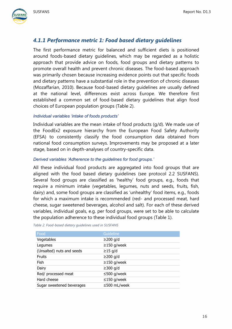
choices of European population groups (Table 2).
Individual variables ‘intake of foods products’
Individual variables are the mean intake of food products (g/d). We made use of
the FoodEx2 exposure hierarchy from the European Food Safety Authority
(EFSA) to consistently classify the food consumption data obtained from
national food consumption surveys. Improvements may be proposed at a later
stage, based on in depth-analyses of country-specific data.
Derived variables ‘Adherence to the guidelines for food groups.’
All these individual food products are aggregated into food groups that are
aligned with the food based dietary guidelines (see protocol 2.2 SUSFANS).
Several food groups are classified as ‘healthy’ food groups, e.g., foods that
require a minimum intake (vegetables, legumes, nuts and seeds, fruits, fish,
dairy) and, some food groups are classified as ‘unhealthy’ food items, e.g., foods
for which a maximum intake is recommended (red- and processed meat, hard
cheese, sugar sweetened beverages, alcohol and salt). For each of these derived
variables, individual goals, e.g. per food groups, were set to be able to calculate
the population adherence to these individual food groups (Table 1).
Table 2. Food-based dietary guidelines used in SUSFANS
Food Guideline
Vegetables ≥200 g/d
Legumes ≥150 g/week
(Unsalted) nuts and seeds ≥15 g/d
Fruits ≥200 g/d
Fish ≥150 g/week
Dairy ≥300 g/d
Red/ processed meat ≤500 g/week
Hard cheese ≤150 g/week
Sugar sweetened beverages ≤500 mL/week
SUSFANS
Report No. D1.3
17
Alcohol ≤10 g/d
Salt ≤6 g/d
Source: Report SUSFANS D2.2 (2016)
The percentage of persons that adhere to these goals is based, not only on the
average consumption within a population, but also on the distribution of that
population. In general adherence to individual guidelines is expected to be low.
We evaluated dietary intakes adjusted to a 2000 kcal per day diet to assess diet
quality independently of diet quantity, and to reduce measurement error within
and across surveys (Willett, 2012).
Performance metric
To derive a performance metric, we constructed a score for the overall dietary
pattern we selected 5 key foods (fruits, vegetables, fish, red- and processed
meat, and sugar sweetened beverages). Intake of foods, rather than
macronutrients or micronutrients, may be most relevant for non-communicable
disease risk (Micha, 2015). Foods and food groups that are mostly included (on
different aggregation levels) in dietary quality indices are fruits, vegetables,
staple foods, sugar, dairy products, and protein sources such as meat, eggs and
plant based proteins (Trijsburg, not published). The Global Burden of Diseases
Nutrition and Diseases Expert Group published their rational to include a
selection of foods related to non-communicable diseases (Micha, 2015). They
included fruit and vegetable intake as these are associated with reduced risks in
CHD, stroke, oesophageal cancer and lung cancer. Fish intake was included
because it reduced the risks of CHD and stroke. Red and processed meat intake
were selected because these are related to increased risk of CHD, diabetes and
colorectal cancer. Sugar sweetened beverages were included due to their
relation with increased risks diabetes and increase in BMI (Micha, 2012). They
also included nuts and seeds and whole grains in their list of key foods.
However, we excluded those as nuts and seeds are often eaten salted, and with
the current assessment method we could not distinguish between salted and
unsalted nuts. Furthermore, we did not include whole grain products as these
are difficult to classify and compare between countries. However, if assessment
methods will improve in the future and can quantify whole grain consumption
better, we advise to include whole grain intake in this diet quality index. For
now, dietary fibre intake, which is highly correlated with whole grain intake will
be included in the nutrient based performance metric. Finally, we did not
include milk as it is highly correlated with calcium intake, which will be included
in the nutrient based performance metric as well.
To derive a summary score for the five key foods, we used previously set cut-
offs for each food item. Capping of intake (defined as food intake is equal to
SUSFANS
Report No. D1.3
18
cut-off value if intake exceeded the cut-off value) will be applied to avoid
crediting of overconsumption (Drewnowski, 2009), and also vice versa for foods
that should be limited. First, the scores will be calculated for each individual.
Subsequently, these individual scores will be averaged to calculated the
population mean. A continuous score between 0 and 10 points will be
calculated based on the average intake of two assessment days. Similar to the
Healthy Eating Index, the five indicators are weighted equally (1/5) in the total
score.
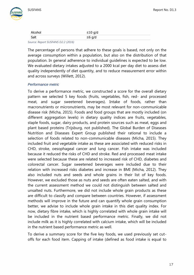
We calculated the scores based on the five indicators (Table 3) with the
following formulas:
If vegetable intake ≥ 200 g then score is 10; if<200 g then score is g vegetable/200*10
If fruit intake ≥ 200 g then score is 10; if<200 g then score is g fruit/200*10
If fish intake ≥ 20 g then score is 10; if<20 g then score is g fish/20*10
If meat intake ≤ 70 g then score is 10; if>70 g then score is 70/g meat*10
If sugar sweetened beverage (SSB) intake ≤ 70 g then score is 10; if>70 g then score is
70/g SSB*10
Table 3. Dietary quality score foods: five selected food items standardised for 2000 kcal/d.
Components Guidelines Healthy diet Maximum
score (=10)
Calculation
score
1. Vegetables Eat at least 200 g/d ≥ 200 g g/200*10
2. Fruit Eat at least 200 g/d ≥ 200 g g/200*10
3 Fish Eat at least 150 g/week ≥ 21.4 g g/21.4*10
4. Red and processed meat Eat at most 500 g/week ≤ 71.4g 71.4/g*10
5. Sugar sweetened
beverages
Drink at most 500
mL/week
≤ 71.4g 71.4/g*10
For example, consumption of 100 g/d of fruits (standardized to 2000 kcal/d) will
give a score of ‘5’ for the component ‘Fruits’. Eating more than the
recommended intake for fruits, vegetable, and fish will not give a higher score.
Each component has a maximum score of 10 points. Scores for each food item
will be summed up and multiplied by 2 to derive at a total score with a
maximum of 100. A score of ‘100’ represents complete adherence to the food-
based dietary guidelines that are included.
This food based performance metric can be used for total populations, e.g.
national surveys, but also for population subgroups. National surveys consist of
individual based data that include also several demographic characteristics.
These can be used to stratify the population according subgroups (age, sex,
BMI, educational level).

SUSFANS
Report No. D1.3
19
4.1.2 Performance metric 2: Nutrient recommendations
The second performance metric for balanced and sufficient diets is positioned
around on nutrient-based recommendations. Food-based dietary guidelines
cover a wide range of foods and thus nutrients, however, some nutrients might
become “of concern”, i.e. are critical nutrients that are not clearly reflected in the
food-based dietary guidelines, and are relevant for public health. Especially,
when shifting from an animal-based dietary pattern towards a more plant-based
dietary pattern some nutrients may not clearly be reflected in the food-based
dietary guidelines.
Individual variables ‘intake of nutrients’
Individual variables are the mean intake (µg/d, mg/d, g/d) of nutrients for which
a minimum intake (protein, vitamins and minerals) is recommended and, mean
intake of nutrients for which a maximum intake should not be exceeded
(saturated fats, added sugars, sodium). Similar to the foods, we will evaluate
nutrient intakes adjusted to a 2000 kcal/d diet.
Derived variables ‘Adherence to the DRVs for individual nutrients.’
For each of the nutrients the percentage of the population that complies with
the dietary recommended values (DRVs) will be calculated, without correction
for within subject variability. DRVs are defined using reference values from
European Food Safety Authority (EFSA, 2010), either average requirement (AR)
or adequate intake (AI) if requirement has not been set, and maximum
recommended values (MRV) using reference values of the World Health
Organisation (WHO, 2003; 2012; 2014). DRVs and MRVs are summarized in
SUSFANS protocol 2.2.
Performance metric
To evaluate European populations’ nutrient intakes, the nutrient density of the
diet was quantified using a Nutrient Rich Diet (NRD) score (van Kernebeek,
2014; Roos 2015) based on the principles of the Nutrient Rich Food Index
(Drewnowski, 2009; Fulgoni, 2009). The NRD algorithm was calculated as:
𝑁𝑅𝐷 𝑋. 𝑌 = ∑𝑁𝑢𝑡𝑟𝑖𝑒𝑛𝑡 𝑖
𝐷𝑅𝑉 𝑖𝑥100 − ∑
𝑁𝑢𝑡𝑟𝑖𝑒𝑛𝑡 𝑗
𝑀𝑅𝑉 𝑗
𝑗=𝑌
𝑗
𝑖=𝑋
𝑖
𝑥100
where X is the number of qualifying nutrients, Y is the number of disqualifying
nutrients, nutrient i or j is the average daily intake of nutrient i or j, DRV is the
Dietary Reference Value of qualifying nutrient i and MRV j is the Maximum
Recommended Value of the nutrient to limit j.

SUSFANS
Report No. D1.3
20
For the present analyses we use the NRD9.3 and the NRD15.3. The NRD9.3
includes nine nutrients to encourage (protein, dietary fibre, calcium, iron,
potassium, magnesium, and vitamin A, C and E) and three nutrients to limit
(saturated fat, added sugar, and sodium) and will be calculated per 2,000 kcal
and capped at 100% DRV. It was primarily chosen based on validation results
among US populations (Drewnowski, 2009; Fulgoni, 2009). To capture more
nutrients that are potentially relevant for EU populations we also used the
extended version, e.g., the NRD15.3 that additionally includes mono-
unsaturated fatty acids, zinc, vitamin D and B-vitamins (B1, B2, B12, folate), but
excluding magnesium.
The NRD9.3 score can range from 0-900 and the NRD15.3 can range from 0-
1500. To rescale it to a range of 0-100 the NRD9.3 and NRD15.3 will be divided
by 9 and 15 respectively. A score of 100 represents complete adherence to the
nutrient recommendations included in the metric.
4.1.3 Performance metric 3: Energy balance
The food and nutrient based performance metric will capture the quality of the
diet including the variety of foods and nutrients consumed. However, because
they are standardized for energy, they do not capture the energy balance. A
measure that reflects the balance between energy intake and energy
expenditure, is the Body mass index (BMI). The percentage of a population
having ‘normal’ weight will be used as a third performance metric. Were 100%
having normal weight is ‘ideal’.
Individual variables
In the national surveys that we use in SUSFANS, we collected additional
information on several population characteristics, including height and weight.
We are thus able to calculated individuals’ BMI and calculated population
averages. We have to note that these data are self-reported and not based on
anthropometric measurements. Usually people tend to underestimate their
weight when it is self-reported. However, these difference are expected to be
relatively small. In the Czech Republic differences between self-reported and
measured normal weight ranged from 7.7-9.6% (Čapková, 2016).
Performance metric
BMI is calculated by dividing an individual's weight (in kilograms) by his or her
height (in meters squared), and is the most common method to quantify weight
across a range of body sizes in adults. Using BMI, individuals can be classified as
normal weight (18.5–24.9 kg/m2), overweight (25–29.9 kg/m2), and obese (>30
kg/m2) (WHO, 1995). It reflects both health and nutritional status and predicts

SUSFANS
Report No. D1.3
21
performance, health, and survival (WHO, 1995). BMI is often used as a proxy for
body fatness in large population studies. Correlations between BMI and more
direct measures of body fatness are generally strong (r>0.70) (Flegal, 2009;
Ranasinghe, 2013; Ablove, 2015; Bradbury 2017).
4.1.4 Extrapolation to EU
We have data available for 4 countries (Czech Republic, Denmark, France and
Italy). These countries represent the different regions in Europe (North, east,
South and West) and account for ~30% of the European population. To
estimate the performance metrics on the EU level we suggest to take the
average of those for countries as they are equally spread across the EU and
represent the North, South, West and East of Europe. When data will become
available for other EU countries (EFSA comprehensive database) we can include
those.

SUSFANS
Report No. D1.3
22
Table 4. Performance metrics for Policy Goal: ‘Balanced and sufficient diet for EU citizens’
Policy Performance metrics Aggregate indicators Derived variable Individual variable
Goal (assessable against targets;
B derived from C)
(C, derived from D) (D, derived from E) Cut-off for D (E)
Balanced and sufficient diet for EU citizens
Food based summary score based on 5 key foods (0-100):
Fruits
Vegetables
Fish
Red & Processed meat intake
Sugar Sweetened Beverages (SSB)
n.a. Vegetables
Legumes
(Unsalted) nuts and seeds
Fruits
Fish
Dairy
Red/ processed meat
Hard cheese
Sugar sweetened beverages
Alcohol
Salt
≥200 g/d ≥150 g/week ≥15 g/d ≥200 g/d ≥150 g/week ≥300 g/d ≤500 g/week ≤150 g/week ≤500 mL/week ≤10 g/d ≤6 g/d
Intake of >1500 food products have been individually assessed in country specific population surveys and have been aligned with FoodEx2 classification system
Nutrient based summary score (0-100)
NRD 9.3
NRD 15.3
n.a. NRD 9.3 includes protein, dietary fibre, calcium, iron, potassium, magnesium, and vitamin A, C and E, saturated fat, added sugar, and sodium. NRD 15.3 additionally includes mono-unsaturated fatty acids, zinc, vitamin D and B-vitamins (B1, B2, B12, folate), but excludes magnesium.
See protocol D2.2 Energy Protein Mono-unsaturated fat Fibre Calcium Iron Magnesium Potassium Selenium Iodine Zinc Vitamin A Vitamin C Vitamin E Vitamin B1
Vitamin B2 Vitamin B6 Vitamin B12 Folate Vitamin D Sodium Saturated fat Total sugar Protein, plant Protein, animal Saturated Fatty Acids (SFA) Mono-Unsaturated Fatty Acids (MUFA) Poly-Unsaturated Fatty Acids (PUFA)
Energy balance % of population with normal weight: 100% is ‘ideal’
BMI (kg/m2): normal weight: 18.5–24.9 overweight: 25–29.9 obese: >30 kg/m2
BMI (body mass index of each country)

SUSFANS
Report No. D1.3
23
4.2 Policy Goal: Reduced environmental impacts of the
EU food system
Our society is facing multiple threats to our environment deteriorating the
quality of the air, the water, the soil, changing our climate, or reducing the
genetic resources or material resources (EEA 2015). The 7th Environment Action
Programme (EAP) of the European Union sets out the vision that “in 2050, we
live well, within the plant’s ecological limits” setting three key objectives4: (i)
protect, conserve, and enhance the Union’s natural capital, (ii) turn the Union
into a resource-efficient, green and competitive low-carbon economy, and (iii)
to safeguard the Union’s citizens from environment-related pressures and risk
to health and wellbeing (EU 2013a). Global climate change is one of the largest
environmental challenges humanity is facing and considerable efforts are
required to limit global warming well below 2.0 or even at 1.5 degree Celsius as
indicated in the Paris Agreement in 2016 (Rogelj et al. 2016). According to
Steffen et al. (2015b), biogeochemical flows of nitrogen (N) and phosphorus (P),
as well as genetic diversity are in the ‘zone’ of high risk, exceeding the planetary
boundaries at global and regional level.
For the SUSFANS project we therefore define four performance metrics with the
aim to achieve:
Climate stabilization
Clean air, soil and water
Biodiversity conservation
Preservation of natural resources
A recent assessment of the impact of agriculture on five main threats (climate,
air, soil and water quality, and biodiversity) concluded that agriculture is a
significant contributor for most of the environmental threats assessed is
dominating some of them, e.g. contributing 55% of air pollutant emissions, 59%
of the N burden of the water systems, and being responsible 51% of loss of
biodiversity in Europe (Leip et al. 2015b). Seafood production causes
considerable pressures on marine ecosystems, of various degree and form in
different areas and from different production systems (e.g. Emeis et al. 2015;
Halpern et al. 2015).
4 See also http://ec.europa.eu/environment/action-programme/

SUSFANS
Report No. D1.3
24
Table 5. Emissions of main pollutants in Europe and share of agricultural sources.
Values are calculated on the basis of the life-cycle (cradle-to-farm gate) approach; emissions from imported
feed are not considered for comparability with estimates for EU27 ter
Total Agricultural
LCA flow within
EU27 territory
Total EU27
budget
flow
Share
agriculture
Air pollution - NH3 emissions
[Tg N yr-1]
2.6 2.7 94%
Air pollution - NOx emissions
[Tg N yr-1]
0.3 2.6 13%
Air pollution - SO2
[Teq yr-1]
0.021 0.35 6%
Air pollution - NOx + NH3 emissions
[Tg N yr-1]
2.9 5.3 55%
Soil acidification
[Tg Teq yr-1]
0.18 0.56 32%
GHG emissions
[Tg CO2eq yr-1]
651 4889 13%
GHG emissions - Carbon sequestration
[Tg CO2eq yr-1]
-93 -170.5 55%
GHG emissions - GHG + Carbon
sequestration
[Tg CO2eq yr-1]
558 4718.4 12%
Water pollution - N
[Tg N yr-1]
5.4 9.1 59%
Water pollution - DIP
[Tg P yr-1]
0.025 0.25 10%
Land Use
[Mio km2]
1.8 4.2 42%
Loss of biodiversity
[relative MSA]
-34% -65% 51%
In the following, we describe the SUSFANS approach to quantify each of the
performance metrics on the basis of suggested aggregate indicators and their
importance for the performance metrics (weighting factor) as well as a possible
vision for the indicators that can be used to benchmark progress towards
reaching the desired goals.
All environmental aggregate indicators should consider the impact from a life
cycle perspective of a supply chains for a food product. This comprises
emissions from agricultural activities (both the cropping and animal sector for
livestock products), but also emissions from agricultural inputs (related to
energy and land use, fertilizers, chemical substances etc.) and emissions from
post-farm gate processes (processing, transport, consumption).

SUSFANS
Report No. D1.3
25
An overview of all metrics for the environment goal can be found in Table 6.
4.2.1 Performance metric 1: Climate stabilization
The societal goal of climate stabilization can be quantified with a single
aggregate indicator measuring the “reduction of total GHG emission caused by
the agri-food chain”.
4.2.1.1 Reduction of total GHG emission caused by the agri-food chain
Description: Total GHG emissions are measured as the global warming
potential of climate relevant gases in CO2-equivalents for a time horizon of 100
years caused by agricultural supply chains. Carbon equivalent emissions are
calculated based on the global warming potentials as defined in the IPCC Fourth
Assessment Report (Ipcc 2007): 𝐺𝑊𝑃𝐶𝐻4 = 25; 𝐺𝑊𝑃𝑁2𝑂 = 298. Even though
more recent global warming potentials are available from the Fifth Assessment
Report (IPCC 2014) (𝐺𝑊𝑃𝐶𝐻4 = 28; 𝐺𝑊𝑃𝑁2𝑂 = 265), those are not yet used in
official national greenhouse gas inventories and results were not comparable
with policy targets or reported emission trends.
Policy vision: A stabilization of the climate at a level well below 2 degree
Celsius above could imply that the current level of greenhouse gases would
need to be reduced thus CO2 re-captured from the atmosphere (Hansen et al.
2008). Possible sinks for CO2 is the land use sector (already today acting as a net
sink in Europe, (EEA 2014)), the agriculture sector (Lal 2016), or technical carbon
capture and storage, potentially related to bioenergy production. Emissions of
CH4 and N2O are natural biogeochemical processes it will be impossible to
completely eliminate those emissions. As it is currently not predictable how
much carbon sequestration in the agriculture sector will be required beyond the
amount required to compensate own GHG emissions, we define thus as policy
vision: zero net emissions from food products supply chains by the year 2100.
Policy targets: Policy targets for the whole EU economy are set in the 2020
climate & energy package (European Union 2015), the 2030 climate and energy
framework (European Commission 2014), and the roadmap for moving to a low
carbon economy in 2050 (European Commission 2011a). These documents
however do not give specific targets for the agriculture sector. However, larger
emission cuts are foreseen for the sectors covered by the EU Emissions Trading
System which should reduce emissions by -43% by 2030, while the so-called
‘non-ETS sectors’ (including road transport, buildings, waste, agriculture and
LULUCF) would need to reduce emissions by -30%, according a proposal5 for
5 https://ec.europa.eu/clima/policies/ets/revision_en

SUSFANS
Report No. D1.3
26
the revision of the ETS and for an Effort Sharing Regulation for emissions in
non-ETS sectors6.
Aggregated variables: The radiative balance of the atmosphere is affected
from both the presence of greenhouse gases in the atmosphere, but also from
reflections of solar radiation on surfaces. Ideally, a comprehensive analysis
would cover two ‘derived variables’ quantifying total CO2-equivalents emissions
caused the supply chain or the agri-food system assessed, and the changes to
the energy balance via land use/cover changes or contributions to changes in
the water balance (Alkama & Cescatti 2016). Greenhouse gases include the main
gases CO2, CH4, and N2O that are emitted from agricultural and energy sources,
but also emissions of climate-forcing cooling agents or other substances that
might be released in the production chain, which can give a substantial
contribution to GHGs of seafood from capture fisheries (Ziegler et al. 2013). In
SUSFANS, only the emissions of greenhouse gases will be considered.
4.2.2 Performance metric 2: Clean air and water
Clean air and water resources are essential for the functioning of ecosystems,
enabling them to provide the services for the benefit of society, and avoiding
health impacts. The benefits derived from ecosystem services cover various
dimensions of human well-being, namely basic human needs, economic needs,
environmental needs and subjective happiness (Maes et al. 2016).
Aggregate indicators considered include therefore the reduction of emissions to
the atmosphere and to the hydrosphere, as well as the reduction of toxic
substances. Main pollutants of relevance in agri-food supply chains are emission
of N and P compounds. A main concern for the quality of drinking is the
presence of nitrates, while a balance between N and P determines the risk of
fresh- and coastal water bodies to eutrophication (Garnier et al. 2010; Leip et al.
2015b).
In SUSFANS, the following aggregate indicators are therefore considered:
Reduction of N surplus
Reduction of N emissions to the atmosphere (air pollution)
Reduction of N emissions to the hydrosphere (water pollution)
Reduction of P surplus
Reduction of Toxic substances use
4.2.2.1 Reduction of N emissions to the atmosphere (air pollution)
Description: Emissions of ammonia (NH3) and nitrogen oxides (NOx) are
impacting air quality with direct health effect, for example through the
6 https://ec.europa.eu/clima/policies/effort/proposal_en

SUSFANS
Report No. D1.3
27
formation of particulate ammonium nitrates, and contributing to multiple
ecosystem damages through deposition. They are precursors of the greenhouse
gas N2O and thus also contributing to global warming. However, in areas with
little nitrogen deposition, additional input of nitrogen through atmospheric
deposition might also lead to an increase of biomass growth (fertilization effect)
(De Vries et al. 2011). Also atmospheric nitrogen compounds might be, ‘filtered’
out with landscape elements protecting more sensitive (semi)natural
ecosystems.
Policy vision: Policy vision is to eliminate emissions of harmful atmospheric
pollutants. If possible the ‘net’ emissions shall be calculated, which means that
recovered nitrogen emissions are subtracted from total emissions and emissions
not contributing to any adverse effect are not accounted for. For the purpose of
SUSFANS, we assume that in Europe nitrogen saturation of ecosystems is
predominant thus all emissions are to be considered. Also, landscape structural
elements for reducing nitrogen pollution are not yet in place and are assumed
to be irrelevant. Therefore, the policy visions translate to zero NH3 and NOx
emissions from agricultural supply chains. In analogy to the policy vision
‘climate stabilization’ we select the target year 2100.
Policy targets: The National Emission Ceilings Directive (NECD) (EC 2001) has
the objective to limit emissions of acidifying and eutrophying pollutants and
ozone precursors in order to improve the protection in the Community of the
environment and human health against risks of adverse effects from
acidification, soil eutrophication and ground-level ozone and to move towards
the long-term objectives of not exceeding critical levels and loads and of
effective protection of all people against recognised health risks from air
pollution by establishing national emission ceilings.
The emission ceilings are defined at the national level, for the agriculture sector
emissions of ammonia (NH3) are most relevant, as more than 90% of NH3
emissions originate from agricultural sources. The directive requires Member
States to draw up a National Programme which includes information on
adopted and envisaged policies and measures and quantified estimates of their
effects on the emissions. Parallel to the development of the EU NEC Directive,
the EU Member States together with Central and Eastern European countries,
the United States and Canada have negotiated the "multi-pollutant" protocol
under the Convention on Long-Range Transboundary Air Pollution (the so-
called Gothenburg protocol, agreed in November 1999). The emission ceilings in
the protocol are equal or less ambitious than those in the NEC Directive.
The NECD was being reviewed as part of The Clean Air Policy Package
(European Commission 2013) and the new National Emissions Ceilings Directive

SUSFANS
Report No. D1.3
28
entered into force in December 2016 (EU 2016) as the main legislative
instrument to achieve the 2030 objectives of the Clean Air Programme. This
Directive sets national reduction commitments for the five pollutants (sulphur
dioxide, nitrogen oxides, volatile organic compounds, ammonia and fine
particulate matter) responsible for acidification, eutrophication and ground-level
ozone pollution which leads to significant negative impacts on human health
and the environment.
Reduction commitments are given for ‘any year from 2020 and 2029’ and for
‘any year from 2030’ compared to the emission level in the year 2005. For EU28,
the targets are -42% and -63% for NOx, and -6% and -19% for NH3. However
national targets vary considerably among countries, for the example of NH3
emission reductions from 2030 onwards, they are between -1% for Estonia and -
30% for Slovakia (EU 2016).
Aggregated variables: Emissions of NH3 and NOx are aggregated to the unit of
total N emissions.
4.2.2.2 Reduction of N emissions to the hydrosphere (water
pollution)
Description: Anthropogenic increase of nitrogen in water poses direct threats
to human and aquatic ecosystems. High nitrate concentrations in drinking water
pose a risk for human health (van Grinsven et al. 2010, 2006). In aquatic
ecosystems the nitrogen enrichment can contribute to eutrophication events,
which are responsible for toxic algal blooms, water anoxia, fish kills and habitat
and biodiversity loss. (Grizzetti et al. 2011). Pressure of nitrogen loads in water
comes from point sources (sewage systems), diffuse sources through leaching
and runoff from agricultural production or diffuse input from (semi)natural
ecosystems. For the year 2002, Leip et al. (2011a) estimate a share of agricultural
sources to be 57%, sewage systems 22%; however the authors include also a
large contribution from nitrogen input through atmospheric deposition on land
or continental shelf regions. As sewage treatment considerably improved during
the last decade, the share of agricultural nitrogen is likely to be higher today.
Contribution to eutrophying emissions from aquaculture mainly comes from the
grow-out site where the species is farmed, even if feed in aquaculture to a large
extent originate from crop production.
Marine Strategy Framework Directive (EU 2008) aims to achieve Good
Environmental Status (GES) of the EU's marine waters by 2020 and to protect
the resource base upon which marine-related economic and social activities
depend. The directive has a special descriptor for eutrophication with the goal
“Human-induced eutrophication is minimised, especially adverse effects thereof,

SUSFANS
Report No. D1.3
29
such as losses in biodiversity, ecosystem degradation, harmful algae blooms and
oxygen deficiency in bottom waters”.
Policy vision: Policy vision is to eliminate emissions of nitrogen emissions to
the hydrosphere. If possible the ‘net‘ emissions shall be calculated, which means
that recovered nitrogen emissions are subtracted from total emissions and
emissions not contributing to any adverse effect are not accounted for. Even
though buffer zones and artificial wetlands are already used for the restoration
of water courses, no suitable data is available allowing the quantification of the
magnitude of their impact. Therefore, for the purpose of SUSFANS, we use zero
nitrogen leaching and run-off as the policy vision. Again, in analogy to the
policy vision ‘climate stabilization‘ we select the target year 2100.
Policy targets: The Nitrates Directive (EC 1991) forms an integral part of the
Water Framework Directive (EU 2000) and is one of the key instruments in the
protection of waters against agricultural pressures. It has the objective reducing
water pollution caused or induced by nitrates from agricultural sources and
preventing further such pollution. The directive requires the Member State to
monitor nitrate concentrations in surface water and groundwater, identify
waters affected by pollution and waters that could be affected by pollution if no
measures are taken and designate vulnerable zones where action programmes
containing measures to reduce and prevent nitrate pollution must be
developed, implemented and revised every four years. The corner stones of the
directives are (i) the designation of vulnerable zones; (ii) the establishment of a
Code of Good Agricultural Practice, and (iii) the implementation of Action
Programmes describing required measures. Such Action Programmes can vary
regionally depending on local conditions and pollution levels. The only pre-
scribed quantitative measure given in Annex III of the ND is the limit of applied
livestock manure of 170 kg ha-1 yr-1. However, some countries have asked
derogation. Currently there are eight derogations in force. As such, it is difficult
to formulate a concrete policy target for the reduction of emissions of nitrogen
to water. Furthermore,
There is a strong regional variability in the effect of nitrogen emissions to water, also reflected in
the designation of ‘nitrate vulnerable zones’
The nitrates directive focuses on the impact of nitrates on drinking water, while other effects
linked other effects such as eutrophication of coastal zones are regulated in regional policies, such
as the OSPAR convention, where 15 Governments and the EU cooperate to protect the marine
environment of the North-East Atlantic.7
In 2015, the EU court of justice ruled in a case (“Weser case”) that a country
must refuse authorisation for projects that may cause deterioration of the status
7 http://www.ospar.org/about

SUSFANS
Report No. D1.3
30
of a water body, unless derogation is granted. Deterioration of the status is
given as soon as one quality element (Annex V of the directive) falls by at least
one class.8
For SUSFANS, we therefore suggest use the linear interpolation of the emission
level in the reference year and zero emissions by 2030 to the policy target year.
Aggregated variables: Emissions of nitrates and organic nitrogen to the water
are aggregated to the unit of total N emissions.
4.2.2.3 Reduction of N surplus
Description: The Gross nitrogen balance (or nitrogen surplus) is regarded as key
indicator in many agri-environmental frameworks aiming at monitoring the
effectiveness of agricultural and environmental policies. The Gross nitrogen
balance is calculated from total N in manure excreted by animals and/or
imported to a farm and other inputs such as biological nitrogen fixation,
atmospheric deposition and other applied fertilizers, and N in outputs (crop and
livestock products) (Eurostat 2013; Leip et al. 2011b). The N surplus therefore
includes all losses to the environment (atmosphere and hydrosphere) from
livestock and crop production systems.
Despite this ‘overlapping’ with the aggregate indicators ‘Reduction of N
emissions to the atmosphere’ and ‘Reduction of N emissions to the
hydrosphere’, the aggregate indicator ‘Reduction of N surplus’ is still important
because N surplus is a very common indicator; it includes losses of N2, which are
not included in the other aggregate indicators and are relevant for resource use
efficiency (Pelletier & Leip 2013). Closing of the nitrogen cycle – that is
reduction of the need for new nitrogen fixation is seen also as one big challenge
for the global planetary boundaries (Rockström et al. 2009; Steffen et al. 2015a)
The monitoring of Nitrogen balances is required for each Member State’s RDP
2007-2013 as part of the EU’s Common Monitoring and Evaluation Framework
(CMEF, EU 2013b). The monitoring of Nutrient balances is relevant also in other
policy domains such as: the Water Framework Directive (EU 2000) requiring
Member States to protect and restore the quality of their waters; and the
Nitrates Directive (EC 1991), aiming to reduce water pollution caused or induced
by nitrates from agricultural sources and prevent further such pollution.
In contrast to the other aggregate indicators, the N surplus is calculated per
area of utilized agricultural land required for the production of a food product
(including land for feed) and represents thus not the total absolute emissions in
8 http://curia.europa.eu/juris/document/document.jsf?text=&docid=165446&pageIndex=0&
doclang=EN&mode=req&dir=&occ=first&part=1&cid=9592

SUSFANS
Report No. D1.3
31
kg N yr-1 cause by the food chain, but the average losses of nitrogen to the
environment per hectare of land used [kg N ha-1 yr-1].
Policy vision: Due to the overlapping of the N surplus with emissions of
nitrogen to atmosphere and water, no separate policy goal vision to be
formulated. The N surplus has no influence on the performance metrics ‘clean
air and water’ (weight=0) as it is already covered by the mentioned aggregate
indictors.
Policy targets: not applicable.
Aggregated variables: Balance of total N inputs and total N outputs: Inputs:
mineral fertilizer, manure imported to the farm or excreted by animals, other
organic fertilizers applied, atmospheric deposition, biological nitrogen fixation.
Outputs: N in crop products harvested and livestock biomass and livestock
products sold.
4.2.2.4 Reduction of P surplus
Description: Phosphorus and phosphates contribute to aquatic (freshwater and
marine) eutrophication and to coastal water eutrophication by providing
limiting nutrients to algae and aquatic vegetation in excess of natural rates,
leading to an alteration of aquatic species composition and productivity
(Henderson 2015). Leip et al. (2015b, see Supplementary Information S4)
assessed the limiting factor for a total of 24 European watersheds with the
GREEN model (Grizzetti et al. 2012) on the basis of the ICEP approach (Garnier et
al. 2010) and found most watersheds being P rather than N limited. Emissions of
P to the atmosphere are usually considered negligible and occur mainly via wind
erosion processes. Therefore, the P surplus aggregated indicator can be used for
describing P losses to the aquatic system. P is less mobile in soils than N and
might be ‘sorbed’ to soil minerals and thus become unavailable to plant uptake,
but also not being at risk of contributing to water eutrophication (Redding et al.
2016). However, in contrast to N, P is a scarce resource, which needs to be
‘refilled’ from natural deposits if it is dispersed in to the environment. In
SUSFANS, this ‘resource’ dimension is integrated into the aggregate indicator
‘reduction of P surplus’ which is therefore measured as the input of ‘new’ P to
the food supply chain as mineral fertilizer, while recycled sources of P (in
manure, compost, sewage sludge etc.) are not included.
Policy vision: Policy vision is a full recovery of P into the agro food system with
zero P surplus and thus zero addition of new P. We select the target year 2100
in analogy to the climate stabilization aggregate indicator.

SUSFANS
Report No. D1.3
32
Policy targets: In the absence of quantified policy target for mineral P fertilizers,
we use the linear interpolation of the emission level in the reference year and
zero emissions by 2100 to the policy target year.
Aggregated variables: P application in mineral fertilizers.
4.2.2.5 Reduction of Toxic substances use
Description: Toxic substances, heavy metals and pesticides and other plant
protection chemical substances and substances given to livestock pose a threat
to organisms in the environment. Some substances are regulated, other are
permitted to be use because sufficient evidence for the adverse effect has not
been found, or because the benefit of the substances is believed to outweigh
their risk. In SUSFANS we focus on pesticides and plant protection chemicals for
which data are available in the models.
Policy vision: We set the policy vision is zero application of harmful substances
by 2030. Ideally this takes into consideration the different levels of toxicity of
different chemical agents if this information is available.
Policy targets: In the absence of quantified policy targets for the application of
toxic substances, we use the linear interpolation of the emission level in the
reference year and zero emissions by 2030 to the policy target year.
Aggregated variables: The aggregate indicator is derived from the individual
variable on the usage of substances in the scope of plant protection and crop
growth regulatory measures. In SUSFANS, no differentiation is made between
different chemical products, as information on efficiency and harmfulness of the
different agents used is not available. Therefore, all application of herbicides,
fungicides, insecticides, as well as growth regulatory measures are considered.
Aggregation is done based on a monetary value obtained e.g. from the
Economic Accounts of Agriculture provided by Eurostat. The data is the sum of
expenditures for all non-mechanical plant protection measures and is corrected
by the inflation rate to account for price changes between the reference and the
target year.
4.2.3. Performance metric 3: Biodiversity conservation
Food supply chains might affect biodiversity both directly through reduction of
farmland biodiversity and marine biological diversity, and indirectly through
land use change, land fragmentation, and pollution processes; pressures are
often larger outside of the EU than within, masked by international supply
chains (Lenzen et al. 2012). In SUSFANS, we assess biodiversity conservation
with three indicators focusing on general terrestrial (non-farmland) biodiversity,
farmland biodiversity, and marine biodiversity.

SUSFANS
Report No. D1.3
33
4.2.3.1 Reduction of the contribution of the agrifood chain to loss of Mean Species Abundance (MSA)
Description: Terrestrial biodiversity is affected through land use and pollution
effects. Land use effects include (historic) land use changes, land fragmentation
with consequently truncation of migratory routes (Reid et al. 2010). Pollution
effect can be direct through deposition of nutrients affecting soil acidity and
(micro)organism composition (Dise et al. 2011; Stevens et al. 2010), or indirectly
via climate change (Alkemade et al. 2009).
The Mean Species Abundance (MSA) represents an index of the naturalness of
an ecosystem. This indicator has been linked to causes of loss of species
abundance in the GLOBIO-model (Alkemade et al. 2009; Kram & Stehfest 2012;
van Vuuren et al. 2015) and attributes 64% of MSA loss to land conversions,
30% to land fragmentation and 5% to pressures from atmospheric deposition
and climate change (Leip et al. 2015b).
Land use is therefore the single most important indicator for terrestrial
biodiversity. It is measured in total area required for the food supply chain. It
should be calculated on the basis of an LCA thus considering also land use
embedded in imported (feed) products, multiplied with the total consumption
of products. This aggregate indicator, however, is of importance beyond the
relevance for biodiversity: low land requirements for agricultural production
alleviates the pressure on land and reduces land competition. For example,
according to current scenarios for the targets of 2 or 1.5 degree, afforestation
and biomass production is needed, and the necessary area could go to 800 Mha
by 2100 or higher (Popp et al. 2017); agriculture will need to contribute to
making this possible.
Policy vision: No further increase for land used for agricultural production. In
contrast to most of the other aggregated indicators, this is an absolute policy
vision which needs to consider the number of persons.
Policy targets: Same as policy goal.
Aggregated variables: Land use [ha]
4.2.3.2 Agricultural land use diversity
Description: Agricultural land use diversity could be approximated by the
concept of ‘Biodiversity-Friendly Farming Practices’ (BFP) which captures the
causality between certain types of farming activity and their potential impacts
on biodiversity. This is closely linked to the High Nature Value (HNV) farmland
and is therefore a key indicator for the assessment of the impact of policy
interventions with respect to the preservation and enhancement of biodiversity,
habitats and ecosystems dependent on agriculture and of traditional rural

SUSFANS
Report No. D1.3
34
landscapes. Terres et al. (2012) define BFP as a composite indicator with four
sub-indicators (arable crops: Shannon index and N input index, grassland:
stocking density index, permanent crops: N input, olive groves: surface).
The BFP indicator is calculated at high spatial resolution, such as the
disaggregated results from the CAPRI model (Leip et al. 2015a).
In order to avoid duplication with other aggregate indicators, we use the
Shannon index as proxy for agricultural land use ‘patchiness’ (Weissteiner et al.
2016) or diversity in SUSFANS. In contrast to most aggregate indicators,
agricultural land use diversity cannot be calculated for individual food supply
chains, as it intrinsically evaluates local crop diversity of agricultural systems. The
aggregate indicator is therefore calculated as the average Shannon index of the
farms/spatial units which contribute to the food supply chain.
Policy vision: A policy vision for agricultural diversity is difficult to define. The
vision formulated in the states EU biodiversity strategy (European Commission
2011b) “By 2050, European Union biodiversity and the ecosystem services it
provides — its natural capital — are protected, valued and appropriately
restored for biodiversity's intrinsic value and for their essential contribution to
human wellbeing and economic prosperity, and so that catastrophic changes
caused by the loss of biodiversity are avoided.”. We here tentatively set a goal of
an increase of the Shannon index by two points until the year 2050. Note that
this is a relative measure and interpretation might vary depending on the
implementation of the Shannon index in different models. Possible, regional
differentiated policy visions might be defined, taking protected areas and
species hotspots into consideration.
Policy targets: Linear interpolation of the Shannon index calculated for the
reference year and the value plus two points by 2050 to the policy target year.
Aggregated variables: The Shannon’s entropy index 𝐻𝑟 is a measure for the
crop diversity in a region r, which is one of the ‘greening’ elements that had
been introduced in the latest CAP reform (EU 2013c). The index is computed
based on the agricultural sector’s land use variety, i.e. the higher the number i of
different crops 𝑝𝑖 including grass cultivated and the more homogeneous their
distribution (thus less dominance from few crops), the higher the diversity:
𝐻𝑟 = − ∑ 𝑝𝑖𝑙𝑛𝑝𝑖
𝑁
𝑖=1
𝐻𝑟 increases with the number of different land use types 𝑁 and if their shares in
the total agricultural area 𝑝𝑖 are more equal. The index is zero if there is only
one land use type 𝑝𝑖 in the sector. In the CAP, crop diversity has to be evaluated

SUSFANS
Report No. D1.3
35
at farm level, which is not possible with the models available in the SUSFANS
toolbox. An evaluation at regional or country level is not meaningful, as the
aggregation from farm to larger areas introduced an aggregation bias and
disconnects the Shannon index from local crop diversity which is used as proxy
for local biodiversity. In the CAPRI model, the Shannon index can be calculated
on the basis of FADN single farm data using the CAPRI farm layer (see Leip et al.
2015a) or on the basis of homogeneous spatial units at the level of 1km x 1km
pixels using the CAPRI spatial layer.
4.2.3.3 Marine biological diversity
Description: Seafood from capture fisheries represents the only large-scale
food production based on a wild resource. It is sometimes argued that fisheries
is be a good alternative to produce food with less impacts and resource use
than many land-based protein production systems, as fisheries do not require
inputs like feeds, fertilizers or pesticides. However, there are limits to natural
production, and many stocks are overexploited and thus produce less than
optimal. Direct and indirect ecosystem effects from over-exploitation include
feedback such as altered ecosystem functioning (Howarth et al. 2014). This is
manifested in the form of depletion of predatory fish (Christensen et al. 2003),
collapse of major fish stocks (Pinsky et al. 2011), altered seafloor structure and
function (Tillin et al. 2006) and biodiversity loss of target and non-target species
(Dulvy et al. 2003; LEWISON et al. 2004). From an ecosystem production
perspective, it has been estimated that current global fisheries exceed levels of
sustainable exploitation, and have to decrease considerably to avoid risk of
impaired function (Coll et al. 2008; Watson et al. 2015); the full effects of
fisheries on marine ecosystems are still largely unknown.
Environmental pressures from aquaculture include: some species and farming
practices require high level of feed input based on capture fisheries and may
release invasive species, cause eutrophication, conversion of ecologically
sensitive coastal land, and transmit diseases to wild fish (Diana 2009).
Policy vision: The vision of the descriptor on marine biodiversity in the Marine
Strategy Framework Directive (EU 2008) states that the “quality and occurrence
of habitats and the distribution and abundance of species are in line with
prevailing physiographic, geographic and climatic conditions.” There are also
several other commitments, agreements and policies of relevance to the EU
goals on marine biodiversity, to mention a few:
The Convention on Biological Diversity (1992) is a multilateral treaty with
commitments to conserve and sustainable use of biological diversity in order to halt
rate of biodiversity loss. One proposed indicator is the Red List Index (RLI; Butchart

SUSFANS
Report No. D1.3
36
et al. 2010, 2005), measuring the trend in proportion of threatened species occurring
(species complexes or nationally).
Agreement on the Conservation of Small Cetaceans of the Baltic, North East Atlantic,
Irish and North Seas (ASCOBANS), with the goal to protect marine mammals.
The Birds Directive, protecting birds.
The Habitats Directive, requires e.g. establishments of Special Areas of Conservation
(target amounts) including marine habitats.
We set the SUSFANS policy vision to no adverse effects on marine habitats and
non-commercial marine species from seafood production from either capture
fisheries or aquaculture.
Policy targets: The descriptor for marine biodiversity in the Marine Strategy
Framework Directive should be a good, overarching target for the SUSFANS
policy vision. However, there are different national indicators to measure
progress towards achieving Good Environmental Status of EU coastal waters by
2020, and many are not developed yet. Therefore, this cannot be included at
this point.
Aggregated variables: Not applicable.
4.2.4 Performance metric 4: Preservation of Natural Resources
4.2.4.1 Sustainable water use
Description: Freshwater is regarded as one of the most important resources of
the planet with agriculture being one of the largest consumers, with a current
estimate of four billion people facing water scarcity today (Mekonnen &
Hoekstra 2016). Climate change is likely to aggravate water scarcity and increase
the number of people living with less than 500 m3 of water per capita and year
available (Schewe et al. 2014). Assessing sustainable use of water poses a
particular challenge because of its large regional, but also temporal variability in
water stress (Pfister & Bayer 2014) and the global water flows embedded in
traded products (Vanham & Bidoglio 2014). The water footprint concept
comprises the ‘blue’, ‘green’ and ‘grey’ water footprints, whereby the blue and
green water footprints are associated with water consumption while the grey
water footprint deals with water pollution (Hoekstra et al. 2011), whereby the
green water footprints accounts for rain-fed water consumption and the blue
water footprint for water evapotranspiration from additional irrigation water
(Mekonnen & Hoekstra 2011).
Water use efficiency needs to increase substantially which is reflected in
Sustainability Development Goals “Ensure availability and sustainable
management of water and sanitation for all “9, in particular target 6.4 (increase
9 https://sustainabledevelopment.un.org/sdg6

SUSFANS
Report No. D1.3
37
water use efficiency) and here indicator 6.4.2 “Level of water stress: freshwater
withdrawal as a proportion of available freshwater resources”
According to indicator 6.4.2, water stress is the ratio of water use (withdrawal)
and water availability. Various authors point out that environmental flows that
are required to maintain ecosystem services functioning need to be included
(e.g. Mekonnen & Hoekstra 2016; Vanham et al. 2009). Also, return flows should
be considered, thus using net rather than gross water abstraction (Mekonnen &
Hoekstra 2016).
As many data required for a detailed assessment are not available for SUSFANS,
we measures sustainable water as water consumption of blue and green water.
Policy vision: In theory, a zero blue water footprint is possible (Vanham &
Bidoglio 2013); for the blue water footprint, we use a policy vision of zero blue
water consumption in a food supply chain, recognizing however that zero blue
water use is not realistic for some parts of Europe and also not required,
depending on the renewal rate of blue water. However, also green water
consumption might pose an environmental problem depending on the its
impact on the local water stress and water environmental flows (Vanham &
Bidoglio 2013). We therefore tentatively set a policy vision of a reduced green
water footprint of 20% below reference situation. In accordance to the SDG
target year, we set the target year for the policy goal to be 2030.
Policy targets: Linear interpolation to the policy target year as policy target,
calculated from the water use calculated for the reference year and the value
plus two points by 2030, or policy goal if the policy target year is 2030 or late.
Aggregated variables: Green and blue water consumption. If possible, they
should be calculated separately, and their progress towards the policy goal
averaged.
4.2.4.2. Sustainable exploitation of wild-caught seafood resources
Description: Capture fisheries have been proven to be challenging to manage.
Research on how to define sustainable production levels has been intensive.
One concept is the Maximum Sustainable Yield MSY (Mace 2001), the current
management objective for yield in EU fisheries (EU 2014). Maximum Economic
Yield MEY instead of MSY may allow for more profitable fisheries with a
“biological buffer” (Marchal et al. 2016).
Today around 2500 species (or groups of species) are fished for, based on FAO
landing statistics. Since the late 1980s, global production of capture fisheries has
remained relatively constant; the limit has been reached. According to the latest
estimates (2013), roughly 31% of the stocks were fished at unsustainable

SUSFANS
Report No. D1.3
38
exploitation levels; 58% were fully fished whereas 11% under-utilized (FAO
2016)
Policy vision: The Common Fisheries Policy has set the target that stocks
should be fished allowing for maximum Sustainable Yield (MSY) by 2020.
Policy targets: Distance to optimum exploitation F/FMSY (see aggregated
variables). Progress in this objective has been made in the northern fishing
areas, while the Mediterranean shows little success (EU 2014).
Aggregated variables: Fishing pressure F and optimum fishing pressure FMSY
These values vary between stocks and years and are not yet available for all
stocks exploited in the EU. They are reported on an annual basis by the
International Council for the Exploration of the Seas (ICES) for stocks in the
Northeast Atlantic.
4.2.4.3. Maintenance of soil fertility
Description: Soil quality is influenced by a large number of factors, including
soil acidification, mainly through deposition of N compounds, level of organic
matter (linked to the GHG balance), soil physical quality (e.g avoiding
compaction and/or soil erosion). Several of these threats to soil quality are
already covered in other aggregated indictors.
In SUSFANS we therefore assess the aggregate indicator ‘maintenance of soil
fertility’ by defining soil degradation in terms of loss of soils by soil erosion.
Policy vision: Long term policy vision is an increase of soil organic matter in
agricultural soils. At the climate change negotiations at the 21st Conference of
the Parties to the United Nations (UN) Framework Convention on Climate
Change (COP21) in Paris (November 30 to December 11, 2015), the “4 per
Thousand” proposal was launched calling for a voluntary action plan to enhance
soil organic carbon (SOC) content of world soils to a 40 cm (16 in) depth at the
rate of 0.4% per year (Lal 2016; UNFCCC 2015).
Policy targets: In line with policy vision.
Aggregated variables: Loss of soil with soil erosion.

SUSFANS Report No. D1.3
39
Table 6. Performance metrics for Policy Goal: ‘Reduction of environmental impacts’
Policy goals
Performance metrics
(assessable against
targets; B derived
from C)
Aggregate indicators
(C, derived from D)
Derived variable
(D, derived from E)
Individual variable
(E)
Reduction of
Environmental
impacts
Climate stabilization Reduction of total GHG emissions
caused by the agri-food chain
CO2 eq. CO2, CH4, N2O (Emissions according to IPCC categories incl.
indirect land use change, per unit of product in food consumed
(LCA) = C footprints)
Use/emissions of cooling agents in fish production (CFCs)
Radiative Forcing Land Cover (e.g. albedo)
Clean air and water Reduction of N surplus Nitrogen surplus N input (fertiliser, manure, atmospheric deposition, biological
fixation, feed) and N output (yield), change of soil stocks. Maybe
split of N surplus into emissions to the atmosphere: air pollution
and emissions to the hydrosphere: water pollution)
Reduction of N emissions to the
atmosphere (air pollution)
Emissions of Nr to the atmosphere
(NH3, NOx)
Emissions of NH3, NOx
Reduction of N emissions to the
hydrosphere (water pollution)
Emissions of Nr to the hydrosphere
(Nitrates, Organic N)
Emissions of NH3, NOx
Emissions of NO3, other run-off, leaching
Reduction of P surplus Phosphorus surplus P input and output
Reduction of Toxic substances use Toxic substances use Use of toxic substances (pesticides, …)
Biodiversity
conservation
Reduction of the contribution of
the agri-food chain to loss of
Mean Species Abundance (MSA)
Contribution to loss of Mean
Species Abundance (MSA)
calculated with the GLOBIO model
(Alkemade et al., 2009)
Land use
Emissions of GHGs, Nr
Land use Land use (Shannon) The Shannon’s entropy index (Hr)
seafloor area impacted (m2)
Protected areas (GLOBIOM) Land use map
Species rich hotspots (GLOBIOM) Land use map
Reduction in number of
threatened species
Red List Index (RLI) IUCN Red List threat status (terrestrial and marine) of affected
species
Preservation of
natural resources
Sustainable water use [e.g.
maintenance of environmental
flows]
Terrestrial water scarcity footprint Irrigation water use
Water use in livestock production
Water use in the food chain
Water supply
Sustainable exploitation of wild- distance to optimum exploitation Fishing mortality (F)

SUSFANS Report No. D1.3
40
caught seafood resources (F/FMSY)
%PPR relative to total available
ecosystem production
primary production required (PPR)
Maintenance of soil fertility Soil degradation Erosion
Soil carbon contents

SUSFANS
Report No. D1.3
41
4.3 Policy goal: Competitiveness of EU agri-food
businesses
This section aims at clarifying the comparative concept of competitiveness and
at presenting the metrics to assess the competitiveness within the framework of
the SUSFANS project. To that end, we:
1. Discuss the concept of competitiveness and present a definition of this concept that
will be used in this study (Section 2).
2. Present an overview of competitiveness metrics. These metrics are derived from two
perspectives: the competition on markets for the final product and the competition
for inputs enabling production. The metrics are based on trade and production
performances (Section 3).
3. Present the metrics from individual variables to the performance metrics for the
spider diagram (Sections 3 and 4)
4. Discuss some issues, including the selection of countries and EU member states, the
coverage in terms of sectors and industries, and the pertinent selection of deflators
for the selected sectors and the overall economic activities for each country (Section
5).
We will not address the linkages between competitiveness and policies and we
will not test the relation between competitiveness and performance on
sustainable food security or economic issues.
All data can directly be derived from the GTAP model. These data are in
monetary values and no quantities are available. All indicators will be based on
the outcome of GTAP and always derived from values.
As for the terminology, we use the approach developed by the SUSFANS team:
E: Individual variable that is directly available from a database or a result of GTAP
model.
D: Derived variable that is based on one or more individual variables. In the
sections below, we add a number to these variables. For instance, D1 as first
derived variable, D2 as second and so on.
C: Aggregate variable that evaluates a derived variable. This variable will be
indicated with C and the number of the derived variable: e.g. C1 which will be
linked to derived variable D1 and so on. However not all derived variables will
be also an aggregate variable at C level. We will mention these few exceptions
in the text and these are not included in the summary overview.
B: The performance indicator based on an aggregate variable.
A: Overall performance metrics that includes all performance indicators.
An overview of all metrics for the competitiveness goal can be found in Table 8.

SUSFANS
Report No. D1.3
42
4.3.1 Competitiveness: comparative and multidimensional
Competitiveness is often used in policy statements. The European Council
expressed in 2000 the strategic goal that European Union has set for the next
decade: “...to become the most competitive and dynamic knowledge-based
economy in the world...” (European Council 2000). The Council assumes that a
“competitive economy” contributes to a sustainable economic growth and more
employment. However, in 1994 Krugman stated that from an empirical point of
view the contribution of competitiveness to economic performance and policies
is almost completely unfounded (Krugman 1994). The concept of
competitiveness is complex as the following statement by Spence and Hazard
(1998) illustrates it:
“The problem of international competitiveness has been defined in highly diverse
ways. These definitions (and the proposed solutions to the problem) are partially
inconsistent, and thoroughly confusing to most academics, politicians, policy-
makers, and business managers. There is good reason for this confusion. The
collection of problems alluded to, as “competitiveness” is genuinely complex.
Disagreements frequently occur not only at the level of empirical effects and of
policies, but also in the very definition of the problem.” (Spence and Hazard
1998).
In this section, we will discuss elements of the concept competitiveness or
aspects that are related to it. In next section, we will elucidate the indicators
generally used for measuring competitiveness and the empirical background in
order to minimize the confusion that might occur. Several authors (Buckley, Pass
et al. 1988, Durand, Simon et al. 1992, Metcalfe, Georghiou et al. 1992, Krugman
1994, Crouch and Ritchie 1999, Latruffe 2010, Gorton, Hubbard et al. 2013,
Siudek and Zawojska 2014) presented definitions of competitiveness and
discussed the concepts and indicators.
Based on these papers, we can conclude that competitiveness is a comparative
concept; it has different aggregation levels, is often multi-dimensional, it can be
assessed by different theories, is defined in diverse ways for different time
horizons. Furthermore, competition has two sides: selling your products or
acquiring inputs. In other words, competition means on the one hand acquiring
market shares for your final products and on the other hand to be able to buy
means of production. Below these key words are discussed.
Comparative concept: Latruffe (2010, p50) states that ‘competitiveness
should be measured with respect to a benchmark.’ Competitiveness is a
comparison between entities, e.g. firms or industries in different countries
(Siggel 2006). The outcome depends on who is compared with whom and will

SUSFANS
Report No. D1.3
43
accordingly differ with the selection of entities. Being successful in
competition with one specific entity, does not mean that you are also
successful in the competition with other entities. In this study, the outcome of
the metrics fully depends on the selection of countries. In contrast to several
other aspects of the SUSFANS approach, no fixed policy target can be
defined for competitiveness. For that reason, a fixed selection of countries/or
regions has to be defined and the performance metrics will be dependent on
the outcome of the measurements of the selected countries. The level of the
measure compared to benchmark countries indicates the level of
competitiveness. Hence we compare the measures of country i with
benchmark countries. The next example clarifies this point. The indicator is
the world market share of country i, the competitiveness measure the growth
of the export world market share of country i (difference of market share in
period 2 compared to period 1). A growth of this measure as such is by
definition not always strong. It will be indicated as strong if the benchmark
countries have a lower growth or a decline. However, if the benchmark
countries have a higher growth in market share than country i, the indicator
will be valued as weak.
Aggregation level: Competitiveness is measured for ‘goods or services,
people, firms or countries’ ((Buckley, Pass et al. 1988), p177). In the economic
literature also industries are often mentioned as competing entities (Latruffe
2010). E.g., the five competitive forces of Porter determine industry
competition (Porter, 1990, p35). This study analyses the competitiveness of
the EU food system or in our wording at industry level in a country/union.
The food system can be disaggregated into several sub-industries. The
GTAP/Magnet Model offers the opportunity to distinguish several subsectors
e.g. food and drinks as total, dairy processing, meat processing or primary
producers. Recognizing different groups of players along the value-chain
enables analyses of the impact for these groups. Success of one industry can
indeed go at the cost of an industry down- or up-streams within a country.
For example, the successful industry might be able to negotiate low prices for
the inputs which make the supplying industry less successful (Metcalfe,
Georghiou et al. 1992).
Multi-dimensional: Several authors stress that competitiveness cannot be
defined by a singly indicator (Metcalfe, Georghiou et al. 1992, Sagheer, Yadav
et al. 2009). Porter argues that in any industry five forces determine the long
run competition, whether international or domestic, of an industry10. Each
10
Namely: the threat of new entrants, the bargaining power of buyers, the bargaining power of
suppliers, the threat of substitute products or services and the rivalry among existing firms.

SUSFANS
Report No. D1.3
44
force is built on several indicators (Porter 1980). Porter’s diamond-shaped
model for analysing competition between nation distinguishes four
determinants, each of them also characterised by several sub-determinants
for determining the competitiveness between nations (Porter 1990). Buckley
et al. propose also several indicators, depending on the (aggregation) level of
analysis and time horizon (Buckley, Pass et al. 1988). The World Economic
Forum, for instance, distinguishes over 100 indicators divided in 12 pillars to
access the global competitiveness of countries (Schwab 2014). Several
indicators of the World Economic Forum can be indicated as institutional
factors e.g. infrastructure or policies of the government. Siggel as well as
Latruffe underline this need to include not only economic (costs, productivity,
value added) and trade indicators (unit values, export indicators) but also
institutional factors (Siggel 2006, Latruffe 2010). In our approach of the
competitiveness, we will focus on economic and trade indicators. The other
elements are addressed under different headings in other parts of the
SUSFANS study. Furthermore, the dimensions for the analysis of
competitiveness depend on the aim of the study. Krugman e.g. argues that it
makes little sense to measure the competitiveness on the export market if the
industry is (almost) fully focused on the domestic market (Krugman 1994). For
that reason, we will include not only trade indicators but also indicators
reflecting the domestic production performance and the importance of the
domestic market.
Theoretical foundation: Several theories or schools of thought aim at
defining and analysing competitiveness (Siggel 2006, Latruffe 2010, Jambor
and Babu 2016) resulting in a large number of definitions. From a strategic
management perspective, competitiveness refers to the conduct of
companies in shaping organisational advantages (Wright, Kroll et al. 1998,
Thompson and Strickland 2003) and/or market advantages (Hamel and
Prahalad 1994). Financial ratios (e.g. profit margin, current ratio, return on
assets, debtor and collector period) are the metrics often used in accounting
(Fleisher and Bensoussan 2003, Drury 2013). Measuring competitiveness with
international economic indicators has its roots in Adam Smith’s trade theory,
which explains differences in competitiveness by way of absolute cost
differences between countries. However, the application of new trade
theories entails incorporating a wider array of aspects in the analysis such as
product differentiation, innovation, economies of scale and productivity (Van
Berkum and Van Meijl, 2000). O’Mahoney and Van Ark focus on productivity.
In their study, productivity differences explain largely differences in
competitiveness (O'Mahoney and van#Ark 2003). These are some examples
of the impact of different theories on the metrics of measuring

SUSFANS
Report No. D1.3
45
competitiveness. In this study, international economics will be used in
deriving the metrics for competitiveness
Time horizon: Several authors use sustainable gain in e.g. market share:
hence a comparison between two periods and time horizons play a role
(Siggel 2006). According to Porter (1980, 1990), sustainable competitive
advantage is the fundamental source for above-average performance in the
end. Buckley et al. (1992) introduce the dynamic aspect in the measurement
of competitiveness based on three characteristics: competitive performance,
potential and process, each with different indicators.
Inputs: Being competitive means that the sector is able to source sufficient
resources like labour, capital or raw materials. This means competition for
inputs with other sectors. These two angles of focus – competition on
markets for final products and on markets for inputs- are derived from the
concept of comparative advantage. Comparative advantage has two
dimensions:
Cost of uniqueness of the advantage. This requires a comparison
between domestic and foreign sectors or products on a specific final
market. Indicators related to the final product and the benchmark
measure this concept.
Efficiency gap. Even if a sector performs well, other sectors might perform
even better. For instance, the food sector of one country is the highest
performer compared to the benchmark countries. However, on national
level other sector might perform even better. In the long run, the sector
that is thought to be successful performs less well than such partial
competitiveness studies predict because other sectors in that specific
country outperform this internationally high performing food sector (Van
Berkum and Van Meijl, 2000). This is the competition for production
factors: Is the performance of the sector compared to other sectors
sufficient to compete successfully for means of production? Wijnands et
al. make a comparison of the development of the value added with
another sector (Wijnands and Verhoog 2016). Other measure could be
labour productivity or total factor productivity (O'Mahoney and van Ark
2003).
Based on these considerations we use the following working definitions:
‘Competitiveness is the ex-post performance of a sustained ability to achieve
gains in value added, productivity, employment or world export market share’.

SUSFANS
Report No. D1.3
46
Competitiveness measures (in this study indicated as derived variables) are the
difference of indicators between two periods. Competitiveness measures are
indicated by with symbol “∆” in the front of the indicator acronym.
Competitiveness performance is the comparative position of a selected
country, selected sector in selected period. This performance measures is
indicated by the symbol ∆*. The best performer is 100% the worst perform 0%
for a specific sector, a specific (but fixed) selection of countries and/or member
states and in specific period.
All variables are taken from GTAP in which products are aggregated into
sectors11. To be consistent with the GTAP terminology we will not use the word
products but sectors.
11
For detailed information:
https://www.gtap.agecon.purdue.edu/databases/contribute/detailedsector.asp.
Indices
b Benchmark sector for comparing development of sector k=1,K. Proposed is to
use the economy as a whole.
i Reporting country, i=1, I
j Partner or a) for exports destination respectively b) for imports origin country,
if j=w it indicates the sum of all countries of the world, j=1,I
k Sectors, k=1,K
t Year
w Indicates sum over all countries
Variables: all in USD, except food price index
Eikt Employment of country i in sector k in year t. In contrast to most studies, in
GTAP labour input is measured in value and not in quantity.
PIit Price inflation for country i in period t
GPikt Gross Production by country i of sector k in year t
GVAikt Gross Value added of country i for sector k in year t
mijkt Import by country i of sector k from country j in year t
miwkt = ∑ mijktIj=1 Import by country i of sector k from all countries in the world (w) in year t
mTiwt = ∑ miwktKk=1 Total export by country i of all sectors to world (w) in year t
Mkt = ∑ miwktIi=1 Total export of sector k by all countries in the world in year t
xijkt Export by country i of sector to country j in year t
xiwkt = ∑ xijktIj=1 Export by country i of sector k to world (w) in year t
xTiwt = ∑ xiwktKk=1 Total export by country i of all sectors to world (w) in year t
Xkt = ∑ xiwktIi=1 Total world export of sector k by all countries in the world
XTt = ∑ xTiwtIi=1 Total world export of all sectors by all countries in the world
RVAikt Real value added for sector k in in country i for period t
Box 1. Symbols, individual variables (E) and description

SUSFANS
Report No. D1.3
47
4.3.2 Performance metric 1: Production and trade - Openness
and Self-sufficiency
Self-sufficiency and openness of a sector are related to production, imports and
exports of a sector. Based on these three variables we can derive variables
Openness (Open) and Self-sufficiency Ratio (SSR). The openness (trade
dependency) indicator provides information on the dependency of the sector on
imports and exports compared to the domestic production (Mikic and Gilbert
2009). This indicator has the advantage that is linked to the production of the
economy and reflects the comments of Krugman that not only trade matters but
also on the importance of the domestic consumption of domestically produced
products (Krugman 1994). A growth of openness is evaluated as a positive
development of the competitiveness as trade increases the competition
between countries.
(D1) OPENikt =xiwkt + miwkt
GPikt∗ 100 Openness of country i for sector k. Unit: %
(C1) ∆OPENikt2 = OPENikt2− OPENikt1 Difference of the openness of country i between
period t2 and t1 of sector k. Unit %
A second derived variable - the Self-Sufficiency Ratio (SSR) - is defined as:
production times 100 divided by (production + imports - exports). SSR indicates
the extent to which a country can rely on its own production. A ratio above 100
indicates a higher production than the domestic demand and below 100 a lower
production than the demand (FAO 2016). A growth of the self-sufficiency is
valued as a positive development of the competitiveness, as it measures the
ability of a country to meet domestic consumers ’demand.
(D2) SSRikt =GPikt
GPikt − xiwkt + miwkt∗ 100
Self–Sufficiency ratio of the country i for sector k.
Unit: %
(C2) ∆SSRikt2 = SSRikt2− SSRikt1 Difference of the Self-sufficiency ratio of country i
between period t2 and t1 of sector k. Unit %
4.3.3 Performance metric 2: Trade (export flow orientation,
trade orientation and trade specialization)
4.3.3.1 Export flow orientation
Export growth is one of the most used indicators for competitiveness. Export
market share depicts the importance of a country on the world market or on a
specific market. The share as such is a poor indicator, as this depends amongst
other on country’s factor conditions. E.g. countries with a vast agricultural area
can have a large production of commodities e.g. cereals production above the

SUSFANS
Report No. D1.3
48
needs for their own domestic consumption. As competitiveness measure, we will
take the difference between two periods of a country’s export share on the
world market. That market share is assessed separately for each period and
hence despite a growing level of exports the share might decrease if total world
exports grow faster. The growth is measured as the change in market share and
not an annual growth rate between two periods. Annual growth rates between
two periods have a strong flaw. Very small exporters can have large growth
rates, but remain small exporters. Even with small growth rates, large exporters
will have a large impact on the market. The definition of this indicator reflects
the strong interdependency between exports of the different countries. By
taking the absolute deviation, the real impact on the world market is taken into
account as the total sum of all changes is by definition zero (Wijnands,
Bremmers et al. 2008).
(D3) XSikt = xiwkt/Xkt Export share of country i of sector k to the world (w) in year t.
No unit
(C3) ∆XSikt2 = XSikt2 − XSikt1 Growth export share on the world market for sector k for
country i between period t2 and t1. No unit
The industrial economics theory uses also a concentration index: the
dependency on the most important export destinations. The Herfindahl-
Hirshman Market concentration index is also suggested by the World Bank
(WITS 2013). Another concentration index is the Cn: the market share of the n-
largest export destinations (Carlton and Perloff 1999). As our focus is based on
the international economics thought, we will not include such a concentration
indicator.
4.3.3.2 Trade orientation
The indicator above focuses on flows in one direction: exports. In this section,
we take also imports into account. Some countries can record a high export
performance based on transit activities e.g. due to an excellent logistic
infrastructure or geographical position linked to demand regions.
The trade balance is one of the indicators for assessing the trade performance
of the two-sided trade flows. The development of the trade balance shows
whether the country is becoming more import or export dependent. The trade
balance can vary between -∞ (net importing) and +∞ (net exporting) and is
directly indicating the value of the net imports or net exports (Mikic and Gilbert
2009). The value is biased as it depends on the size of the economy. Large
economies can have large net exports, however modest compared to the
production. The development of this indicator as such is therefore poorly suited
to measure competitiveness and mainly suited as descriptive measure.
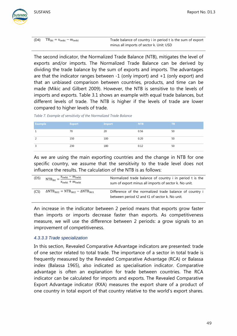
SUSFANS
Report No. D1.3
49
(D4) TBikt = xiwkt − miwkt Trade balance of country i in period t is the sum of export
minus all imports of sector k. Unit: USD
The second indicator, the Normalized Trade Balance (NTB), mitigates the level of
exports and/or imports. The Normalized Trade Balance can be derived by
dividing the trade balance by the sum of exports and imports. The advantages
are that the indicator ranges between -1 (only import) and +1 (only export) and
that an unbiased comparison between countries, products, and time can be
made (Mikic and Gilbert 2009). However, the NTB is sensitive to the levels of
imports and exports. Table 3.1 shows an example with equal trade balances, but
different levels of trade. The NTB is higher if the levels of trade are lower
compared to higher levels of trade.
Table 7. Example of sensitivity of the Normalized Trade Balance
Example Export Import NTB TB
1 70 20 0.56 50
2 150 100 0.20 50
3 230 180 0.12 50
As we are using the main exporting countries and the change in NTB for one
specific country, we assume that the sensitivity to the trade level does not
influence the results. The calculation of the NTB is as follows:
(D5) NTBikt =xiwkt − miwkt
xiwkt + miwkt Normalized trade balance of country i in period t is the
sum of export minus all imports of sector k. No unit.
(C5) ∆NTBikt2 = NTBikt2 − ∆NTBikt1 Difference of the normalized trade balance of country i
between period t2 and t1 of sector k. No unit.
An increase in the indicator between 2 period means that exports grow faster
than imports or imports decrease faster than exports. As competitiveness
measure, we will use the difference between 2 periods: a grow signals to an
improvement of competitiveness.
4.3.3.3 Trade specialization
In this section, Revealed Comparative Advantage indicators are presented: trade
of one sector related to total trade. The importance of a sector in total trade is
frequently measured by the Revealed Comparative Advantage (RCA) or Balassa
index (Balassa 1965), also indicated as specialisation indicator. Comparative
advantage is often an explanation for trade between countries. The RCA
indicator can be calculated for imports and exports. The Revealed Comparative
Export Advantage indicator (RXA) measures the export share of a product of
one country in total export of that country relative to the world’s export shares.

SUSFANS
Report No. D1.3
50
A RXA indicator of 1 indicates that exports of a product of the country is equally
specialized as the total world exports. A level below 1 means relatively
unspecialized and above 1 relatively specialized. The latter indicates an export
advantage, as relatively more of that product is exported than the world
average. In fact, it indicates the export focus of an industry and is therefore
externally oriented.
A first flaw of this indicator is that re-exporting might suggest high
competitiveness of one industry. These transit activities might be influenced by
a good performance of another sector i.e. logistics or by beneficial natural and
infrastructural conditions like sea or airports. This RXA indicator is often used in
competitiveness studies as sole indicator (Frohberg and Hartmann 1997, Fertö
and Hubbard 2003, Wijnands, Bremmers et al. 2008, Fischer 2010, Latruffe 2010,
Carraresi and Banterle 2015, Jambor and Babu 2016). A second flaw is that the
importance of the domestic market is neglected. A growing domestic demand
signals a good competitive performance that might go at the costs of exports;
the industry can grow with decreasing exports and even with decreasing
imports.
Despite these flaws, it might be considered to include this measure in the
analysis as it takes not only the exports of one product (such XS) but also the
comparative position of one product in the whole export portfolio of a country.
An alternative for RXA is the Additive Revealed Comparative Export Advantage
(ARXA)12. The ARXA indicator is not as common as the RXA. The ARXA is the
difference of the share of commodity in total exports of one country and the
share of the world in total. As each share is between 0 and 1 the difference will
be between -1 and +1 symmetric around zero. In fact, it measures the deviation
of a country of world’s total and by this indicating whether the country is less
(ARXA below zero) or more specialised (ARXA above zero). This indicator can be
interpreted more easily than the RXA. As competitiveness indicator, either the
RXA or the ARXA will be used: we prefer the more commonly used RXA.
(D6)
wt
kt
iwt
ikwt
ikt
XTX
xTx
RXA
Revealed Comparative Export Advantage (RXA) indicator
for sector k, country i in period t. No unit.
(C6) ∆RXAikt2 = RXAikt2 − RXAikt1 Growth RXA on the world market for sector k for country i
between period t2 and t1. No unit
12
The equation is as follows:
wt
kt
iwt
ikwtikt XT
XxT
xARXA
Additive Revealed Comparative Export Advantage
(ARXA) indicator for sector k, country i in period t.

SUSFANS
Report No. D1.3
51
The opposite of the revealed export advantage indicator is the revealed import
advantage (RMA). The interpretation of the indicator is reversed from that of
RXA. A value below unity (=1) shows that country imports relatively less than the
world average and can be indicated as a competitive advantage; a value above
unity indicates a relatively higher import level. High levels or re-export of
imported products, due to comparative advantage of other sectors or country’s
location, might explain a high value. This indicator as such is not an indicator for
assessing competitiveness and will only be used to calculate the Revealed Net
Trade Advantage (RTA).
(D7)
wt
kt
iwt
ikwt
ikt
MTM
mTm
RMA
Revealed Comparative Import Advantage (RMA) indicator
for sector k, country i in period t. No unit.
An indicator that combines the previous 2 indicators is the Revealed net Trade
Advantage (RTA) indicator. This is defined by Scott and Vollrath as difference
between the RXA and RMA (Scott and Vollrath 1992). It has an advantage above
the indicators based on either exports or imports as it includes both flows
(Frohberg and Hartmann 1997). A positive RTA indicates a competitive
advantage: exports exceed imports. Negative values indicate competitive
disadvantages (Scott and Vollrath 1992).
(D8) iktiktikt RMARXARTA
Revealed Net Trade Advantage (RTA) indicator for sector k,
country i in period t. No unit.
(C8) 122 iktiktikt RTARTARTA
Growth RTA of sector k for country i between period t2
and t1. No unit.
The Revealed Net Trade Advantage (RTA) indicators differ from the Normalized
Trade Balance and Openness indicators mentioned above in respect to product
orientation and the size of the economy. The RTA indicators take only the
revealed trade position of a specific sector compared with all sectors into
account. The Normalized Trade Balance and Openness are focused only on the
performance of a specific product of a country compared to size of the
economy. Therefore, both indicators are of importance.
The Michelaye Comparative Trade indicator (MRTA)13 is an alternative of the
RTA indicator, as it compares export shares with import shares of a specific
sector of a specific country (Mikic and Gilbert 2009). This indicator takes values
13
The equation is:
iwt
ikwt
iwt
ikwtikt mT
mxT
xMRTA
Michelaye Comparative Trade indicator (MRTA for
sector k, country i in period t.

SUSFANS
Report No. D1.3
52
between -1 and +1. If the value is negative, the country has a negative revealed
(export) comparative advantage and if positive, it has positive advantage. The
range between -1 and +1 enables a straightforward interpretation and is less
complex to derive than the RTA. The nominators are the aggregated world total
imports respectively the exports in theory these values should be on the same
level except logistics costs: hence, the indicator indicates the net-trade as share
in the total world trade. For consistency reason, we prefer the RTA indicator, as
it is derived from the often-used Balassa index.
4.3.4 Performance metric 3: Production (Economic performance
of a sector and productivity cross-sector benchmarking)
4.3.4.1 Economic performance of a sector
The European Council conclusion from 2000 set as strategic goals an economic
growth and more jobs (European Council 2000). In economics, creating added
value is an important indicator for economic growth and expresses industrial
dynamism. Value added is seen as a better indicator than turnover as turnover
includes also intermediate products, whereas value added is based on the
production factors labour, capital and land. As inflation differences between
countries will blur the real developments the nominal value added14, this
indicator has to be deflated. To derive the real value added at factor costs, the
nominal value added is deflated by the Food Price index, also indicated as food
inflation. However, this might be a preferred deflator for the food sector, it will
be less suitable for deflating the Gross production of Value added of all
economic activities of a country. For that reason, we choose the price inflation
(PI) of all goods.
(D9)
it
iktikt
PI
GVARVA
Real value added for sector k in in country i for period t. Unit:
USD
(C9)
1ikt
1ikt2ikt2ikt
RVA
RVARVARVA
Growth RVA of sector k for country i between period t2 and t1.
No unit.
This indicator as such, is not well suited as competitiveness measure. It is size
sensitive: large countries or countries with a large industry will have a large
value added. The derived variable is insensitive to size.
The derived variable above recognizes the economic growth. An obvious second
competitiveness variable will be the growth of the jobs. However, in the GTAP
model employment is not measured in persons but in monetary values. A
14
The inflation measures the change in the costs that the average consumer has to pay for a
basket for services and goods.
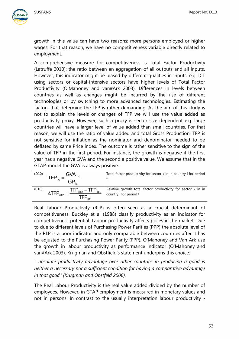
SUSFANS
Report No. D1.3
53
growth in this value can have two reasons: more persons employed or higher
wages. For that reason, we have no competitiveness variable directly related to
employment.
A comprehensive measure for competitiveness is Total Factor Productivity
(Latruffe 2010): the ratio between an aggregation of all outputs and all inputs.
However, this indicator might be biased by different qualities in inputs: e.g. ICT
using sectors or capital-intensive sectors have higher levels of Total Factor
Productivity (O'Mahoney and van#Ark 2003). Differences in levels between
countries as well as changes might be incurred by the use of different
technologies or by switching to more advanced technologies. Estimating the
factors that determine the TFP is rather demanding. As the aim of this study is
not to explain the levels or changes of TFP we will use the value added as
productivity proxy. However, such a proxy is sector size dependent e.g. large
countries will have a larger level of value added than small countries. For that
reason, we will use the ratio of value added and total Gross Production. TFP is
not sensitive for inflation as the nominator and denominator needed to be
deflated by same Price index. The outcome is rather sensitive to the sign of the
value of TFP in the first period. For instance, the growth is negative if the first
year has a negative GVA and the second a positive value. We assume that in the
GTAP-model the GVA is always positive.
(D10)
ikt
iktikt
GP
GVATFP
Total factor productivity for sector k in in country i for period
t
(C10)
1ikt
1ikt2ikt2ikt
TFP
TFPTFPTFP
Relative growth total factor productivity for sector k in in
country i for period t
Real Labour Productivity (RLP) is often seen as a crucial determinant of
competitiveness. Buckley et al (1988) classify productivity as an indicator for
competitiveness potential. Labour productivity affects prices in the market. Due
to due to different levels of Purchasing Power Parities (PPP) the absolute level of
the RLP is a poor indicator and only comparable between countries after it has
be adjusted to the Purchasing Power Parity (PPP). O’Mahoney and Van Ark use
the growth in labour productivity as performance indicator (O'Mahoney and
van#Ark 2003). Krugman and Obstfield’s statement underpins this choice:
‘...absolute productivity advantage over other countries in producing a good is
neither a necessary nor a sufficient condition for having a comparative advantage
in that good.’ (Krugman and Obstfeld 2006).
The Real Labour Productivity is the real value added divided by the number of
employees. However, in GTAP employment is measured in monetary values and
not in persons. In contrast to the usually interpretation labour productivity -

SUSFANS
Report No. D1.3
54
Value Added per unit labour input- now the labour productivity is the Value
Added per USD labour input. If the same deflator for employment will be used,
the monetary values do not need to be deflated; otherwise, the monetary value
of employment has to be deflated.
(D11)
ikt
iktikt
E
VARLP
Real labour productivity for sector k in in country i for period
t. Unit: USD VA per USD E
(C11)
1ikt
1ikt2ikt2ikt
RLP
RLPRLPRLP
Relative growth real labour productivity for sector k in in
country i for period t. Unit: USD VA per USD E
As productivity influences the prices on the final markets it can be seen as a cost
competitiveness indicator or price indicator. Several authors mention costs or
prices (unit value) as a competitiveness indicator (Buckley, Pass et al. 1988,
Durand, Simon et al. 1992, Marsh and Tokarick 1994). These data are often
linked to trade and domestic prices. The number of products from the
agribusiness or food sector is numerous and hence a unit value comparison for
one sector is almost impossible. A second disadvantage is that prices are
focussed on the competition on one specific market, benchmarking exporting
countries with the domestic production. In this case, cross-country comparison
is focussed on just one market. In our approach, we benchmark countries at the
world market. Due to difficulties to acquire adequate data and because of the
focus, we compare only productivity indicators instead of actual prices.
4.3.4.2 Productivity – cross sector benchmarking
Above we discussed the competitiveness on the final markets (either foreign or
domestic), in this section we focus on the competitiveness for means of
production. The comparative advantage of the three above mentioned
productivity indicators are considered to assess the competition for means of
production. Buckley et all. (1988) mentioned the “% manufacturing in total
output” as one of the performance indicators. This indicator covers the issue of
comparative advantage of a sector. In addition, we prefer the added value
above output or gross, following the approach of Wijnands et al. (Wijnands,
Bremmers et al. 2008, Wijnands and Verhoog 2016). Value added indicates the
rents on the production factors, whereas output (or turnover) might be the
result of large level of inputs or intermediary products. As competitiveness
indicator, we use not the absolute level but as for others the growth in the share
similar to the other measures. The derived variables (measures) are
straightforward.
For Value added:

SUSFANS
Report No. D1.3
55
(D12)
ibt
iktikt
RVA
RVARRVA
Ratio real value added for sector k in benchmark
sector b in country i for period t
(C12)
1ikt
1ikt2ikt2ikt
RRVA
RRVARRVARRVA
Relative growth ratio real value added for sector k
in in country i for period t
For Total Factor productivity:
(D13)
ibt
iktikt
TFP
TFPRTFP
Ratio real total factor productivity for sector k in
benchmark sector b in country i for period t
(C13)
1ikt
1ikt2ikt2ikt
RTFP
RTFPRTFPRTFP
Relative growth ratio total factor productivity for
sector k in in country i for period t
And for Real labour productivity:
(D14)
ibt
iktikt
RLP
RLPRRLP
Ratio real labour productivity k in benchmark
sector b in country i for period t
(C14)
1ikt
1ikt2ikt2ikt
RRLP
RRLPRRLPRRLP
Relative growth ratio real labour productivity for
sector k in in country i for period t
4.3.5 The aggregation pathway from variables to metrics
The policy goal for competitiveness is a relative value: the most competitive or
the best performing economy. For that reason, a value of an aggregate variable
(above indicated by C#) has to be benchmarked to assess its comparative
position. First, we present the data source. All individual variables (E-level) are
available or will be available from runs with the GTAP model.
We distinguish at least 3 periods:
t1 Actual base year of GTAP
t2 Future year based on a run of GTAP. For this period several scenarios can
be developed such as a baseline scenario (business as usual), full
liberalisation of trade, or abolishment of free trade agreements and so on.
t0 Year in the past, it is recommended that t1-t0 is equal to t2-t1 for which
similar GTAP data are available
A number of countries/regions are selected. These countries have to remain
identical for each assessment, as these countries serve as benchmark countries
for assessing the comparative position of each country on an aggregate variable
(C-level). For possibilities to select countries or regions see:
https://www.gtap.agecon.purdue.edu/databases/regions.asp?Version=9.211
SUSFANS
Report No. D1.3
56
A sector or a specific aggregation of sectors has to be chosen compliant with
GTAP classification. See:
https://www.gtap.agecon.purdue.edu/databases/contribute/detailedsector.asp.
We suggest to include some levels of the value chain e.g. producers, food
processors and retail. Furthermore, some large sectors e.g. the meat or dairy
sector might even be recognized in the analysis. The metrics allow each level of
sector detail, the selection of sectors depends on the overall aim of Susfans.
For each period, we have a set of aggregated variables for one sector covering
all selected countries. Hence, the number of observations is equal to the
number of selected countries. As competitiveness is a comparative concept, the
“policy target” is being the best performing country or region. The “policy
target” will therefore the maximum of the observations. This policy target differs
for each period, each variable and scenario. If in t2 several scenarios are
evaluated, the policy target will have to be determined for each scenario. With
this information, the performance indicator at SUSFANS B-level can be derived.
The performance metrics is the comparative position of a sector of a country in
a period and is indicated by the symbols ∆* and are derived from the
competitiveness measures with the symbol ∆. In Table 4.1 we suggest to take
the average: a weighted average can be considered. The variables ∆* and the
overall performance indicator A-level can be derived by following the SUSFANS
metrics approac

SUSFANS
Report No. D1.3
57
Table 8. Performance metrics for Policy Goal: ‘Competitiveness of EU agri-food business’
Policy goals Performance metrics (assessable against targets; B derived from C)
Aggregate indicators (C, derived from D) Derived variable (D, derived from E) Individual variable (E)
Competitiveness
of EU Food
System
Production and trade Difference of the openness of country i between period t2 and t1 of sector k. Unit % (C1)
Openness of country i for sector k. Unit: % (D1)
xijkt, mijkt, GPikt, Difference of the Self-sufficiency ratio of country i between period t2 and t1 of sector k. Unit % (C2)
Self–Sufficiency ratio of the country i for sector k. Unit: % (D2)
Trade - Export flow orientation Growth export share on the world market for sector k for country i between period t2 and t1. No unit (C3)
Export share of country i of sector k to the world (w) in year t. No unit (D3)
xijkt, xiwkt, miwkt,
xTiwt, Xkt, XTwt,
mTiwt, MTwt,
Trade - Trade orientation Trade balance of country i in period t is the sum of export minus all imports of sector k. Unit: USD (D4)
Difference of the normalized trade balance of country i between period t2 and t1 of sector k. No unit. (C5)
Normalized trade balance of country i in period t is the sum of export minus all imports of sector k. No unit. (D5)
Trade - Trade specialization Growth RXA on the world market for sector k for country i between period t2 and t1. No unit (C6)
Revealed Comparative Export Advantage (RXA) indicator for sector k, country i in period t. No unit. (D6)
Revealed Comparative Import Advantage (RMA) indicator for sector k, country i in period t. No unit. (D7)
Growth RTA of sector k for country i between period t2 and t1. No unit. (C8)
Revealed Net Trade Advantage (RTA) indicator for sector k, country i in period t. No unit. (D8)
Production - Economic performance of a sector
Growth RVA of sector k for country i between period t2 and t1. No unit. (C9)
Real value added for sector k in in country i for period t. Unit: USD (D9)
GVAikt, PIit, GPikt, Vaikt, Eikt, GVAibt, GPibt, VAibt, Eibt
Relative growth total factor productivity for sector k in in country i for period t (C10)
Total factor productivity for sector k in in country i for period t (D10)
Relative growth real labour productivity for sector k in in country i for period t. Unit: USD VA per USD E (C11)
Real labour productivity for sector k in in country i for period t. Unit: USD VA per USD E (D11)
Production - Productivity cross-sector benchmarking
Relative growth ratio real value added for sector k in in country i for period t (C12)
Ratio real value added for sector k in benchmark sector b in country i for period t (D12)
Relative growth ratio total factor productivity for sector k in in country i for period t (C13)
Ratio real total factor productivity for sector k in benchmark sector b in country i for period t (D13)
Relative growth ratio real labour productivity for sector k in in country i for period t (C14)
Ratio real labour productivity k in benchmark sector b in country i for period t (D14)

SUSFANS
Report No. D1.3
58
4.4 Policy goal: Equitable outcomes and conditions of
the EU food system
Equity considerations are an intrinsic element of the food security discourse and
have been propagated strongly by those who address food security as a basic
human right. Since the seminal publications of Amartya Sen in the 1980s, it is
commonly understood that food insecurity must be understood in a wide
socioeconomic and cultural context, which deprives people from the
opportunities to consume the food in the quantities and quality that they want
and need.
Since the early 1990s, the number of people suffering from undernourishment
decreased from about 1,011 million (19% of world population) to 795 million
people (11% of world population) in 2014-2016 (FAO, 2015). On the one hand,
this reduction reflects progress made in the fight against hunger; on the other
hand, it shows that inequity among people who manage and people who do
not manage to meet their food and health needs is still significant. This inequity
is related to the daily living conditions of people: the social, economic and
political conditions in which people are born, grow, live, work, and age (Friel and
Baker, 2009). Hungry people are faced with daily living conditions that hamper
them to grow sufficient food for themselves or to earn enough income to meet
their food and health needs (Mulvany and Ensor, 2011).
Food and nutrition security (FNS) is a European problem as much as it is a
global challenge, but with EU-specific features. The main challenge in the EU is
the impact of poor diets on the disease burdens, i.e. the prevalence of both
undernutrition and rising overweight and obesity. Both are to a large extent
driven by socio-economic exclusion in the food system and other forms of
inequity: the poor, ethnic minorities and the elderly are particularly vulnerable
groups within the EU. Geographically, the FNS challenges are concentrated in
the Eastern member states of the EU, where problems of poor food
environments compound with compromised access to fresh and nutritious food
products, in particular fruit and vegetables (Cockx, Francken and Pieters, 2015;
Rizov, Cupak and Pokrivcak, 2015; Alexandri, Alexandri, Păuna and Luca , 2016).
A growing number of people relies on food banks (Hebinck and Villarreal, 2016).
In general, there is a need to analyse the quality of the food environment across
the EU and its relation to the consumption choices, nutrition outcomes and
health burdens from diet-related diseases.
The EU food system structure, policies of EU and member states related to food
and agriculture and the various outcomes of the EU food system have a
significant impact on how people around the world are able to meet their food

SUSFANS
Report No. D1.3
59
requirements. This consideration led the SUSFANS team to formulate a fourth
policy goal related to global FNS to capture how the EU impacts on global FNS.
In consultation with the stakeholder core group of the project (SCG) this policy
goal was broadened as stakeholders felt that the project should address a wider
array of equity issues related to the EU food system as well. Stakeholders
participating in the first two SCG workshops questioned how issues related to
equity within in the food system, such as power relationships between food
system actors, participation in decision-making or fair wages, and with respect
to the food system outcomes, e.g. food poverty in the EU or global FNS, could
be included in the analysis and therefore in the selection of metrics to assess
SFNS. Earlier stakeholder consultations on policy visions and scenarios on global
food and nutrition security presented similar interests (de Bakker et al., 2017).
The SUSFANS team thus broadened the fourth policy goal and renamed it
‘Equitable outcomes and conditions of the EU food system’. Different from the
three other policy goals the Equity goal has not been formulated in detail within
the context of metrics for FNS before and the project team is here breaking new
ground in order to establish a set of meaningful metrics. For that the SUSFANS
team is also consulting with experts outside of the project that work on equity
considerations15. In addition, an internet survey and further probing with the
stakeholder core group are planned to discuss the proposed metrics and
indicators as these could not be discussed before in the two SCG workshops.
Thus the list presented here is still indicative of the final list. In the consultations
also the full set of metrics will be reviewed once more in order to establish if the
full set of performance metrics for SFNS consists for the right mix and is
formulated in a way that is easy to communicate.
Equity considerations are duly enshrined in the European treaties. A priori,
however, there is no level or state of equity in society that will maximize social
welfare. Equity itself is not known to have been the objective of a particular
public policy. Public policies and programs are known to focus on addressing
income inequalities, social exclusion and discrimination and lack of power or
voice. These efforts contribute to greater equity in society rather than that they
aim to deliver on a particular vision on what equity is desirable. That is a
significant conceptual challenge for the design of performance metrics on
equity in the food system. The policy targets against which to assess indicators
on equity in the conditions and outcomes of food systems are missing.
15
The SUSFANS team held a small workshop with experts from the Centre of Agroecology,
Water and Resilience of the Coventry University, UK, where various team members work on
issues such as food sovereignty, gender issues in food systems etc. This workshop helped to
develop a first list of possible variables and indicators to consider and the SUSFANS team would
like to gratefully acknowledge their contributions.

SUSFANS
Report No. D1.3
60
For a proper analysis of equity in SFNS it is proposed to include equities in daily
living conditions of social groups, equities in the extent to which social groups
are able to meet their food needs, and health equities among social groups. By
doing so both causes (i.e. inequities in daily living conditions), direct results (i.e.
inequities in meeting food needs) and indirect results (health inequities) can be
taken into account. In this section some suggestions for the design of equity
metrics for FNS are given. This design is built upon the various elements of the
SUSFANS SFNS conceptual framework and covers equities in daily living
conditions, meeting food needs and health. The metrics only reflect quantitative
and qualitative inequities among social groups in relative terms without giving
any value judgment.
Equity can be measured among actors within a country or between actors in
different countries. Which option is applied depends on the purpose of the
analysis. As SUSFANS is focussed on FNS in the EU in relation to global impacts,
SUSFANS equity indicators are collected at country level in order to compare
equity of actors in different countries, both between EU countries and between
EU and non-EU countries.
Equity indicators can be expressed in absolute and relative terms. Most
indicators on meeting food needs will be given in absolute terms, from which it
is easy to assess the distance from the level of fully satisfying the need. On the
other hand, most indicators on daily living conditions and health are given in
relative terms, often as share of the population. It has to be noted that such
shares can be expressed in both positive terms and negative terms, i.e. the share
of population having more than 1$ a day and the share of population having
less than 1$ a day. As we aim to construct aggregate indicators we have to take
care that these are based on individual equity variables that are expressed in the
same way: either negative or positive. In SUSFANS we express equity variables in
negative terms. This implies that low shares are associated with more equity
than higher shares.
In Table 10 a hierarchy of indicators for the equity policy goal is presented. The
solution to overcome the challenge of addressing policy targets is pragmatically
addressed case by case.
4.4.1 Performance metric 1: Equity among food chain actors and
primary producers
The SUSFANS conceptual framework (D1.1) distinguishes between the
conditions and structure of the food system and the outcomes of the system.
This distinction is an important one for guiding the analysis of equity
considerations for the food system. The conditions and structure are related to

SUSFANS
Report No. D1.3
61
how the different actors in the system deal with each other and who holds the
power within the system for deciding on the conditions in which food system
actors, such as the primary producers and the food chain actors, carry out their
activities. In order to capture the equity aspects in the conditions and structure
of the food system, the SUSFANS team formulated a performance metric called
‘Equity among food chain actors and primary producers’, which aims to measure
the extent of fair conditions in access to resources (land, capital, etc.) for
producers and chain actors. The access to resources was seen as a tangible
measure for understanding the structure of the EU food system and the
distribution of power within the system. Three aggregate indicators were
selected to measure these issues in more detail. The first one is the ‘Access to
resources for primary producers’, which can be derived from variables such as
the ‘Share of farmers without legal ownership of farm land’ and the ‘Share of
female farmers without access to agricultural land’. The second Aggregate
Indicator is the ‘Access to finance and technology’, derived from variables such
as the ‘Share of farmers without access to microfinance’, the ‘Share of farm
women without access to savings and credit’ and the ‘Share of farmers without
primary education’ and the ‘Share of farmers without access to vocational
training’. The third Aggregate Indicator is called ‘Fair trading practices’ which
aims to capture power relationships in the EU food system by using the ‘Share
of farmers who are faced with a monopolistic downstream industry’ and the
‘Share of farmers who are faced with a monopolistic upstream industry’ as the
variables to describe this issue in more detail.
4.4.2 Performance metric 2: Equity among consumers: food
system conditions
Also among consumers a number of conditions of the food system determine if
different parts of the population have equitable access to food. Three
Aggregate Indicators were selected that can describe the performance metric of
‘Equity among consumers: food system conditions’ and therefore show a picture
of the conditions within which consumers are able to obtain food. The first
Aggregate Indicator is called ‘Wealth’, which can be derived from the following
variables ‘National income per capita by region as percentage of the EU national
income per capita’, ‘Household income per capita by region as % of EU
household income per capita’, ‘Share of the population with less than 1$ a day’,
‘Share of the population that has no access to health care centres’, ‘Share of the
population without access to sanitation facilities’ and ‘Share of the female
population without primary education’. The second Aggregate Indicator used
here is supposed to portray ‘Political stability’ as derived from the ‘Share of the
population living in political unstable conditions’, the ‘Share of the population

SUSFANS
Report No. D1.3
62
without right to social security’ and the ‘Share of the population that has no
access of safety nets such as food assistance or pensions’. The third Aggregate
Indicator that can determine food access is called ‘Consumer choices’ and
results from the two following variables, namely ‘Share of the population
without access to fresh food’ and ‘Share of the population whose food
preferences are not met by food supply’.
4.4.3 Performance metric 3: Equity among consumers: food
system outcomes
With respect to the outcomes of the food system the project considers here
both the classical set of indicators for FNS as they are presented in the food
security literature (availability, accessibility, utilization and stability) together
with indicators measuring the health outcomes of the food system. For the FNS
indicators the SUSFANS project bases its selection of variables on the work of
the EU project FOODSECURE (www.foodsecure.eu) (Shutes et al. forthcoming). A
summary of the available FNS Aggregate Indicators and their associated
variables is provided in Table 9. Food and nutrition security indicators and the
type of consumer and the scale in which they can be assessed
9. The variables have been developed based on the FAO suite of FNS indicators
(FAO, 2016) as part of the FOODSECURE project.16 A selection of the indicators
have been used to evaluate food and nutrition security in four stakeholder
developed visions of the future (see Shutes et al., 2017 for further details). The
metrics presented in this section have been designed to match the data and
model indicators in two assessment tools, i.e. the MAGNET model of
Wageningen Economic Research and the GLOBIOM model of the International
Institute for Applied Systems Analysis (IIASA).
Aggregate Indicator: Availability
Derived Variable: Calorie availability
This Derived Variable gives the total amount of net (kilo)calories available per
capita per day for the average consumer globally, within the EU and non-EU
regions and at the member states level. The indicator will also be available for
different household types in the case study countries, giving insight into
variations within these countries. The indicator is defined as the total calories
imported and produced for domestic human consumption and therefore
exclude calories in food exports and those in animal feed and biofuel
feedstocks. The unit of this indicator is kilocalories per capita per day.
16
The results of the FOODSECURE project, including an assessment of future scenarios for food
and nutrition in the EU and globally, are available via the website www.foodsecure.eu/navigator.

SUSFANS
Report No. D1.3
63
Table 9. Food and nutrition security indicators and the type of consumer and the scale in which they can be
assessed
Type of consumer and scale
FNS
Dimension
Derived Variable Average consumer
worldwide, EU,
non-EU and
member state level
Household specific
values in case study
countries
Availability Calorie availability
Availability Share of nutritious food
Availability Reduction in share of protein of animal origin
Availability Domestic food production n/a
Accessibility Share of food expenditure in total expenditures
Accessibility National income per capita n/a
Accessibility Food affordability n/a
Accessibility Household income per capita
Accessibility Consumption per capita
Utilisation Share of calories from fruit and vegetables
Stability Cereal import dependency ratio n/a
Stability Value of food imports over total merchandise
exports
n/a
Stability Market pressure index EU n/a
Source: EU project FOODSECURE, except for the market pressure index which is an original
contribution of SUSFANS.
Derived Variable: Share of nutritious foods
The share of nutritious foods is defined as 1 minus the share of energy
(kilocalories) derived from cereals (MAGNET17) or cereals, roots and tubers
(GLOBIOM), where the calories from cereals or cereals, roots and tubers is the
percentage share of total calories available for consumption. The unit for this
indicator is percent.
Derived Variable: Reduction in share of protein of animal origin
This indicator focuses on the share of protein from animal origin (including or
excluding fish) in total protein. The indicator is constructed so that an increase
represents a reduction in protein from animal sources, reflecting the average
over-consumption of protein in the European diet. Caution should be taken
when interpreting this variable in relation to low-income countries where
(animal) protein consumption may be below optimal levels.
17
Roots and tubers are combined with fruit and vegetables in the MAGNET database.

SUSFANS
Report No. D1.3
64
Derived Variable: Domestic food production
The average value of primary food production is an indicator of the strength of
the domestic food producing sector. It is defined over primary food rather than
including food processing as it relates to the food availability dimension of food
and nutrition security. The variable is defined per capita in constant (2010)
prices.
Aggregate Indicator: Accessibility
Derived Variable: Share of non-food expenditure in total expenditures
The share of non-food expenditure in total expenditures is 1 minus the share of
food spending in total spending for the average household. Higher shares of
non-food expenditure in total expenditure are associated with higher food
security as changes in food prices and incomes have less of a direct impact on
food consumption i.e. they are insulated by having non-food income that can
be diverted to food if necessary. This variable is also available by household
type in the case study regions. The unit for this indicator is percent and excludes
savings.
Derived Variable: National income per capita
National income per capita gives an indication of the wealth of a nation. It is
measured as GDP per capita in constant US dollars.
Derived Variable: Food affordability
Food affordability is indicated by the real domestic primary food price index.
The index can also be expanded to include processed food and weighted by
consumption to reflect how price changes affect the average consumer and
household types with different consumption baskets. In the latter case, the
variable becomes household specific as common prices affect households
different due to the different weights of food products in total food
consumption.
Derived Variable: Household income per capita
Household income per capita is a further measure of wealth in a region which
can be household specific due to different patterns of factor incomes in
different household types. At the household level, the variable also accounts for
different rates of population growth.
Derived Variable: Consumption per capita
Average and household specific food consumption per capita shows how
changes in prices, incomes and population combine to affect food consumption.

SUSFANS
Report No. D1.3
65
The variable is a Paasche volume index of food consumption which includes
primary and processed foods.
Aggregate Indicator: Utilisation
Derived Variable: Share of calories from fruit and vegetables
The standard FAO utilisation indicators centre on measures of physical
development (e.g. stunting and wasting), health outcomes (e.g. anaemia) and
water and sanitation. Given the limitation of economic models to inform these
indicators, we introduce the share of calories from fruit and vegetables as a
crude proxy for a healthy diet and micronutrient intake. The variable includes
vegetables and fruits consumed directly, via processed products and via food
services. The variable is expressed as a percentage of total calories consumed.
Aggregate Indicator: Stability
Derived Variable: Cereal import dependency ratio
This variable shows the degree to which a country or region is dependent on
cereal imports. The variable is bounded at zero so all net exporters take this
value. The variable is expressed as a percentage.
Derived Variable: Value of food imports over total merchandise exports
This variable provides a measure of vulnerability and captures the adequacy of
foreign exchange reserves to pay for food imports, which has implications for
national food security depending on production and trade patterns (FAO, 2016).
FAO definition excludes fish which is included here. The variable is expressed as
a percentage.
Derived Variable: Market pressure index
The volatility of agricultural markets has a profound impact on food and nutrition security (Kalkuhl, von Braun and Torero, 2017). For a given agricultural commodity, the market pressure index provides the percent difference between the actual price and the predicted price based on market fundamentals, macroeconomic and financial developments, as well as the dynamics of climatic variables (Crespo Cuarisma, Hlouskova and Obersteiner, 2017). The forecasting model used to obtain the predictions is chosen after an exhaustive scrutiny of the predictive ability of a large number of state-of-the-art multivariate time series specifications and combinations thereof. The index indicates whether the prevalent climatic and economic conditions are expected to lead to an increase or a decrease of the price of a particular agricultural commodity at a given horizon (from one to twelve months ahead) and by how much the price is expected to change.
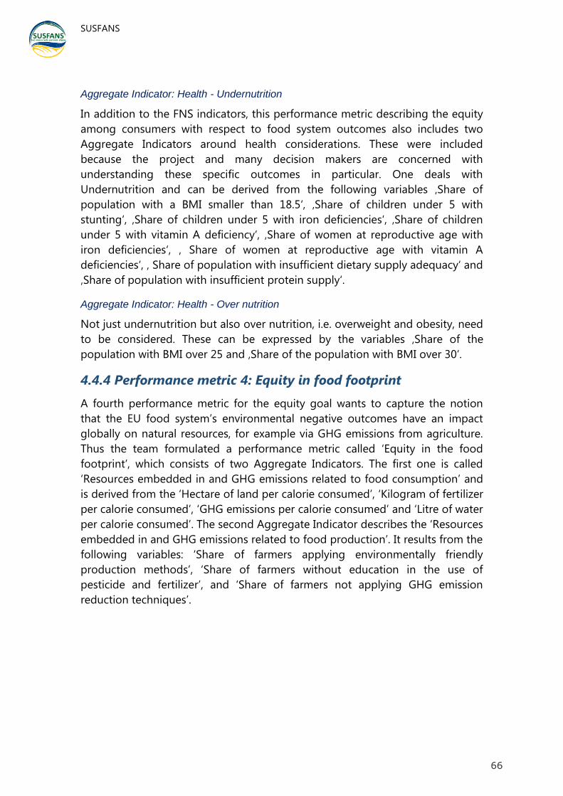
SUSFANS
Report No. D1.3
66
Aggregate Indicator: Health - Undernutrition
In addition to the FNS indicators, this performance metric describing the equity
among consumers with respect to food system outcomes also includes two
Aggregate Indicators around health considerations. These were included
because the project and many decision makers are concerned with
understanding these specific outcomes in particular. One deals with
Undernutrition and can be derived from the following variables ‚Share of
population with a BMI smaller than 18.5‘, ‚Share of children under 5 with
stunting‘, ‚Share of children under 5 with iron deficiencies‘, ‚Share of children
under 5 with vitamin A deficiency‘, ‚Share of women at reproductive age with
iron deficiencies‘, ‚ Share of women at reproductive age with vitamin A
deficiencies‘, ‚ Share of population with insufficient dietary supply adequacy‘ and
‚Share of population with insufficient protein supply‘.
Aggregate Indicator: Health - Over nutrition
Not just undernutrition but also over nutrition, i.e. overweight and obesity, need
to be considered. These can be expressed by the variables ‚Share of the
population with BMI over 25 and ‚Share of the population with BMI over 30‘.
4.4.4 Performance metric 4: Equity in food footprint
A fourth performance metric for the equity goal wants to capture the notion
that the EU food system’s environmental negative outcomes have an impact
globally on natural resources, for example via GHG emissions from agriculture.
Thus the team formulated a performance metric called ‘Equity in the food
footprint’, which consists of two Aggregate Indicators. The first one is called
‘Resources embedded in and GHG emissions related to food consumption’ and
is derived from the ‘Hectare of land per calorie consumed’, ‘Kilogram of fertilizer
per calorie consumed’, ‘GHG emissions per calorie consumed’ and ‘Litre of water
per calorie consumed’. The second Aggregate Indicator describes the ‘Resources
embedded in and GHG emissions related to food production’. It results from the
following variables: ‘Share of farmers applying environmentally friendly
production methods’, ‘Share of farmers without education in the use of
pesticide and fertilizer’, and ‘Share of farmers not applying GHG emission
reduction techniques’.

SUSFANS Report No. D1.3
67
Table 10. Performance metrics for Policy Goal: 'Equitable outcomes and conditions'
Policy goal Performance
metric
Aggregate indicator Derived variable International data
source1)
Equity Equity among consumers: food system outcomes
Availability Calorie availability by region (EU, non-EU) MAGNET
Share of nutritious food by region (EU, non-EU) MAGNET
Reduction in share of protein of animal origin by region (EU, non-EU) MAGNET
Domestic food production per capita by region (EU, non-EU) MAGNET
Accessibility Share of food expenditure in total expenditures by region (EU, non-EU) MAGNET
Food affordability by region (EU, non-EU) MAGNET
Consumption per capita by region (EU, non-EU) MAGNET
Utilization Share of calories from fruit and vegetables by region (EU, non-EU) MAGNET
Stability Cereal import dependency ratio by region (EU, non-EU) MAGNET
Value of food imports over total merchandise exports by region (EU, non-EU) MAGNET
Market pressure index ApriPrice
Health: Undernutrition
Share of population with BMI <18.5
Share of children < 5 years with stunting WHO/UNICEF
Share of children < 5 years with iron deficiency WHO/UNICEF
Share of children < 5 years with vitamin A deficiency WHO/UNICEF
Share of women at reproductive age with iron deficiency WHO/UNICEF
Share of women at reproductive age with vitamin A deficiency WHO/UNICEF
Share of population with insufficient dietary supply adequacy FAO
Share of population with insufficient protein supply FAO
Health: Overweight and obesity Share of population with BMI >25
Share of population with BMI >30
Equity among consumers: food system conditions
Wealth National income per capita by region as % of EU national income per capita MAGNET
Household income per capita by region as % of EU household income per capita MAGNET
Share of population with less than 1$ a day World Bank
Share of population that has no access to a health care center World Bank
Share of population without access to sanitation facilities World Bank
Share of female population without primary education
Political stability Share of population living in a political unstable surrounding
Share of population without right to social security FAO
Share of population that has no access to a safety net (food assistance, pension)

SUSFANS Report No. D1.3
68
Consumer choices Share of population without access to a fresh food shop
Share of population whose food preferences are not met by food supply
Equity among producers and chain actors
Access to resources by primary
producers
Share of farmers without legal status of ownership of the farm land
Share of farm women without access to agricultural land
Access to finance and technology Share of farmers without access to microfinance World Bank
Share of farm women without access to saving and credit World Bank
Share of farmers without primary education
Share of farmers without access to vocational training
Fair trading practices Share of farmers who are faced with a monopolist downstream industry
Share of farmers who are faced with a monopolist upstream industry
Equity food footprint Resources embedded in and emissions
related to food consumption
Ha of land per calorie consumed MAGNET
Kg of fertilizer per calorie consumed MAGNET
Litre of water per calorie consumed
Unit of emissions per calorie consumed
Resources embedded in and emissions
related to food production
Share of farmers applying environmentally friendly production methods
Share of farmers without education in the use of pesticides and fertilizers
Share of farmers not applying emission reducing techniques
Pangaribowo et al. (2013) have identified data sources for some of the indicators. Other indicators have to be derived from individual studies.

SUSFANS
Report No. D1.3
69
5. CONCLUSION AND OUTLOOK
Assessing the status for the EU food system with respect to its various outcomes is a
complex undertaking. The SUSFANS team developed an approach to derive a small
set of high level performance metrics describing the four SUSFANS policy goals from
a much larger number of variables and indicators. The full list of metrics for each goal
can be found in Table 11. This approach should allow policy and decision makers
concerned with different parts of the whole EU food system to make sense of trends
that are becoming visible in the present but also to think about possible innovations
to move the EU food system closer towards sustainability and thus in the direction of
the four outlined policy goals. These innovation options and possibilities for food
system change are explored in more detail in WP5 as well as W6 and WP10. The
metrics presented here allows the assessment of these proposed options. That said in
this first step to metric selection presented here the current set up of the
performance metrics only allows an assessment within each policy goal but not yet
with a view across all four goals at the same time.
In a next step, the team is exploring which of the models of the SUSFANS tool box
can estimate which ones of the performance metrics. This assessment of the model
capabilities will also yield a better understanding of which performance metrics will
have to be aggregated and estimated using qualitative methods in addition to
describing which linkages across the models might have to be built. Deliverable D1.4
will describe the modelling strategy in more detail.
In a second step the SUSFANS team will bring all performance metrics together in an
integrated set that will allow a view across all four policy goals and thus across all
aspects of SFNS. The proposed method for doing this will be described in D1.5. To
this end, the performance metrics will be presented in form of a spider diagram
(Figure 2) showing where the EU currently stands on the selected metrics for all four
policy goals. The diagram will also allow a visualisation of the potential impacts of
different policy interventions. The aim is to offer the spider diagram in easily-
accessible on-line format whereby users can gauge overall impact or access specific
areas of interest in greater detail. It will also be possible to examine an entire next
level of detail across the spider diagram by clicking on a given performance metrics
to expand that section of the diagram and illustrate the indicators, variables and the
aggregation pathway. Overall aim of presenting the performance metrics in this way
is to give decision makers the option to not only see how a proposed food system
innovation (e.g. introduction of insect protein) would fare with respect to achieving a
more balanced diet but also what consequences this intervention would for the other
policy goals. Thus the diagram could be used to visualize the unintended
consequences of an intervention together with the expected outcomes.

SUSFANS
Report No. D1.3
70
Figure 2 Proposed integrated set of metrics for assessing SFNS of the EU food system
In order to make the proposed integration tool, i.e. the spider diagram, as user
friendly as possible the project will hold a round of consultations with the SCG of the
project. This will be done via a web based survey and a webinar to elicit stakeholder
options on how they see the metrics set fitting into their decision making processes.
Stakeholders will be also consulted on the current set of Equity metrics as these have
been developed only since the last stakeholder meeting.
One challenge that the SUSFANS team will still have to address in the work on the
metrics and the integration tool is how different stakeholders or groups of consumer
will prioritize the various performance metrics in their decision making processes.
Each actor is likely to give a different weighting to the policy goals and thus to the
metrics describing these. Also, it is likely that consumer groups across different
countries will differ in their priorities with respect to the food system outcomes, e.g.

SUSFANS
Report No. D1.3
71
prioritizing social outcomes over environmental ones. Thus the project team is aiming
to find a way how stakeholders can ‘play’ with the weights given to different metrics.
An additional challenge is to ensure that the integrated metrics tool is flexible
enough to allow the integration of new insights from the project’s and external work
into its metrics hierarchy and also accommodate shifting policy priorities across
different stakeholder groups. For the pilot application developed for D1.5 the team
will see if these aspects can already be addressed.

SUSFANS Report No. D1.3
72
Table 11. The complete set of SUSFANS performance metrics and their associated indicators and variables.
POLICY
GOALS
Performance metrics
(assessable against targets; B
derived from C)
Aggregate indicators
(C, derived from D)
Derived variable
(D, derived from E)
Individual variable
(E)
Balanced and
sufficient diet
for EU citizens’
Food based summary score
based on 5 key foods (0-100):
Fruits
Vegetables
Fish
Red & Processed meat intake
Sugar Sweetened Beverages (SSB)
N.A.
Vegetables Legumes (Unsalted) nuts and seeds Fruits Fish
Dairy Red/ processed meat Hard cheese Sugar sweetened beverages Alcohol Salt
Intake of >10 food products have
been individually assessed in
country specific population
surveys and have been aligned
with FoodEx2 classification
system

SUSFANS Report No. D1.3
73
Nutrient based summary score
(0-100)
NRD 9.3
NRD 15.3
N.A.
NRD 9.3 includes protein, dietary fibre,
calcium, iron, potassium, magnesium,
and vitamin A, C and E, saturated fat,
added sugar, and sodium.
NRD 15.3 additionally includes mono-
unsaturated fatty acids, zinc, vitamin D
and B-vitamins (B1, B2, B12, folate), but
excludes magnesium.
Energy
Protein
Mono-
unsaturated
fat
Fibre
Calcium
Iron
Magnesium
Potassium
Selenium
Iodine
Zinc
Vitamin A
Vitamin C
Vitamin E
Vitamin B1
Vitamin B2
Vitamin B6
Vitamin B12
Folate
Vitamin D
Sodium
Saturated fat
Total sugar
Protein, plant
Protein, animal
Saturated Fatty
Acids (SFA)
Mono-
Unsaturated
Fatty Acids
(MUFA)
Poly-
Unsaturated
Fatty Acids
(PUFA)
Energy balance
% of population with normal
weight: 100% is ‘ideal’
BMI (kg/m2):
normal weight: 18.5–24.9
overweight: 25–29.9
obese:>30 kg/m2
BMI (body mass index of each
country)
Reduction of
environmental
impacts Climate stabilization
Reduction of total GHG emissions
caused by the agri-food chain
CO2 eq
CO2, CH4, N2O (Emissions
according to IPCC categories incl.
indirect land use change, per unit
of product in food consumed
(LCA) = C footprints)
Use/emissions of cooling agents
in fish production (CFCs, …)
Radiative Forcing Land Cover (e.g. albedo)

SUSFANS Report No. D1.3
74
Clean air and water
Reduction of N surplus Nitrogen surplus
N input (fertiliser, manure,
atmospheric deposition,
biological fixation, feed) and N
output (yield), change of soil
stocks. Maybe split of N surplus
into emissions to the
atmosphere: air pollution and
emissions to the hydrosphere:
water pollution)
Reduction of N emissions to the
atmosphere (air pollution)
Emissions of Nr to the atmosphere (NH3,
NOx) Emissions of NH3, NOx
Reduction of N emissions to the
hydrosphere (water pollution)
Emissions of Nr to the hydrosphere
(Nitrates, Organic N)
Emissions of NH3, NOx
Emissions of NO3, other run-off,
leaching
Reduction of P surplus Phosphorus surplus P input and output
Reduction of Toxic substances use Toxic substances use Use of toxic substances
(pesticides, …)
Biodiversity conservation
Reduction of the contribution of the
agrifood chain to loss of Mean Species
Abundance (MSA)
Contribution to loss of Mean Species
Abundance (MSA) calculated with the
GLOBIO model (Alkemade et al., 2009)
Land use
Emissions of GHGs, Nr
Land use
Land use (Shannon) The Shannon’s entropy index (Hr)
seafloor area impacted (m2)
Protected areas (GLOBIOM) Land use map
Species rich hotspots (GLOBIOM) Land use map
Reduction in number of threatened
species Red List Index (RLI)
IUCN Red List threat status
(terrestrial and marine) of
affected species
Preservation of natural
resources
Sustainable water use [e.g. maintenance
of environmental flows] Terrestrial water scarcity footprint
Irrigation water use
Water use in livestock production
Water use in the food chain
Water supply
Sustainable exploitation of wild-caught
seafood resources
distance to optimum exploitation
(F/FMSY) Fishing mortality (F)

SUSFANS Report No. D1.3
75
%PPR relative to total available
ecosystem production
primary production required
(PPR)
Maintenance of soil fertility Soil degradation Erosion
Soil carbon contents
Competitiveness
of EU agri-food
business Production and trade
Difference of the openness of country i
between period t2 and t1 of sector k.
Unit % (C1)
Openness of country i for sector k. Unit:
% (D1)
xijkt, mijkt, GPikt, Difference of the Self-sufficiency ratio of
country i between period t2 and t1 of
sector k. Unit % (C2)
Self–Sufficiency ratio of the country i
for sector k. Unit: % (D2)
Trade - Export flow orientation
Growth export share on the world
market for sector k for country i
between period t2 and t1. No unit (C3)
Export share of country i of sector k to
the world (w) in year t. No unit (D3)
xijkt, xiwkt, miwkt, xTiwt, Xkt, XTwt, mTiwt,
MTwt,
Trade - Trade orientation
Trade balance of country i in period t is
the sum of export minus all imports of
sector k. Unit: USD (D4)
Difference of the normalized trade
balance of country i between period t2
and t1 of sector k. No unit. (C5)
Normalized trade balance of country i in
period t is the sum of export minus all
imports of sector k. No unit. (D5)
Trade - Trade specialization
Growth RXA on the world market for
sector k for country i between period t2
and t1. No unit (C6)
Revealed Comparative Export
Advantage (RXA) indicator for sector k,
country i in period t. No unit. (D6)
Revealed Comparative Import
Advantage (RMA) indicator for sector k,
country i in period t. No unit. (D7)
Growth RTA of sector k for country i
between period t2 and t1. No unit. (C8)
Revealed Net Trade Advantage (RTA)
indicator for sector k, country i in period
t. No unit. (D8)
Production - Economic
performance of a sector
Growth RVA of sector k for country i
between period t2 and t1. No unit. (C9)
Real value added for sector k in in
country i for period t. Unit: USD (D9) GVAikt, PIit, GPikt, Vaikt, Eikt, GVAibt,
GPibt, VAibt, Eibt Relative growth total factor productivity
for sector k in in country i for period t
(C10)
Total factor productivity for sector k in
in country i for period t (D10)

SUSFANS Report No. D1.3
76
Relative growth real labour productivity
for sector k in in country i for period t.
Unit: USD VA per USD E (C11)
Real labour productivity for sector k in in
country i for period t. Unit: USD VA per
USD E (D11)
Production - Productivity cross-
sector benchmarking
Relative growth ratio real value added
for sector k in in country i for period t
(C12)
Ratio real value added for sector k in
benchmark sector b in country i for
period t (D12)
Relative growth ratio total factor
productivity for sector k in in country i
for period t (C13)
Ratio real total factor productivity for
sector k in benchmark sector b in
country i for period t (D13)
Relative growth ratio real labour
productivity for sector k in in country i
for period t (C14)
Ratio real labour productivity k in
benchmark sector b in country i for
period t (D14)
Equitable
outcomes and
conditions
Equity among consumers: food
system outcomes
Availability
Calorie availability by region (EU, non-
EU)
MAGNET
Share of nutritious food by region (EU,
non-EU)
MAGNET
Reduction in share of protein of animal
origin by region (EU, non-EU)
MAGNET
Domestic food production per capita by
region (EU, non-EU)
MAGNET
Accessibility
Share of food expenditure in total
expenditures by region (EU, non-EU)
MAGNET
Food affordability by region (EU, non-EU) MAGNET
Consumption per capita by region (EU,
non-EU)
MAGNET
Utilization Share of calories from fruit and
vegetables by region (EU, non-EU)
MAGNET
Stability
Cereal import dependency ratio by
region (EU, non-EU)
MAGNET
Value of food imports over total
merchandise exports by region (EU, non-
EU)
MAGNET
Market pressure index AgriPrice

SUSFANS Report No. D1.3
77
Health: Undernutrition
Share of population with BMI <18.5
Share of children < 5 years with stunting WHO/UNICEF
Share of children < 5 years with iron
deficiency
WHO/UNICEF
Share of children < 5 years with vitamin
A deficiency
WHO/UNICEF
Share of women at reproductive age
with iron deficiency
WHO/UNICEF
Share of women at reproductive age
with vitamin A deficiency
WHO/UNICEF
Share of population with insufficient
dietary supply adequacy
FAO
Share of population with insufficient
protein supply
FAO
Health: Overweight and obesity Share of population with BMI >25
Share of population with BMI >30
Equity among consumers: food
system conditions
Wealth
National income per capita by region as
% of EU national income per capita
MAGNET
Household income per capita by region
as % of EU household income per capita
MAGNET
Share of population with less than 1$ a
day
World Bank
Share of population that has no access
to a health care centre
World Bank
Share of population without access to
sanitation facilities
World Bank
Share of female population without
primary education
Political stability
Share of population living in a political
unstable surrounding
Share of population without right to
social security
FAO

SUSFANS Report No. D1.3
78
Share of population that has no access
to a safety net (food assistance, pension)
Consumer choices
Share of population without access to a
fresh food shop
Share of population whose food
preferences are not met by food supply
Equity among producers and
chain actors
Access to resources by primary
producers
Share of farmers without legal status of
ownership of the farm land
Share of farm women without access to
agricultural land
Access to finance and technology
Share of farmers without access to
microfinance
World Bank
Share of farm women without access to
saving and credit
World Bank
Share of farmers without primary
education
Share of farmers without access to
vocational training
Producer sovereignty
Share of farmers who are faced with a
monopolist downstream industry
Share of farmers who are faced with a
monopolist upstream industry
Equity in food footprint
Resources embedded in and emissions
related to food consumption
Ha of land per calorie consumed MAGNET
Kg of fertilizer per calorie consumed MAGNET
Litre of water per calorie consumed
Unit of emissions per calorie consumed
Resources embedded in and emissions
related to food production
Share of farmers applying no organic
production methods
Share of farmers without education in
the use of pesticides and fertilizers
Share of farmers not applying emission
reducing techniques

SUSFANS
Report No. D1.3
I
REFERENCES
‘Alkama, R. and A. Cescatti (2016). "Biophysical climate impacts of recent changes in global
forest cover." Science 351(6273): 600-604.
Ablove, T, et al. (2015) Body mass index continues to accurately predict percent body fat as
women age despite changes in muscle mass and height. Menopause, 22(7): p. 727-30.
Acharya, T., J. Fanzo, D. Gustafson, J. Ingram, B. Schneeman, L. Allen, K. Boote, A. Drewnowski, F.
Ewert and S. Hall (2014). "Assessing sustainable nutrition security: the role of food
systems." Center for Integrated Modeling of Sustainable Agriculture and Nutrition
Security. Washington, DC.
Alkemade, R., M. Oorschot, L. Miles, C. Nellemann, M. Bakkenes and B. ten Brink (2009).
"GLOBIO3: A Framework to Investigate Options for Reducing Global Terrestrial
Biodiversity Loss." Ecosystems 12(3): 374-390.
Allen, T. and P. Prosperi (2014). "Metrics of Sustainable Diets and Food Systems. Workshop
Report. Bioversity International & CIHEAM-IAMM. Montpellier, France.".
Allen, T., P. Prosperi, B. Cogill and G. Flichman (2014). "Agricultural biodiversity, social-ecological
systems and sustainable diets." Proceedings of the Nutrition Society 73: 498-508.
Balassa, B. (1965). "Trade liberalisation and “revealed” comparative advantage." The Manchester
School 33(2): 99-123.
Ballard, T. J., A. W. Kepple and C. Cafiero (2013). "The food insecurity experience scale:
development of a global standard for monitoring hunger worldwide. Technical Paper.
Rome, FAO. Retrieved from: http://www.fao.org/economic/ess/ess-fs/voices/en/."
Bradbury, KE, et al. (2017) Association between physical activity and body fat percentage, with
adjustment for BMI: a large cross-sectional analysis of UK Biobank. BMJ Open, 7(3): p.
e011843.
Buckley, P. J., C. L. Pass and K. Prescott (1988). "Measures of international competitiveness: A
critical survey." Journal of marketing management 4(2): 175-200.
Butchart, S. H. M., A. J. Stattersfield, J. Baillie, L. A. Bennun, S. N. Stuart, H. R. Akcakaya, C. Hilton-
Taylor and G. M. Mace (2005). "Using Red List Indices to measure progress towards the
2010 target and beyond." Philosophical Transactions of the Royal Society B: Biological
Sciences 360(1454): 255-268.
Butchart, S. H. M., M. Walpole, B. Collen, A. van Strien, J. P. W. Scharlemann, R. E. A. Almond, J. E.
M. Baillie, B. Bomhard, C. Brown, J. Bruno, K. E. Carpenter, G. M. Carr, J. Chanson, A. M.
Chenery, J. Csirke, N. C. Davidson, F. Dentener, M. Foster, A. Galli, J. N. Galloway, P.
Genovesi, R. D. Gregory, M. Hockings, V. Kapos, J. F. Lamarque, F. Leverington, J. Loh, M.
A. McGeoch, L. McRae, A. Minasyan, M. H. Morcillo, T. E. E. Oldfield, D. Pauly, S. Quader,
C. Revenga, J. R. Sauer, B. Skolnik, D. Spear, D. Stanwell-Smith, S. N. Stuart, A. Symes, M.
Tierney, T. D. Tyrrell, J. C. Vie and R. Watson (2010). "Global Biodiversity: Indicators of
Recent Declines." Science 328(5982): 1164-1168.

SUSFANS
Report No. D1.3
II
Čapková, N, Lustigová, M, Kratěnová, J, Žejglicová, K (2016): (in Czech) Zdravotní stav české
populace – výsledky studie EHES. Státní zdravotní ústav, 2016, 32 s. ISBN 978-80-7071-
356-3.
Carlton, D. W. and J. M. Perloff (1999). Modem industrial organization. Reading, Massachusetts,
Addison-Wesley.
Carraresi, L. and A. Banterle (2015). "Agri-food Competitive Performance in EU Countries: A
Fifteen-Year Retrospective." International Food and Agribusiness Management Review
18(2): 37.
CFS. (2012). "Coming to Terms with Terminology: Food Security, Nutrition Security, Food
Security and Nutrition, Food and Nutrition Security." Thirty-ninth Session Retrieved 4
August, 2016, from http://www.fao.org/docrep/meeting/026/MD776E.pdf.
Christensen, V., S. Guenette, J. J. Heymans, C. J. Walters, R. Watson, D. Zeller and D. Pauly (2003).
"Hundred-year decline of North Atlantic predatory fishes." Fish and Fisheries 4(1): 1-24.
Clapp, J. (2014). "Food security and food sovereignty: Getting past the binary." Dialogues in
Human Geography 4(2): 206-211.
Coll, M., S. Libralato, S. Tudela, I. Palomera and F. Pranovi (2008). "Ecosystem Overfishing in the
Ocean." PLoS ONE 3(12): e3881-e3881.
Crouch, G. I. and J. B. Ritchie (1999). "Tourism, competitiveness, and societal prosperity." Journal
of business research 44(3): 137-152.
Cuaresma, Jesus Crespo, Jaroslava Hlouskova, and Michael Obersteiner. “Forecasting
Commodity Prices Under Specification Uncertainty: A Comprehensive Approach.” SUSFANS
Deliverable D8.3, 2017. http://www.susfans.org/portfolio/deliverable-83-forecasting-
commodity-prices-under-specification-uncertainty-comprehensive
De Bakker, Erik, Michiel van der Werff, Michiel van Dijk, Thom Achterbosch. “Shifting governance
visions on global food and nutrition security: Lessons from the FOODSECURE
stakeholder scenario approach.” FOODSECURE working paper no. 59. The Hague: LEI
Wageningen UR. May 2017
De Vries, W., J. Kros, G. J. Reinds and K. Butterbach-Bahl (2011). "Quantifying impacts of nitrogen
use in European agriculture on global warming potential." Current Opinion in
Environmental Sustainability 3(5): 291-302.
Diana, J. S. (2009). "Aquaculture Production and Biodiversity Conservation." BioScience 59(1): 27-
38.
Dise, N. B., M. Ashmore, S. Belyazid, A. Bleeker, R. Bobbink, W. de Vries, J. W. Erisman, T.
Spranger, C. J. Stevensand and L. van den Berg (2011). Nitrogen as a threat to European
terrestrial biodiversity. M. Sutton, C. Howard, J. W. Erisman et al. Cambridge, Cambridge
University Press. 333: 463-494.
Drewnowski, A (2005). Concept of a nutritious food: toward a nutrient density score." The
American J Clin Nutr 82(4): 721-732.

SUSFANS
Report No. D1.3
III
Drewnowski, A (2009). Defining nutrient density: development and validation of the nutrient rich
foods index." Journal of the American College of Nutrition 28(4): 421S-426S.
Drury, C. M. (2013). Management and cost accounting, Springer.
Dulvy, N. K., Y. Sadovy and J. D. Reynolds (2003). "Extinction vulnerability in marine populations."
Fish and Fisheries 4(1): 25-64.
Durand, M., J. Simon and C. Webb (1992). "OECD's indicators of international trade and
competitiveness."
Ec (1991). "Council Directive of 12 December 1991 concerning the protection of waters against
pollution caused by nitrates from agricultural sources (91/676/EEC)."
Ec (2001). "Directive 2001/81/EC of the European Parliament and of the Council of 23 October
2001 on national emission ceilings fo rcertain atmospheric pollutants." Official Journal of
the European Communities 2001L0081(October 2001): 22-30.
Eea (2015). Annual European Union greenhouse gas inventory 1990–2013 and inventory report
2015. EEA Technical report No. 19/2015. Luxembourg, Publications Office of the
European Union.
EFSA - European Food Safety Authority (2010). Scientific Opinion on principles for deriving and
applying Dietary Reference Values. EFSA Journal 2010 8(3): 1458.
EFSA - European Food Safety Authority (2014). Guidance on the EU Menu methodology. EFSA
Journal 2014;12(12):3944
Emeis, K.-C., J. van Beusekom, U. Callies, R. Ebinghaus, A. Kannen, G. Kraus, I. Kröncke, H. Lenhart,
I. Lorkowski, V. Matthias, C. Möllmann, J. Pätsch, M. Scharfe, H. Thomas, R. Weisse and E.
Zorita (2015). "The North Sea — A shelf sea in the Anthropocene." Journal of Marine
Systems 141: 18-33.
Eu (2000). "Directive 2000/60/EC of the European Parliament and of the Council of 23 October
2000 establishing a framework for Community action in the field of water policy."
Official Journal of European Union L327.
Eu (2008). "Directive 2008/56/EC of the European Parliament and of the Council of 17 June 2008
establishing a framework for community action in the field of marine environmental
policy (Marine Strategy Framework Directive) (Text with EEA relevance)." Official Journal
of European Union L164.
Eu (2013). "Regulation (EU) No 1305/2013 of the European Parliament and of the Council of 17
December 2013 on support for rural develoment by the European Agricultural Fund for
Rural Development (EAFRD) and repealing Council Regulation (EC) No 1698/2005."
Official Journal of the European Union L 347: 487-548.
Eu (2013). "Regulation (EU) No 1306/2013 of the European Parliament and of the Council of 17
December 2013 on the financing, management and monitoring of the common
agricultural policy and repealing Council Regulations (EEC) No 352/78, (EC) No 165/94,
(EC) No 2799/98." Official Journal of the European Union L 347: 549-607.

SUSFANS
Report No. D1.3
IV
Eu (2013). "Regulation (EU) No 1307/2013 of the European Parliament and of the Council of 17
December 2013 establishing rules for direct payments to farmers under support
schemes within the framework of the common agricultural policy and repealing Council
Regulation." Official Journal of the European Union L 347: 608-670.
Eu (2014). Facts and figures on the Common Fisheries Policy. Basic statistical data. 2014 Edition.
Eu (2016). "Directive (EU) 2016/2284 of the European Parliament and of the Council of 14
December 2016 on the reduction of national emissions of certain atmospheric
pollutants, amending Directive 2003/35/EC and repealing Directive 2001/81/EC (Text
with EEA relevance." Official Journal of European Union L344.
European, C. (2011). "COM(2011)112 final. Communication from the European Parliament, the
Council, the European Economic and Social Committee and the Committee of the
Regions. A Roadmap for moving to a competitive low carbon economy in 2050." Official
Journal of European Union.
European, C. (2011). "COM/2011/0244 final. Communication from the Commission to the
European Parliament, the Council, the Economic and Social Committee and the
Committee of the Regions: Our life insurance, our natural capital: an EU biodiversity
strategy to 2020." (2011): 17-17.
European, C. (2013). Communication from the Commission to the European Parliament, the
Council, the European Economic and Social committee and the Committee of the
Regions. A Clean Air Programme for Europe.
European, C. (2014). Communication from the Commission to the European Parliament, the
Council, the European Economic and Social Committee and the Committee of the
Regions. A policy framework for climate and energy in the period from 2020 to 2030.
COM(2014) 15 final.
European, U. (2015). "Council Decision (EU) 2015/1339 of 13 July 2015 on the conclusion, on
behalf of the European Union, of the Doha Amendment to the Kyoto Protocol to the
United Nations Framework Convention on Climate Change and the joint fulfilment of
commitments thereunder." Official Journal of the European Union L2017.
European#Council (2000). Presidency conclusions, Lisbon European Council. 23 and 24 march
2000.
FAO (2015). The state of food insecurity in the world 2015. Rome.
FAO (2016). Food security indicators.
Fao (2016). The State of World Fisheries and Aquaculture 2016. Rome, Food and Agriculture
Organization of the United Nations.
FAO. (2016). "FAO Statistical Pocket Book." Retrieved 21-06-2016, 2016, from
http://www.fao.org/docrep/016/i2493e/i2493e06.pdf.
Fertö, I. and L. J. Hubbard (2003). "Revealed Comparative Advantage and Competitiveness in
Hungarian Agri–Food Sectors." The World Economy 26(2): 247–259.

SUSFANS
Report No. D1.3
V
Fischer, C. (2010). "Food quality and product export performance: an empirical investigation of
the EU situation." Journal of International Food & Agribusiness Marketing 22(3-4): 210-
233.
Fischer, C. G. and T. Garnett (2016). "Plates, pyramids and planets: Developments in national
healthy and sustainable dietary guidelines: a state of play assessment. FAO and The
Food Climate Research Network at The University of Oxford.".
Flegal, K.M., et al., Comparisons of percentage body fat, body mass index, waist circumference,
and waist-stature ratio in adults. Am J Clin Nutr, 2009. 89(2): p. 500-8.
Fleisher, C. S. and B. E. Bensoussan (2003). Strategic and competitive analysis: methods and
techniques for analyzing business competition, Prentice Hall Upper Saddle River, NJ.
Friel, S. and P. I. Baker (2009). "Equity, food security and health equity in the Asia Pacific region."
Asia Pac J Clin Nutr 18(4): 620-632.
Frohberg, K. and M. Hartmann (1997). Comparing measures of competitveness. Halle, Institute of
Agricultural Development in Central and Eastern Europe.
Fulgoni VL, Keast DR, Drewnowski A (2009) Development and validation of the nutrient-rich
foods index: a tool to measure nutritional quality of foods. J Nutr. Aug;139:1549-54.
Garnier, J., A. Beusen, V. Thieu, G. Billen and L. Bouwman (2010). "N:P:Si nutrient export ratios
and ecological consequences in coastal seas evaluated by the ICEP approach." Global
Biogeochemical Cycles 24: GB0A05-GB00A05.
Global Panel (2015). "Improved metrics and data are needed for effective food system policies in
the post-2015 era. Technical Brief. London, UK. Global Panel on Agriculture and Food
Systems for Nutrition.".
Gorton, M., C. Hubbard and I. Fertő (2013). Theoretical background and conceptual framework.
Halle, Leibniz Institute of Agricultural Development in Transition Economies (IAMO).
Grizzetti, B., F. Bouraoui and A. Aloe (2012). "Changes of nitrogen and phosphorus loads to
European seas." Global Change Biology 18(2): 769-782.
Grizzetti, B., F. Bouraoui, G. Billen, H. van Grinsven, A. C. Cardoso, V. Thieu, J. Garnier, C. Curtis, R.
W. Howarth and P. J. Johnes (2011). Nitrogen as a threat to European water quality. M.
Sutton, C. Howard, J. W. Erisman et al. Cambridge, Cambridge University Press: 379-404.
Gudmundsson, H. (2003). "The Policy Use of Environmental Indicators - Learning from Evaluation
Research." The Journal of Transdisciplinary Environmental Studies 2(2): 1-12.
Gustafson, D., A. Gutman, W. Leet, A. Drewnowski, J. Fanzo and J. Ingram (2016). "Seven food
system metrics of sustainable nutrition security." Sustainability 8(3): 1-17.
Halpern, B. S., C. Longo, J. S. S. Lowndes, B. D. Best, M. Frazier, S. K. Katona, K. M. Kleisner, A. A.
Rosenberg, C. Scarborough and E. R. Selig (2015). "Patterns and Emerging Trends in
Global Ocean Health." PLOS ONE 10(3): e0117863-e0117863.

SUSFANS
Report No. D1.3
VI
Hamel, G. and C. K. Prahalad (1994). Competing for the future: Breakthrough strategies for
seizing control of your industries and creating the markets of tomorrow. Harvard,
Harvard Business School Press.
Hansen, J., M. Sato, P. Kharecha, D. Beerling, R. Berner, V. Masson-Delmotte, M. Pagani, M.
Raymo, D. L. Royer and J. C. Zachos (2008). "Target Atmospheric CO2: Where Should
Humanity Aim?" The Open Atmospheric Science Journal 2(1): 217-231.
Hebinck, A. and Villarreal G. (2016) ‘Local’ level analysis of FNS pathways the Netherlands.
Exploring two case studies: Urban Food Initiatives and Food Bank practices. Wageningen
University, TRANSMANGO project.
http://transmango.eu/userfiles/update%2009112016/reports/5%20the%20netherlands%
20report.pdf.
Henderson, A. (2015). Eutrophication. M. Z. Hauschild and M. A. J. Huijbregts. Dordrecht,
Springer Netherlands: 177-196.
Hoekstra, A. Y., A. K. Chapagain, M. M. Aldaya and M. M. Mekonnen (2011). The Water Footprint
Assessment Manual. Setting the global standard. London, earthscan.
Howarth, L. M., C. M. Roberts, R. H. Thurstan and B. D. Stewart (2014). "The unintended
consequences of simplifying the sea: making the case for complexity." Fish and Fisheries
15(4): 690-711.
Ingram, J. (2011). "A food systems approach to researching food security and its interactions
with global environmental change." Food Security 3(4): 417-431.
Ipcc (2006). 2006 IPCC Guidelines for National Greenhouse Gas Inventories, Prepared by the
National Greenhouse Gas Inventories Programme - Volume 4 Agriculture, Forestry and
Other Land Use. Japan, IGES.
Ipcc (2014). "Climate Change 2014 Synthesis Report Summary Chapter for Policymakers." Ipcc:
31-31.
Jambor, A. and S. Babu (2016). Competitiveness: Definitions, Theories and Measurement.
Competitiveness of Global Agriculture, Springer: 25-45.
Kram, T. and E. Stehfest (2012). The IMAGE model suite used for the OECD Environmental
Outlook to 2050. Bilthoven, PBL Netherlands Environmental Assessment Agency.
Krugman, P. (1994). "Competitiveness: a dangerous obsession." FOREIGN AFFAIRS-NEW YORK-
73: 28-28.
Krugman, P. R. and M. Obstfeld (2006). International Economics: Theory and Policy. Boston,
Pearson/Addison-Wesley.
Kalkuhl, Matthias, Joachim von Braun, and Maximo Torero, eds. Food Price Volatility and Its
Implications for Food Security and Policy. Cham: Springer Open, 2016.
Lal, R. (2016). "Beyond COP 21: Potential and challenges of the "4 per Thousand" initiative."
Journal of Soil and Water Conservation 71(1): 20A-25A.

SUSFANS
Report No. D1.3
VII
Latruffe, L. (2010). Competitiveness, Productivity and Efficiency in the Agricultural and Agri-Food
Sectors”, OECD Food, Agriculture and Fisheries Working Papers No. 30. Paris, OECD
Publishing.
Le Vallée, J.-C. and M. Grant (2016). "Canada’s Food Report Card 2015: International
Comparison. Ottowa: The Conference Board of Canada, 2016."
Lehtonen, M. (2015). Indicators: tools for informing, monitoring or controlling? The Tools of
Policy Formulation: Actors, Capacities, Venues and Effects. A. J. Jordan and J. R.
Turnpenny, Edward Elgar Publishing Ltd.
Lehtonen, M., L. Sébastien and T. Bauler (2016). "The multiple roles of sustainability indicators in
informational governance: between intended use and unanticipated influence." Current
Opinion in Environmental Sustainability 18: 1-9.
Leip, A., B. Achermann, G. Billen, A. Bleeker, A. Bouwman, W. de Vries, U. Dragosits, U. Doring, D.
Fernall, M. Geupel, J. Herolstab, P. Johnes, L. Gall, A. Christine, S. Monni, R. Neveceral, L.
Orlandini, M. Prud'homme, H. Reuter, D. Simpson, G. Seufert, T. Spranger, M. Sutton, J.
van Aardenne, M. Voss and W. Winiwarter (2011). "Integrating nitrogen fluxes at the
European scale." The European Nitrogen Assessment 5(2009): 345-376.
Leip, A., G. Billen, J. Garnier, B. Grizzetti, L. Lassaletta, S. Reis, D. Simpson, M. a. Sutton, W. de
Vries, F. Weiss and H. Westhoek (2015). "Impacts of European livestock production:
nitrogen, sulphur, phosphorus and greenhouse gas emissions, land-use, water
eutrophication and biodiversity." Environmental Research Letters 10(11): 115004-
115004.
Leip, A., M. Bielza, C. Bulgheroni, P. Ciaian, M. Lamboni, M.-l. Paracchini, J.-m. Terres, F. Weiss
and H.-p. Witzke Spatially Explicit Evaluation of the Agri - environmental Impact of CAP.
Lenzen, M., D. Moran, K. Kanemoto, B. Foran, L. Lobefaro and A. Geschke (2012). "International
trade drives biodiversity threats in developing nations." Nature 486(7401): 109-112.
Lewison, R., L. Crowder, A. Read and S. Freeman (2004). "Understanding impacts of fisheries
bycatch on marine megafauna." Trends in Ecology & Evolution 19(11): 598-604.
Lukas, M., H. Rohn, M. Lettenmeier, C. Liedtke and K. Wiesen (2016). "The nutritional footprint -
integrated methodology using environmental and health indicators to indicate potential
for absolute reduction of natural resource use in the field of food and nutrition." Journal
of Cleaner Production 132: 161-170.
Mace (2001). "A new role for MSY in single-species and ecosystem approaches to fisheries stock
assessment and management." Fish and Fisheries 2(1): 2-32.
Maes, J., C. Liquete, A. Teller, M. Erhard, M. L. Paracchini, J. I. Barredo, B. Grizzetti, A. Cardoso, F.
Somma, J.-E. Petersen, A. Meiner, E. R. Gelabert, N. Zal, P. Kristensen, A. Bastrup-Birk, K.
Biala, C. Piroddi, B. Egoh, P. Degeorges, C. Fiorina, F. Santos-Martín, V. Naruševičius, J.
Verboven, H. M. Pereira, J. Bengtsson, K. Gocheva, C. Marta-Pedroso, T. Snäll, C.
Estreguil, J. San-Miguel-Ayanz, M. Pérez-Soba, A. Grêt-Regamey, A. I. Lillebø, D. A.
Malak, S. Condé, J. Moen, B. Czúcz, E. G. Drakou, G. Zulian and C. Lavalle (2016). "An

SUSFANS
Report No. D1.3
VIII
indicator framework for assessing ecosystem services in support of the EU Biodiversity
Strategy to 2020." Ecosystem Services 17: 14-23.
Maggio, A., T. Van Cricking and J. P. Malingreau (2015). "Global Food Security 2030: assessing
trends with a view to guiding future EU policies." Joint Research Centre Foresight and
Behavioural Insights Unit, Science and Policy Reports.
Marchal, P., J. L. Andersen, M. Aranda, M. Fitzpatrick, L. Goti, O. Guyader, G. Haraldsson, A.
Hatcher, T. J. Hegland, P. Le Floc'h, C. Macher, L. Malvarosa, C. D. Maravelias, S. Mardle,
A. Murillas, J. R. Nielsen, R. Sabatella, A. D. M. Smith, K. Stokes, T. Thoegersen and C.
Ulrich (2016). "A comparative review of fisheries management experiences in the
European Union and in other countries worldwide: Iceland, Australia, and New Zealand."
Fish and Fisheries 17(3): 803-824.
Marsh, I. W. and S. Tokarick (1994). "Competitiveness indicators: a theoretical and empirical
assessment."
Mekonnen, M. M. and a. Y. Hoekstra (2011). "The green, blue and grey water footprint of crops
and derived crop products." Hydrology and Earth System Sciences 15(5): 1577-1600.
Metcalfe, J. S., L. Georghiou, P. Cunningham and H. M. Cameron (1992). Evaluation of the impact
of European Community research programmes upon the competitiveness of European
industry-Concepts and approaches. EUR 14198 EN. Research evaluation. Science and
Technology Policy Series.
Mikic, M. and J. Gilbert (2009). Trade Statistics in Policymaking-A handbook of commonly used
trade indices and indicators.
Mozaffarian, D. and D.S. Ludwig, Dietary guidelines in the 21st century--a time for food. JAMA,
2010. 304(6): p. 681-2.
Mulvany, P. and J. Ensor (2011). "Changing a dysfunctional food system: Towards ecological
food provision in the framework of food sovereignty." Food chain 1(1).
O'Mahoney, M. and B. van#Ark (2003). EU-productivity and competitiveness: an industry
perspective. Luxembourg, Office for Official Publication of the European Community:
273.
Pangaribowo, E., N. Gerber and M. Torero (2013). Food and Nutrition Security Indicators: A
Review, LEI Wageningen UR.
Pelletier, N. and A. Leip (2014). "Quantifying anthropogenic mobilization, flows (in product
systems) and emissions of fixed nitrogen in process-based environmental life cycle
assessment: rationale, methods and application to a life cycle inventory." The
International Journal of Life Cycle Assessment 19(1): 166-173.
Pfister, S. and P. Bayer (2014). "Monthly water stress: spatially and temporally explicit
consumptive water footprint of global crop production." Journal of Cleaner Production
73: 52-62.
SUSFANS
Report No. D1.3
IX
Pinsky, M. L., O. P. Jensen, D. Ricard and S. R. Palumbi (2011). "Unexpected patterns of fisheries
collapse in the world's oceans." Proceedings of the National Academy of Sciences
108(20): 8317-8322.
Pinstrup-andersen, P. (2009). "Food security : definition and measurement." Food Security 1: 5-7.
Popp, A., K. Calvin, S. Fujimori, P. Havlik, F. Humpenöder, E. Stehfest, B. L. Bodirsky, J. P. Dietrich,
J. C. Doelmann, M. Gusti, T. Hasegawa, P. Kyle, M. Obersteiner, A. Tabeau, K. Takahashi,
H. Valin, S. Waldhoff, I. Weindl, M. Wise, E. Kriegler, H. Lotze-Campen, O. Fricko, K. Riahi
and D. P. v. Vuuren (2017). "Land-use futures in the shared socio-economic pathways."
Global Environmental Change 42: 331-345.
Porter, M. E. (1980). Competitive strategy: Techniques for Analyzing Industries and Competitiors.
New York, The Free Press.
Porter, M. E. (1990). The competitive advantage of nations. London, The MacMillam Press Ltd.
Prosperi, P., T. Allen, M. Padilla, I. Peri and B. Cogill (2014). "Sustainability and Food & Nutrition
Security: A Vulnerability Assessment Framework for the Mediterranean Region." SAGE
Open 4(2).
Ranasinghe, C., et al., Relationship between Body Mass Index (BMI) and body fat percentage,
estimated by bioelectrical impedance, in a group of Sri Lankan adults: a cross sectional
study. BMC Public Health, 2013. 13: p. 797.
Ranganathan, J., D. Vennard, R. Waite, P. Dumas, B. Lipinski and T. Searchinger (2016). "Shifting
diets for a sustainable food future. World Resources Institute. Installment 11 of “Creating
a Sustainable Food Future”."
Redding, M. R., R. Lewis, T. Kearton and O. Smith (2016). "Manure and sorbent fertilisers increase
on-going nutrient availability relative to conventional fertilisers." Science of The Total
Environment 569-570: 927-936.
Reid, R. S., C. Bedelian, M. Y. Said, R. L. Kruska, R. M. Mauricio, V. Castel, J. Olson and P. K.
Thornton (2010). Global Livestock Impacts on Biodiversity. H. Steinfeld, H. A. Mooney, F.
Schneider and L. E. Neville. Washington DC, Scientific Committee on Problems of the
Environment (SCOPE); Island Press: 111-137.
Rockström, J., W. Steffen, K. Noone, Å. Persson, F. S. Chapin, E. Lambin, T. M. Lenton, M. Scheffer,
C. Folke, H. J. Schellnhuber, B. Nykvist, C. A. de Wit, T. Hughes, S. van der Leeuw, H.
Rodhe, S. Sörlin, P. K. Snyder, R. Costanza, U. Svedin, M. Falkenmark, L. Karlberg, R. W.
Corell, V. J. Fabry, J. Hansen, B. Walker, D. Liverman, K. Richardson, P. Crutzen and J.
Foley (2009). "Planetary boundaries: Exploring the safe operating space for humanity."
Ecology and Society 14(2).
Rogelj, J., M. den Elzen, N. Höhne, T. Fransen, H. Fekete, H. Winkler, R. Schaeffer, F. Sha, K. Riahi
and M. Meinshausen (2016). "Paris Agreement climate proposals need a boost to keep
warming well below 2 °C." Nature 534(7609): 631-639.
Röös, E., et al. (2015). "Evaluating the sustainability of diets–combining environmental and
nutritional aspects." Environmental Science & Policy 47: 157-166.

SUSFANS
Report No. D1.3
X
Rosenström, U. and J. Lyytimäki (2006). "The role of indicators in improving timeliness of
international environmental reports." European Environment 16(1): 32-44.
Sagheer, S., S. S. Yadav and S. G. Deshmukh (2009). "Developing a conceptual framework for
assessing competitiveness of India's agrifood chain." International Journal of Emerging
Markets 4(2): 137-159.
Schewe, J., J. Heinke, D. Gerten, I. Haddeland, N. W. Arnell, D. B. Clark, R. Dankers, S. Eisner, B. M.
Fekete, F. J. Colón-González, S. N. Gosling, H. Kim, X. Liu, Y. Masaki, F. T. Portmann, Y.
Satoh, T. Stacke, Q. Tang, Y. Wada, D. Wisser, T. Albrecht, K. Frieler, F. Piontek, L.
Warszawski and P. Kabat (2014). "Multimodel assessment of water scarcity under climate
change." Proceedings of the National Academy of Sciences 111(9): 3245-3250.
Schwab, K. (2014). The Global Competitiveness Report 2014–2015. Geneva, World Economic
Forum.
Scott, L. and T. Vollrath (1992). Global Competitive Advantages and Overall Bilateral
Complementarity in Agriculture: A Statistical Review. Washington, Economic Research
Service,U.S. Department of Agriculture.
Sen, A. (1981). Poverty and Famines: An Essay on Entitlement and Deprivation, Oxford:
Clarendon Press, New York: Oxford.
Shutes, L., H. Valin, E. Stehfest, M. v. Dijk, M. Kuiper, H. v. Meijl, A. Tabeau, M. Verma, D.
Oudendag, W.-J. v. Zeist and P. Havlik. (2017). Food and Nutrition Security and
Sustainability in Long-Term Projections: An Assessment of the FoodSecure Scenarios.
Paper prepared as part of Deliverable 7.4 of the FoodSecure project, foodsecure.eu.
Shutes, L., H.eE. Stehfest, M. van Dijk, M. Kuiper, H. van Meijl, A. Tabeau, M. Verma, D.
Oudendag, W.-J. van Zeist and P.Havlik, forthcoming, Food and Nutrition Security and
Sustainability in Long-Term Projections: An Assessment of the FoodSecure Scenarios.
FoodSecure working paper, foodsecure.eu
Siggel, E. (2006). "International competitiveness and comparative advantage: a survey and a
proposal for measurement." Journal of Industry, Competition and Trade 6(2): 137-159.
Siudek, T. and A. Zawojska (2014). "Competitiveness in the economic concepts, theories and
empirical research." Acta Scientiarum Polonorum. Oeconomia 13(1).
Spence, A. M. and H. A. Hazard (1998). International Competitiveness. Cambridge, MA, Ballinger
Publishing Company.
Steffen, W., K. Richardson, J. Rockström, S. Cornell, I. Fetzer, E. Bennett, R. Biggs and S. Carpenter
(2015). "Planetary boundaries: Guiding human development on a changing planet."
Science (New York, N.Y.) 348(6240): 1217-1217.
Stevens, C. J., C. Duprè, E. Dorland, C. Gaudnik, D. J. G. Gowing, A. Bleeker, M. Diekmann, D.
Alard, R. Bobbink, D. Fowler, E. Corcket, J. O. Mountford, V. Vandvik, P. A. Aarrestad, S.
Muller and N. B. Dise (2010). "Nitrogen deposition threatens species richness of
grasslands across Europe." Environmental pollution 158(9): 2940-2945.
SUN (2010). "A Road Map for Scaling-Up Nutrition." First edition.
SUSFANS
Report No. D1.3
XI
Terres, J.-M., B. Allen, W. Britz, C. Bulgheroni, J. Dwyer and M. L. Paracchini (2012). "WP5 Rural
Development - Indicators. Deliverable 5.2 of the project CAPRI-RD (Common
Agricultural Policy Regionalised Impact - The Rural Development Dimension)." 1-41.
Thompson, A. A. and A. J. Strickland (2003). Strategic management. Concepts and Cases. New
York, McGraw Hill.
Tillin, H. M., J. G. Hiddink, S. Jennings and M. J. Kaiser (2006). "Chronic bottom trawling alters the
functional composition of benthic invertebrate communities on a sea-basin scale."
Marine Ecology Progress Series 318: 31-45.
Tooze JA, Midthune D., Dodd KW, FreedmanLS, Krebs-Smith SM, Subar AF, Guenther PM, Carroll
RJ, Kipnis V. 2006. A New Statistical Method for Estimating the Usual Intake of
Episodically Consumed Foods with Application to Their Distribution. Journal of the
American Dietetic Association, 106(10):1575-87.
Unfccc (2015). Adoption of the Paris Agreement. United Nations Framework Convention on
Climate Change Conference of the Parties, Paris, November 30 to December 11, 2015,
United Nations Framework Convention on Climate Change.
van Grinsven, H. J. M., A. Rabl and T. M. de Kok (2010). "Estimation of incidence and social cost
of colon cancer due to nitrate in drinking water in the EU: a tentative cost-benefit
assessment." Environmental Health 9(1): 58-58.
Van Kernebeek HRJ, Oosting SJ, Feskens EJM, Gerber PJ, De Boer IJM. (2014). "The effect of
nutritional quality on comparing environmental impacts of human diets." Journal of
Cleaner Production 73: 88-99.
van Vuuren, D. P., M. Kok, P. L. Lucas, A. G. Prins, R. Alkemade, M. van den Berg, L. Bouwman, S.
van der Esch, M. Jeuken, T. Kram and E. Stehfest (2015). "Pathways to achieve a set of
ambitious global sustainability objectives by 2050: Explorations using the IMAGE
integrated assessment model." Technological Forecasting and Social Change 98: 303-
323.
Vandevijvere, S., et al., Monitoring and benchmarking population diet quality globally: a step-
wise approach. Obesity Reviews, 2013. 14(s1): p. 135-149.
Vanham, D. and G. Bidoglio (2013). "A review on the indicator water footprint for the EU28."
Ecological Indicators 26(2013): 61-75.
Vanham, D. and G. Bidoglio (2014). "The water footprint of agricultural products in European
river basins." Environmental Research Letters 9(6): 064007-064007.
Vanham, D., E. Fleischhacker and W. Rauch (2009). "Impact of an extreme dry and hot summer
on water supply security in an alpine region." Water Science & Technology 59(3): 469-
469.
Watson, R. A., G. B. Nowara, K. Hartmann, B. S. Green, S. R. Tracey and C. G. Carter (2015).
"Marine foods sourced from farther as their use of global ocean primary production
increases." Nature Communications 6: 7365-7365.

SUSFANS
Report No. D1.3
XII
Weissteiner, C. J., C. García-Feced and M. L. Paracchini (2016). "A new view on EU agricultural
landscapes: Quantifying patchiness to assess farmland heterogeneity." Ecological
Indicators 61: 317-327.
WHO (1995). Physical status: the use and interpretation of anthropometry. Report of a WHO
Expert Committee.
WHO (2003) Food based dietary guidelines in the EU region. Copenhagen, Denmark, World
Health Organization.
WHO (2012) Guideline: Sodium intake for adults and children. Geneva, World Health
Organization.
WHO (2015) Guideline: Sugars intake for adults and children. Geneva, World Health
Organization.
WHO/FAO Expert Consultation (2003). Diet, nutrition and the prevention of chronic diseases.
World Health Organisation Technical Report Series. 916.
Wijnands, J. H. M. and D. Verhoog (2016). Competitiveness of the EU food industry. An ex-post
assessment of the performance embedded in international economic theory. The Hague,
LEI Wageningen UR.
Wijnands, J. H. M., H. J. Bremmers, K. J. Poppe and B. M. J. van# der#Meulen (2008). "An
economic and legal assessment of the EU food industry's competitiveness." Agribusiness
24(4): 417 - 439.
Willett WC. Implication of Total Energy intake for epidemiologic analyses. In: Willett WD ed.
Nutritional Epidemiology 3rd ed. New York: Oxford University Press, 2012: pp 260-86.
WITS (2013). Online Trade Outcomes Indicators; User’s Manual. World integrated Trade Solution
Wasinghton, World Bank.
Wright, P., M. J. Kroll and J. Parnell (1998). Strategic Management Concepts. London, Prentice
Hall.
Zamudio, A. N., L. Bizikova and M. Keller (2014). "Measuring Local Food Systems’ Resilience:
Lessons learned from Honduras and Nicaragua. International Institute for Sustainable
Development. Climate Resilient Value Chains and Food Systems Briefing Note Series."
Ziegler, F., U. Winther, E. S. Hognes, A. Emanuelsson, V. Sund and H. Ellingsen (2013). "The
Carbon Footprint of Norwegian Seafood Products on the Global Seafood Market."
Journal of Industrial Ecology 17(1): 103-116.
Zurek, M., J. Ingram, A. Zimmermann, M. Garrone, M. Rutten, I. Tetens, A. Leip, P. v. t. Veer, M.
Verain, E. Bouwman, S. Marette, C. Chang, C. Latka, S. Hornborg, F. S. Ziegler, J. Vervoort,
T. Achterbosch, I. Terluin, P. Havlik and A. Deppermann (2016). "D1.1 A Framework for
Assessing and Devising Policy for Sustainable Food and Nutrition Security in EU: The
SUSFANS conceptual framework. SUSFANS, GA no. 633692."