suspension position measurement - james hakewilljameshakewill.com/sus-pos-v1.pdf · shock movement...

Suspension Position Measurement v1.1 – James Hakewill – [email protected]

Suspension Position Measurement

James Hakewill v1.1, 21-Nov-05

[email protected]

of 26


Suspension Position Measurement This document is intended to describe how suspension position can be measured using a data logging system, and how the raw data can be converted into traces for:

• individual wheel movement • chassis movements as pitch, roll, heave and warp • dynamic camber angles

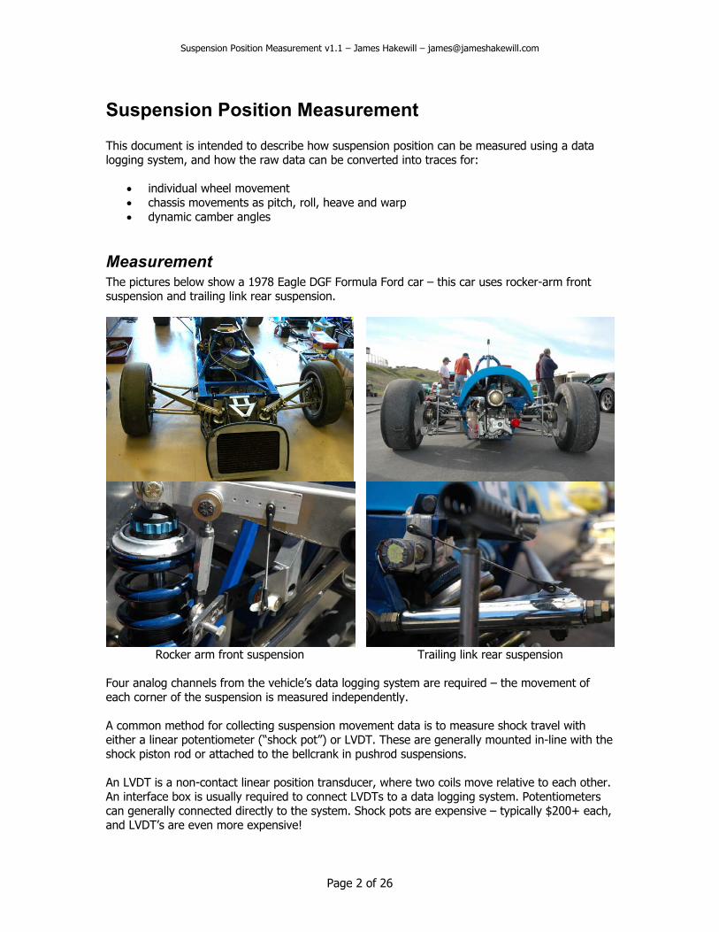
Measurement The pictures below show a 1978 Eagle DGF Formula Ford car – this car uses rocker-arm front suspension and trailing link rear suspension.

Rocker arm front suspension Trailing link rear suspension Four analog channels from the vehicle’s data logging system are required – the movement of each corner of the suspension is measured independently. A common method for collecting suspension movement data is to measure shock travel with either a linear potentiometer (“shock pot”) or LVDT. These are generally mounted in-line with the shock piston rod or attached to the bellcrank in pushrod suspensions. An LVDT is a non-contact linear position transducer, where two coils move relative to each other. An interface box is usually required to connect LVDTs to a data logging system. Potentiometers can generally connected directly to the system. Shock pots are expensive – typically $200+ each, and LVDT’s are even more expensive!

of 26


For the Eagle suspension measurement project, rotary potentiometers (10k linear) from Radio Shack are used, actuated by linkages made from radio-control aircraft hardware. Miniature pushrods and spherical bearings are used for the linkages. The lever arm operating each potentiometer was originally intended as a steering arm for either a boat rudder or an aircraft undercarriage. The advantages and disadvantages of this rotary-pot setup – when compared to motorsport-quality shock pots are as follows:

• Advantages o Cost – excluding the connectors for the data logging box, the total parts bill was

under $30 o No modifications were required to the shocks – all brackets take advantage of

existing suspension bolts and pickups. o The pots can be mounted out of the airflow (and thus away from flying rocks) –

an important consideration on a car with outboard suspension. o It is not necessary to remove the shock pot to change springs

• Disadvantages

o Linkage operating a rotary pot will introduce a small amount of non-linearity into shock travel measurement. This can be factored into the sensor calibration, considered when creating math channels from the raw data, or just ignored.

o Sealed potentiometers should be used for reliability and operation in wet weather – an attempt to seal the pots with duct tape and silicone was made.

o Radio Shack pots are not the highest quality – a long life is not expected Higher quality sealed pots would be a better choice Wire-wound pots should tolerate more cycles before failure, but due to

their construction, do not have the same resolution as a conductive plastic pot

Measurement accuracy The pots are connected as voltage dividers – giving an output between 0v and 5v – proportional to the rotation of the shaft around the 270-degree sweep. In order to limit non-linearity in measurement, the linkages are arranged in order to have the full suspension movement result in a rotation at the pot of around 45-60 degrees. As a result, only a small portion of the total measurement range is being used. We can do a quick calculation to work out the minimum displacement that can be measured. The AIM EVO3 data logging system contains analog-to-digital converters (ADCs) with 12-bit accuracy and input range of 0-5v. An input of 0v corresponds to a raw value of 0, a full-scale input of 5v will result in a full-scale output of 212 –1 = 4095. Thus each output step corresponds to an input change of 5/4096 = 0.00122 volts If we assume a 45-degree movement with a 270-degree pot, the change of output from full droop (0) to full bump (4095) will be: 4096 * 45/270 = 683. If the total wheel movement corresponding to a 45-degree movement at the pot is 5 inches, then the smallest measurement step is 5 / 683 = 0.007” or 0.2mm of wheel movement. For a car with a 57” track, this corresponds to a minimum roll measurement of 0.008 degrees.

of 26


This seems like a reasonable degree of accuracy to get an idea of suspension position around the track. However it would likely not be accurate enough for critical measurements of ride height for optimization of aerodynamic devices such as front wings, splitters or diffusers.

Sample frequency The data to be collected will be used for analysis of roll, pitch and heave – fairly slow-speed changes. As a result, data is collected at 50Hz - a reasonable rate for vehicle parameters. When collecting data for analysis of shock valving, it would typically be necessary to use a much higher sample rate in order to capture high-frequency inputs. It is also likely that a much higher degree of measurement accuracy would also be required.

Sensor calibration The linkages were designed such that the movement of the wheel from full droop to full bump would correspond to 45-60 degrees of movement at the potentiometer. The potentiometer lever-arm positions and pushrod lengths are set so that when the car was at static ride height with driver aboard, the pushrod meets the lever arm at 90 degrees. To calibrate the suspension channels, the following procedure is followed:

• Set all suspension input channels to the logger as 0-100% potentiometers • With the springs and shock bumpstops removed, and roll bars disconnected, calibrate

each channel: • Set 0% = full droop – maximum extension of shock absorber • Set 100% = full bump – maximum compression of shock absorber

A second step is used to get the static ride height information:

• With the springs and bumpstops back in place, • The car is placed on flat and level ground (e.g. scale platform) with the driver aboard • A laptop is connected to the logger and set to display the live suspension position data • The value for each corner at static ride height is noted • This value is used later as a reference value to determine bump and droop

On this type of car, the positions of the shock absorbers at static ride are almost always slightly different from side to side – as a result of the spring seat adjustments required to equalize corner weights. In order to calculate wheel movement, we do of course need to know the relationship between shock movement and wheel position. This will either be represented by constant scaling value or by an equation for rising-rate suspension. It would have been possible to calibrate the sensors for inches or mm of wheel movement (or shock movement) either side of static ride height. The sensor calibration scheme above was chosen to allow for rapid calibration (and recalibration) - without requiring that the calibration step include a measurement of shock position at static ride height. It also allows ride height changes to be made without needing to remove the springs to recalibrate the pots – it is only necessary to note the suspension position values after changing ride height.

of 26


Vehicle data required for basic calculations For the basic calculations of ride height, roll, pitch and heave, we will need:

• Suspension travel at wheel from full droop to full bump – front and rear • Relationship between wheel movement and shock pot movement • Wheelbase • Track – front and rear • Front/rear weight distribution • Reference values for each shock channel at ride height

The table below shows the measurements used for the Eagle Formula Ford. Measurement Front Rear Vertical movement at wheel 127 mm 114 mm Movement at shock (stroke length) 64mm 80 mm ..hence motion ratio 0.5 0.7 Track 1141 mm 1391 mm Wheelbase 2430 mm Front/Rear weight distribution 42% front, 58% rear Rising rate? No - wheel travel and shock travel are linear Shock channel value at ride Note the value reported for each corner

wheel – full droop

wheel – full bump

ground

chassis

motion range at wheel

of 26


Vehicle data required for dynamic camber For dynamic camber calculations, it is necessary to know how camber changes as the wheel moves up and down in roll or bump. This data can be obtained either by direct measurement, or by taking many measurements of suspension components and pickup points, and by using a suspension geometry program such as WinGeo. On the whole, as a wheel moves into bump, the camber becomes more negative – the scheme being to counteract chassis roll during cornering. This is called ‘camber recovery’.

The data used here for the Eagle Formula Ford was measured directly from the vehicle – and the curves are shown in the chart below. Note front and rear static cambers (at zero bump) were set to –1.2 and –0.8 respectively. From the chart it can be seen that the camber curves are indeed curves and not straight lines. A second-order polynomial equation for the curves has been

extracted by using a handy feature of Microsoft Excel. When data is plotted, it is possible to add a “trendline” (linear or polynomial) and display the equation on the chart.

Camber Curves - Eagle DGF Formula Ford

y = -0.0002x2 - 0.0267x - 0.8846

y = -1E-04x2 - 0.0238x - 1.2065-3

-2.5

-2

-1.5

-1

-0.5

0-60 -40 -20 0 20 40 60

Bump (mm)

Cam

ber

(deg

)

Front Rear Poly. (Rear) Poly. (Front)

The equations for camber gain with bump are therefore:

erFstaticambbumpbumpFcamber −−−= 0267.0)*0002.0( 2

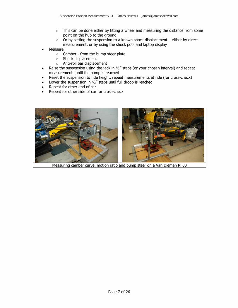
berRstaticcambumpbumpRcamber −−−= 0238.0)0001.0( 2 The camber curves for the Eagle were measured along with the shock and roll bar motion ratios, using the following procedure – very similar to that used to measure bump steer:

• Remove the springs and any shock bumpstops, or remove shock/spring assemblies • Disconnect anti-roll bars • Set the car on a flat and level surface on ride height blocks • Attach bump steer plate (e.g. Longacre 7905) to one corner • Insert steering rack locks to prevent steering whilst the suspension is moved • Set the brakes to prevent rotation of the plate whilst the suspension is moved • Set the suspension at ride height using a jack

of 26


o This can be done either by fitting a wheel and measuring the distance from some point on the hub to the ground

o Or by setting the suspension to a known shock displacement – either by direct measurement, or by using the shock pots and laptop display

• Measure o Camber - from the bump steer plate o Shock displacement o Anti-roll bar displacement

• Raise the suspension using the jack in ½” steps (or your chosen interval) and repeat measurements until full bump is reached

• Reset the suspension to ride height, repeat measurements at ride (for cross-check) • Lower the suspension in ½” steps until full droop is reached • Repeat for other end of car • Repeat for other side of car for cross-check

Measuring camber curve, motion ratio and bump steer on a Van Diemen RF00

of 26


Calculations Now that the car has been measured and the sensors calibrated, it’s time to go out on the track and have some fun – and collect some suspension data while we’re at it.

The picture above shows the Eagle at the apex of turn 9 at Laguna Seca, on the downhill run away from the Corkscrew – as seen from the roll hoop of John Major’s Swift DB6. In the calculations below, the channels are names as follows. Where there are four channels for each corner, only the left-front (LF) channel is shown. It is assumed that the other three corners also exist (RF.., LR.., RR..). Channel Type Description LFshock Measured Left front shock position (0-100%) LFride Constant Left front shock position at ride height (noted during setup) LFmotionratio Constant Left front motion ratio LFshockstroke Constant Left front shock stroke (fully extended to fully closed), in mm LFwheeltravel Constant Left front vertical travel (full droop to full bump), in mm LFstaticcamber Constant Left front static camber at ride height Ftrack Constant Front track in mm Rtrack Constant Rear track in mm Fweight Constant Percentage of weight on front wheels LFbump Math Left front dynamic bump at wheel, either side of ride, in mm LFcamberchange Math Camber change due to bump travel Froll Math Front axle roll (+ve in left hand turn) Rroll Math Rear axle roll Roll Math Roll at CG Pitch Math Pitch angle (+ve when nose-up) Vertical Math Vertical motion of chassis a.k.a heave Fvertical Math Vertical motion of chassis at front Rvertical Math Vertical motion of chassis at rear

of 26


Calculation of shock position Individual shock positions either side of the static ride position are calculated as follows:

• Subtract shock position at static ride from shock position channel, to get movement either side of static ride height, as a percentage of total shock travel

o +ve = bump, -ve = droop

• Multiply by shock stroke (a constant), to get movement at the shock in mm

okeLFshockstrLFrideLFshockpLFshockbum *)( −=

Calculation of wheel position Individual wheel positions either side of the static ride position are calculated as follows:

• Divide shock position in mm by motion ratio to get movement at the wheel in mm o This step would be more complicated with a rising-rate suspension!

tioLFmotionrapLFshockbumLFbump =

It would of course be possible to avoid the step of calculating the shock position in mm – but it may prove useful later – for example to calculate shock piston velocities.

of 26


Calculation of vertical movements By SAE convention, positive vertical movement of the chassis is downwards – the wheels are in bump.

c.g

vertical = 0

vertical > 0 It is useful to calculate vertical mchanges in dynamic ride height. car.

F

R

Vertical movement of the chassis

(Fvevertical =

c.g

ovement of the chassis at each end of the car, to understand Note that this is the change in ride height at the centerline of the

2RFbumpLFbumpvertical +

=

2RRbumpLRbumpvertical +

=

at the center of gravity can be calculated as follows:

2))1(*()* FweightFverticalFweightrtical −+

of 26


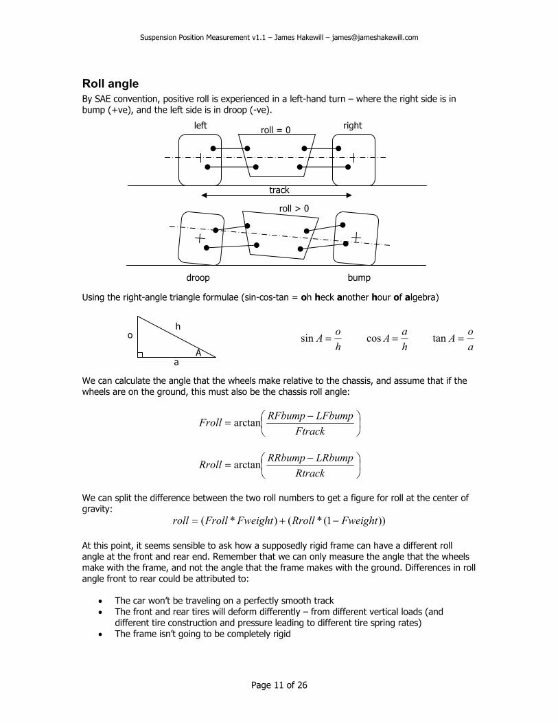
Roll angle By SAE convention, positive roll is experienced in a left-hand turn – where the right side is in bump (+ve), and the left side is in droop (-ve).

roll > 0

track

left roll = 0 right droop bump Using the right-angle triangle formulae (sin-cos-tan = oh heck another hour of algebra)

h

a A

hoA =sin

haA =cos

aoA =tan o

We can calculate the angle that the wheels make relative to the chassis, and assume that if the wheels are on the ground, this must also be the chassis roll angle:

−

=Ftrack

LFbumpRFbumpFroll arctan

−

=Rtrack

LRbumpRRbumpRroll arctan

We can split the difference between the two roll numbers to get a figure for roll at the center of gravity:

))1(*()*( FweightRrollFweightFrollroll −+= At this point, it seems sensible to ask how a supposedly rigid frame can have a different roll angle at the front and rear end. Remember that we can only measure the angle that the wheels make with the frame, and not the angle that the frame makes with the ground. Differences in roll angle front to rear could be attributed to:

• The car won’t be traveling on a perfectly smooth track • The front and rear tires will deform differently – from different vertical loads (and

different tire construction and pressure leading to different tire spring rates) • The frame isn’t going to be completely rigid

of 26


Calculation of pitch angle By SAE convention, positive pitch is a nose-up attitude – with the front end in droop, and the rear end in bump.

pitch = 0

c.g

At each end of the car, we split the difference between the bump travel of the left and right wheel, to get a single number for vertical movement of the wheel pair relative to the chassis at the centerline. The angle made relative to the chassis between the front and rear wheel pairs is taken as the pitch angle. The pitch angle can be calculated as follows:

−

=wheelbase

FverticalRverticalpitch arctan

pitch > 0

c.g

of 26


Dynamic camber angle We can use the combination of wheel movement data, chassis roll and the camber curves to calculate numbers for dynamic camber of each wheel. Using the camber equation and the individual wheel bump data, we can calculate the camber angle that would be measured at the wheel if the chassis were level.

static

For example, using the camber equation for the Eagle’s front suspension, we can work out the camber change due to bump travel:

LFbumpLFbumpangeLFcamberch 0267.0)*0002.0( 2 −−= We actually want to know the dynamic camber relative to the track and not the chassis – so we must factor in the chassis roll number.

dynamic left right

Starting with the static camber at ride height, we calculate dynamic camber as follows. Note that as the camber angles are measured relative to the chassis, we must treat left and right differently. For example, for the front end:

rollangeLFcamberchmberLFstaticcaLFcamber −+=

rollangeRFcamberchmberRFstaticcaRFcamber ++= In the diagram above, the car is making a turn to the left, and thus is experiencing a positive roll angle. The RF wheel has moved into bump, and the suspension will be adding negative camber (RFcamberchange will be negative). The LF wheel is in droop, so LFcamberchange will be positive. The effect of the positive chassis roll is to make the right side camber more positive and the left side more negative.

of 26


AIM math channel definitions The table below shows the settings used to create math channels for the Eagle Formula Ford – using AIM Race Studio Analysis (v2.20.10). Name Units Min Max Equation Note LFshockbump mm -200 200 64*(LFSusp-52)/100 Static ride at 52% position RFshockbump mm -150 250 64*(RFSusp-63)/100 Static ride at 63% position LRshockbump mm -100 300 80*(LRSusp-35)/100 Static ride at 35% position RRshockbump mm -50 350 80*(LRSusp-35)/100 Static ride at 35% position LFbump mm -150 250 LFshockbump/0.5 Front motion ratio 0.5 RFbump mm -50 350 RFshockbump/0.5 Front motion ratio 0.5 LRbump mm -150 250 LRshockbump/0.7 Front motion ratio 0.7 RRbump mm -50 350 RRshockbump/0.7 Front motion ratio 0.7 Fvertical mm -100 100 (LFbump+RFbump)/2 Rvertical mm -100 100 (LRbump+RRbump)/2 vertical mm -100 100 (Fvertical+Rvertical)/2 Froll deg -10 10 atan((RFbump-

LFbump)/1141)/DEG2RAD Front track 1141mm

Rroll deg -10 10 atan((RRbump-LRbump)/1391)/DEG2RAD

Rear track 1391mm

roll deg -10 10 (Froll*0.42)+(Rroll*0.58) Front weight = 42% pitch deg -5 15 atan((Rvertical-

Fvertical)/2430)/DEG2RAD Wheelbase 2430mm

LFcamberchange deg -10 10 (-0.0002*LFbump^2)-

(0.0267*LFbump) See camber curves

RFcamberchange deg -10 10 (-0.0002*RFbump^2)-(0.0267*RFbump)

See camber curves

LRcamberchange deg -10 10 (-0.0001*LRbump^2)-(0.0238*LRbump)

See camber curves

RRcamberchange deg -10 10 (-0.0001*RRbump^2)-(0.0238*RRbump)

See camber curves

LFcamber deg -10 10 -1.6+LFcamberchange-Froll -1.6 static camber RFcamber deg -5 15 -1.6+RFcamberchange+Froll -1.6 static camber LRcamber deg -10 10 -0.8+LRcamberchange-Rroll -0.8 static camber RRcamber deg -5 15 -0.8+RRcamberchange+Rroll -0.8 static camber All channels are sampled at 50Hz.

of 26


Data interpretation There is surely a great deal that can be learned from the suspension data – and a great deal of possible confusion as well. In previous sections we have seen how to calculate a number of useful vehicle parameters. These equations can be used in either a spreadsheet package like Microsoft Excel, or defined as math channels in your favorite data logging analysis package. The data shown here was collected over the course of one three-day weekend at Infineon Raceway (Sears Point) in Sonoma, CA. The top-view map is shown on the left, another map with elevation on the right.

T10 T9 T8/8a

T7T6

T5

T4T3/3a

T1

T2

T11

From the maps it can be seen that Infineon has a variety of different turns and plenty of elevation change. The section from turn 7 through to turn 11 is particularly fun! Before we get into the data analysis, take a moment to compare the basic data logging traces with the maps above.

11 108/8a764 3/3a2

Long

Lat G

Speed

A positive lateral G trace indicates a left turn – negative is a right turn. A positive longitudinal G trace indicates forward acceleration – negative is braking.

of 26


Individual wheel movements The chart below shows an entire lap with the wheel movement (bump) data – relative to static ride height positions. Bump is shown as a positive number, droop as a negative number.

11 10 8/8a764 3/3a 2

RRbump

LRbump

RFbump

LFbump

LongG

LatG

Speed

Apart from expressing sheer horror at the complexity of the chart, we can recognize a number of clear trends in the whole-lap trace:

• During pure cornering (no braking), the left and right traces are not far off being mirror-images

o Take the section between turns 8 and 10 - when turning left, the right wheel moves into bump, the left wheel moves into droop (and vice versa)

• During hard straight-line braking, both front wheels go into bump, and both rear wheels go into droop

o For example the longest braking zone on the track is between turns 10 and 11

• The traces are very noisy o Compared with the lateral and longitudinal G traces, there are lots of tiny spikes

and a number of very big ones.

• And finally - it’s not immediately clear what is happening to the car!

of 26


The segment on the left shows turn 11 in detail. This is a fairly straightforward slow-speed hairpin corner (nearly 180 degrees), which can be split into five sections:

1. Hard straight-line braking starts from high speed.

2. Straight-line braking

3. Turn-in, still on the brakes

4. Cornering, on the throttle

5. Corner exit, on the throttle

We can look at each segment one at a time. Segment 1 and 2 – The LongG trace shows where braking starts. From the wheel traces it can be seen that all four wheels show a large movement in bump immediately prior to braking. This is actually due to a bump in the track – which makes a great braking reference for turn 11. Note that the rear wheels see the bump slightly later than the fronts – we will look athis in more detail later.

t

After braking starts, both front wheels

rebound from the bump but stay much more compressed than before braking began. The gray line for each wheel shows the static ride height position. The rears also rebound, but much more than the fronts, and stay more extended than before braking started. In other words, the nose of the car dives, and the rear comes up. Weight is transferred to the front end.

5 3 4 1 2

11

RRbump

LRbump

RFbump

LFbump

LongG

LatG

Speed

Segment 2 - During the braking zone all four wheels see some up and down movement, but around a stable average. The front end is still compressed, the rear end extended. But – is the up and down movement in the braking zone due to bumps or some kind of oscillation? The longitudinal G trace does not suggest big changes in braking pressure. Looking at the braking zone in detail, we can see that the rear trace (below) is very similar to the front but slightly delayed. The cursor shown is at 11073.9ft, the corresponding peak on the rear trace is at 11081.9ft – suggesting a difference of about 8ft. The accuracy of distance measurements with the logger is not all that great, but each of the other peaks show similar distances of around 8ft. The wheelbase of the car is 2430mm = 95.7”, or 7ft 11.7”. So we can be fairly safe in assume that these are bumps or undulations in the track. By looking at the traces, we can take a guess at which are single-wheel bumps and which affect both sides of the car.

of 26


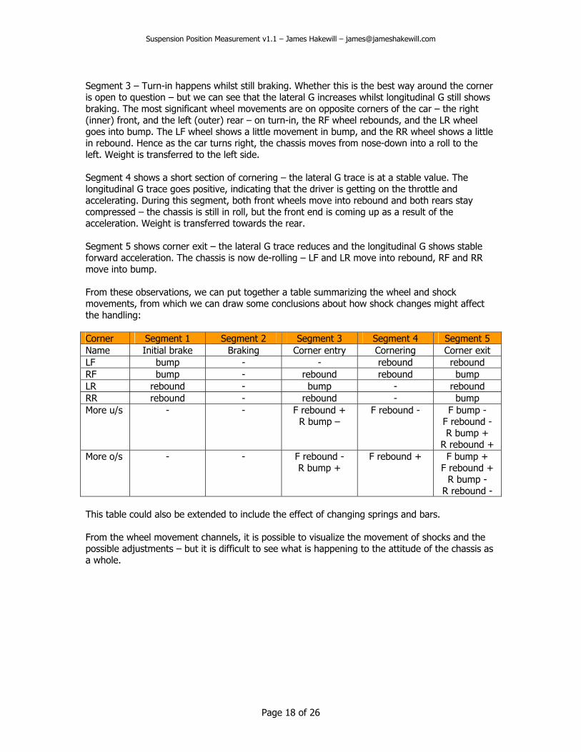
Segment 3 – Turn-in happens whilst still braking. Whether this is the best way around the corner is open to question – but we can see that the lateral G increases whilst longitudinal G still shows braking. The most significant wheel movements are on opposite corners of the car – the right (inner) front, and the left (outer) rear – on turn-in, the RF wheel rebounds, and the LR wheel goes into bump. The LF wheel shows a little movement in bump, and the RR wheel shows a little in rebound. Hence as the car turns right, the chassis moves from nose-down into a roll to the left. Weight is transferred to the left side. Segment 4 shows a short section of cornering – the lateral G trace is at a stable value. The longitudinal G trace goes positive, indicating that the driver is getting on the throttle and accelerating. During this segment, both front wheels move into rebound and both rears stay compressed – the chassis is still in roll, but the front end is coming up as a result of the acceleration. Weight is transferred towards the rear. Segment 5 shows corner exit – the lateral G trace reduces and the longitudinal G shows stable forward acceleration. The chassis is now de-rolling – LF and LR move into rebound, RF and RR move into bump. From these observations, we can put together a table summarizing the wheel and shock movements, from which we can draw some conclusions about how shock changes might affect the handling: Corner Segment 1 Segment 2 Segment 3 Segment 4 Segment 5 Name Initial brake Braking Corner entry Cornering Corner exit LF bump - - rebound rebound RF bump - rebound rebound bump LR rebound - bump - rebound RR rebound - rebound - bump More u/s - - F rebound +

R bump – F rebound - F bump -

F rebound - R bump +

R rebound + More o/s - - F rebound -

R bump + F rebound + F bump +

F rebound + R bump -

R rebound - This table could also be extended to include the effect of changing springs and bars. From the wheel movement channels, it is possible to visualize the movement of shocks and the possible adjustments – but it is difficult to see what is happening to the attitude of the chassis as a whole.

of 26


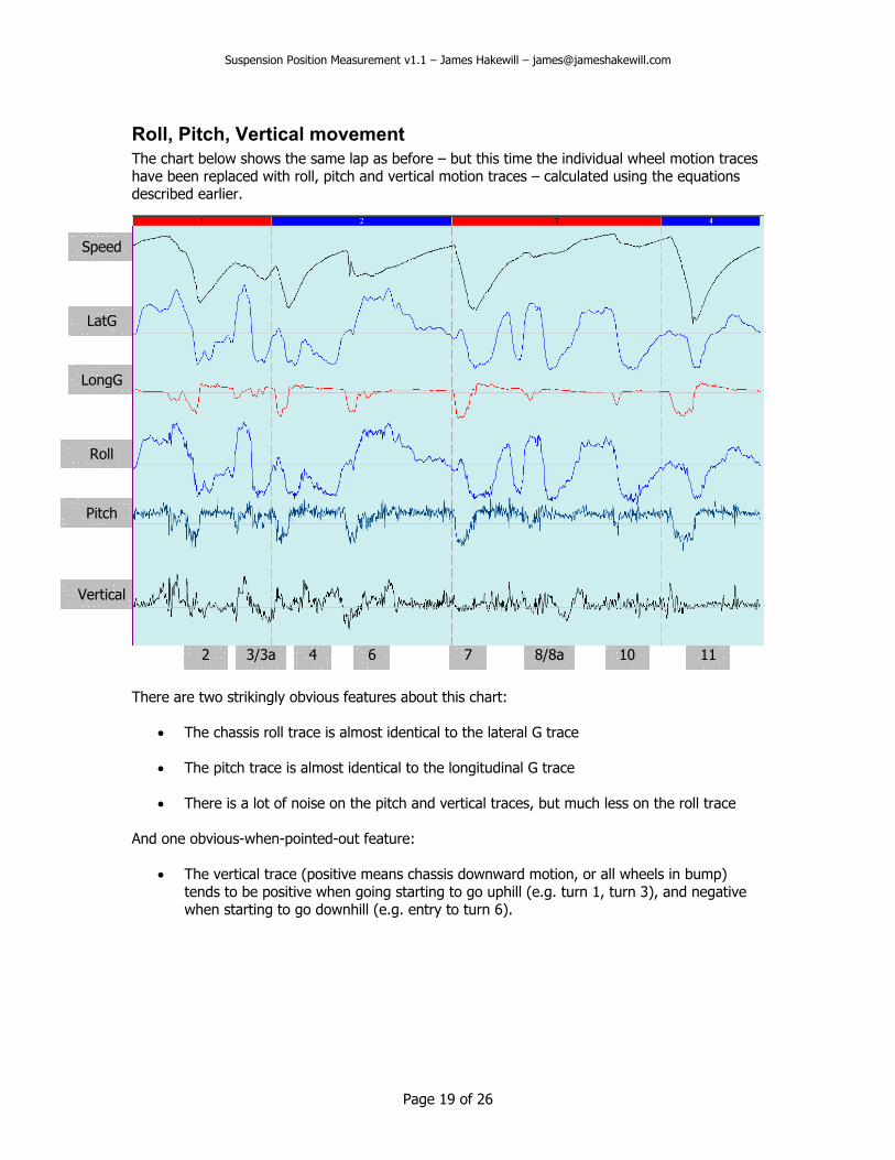
Roll, Pitch, Vertical movement The chart below shows the same lap as before – but this time the individual wheel motion traces have been replaced with roll, pitch and vertical motion traces – calculated using the equations described earlier.

11 10 8/8a764 3/3a 2

Vertical

Pitch

Roll

LongG

LatG

Speed

There are two strikingly obvious features about this chart:

• The chassis roll trace is almost identical to the lateral G trace

• The pitch trace is almost identical to the longitudinal G trace

• There is a lot of noise on the pitch and vertical traces, but much less on the roll trace

And one obvious-when-pointed-out feature:

• The vertical trace (positive means chassis downward motion, or all wheels in bump) tends to be positive when going starting to go uphill (e.g. turn 1, turn 3), and negative when starting to go downhill (e.g. entry to turn 6).

of 26


The segment on the left shows turn 11 in detail once again – but this time using the roll, pitch avertical motion traces. The corner is divided into five sections as before:

nd

1. Hard straight-line braking starts from high

speed.

2. Straight-line braking

3. Turn-in, still on the brakes

4. Cornering, on the throttle

5. Corner exit, on the throttle Once again, we can look at each segment one at a time. Segments 1 and 2 – The LongG trace shows where braking starts. The pitch trace shows immediately that the front end dives – or the rear end rises. The individual wheel motion or Fvertical/Rvertical traces must be consulted to tell which. The vertical trace shows a large movement immediately prior to braking. This is the bump in the track – notice that the vertical trace shows what appears to be up-down oscillation after the big bump during the braking zone. It is not clear from this trace or the wheel traces if this is track

bumps (most likely) or undamped oscillation. There is no significant roll motion.

5 1 2 3 4

11

vertical

pitch

roll

LongG

LatG

Speed

Segment 3 – Turn in. The longitudinal G and pitch traces show that the driver is still on the brakes – the nose is still down as the lateral G and roll increase. Segment 4 – Power application and cornering. As power is applied, we can see that the car goes from nose-down to nose-up very quickly, without any significant change in roll or vertical movement. Segment 5 – Corner exit. As the car exits the corner, pitch and vertical motion remain largely unchanged as the car de-rolls. Notice at the very right hand side of the picture is a large spike on the pitch and vertical traces – this is due to a gearshift. Presumably a faster shift would cause less disruption. From this set of traces it is much easier to visualize the motion of the chassis, and see disruptions on a single channel – however visualizing what is happening for shock adjustments is more difficult.

of 26


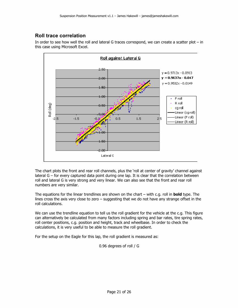
Roll trace correlation In order to see how well the roll and lateral G traces correspond, we can create a scatter plot – in this case using Microsoft Excel.

The chart plots the front and rear roll channels, plus the ‘roll at center of gravity’ channel against lateral G – for every captured data point during one lap. It is clear that the correlation between roll and lateral G is very strong and very linear. We can also see that the front and rear roll numbers are very similar. The equations for the linear trendlines are shown on the chart – with c.g. roll in bold type. The lines cross the axis very close to zero – suggesting that we do not have any strange offset in the roll calculations. We can use the trendline equation to tell us the roll gradient for the vehicle at the c.g. This figure can alternatively be calculated from many factors including spring and bar rates, tire spring rates, roll center positions, c.g. position and height, track and wheelbase. In order to check the calculations, it is very useful to be able to measure the roll gradient. For the setup on the Eagle for this lap, the roll gradient is measured as:

0.96 degrees of roll / G

of 26


Pitch trace correlation The scatter plot below has been arranged to show pitch against longitudinal G – positive LongG represents acceleration and negative LongG is braking. Positive pitch is nose-up. Comparing the pitch trace with longitudinal G does not yield such a clear result as for the roll trace vs lateral G – nevertheless there is still a very strong correlation.

The chart above shows a linear relationship between longitudinal G and pitch. The fact that the chart does not cross the axis at zero (in fact at 0.1466 degrees) suggests that an error has been made in the reference static ride height measurements. Over the wheelbase of 2430mm, 0.1466 degrees corresponds to 6.2mm error. This is entirely possible – the static measurements used in this case were actually taken not from the car on the scales, but from the very end of the ‘in lap’ when the car was seemingly just idling along. There appears to be more noise in the pitch signal than in the roll signal. The pitch angle is calculated from the difference between front and rear vertical movement of the wheels relative to the chassis. The many bumps included in the wheel movement appear to be the cause of noise in the pitch signal – but why does this same noise not appear in the roll signal? Remember that a bump is seen first by the front wheels and then by the rear wheels. A single bump thus produces spikes in the pitch channel first when hit by the front and then by the rear wheels. The noise in the pitch signal caused by the delay between the front and rear wheels hitting two-wheel bumps does appear to be of the right size to account for the spread in the chart above. These bumps also show as noise in the vertical motion trace.

of 26


The standard deviation (aka RMS value) of the ‘pitch error signal’ was calculated – comparing the pitch signal calculation from wheel motion data with the pitch signal calculated using the pitch gradient constant and the LongG signal. A similar calculation was performed for the roll error signal. The results were as follows:

• Standard deviation of pitch error signal = 0.080 degrees -> 3.4 mm over wheelbase

• Standard deviation of roll error signal = 0.065 degrees -> 1.4 mm over average track Since the absolute size of the pitch signal in degrees is much smaller than the roll signal, the spread caused by track imperfections appears larger in the pitch signal.

of 26


Dynamic Camber Another method we can use to get some insight into the behavior of the car is to look at dynamic cambers. Along with vertical load, dynamic camber has an impact on the grip available from each tire. Using the static camber curves described earlier along with the wheel position data, we can calculate the camber gained as a wheel moves into bump, and camber lost as the wheel moves into droop. This can be combined with the chassis roll data to get a figure for dynamic camber. There is one more complicating factor – at the front end of the car, the castor in the front suspension means that dynamic camber changes both with bump/droop and with steering position. This has not been included in the calculations described here! All four analog input channels on the logger system were used for the suspension sensors –

. leaving no free input for the steering channel

itch

ong

akes

Segment 1 – Braking starts. Deceleration begins just after the large bump in the track – visible in earlier examples as a big spike in the vertical trace. Here it shows as all four wheels going into negative camber as they travel into bump. When braking begins, the camber is decreasing on all wheels as they rebound from the bump, but effect of the pchange under braking leaves the front end with increased negative camber. Segment 2 – Straight-line braking. Comparing the traces during this phase to the cambers just before braking begins (very low lateral G, almost zero LG) it can be seen that negative camber has increased at the front and reduced at the rear. Increasing negative camber at the front will have the effect of reducing braking performance as the contact patch must surely be reduced in size. Segment 3 – Turn in on the brakes. As turn-in tplace and roll begins, the negative camber on the loaded left side front and rear wheel is reduced, and negative camber increases on the unloaded right side wheels. Note that at the very end of the sector camber at the LR wheel crosses the zero line and goes positive – which cannot be a good thing. Segment 4 – Power application and cornering. From previous charts we have seen that the pitch

changes as throttle is applied at the start of the segment (following the LongG trace), but the roll angle remains constant. Negative camber is reduced at the front as the nose comes up, but the rear wheels remain at pretty much the same camber angle throughout.

RF camber

RR camber

LF camber

4 5 1 2 3

11

LR camber

LongG

LatG

Speed

Segment 5 – Corner exit. During this phase the car de-rolls whilst pitch remains fairly constantly nose-up. The negative cambers increase on the left side, and reduced on the right side.

of 26


Conclusion This document has shown how useful information about vehicle behavior can be extracted from suspension position measurements – even when those measurements are made with a low-cost 4-channel data logger and very low cost measurement hardware. Note that no information has been presented regarding shock speeds and shock histograms – this may be covered in a future document. Once the vehicle data has been extracted, how it is used to improve vehicle or driver performance is yet another world of mystery – but to make good decisions you need good information.

of 26


of 26

Document information Title Suspension Position Measurement Author James Hakewill Last Saved 11/03/2005 2:07 PM by James Hakewill

suspension position measurement - james hakewilljameshakewill.com/sus-pos-v1.pdf · shock movement...

Documents