Survey of JPEG compression history analysis

Andrew B. Lewis

Computer Laboratory

Topics in security – forensic signal analysis

References

I Neelamani et al.:JPEG compression history estimation for color images, IEEETransactions on Image Processing 15(6), 2006

I Hany Farid:Exposing digital forgeries from JPEG ghosts, IEEETransactions on Information Forensics and Security 4(1), 2009

I Andrew B. Lewis, Markus G. Kuhn:Exact JPEG recompression1, to appear in SPIE ElectronicImaging: Visual Information Processing and Communication,2010

1Draft at http://www.cl.cam.ac.uk/~abl26/spie10-recomp-full.pdf

Outline

I Revision of JPEG compression/decompression algorithm

I Probability theory for parameter estimation

I JPEG compression history estimation for color images

I Exact JPEG recompression

The JPEG algorithm

Parameters:

I Quantization: Q L (luma), QC (chroma)

I Sub-sampling: 1× 1 (luma), 2× 2, 2× 2 (chroma)also known as 4:2:0 sub-sampling

I Colour space: Y CbCr

DCT Q L Encode

ImageColourspace

convert

↓ 2×2 DCT QC Encode

↓ 2×2 DCT QC Encode

Y

Cb

Cr

JPEG compression history estimation

I Probabilistically estimate settings used in the previouscompression step

I Input: raw image in colour space F

I Output: compressed representation colour space G ∗,sub-sampling scheme S∗ and quantization tables Q∗

G ∗, S∗,Q∗ = arg maxG ,S ,Q

P(Image,G ,S ,Q)

= arg maxG ,S ,Q

P(Image|G , S ,Q)P(G ,S ,Q)

Terminology of inverse probability

Unknown parameters θ, data D, assumptions H

P(θ|D,H) =P(D|θ,H)P(θ|H)

P(D|H)

posterior =likelihood× prior

evidence

The quantity of P(D|θ,H) is a function of both D and θ. Forfixed θ it defines a probability over D. For fixed D it defines thelikelihood of θ.2

2More in David J. C. MacKay: Information Theory, Inference and LearningAlgorithms, Cambridge University Press.

Maximum a posteriori estimation

We wish to estimate θ on the basis of data D. The maximumlikelihood (ML) estimate of the parameters from the data is

θML(D) = arg maxθ

P(D|θ)

and maximum a posteriori (MAP) estimate is

θMAP(D) = arg maxθ

P(D|θ)P(θ)

Expectation maximization

ML estimate requires the marginal likelihood, if we have hiddenvariables.

θML(D) = arg maxθ

P(D|θ)

P(D|θ) =∑Z

P(D|z ,θ)P(z |θ)

Evaluating the sum is sometimes computationally infeasible. Theexpectation-maximization algorithm can be used instead.

Expectation: Q(θ|θ(t)) = EZ |x ,θ(t) [log L(θ; x ,Z )]

Maximization: θt+1 = arg maxθ

Q(θ|θ(t))

No guarantees of convergence

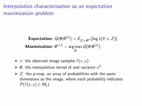
Interpolation characterisation as an expectationmaximization problem

Expectation: Q(θ|θ(t)) = EZ |x ,θ(t) [log L(θ; x ,Z )]

Maximization: θt+1 = arg maxθ

Q(θ|θ(t))

I x : the observed image samples f (x , y)

I θ: the interpolation kernel ~α and variance σ2

I Z : the p-map, an array of probabilities with the samedimensions as the image, where each probability indicatesP(f (x , y) ∈ M1)

Compression history estimation as MAP problem

θMAP(D) = arg max

θ

P( D | θ )P( θ )

G ∗,S∗,Q∗ = arg max

G , S ,Q

P( Image | G , S ,Q )P( G , S ,Q )

Estimating quantization tables Q∗ (1)

I Small set of possible values for G and S .

I C’space to G ∗, sub-sample with S∗, then forward DCT gives anear-periodic distribution of coefficients ΩG ,S over image.

I G , S , Q and XG ,S ∈ ΩG ,S independent

G ∗,S∗,Q∗ = arg maxG ,S ,Q

P(ΩG ,S |G ,S ,Q)P(G )P(S)P(Q)

G ∗,S∗,Q∗ = arg maxG ,S ,Q

∏eXG ,S∈ΩG ,S

P(XG ,S |G ,S ,Q)P(G )P(S)P(Q)

Estimating quantization tables Q∗ (2)Since the decompressor’s dequantization,

I DCT coefficients Xq were IDCT’ed;

I the results were up-sampled if necessary; and

I the image was converted to the RGB colour space.

I We received the image, and applied a forward colour space conversion;

I we downsampled the planes, if appropriate; and

I we applied the forward DCT to get eX .

Rounding errors accumulate during every stage of this process.Therefore, we model the DCT coefficient values

X = Xq + Γ

where original DCT coefficients Xq are modelled by a sampled

zero-mean Laplace distribution x

P(x)

and rounding error Γ is

drawn from a truncated normal distribution x

P(x)

.

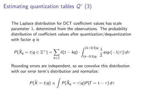
Estimating quantization tables Q∗ (3)

The Laplace distribution for DCT coefficient values has scaleparameter λ, determined from the observations. The probabilitydistribution of coefficient values after quantization/dequantizationwith factor q is

P(Xq = t|q ∈ Z+) =∑k∈Z

δ(t − kq) ·∫ (k+0.5)q

(k−0.5)q

λ

2exp (−λ|τ |) dτ

Rounding errors are independent, so we convolve this distributionwith our error term’s distribution and normalize:

P(X = t|q) ∝∫

P(Xq = τ |q)P(Γ = t − τ) dτ

Estimating quantization tables Q∗ (4)

If we assume a uniform prior P(q) for quantization factors, we cannow find the most likely value for a particular quantization factorq = Q∗i ,j by maximizing P(X |q). This is repeated for eachquantization factor Q∗i ,j for (i , j) ∈ (0, 0), . . . , (7, 7):

q∗ = arg maxq∈Z+

∏eX∈Ω

P(X |q)

Evaluation

I Allows for arbitrary colour space conversion, sub-sampling andquantization table parameters

I Not implementation specific

I Partially recovered quantization tables could be used todetermine quality factorQuality factors q ∈ 1, . . . , 100 map onto quantization tables in many

compressor implementations

I Statistical rather than exact

I Can’t recover bitstream

I Tikhonov deconvolution filter introduces errors

I Errors in the quantization table when most DCT coefficientsat a particular frequency are zero

I No data for the quantization table when all are zero (lowquality factors)

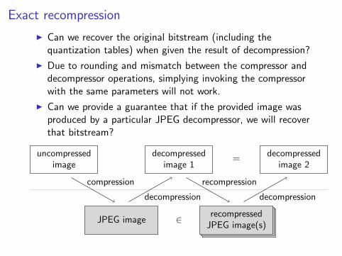
Exact recompression

I Can we recover the original bitstream (including thequantization tables) when given the result of decompression?

I Due to rounding and mismatch between the compressor anddecompressor operations, simplying invoking the compressorwith the same parameters will not work.

I Can we provide a guarantee that if the provided image wasproduced by a particular JPEG decompressor, we will recoverthat bitstream?

uncompressedimage

decompressedimage 1

=decompressed

image 2

JPEG image ∈ recompressedJPEG image(s)

compression

decompression

recompression

decompression

Applications of exact recompression

I The input to JPEG compressors is often previouslycompressed image data. Detecting this and recompressingexactly will reduce the information loss from recompression.

I Hinder forensic analysis – double compression detection, JPEG‘ghosts’, . . .

I Detect tampered regions in an uncompressed image, when thebackground was output by a JPEG decompressor

I Some copy-protection schemes rely on the fact that copies willbe recompressed, lowering the quality.

Information loss in the decompressor

I Model sources of uncertainty (rounding, range limiting) wheninverting operations in the decompressor using intervals ofintegers. We store intervals for all intermediate values in thedecompressor.

I Because we are modelling the exact computations, exactrecompressors are implementation-specific.

Chroma down-sampling example (1)

IJG chroma upsampling filter weights contributions from neighbouringsamples by 1

16 (1, 3, 3, 9) in order of increasing proximity.

×3 ×1

×9 ×3 ×3

×1

×9

×3

×3×1

×9×3 ×3

×1

×9

×3

vx,y =

⌊1

16(8 + α · wi−1,j−1 + β · wi,j−1 + γ · wi−1,j + δ · wi,j)

⌋,

with weights

(α, β, γ, δ) =

(1, 3, 3, 9) x = 2i , y = 2j

(3, 1, 9, 3) x = 2i − 1, y = 2j

(3, 9, 1, 3) x = 2i , y = 2j − 1

(9, 3, 3, 1) x = 2i − 1, y = 2j − 1.

Chroma down-sampling example (2)

We need to solve for the down-sampled weights wi ,j :

vx ,y =

⌊1

16(8 + α · wi−1,j−1 + β · wi ,j−1 + γ · wi−1,j + δ · wi ,j)

⌋Interval arithmetic rules give

wi ,j =

[⌈1

δ(vx ,y ⊥ × 16− (8 + α · wi−1,j−1 + β · wi ,j−1 + γ · wi−1,j))

⌉,⌊

1

δ(vx ,y > × 16 + 15− (α · wi−1,j−1 + β · wi ,j−1 + γ · wi−1,j))

⌋]

Chroma down-sampling example (3)

k ← 0w0

x ,y ← [0, 255] at all positions −1 ≤ x ≤ w2 ,−1 ≤ y ≤ h

2repeat

k ← k + 1change scan order of (x , y) ( , , , )for each sample position (x , y) in the upsampled plane do

for (i ′, j ′) ∈ (i − 1, j − 1), (i , j − 1), (i − 1, j), (i , j) dow ′i ′,j ′ ←

⋃s∈v c

x,ya :

Equation satisfied with a for wi ′,j ′ , s for vx ,y

and current estimates wx ,y for other w values.

wki ′,j ′ ← wk−1

i ′,j ′ ∩ w ′i ′,j ′end for

end foruntil wk = wk−1

w cx ,y ← wk

Performance

4050

6070

8090 0

0.10.2

0.30.4

0.5

IJG quality factorinfeasible blocks

total blocks

Number of testimages

Figure: Recompression performance for a dataset of uncompressedimages from the UCID. 1338 colour images were compressed anddecompressed at quality factors q ∈ 40, 60, 70, 80, 82, 84, 86, 88, 90,then recompressed. The proportion of blocks at each quality factor whichwere not possible to recompress due to an infeasible search size is shown.