survey in lake ... · pdf filethe navigation data was displayed in real time using the...

Geofísica Internacional

ISSN: 0016-7169

[email protected]

Universidad Nacional Autónoma de México

México

Galindo Domínguez, Roberto E.; Bandy, William L.; Mortera Gutiérrez, Carlos A.; Ortega Ramírez,

José

Geophysical-Archaeological Survey in Lake Tequesquitengo, Morelos, Mexico

Geofísica Internacional, vol. 52, núm. 3, 2013, pp. 261-275

Universidad Nacional Autónoma de México

Distrito Federal, México

Available in: http://www.redalyc.org/articulo.oa?id=56827417005

How to cite

Complete issue

More information about this article

Journal's homepage in redalyc.org

Scientific Information System

Network of Scientific Journals from Latin America, the Caribbean, Spain and Portugal

Non-profit academic project, developed under the open access initiative

http://www.redalyc.org/revista.oa?id=568

http://www.redalyc.org/articulo.oa?id=56827417005

http://www.redalyc.org/comocitar.oa?id=56827417005

http://www.redalyc.org/fasciculo.oa?id=568&numero=27417

http://www.redalyc.org/articulo.oa?id=56827417005

http://www.redalyc.org/revista.oa?id=568

http://www.redalyc.org

Geofísica Internacional (2013) 52-3: 261-275

Resumen

En agosto del 2009 se llevó a cabo una prospección geofísica subacuática con fines arqueológicos en el Lago de Tequesquitengo, en el Estado de Morelos. El objetivo del trabajo fue localizar y delimitar los restos del pueblo que yace sumergido en el fondo del lago desde mediados del siglo XIX. Se realizó la adquisición y mapeo de datos magnéticos, batimétricos de ecosondeo monohaz y se obtuvieron imágenes de sonar de barrido lateral de 200 KHz. Para el posicionamiento de la embarcación durante la prospección se empleó un sistema de navegación marina GPS. A excepción de los restos de las estructuras culturales más grandes visibles en las imágenes de sonar, los resultados magnéticos fueron más útiles para delimitar la extensión del pueblo sumergido. Los datos muestran anomalías con longitud de onda corta alrededor y en las inmediaciones de la iglesia sumergida. Asimismo, las anomalías con los componentes de longitud de onda en la banda más corta están agrupadas en el área adyacente inmediata al este de la iglesia. Los componentes de longitud de onda corta sólo se observan alrededor de la iglesia y no en el resto del área prospectada, por lo que proponemos que éstos corresponden a restos culturales pertenecientes al pueblo sumergido.

Palabras clave: Lago de Tequesquitengo, México, Geofísica, Arqueología, Magnética.

Abstract

In August 2009, a marine geophysical survey was conducted in Lake Tequesquitengo (located in the state of Morelos, Mexico) to delineate the extent of the remains of a small town that has been submerged since the mid 19th century. The survey consists of the acquisition and mapping of magnetic, single beam bathymetric and side-scan sonar data. A dual receiver marine GPS navigation system was used to position the boat during the survey. Except for the larger structural remains that are visible on the side scan sonar images, the magnetic anomaly map proved to be most useful in delineating the extent of the town. These anomalies exhibit short wavelength components in the area surrounding a submerged church, with the shortest wavelength components being confined to the area immediately east of the church. These short wavelength components are only observed near the church; therefore, we propose that they delineate the buried remnants of the submerged town.

Key words: Lake Tequesquitengo, Mexico, Geophysics, Archaeology, Magnetic.

261

Geophysical-Archaeological Survey in Lake Tequesquitengo, Morelos, Mexico

Roberto E. Galindo Domínguez*, William L. Bandy, Carlos A. Mortera Gutiérrez and José Ortega Ramírez

Received: September 7, 2012; accepted: February 25, 2013; published on line: June 28, 2013

R. E. Galindo Domínguez*

W. L. BandyC. A. Mortera GutiérrezInstituto de Geofísica, Universidad Nacional Autónoma de México, Ciudad UniversitariaDelegación Coyoacan, 04510México D.F., México*Corresponding author: [email protected] J.Ortega RamírezGeophysics LaboratoryInstituto Nacional de Antropología e HistoriaMéxico D.F., México

Original paper

R. E. Galindo Domínguez, et al.

262 Volume 52 Number 3

Introduction

Marine geophysical techniques are useful to locate and map archaeological sites submerged in lakes (e.g. Cassavoy and Crisman, 1988; Crisman, 2005). However, few such studies have been attempted in Mexican lakes, many of which may contain significant archaeological remains and artifacts. In August 2009, the first marine geophysical-archaeological survey within Lake Tequesquitengo, located in Morelos, Mexico (Figure 1), was undertaken by students and investigators from the Instituto de Geofisica, UNAM. Since the middle part of the 19th century, a small colonial-style town has been submerged in the southernmost part of this lake where the church tower and some of its walls and columns are still observed. These structures have been previously mapped; however, the full extent of the town has yet to be determined. The purpose of the study is to define using geophysical methods (total field magnetic, bathymetry, and side scan sonar) the extent of the submerged town. The results should prove useful for planning future archaeological dives in this area.

Preliminary results of this work have been presented in Galindo et al. (2009), Galindo (2012) and in the thesis of Galindo (2011). Herein we present these results in a more concise, readily available form along with previously unpublished results of an analysis of the spatial wavelength components of the magnetic anomalies.

Previous Work

The most prominent cultural remains are associated with a submerged church located within the southernmost part of Lake Tequesquitengo (Figure 2). The church lies on a small bathymetric high at about 2057160m N, 471940m E (UTM zone 14Q): which is the position of the navigation buoy marking the bell tower as determined using a single frequency GPS. With the exception of equipment testing, no detailed geophysical survey has been previously conducted in the lake. However, two separate groups have conducted professional underwater archaeological surveys (dive surveys) in the area around the church. In the latter part of 1987, the PROTEO group (Lowenstein et al., 1991) began a 5-year, systematic survey (“Proyecto Pueblo Hundido de Tequesquitengo”) of the area around the submerged church. They found a major concentration of cultural remains located in a 20m x 20m area (400 m2 area) corresponding to the remains of the church (the bell tower, walls, columns, etc.). They also report a second area of cultural remains, which they called “La Casa del Cura” (possibly the remains of the Presbytery), located 15 meters north of the bell tower, which covers an area of about 200 m2. The plan, constructed by the PROTEO group, of the structures found in the area of the church tower and their relation with the Presbytery is presented in Figure 3a. The area encompassing both structures is roughly 55m in the N-S direction by 45 m in the E-W direction (Figure 3b).

The second group of investigators, headed by Biologist Virginia Urbieta, extended the search area of the PROTEO group (Figure 4). They found cultural remains (e.g., columns, remains of walls and a small shelter, etc.) in the area surrounding the sites mapped by PROTEO. Specifically, remains were mapped up to 30 meters north of the Presbytery and up to 30 meters south and west of the bell tower. Thus, the results of the archaeological dives have established that cultural remains exist for a distance of at least 60 meters north of the bell tower, 40 meters south of the bell tower, 40 meters west of the bell tower, and 15 meters east of the bell tower: an area of about 5,500 m2. Of importance to our study is that Urbieta´s group detected the upper parts of some buried structures east and NE of the church; thus, it is quite possible that the remains extend farther from the mapped area, especially in the deeper parts of the lake located to the east and northeast of the church where artifacts may be completely covered by sediments.Figure 1. Location of Lake Tequesquitengo south of

Cuernavaca and the Teoloyucan Magnetic Observatory located in the NW corner of Mexico D.F. (Background

map from Google Earth).


July - September 2013 263

Figure 2. Location map of the survey area and submerged church (Background map from

Google Earth).

Figure 3. Archaeological site plans illustrating the relative positions of the major structural remains. A) San Juan Bautista Church as mapped during the PROTEO surveys (Lowenstein et al., 1991). B) Church

and Presbytery.



Figure 4. Map of the church and surrounding areas as determined by the group headed by Virginia Urbieta (unpublished map graciously provided by Virginia Urbieta).



Geophysical Survey

The main survey covered an area of 284,640 m2

in the southernmost part of the lake (Figure 2). Total field magnetic measurements, bathymetry, side scan sonar data collected along 36 parallel lines oriented at an azimuth of 339° were used in the present analysis (Figure 5). The profiles have an average length of 593 meters with a planned line spacing of 15 meters.

The boat used in the survey was the “Barracuda” (Figure 6) which was graciously provided by the port captain of Tequesquitengo. The position of the ship during the survey was determined using the Kongsberg SEAPATH20 dual GPS receiver, marine navigation system which provides the boats heading, position and speed. The navigation data was displayed in real time using the Nobeltec navigation program which was used by the captain as a helmsman’s display, which helps the captain to keep the boat on the survey line.

The total field magnetic data was collected using the Geometrics Model G877 marine proton procession magnetometer, which has a resolution of 0.1 nT (Breiner, 1973). The sensor, which is connected to the recording computer by an electrical/strength cable, was towed a distance of 50 meters behind the boat

to minimize the magnetic noise generated by the boat and its’ motor. Non-metal floats were mounted to the cable to keep the sensor at a depth of 1 meter so that the cable and sensor would not hit the lake bottom during turns nor snag on submerged objects. The magnetic data was recorded at a sampling rate of 2 seconds using the Geometrics Mag Log Lite program. This program also calculates and records the position of the magnetic sensor using the Ship´s navigation data. Magnetic data was not recorded

Figure 5. Survey lines superimposed on the magnetic contour map (black-shaded contours) and bathymetric contours (white contours) constructed from the data collected during the survey.

Figure 6. Photo of the “Barracuda” taken during installation of the equipment.



while the boat was turning to the next line. During the survey, the DST (Disturbance Storm Time) index data from the Kyoto observatory, Japan, was periodically checked to make sure that no magnetic storm was occurring during data acquisition. The plot (Figure 7) of the DST index for August 26 and 27, 2009 illustrates that the data collected during our survey were not perturbed by any magnetic storms.

Bathymetric data and side scan sonar data

was obtained using the Konsgberg EA 600 (Konsgberg, 2004, 2007) combination single beam echo-sounder and side-scan sonar system. The frequency of the two side-scan transducers is 200 KHz (Figure 8). The transducer for the echo-sounder can be driven at either 38 or 200 KHz; during the survey the 200 KHz option was used.

Total Field Magnetic Data Processing

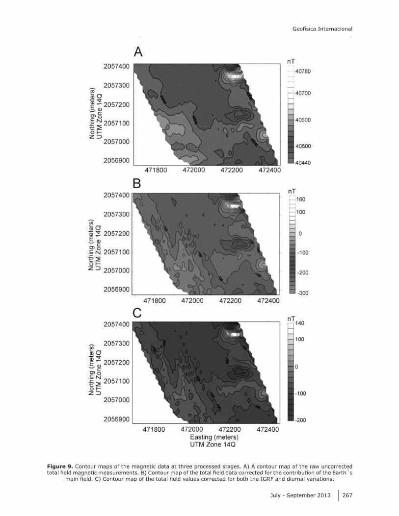
A contour map of the raw uncorrected total field magnetic measurements of the survey is presented in Figure 9a. In addition to the

magnetic field produced by the cultural artifacts of the town (which is what we are interested in), the raw data measured by the proton precession magnetometer includes a component due to the Earth´s main field, a component due to the Sun which causes fluctuations (diurnal variations) in the Earth´s magnetic field by inducing currents in the ionosphere (Otaola, et al., 1993; Blakely, 1996), a component due to the ships’ heading (or sensor orientation), and a component due to other ship effects (which we assume to be small as the sensor was towed 50 meters behind the boat). Thus, to determine the magnetic field produced by the cultural artifacts, we must first remove all the other components as best we can, or in other words, we must reduce the measured values to magnetic anomalies.

Removal of the Earth´s main field (IGRF)

The first step in the reduction of the raw data is to remove the contribution of the Earth´s main field. This is accomplished by estimating the value of the Earth´s main field at the location and time of each measurement using model 11 (IAGA, Working Group V-MOD, 2010) of International Geomagnetic Reference Field (IGFR11) and removing this value from the measured value. The Fortran source code of the IGRF11 subroutine was obtained from http://www.ngdc.noaa.gov/IAGA/vmod/igrf.html. A main driver was written to adapt the subroutine for use in reducing marine data. Figure 9b presents a contour map of the total field data corrected for the contribution of the Earth´s main field.

Correction for Diurnal Variations

The next step in the reduction procedure is to remove the diurnal variations from the IGRF-corrected values. To accomplish this, the total field magnetic data for the survey dates were obtained from the magnetic observatory at Teoloyucan (a permanent magnetic observatory maintained by the Instituto de Geofísica, UNAM)

Figure 7. Graph of the equatorial DST Index verses time (GMT) for August 2009. Data obtained from the Kyoto Observatory [http://swdcwww.kugi.kyoto-u.ac.jp/dstdir/index.html].

Figure 8. Photographs of the survey equipment. Left side, EA600 echosounder transducer. Right side,

Sidescan sonar transducers.



Figure 9. Contour maps of the magnetic data at three processed stages. A) A contour map of the raw uncorrected total field magnetic measurements. B) Contour map of the total field data corrected for the contribution of the Earth´s

main field. C) Contour map of the total field values corrected for both the IGRF and diurnal variations.



which is located at 19° 44’ 45.100”N, 99° 11’ 35.735”W, 125 km from Lake Tequesquitengo (Figure 1). These data were corrected for the IGRF again using the IGRF11 model for the Earth´s main field and the high frequency components of the Teoloyucan data were removed by fitting a polynomial (magnetic value as a function of time) to the data. The resulting values are assumed to represent the low frequency diurnal variations at the survey area. Each measured value was then corrected using the polynomial value corresponding to the time of the measurement. A contour map of the total field values corrected for both the IGRF and diurnal variations is presented in Figure 9c.

Correction for Ship´s Heading

The procedure used herein to make the heading corrections is based on the mis-tie correction algorithm of Bandy et al. (1990), modified so that it could be applied to grids (Bandy et al., manuscript in preparation). The procedure is as follows. The survey is separated into two groups of lines, all lines in each group having roughly the same overall heading, and hence the same heading error. The two data groups

are gridded separately using the exact same grid specifications for both grids, and the mean difference between the two grids is determined. The heading corrections are then applied by adding one half of the mean difference to the data of one of the group and subtracting one half of the mean difference from the data of the other group (similar to equations 15a and 15b of Bandy et al., 1990). The corrected data of the 2 groups are then re-combined and the entire data set is gridded. A contour map of the final magnetic anomalies (i.e. after correcting the raw data for the Earth´s main field, diurnal fluctuations and ship´s heading) is presented in Figure 10. The area marked by the rectangle is the area where the principle cultural remains, such as the church, have been found and mapped during previous dive surveys. The area enclosed by the circle is interpreted from the magnetic characteristics to be the area most likely to contain additional cultural artifacts. It is interesting to note (Figures 9 and 10) that the magnetic signature of this zone has been progressively clarified at each step of the reduction of the raw data to anomaly values as is expected if the signature is due to real sources.

Figure 10. Contour map of the final magnetic anomalies (i.e. after correcting the raw data for the Earth´s main field, diurnal fluctuations and ship´s heading). The rectangle delineates the area mapped by previous dive surveys. The

area enclosed by the dashed circle is the area that we propose to contain cultural remains.



Fig

ure

11

. Fi

lter

pane

ls o

f th

e re

sults

of

the

appl

icat

ion

of e

ight

diff

eren

t ban

d pa

ss fi

lter

s to

the

mag

netic

anom

aly

map

illu

stra

ted

in F

igur

e 10

. The

firs

t of

th

e tw

o nu

mbe

rs a

t the

top

of e

ach

pane

l is

the

sho

rtes

t w

avel

engt

h (i

n m

eter

s)

pres

ent in

the

pan

el.

The

seco

nd o

f the

tw

o nu

mbe

rs a

t th

e to

p of

eac

h pa

nel

is t

he l

onge

st w

avel

engt

h (i

n m

eter

s)

pres

ent

in t

he p

anel

. Fo

r re

fere

nce,

the

lo

catio

n of

the

chu

rch

tow

er (

4719

40m

E,

205

7160

m N

) is

mar

ked

by th

e sm

all,

blac

k sq

uare

s. T

he th

ree

mag

netic

zon

es

surr

ound

ing

the

chur

ch a

re il

lust

rate

d in

pa

nel I

I. S

ee t

ext

for

mor

e de

tails

.



Figure 12. Newly constructed bathymetric map of the survey area. A) Contour representation. B) 3-D surface representation. Note the small high to the west where the remains of the church are located.



Frequency Filtering

Wavelength filtering was applied to the gridded data which was used to produce the map shown in Figure 10 to better isolate those anomalies associated with the remains of the town. The spacing between grid nodes was in all cases 15 meters to coincide with the spacing between survey lines. Thus, the minimum resolvable component wavelength is 30 meters. Filtering was accomplished using the program FFTFIL which is included in the Potential-Field geophysical software version 2.0 obtained from the United States Geological Survey (Hildenbrand, 1983; Cordell et al., 1992).

Figure 11 illustrates the application of eight different trapezoidal, band pass filters. The two numbers at the top of each panel are the limits of the wavelengths which are entirely removed by the filter. In all filters, a 5 meter linear ramp has been applied at each end of the filter. Thus, for example, in the filter used to produce Panel IV wavelengths between 40 and 45 meters were passed with no reduction of amplitude, and frequencies less than 35 meters and greater than 50 meters were completely removed. Also shown in the panels is the location of the church tower (filled square) for reference.

Bathymetry and side scan sonar images of the site

Single beam echo-sounder bathymetric data and side scan sonar images were collected concurrent with the magnetic data using the Kongsberg EA-600 echo sounder including its side scan option. The bathymetric contour map and surface relief illustration of these data are presented in Figures 12a and 12b, respectively. Water depths range from 10 meters in the eastern and western margins of the southern part of the survey area to 18.5 meters to the north. A small bathymetric high (values reaching up to -13m) is present between the -13.5m and -14m contours in the left-central part of the map, with the bathymetric expression of the church easily noted at UTM 2057160m N, 471940m E. The bell tower of the church and several other large structures are also clearly imaged on the bathymetry and sidescan records (Figure 13). The sidescan images were featureless in the deeper parts (>10 m) of the survey area, even in areas where we knew that a 50 gallon barrel was present on the lake floor. This result is puzzling as the sidescan images in the shallow water areas clearly imaged channel cuts and differences in reflectivity of the lake floor. Given the good images of the lake floor in shallow water and the good images of the bell tower, we conclude that the system was working and we suspect that the poor images in deeper

water may be due to a strong stratification of the water column which prevented the sound from reaching the bottom. Alternatively, there may be a thick layer of mud or suspended sediments in the deeper parts of the lake which, given the high frequency (200 kHz) of the sidescan transducers, may be masking the barrel and other objects on the lake floor.

Results and Discussion

The major cultural remains (church, Presbytery and the remains located north of the Presbytery) determined by the previous dive surveys covers an area of about 65 m in the north-south direction and 20 meters in the east-west direction, a total

Figure 13. EA600 bathymetry profile (top) and associated side-scan sonar image (bottom) of the remains of the church. Note: the church tower on both profiles is aligned. The church tower is the highest structure extending from the lake floor on the left side

of both images.



area of 1300 m2. To compare the magnetic anomalies with the cultural remains, this area is superimposed on the bathymetry and magnetic anomaly contours (Figure 14). Most notable is that the magnetic anomalies are markedly different in the area immediately north and east of the church, towards the deeper part of the survey area, than those observed in the rest of the survey area. Specifically, in the area immediately north and east of the church, the anomaly pattern consists of low-amplitude, short-period anomalies forming a “checkerboard” pattern. In marked contrast, no short period anomalies are observed in the eastern half of the survey area farther away from the church. Instead, that area contains only a few, very high amplitude (-180 to 160 nT), longer wavelength anomalies. [Concerning the very high amplitude anomaly located in the NE corner of the survey, given its very large amplitude and its location adjacent to a hotel that was in the process of being renovated at the time that the survey was conducted, we conclude that this anomaly most likely is not associated with artifacts of the submerged town. Consequently, this anomaly is not considered further in this paper.] South of the church some low amplitude, short period anomaly are observed but they do not form a checkerboard pattern. Immediately west of the church no short period anomalies

are observed. This spatial distribution of the magnetic anomalies suggests that the remains of the settlement were confined mainly to the area east of the church where the checkerboard pattern of anomalies is observed.

The above inference that the remains of the town are confined to the area east of the church is somewhat unexpected as settlements of this period commonly surrounded the church. To check the validity of this inference, the magnetic anomaly map was band pass filtered at eight different frequency bands (Figure 11). Based on the spatial distribution of the various wavelength components (and their amplitudes) comprising the magnetic anomalies, we delineate three distinct zones in the vicinity of the church. These zones are outlined in Panel II of Figure 11.

The first zone, Zone 1, corresponds to the area of the “checkerboard” magnetic anomaly pattern. It is best defined in Panel I, although the anomalies in Zone 1 have wavelength components in the 30 to 45 meter band (Panels I, II and III). Panel I indicates that the church is located on the western margin of this zone and that the zone extends approximately 120 meters east of the church, and roughly 70 meters north and south of the latitude of the church. Thus, this

Figure 14. Filled magnetic contour map with bathymetric contours (white lines) superimposed. Small black box is the area (20m x 20m) of the remains of the church. Red box (45m x 20m) is the area of the remains of the Presbytery and the remains just to the north mapped by Virginia Urbieta. Big yellow box is the over-all area mapped during the

two dive surveys.



zone covers an area of roughly 16,800 m2. The amplitudes of the wavelength components in this zone are the highest of the three zones, so much so that these anomalies are readily apparent on the unfiltered data (Figure 10). Amplitudes within the 20 to 35m, 25 to 40m and 30 to 45m band are -15 to 10nT, -20 to 15 nT and -10 to 5 nT, respectively. It is clear that these short wavelengths appear nowhere else in the survey area except in the area adjacent to the church. This strongly suggests that these anomalies can be attributed to the remains of the town.

The second zone, Zone 2, lies northwest of the church. Here, the component wavelengths of the anomalies are somewhat longer at the low end of the spectrum than those of Zone 1, lying in the 35 and 45 meter band (Panels II and III). Zone 2 also differs from Zone 1 in that the amplitudes of the wavelength components are less. Specifically, within the 25 to 40m and 30 to 45m bands the observed amplitudes are -10 to 10nT and -5 to 5nT, respectively. There is also a smaller area much further to the south at 2057000m N, 471900m E which exhibits similar component wavelengths, but with very low amplitudes (-5 to 5nT).

The third zone, Zone 3, is located immediately SW of the church. Here, the component wavelengths are significantly longer, lying in the

45 and 60 meter band (Panels IV, V and VI), than those observed in the other two areas. The amplitudes of the component wavelengths are also quite low, ranging from -5 to 5 nT.

Panel VII illustrates that there is no energy in all three zones for component wavelengths of between 50 and 65 meters. Panel VIII illustrates the long wavelength components (>60 meters) which are most likely related to the local geology and not to the remains of the town.

From the above analysis, we conclude that anomalies with wavelengths of between 30 and 45 meters found in Zones 1 and 2 most likely reflect the presence of cultural remains. The anomalies with wavelengths between 45 to 60 meters observed in Zone 3 may also reflect the presence of cultural remains; however, this is not entirely clear as we cannot relate such long wavelengths to any structure previously observed in the past dive investigations. However, it is quite possible that many more artifacts may be buried beneath the lake sediments.

For the sake of discussion, the major cultural remains mapped during the dive surveys are superimposed on the band pass filtered (30 to 45 m band) magnetic anomaly map (Figure 15). In contrast to what was inferred from the unfiltered magnetic anomaly map, the band pass filtered

Figure 15. Major cultural remains mapped during the dive surveys superimposed on the band pass filtered magnetic anomaly map, the corner frequencies of the filter being 20, 25, 40, 45 meters (i.e. combination of panels I, II, and

III, Figure 11) box is the over-all area mapped during the two dive surveys.



map now shows that the anomalies are more or less centered about the church, as is more common for settlements of this period.

The church and the “Casa del Cura” are associated with anomalies roughly corresponding to their size. The amplitudes of these anomalies range from -15 to 15 nT. In general, the area within the dive site south and southwest of the church (corresponding to the cemetery, Figure 4) contains less anomalies than the area north of the church within the dive site. This is consistent with the amount of cultural remains found during the dives.

Of obvious interest to the underwater archaeologists working this site is the best location for future dives. Given the amplitudes of the anomalies illustrated in Figure 15 we propose that the area due east of the church tower (at 2057175m N, 471985m E) and the area immediately SE of that point are most likely to yield significant cultural remains. The anomalies in that area contain the shortest wavelength components and highest amplitudes (-25 to 20nT) of all of the areas adjacent to the church. The area NW of the church would be our second choice for a dive site as anomalies in that area still contains short wavelength components, although at lower amplitudes. The area SW of the church is also interesting as a dive site as this area contains wavelengths longer than 40 meters and we are at a loss to explain the source of these anomalies.

Conclusions

The main conclusions of this study are:

1. The unfiltered magnetic anomaly map constructed from the results of the new marine geophysical survey indicates that in the area immediately north and east of the church (Zone 1) the total field magnetic anomaly pattern consists of low-amplitude (< 25 nT), short-period anomalies forming a “checkerboard” pattern. In marked contrast, no similar anomaly pattern is observed in the eastern half of the survey area farther away from the church. Thus, we conclude that the checkerboard anomaly pattern signifies that this area contains many cultural remains.

2. The spectral analysis of the magnetic anomaly map reveals three areas around the church in which the character of the component wavelengths are distinct.

3. The analysis of the spatial wavelength components of the new magnetic anomaly map also reveals a checkerboard pattern east of the church: this area contains

anomalies with the shortest component wavelengths and the highest amplitudes (up to 25 nT). In addition, the analysis reveals that nearly the entire area surrounding the church contains anomalies with short wavelengths components. However, the amplitudes of the component wavelength are much smaller west of the church (Zones 2 and 3) than to the east of the church (Zone 1); consequently, these anomalies are not readily apparent in the unfiltered magnetic anomaly map. Thus, we conclude that the church was centrally located in the settlement as is common for that period.

4. The results suggest that the previous dive surveys covered only a small part of the total area containing cultural artifacts, and that many more artifacts remain to be discovered.

5. We recommend that future dive surveys focus first on the area of the checkerboard anomaly pattern located east of the church as this area appears from the magnetic data to have the greatest potential for discovering more archaeological remains.

Acknowledgements

We thank Cap. Ricardo B. Medrano Reyna, port captain of Tequesquitengo, for the use of the “Barracuda” and its crew during the survey. We also thank Alfredo Lowenstein and Virginia Urbieta for providing copies of their archaeological site plans. We thank Daniel Pérez Calderón, Francisco Ponce Núñez and Sandra Valle Hernández for their help during the survey and Esteban Hernàndez Quintero for providing the data from the Teoloyucan Magnetic Observatory. We also wish to thank the editor and an anonymous reviewer for their comments which added greatly to the clarity of the results. This work was funded in part by UNAM DGAPA grants IN108110 and IN114410, CONACyT grant 50235 and Instituto de Geofisica grant G111.

Bibliography

Bandy W.L., Gangi A.F., Morgan F.D., 1990, Direct method for determining constant corrections to geophysical survey lines for reducing mis-ties. Geophysics, 55, 7, 885-896.

Breiner S., 1973, Applications Manual for Portable Magnetometers, Sunnyvale, California, Geo-metrics, U.S.A.

Blakely R., 1996, Potential Theory in Gravity and Magnetic Application. Cambridge University Press, U.K.



Crissman K., 2005, A horse-powered ferry: Burlington Bay, Lake Champlain, in Beneath the Seven Seas, edited by G.F. Bass, 218-219, Thames and Hudson Ltd, London.

Cassavoy K.A., Crissman, K., 1988, The War of 1812: Battle for the Great Lakes, in Ship and Shipwrecks of the Americas, A History Based on Underwater Archaeology, edited by G.F. Bass, 169-188, Thames and Hudson Ltd, London.

Cordell L., Phillips J.D., Godson R.H., 1992, U.S. Geological Survey Potential-Field geophysical software, Version 2.0, United States Geological Survey Open File Report, 92-18, 19 pp.

Galindo Domínguez R.E., 2012, El pueblo sumergido del Lago de Tequesquitengo, Morelos. México. Siglo XIX. Historia, Arqueología y Geofísica Subacuática. Editorial Académica Española, Alemania.

Galindo Domínguez R.E., 2011, Metodos geofísicos aplicados a la arqueología subacuática: el pueblo sumergido del lago de Tequesquitengo, Morelos. M.S. Tesis, Instituto de Geofísica, Universidad Nacional Autónoma de México, México D.F., 141 pp.

Galindo Domínguez R.E., Bandy W.L., Mortera Gutiérrez C.A., Ortega Ramírez J., Ponce Núñez F., Valle Hernández S., Pérez Calderón D., 2009, Aplicaciones de prospección geofísica a la arqueología subacuática, in VII. Exploración, Memorias del Coloquio Interacción de diversas disciplinas científicas en las Ciencias de la Tierra, Posgrado en Ciencias de la Tierra-UNAM, México, 83-86 pp.

Hildenbrand T.G., 1983, FFTFIL: A filtering program base on two-dimensional Fourier analysis of geophysical data, United States Geological Survey Open-File Report 83-237, 30 pp.

International Association of Geomagnetism and Aeronomy, Working Group V-MOD. Participating members: C. C. Finlay, S. Maus, C. D. Beggan, T. N. Bondar, A. Chambodut, T. A. Chernova, A. Chulliat, V. P. Golovkov, B. Hamilton, M. Hamoudi, R. Holme, G. Hulot, W. Kuang, B. Langlais, V. Lesur, F. J. Lowes, H. Luhr, S. Macmillan, M. Mandea, S. McLean, C. Manoj, M. Menvielle, I. Michaelis, N. Olsen, J. Rauberg, M. Rother, T. J. Sabaka, A. Tangborn, L. Toffner-Clausen, E. Thebault, A. W. P. Thomson, I. Wardinski Z. Wei, T. I. Zvereva, 2010, International Geomagnetic Reference Field: the eleventh generation. Geophys. J. Int.,183, 3, 1216-1230. DOI: 10.1111/j.1365-246X.2010.04804.x.

Kongsberg Maritime AS, 2004, EA 600 Single beam hydrographic echo sounder, Operator manual, Kongsberg Maritime AS, Norway.

Kongsberg Maritime AS, 2007, Seatex SPH 20 NAV, Instruction Manual, Kongsberg Seatex AS, Norway.

Lowenstein S.A., et al., 1991, Proyecto Tequesquitengo, Boletín A.A.S.D.F. Comité Científico, Mexico D.F.

Otaola J.A., Mendoza B., Pérez R., 1993, El sol y la tierra, una relación tormentosa, Fondo de Cultura Económica, 120 pp.

survey in lake ... · pdf filethe navigation data was displayed in real time using the...

Documents