SURROGATE MODELLING FOR STOCHASTIC DYNAMICAL

SYSTEMS BY COMBINING NARX MODELS AND

POLYNOMIAL CHAOS EXPANSIONS

C. V. Mai, M. D. Spiridonakos, E. N. Chatzi, B. Sudret

CHAIR OF RISK, SAFETY AND UNCERTAINTY QUANTIFICATION

STEFANO-FRANSCINI-PLATZ 5CH-8093 ZURICH

Risk, Safety &Uncertainty Quantification

Data Sheet

Journal: -

Report Ref.: RSUQ-2016-002

Arxiv Ref.: http://arxiv.org/abs/1604.07627 [stat.ME]

DOI: -

Date submitted: 26/04/2016

Date accepted: -

Surrogate modelling for stochastic dynamical systems by combining

NARX models and polynomial chaos expansions

C. V. Mai1, M. D. Spiridonakos2, E. N. Chatzi2, and B. Sudret1

1Chair of Risk, Safety and Uncertainty Quantification,

ETH Zurich, Stefano-Franscini-Platz 5, 8093 Zurich, Switzerland

2Chair of Structural Mechanics,

ETH Zurich, Stefano-Franscini-Platz 5, 8093 Zurich, Switzerland

Abstract

The application of polynomial chaos expansions (PCEs) to the propagation of uncertainties

in stochastic dynamical models is well-known to face challenging issues. The accuracy of PCEs

degenerates quickly in time. Thus maintaining a sufficient level of long term accuracy requires

the use of high-order polynomials. In numerous cases, it is even infeasible to obtain accurate

metamodels with regular PCEs due to the fact that PCEs cannot represent the dynamics. To

overcome the problem, an original numerical approach was recently proposed that combines

PCEs and non-linear autoregressive with exogenous input (NARX) models, which are a uni-

versal tool in the field of system identification. The approach relies on using NARX models to

mimic the dynamical behaviour of the system and dealing with the uncertainties using PCEs.

The PC-NARX model was built by means of heuristic genetic algorithms. This paper aims at

introducing the least angle regression (LAR) technique for computing PC-NARX models, which

consists in solving two linear regression problems. The proposed approach is validated with

structural mechanics case studies, in which uncertainties arising from both structures and exci-

tations are taken into account. Comparison with Monte Carlo simulation and regular PCEs is

also carried out to demonstrate the effectiveness of the proposed approach.

Keywords: surrogate models – polynomial chaos expansions – nonlinear autoregressive with

exogenous input (NARX) models – Monte Carlo simulation – dynamical systems

1

1 Introduction

Modern engineering and applied sciences have greatly benefited from the rapid increase of avail-

able computational power. Indeed, computational models allow for an accurate representation of

complex physical phenomena, e.g. fluid and structural dynamics. Physical systems are in nature

prone to aleatory uncertainties, such as the natural variability of system properties, excitations

and boundary conditions. In order to obtain reliable predictions from numerical simulations, it

is of utmost importance to take into account these uncertainties. In this context, uncertainty

quantification has gained particular interest in the last decade. The propagation of uncertainties

from the input to the output of the model is commonly associated with sampling-based methods,

e.g. Monte Carlo simulation, which are robust, however not suitable when only a small number

of simulations is affordable or available. Metamodelling techniques can be employed to circum-

vent this issue. Polynomial chaos expansions (PCEs) (Ghanem and Spanos, 2003; Soize and

Ghanem, 2004) are a powerful metamodelling technique that is widely used in numerous disci-

plines. However, it is well-known that PCEs exhibit difficulties when being applied to stochastic

dynamical models (Wan and Karniadakis, 2006a; Gerritsma et al., 2010).

Many efforts have been focused on solving this problem. Wan and Karniadakis (2006a,b)

proposed multi-element PCEs, which rely on the decomposition of the random input space into

sub-domains and the local computation of PCEs on each sub-element. Note that this approach is

carried out in an intrusive manner, i.e. the dynamical mechanism is inherently taken into account

by the handling of the set of equations describing the system under investigation. Gerritsma

et al. (2010) introduced the concept of time-dependent PCEs, which consists in adding on-the-fly

random variables to the set of uncertain parameters, which are the response quantities at specific

time instants. From a similar perspective, Luchtenburg et al. (2014) proposed to combine PCEs

with flow map composition, which reconstructs response time histories from short-term flow

maps, each modelled with PCE. A common feature of the approaches mentioned above is that

the dynamical mechanism is mimicked by a specialized tool different from PCE. More precisely,

flow map composition and iterative enrichment in time of the random space are used to capture

the dynamics of the system.

Recently, Spiridonakos and Chatzi (2012, 2013, 2015b,a) introduced a numerical approach

that is based on the combination of two techniques, namely PCEs and nonlinear autoregres-

sive with exogenous input (NARX) modelling, which is a universal tool in the field of system

identification. In the proposed approach, the NARX model is used to represent the dynamical

behaviour of the system, whereas PCEs tackle the uncertainty part. A two phase scheme is

employed. First, a stochastic NARX model is identified to represent the dynamical system. It

is characterized by a set of specified NARX model terms and associated random coefficients.

Second, the latter are represented as PCEs of the random input parameters which govern the

2

uncertainties in the considered system. In the two phases, both the NARX terms and the polyno-

mial functions are selected by means of the heuristic genetic algorithm, which evolves randomly

generated candidates toward better solutions using techniques inspired by natural evolution,

e.g. mutation, crossover. The PC-NARX model is distinguished from conventional determin-

istic system identification tools in that it allows one to account for uncertainties arising both

from the system properties, e.g. stiffness, hysteretic behaviour and energy dissipation, and from

the stochastic excitations, e.g. ground motions in structural analysis. The approach proved its

effectiveness in several case studies in structural dynamics (Spiridonakos and Chatzi, 2015b,a).

It is worth mentioning that early combinations of system identification tools with polynomial

chaos expansions can be found in the literature. Ghanem et al. (2005) regressed the restor-

ing force of an oscillator on the Chebychev polynomials of state variables of the system, then

used PCEs to represent the polynomial coefficients. Wagner and Ferris (2007) used PC-ARIMA

models with a-priori known deterministic coefficients for characterizing terrain topology. Linear

ARX-PCE models were also used by Kopsaftopoulos and Fassois (2013), Samara et al. (2013)

and Sakellariou and Fassois (2016). However, in those studies the input parameters are not

characterized by known probability density functions, thus the bases are constructed from arbi-

trarily selected families of orthogonal polynomials. Jiang and Kitagawa (1993) and Poulimenos

and Fassois (2006) used time-dependent autoregressive moving average model with stochastic

parameter evolution, in which the model parameters are random variables that change with time

under stochastic smoothness constraints. Latterly, Kumar and Budman (2014) represented the

coefficients of a Volterra series with PCEs. The above mentioned approaches were carried out

in the time domain. In the frequency domain, Pichler et al. (2009) used linear regression-based

metamodels to represent the frequency response functions of linear structures. In particular, the

same strategy was recently used with PCEs by Yang et al. (2015) and Jacquelin et al. (2015).

In summary, the PC-NARX model consists of two components, namely a NARX and a PCE

model. Spiridonakos and Chatzi (2015a,b) computed the two components with the heuristic

genetic algorithm. This paper aims at introducing the so-called least angle regression (LARS)

technique (Efron et al., 2004) for the computation of both NARX and PCE which are merely

linear regression models. Indeed LARS has proven to be efficient in computing adaptive sparse

PCEs at a relatively low computational cost (Blatman and Sudret, 2011). LARS has been

recently used for selecting the NARX terms in the context of system identification (Zhang and

Li, 2015). Yet the original contribution of this paper is to use LARS as a selection scheme

for both NARX terms and PCE basis terms. This way we provide a new fully non-intrusive

surrogate modelling technique that allows to tackle nonlinear dynamical systems with uncertain

parameters.

The paper is organized as follows: in the first two sections, the theory of PCEs and NARX

3

model are briefly recalled. Section 4 presents the PC-NARX model and the proposed LARS-

based approach for computing it. The methodology is illustrated with three benchmark engi-

neering case studies in Section 5. Detailed discussions on the approach are then given before the

final conclusions.

2 Polynomial chaos expansions

2.1 Polynomial chaos expansions

Let us consider the computational model Y = M(Ξ) where Ξ = (Ξ1, . . . ,ΞM ) is a M -

dimensional input vector of random variables with given joint probability density function fΞ

defined over an underlying probability space (Ω,F ,P) and M : ξ ∈ DΞ ⊂ RM 7→ R is the

computational model of interest, where DΞ is the support of the distribution of Ξ. Without

loss of generality, we assume that the input random variables are independent. When dependent

input variables are to be considered, an iso-probabilistic transform is used to map the latter to

independent auxiliary variables (Sudret, 2015).

The scalar output Y , which is assumed to be a second order random variable, i.e. E[Y 2]<

+∞, can be represented using generalized polynomial chaos expansion as follows (Xiu and Kar-

niadakis, 2002; Soize and Ghanem, 2004):

Y =∑

α∈NMyαψα(Ξ), (1)

in which ψα(Ξ) =M∏i=1

ψiαi(Ξi) are multivariate orthonormal polynomials obtained by the ten-

sor product of univariate polynomials ψiαi(Ξi), yα are associated deterministic coefficients,

α = (α1, . . . , αM ) is the multi-index vector with αi, i = 1, . . . ,M being the the degree of

the univariate polynomial ψiαi(Ξi). The latter constitutes a basis of orthonormal polynomials

with respect to the marginal probability measure. For instance, when Ξi is a uniform (resp.

standard normal) random variable, the corresponding basis comprises orthonormal Legendre

(resp. Hermite) polynomials (Abramowitz and Stegun, 1970).

In practice, it is not tractable to use an infinite series expansion. An approximate represen-

tation is obtained by means of a truncation:

Y =∑

α∈Ayαψα(Ξ) + ε ≡MPC(Ξ) + ε, (2)

in which A is the truncation set and ε is the truncation-induced error. Blatman and Sudret

(2011) introduced a hyperbolic truncation scheme, which consists in selecting all polynomials

4

satisfying the following criterion:

AM,pq =

α ∈ NM : ‖ α ‖qdef=

(M∑

i=1

αqi

)1/q

≤ p

, (3)

with p being the highest total polynomial degree, 0 < q ≤ 1 being the parameter determining

the hyperbolic truncation surface. To further reduce the number of candidate polynomials, one

can additionally apply a low-rank truncation scheme which reads (Blatman, 2009):

AM,pq,r =

α ∈ NM : ‖ α ‖0def=

M∑

i=1

1αi>0 ≤ r, ‖ α ‖q≤ p, (4)

where ‖ α ‖0 is the rank of the multivariate polynomial ψα, defined as the total number of non-

zero components αi, i = 1, . . . ,M . The prescribed rank r is usually chosen as a small integer

value, e.g. r = 2, 3.

2.2 Computing the coefficients by least square minimization

The computation of the coefficients in Eq. (2) can be conducted by means of intrusive approach

(i.e. Galerkin scheme) or non-intrusive approaches (e.g. stochastic collocation, projection,

regression methods) (Sudret, 2007; Xiu, 2010). The regression method consists in estimating

the set of coefficients yα = yα,α ∈ A that minimizes the mean square error:

E[ε2] def

= E

(Y −

∑

α∈Ayαψα(Ξ)

)2 , (5)

which means:

yα = arg minyα∈RcardA

E

(M(Ξ)−

∑

α∈Ayαψα(Ξ)

)2 . (6)

In practice, the coefficients are obtained by minimizing an empirical mean over a sample set:

yα = arg minyα∈RcardA

1

N

N∑

i=1

(M(ξ(i))−

∑

α∈Ayαψα(ξ(i))

)2

, (7)

where X =ξ(i), i = 1, . . . , N

is an experimental design (ED) obtained with random sampling

of the input random vector. The computational modelM is run for each point of the ED, yielding

the vector of output values Y =y(i) =M(ξ(i)), i = 1, . . . , N

. By evaluating the polynomial

basis onto each sample point in the ED, one obtains the information matrix, which is defined as

follows:

Adef=Aij = ψj(ξ

(i)), i = 1, . . . , N, j = 1, . . . , cardA, (8)

5

i.e. the ith row of A is the evaluation of the polynomial basis functions at the point ξ(i) in the

ED. Eq. (7) basically represents the problem of estimating the parameters of a linear regression

model, for which the least squares solution reads:

yα =(ATA

)−1AT Y. (9)

2.3 Error estimator

Herein, the accuracy of the truncated expansion (Eq. (2)) is estimated by means of the leave-

one-out (LOO) cross validation technique, which allows a fair error estimation at an afford-

able computational cost (Blatman and Sudret, 2010). Assume that one is given an experi-

mental design (ED) X =ξ(i), i = 1, . . . , N

and the associated vector of model responses

Y =y(i), i = 1, . . . , N

obtained by running the computational model M. Cross-validation

consists in partitioning the ED into two complementary subsets, training a model using one

subset, then validating its prediction on the other subset. In this context, the term LOO means

that the validation set comprises only one sample and the model is computed using all the N −1

remaining samples. A single point of the experimental design is left out at a time, a PCEMPC\i

is built using the remaining points and the corresponding prediction error on the validation point

is computed:

∆idef= M(ξ(i))−MPC\i(ξ(i)). (10)

The LOO error is defined by:

ErrLOO =1

N

N∑

i=1

∆2i =

1

N

N∑

i=1

(M(ξ(i))−MPC\i(ξ(i))

)2. (11)

At first glance, computing the LOO error may appear computationally demanding since

it requires to train and validate N different PCE models. However, by means of algebraic

derivations, one can compute the LOO error ErrLOO from a single PCE model MPC(·) built

with the full ED X as follows (Blatman, 2009):

ErrLOO =1

N

N∑

i=1

(M(ξ(i))−MPC(ξ(i))

1− hi

)2

, (12)

in which hi is the ith diagonal term of the matrix A(ATA

)−1AT.

2.4 Adaptive sparse PCEs based on least angle regression

To obtain satisfactory results with the least-square minimization method, the number of model

evaluations N is commonly required to be two to three times the cardinality P = cardA of the

6

polynomial chaos basis (Blatman, 2009). In case when the problem involves high dimensionality

and when high order polynomials must be used, i.e. P is large, the required size of the ED soon

becomes excessive. An effective scheme that allows one to obtain accurate polynomial expansions

with limited number of model evaluations is of utmost importance.

In the following, we will shortly describe the adaptive sparse PCE scheme proposed by

Blatman and Sudret (2011) which is a non-intrusive least-square minimization technique based on

the least angle regression (LARS) algorithm (Efron et al., 2004). LARS is an efficient numerical

technique for variable selection in high dimensional problems. It aims at detecting the most

relevant predictors among a large set of candidates given a limited number of observations. In

the context of PCEs, LARS allows one to achieve a sparse representation, i.e. the number of

retained polynomial functions is small compared to the size of the candidate set. This is done

in an adaptive manner, i.e. the candidate functions become active one after another in the

descending order of their importance. The relevance of a candidate polynomial is measured

by means of its correlation with the current residual of the expansion obtained in the previous

iteration. The optimal PCE is chosen so as to minimize the leave-one-out error estimator in

Eq. (12). In particular, LARS generally requires a relatively small ED, thus being effective in

realistic applications. The reader is referred to Efron et al. (2004) for more details on the LARS

technique and to Blatman and Sudret (2011) for its implementation in the adaptive sparse PCE

scheme.

2.5 Time-frozen PCEs and associated statistics

In this paper, we focus on stochastic dynamical systems where the random output response is a

time dependent quantity Y (t) =M(Ξ, t). In this context, the polynomial chaos representation

of the response may be cast as:

Y (t) =∑

α∈Ayα(t)ψα(Ξ) + ε(t), (13)

in which the notation yα(t) indicates time-dependent PCE coefficients and ε(t) is the residual

at time t. The representation of a time-dependent quantity by means of PCEs as in Eq. (13) is

widely used in the literature, see e.g. Pettit and Beran (2006); Le Maıtre et al. (2010); Gerritsma

et al. (2010). At a given time instant t, the coefficients yα(t),α ∈ A and the accuracy of the

PCEs may be estimated by means of the above mentioned techniques (see Sections 2.3 and 2.4).

In such an approach, the metamodel of the response is computed independently at each time

instant, hence the name time-frozen PCEs. This naive approach is presented here for the sake

of comparison with the PC-NARX method introduced later.

Eq. (13) can be used to compute the evolution of the response statistics. The multivariate

7

polynomial chaos functions are orthonormal, i.e. :

E[ψα(Ξ)ψβ(Ξ)

] def=

∫

DΞ

ψα(ξ)ψβ(ξ) fΞ(ξ) dξ = δαβ ∀α, β ∈ NM , (14)

in which δαβ is the Kronecker symbol that is equal to 1 if α = β and equal to 0 otherwise. In

particular, each multivariate polynomial is orthonormal to ψ0(Ξ) = 1, which means E [ψα(Ξ)] =

0 ∀α 6= 0 and Var [ψα(Ξ)] = E[(ψ2α(Ξ)

)]= 1 ∀α 6= 0. Thus, the time dependent mean and

standard deviation of the response can be estimated with no additional cost by means of the

post-processing of the truncated PC coefficients in Eq. (13) as follows:

µY (t)def= E

[∑

α∈Ayα(t)ψα(Ξ)

]= y0(t) , (15)

σ2Y (t)

def= Var

[∑

α∈Ayα(t)ψα(Ξ)

]=∑

α∈Aα 6=0

y2α(t). (16)

3 Nonlinear autoregressive with exogenous input model

Let us consider a computational model y(t) =M(x(t)) where x(t) is the time-dependent input

excitation and y(t) is the response time history of interest. System identification aims at building

a mathematical model describing M using the observed data of the input and output signals.

In this paper, we focus on system identification in the time domain. One discretizes the time

duration under investigation in T discrete instants t = 1, . . . , T . A nonlinear autoregressive with

exogenous input (NARX) model allows one to represent the output quantity at a considered time

instant as a function of its past values and values of the input excitation at the current or previous

instants (Chen et al., 1989; Billings, 2013):

y(t) = F (z(t)) + ε(t) = F (x(t), . . . , x(t− nx), y(t− 1), . . . , y(t− ny)) + εt, (17)

where F(·) is the underlying mathematical model to be identified, z(t) = (x(t), . . . , x(t −nx), y(t − 1), . . . , y(t − ny))T is the vector of current and past values, nx and ny denote the

maximum input and output time lags, εt ∼ N (0, σ2ε (t)) is the residual error of the NARX model.

In standard NARX models, the residuals are assumed to be independent normal variables with

zero mean and variance σ2ε (t). There are multiple options for the mapping function F(·). In the

literature, the following linear-in-the-parameters form is commonly used:

y(t) =

ng∑

i=1

ϑi gi(z(t)) + εt, (18)

8

in which ng is the number of model terms gi(z(t)) that are functions of the regression vector

z(t) and ϑi are the coefficients of the NARX model.

Indeed, a NARX model allows ones to capture the dynamical behaviour of the system

which follows the principle of causality, i.e. the current output quantity (or state of the sys-

tem) y(t) is affected by its previous states y(t− 1), . . . , y(t− ny) and the external excitation

x(t), . . . , x(t− nx). Note that the cause-consequence effect tends to fade away as time evolves,

therefore it suffices to consider only a limited number of time lags before the current time in-

stant. It is worth emphasizing that the model terms may be constructed from a variety of global

or local basis functions. For instance the use of polynomial NARX model with gi(z(t)) being

polynomial functions is relatively popular in the literature.

The identification of a NARX model for a system consists of two major steps. The first one

is structure selection, i.e. determining which NARX terms gi(z(t)) are in the model. The second

step is parameter estimation, i.e. determining the associated model coefficients. Note that

structure selection, particularly for systems involving nonlinearities, is critically important and

difficult. Including spurious terms in the model leads to numerical and computational problems

(Billings, 2013). Billings suggests to identify the simplest model to represent the underlying

dynamics of the system, which can be achieved by using the orthogonal least squares algorithm

and its derivatives to select the relevant model terms one at a time (Billings, 2013). Different

approaches for structure selection include trial and error methods, see e.g. Chen and Ni (2011);

Piroddi (2008), and correlation-based methods, see e.g. Billings and Wei (2008); Wei and Billings

(2008). There is a rich literature dedicated to this topic, however discussions on those works are

not in the scope of the current paper.

The identified model can be used for several purposes. First, it helps the analysts reveal

the mechanism and behaviour of the underlying system. Understanding how a system operates

offers one the possibility to control it better. Second, the identified mathematical model can

be utilized for predicting future responses of the system. From this point of view, it can be

considered a metamodel (or approximate model) of the original M.

4 Polynomial chaos - nonlinear autoregressive with exoge-

nous input model

Consider a computational model y(t, ξ) = M(x(t, ξx), ξs) where ξ = (ξx, ξs)T

is the vector of

uncertain parameters, ξx and ξs respectively represent the uncertainties in the input excitation

x(t, ξx) and in the system itself. For instance, ξx can contain parameters governing the amplitude

and frequency content of the excitation time series, while ξs can comprise parameters determining

the system properties such as geometries, stiffness, damping and hysteretic behaviour.

9

Spiridonakos and Chatzi (2015b,a) proposed a numerical approach based on PCEs and NARX

model to identify the metamodel of such a dynamical system with uncertainties arising from both

the excitation and the system properties. The time-dependent output quantity is first represented

by means of a NARX model:

y(t, ξ) =

ng∑

i=1

ϑi(ξ) gi(z(t)) + εg(t, ξ), (19)

in which the model terms gi (z(t)) are functions of the regression vector z(t) = (x(t), . . . , x(t−nx), y(t−1), . . . , y(t−ny))T, nx and ny denote the maximum input and output time lags, ϑi(ξ)

are the coefficients of the NARX model, εg(t, ξ) is the residual error, with zero mean Gaussian

distribution and variance σ2ε (t). The proposed NARX model differs from the classical NARX

model in the fact that the coefficients ϑi(ξ) are functions of the uncertain input parameters ξ

instead of being deterministic. The stochastic coefficients ϑi(ξ) of the NARX model are then

represented by means of truncated PCEs as follows (Soize and Ghanem, 2004):

ϑi(ξ) =

nψ∑

j=1

ϑi,j ψj(ξ) + εi, (20)

in which ψj(ξ), j = 1, . . . , nψ are multivariate orthonormal polynomials of ξ, ϑi,j , i = 1, . . . , ng,

j = 1, . . . , nψ are associated PC coefficients and εi is the truncation error. Finally, the PC-

NARX model reads:

y(t, ξ) =

ng∑

i=1

nψ∑

j=1

ϑi,j ψj(ξ) gi(z(t)) + ε(t, ξ), (21)

where ε(t, ξ) is the total error time series due to the truncations of NARX and PCE models.

In the proposed approach, the NARX model is used to capture the dynamics of the considered

system, whereas PCEs are used to propagate uncertainties.

Let us discuss the difference between the PC-NARX model and the conventional time-

dependent PCE formulation in Eq. (13). For the sake of clarity, Eq. (21) can be rewritten

as follows:

y(t, ξ) =

nψ∑

j=1

(ng∑

i=1

ϑi,j gi(z(t))

)ψj(ξ) + ε(t, ξ). (22)

At a considered instant t, the polynomial coefficients yj(t)def=

ng∑i=1

ϑi,j gi(z(t)) are represented as

functions of the past values of the excitation and the output quantity of interest. Consequently

the polynomial coefficients follow certain dynamical behaviours. In the conventional model in

Eq. (13), the polynomial coefficients at time t are deterministic. Therefore high and increasing

polynomial order is required to maintain an accuracy level and properly capture the dynamics as

time evolves (Wan and Karniadakis, 2006a). In contrast, when a functional form is used to relate

10

the coefficients yj(t) with the excitation and output time series, constant and low polynomial

order suffices. Spiridonakos and Chatzi (2015a) used PC-NARX models with fourth order PCEs

to obtain remarkable results in the considered structural dynamics case studies. In the literature,

Gerritsma et al. (2010) showed that when applying time-dependent PCEs, i.e. adding previous

responses to the set of random variables to represent current response, low-order polynomials

could also be used effectively. From a similar perspective, the PC-flow map composition scheme

proposed by Luchtenburg et al. (2014) was also proven efficient in solving the problems with low

polynomial order, which was impossible with PCEs alone.

Indeed, not all the NARX and PC terms originally specified are relevant, as commonly ob-

served in practice. The use of redundant NARX or PC terms might lead to large inaccuracy.

Therefore, it is of utmost importance to identify the correct structure of NARX and PC models,

i.e. to select appropriate NARX terms and PC bases. To this end, Spiridonakos and Chatzi

(2015a) proposed a two-phase approach, in which the NARX terms and PC functions are sub-

sequently selected by means of the genetic algorithm. However, due to the linear-in-parameters

formulations of the NARX model (Eq. (19)) and the PC expansions (Eq. (20)), the question of

selecting NARX and PC terms boils down to solving two linear regression problems. To this

end, it appears that one can use techniques that are specially designed for linear regression anal-

ysis, for instance least angle regression (LARS) (Efron et al., 2004). LARS has been recently

used for selecting NARX terms (Zhang and Li, 2015). The use of LARS in the field of system

identification can be classified as a correlation-based method, which selects the NARX terms

that make significant contribution to the output using correlation analysis, see e.g. Billings and

Wei (2008); Wei and Billings (2008). LARS has also been used in the adaptive sparse PCE

scheme and proven great advantages compared to the other predictor selection methods, i.e.

fast convergence and high accuracy with an ED of limited size.

4.1 Least angle regression-based approach

In this section, we introduce least angle regression (LARS) for the selection of appropriate NARX

and PCE models. A two phase approach is used, which sequentially selects NARX and PCE

models as follows:

• Phase 1: Selection of the appropriate NARX model among a set of candidates.

– Step 1.1: One specifies general options for the NARX model (model class and related

properties), e.g. type of basis functions (polynomials, neural network, sigmoid func-

tions, etc. ), maximum time lags of input and output, properties of the basis functions

(e.g. maximum polynomial order). Note that it is always preferable to start with sim-

ple models having a reasonable number of terms. In addition, any available knowledge

on the system, e.g. number of degrees of freedom, type of non-linear behaviour, should

11

be used in order to obtain useful options for the general NARX structure. This leads

to a full NARX model which usually contains more terms than actually needed for a

proper representation of the considered dynamical system. At this stage, one assumes

that the specified full NARX model contains the terms that can sufficiently describe

the system. This assumption will be verified in the final step of this phase.

– Step 1.2: One selects some candidate NARX models being subsets of the specified

full model. To this end, one considers the experiments exhibiting a high level of non-

linearity. For instance those experiments can be chosen with measures of nonlinearity

or by inspection of the simulations with maximum response values exceeding a specified

threshold. For each of the selected experiments, one determines a candidate NARX

model containing a subset of the NARX terms specified by the full model. This is

done using LARS and the input-output time histories of the considered experiment.

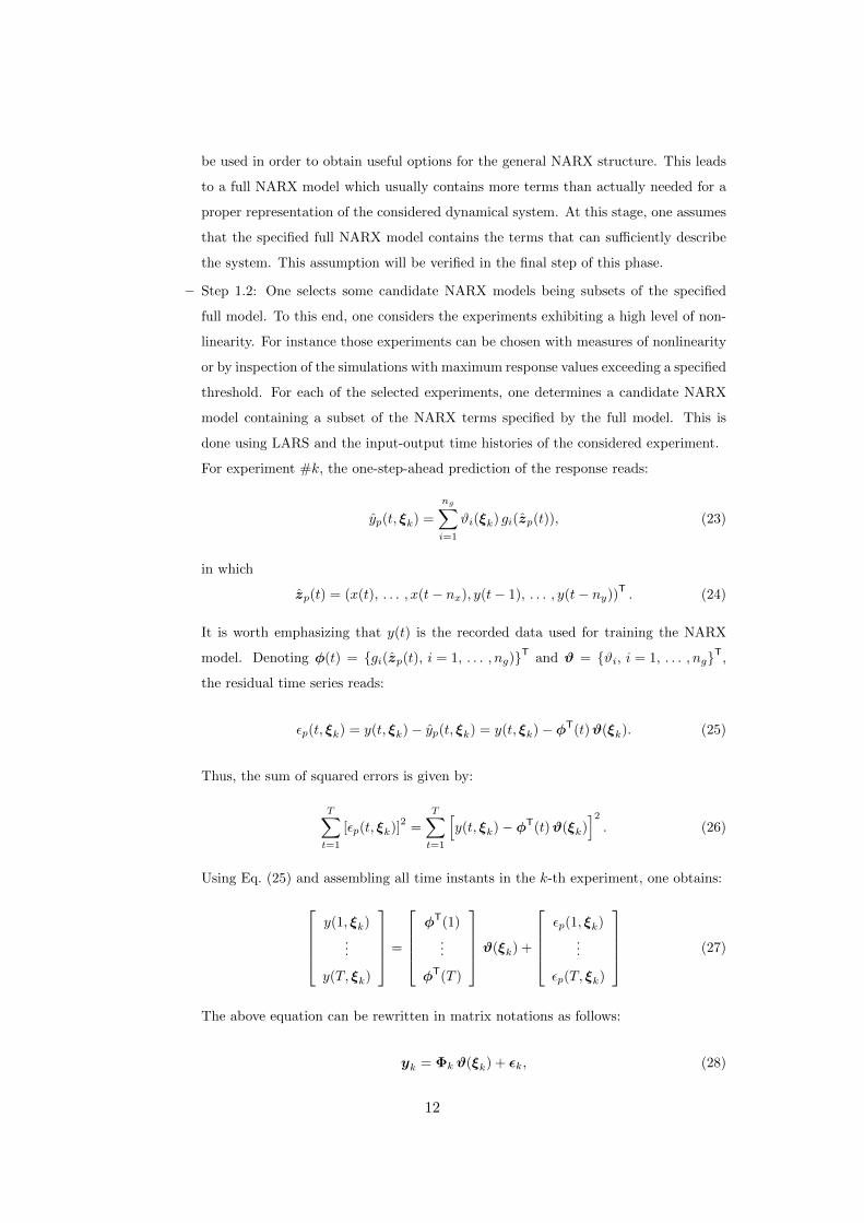
For experiment #k, the one-step-ahead prediction of the response reads:

yp(t, ξk) =

ng∑

i=1

ϑi(ξk) gi(zp(t)), (23)

in which

zp(t) = (x(t), . . . , x(t− nx), y(t− 1), . . . , y(t− ny))T. (24)

It is worth emphasizing that y(t) is the recorded data used for training the NARX

model. Denoting φ(t) = gi(zp(t), i = 1, . . . , ng)T and ϑ = ϑi, i = 1, . . . , ngT,

the residual time series reads:

εp(t, ξk) = y(t, ξk)− yp(t, ξk) = y(t, ξk)− φT(t)ϑ(ξk). (25)

Thus, the sum of squared errors is given by:

T∑

t=1

[εp(t, ξk)]2

=T∑

t=1

[y(t, ξk)− φT(t)ϑ(ξk)

]2. (26)

Using Eq. (25) and assembling all time instants in the k-th experiment, one obtains:

y(1, ξk)...

y(T, ξk)

=

φT(1)...

φT(T )

ϑ(ξk) +

εp(1, ξk)...

εp(T, ξk)

(27)

The above equation can be rewritten in matrix notations as follows:

yk = Φk ϑ(ξk) + εk, (28)

12

where yk is the T ×1 vector of output time-series, Φk is the T ×ng information matrix

with the ith row containing the evaluations of NARX terms φ(t) at instant t = i and

εk is the residual vector. This is typically the equation of a linear regression problem,

for which the relevant NARX regressors among the NARX candidate terms φ(t) can

be selected by LARS.

Note that the same candidate model might be obtained from different selected exper-

iments. In theory all the available experiments can be considered, i.e. the number of

candidate models is at most the size of the ED. Herein, we search for the appropriate

NARX model among a limited number of experiments which are exhibiting strong

non-linearity.

– Step 1.3: For each candidate NARX model, the corresponding NARX coefficients

are computed for each of the experiments by ordinary least-squares. The parameters

ϑ(ξk) minimizing the total errors in Eq. (26) is the least-squares solution of Eq. (28),

i.e. :

ϑ(ξk) = arg minϑ

(εTk εk) =[ΦTk Φk

]−1ΦTk yk, (29)

with the information matrix Φk containing only the NARX regressors specified in the

NARX candidate. Having at hand the NARX coefficients, the free-run reconstruction

for each experiment output is conducted as follows:

ys(t, ξk) =

ng∑

i=1

ϑi(ξk) gi(zs(t)), (30)

in which

zs(t) = (x(t), . . . , x(t− nx), ys(t− 1), . . . , ys(t− ny))T. (31)

It is worth underlining that the free-run reconstruction of the response is obtained

using only the excitation time series x(t) and the response initial condition y0. The

response is reconstructed recursively, i.e. its estimate at one instant is used to predict

the response at later instants. This differs from Eq. (23) where the recorded response

was used in the recursive formulation. The relative error for simulation #k reads:

εk =

T∑t=1

(y(t, ξk)− ys(t, ξk))2

T∑t=1

(y(t, ξk)− y(t, ξk))2, (32)

in which ys(t, ξk) is the output trajectory reconstructed by the NARX model and

y(t, ξk) is the mean value of the response time series y(t, ξk).

– Step 1.4: One selects the most appropriate NARX model among the candidates.

13

Herein, the error criterion of interest is the mean value of the relative errors:

ε =1

K

K∑

k=1

εk. (33)

We propose to choose the model that achieves a sufficiently small overall error on the

conducted experiments, e.g. ε < 1× 10−3, with the smallest number of NARX terms.

In other words, the appropriate model is the simplest one that allows to capture the

system dynamical behaviour, thus following the principle suggested by Billings Billings

(2013).

To refine the estimated coefficients, a nonlinear optimization for minimizing the simu-

lation error (Eq. (32)) may be conducted afterwards Spiridonakos and Chatzi (2015a).

However, this is not used in the current paper due to the fact that LARS allows one

to detect the appropriate NARX terms, therefore the models estimated by ordinary

least-squares appear sufficiently accurate.

If an appropriate NARX model is not obtained, i.e. the initial assumption that the

full NARX model includes an appropriate candidate is not satisfied, the process is

re-started from Step 1.1 (choice of model class), when different options for the full

NARX model should be considered. For instance, one may use more complex models

with larger time lags, different basis functions, etc.

• Phase 2: Representation of the NARX coefficients by means of PCEs using the sparse

adaptive PCE scheme which is based on LARS (see section 2.4). The NARX coefficients

obtained from Phase 1 are used for training the PC expansion.

For the sake of clarity, the above procedure for computing a PC-NARX model is summarized

by the flowchart in Figure 1.

4.2 Use of the surrogate model for prediction

The PC-NARX surrogate model can be used for the prediction1 of the response to a set of

input parameters ξ′. Given the excitation x(t, ξ′x) and the initial conditions of the response

y(t = 1, ξ′) = y0, the output time history of the system can be recursively obtained as follows:

y(t, ξ′) =

ng∑

i=1

nψ∑

j=1

ϑi,jψj(ξ′) gi(z(t, ξ′)), t = 2, . . . , T, (34)

1In what follows, the term “prediction” is employed to refer to the NARX model’s so-called “simulation mode”as addressed in signal processing literature, which stands for the estimation of the response relying only on its initialcondition and feedback of the excitation. The term “prediction” is used however because it is the standard wordingin the surrogate modelling community.

14

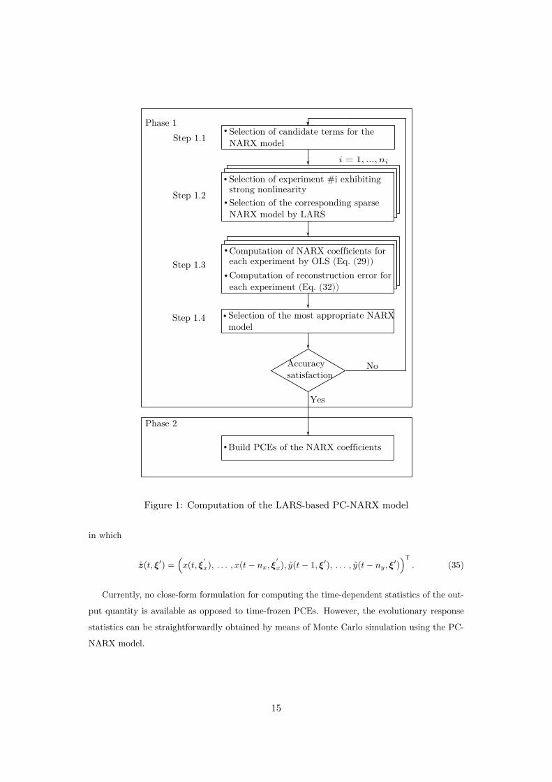
Phase 1 Selection of candidate terms for the NARX modelSelection of experiment #i exhibiting strong nonlinearitySelection of the corresponding sparse NARX model by LARSComputation of NARX coefficients for each experiment by OLS (Eq. (29))Computation of reconstruction error for each experiment (Eq. (32))Selection of the most appropriate NARX model

Accuracy satisfactionBuild PCEs of the NARX coefficientsPhase 2

Step 1.1Step 1.2Step 1.3Step 1.4

NoYes

Figure 1: Computation of the LARS-based PC-NARX model

in which

z(t, ξ′) =(x(t, ξ

′

x), . . . , x(t− nx, ξ′

x), y(t− 1, ξ′), . . . , y(t− ny, ξ′))T

. (35)

Currently, no close-form formulation for computing the time-dependent statistics of the out-

put quantity is available as opposed to time-frozen PCEs. However, the evolutionary response

statistics can be straightforwardly obtained by means of Monte Carlo simulation using the PC-

NARX model.

15

4.3 Validation of the surrogate model

The PC-NARX model is computed using an ED of limited size. The validation process is

conducted with a validation set of large size which is independent of the ED. A large number,

e.g. nval = 104, of input parameters and excitations is generated. One uses the numerical solver

to obtain the response time histories sampled at the discrete time instants t = 1, . . . , T . Then

PC-NARX model (Eq. (34)) is used to predict the time dependent responses to the excitations

and uncertain parameters of the validation set. The accuracy of the computed PC-NARX model

is validated by means of comparing its predictions with the actual responses in terms of the

relative errors and the evolutionary statistics of the response. For prediction #i, the relative

error reads:

εval,i =

T∑t=1

(y(t, ξi)− y(t, ξi))2

T∑t=1

(y(t, ξi)− y(t, ξi))2

, (36)

where y(t, ξi) is the output trajectory predicted by PC-NARX and y(t, ξi) is the mean value of

the actual response time series y(t, ξi). The above formula is also used to calculate the accuracy

of the time dependent statistics (i.e. mean, standard deviation) predicted by PC-NARX. The

mean value of the relative errors over nval predictions reads:

εval =1

nval

nval∑

i=1

εval,i. (37)

The relative error for a quantity y, e.g. the maximal value of the response (resp. the response

at a specified instant) is given by:

εval,y =

nval∑i=1

(yi − yi)2

nval∑i=1

(yi − y)2, (38)

where yi is the actual response, yi is the prediction by PC-NARX and y is the mean value defined

by y =1

nval

nval∑i=1

yi.

5 Numerical applications

The use of LARS-based PC-NARX model is now illustrated with three nonlinear dynamical

systems with increasing complexity, namely a quarter car model subject to a stochastic sinusoidal

road profile, a single degree-of-freedom (SDOF) Duffing and a SDOF Bouc-Wen oscillator subject

to stochastic non-stationary excitation. In all considered numerical examples, uncertainties

arising from the system properties and from the excitation are taken into account. PC-NARX

16

models are computed using a small number of numerical simulations as experimental design.

The validation is conducted by comparing their response predictions with the reference values

obtained by using Monte Carlo simulation (MCS) on the numerical solvers.

5.1 Quarter car model

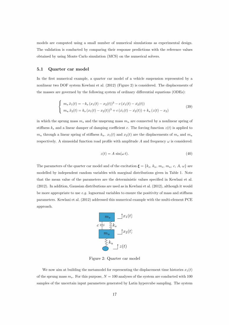
In the first numerical example, a quarter car model of a vehicle suspension represented by a

nonlinear two DOF system Kewlani et al. (2012) (Figure 2) is considered. The displacements of

the masses are governed by the following system of ordinary differential equations (ODEs):

ms x1(t) = −ks (x1(t)− x2(t))3 − c (x1(t)− x2(t))

mu x2(t) = ks (x1(t)− x2(t))3 + c (x1(t)− x2(t)) + ku (z(t)− x2)(39)

in which the sprung mass ms and the unsprung mass mu are connected by a nonlinear spring of

stiffness ks and a linear damper of damping coefficient c. The forcing function z(t) is applied to

mu through a linear spring of stiffness ku. x1(t) and x2(t) are the displacements of ms and mu

respectively. A sinusoidal function road profile with amplitude A and frequency ω is considered:

z(t) = A sin(ω t). (40)

The parameters of the quarter car model and of the excitation ξ = ks, ku, ms, mu, c, A, ω are

modelled by independent random variables with marginal distributions given in Table 1. Note

that the mean value of the parameters are the deterministic values specified in Kewlani et al.

(2012). In addition, Gaussian distributions are used as in Kewlani et al. (2012), although it would

be more appropriate to use e.g. lognormal variables to ensure the positivity of mass and stiffness

parameters. Kewlani et al. (2012) addressed this numerical example with the multi-element PCE

approach.

Figure 2: Quarter car model

We now aim at building the metamodel for representing the displacement time histories x1(t)

of the sprung mass ms. For this purpose, N = 100 analyses of the system are conducted with 100

samples of the uncertain input parameters generated by Latin hypercube sampling. The system

17

Table 1: Parameters of the quarter car model and of the road excitationParameter Distribution Mean & Standard deviation

ks (N/m3) Gaussian (2000, 200)ku (N/m) Gaussian (2000, 200)ms (kg) Gaussian (20, 2)mu (kg) Gaussian (40, 4)c (N s /m) Gaussian (600, 60)

Parameter Distribution Support

A (m) Uniform [0.09, 0.11]ω (rad/s) Uniform [1.8π, 2.2π]

of ODEs are solved by means of the Matlab solver ode45 (explicit Runge-Kutta method with

relative error tolerance 1 × 10−3) for the total duration T = 30 s and the time step dt = 0.01 s.

In the first place, a NARX model structure is chosen, in which the model terms are polynomial

functions of past values of the output and excitation gi(t) = xl1(t− j) zm(t− k) with l+m ≤ 3,

0 ≤ l ≤ 3, 0 ≤ m ≤ 1, j = 1, . . . , 4, k = 0, . . . , 4. The specified full NARX model contains

86 terms. It is worth noticing that the initial choice of the NARX structure was facilitated by

the knowledge of the dynamical nonlinear behaviour of the system of interest. For instance,

polynomial functions of order up to 3 are used because of the cubic nonlinear behaviour as in

Eq. (39). As a rule of thumb, the maximum time lags nx = ny = 4 are chosen equal to twice

the number of degrees of freedom of the considered system.

Next, the candidate NARX models were computed. To this end, we selected the simulations

with maximum displacement exceeding a large threshold, i.e. max(|x1(t)|) > 1.2 m and retained

15 experiments. For each selected simulation, LARS was applied to the initial full NARX model

to detect the most relevant NARX terms constituting a candidate NARX model. This procedure

resulted in 10 different candidate NARX models in total.

For each candidate NARX model, we computed the NARX coefficients for all simulations by

ordinary least-squares to minimize the sum of squared errors (Eq. (29)). We then reconstructed

all the output time histories with the computed coefficients and calculated the relative errors εk

of the reconstruction (Eq. (32)).

Among the 10 candidates, we selected the most appropriate NARX model which achieves a

sufficiently small overall error with the smallest number of terms. The selected model results

in a mean relative error ε = 3.56 × 10−4 for 100 simulations in the ED and contains 6 terms,

namely the constant term, z(t−4), x1(t−4), x1(t−1), x31(t−1), x21(t−4) z(t−4). LARS proves

effective in selecting the appropriate NARX model by retaining only 6 among the 86 candidate

terms available to describe the system.

In the next step, we expanded the 6 NARX coefficients by adaptive sparse PCEs of order

p ≤ 20 with maximum interaction rank r = 2 and truncation parameter q = 1. The NARX

18

coefficients computed in the previous step were used for training the metamodel. PCE models

that minimize the LOO errors were selected. This led to LOO errors smaller than 10−7. The

optimal PCE order selected by the adaptive scheme is up to 6.

For the sake of comparison, we represent the response x1(t) by means of time-frozen PCEs.

For this purpose, adaptive sparse PCEs are used with an ED of size N = 500. The best PCE

with maximum degree 1 6 p 6 20, maximum interaction rank r = 2 and truncation parameter

q = 1 is selected. The PC-NARX and time-frozen PCEs are used to predict the output time

histories for an independent validation set of size nval = 104 which is pre-computed by the

numerical solver. The accuracy of the two PCE approaches are compared in the following.

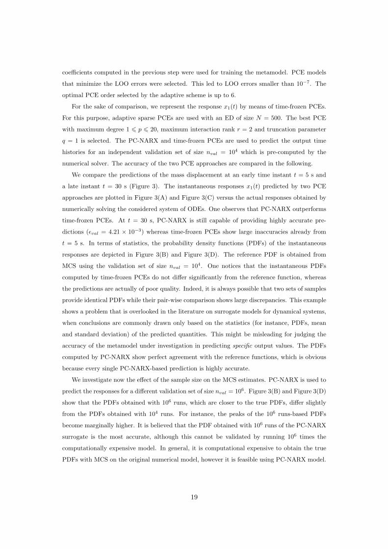
We compare the predictions of the mass displacement at an early time instant t = 5 s and

a late instant t = 30 s (Figure 3). The instantaneous responses x1(t) predicted by two PCE

approaches are plotted in Figure 3(A) and Figure 3(C) versus the actual responses obtained by

numerically solving the considered system of ODEs. One observes that PC-NARX outperforms

time-frozen PCEs. At t = 30 s, PC-NARX is still capable of providing highly accurate pre-

dictions (εval = 4.21 × 10−3) whereas time-frozen PCEs show large inaccuracies already from

t = 5 s. In terms of statistics, the probability density functions (PDFs) of the instantaneous

responses are depicted in Figure 3(B) and Figure 3(D). The reference PDF is obtained from

MCS using the validation set of size nval = 104. One notices that the instantaneous PDFs

computed by time-frozen PCEs do not differ significantly from the reference function, whereas

the predictions are actually of poor quality. Indeed, it is always possible that two sets of samples

provide identical PDFs while their pair-wise comparison shows large discrepancies. This example

shows a problem that is overlooked in the literature on surrogate models for dynamical systems,

when conclusions are commonly drawn only based on the statistics (for instance, PDFs, mean

and standard deviation) of the predicted quantities. This might be misleading for judging the

accuracy of the metamodel under investigation in predicting specific output values. The PDFs

computed by PC-NARX show perfect agreement with the reference functions, which is obvious

because every single PC-NARX-based prediction is highly accurate.

We investigate now the effect of the sample size on the MCS estimates. PC-NARX is used to

predict the responses for a different validation set of size nval = 106. Figure 3(B) and Figure 3(D)

show that the PDFs obtained with 106 runs, which are closer to the true PDFs, differ slightly

from the PDFs obtained with 104 runs. For instance, the peaks of the 106 runs-based PDFs

become marginally higher. It is believed that the PDF obtained with 106 runs of the PC-NARX

surrogate is the most accurate, although this cannot be validated by running 106 times the

computationally expensive model. In general, it is computational expensive to obtain the true

PDFs with MCS on the original numerical model, however it is feasible using PC-NARX model.

19

−3 −2 −1 0 1 2 3−3

−2

−1

0

1

2

3

Actual values

PC

E

Time−frozen PCE, εval

= 9.69e−02

PC−NARX, εval

= 9.86e−04

(A) t = 5 s

−3 −2 −1 0 1 2 30

0.2

0.4

0.6

0.8

1

1.2

1.4

x1(t)

Pro

babili

ty d

ensity function

Reference

Time−frozen PCE

PC−NARX 104 runs

PC−NARX 106 runs

(B) t = 5 s

−3 −2 −1 0 1 2 3−3

−2

−1

0

1

2

3

Actual values

PC

E

Time−frozen PCE, εval

= 6.38e−01

PC−NARX, εval

= 4.21e−03

(C) t = 30 s

−3 −2 −1 0 1 2 30

0.2

0.4

0.6

0.8

1

1.2

x1(t)

Pro

babili

ty d

ensity function

Reference

Time−frozen PCE

PC−NARX 104 runs

PC−NARX 106 runs

(D) t = 30 s

Figure 3: Quarter car model – Instantaneous displacements: comparison of the two approaches.

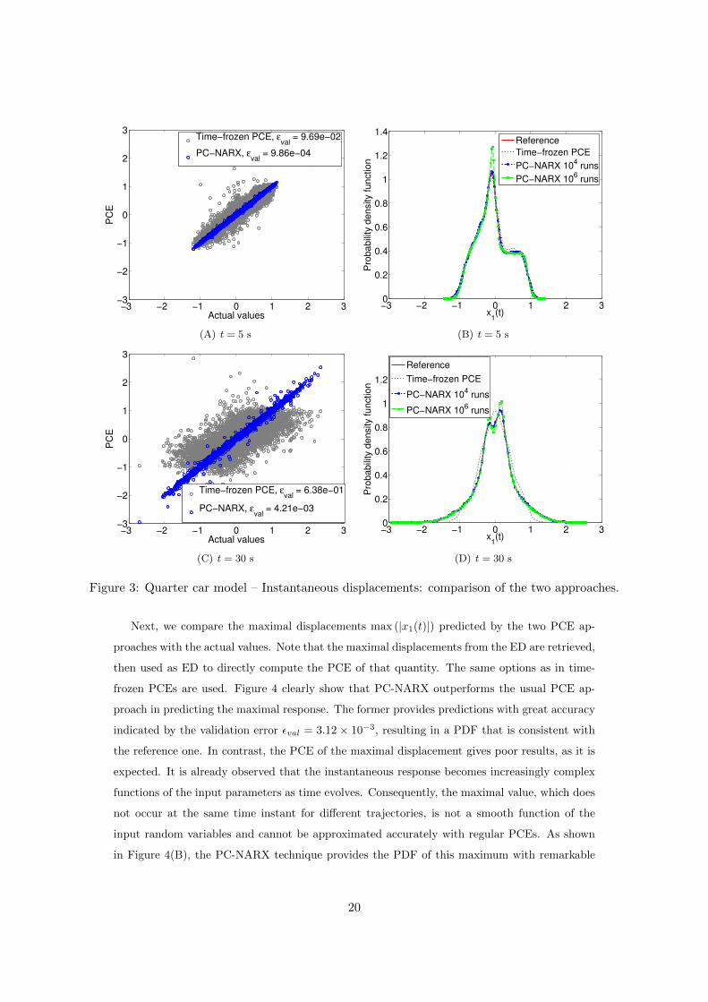
Next, we compare the maximal displacements max (|x1(t)|) predicted by the two PCE ap-

proaches with the actual values. Note that the maximal displacements from the ED are retrieved,

then used as ED to directly compute the PCE of that quantity. The same options as in time-

frozen PCEs are used. Figure 4 clearly show that PC-NARX outperforms the usual PCE ap-

proach in predicting the maximal response. The former provides predictions with great accuracy

indicated by the validation error εval = 3.12× 10−3, resulting in a PDF that is consistent with

the reference one. In contrast, the PCE of the maximal displacement gives poor results, as it is

expected. It is already observed that the instantaneous response becomes increasingly complex

functions of the input parameters as time evolves. Consequently, the maximal value, which does

not occur at the same time instant for different trajectories, is not a smooth function of the

input random variables and cannot be approximated accurately with regular PCEs. As shown

in Figure 4(B), the PC-NARX technique provides the PDF of this maximum with remarkable

20

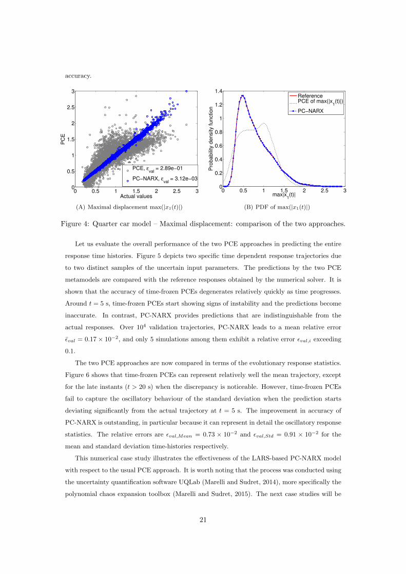
accuracy.

0 0.5 1 1.5 2 2.5 30

0.5

1

1.5

2

2.5

3

Actual values

PC

E

PCE, εval

= 2.89e−01

PC−NARX, εval

= 3.12e−03

(A) Maximal displacement max(|x1(t)|)

0 0.5 1 1.5 2 2.5 30

0.2

0.4

0.6

0.8

1

1.2

1.4

max|x1(t)|

Pro

babili

ty d

ensity function

ReferencePCE of max(|x

1(t)|)

PC−NARX

(B) PDF of max(|x1(t)|)

Figure 4: Quarter car model – Maximal displacement: comparison of the two approaches.

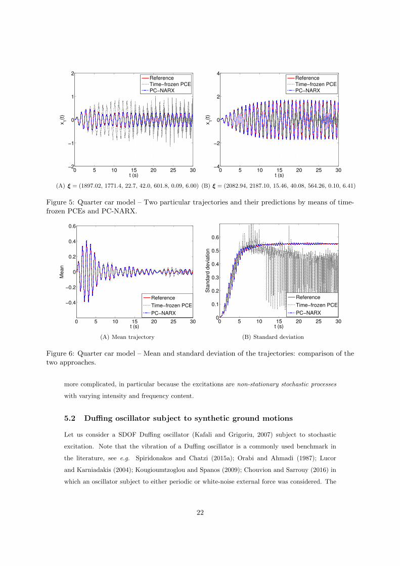
Let us evaluate the overall performance of the two PCE approaches in predicting the entire

response time histories. Figure 5 depicts two specific time dependent response trajectories due

to two distinct samples of the uncertain input parameters. The predictions by the two PCE

metamodels are compared with the reference responses obtained by the numerical solver. It is

shown that the accuracy of time-frozen PCEs degenerates relatively quickly as time progresses.

Around t = 5 s, time-frozen PCEs start showing signs of instability and the predictions become

inaccurate. In contrast, PC-NARX provides predictions that are indistinguishable from the

actual responses. Over 104 validation trajectories, PC-NARX leads to a mean relative error

εval = 0.17 × 10−2, and only 5 simulations among them exhibit a relative error εval,i exceeding

0.1.

The two PCE approaches are now compared in terms of the evolutionary response statistics.

Figure 6 shows that time-frozen PCEs can represent relatively well the mean trajectory, except

for the late instants (t > 20 s) when the discrepancy is noticeable. However, time-frozen PCEs

fail to capture the oscillatory behaviour of the standard deviation when the prediction starts

deviating significantly from the actual trajectory at t = 5 s. The improvement in accuracy of

PC-NARX is outstanding, in particular because it can represent in detail the oscillatory response

statistics. The relative errors are εval,Mean = 0.73 × 10−2 and εval,Std = 0.91 × 10−2 for the

mean and standard deviation time-histories respectively.

This numerical case study illustrates the effectiveness of the LARS-based PC-NARX model

with respect to the usual PCE approach. It is worth noting that the process was conducted using

the uncertainty quantification software UQLab (Marelli and Sudret, 2014), more specifically the

polynomial chaos expansion toolbox (Marelli and Sudret, 2015). The next case studies will be

21

0 5 10 15 20 25 30−2

−1

0

1

2

t (s)

x1(t

)

Reference

Time−frozen PCE

PC−NARX

(A) ξ = (1897.02, 1771.4, 22.7, 42.0, 601.8, 0.09, 6.00)

0 5 10 15 20 25 30−4

−2

0

2

4

t (s)

x1(t

)

Reference

Time−frozen PCE

PC−NARX

(B) ξ = (2082.94, 2187.10, 15.46, 40.08, 564.26, 0.10, 6.41)

Figure 5: Quarter car model – Two particular trajectories and their predictions by means of time-frozen PCEs and PC-NARX.

0 5 10 15 20 25 30

−0.4

−0.2

0

0.2

0.4

0.6

t (s)

Me

an

Reference

Time−frozen PCE

PC−NARX

(A) Mean trajectory

0 5 10 15 20 25 300

0.1

0.2

0.3

0.4

0.5

0.6

t (s)

Sta

nd

ard

de

via

tio

n

Reference

Time−frozen PCE

PC−NARX

(B) Standard deviation

Figure 6: Quarter car model – Mean and standard deviation of the trajectories: comparison of thetwo approaches.

more complicated, in particular because the excitations are non-stationary stochastic processes

with varying intensity and frequency content.

5.2 Duffing oscillator subject to synthetic ground motions

Let us consider a SDOF Duffing oscillator (Kafali and Grigoriu, 2007) subject to stochastic

excitation. Note that the vibration of a Duffing oscillator is a commonly used benchmark in

the literature, see e.g. Spiridonakos and Chatzi (2015a); Orabi and Ahmadi (1987); Lucor

and Karniadakis (2004); Kougioumtzoglou and Spanos (2009); Chouvion and Sarrouy (2016) in

which an oscillator subject to either periodic or white-noise external force was considered. The

22

dynamics of the oscillator can be described by the following equation of motion:

y(t) + 2 ζ ω y(t) + ω2 (y(t) + ε y(t)3) = −x(t), (41)

in which y(t) is the oscillator displacement, ζ is the damping ratio, ω is the fundamental fre-

quency, ε is the parameter governing the nonlinear behaviour and x(t) is the excitation.

Herein, the excitation is generated by the probabilistic ground motion model proposed by

Rezaeian and Der Kiureghian (2010). The ground motion acceleration is represented as a non-

stationary process by means of a modulated filtered white noise process as follows:

x(t) = q(t,α)

1

σh(t)

t∫

−∞

h[t− τ,λ(τ)]ω(τ) dτ

. (42)

The white-noise process denoted by ω(τ) passes a filter h[t − τ,λ(τ)] which is selected as an

impulse-response function:

h[t− τ,λ(τ)] =ωf (τ)√1− ζ2f (t)

exp[−ζf (τ)ωf (τ)(t− τ)]

× sin[ωf (τ)√

1− ζ2f (τ)(t− τ)] for τ ≤ t,

h[t− τ,λ(τ)] = 0 for τ > t,

(43)

where λ(τ) = (ωf (τ), ζf (τ)) is the vector of time-varying parameters of the filter h. ωf (τ) and

ζf (τ) are respectively the filter’s frequency and bandwidth at time instant τ . They represent

the evolving predominant frequency and bandwidth of the ground motion. A linear model is

assumed for ωf (τ) and ζf (τ) is constant during the entire signal duration:

ωf (τ) = ωmid + ω′(τ − tmid) and ζf (τ) = ζf , (44)

in which tmid is the instant at which 45% of the expected Arias intensity Ia is reached, ωmid is

the filter frequency at instant tmid and ω′ is the slope of linear evolution of ωf (τ). After being

normalized by the standard deviation σh(t), the integral in Eq. (42) becomes a unit variance

process with time-varying frequency and constant bandwidth, which represents the spectral non-

stationarity of the ground motion.

The non-stationarity in intensity is then captured by the modulation function q(t,α). This

time-modulating function determines the shape, intensity and duration of the motion as follows:

q(t,α) = α1tα2−1exp(−α3 t). (45)

23

The vector of parameters α = (α1, α2, α3) is directly related to the physical characteristics of

the ground motion, namely the expected Arias intensity Ia, the time interval D5−95 between the

instants at which the 5% and 95% of Ia are reached and the instant tmid.

In the discrete time domain, the synthetic ground motion in Eq. (42) becomes:

x(t) = q(t,α)n∑

i=1

si(t, λ(ti))Ui, (46)

where the standard normal random variable Ui represents an impulse at instant ti and si(t, λ(ti))

is given by:

si(t, λ(ti)) =h[t− ti, λ(ti)]√∑kj=1 h

2[t− tj , λ(tj)]for ti < tk, tk ≤ t < tk+1, (47)

= 0 for t ≤ ti.

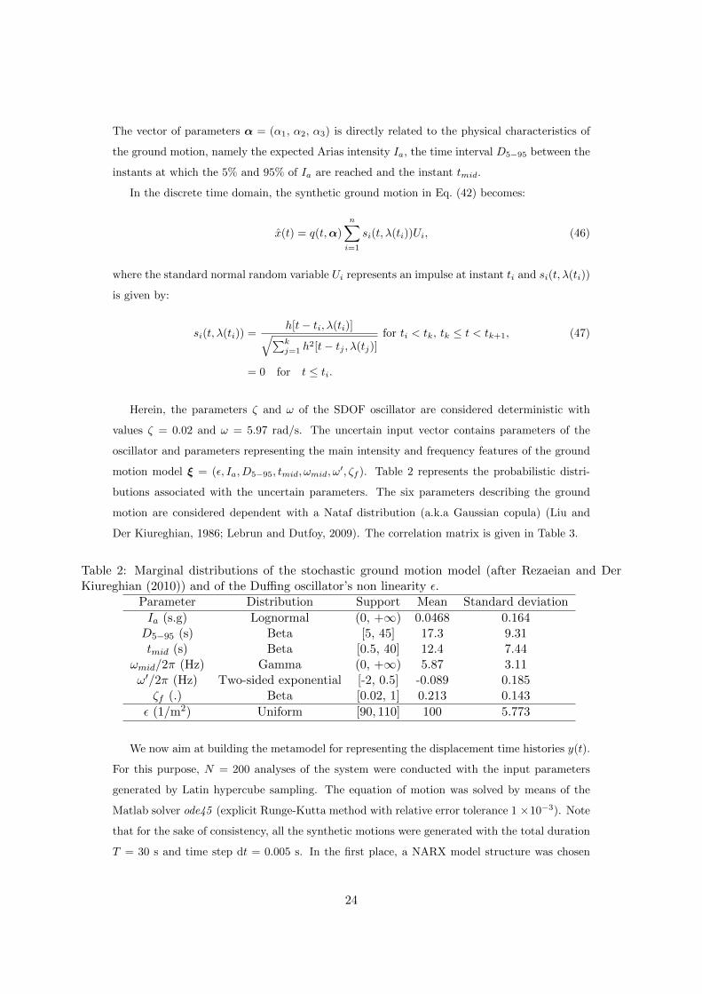
Herein, the parameters ζ and ω of the SDOF oscillator are considered deterministic with

values ζ = 0.02 and ω = 5.97 rad/s. The uncertain input vector contains parameters of the

oscillator and parameters representing the main intensity and frequency features of the ground

motion model ξ = (ε, Ia, D5−95, tmid, ωmid, ω′, ζf ). Table 2 represents the probabilistic distri-

butions associated with the uncertain parameters. The six parameters describing the ground

motion are considered dependent with a Nataf distribution (a.k.a Gaussian copula) (Liu and

Der Kiureghian, 1986; Lebrun and Dutfoy, 2009). The correlation matrix is given in Table 3.

Table 2: Marginal distributions of the stochastic ground motion model (after Rezaeian and DerKiureghian (2010)) and of the Duffing oscillator’s non linearity ε.

Parameter Distribution Support Mean Standard deviation

Ia (s.g) Lognormal (0, +∞) 0.0468 0.164D5−95 (s) Beta [5, 45] 17.3 9.31tmid (s) Beta [0.5, 40] 12.4 7.44

ωmid/2π (Hz) Gamma (0, +∞) 5.87 3.11ω′/2π (Hz) Two-sided exponential [-2, 0.5] -0.089 0.185ζf (.) Beta [0.02, 1] 0.213 0.143

ε (1/m2) Uniform [90, 110] 100 5.773

We now aim at building the metamodel for representing the displacement time histories y(t).

For this purpose, N = 200 analyses of the system were conducted with the input parameters

generated by Latin hypercube sampling. The equation of motion was solved by means of the

Matlab solver ode45 (explicit Runge-Kutta method with relative error tolerance 1 ×10−3). Note

that for the sake of consistency, all the synthetic motions were generated with the total duration

T = 30 s and time step dt = 0.005 s. In the first place, a NARX model structure was chosen

24

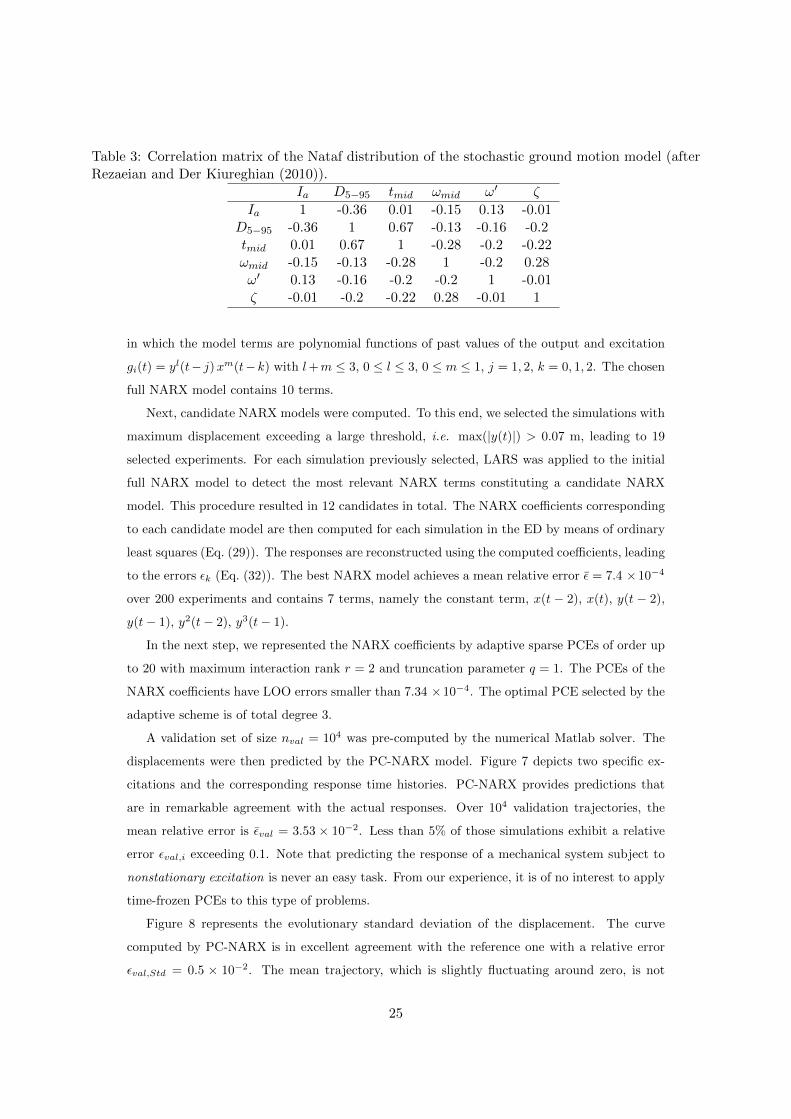
Table 3: Correlation matrix of the Nataf distribution of the stochastic ground motion model (afterRezaeian and Der Kiureghian (2010)).

Ia D5−95 tmid ωmid ω′ ζ

Ia 1 -0.36 0.01 -0.15 0.13 -0.01D5−95 -0.36 1 0.67 -0.13 -0.16 -0.2tmid 0.01 0.67 1 -0.28 -0.2 -0.22ωmid -0.15 -0.13 -0.28 1 -0.2 0.28ω′ 0.13 -0.16 -0.2 -0.2 1 -0.01ζ -0.01 -0.2 -0.22 0.28 -0.01 1

in which the model terms are polynomial functions of past values of the output and excitation

gi(t) = yl(t− j)xm(t−k) with l+m ≤ 3, 0 ≤ l ≤ 3, 0 ≤ m ≤ 1, j = 1, 2, k = 0, 1, 2. The chosen

full NARX model contains 10 terms.

Next, candidate NARX models were computed. To this end, we selected the simulations with

maximum displacement exceeding a large threshold, i.e. max(|y(t)|) > 0.07 m, leading to 19

selected experiments. For each simulation previously selected, LARS was applied to the initial

full NARX model to detect the most relevant NARX terms constituting a candidate NARX

model. This procedure resulted in 12 candidates in total. The NARX coefficients corresponding

to each candidate model are then computed for each simulation in the ED by means of ordinary

least squares (Eq. (29)). The responses are reconstructed using the computed coefficients, leading

to the errors εk (Eq. (32)). The best NARX model achieves a mean relative error ε = 7.4 ×10−4

over 200 experiments and contains 7 terms, namely the constant term, x(t − 2), x(t), y(t − 2),

y(t− 1), y2(t− 2), y3(t− 1).

In the next step, we represented the NARX coefficients by adaptive sparse PCEs of order up

to 20 with maximum interaction rank r = 2 and truncation parameter q = 1. The PCEs of the

NARX coefficients have LOO errors smaller than 7.34 ×10−4. The optimal PCE selected by the

adaptive scheme is of total degree 3.

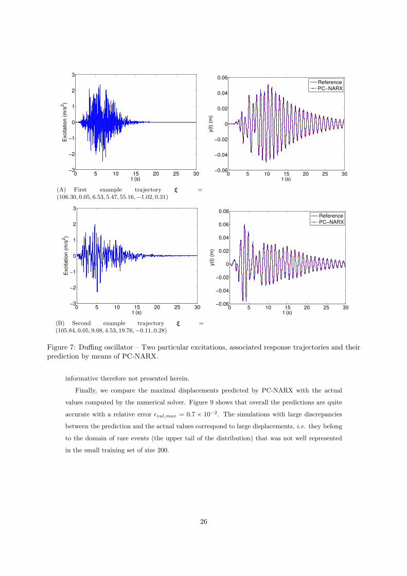
A validation set of size nval = 104 was pre-computed by the numerical Matlab solver. The

displacements were then predicted by the PC-NARX model. Figure 7 depicts two specific ex-

citations and the corresponding response time histories. PC-NARX provides predictions that

are in remarkable agreement with the actual responses. Over 104 validation trajectories, the

mean relative error is εval = 3.53 × 10−2. Less than 5% of those simulations exhibit a relative

error εval,i exceeding 0.1. Note that predicting the response of a mechanical system subject to

nonstationary excitation is never an easy task. From our experience, it is of no interest to apply

time-frozen PCEs to this type of problems.

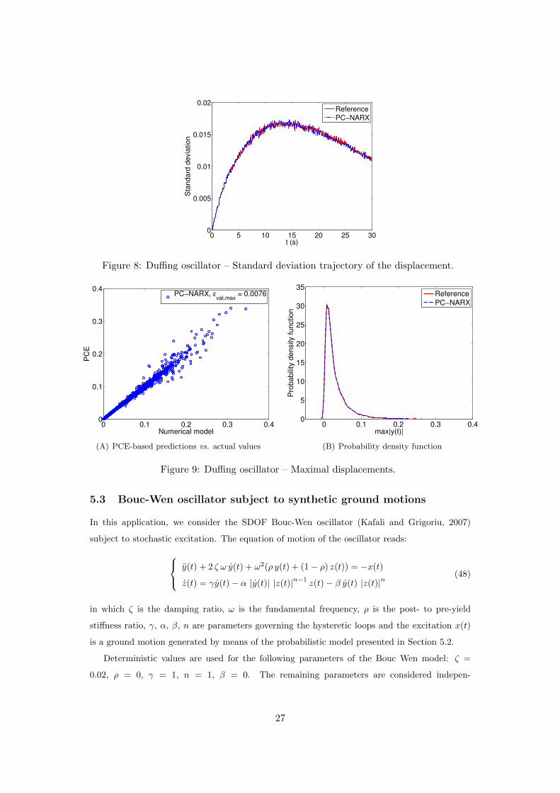
Figure 8 represents the evolutionary standard deviation of the displacement. The curve

computed by PC-NARX is in excellent agreement with the reference one with a relative error

εval,Std = 0.5 × 10−2. The mean trajectory, which is slightly fluctuating around zero, is not

25

0 5 10 15 20 25 30−3

−2

−1

0

1

2

3

t (s)

Excitation (

m/s

2)

(A) First example trajectory ξ =(106.30, 0.05, 6.53, 5.47, 55.16,−1.02, 0.31)

0 5 10 15 20 25 30−0.06

−0.04

−0.02

0

0.02

0.04

0.06

t (s)

y(t

) (m

)

Reference

PC−NARX

0 5 10 15 20 25 30−3

−2

−1

0

1

2

3

t (s)

Excitation (

m/s

2)

(B) Second example trajectory ξ =(105.84, 0.05, 9.08, 4.53, 19.76,−0.11, 0.28)

0 5 10 15 20 25 30−0.06

−0.04

−0.02

0

0.02

0.04

0.06

0.08

t (s)

y(t

) (m

)

Reference

PC−NARX

Figure 7: Duffing oscillator – Two particular excitations, associated response trajectories and theirprediction by means of PC-NARX.

informative therefore not presented herein.

Finally, we compare the maximal displacements predicted by PC-NARX with the actual

values computed by the numerical solver. Figure 9 shows that overall the predictions are quite

accurate with a relative error εval,max = 0.7 × 10−2. The simulations with large discrepancies

between the prediction and the actual values correspond to large displacements, i.e. they belong

to the domain of rare events (the upper tail of the distribution) that was not well represented

in the small training set of size 200.

26

0 5 10 15 20 25 300

0.005

0.01

0.015

0.02

t (s)

Sta

ndard

devia

tion

Reference

PC−NARX

Figure 8: Duffing oscillator – Standard deviation trajectory of the displacement.

0 0.1 0.2 0.3 0.40

0.1

0.2

0.3

0.4

Numerical model

PC

E

PC−NARX, εval,max

= 0.0076

(A) PCE-based predictions vs. actual values

0 0.1 0.2 0.3 0.40

5

10

15

20

25

30

35

max|y(t)|

Pro

babili

ty d

ensity function

Reference

PC−NARX

(B) Probability density function

Figure 9: Duffing oscillator – Maximal displacements.

5.3 Bouc-Wen oscillator subject to synthetic ground motions

In this application, we consider the SDOF Bouc-Wen oscillator (Kafali and Grigoriu, 2007)

subject to stochastic excitation. The equation of motion of the oscillator reads:

y(t) + 2 ζ ω y(t) + ω2(ρ y(t) + (1− ρ) z(t)) = −x(t)

z(t) = γy(t)− α |y(t)| |z(t)|n−1 z(t)− β y(t) |z(t)|n(48)

in which ζ is the damping ratio, ω is the fundamental frequency, ρ is the post- to pre-yield

stiffness ratio, γ, α, β, n are parameters governing the hysteretic loops and the excitation x(t)

is a ground motion generated by means of the probabilistic model presented in Section 5.2.

Deterministic values are used for the following parameters of the Bouc Wen model: ζ =

0.02, ρ = 0, γ = 1, n = 1, β = 0. The remaining parameters are considered indepen-

27

dent random variables with associated distributions given in Table 4. The uncertainties in

the considered system is therefore characterized by means of vector of uncertain parameters

ξ = (ω, α, Ia, D5−95, tmid, ωmid, ω′, ζ).

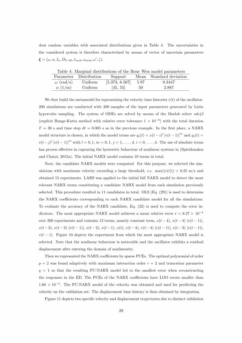
Table 4: Marginal distributions of the Bouc Wen model parametersParameter Distribution Support Mean Standard deviation

ω (rad/s) Uniform [5.373, 6.567] 5.97 0.3447α (1/m) Uniform [45, 55] 50 2.887

We first build the metamodel for representing the velocity time histories v(t) of the oscillator.

200 simulations are conducted with 200 samples of the input parameters generated by Latin

hypercube sampling. The system of ODEs are solved by means of the Matlab solver ode45

(explicit Runge-Kutta method with relative error tolerance 1 × 10−3) with the total duration

T = 30 s and time step dt = 0.005 s as in the previous example. In the first place, a NARX

model structure is chosen, in which the model terms are gi(t) = x(t− i)l |v(t− 1)|m and gi(t) =

v(t− j)l |v(t− 1)|m with l = 0, 1, m = 0, 1, j = 1, . . . , 4, i = 0, . . . , 4. The use of absolute terms

has proven effective in capturing the hysteretic behaviour of nonlinear systems in (Spiridonakos

and Chatzi, 2015a). The initial NARX model contains 19 terms in total.

Next, the candidate NARX models were computed. For this purpose, we selected the sim-

ulations with maximum velocity exceeding a large threshold, i.e. max(|v(t)|) > 0.25 m/s and

obtained 15 experiments. LARS was applied to the initial full NARX model to detect the most

relevant NARX terms constituting a candidate NARX model from each simulation previously

selected. This procedure resulted in 11 candidates in total. OLS (Eq. (29)) is used to determine

the NARX coefficients corresponding to each NARX candidate model for all the simulations.

To evaluate the accuracy of the NARX candidate, Eq. (32) is used to compute the error in-

dicators. The most appropriate NARX model achieves a mean relative error ε = 6.27 × 10−4

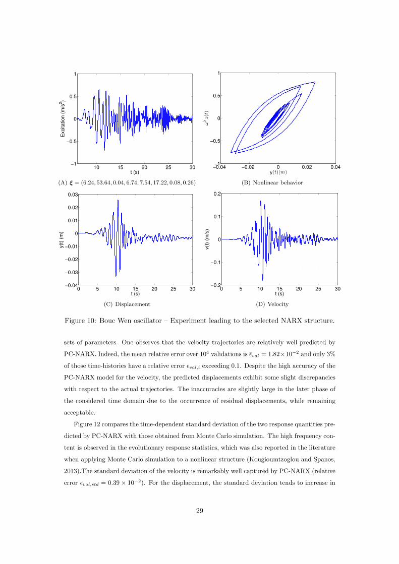
over 200 experiments and contains 12 terms, namely constant term, x(t− 4), x(t− 4) |v(t− 1)|,x(t−3), x(t−3) |v(t− 1)|, x(t−2), x(t−1), x(t), v(t−4), v(t−4) |v(t− 1)|, v(t−3) |v(t− 1)|,v(t − 1). Figure 10 depicts the experiment from which the most appropriate NARX model is

selected. Note that the nonlinear behaviour is noticeable and the oscillator exhibits a residual

displacement after entering the domain of nonlinearity.

Then we represented the NARX coefficients by sparse PCEs. The optimal polynomial of order

p = 2 was found adaptively with maximum interaction order r = 2 and truncation parameter

q = 1 so that the resulting PC-NARX model led to the smallest error when reconstructing

the responses in the ED. The PCEs of the NARX coefficients have LOO errors smaller than

1.68 × 10−4. The PC-NARX model of the velocity was obtained and used for predicting the

velocity on the validation set. The displacement time history is then obtained by integration.

Figure 11 depicts two specific velocity and displacement trajectories due to distinct validation

28

10 15 20 25 30−1

−0.5

0

0.5

1

t (s)

Excita

tio

n (

m/s

2)

(A) ξ = (6.24, 53.64, 0.04, 6.74, 7.54, 17.22, 0.08, 0.26)

−0.04 −0.02 0 0.02 0.04−1

−0.5

0

0.5

1

y(t)(m)

ω2z(t)

(B) Nonlinear behavior

0 5 10 15 20 25 30−0.04

−0.03

−0.02

−0.01

0

0.01

0.02

0.03

t (s)

y(t

) (m

)

(C) Displacement

0 5 10 15 20 25 30−0.2

−0.1

0

0.1

0.2

t (s)

v(t

) (m

/s)

(D) Velocity

Figure 10: Bouc Wen oscillator – Experiment leading to the selected NARX structure.

sets of parameters. One observes that the velocity trajectories are relatively well predicted by

PC-NARX. Indeed, the mean relative error over 104 validations is εval = 1.82×10−2 and only 3%

of those time-histories have a relative error εval,i exceeding 0.1. Despite the high accuracy of the

PC-NARX model for the velocity, the predicted displacements exhibit some slight discrepancies

with respect to the actual trajectories. The inaccuracies are slightly large in the later phase of

the considered time domain due to the occurrence of residual displacements, while remaining

acceptable.

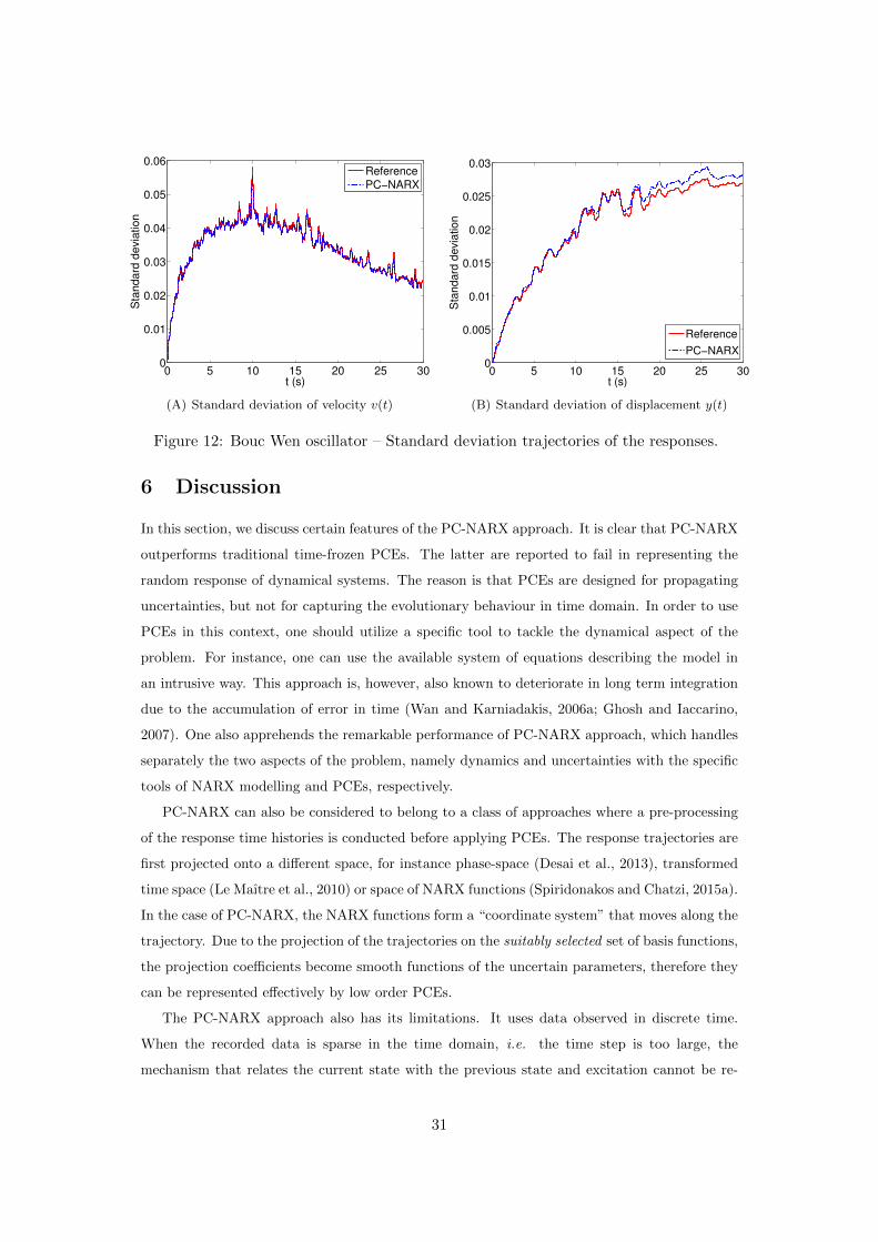
Figure 12 compares the time-dependent standard deviation of the two response quantities pre-

dicted by PC-NARX with those obtained from Monte Carlo simulation. The high frequency con-

tent is observed in the evolutionary response statistics, which was also reported in the literature

when applying Monte Carlo simulation to a nonlinear structure (Kougioumtzoglou and Spanos,

2013).The standard deviation of the velocity is remarkably well captured by PC-NARX (relative

error εval,std = 0.39 × 10−2). For the displacement, the standard deviation tends to increase in

29

time, which is different from the Duffing oscillator that does not exhibit residual displacement.

The discrepancy between the prediction and the actual time histories is also increasing in time.

However, the resulting relative error remains rather small (εval,mean = 1.57× 10−2).

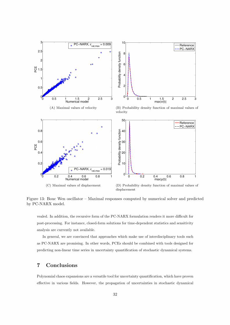
Figure 13 compares the maximum values of velocity and displacement predicted by PC-NARX

with those values computed by the numerical solver. Despite the complexity of the problem,

the predictions are remarkably consistent with the true values, with sufficiently small validation

errors of εval,max(|v(t)|) = 9 × 10−3 and εval,max(|y(t)|) = 1.9 × 10−2. The accurate predictions

allow one to obtain the probability density functions of the maximum responses that are in good

agreement with the reference functions, as shown in Figure 13(B) and Figure 13(D).

0 5 10 15 20 25 30−0.15

−0.1

−0.05

0

0.05

0.1

0.15

0.2

t (s)

v(t

) (m

/s)

Reference

PC−NARX

(A) First example trajectory ξ =(6.35, 46.54, 0.05, 6.53, 5.47, 55.16,−1.02, 0.31)

0 5 10 15 20 25 30−0.02

−0.01

0

0.01

0.02

0.03

0.04

t (s)

y(t

) (m

)

Reference

PC−NARX

0 5 10 15 20 25 30−0.2

−0.1

0

0.1

0.2

0.3

t (s)

v(t

) (m

/s)

Reference

PC−NARX

(B) Second example trajectory ξ =(6.32, 48.24, 0.05, 9.08, 4.53, 19.76,−0.11, 0.28)

0 5 10 15 20 25 30−0.06

−0.04

−0.02

0

0.02

t (s)

y(t

) (m

)

Reference

PC−NARX

Figure 11: Bouc Wen oscillator – Two particular trajectories of velocity v(t) and displacement y(t)and their predictions by means of PC-NARX.

30

0 5 10 15 20 25 300

0.01

0.02

0.03

0.04

0.05

0.06

t (s)

Sta

ndard

devia

tion

Reference

PC−NARX

(A) Standard deviation of velocity v(t)

0 5 10 15 20 25 300

0.005

0.01

0.015

0.02

0.025

0.03

t (s)

Sta

ndard

devia

tion

Reference

PC−NARX

(B) Standard deviation of displacement y(t)

Figure 12: Bouc Wen oscillator – Standard deviation trajectories of the responses.

6 Discussion

In this section, we discuss certain features of the PC-NARX approach. It is clear that PC-NARX

outperforms traditional time-frozen PCEs. The latter are reported to fail in representing the

random response of dynamical systems. The reason is that PCEs are designed for propagating

uncertainties, but not for capturing the evolutionary behaviour in time domain. In order to use

PCEs in this context, one should utilize a specific tool to tackle the dynamical aspect of the

problem. For instance, one can use the available system of equations describing the model in

an intrusive way. This approach is, however, also known to deteriorate in long term integration

due to the accumulation of error in time (Wan and Karniadakis, 2006a; Ghosh and Iaccarino,

2007). One also apprehends the remarkable performance of PC-NARX approach, which handles

separately the two aspects of the problem, namely dynamics and uncertainties with the specific

tools of NARX modelling and PCEs, respectively.

PC-NARX can also be considered to belong to a class of approaches where a pre-processing

of the response time histories is conducted before applying PCEs. The response trajectories are

first projected onto a different space, for instance phase-space (Desai et al., 2013), transformed

time space (Le Maıtre et al., 2010) or space of NARX functions (Spiridonakos and Chatzi, 2015a).

In the case of PC-NARX, the NARX functions form a “coordinate system” that moves along the

trajectory. Due to the projection of the trajectories on the suitably selected set of basis functions,

the projection coefficients become smooth functions of the uncertain parameters, therefore they

can be represented effectively by low order PCEs.

The PC-NARX approach also has its limitations. It uses data observed in discrete time.

When the recorded data is sparse in the time domain, i.e. the time step is too large, the

mechanism that relates the current state with the previous state and excitation cannot be re-

31

0 0.5 1 1.5 2 2.5 30

0.5

1

1.5

2

2.5

3

Numerical model

PC

E

PC−NARX, εval,max

= 0.009

(A) Maximal values of velocity

0 0.5 1 1.5 2 2.5 30

2

4

6

8

10

max|v(t)|

Pro

babili

ty d

ensity function

Reference

PC−NARX

(B) Probability density function of maximal values ofvelocity

0 0.2 0.4 0.6 0.8 10

0.2

0.4

0.6

0.8

1

Numerical model

PC

E

PC−NARX, εval,max

= 0.019

(C) Maximal values of displacement

0 0.2 0.4 0.6 0.8 10

10

20

30

40

50

max|y(t)|

Pro

babili

ty d

ensity function

Reference

PC−NARX

(D) Probability density function of maximal values ofdisplacement

Figure 13: Bouc Wen oscillator – Maximal responses computed by numerical solver and predictedby PC-NARX model.

vealed. In addition, the recursive form of the PC-NARX formulation renders it more difficult for

post-processing. For instance, closed-form solutions for time-dependent statistics and sensitivity

analysis are currently not available.

In general, we are convinced that approaches which make use of interdisciplinary tools such

as PC-NARX are promising. In other words, PCEs should be combined with tools designed for

predicting non-linear time series in uncertainty quantification of stochastic dynamical systems.

7 Conclusions

Polynomial chaos expansions are a versatile tool for uncertainty quantification, which have proven

effective in various fields. However, the propagation of uncertainties in stochastic dynamical

32

systems remains a challenging issue for PCEs as well as all other metamodelling techniques. It

is widely known that PCEs fail to capture the long-term dynamics of the underlying system.

Therefore, a specialized tool must be used to handle this aspect of the problem. Nonlinear

autoregressive with exogenous input (NARX) models are universally used in the field of system

identification for revealing the dynamical behaviour from observed time series. The combination

of NARX and PCEs have been proposed recently and shown great effectiveness in the context

of stochastic dynamics.

In this paper we introduced the least angle regression (LARS) technique for building PC-

NARX models of nonlinear systems with uncertainties subject to stochastic excitations. In

particular, the approach consists in solving two linear regression problems. LARS proves suit-

able for selecting both the appropriate NARX and PCE models, which plays a crucial role in

the approach. The LARS-based PC-NARX approach is applied to predict the response time

histories of three benchmark engineering models subject to non-stationary stochastic excitation

with remarkable accuracy. It is important to observe that, to our knowledge, no generic non-

intrusive tools based on PCEs were available so far to build surrogate models of dynamical

system responses based on a set of computer experiment.

Investigation on the application of the proposed approach to more complex problems is

ongoing, with particular interests being focused on the seismic analysis of structures.

References

Abramowitz, M. and I. Stegun (1970). Handbook of mathematical functions. Dover Publications,

Inc.

Billings, S. A. (2013). Nonlinear system identification: NARMAX methods in the time, frequency,

and spatio-temporal domains. John Wiley & Sons.

Billings, S. A. and H. L. Wei (2008). An adaptive orthogonal search algorithm for model subset

selection and non-linear system identification. Int. J. Control 81 (5), 714–724.

Blatman, G. (2009). Adaptive sparse polynomial chaos expansions for uncertainty propagation

and sensitivity analysis. Ph. D. thesis, Universite Blaise Pascal, Clermont-Ferrand.

Blatman, G. and B. Sudret (2010). An adaptive algorithm to build up sparse polynomial chaos

expansions for stochastic finite element analysis. Prob. Eng. Mech. 25, 183–197.

Blatman, G. and B. Sudret (2011). Adaptive sparse polynomial chaos expansion based on Least

Angle Regression. J. Comput. Phys 230, 2345–2367.

33

Chen, S., S. A. Billings, and W. Luo (1989). Orthogonal least squares methods and their

application to non-linear system identification. Int. J. Control 50 (5), 1873–1896.

Chen, Z. H. and Y. Q. Ni (2011). On-board identification and control performance verification

of an MR damper incorporated with structure. J. Intel. Mat. Syst. Str. 22 (14), 1551–1565.

Chouvion, B. and E. Sarrouy (2016). Development of error criteria for adaptive multi-element

polynomial chaos approaches. Mech. Syst. Signal Pr. 66-67, 201–222.

Desai, A., J. A. S. Witteveen, and S. Sarkar (2013). Uncertainty quantification of a nonlinear

aeroelastic system using polynomial chaos expansion with constant phase interpolation. J.

Vib. Acoust. 135 (5), 51034.

Efron, B., T. Hastie, I. Johnstone, and R. Tibshirani (2004). Least angle regression. Annals of

Statistics 32, 407–499.

Gerritsma, M., J.-B. van der Steen, P. Vos, and G. Karniadakis (2010). Time-dependent gener-

alized polynomial chaos. J. Comput. Phys 229 (22), 8333–8363.

Ghanem, R., S. Masri, M. Pellissetti, and R. Wolfe (2005). Identification and prediction of

stochastic dynamical systems in a polynomial chaos basis. Comput. Methods Appl. Mech.

Engrg. 194, 1641–1654.

Ghanem, R. and P. Spanos (2003). Stochastic Finite Elements: A Spectral Approach (2nd ed.).

Courier Dover Publications, Mineola.

Ghosh, D. and G. Iaccarino (2007). Applicability of the spectral stochastic finite element method

in time-dependent uncertain problems. Annual Research Briefs of Center for Turbulence

Research, 133–141.

Jacquelin, E., S. Adhikari, J.-J. Sinou, and M. I. Friswell (2015). Polynomial chaos expansion

and steady-state response of a class of random dynamical systems. J. Eng. Mech. 141 (4),

04014145.

Jiang, X. Q. and G. Kitagawa (1993). A time varying coefficient vector AR modeling of nonsta-

tionary covariance time series. Signal Processing 33 (3), 315–331.

Kafali, C. and M. Grigoriu (2007). Seismic fragility analysis: Application to simple linear and

nonlinear systems. Earthquake Eng. Struct. Dyn. 36 (13), 1885–1900.

Kewlani, G., J. Crawford, and K. Iagnemma (2012). A polynomial chaos approach to the analysis

of vehicle dynamics under uncertainty. Vehicle Syst. Dyn. 50 (5), 749–774.

34

Kopsaftopoulos, F. and S. Fassois (2013). A functional model based statistical time series method

for vibration based damage detection, localization, and magnitude estimation. Mech. Syst.

Signal Pr. 39 (1-2), 143–161.

Kougioumtzoglou, I. A. and P. D. Spanos (2009). An approximate approach for nonlinear system

response determination under evolutionary stochastic excitation. Current science 97 (8), 1203–

1211.

Kougioumtzoglou, I. A. and P. D. Spanos (2013). Nonlinear MDOF system stochastic response

determination via a dimension reduction approach. Comput. Struct. 126, 135–148.

Kumar, D. and H. Budman (2014). Robust nonlinear MPC based on Volterra series and poly-

nomial chaos expansions. J. Process Contr. 24 (1), 304–317.

Le Maıtre, O., L. Mathelin, O. Knio, and M. Hussaini (2010). Asynchronous time integration

for polynomial chaos expansion of uncertain periodic dynamics. Discret. Contin. Dyn. Sys. -

Series A (DCDS-A) 28 (1), 199–226.

Lebrun, R. and A. Dutfoy (2009). An innovating analysis of the Nataf transformation from the

copula viewpoint. Prob. Eng. Mech. 24 (3), 312–320.

Liu, P.-L. and A. Der Kiureghian (1986). Multivariate distribution models with prescribed

marginals and covariances. Prob. Eng. Mech. 1 (2), 105–112.

Luchtenburg, D. M., S. L. Brunton, and C. W. Rowley (2014). Long-time uncertainty propa-

gation using generalized polynomial chaos and flow map composition. J. Comp. Phys. 274,

783–802.

Lucor, D. and G. Karniadakis (2004). Adaptive generalized polynomial chaos for nonlinear

random oscillators. SIAM J. Sci. Comput. 26 (2), 720–735.

Marelli, S. and B. Sudret (2014). UQLab: A framework for uncertainty quantification in Matlab.

In Vulnerability, Uncertainty, and Risk (Proc. 2nd Int. Conf. on Vulnerability, Risk Analysis

and Management (ICVRAM2014), Liverpool, United Kingdom), pp. 2554–2563.

Marelli, S. and B. Sudret (2015). UQLab user manual – Polynomial chaos expansions. Technical

report, Chair of Risk, Safety & Uncertainty Quantification, ETH Zurich. Report # UQLab-

V0.9-104.

Orabi, I. I. and G. Ahmadi (1987). Nonstationary response analysis of a Duffing oscillator by

the Wiener-Hermite expansion method. J. Appl. Mech. 54 (2), 434.

35

Pettit, C. and P. Beran (2006). Spectral and multiresolution Wiener expansions of oscillatory

stochastic processes. J. Sound. Vib. 294 (4-5), 752–779.

Pichler, L., H. J. Pradlwarter, and G. I. Schueller (2009). A mode-based meta-model for the

frequency response functions of uncertain structural systems. Comput. Struct. 87 (5-6), 332–

341.

Piroddi, L. (2008). Simulation error minimisation methods for NARX model identification. Int.

J. Model. Ident. Control 3 (4), 392–403.

Poulimenos, A. G. and S. D. Fassois (2006). Parametric time-domain methods for non-stationary

random vibration modelling and analysis - A critical survey and comparison. Mech. Syst.

Signal Pr. 20 (4), 763–816.

Rezaeian, S. and A. Der Kiureghian (2010). Simulation of synthetic ground motions for specified

earthquake and site characteristics. Earthquake Eng. Struct. Dyn. 39 (10), 1155–1180.

Sakellariou, J. S. and S. D. Fassois (2016). Functionally pooled models for the global identification

of stochastic systems under different pseudo-static operating conditions. Mech. Syst. Signal

Pr. 72-73, 785–807.

Samara, P. A., J. S. Sakellariou, G. N. Fouskitakis, J. D. Hios, and S. D. Fassois (2013). Aircraft

virtual sensor design via a time-dependent functional pooling NARX methodology. Aerosp.

Sci. Technol. 29 (1), 114–124.

Soize, C. and R. Ghanem (2004). Physical systems with random uncertainties: chaos represen-

tations with arbitrary probability measure. SIAM J. Sci. Comput. 26 (2), 395–410.

Spiridonakos, M. D. and E. N. Chatzi (2012). Metamodeling of structural systems through

polynomial chaos ARX models. In 4th International Conference on Uncertainty in Structural

Dynamics (USD), Leuven, Belgium.

Spiridonakos, M. D. and E. N. Chatzi (2013). Metamodeling of structural systems with paramet-

ric uncertainty subject to stochastic excitation. In G. Deodatis (Ed.), Proc. 11th Int. Conf.

Struct. Safety and Reliability (ICOSSAR’2013), New York, USA.

Spiridonakos, M. D. and E. N. Chatzi (2015a). Metamodeling of dynamic nonlinear structural

systems through polynomial chaos NARX models. Comput. Struct. 157, 99–113.

Spiridonakos, M. D. and E. N. Chatzi (2015b). Metamodeling of nonlinear structural systems

with parametric uncertainty subject to stochastic dynamic excitation. Earthquakes and Struc-

tures 8 (4), 915–934.

36

Sudret, B. (2007). Uncertainty propagation and sensitivity analysis in mechanical models –

Contributions to structural reliability and stochastic spectral methods. Universite Blaise Pascal,

Clermont-Ferrand, France. Habilitation a diriger des recherches, 173 pages.

Sudret, B. (2015). Polynomial chaos expansions and stochastic finite element methods, Chapter 6,

pp. 265–300. Risk and Reliability in Geotechnical Engineering. Taylor and Francis.

Wagner, S. M. and J. B. Ferris (2007). A polynomial chaos approach to ARIMA modeling and

terrain characterization. In K. Schum and D. A. Trevisani (Eds.), SPIE 6564, Modeling and

Simulation for Military Operations II, pp. 65640M 1–10.

Wan, X. and G. Karniadakis (2006a). Long-term behavior of polynomial chaos in stochastic flow

simulations. Comput. Methods Appl. Mech. Eng. 195, 5582–5596.

Wan, X. and G. Karniadakis (2006b). Multi-element generalized polynomial chaos for arbitrary

probability measures. SIAM J. Sci. Comput. 28 (3), 901–928.

Wei, H. L. and S. A. Billings (2008). Model structure selection using an integrated forward

orthogonal search algorithm assisted by squared correlation and mutual information. Int. J.

Model. Ident. Control 3 (4), 341–356.

Xiu, D. (2010). Numerical methods for stochastic computations – A spectral method approach.

Princeton University press.

Xiu, D. and G. Karniadakis (2002). The Wiener-Askey polynomial chaos for stochastic differen-

tial equations. SIAM J. Sci. Comput. 24 (2), 619–644.

Yang, J., B. Faverjon, H. Peters, and N. Kessissoglou (2015). Application of polynomial chaos

expansion and model order reduction for dynamic analysis of structures with uncertainties.

Procedia IUTAM 13, 63–70.

Zhang, L. and K. Li (2015). Forward and backward least angle regression for nonlinear system

identification. Automatica 53, 94–102.

37