surface wave array tomography in se tibet from …cbeghein/pdfs/2008_yao_etal_gji.pdf ·...

January 19, 2008 12:58 Geophysical Journal International gji3696

Geophys. J. Int. (2008) doi: 10.1111/j.1365-246X.2007.03696.x

GJI

Sei

smol

ogy

Surface wave array tomography in SE Tibet from ambient seismicnoise and two-station analysis – II. Crustal and upper-mantlestructure

Huajian Yao,1 Caroline Beghein2 and Robert D. van der Hilst11Department of Earth, Atmospheric, and Planetary Sciences, Massachusetts Institute of Technology, Cambridge, MA 02139, USA. E-mail: [email protected] of Earth and Space Exploration, Arizona State University, Tempe, AZ 85287, USA

Accepted 2007 November 24. Received 2007 November 19; in original form 2007 June 23

S U M M A R YWe determine the 3-D shear wave speed variations in the crust and upper mantle in the south-eastern borderland of the Tibetan Plateau, SW China, with data from 25 temporary broad-bandstations and one permanent station. Interstation Rayleigh wave (phase velocity) dispersioncurves were obtained at periods from 10 to 50 s from empirical Green’s function (EGF) de-rived from (ambient noise) interferometry and from 20 to 150 s from traditional two-station(TS) analysis. Here, we use these measurements to construct phase velocity maps (from 10to 150 s, using the average interstation dispersion from the EGF and TS methods between 20and 50 s) and estimate from them (with the Neighbourhood Algorithm) the 3-D wave speedvariations and their uncertainty. The crust structure, parametrized in three layers, can be wellresolved with a horizontal resolution about of 100 km or less. Because of the possible effect ofmechanically weak layers on regional deformation, of particular interest is the existence andgeometry of low (shear) velocity layers (LVLs). In some regions prominent LVLs occur in themiddle crust, in others they may appear in the lower crust. In some cases the lateral transition ofshear wave speed coincides with major fault zones. The spatial variation in strength and depthof crustal LVLs suggests that the 3-D geometry of weak layers is complex and that unhinderedcrustal flow over large regions may not occur. Consideration of such complexity may be thekey to a better understanding of relative block motion and patterns of seismicity.

Keywords: Interferometry; Surface waves and free oscillations; Seismic tomography; Crustalstructure; Asia.

1 I N T RO D U C T I O N

The Tibetan Plateau is the result of the collision of the Indian andEurasian Plates during the Cenozoic, which began some 50 Ma(Molnar & Tapponnier 1975; Rowley 1996). Different from the cen-tral collision zone, the southeast borderland of the Tibetan Plateau(from western Sichuan to central Yunnan in southwest China,Fig. 1a) is characterized by a gentle slope, lack of large-scale youngcrustal shortening and a predominance of N–S-trending strike-slip faults (Royden et al. 1997). These deformation characteristicshave been attributed to ductile channel flow in a weak lower crust(Royden et al. 1997; Clark & Royden 2000; Shen et al. 2001), butmany first-order questions remain about the presumed weak zones.Using high-resolution surface wave (array) tomography, in this pa-per, we seek to establish the existence of weak crustal flow channels,map out their lateral extent and determine which part of the crust isactually involved. Research targets of particular interest are crustalzones of low shear wave speed and/or low electric resistivity, sincethey are often considered as diagnostic for low strength, or the pres-ence of partial melt.

The study region represents the eastern part of the Lhasa block andcomprises three major active fault systems (Fig. 1b): the left-lateralXianshuihe-Xiaojiang fault system, the right-lateral Red River faultsystem and the left-lateral Dali fault systems, among which theXianshuihe-Xiaojiang fault system is the most active (Wang et al.1998; Wang & Burchfiel 2000). The diamond-shaped crustal frag-ment bounded by these fault systems is usually interpreted as atectonic terrane, called the Chuan-Dian Fragment (Fig. 1b; Kan1977; Wang et al. 1998). The crustal motion of this fragment isdominated by a clockwise rotation around the eastern HimalayanSyntaxis (EHS), as revealed by geodetic measurements (King et al.1997; Chen et al. 2000; Zhang et al. 2004; Shen et al. 2005) and ge-ological studies (Wang et al. 1998; Wang & Burchfiel 2000), whichsuggests an eastward or southeastward extrusion of crustal materialfrom the central and eastern part of the plateau.

Regional traveltime tomography studies (Huang et al. 2002; Wanget al. 2003; Li et al. 2006, 2008) have revealed large velocity varia-tions in the lithosphere of southwest China, including prominent lowvelocity anomalies in the crust and upper mantle in western Sichuanand in the Tengchong volcanic area. Receiver function analyses (Hu

C© 2008 The Authors 1Journal compilation C© 2008 RAS


2 H. Yao, C. Beghein and R. D. van der Hilst

Figure 1. (a) Geographic map of SW China and adjacent areas. White lines show provincial boundaries in China; blue lines depict major rivers. The MIT-CIGMR array stations are depicted as black triangles and the permanent station KMI is shown as the green triangle. The black box outlines the study regionshown in (b). (b) Tectonic elements and fault systems in the southeastern borderland of the Tibetan Plateau. Tectonic boundaries (modified from Li 1998 andTapponnier et al. 2001) are shown as dark green lines. The magenta shaded area shows the approximate region of the Chuan-Dian Fragment. The major faultsare depicted with black lines (after Wang et al. 1998; Wang & Burchfiel 2000; Shen et al. 2005). Abbreviations are: GZF, Ganzi Fault; LMSF, LongmenshanFault; XSHF, Xianshuihe Fault; LTF, Litang Fault; ANHF, Anninghe Fault; SMF, Shimian Fault; ZMHF, Zemuhe Fault; ZDF, Zhongdian Fault; LJF, LijiangFault; MLF, Muli Fault; DLF, Dali Fault; CHF, Chenghai Fault; LZJF, Luzhijiang Fault; PDHF, Pudude Fault; XJF, Xiaojiang Fault; RRF, Red River Fault; CXB,Chuxiong Basin and EHS, Eastern Himalaya Syntaxis.

et al. 2005a; Xu et al. 2007) have shown that in SW China low ve-locity layers (LVLs) exist not only between 10 and 15 km depth (insedimentary basins), but also between 30 and 40 km depth (that is,the middle to lower crust) and that the Poisson’s ratio in this region isgenerally high. Joint inversion of surface wave and receiver functiondata (Hu et al. 2005b) revealed low-velocity layers in the upper man-tle beneath areas in central Yunnan and Yunnan–Myanmar–Thailandthat are also characterized by high heat flow (Hu et al. 2000) andmajor earthquakes (Huang et al. 2002). In this region, wide-angleseismic profiles in western Yunnan show that seismic reflectionsfrom the middle-lower crust are weak (Zhang et al. 2005). Further-more, shear wave splitting studies have revealed a complex patternof anisotropy, with a dramatic change in fast polarization directionacross the Chuan-Dian Fragment. Mantle anisotropy occurs at largeangles with structural trends at the surface, which is consistent with(but does by itself not require) weak crust–mantle coupling (Levet al. 2006; Sol et al. 2007).

Magnetotelluric (MT) sounding has revealed a large-scale lowresistivity layer at more than 10 km depth beneath northern part ofthe Chuan-Dian Fragment (Sun et al. 2003). Bai et al. (2006) pro-vided evidence for low resistivity in the middle/lower crust betweenthe Jinsha River suture zone and the Xianshuihe fault along latitude∼30◦, and also between the Red River fault and the Xiaojiang faultalong latitude ∼25◦.

Collectively, the seismological and magnetotelluric evidence isconsistent with the view that the southeastern margin of the TibetanPlateau is underlain by a weak middle-lower crust. However, due

to the specific resolution limitations of each of these methods, thevertical and horizontal extent of the low velocity (or resistivity)zones has remained enigmatic, and the level of interconnectednessbetween the different low velocity zones is not known. Body wavetraveltime tomography usually does not have good depth resolution,especially in the crust part. For MT studies, the upper boundary ofthe low resistivity layer can be well resolved but the lower boundaryis usually unconstrained. Receiver functions resolve interfaces withlarge velocity contrast quite well, but are less sensitive to absolutewave speed values. Moreover, interpolation between stations maynot be justified across major fault systems.

The dispersion of short-period surface waves is more sensitiveto shallow heterogeneity than phase arrival times of steeply inci-dent body waves, and it provides more accurate constraints on shearwave speeds than receiver functions. Traditional dispersion analy-sis, however, does not yield reliable estimates of the structure inthe shallow crust because of strong scattering at short periods (T <

30 s). Recent advances in surface wave ambient noise tomography(e.g. Sabra et al. 2005; Shapiro et al. 2005; Yao et al. 2006; Linet al. 2007; Yang et al. 2007) greatly enhance our ability to resolvethe shallow crustal structure. This approach involves measuring thedispersion of empirical Green’s functions (EGFs) obtained fromcross-correlation of time-series containing ambient noise.

Yao et al. (2006), hereinafter referred to as Paper I, introduceda method for multiscale surface wave array tomography that com-bines Rayleigh wave phase velocity measurements from the tra-ditional two-station (TS) analysis and the EGF estimated from

C© 2008 The Authors, GJI

Journal compilation C© 2008 RAS


Surface wave array tomography in SE Tibet 3

(ambient noise) interferometry. In this paper, we improve the disper-sion measurements (both for the EGF and the TS analysis), constructphase velocity maps in the period band 10–150 s, and invert themfor 3-D shear wave speed variations in the crust and upper mantlebeneath the southeastern borderland of the Tibetan Plateau usingthe Neighbourhood Algorithm (NA) (Sambridge 1999a,b). NA isan inversion approach, based on forward modelling, that searchesthe entire model space and identifies all models that fit the observa-tions (here, the dispersion data) and produces quantitative measuresof parameter trade-offs and uncertainties. NA differs from directsearch techniques, such as LSQR (Nolet 1985), which select a sin-gle model (subject to a particular, often subjective regularization)that optimizes a cost function. NA has previously been used for P andS tomography using normal-mode and surface wave data (Begheinet al. 2002), non-linear waveform inversion (Yoshizawa & Kennett2002) and S-wave velocity structure inversion from surface wavedata (Snoke & Sambridge 2002).

We present the tomography model (i.e. 3-D shear wave speedsand their uncertainty) of the crust and upper mantle beneath thesoutheastern borderland of the Tibetan Plateau, SW China, withspecial emphasis on intracrustal low velocity zones and their impli-cations for our understanding of the present-day seismo-tectonicsetting of the region and the dynamic evolution of the TibetanPlateau.

2 DATA

From 2003 September to 2004 October MIT and the Chengdu Insti-tute of Geology and Mineral Resources (CIGMR) operated an arrayof 25 three-component, broad-band seismometers in the Sichuan andYunnan provinces, SW China (Fig. 1a) to investigate the structureand geological evolution of the eastern Tibetan Plateau. Seismo-grams from this array have been used for traveltime tomography (Liet al. 2008), receiver function analysis (Xu et al. 2007) and shearwave splitting (Lev et al. 2006; Sol et al. 2007).

2.1 Phase velocities from EGF analysis

In Paper I, we present a method for measuring Rayleigh wave phasevelocity dispersion from EGF analysis. In that paper, we obtainedEGFs from 4 months of data (April 2004–July 2007) and then mea-sured phase velocities between the MIT–CIGMR array stations.

Here we redo the analysis and construct vertical component EGFsfrom 10 months long (continuous) records, and in addition to theMIT–CIGMR array we used data from KMI, a permanent (GlobalSeismograph Network) station in Kunming, Yunnan (Fig. 1a). Theuse of the longer records increased the signal-to-noise ratio (in theEGFs) and resulted in better path coverage. Due to the uneven dis-tribution of noise sources, the positive time and negative time partsof EGFs are, in general, not time-symmetrical (Yao et al. in prepara-tion). For each interstation path, we average the causal and acausalparts of the EGF to produce the symmetrical component (Yang et al.2007) and enhance the signal-to-noise ratio. From the symmetricalcomponent of EGFs we then measure Rayleigh wave phase velocitydispersion within the period band 10–50 s. The green line in Fig. 2(a)shows the number of measurements (or paths) at each period, whichdecreases as the period increases due to the far-field approximationfor surface waves representation (Paper I). The average dispersioncurve in the period band 10–50 s from EGF analysis is shown as thegreen line in Fig. 2(b).

2.2 Phase velocities from TS analysis

To obtain phase velocity dispersion at larger periods we follow theprocedures outlined in Paper I and measure the dispersion from 20to 150 s using the TS analysis. For the MIT–CIGMR array and KMIwe obtained about 1700 interstation dispersion curves from about200 earthquakes at teleseismic distances (and for deviation anglesα and β—defined in Paper I—less than 3◦ and 7◦, respectively). Foreach station pair we average the dispersion curves from differentevents to obtain the input for the phase velocity and standard errorcalculations. The total number of paths at each period is shown inFig. 2(a) (black line). The regional average dispersion curve fromTS analysis is shown Fig. 2(b). The relative standard error (Fig. 2b)is about 1–1.5 per cent for the periods considered here.

2.3 Phase velocities from EGF + TS averaging

For periods between 20 and 50 s the average phase velocities from theTS and EGF analysis are similar. Indeed, the discrepancy is generallyless than 1 per cent, which is smaller than the standard errors of eithermethod and much smaller than the difference with the reference val-ues according to ak135. Compared to Paper I, we note a substantial

20 40 60 80 100 120 1400

50

100

150

200

250

300

350

Period (sec)

Nu

mb

er o

f P

ath

s

EGFTSEGF+TS

20 40 60 80 100 120 1403

3.2

3.4

3.6

3.8

4

4.2

4.4

Period (sec)

Ph

ase

Vel

oci

ty (

km/s

ec)

EGFTSEGF+TSak135

a b

Figure 2. (a) Number of interstation paths at different periods from the EGF analysis (green line), TS analysis (black line) and EGF + TS averaging (red dots);(b) the average dispersion curve for the array area from the EGF analysis (green line), TS analysis (black line) and EGF+TS averaging (red dots). The blackerror bars in (b) are the average standard errors for the average dispersion curve from the TS analysis. The blue line in (b) is the Rayleigh wave phase velocitydispersion curve (fundamental mode) predicted from the global ak135 (continental) model (Kennett et al. 1995).





0

20

40

60 T = 20 sN=200mean=0.024

# of

Pat

hs

0

20

40 T = 30 sN=145mean=0.029

0 0.1 0.20

5

10

15 T = 40 sN=54mean=0.007

cTS EGF

(km/s)

# of

Pat

hs

0 0.1 0.20

2

4 T = 50 sN=10

cTS EGF

(km/s)

Figure 3. Histogram to show the comparison of interstation Rayleigh wave phase velocity measurements from the TS and EGF analysis at overlapping periods(20–50 s). The horizontal axis show the difference between the phase velocity from the TS analysis (CTS) and that from the EGF analysis (CEGF), that is,CTS – CEGF, while the vertical axis shows the number of interstation paths which falls in the different CTS – CEGF interval each with a width of 0.04 km s−1.In each plot, ‘N’ is the total number of paths for comparison and ‘mean’ is the average difference (km s−1) of CTS – CEGF for all paths at that period.

increase in quality of the phase velocity measurements, which weattribute to the use of longer cross-correlation time windows for theEGF measurement and the larger number of TS measurements. InFig. 3 we compare (for the period band they have in common) the TSand EGF measurements for the same tow-station pairs. The averagephase velocities from TS analysis can be up to 1 per cent higher thanthose from the EGF analysis. This difference can be due to differ-ences in sensitivity to structure (Paper I) and to imperfect recoveryof the surface wave Green’s functions due to the unknown but cer-tainly inhomogeneous distribution of noise sources (Yao et al. inpreparation). However, within reasonable uncertainty, the EGF andTS methods appear to yield similar results.

The input interstation dispersion data for the calculation of phasevelocity maps between 10 and 150 s is obtained as follows. Forperiods smaller than 20 s we use the results of interferometry (i.e.the EGFs) and for periods between 50 and 150 s we use the TSresults. For periods between 20 and 50 s we take the mean of thephase velocity from the EGF analysis (CEGF) and the TS analy-sis (CTS) if |CEGF – CTS| ≤ 0.1 km s−1, CTS if |CEGF – CTS| >

0.1 km s−1 (and if either at least five measurements from TS anal-ysis have been made for that period or the standard error of phasevelocity measurement at that period is less than 0.04 km s−1), orCEGF in all other cases. The number of (average) phase velocitymeasurements (or paths) at each period is shown as the red dot inFig. 2(a). As expected, the number of paths for the overlapping pe-riods after averaging the TS and EGF measurements is larger thanthat from either method alone. This averaging scheme mitigates theproblem that the number of EGFs measurements decreases sharplyas the period increases (Fig. 2a) and greatly enhances the path cover-age and the reliability of measurements for the TS analysis at shorterperiods.

3 P H A S E V E L O C I T Y M A P S

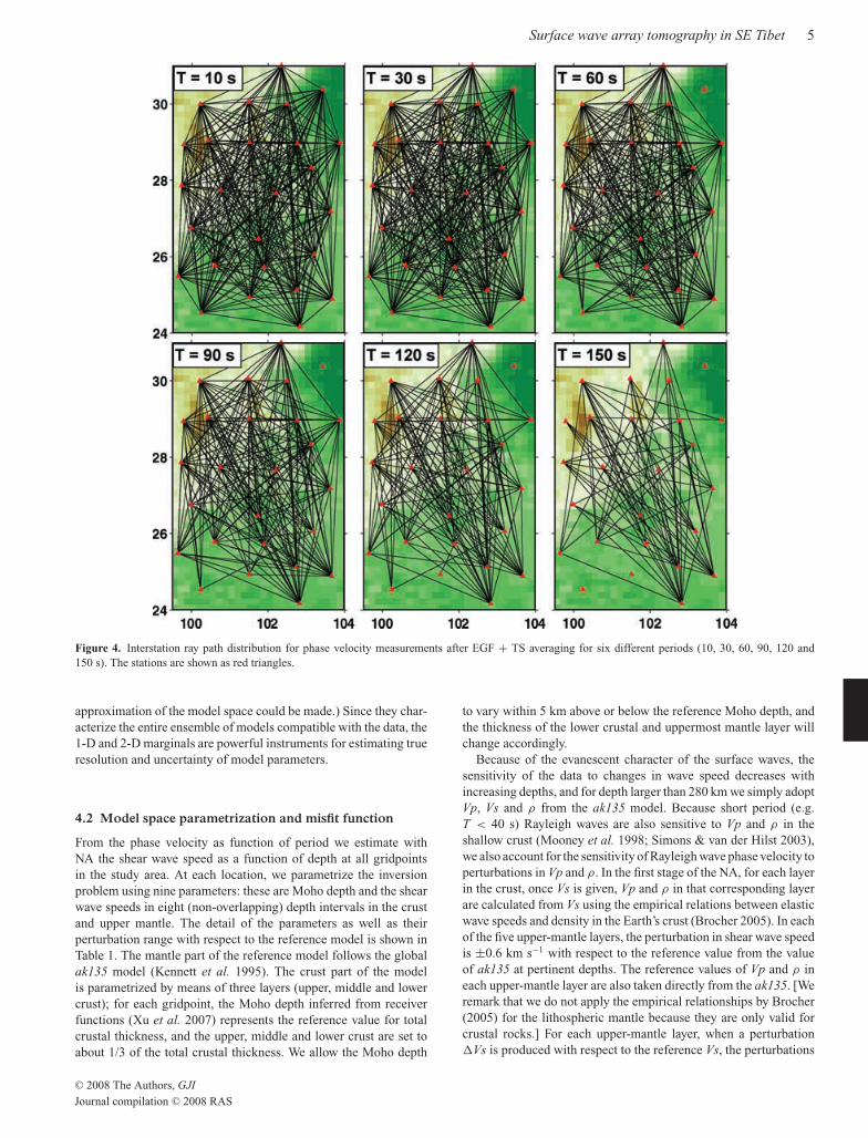
Following Paper I, we construct 2-D phase velocity maps from 10to 150 s. The path distributions for six different periods (10, 30,60, 90, 120 and 150 s) are shown in Fig. 4. At each period the datacoverage is denser than in Paper I, especially at the longer peri-ods. The corresponding phase velocity maps are shown in Fig. 5.

The lateral resolution in these maps is generally of the order of(or less than) the interstation distance (∼100 km). From the maps,we infer the phase velocity as a function of frequency at eachpoint of the 0.5◦ × 0.5◦ grid that is used to parametrize the studyregion.

4 S T RU C T U R E I N V E R S I O N U S I N GN E I G H B O U R H O O D A L G O R I T H M ( N A )

4.1 NA optimization

The NA involves two stages (Sambridge 1999a,b). The first stageconsists of a model space search to identify the ‘good’ data fittingregions. It employs a geometrical construct—the Voronoi cells—todrive the search towards the best data-fitting regions while continu-ing to sample a relatively wide variety of different models. The useof these cells makes this algorithm self-adaptative because, with agood choice of some tuning parameters, one can explore the com-plete model space with the possibility to jump out of a local min-imum. It also has the advantage of being able to sample severalpromising regions simultaneously. During this search, the samplingdensity increases in the surroundings of the good models withoutlosing information on the models previously generated (even the‘bad’ ones). The first stage results in a distribution of misfits, whichserves to approximate the posterior probability density function(PPDF).

In the second stage of NA, a sampling of this distribution gener-ates a ‘resampled ensemble’ that follows the PPDF. This resampledensemble is then integrated numerically to compute the likelihoodassociated with each model parameter, also called 1-D marginalPPDFs (or 1-D marginals), the correlation matrix and 2-D marginalPPDFs (or 2-D marginals). The departure of these 1-D marginalsfrom a Gaussian distribution can be used as a diagnostic of the de-gree of ill-posedness of the problem. In addition, their width canbe seen as a more realistic measure of model uncertainty than onewe obtain from traditional inversion techniques. The 2-D marginalsquantify the trade-offs between two variables. (NB the same infor-mation can be deduced from the correlation matrix if a Gaussian





Figure 4. Interstation ray path distribution for phase velocity measurements after EGF + TS averaging for six different periods (10, 30, 60, 90, 120 and150 s). The stations are shown as red triangles.

approximation of the model space could be made.) Since they char-acterize the entire ensemble of models compatible with the data, the1-D and 2-D marginals are powerful instruments for estimating trueresolution and uncertainty of model parameters.

4.2 Model space parametrization and misfit function

From the phase velocity as function of period we estimate withNA the shear wave speed as a function of depth at all gridpointsin the study area. At each location, we parametrize the inversionproblem using nine parameters: these are Moho depth and the shearwave speeds in eight (non-overlapping) depth intervals in the crustand upper mantle. The detail of the parameters as well as theirperturbation range with respect to the reference model is shown inTable 1. The mantle part of the reference model follows the globalak135 model (Kennett et al. 1995). The crust part of the modelis parametrized by means of three layers (upper, middle and lowercrust); for each gridpoint, the Moho depth inferred from receiverfunctions (Xu et al. 2007) represents the reference value for totalcrustal thickness, and the upper, middle and lower crust are set toabout 1/3 of the total crustal thickness. We allow the Moho depth

to vary within 5 km above or below the reference Moho depth, andthe thickness of the lower crustal and uppermost mantle layer willchange accordingly.

Because of the evanescent character of the surface waves, thesensitivity of the data to changes in wave speed decreases withincreasing depths, and for depth larger than 280 km we simply adoptVp, Vs and ρ from the ak135 model. Because short period (e.g.T < 40 s) Rayleigh waves are also sensitive to Vp and ρ in theshallow crust (Mooney et al. 1998; Simons & van der Hilst 2003),we also account for the sensitivity of Rayleigh wave phase velocity toperturbations in Vp and ρ. In the first stage of the NA, for each layerin the crust, once Vs is given, Vp and ρ in that corresponding layerare calculated from Vs using the empirical relations between elasticwave speeds and density in the Earth’s crust (Brocher 2005). In eachof the five upper-mantle layers, the perturbation in shear wave speedis ±0.6 km s−1 with respect to the reference value from the valueof ak135 at pertinent depths. The reference values of Vp and ρ ineach upper-mantle layer are also taken directly from the ak135. [Weremark that we do not apply the empirical relationships by Brocher(2005) for the lithospheric mantle because they are only valid forcrustal rocks.] For each upper-mantle layer, when a perturbation�Vs is produced with respect to the reference Vs, the perturbations





24

26

28

30

0

2

4

6

100 102 104

100 102 10424

26

28

30

100 102 104

T = 10 s T = 30 s T = 60 s

T = 90 s T = 120 s T = 150 s

Figure 5. Perturbation (in percentage) of 2-D phase velocity maps at 6 different periods (10, 30, 60, 90, 120 and 150 s) with respect to the average phasevelocities (red dots in Fig. 2(b)) constructed from the dispersion data after EGF + TS averaging. The corresponding ray path distribution map at each period isshown in Fig. 4. The stations are shown as black triangles.

Table 1. Model parameters as well as their reference value, perturbation range, and average perturbation in NA.

Name of model parameter Reference value of parameter Perturbation with respect to the reference value Average perturbation

Moho depth H (km) [−5 5] km −0.32 kmVs in the upper crust 3.4 km s−1 [−0.8 0.4] km s−1 −0.069 km s−1

Vs in the middle crust 3.6 km s−1 [−0.8 0.4] km s−1 −0.192 km s−1

Vs in the lower crust 3.8 km s−1 [−0.8 0.4] km s−1 −0.120 km s−1

Vs in Moho – 90 km Vs from ak135 (km s−1) [−0.6 0.6] km s−1 −0.197 km s−1

Vs in 90–130 km Vs from ak135 (km s−1) [−0.6 0.6] km s−1 −0.053 km s−1

Vs in 130–170 km Vs from ak135 (km s−1) [−0.6 0.6] km s−1 0.102 km s−1



H denotes the reference Moho depth from teleseismic receiver functions (Xu et al. 2007) and Vs is shear wave speed (km s−1). ‘Average Perturbation’ in thefourth column means the average perturbation of the model parameters for all gridpoints in the study region. The average Moho depth is 49.87 km fromreceiver functions (Xu et al. 2007) and 49.55 km after NA.

of P-wave speed (�Vp) and density (�ρ) with respect to the ak135values for that layer are also obtained using the following relations(Masters et al. 2000):

d ln Vp

d ln Vs= 0.6,

d ln ρ

d ln Vs= 0.4. (1)

Through the use of relationships among Vs, Vp and ρ for the crustaland mantle layers, we thus incorporate the influence of Vp and ρ onthe phase velocities in NA.

For every model generated in the NA model space search,Rayleigh wave phase velocities are calculated in the period band

10–150 s. To calculate misfit we use the L2-norm to represent thedistance between the predicted and the observed dispersion data

= 1

N

N∑i=1

(cpred

i − cobsi

σ i

)2

1/2

, (2)

where N is the total number of periods at which the phase velocity ismeasured; cpred

i and cobsi is the predicted and observed phase velocity

at the ith period, respectively; σ i is the estimated standard error ofthe observed phase velocity at the ith period. In this study, N = 25,





and σ i is set to be 0.01cobsi because the standard error of intersta-

tion phase velocity measurements is about 1 per cent (Yao et al.2006).

Each stage of the NA requires the tuning of parameters whoseoptimum values have to be found by trial and error. Several authorshave described the influence of these parameters on the survey of themodel space and on the Bayesian interpretation of the results (e.g.Sambridge 1999a,b; Resovsky & Trampert 2002). To broaden thesurvey in the model space and to consider the speed of convergenceof the algorithm, the total number of new models generated at eachiteration step, ns, is set to 100, and the number of best data-fittingcells in which the new models are created, nr, is set to 50 after a setof stability and convergence tests.

4.3 Example of NA optimization

We use the dispersion data, the solid dots with error bars inFig. 6(a), at the gridpoint at (101◦E, 29◦N) to illustrate the perfor-mance of NA. Note that the observed phase velocities in the shortand intermediate period range (10–80 s) are much lower than thosepredicted from the reference model (dashed line in Fig. 6a), whichindicates a possible reduction in seismic wave speeds at the crustaland uppermost mantle depth. A total of 35 200 models were gener-ated during the first stage of the NA to ensure the convergence of thesearch. During the second stage, these models and their misfits wereused to produce 1-D and 2-D marginals (Figs 7 and 8, respectively).The 1-D marginals are used to determine the posterior mean valueand the corresponding standard error of each model parameter. Amost likely (best-fitting) model can be obtained from the peak of the1-D marginal distributions. The posterior mean model is shown asthe solid line in Fig. 6(b) and the corresponding predicted dispersioncurve is shown as the solid line in Fig. 6(a), which falls within datauncertainties.

The width of the 1-D marginal distributions shown in Fig. 7demonstrates that Vs is better constrained in the three crustal layersthan in the upper-mantle layers. The standard errors of Vs associ-ated with the posterior mean model parameters are also shown asthe grey area in Fig. 6(b). The shallow crust can be constrained bet-ter than the lower crust because short-period (dispersion) data hasa narrower depth sensitivity kernel and, in particular, because thewave speed estimates for the lower crust structure trade-off stronglywith the Moho depth. For this gridpoint the Moho depth is poorlyconstrained. The posterior mean Moho depth is 57.8 km with a stan-dard error about 3 km. The posterior mean shear wave speeds (solidlines in Fig. 7) of the three crustal layers are very close to the mostlikely model, the peak of the corresponding 1-D marginals with ap-proximate Gaussian distributions. For the five upper-mantle layers,the posterior mean shear wave speeds are also close to the mostlikely model, but generally with larger standard errors than those ofthe crustal layers, indicating that the long-period surface data whichsample this depth range have relatively poorer depth resolution. TheVs of uppermost mantle layer (Moho—90 km) has the largest stan-dard error (0.29 km s−1), implying a large trade-off between Mohodepth and the shear wave speed. The posterior mean shear wavespeeds of both the middle crust and the lower crust are much lowerthan the Vs in the reference model (Figs 6b and 7). Relatively lowshear wave speed also persists in one of the upper-mantle layer (90–130 km). However, from 130 to 280 km, the posterior mean Vs ishigher than that of ak135.

The 2-D marginals (Fig. 8) illustrate the trade-off between dif-ferent model parameters. The Vs in nearby layers shows apparent

20 40 60 80 100 120 140

3

3.2

3.4

3.6

3.8

4

4.2

4.4

Period (sec)

Ph

ase

Vel

oci

ty (

km/s

)

ObservationPosterior Mean ModelReference Model

3 3.5 4 4.5 50

40

80

120

160

200

240

280

Shear Wavespeed (km/s)

Dep

th (

km)

Posterior Mean ModelReference Model

a

b

Figure 6. Rayleigh-wave phase velocity dispersion curves (a) and shearwave speed model (b) for the gridpoint at (101◦E, 29◦N) obtained fromthe NA. The observed dispersion data at the gridpoint are shown as theblack dots in (a). The error bar on the observed dispersion point shows thestandard error (1 per cent of the observed phase velocity) of the dispersionmeasurement at each period. The solid line in (b) shows the posterior meanVs model and the predicted dispersion curve from this model is shown asthe solid line in (a). The dashed line in (a) shows the predicted dispersioncurve of the reference model [the dashed line in (b)], which consists of threecrustal layers and mantle structure from the global ak135 model (Table 1).The width of the shaded area shows the standard error of the posterior meanVs in each layer.

negative correlations. The trade-off between Vs of adjacent layersin the crust is smaller compared to trade-offs between Vs in nearbyupper-mantle layers. This is a reflection of the fact that depth res-olution is better for shorter than for longer period dispersion data.The Moho depth shows large trade-off (positive correlation) withthe Vs in the lower crust and that in the uppermost mantle (Moho—90 km) (Fig. 8). Indeed, Moho depth cannot be constrained wellwith dispersion data alone because of the trade-off between theMoho depth and the wave speeds in the lower crust and uppermostmantle (Fig. 8). We recall, however, that we use the Moho depthsfrom receiver function studies (Xu et al. 2007) as reference valuesin the NA search, which results in better estimations of the Mohodepth than from dispersion data alone.





moho depth (km) ∆Vs: upper crust6053 55 63

∆Vs: middle crust

∆Vs: lower crust ∆Vs: Moho-90 km ∆Vs: 90-130 km

∆Vs:130-170 km ∆Vs: 170-220 km ∆Vs: 220-280 km

0 0.4-0.4-0.8 0 0.4-0.4-0.8

0 0.4-0.4-0.8 0-0.6 0.60.3-0.3 0-0.6 0.60.3-0.3

0-0.6 0.60.3-0.3 0-0.6 0.60.3-0.3 0-0.6 0.60.3-0.3

Figure 7. 1-D marginal posterior probability density functions (PPDFs) of the nine model parameters at (101◦E, 29◦N). The horizontal axis shows the variationrange of Moho depth (km) or the perturbation range of �Vs (km s−1) for each layer as shown in Table 1 and the vertical axis is the normalized posteriorprobability density. In each plot, the solid line shows the parameter value of the posterior mean model. The reference Moho depth for this gridpoint is 58 km,and the posterior mean value from of the Moho depth from the 1-D marginal is 57.8 km with a standard error about 3 km. The almost flat 1-D marginal PPDFof the Moho depth implies the Moho depth is not well constrained at this gridpoint. Note that the posterior mean �Vs of each crustal layer is very close to thevalue of the most likely model, which corresponds to the peak of each 1-D marginal PPDF with almost Gaussian distribution.

5 C RU S TA L A N D U P P E R - M A N T L ES T RU C T U R E

From the 1-D posterior mean model and standard error inferredfrom the NA at each gridpoint, we infer 3-D wave speed variations,and their uncertainty, beneath the array. We will now present theinferred variation in Moho depth and images of Vs variations atdifferent depths and along different vertical profiles.

5.1 Variation of Moho depth

In map view, the lateral variation in Moho depth beneath the arrayarea is presented in Fig. 9. These results are, by design, consistentwith the estimates by Xu et al. (2007). From west to east across thearray the Moho depth decreases rather abruptly from 55–63 km insouthwest Sichuan (i.e. the northwestern part of the array) to 37–45 km beneath the western margin of Sichuan basin. Southeastwardthe Moho depth (and crustal thickness) decreases more gradually to∼40 km beneath central Yunnan. The 1-D marginals suggest thatthe standard error in Moho depth is 2–3 km.

5.2 3-D variation in shear wave speed

The lateral variation of Vs at 10, 25, 50, 75, 100 and 200 km depthis depicted in Fig. 10, with the uncertainties displayed in Fig. 11.Fig. 12 shows Vs heterogeneity along five vertical profiles from thesurface to 250 km depth, with the uncertainties shown in Fig. 13.

In the Chuan-Dian Fragment (Fig. 1b, the magenta shaded area)the wave speed patterns vary significantly from the upper crust tothe upper mantle. In the upper crust, high wave speed appears inthe central and eastern part of this tectonic unit, while low wavespeed mainly appears in the southern and western parts (Fig. 10a).The region northeast of the Red River fault (only the northern partis sampled in this study) shows prominent low wave speed in theupper crust (Fig. 10a), but this feature seems to disappear at largerdepths. At the mid-crustal depth range, the northern Chuan-DianFragment is marked by a LVL, bounded to the south approximatelyby the Lijiang and Muli faults (Fig. 10b). Another prominent mid-crustal LVL appears in the southeastern part of Chuan-Dian Frag-ment, around the Luzhijiang-Xiaojiang fault zone (Fig. 10b; profilesCC′ and DD′ in Fig. 12). In the lower crust, a LVL appears in the





Figure 8. Examples of 2-D marginal PPDFs of the nine model parameters at (101◦E, 29◦N). In each panel, the values for the horizontal and vertical axis showthe perturbation range of �Vs (km s−1) for each layer or the variation range of Moho depth (km). Black, blue and red lines are the contours to show 60, 90 and99 per cent confidence level. The more circular and narrower the contour is, the smaller the trade-off between the two model parameters is. The posterior meanmodel is shown as a green triangle in each plot.

central part of Chuan-Dian Fragment, and in contrast to the middlecrust the lower crust beneath northern portion is not anomalouslyslow (Fig. 10c; profiles AA′, BB′ and EE′ in Fig. 12). We note alsothat the LVL detected at mid-crustal depth beneath the northernChuan-Dian Fragment (Fig. 10b) does not extend northeastwardacross the Xianshuihe fault (XSHF); in fact, normal shear wavespeeds are observed northeast of this fault (profile AA′ in Fig. 12).

In the uppermost mantle (Fig. 10d), the eastern Chuan-Dian Frag-ment mainly appears slow while relatively high wave speeds prevailin part of the central fragment north of Lijiang fault. At 100 km depth(Fig. 10e), the northern Chuan-Dian Fragment is marked by lowwave speeds while southern Chuan-Dian Fragment is relatively fast.The wave speed pattern at 200 km depth beneath the Chuan-DianFragment (Fig. 10f) seems to be quite different from that at 100 kmdepth, with low wave speed anomaly in the south fragment but highvelocity anomaly in the northern fragment.

At very shallow depths, shear wave speed is slow in the westernmargin of Sichuan basin (Fig. 10a), probably due to presence of thethick sedimentary layers, but wave speed is high in the middle crust(Fig. 10b). The upper-mantle structure below the western margin ofthe Sichuan basin may be not reliable because the path coverage atintermediate and longer periods is poor (Fig. 4). Southwest of theZhongdian–Dali–Red River fault the uppermost mantle (Moho—130 km) is relatively slow (Figs 10d and e), while at 200 km depthit changes to fast structure (Fig. 10f).

The average wave speeds in each layer of the study region areshown in Table 1. With respect to the reference value, we observe

relatively low wave speeds in the three crustal layers and two up-permost mantle layers (Moho—90 km, 90–130 km) and higherwave speeds in other three deeper upper-mantle layers (130–170,170–220 and 220–280 km). The average crustal velocity is about3.47 km s−1, which is about 4.3 per cent lower than that(∼3.63 km s−1) of the global ak135 (continental) crustal model.

6 D I S C U S S I O N

The variation of the 3-D shear wave speed structure in the crustand upper mantle beneath the array area (up to about ±8 per centvariation with respect to the average value) is much larger than sug-gested by traditional (larger scale, but lower resolution) surface wavetomography. The inferred heterogeneity reflects a complicated (tec-tonic) transition from the Tibetan Plateau (Lhasa block, Qiangtangblock and Songpan-Ganze Fold Belt) to the South China Block andIndo-China Block. Our results suggest that boundaries between ma-jor tectonic units identified at the surface appear to involve much—ifnot all—of the crust, and in some cases the uppermost mantle aswell.

6.1 Uncertainties of the shear wave speeds from NA

Fig. 11 shows the standard errors (or uncertainties) of shear wavespeeds for horizontal profiles at different depths in Fig. 10, andFig. 13 shows the standard errors of shear wave speeds for vertical





Figure 9. Variation of the Moho depth as inferred from the posterior meanmodel using the NA at each gridpoint in the studied area. The colour bar inthe right corner shows the value of Moho depth. The black thick lines are thesection lines of the vertical profiles (AA′, BB′, CC′, DD′ and EE′) shown inFig. 12.

profiles in Fig. 12. The standard errors in the shear wave speed esti-mates are relatively small (∼0.15–0.2 km s−1) at upper and middlecrustal depth but larger (∼0.2–0.3 km s−1) in the lower crust and theupper-mantle layers (Figs 11 and 13). This is due to the trade-offswith Moho depth and to the evanescent properties of surface wavesat different periods: shorter period surface waves have a better depthsensitivity in the shallow crust, whereas longer period surface wavessample the upper-mantle structure with a much broader depth sen-sitivity kernel which results in a relatively poor depth resolution inthe upper mantle.

At a given depth, the standard errors vary laterally (Figs 11 and13) because of the lateral variability in model parametrization of thecrust and upper-mantle layers (Section 4.2) and lateral variations instandard error of phase velocity. Estimating the uncertainties onthe 2-D phase velocity maps directly from the uncertainties on theinterstation measurements is still difficult at this stage. This is whywe made a rough estimate using 1 per cent of the phase velocitydetermined at every period for each gridpoint.

The wave speed error is generally inversely proportional tolayer thickness. For example, in the uppermost mantle layer(Moho—90 km) the largest uncertainties occur in regions where theMoho is deepest and, hence, the layer thinnest [i.e. in the northwest-ern part of the study region (Figs 9 and 11d)]. Setting the thicknessof the upper and middle crust layer both about 1/3 of the total crustalthickness prevents any of these layers to become arbitrarily thin. Thewave speed uncertainty is generally larger in the lower crust than in

the upper and middle crust (Figs 11 and 13) because of the reducedsensitivity of the data and also because of the trade-off betweenMoho depth and the wave speed of the lower crust.

The uncertainty maps suggest that the LVLs in the middlecrust, for example, in the northern Chuan-Dian Fragment and theLuzhijiang-Xiaojiang fault zone, are robust. Also the LVL in thelower crust beneath the central Chuan-Dian Fragment seems tobe well resolved (Figs 13b, c and e). Some of the structures inthe upper mantle have larger uncertainties. Because we performed amodel space search that provided PPDFs for each model parameter,we have an overview of all the models compatible with the data.We did not choose a particular model based on regularization, as wewould with a more traditional inverse method. In addition, becausewe carefully sampled the model space (with appropriate choice ofthe tuning parameters to make a broad sampling), we are confidentthat the models we obtained are not associated with local minimaof the misfit function.

6.2 Heterogeneity of Chuan-Dian Fragment

The Chuan-Dian Fragment is usually regarded as a unique tectonicterrane and is thought to play an important role in the dynamics andtectonics of the eastern part of the Tibetan Plateau. According torecent GPS studies (King et al. 1997; Chen et al. 2000; Zhang et al.2004; Shen et al. 2005) this block is moving southeastward at a ratelarger than adjacent crust, which indicates that the crustal materialis transported from the central part of the Tibetan Plateau to SWChina and Burma around the EHS by clockwise rotation. However,the Chuan-Dian Fragment is not tectonically uniform, and on thebasis of geological and geodetic studies one can identify differenttectonic units (Wang et al. 1998; Wang & Burchfiel 2000; Shen et al.2005).

Our results confirm that the crust and upper mantle beneath theChuan-Dian Fragment are highly heterogeneous. At the surface, theXianshuihe-Xiaojiang left-lateral fault system acts as the bound-ary between the Chuan-Dian Fragment and the South China block(which comprises the Yangtze Craton and the South China FoldBelt). In the northern part of the study region, we observe largewave speed contrasts across the Xianshuihe fault at the mid-crustaldepth (Fig. 10b). Further south, and at larger depths, the Xiaojiangfault is not evident in the images. Further study must establish ifthis is a resolution issue or if it reflects spatial variations in char-acter of and elastic properties across the fault. The data also revealsubstantial contrasts across the Lijiang-Muli fault system (Fig. 10),which suggests that it is a main boundary within the Chuan-DianFragment. This inference is consistent with results from (surface)block modelling using GPS data (Shen et al. 2005), which identifiesa northern block (including the Yajiang and Shangrilla subblocks)and a southern block (the Central Yunnan subblocks), separated bythe Lijiang-Muli fault. The Lijiang-Muli fault is also part of theboundary between the Songpan-Ganza Fold Belt and the YangtzeCraton (Fig. 1b).

6.3 Crustal weak zones and the importance of faults

The tomographic images of the continental lithosphere demonstratethat LVLs are ubiquitous in the middle/lower crust and upper mantlebeneath the southeastern borderland of the Tibetan Plateau. This isconsistent with previous results (e.g. Huang et al. 2002; Wang et al.2003; Hu et al. 2005a,b; Xu et al. 2007), but because of superior





Figure 10. Variation in shear wave speed relative to the posterior mean model inferred from the NA: (a) 10 km; (b) 25 km; (c) 50 km; (d) 75 km; (e) 100 kmand (f) 200 km. The major faults are depicted as thin black lines – for abbreviations see Fig. 1(b). The thick dark green lines are the block boundaries from thesurface GPS data modelling (Shen et al. 2005). The abbreviations for subblocks are YJ (Yajiang), SH (Shangrilla), CY (Central Yunnan), LMS (Longmenshan)and BS (Baoshan) subblock (S-B). The white lines in (c) are the contour lines of Moho depth and the values are shown as the black numbers on them. Thecolour bar in the right corner of each plot shows the value of shear wave speed (km s−1).

depth resolution we can determine, more confidently, the depth andlateral continuity of these LVLs.

High regional surface heat flow values (Hu et al. 2000) indicatesteep geothermal gradients. The high geothermal gradient can re-duce the shear wave speed and may cause partial melt in the crust.Partial melt of the crustal material in the Tibetan Plateau has beensuggested by other studies, for example, partially molten in the mid-dle crust beneath southern Tibet (Nelson et al. 1996; Unsworth et al.2005), and in the mid-lower crust and upper mantle beneath northernTibet (Meissner et al. 2004; Wei et al. 2001). It thus seems reasonableto attribute the large (>10 per cent), local reductions in shear wavespeed to a reduction in rigidity due to elevated temperatures and,perhaps, partial melt in the middle or lower crust. Even small meltfractions would reduce the strength of the lithosphere (Kohlstedt& Zimmerman 1996) and facilitate intracrustal (plastic) flow dueto external tectonic forces. From analysis of seismic anisotropy,Shapiro et al. (2004) and Ozacar & Zandt (2004) argued that chan-nel flow is likely within the middle or middle-to-lower crust beneaththe central parts of the plateau. The argument of crustal channel flowis further supported by the very low equivalent elastic thickness (0< Te < 20 km) beneath the Tibetan Plateau and SW China (Jordan& Watts 2005), and by the detection of zones of high (electric) con-ductivity in the crust of our study region (Sun et al. 2003; Bai et al.2006).

The presence (or absence) of weak zones is important for our un-derstanding of the geological development of the Tibetan Plateau.Indeed, geodynamic modelling involving gravity and/or thermaldriven lateral flow within a weak middle/lower crust channel hasbeen used to explain the tectonics in the Himalayan–Tibetan oro-gen (e.g. Beaumont et al. 2004) and eastern Tibet (e.g. Roydenet al. 1997; Clark & Royden 2000; Shen et al. 2001). But manyfirst-order issues about such weak layers have remained unresolved.The (geographical and depth) distribution of and interconnectivitybetween LVLs—and, by implication, the 3-D geometry of the pre-sumed channel flow—are not well known. Can flow occur freelyover large regions or are there local structures (such as faults) thatinterrupt or deflect flow? And what is effect of the asthenosphericupper mantle on crustal channel flow? Answering these questionswill be of key importance for understanding the (tectonic) blockmotions inferred from GPS data and—indeed—regional seismicity.

In northern Tibet, the possible weak channel due to partial meltis likely to exist from the middle crust to upper mantle (Meissneret al. 2004; Wei et al. 2001). In southern Tibet, beneath the Hi-malayan orogen, many geophysical observations (e.g. Nelson et al.1996; Unsworth et al. 2005) suggest that the partial melt andthe consequent weaker channel probably dominate in the mid-dle crust. In southeastern Tibet, lower crustal flow models (e.g.Royden et al. 1997) explain many geological aspects, such as





σV (km/s)

0.16

0.18

0.20

0.22

0.24

0.26

0.28

0.30

0.15

24

25

26

27

28

29

30

3110 km

a b

25 km

c

50 km

100 101 102 103 10424

25

26

27

28

29

30

31

d

75 km

100 101 102 103 104e

100 km

100 101 102 103 104f

200 km

Figure 11. Standard error (σ v) of the shear wave speed at different depths shown in Fig. 10. The colour bar in the right shows the value of σ v (km s−1).

the lack of young crustal shortening and the gentle topographicslope.

Our high-resolution surface wave array tomography reveals con-siderable regional variations in the strength and depth range ofLVLs. In the northern part of the Chuan-Dian fragment and theLuzhijiang-Xiaojiang fault zone, the images reveal a mid-crustalLVL with a (horizontal) E-W extent of 150–200 km. In the centralChuan-Dian Fragment, the data require LVL in the lower crust. Thehigh-resolution (3-D) images are beginning to suggest that some ma-jor fault zones in this area (e.g. Xianshuihe fault, Litang fault andLuzhijiang fault) mark lateral transitions in the mid- or lower crustalLVZs. This crustal heterogeneity implies that the flow pattern is morecomplicated and, in particular, that some of the major faults seem toplay a more important role than assumed in the current generationof middle or lower crustal flow models. A better understanding ofthese structural relationships requires even higher resolution imagesof the crust beneath this region. This can be achieved through a com-bination of denser array deployments and the use of more powerfulinverse scattering or (full wave) inversion approaches (e.g. De Hoopet al. 2006).

7 S U M M A RY

We have used dispersion data from EGF and TS analysis to con-struct high-resolution Rayleigh wave phase velocity maps in theperiod band 10–150 s in the southeastern borderland of the TibetanPlateau. These phase velocity maps were then inverted for 3-D shearwave speed variations in the study region using the NA. With NA,

a global optimization method, we estimated parameter trade-offsand uncertainties. Because of the large trade-off between the Mohodepth and the shear wave speed in the lower crust and uppermostmantle, we constrain the Moho depth using results from receiverfunction studies (Xu et al. 2007). The 15 per cent peak-to-peakvariation of shear wave speed implies a complicated tectonic makeup of the southeastern borderland of the Tibetan Plateau. The shearwave speed in the shallow crust beneath Chuan-Dian Fragment ischaracterized by regions with high and low velocity anomaly sep-arated by some of the major faults, which is consistent with thetectonic and GPS studies and implies that Chuan-Dian Fragment isnot a uniformly rigid block. Prominent LVLs have been found inthe middle crust beneath the northern Chuan-Dian Fragment andthe Luzhijiang-Xiaojiang fault zone and in the lower crust beneaththe central Chuan-Dian Fragment.

The high-resolution images are beginning to reveal relationshipsbetween major faults in the area and the occurrence and lateral ex-tent of crustal LVLs. The heterogeneous spatial distribution of theLVLs in the middle or lower crust in the southeastern borderland ofthe Tibetan Plateau and the possible interaction of the major faultswith deep crustal structure suggest that the pattern of the possiblecrustal channel flow is complicated and may involve both middleand lower crustal flow. Establishing the relationship between majorfault systems and the spatial distribution of crustal weak zones is ofkey importance for our understanding of the regional block motion(as inferred from GPS) and seismicity. These structural relation-ships are not yet fully resolved with the data coverage and inversiontechniques used here, but we anticipate that new array deployments





Figure 12. Shear wave speed variation relative to the posterior mean model inferred from the NA along five vertical profiles (AA′, BB′, CC′, DD′ and EE′shown in the bottom of each plot; for location, see Fig. 9). The wave speed (km s−1) colour scale is shown in the right. Topography is depicted above eachprofile (black area) and the arrows above it mark the location of major faults along each profile. The abbreviations for fault names are the same as in Fig. 1(b).The black line (around 50 km depth) on each colour profile indicates the Moho discontinuity.

and the use of more powerful combinations of interferometry andfull wave inversion methods will change this situation in the not toodistant future.

A C K N O W L E D G M E N T S

We thank the Editor Jeannot Trampert and two anonymous review-ers for their constructive comments, which helped us improve themanuscript. We also thank Dr Malcolm Sambridge for providingus the source code of the NA, Prof Denghai Bai at the Institute ofGeology and Geophysics Chinese Academy of Science and Jiangn-ing Lu at MIT for sharing their results for comparison, Prof Qiyuan

Liu at Chinese Earthquake Administration for helpful discussionsand Dr Yaoqiang Wu and his research staff at Sichuan EarthquakeAdministration, China for their discussions and hospitality duringour visit to Chengdu, China. This work was supported by the Con-tinental Dynamics Program of the US National Science Foundationunder grant 6892042.

R E F E R E N C E S

Bai, D., Meju, M., Arora, B., Ma, X., Jiang, C., Zhou, Z., Zhao, C., Wang,L., 2006. Large crustal-mantle channel flow in central Tibet and easternHimalaya inferred from magnetotelluric models, Eos Trans. AGU, 87(36),West. Pac. Geophys. Meet. Suppl., Abstract S45A-07.





Figure 13. Standard error (σ v) of the shear wave speed along five vertical profiles shown in Fig. 12. The colour bar in the right shows the value of σ v

(km s−1).

Beaumont, C., Jamieson, R.A., Nguyen, M.H. & Medvedev, S., 2004. Crustalchannel flow: 1. Numerical models with applications to the tectonics of theHimalayan-Tibetan orogen, J. geophys. Res., 109, B06406, doi:10.1029/2003JB002809.

Beghein, C., Resovsky, J.S. & Trampert, J., 2002. P and S tomography usingnormal-mode and surface wave data with a neighbourhood algorithm,Geophys. J. Int., 149, 646–658.

Brocher, T.M., 2005. Empirical relations between elastic wavespeedsand density in the Earth’s crust, Bull. seism. Soc. Am., 95(6), 2081–2092.

Chen, Z. et al., 2000. Global positioning system measurements from easternTibet and their implications for India/Eurasia intercontinental deforma-tion, J. geophys. Res, 105, 16 215–16 227.

Clark, M. & Royden, L.H., 2000. Topographic ooze: building the easternmargin of Tibet by lower crustal flow, Geology, 28(8), 703–706.

De Hoop, M.V., van der Hilst, R.D., Shen, P., 2006. Wave-equation reflectiontomography: annihilators and sensitivity kernels, Geophys. J. Int., 167,1211–1214.

Hu, S., He, L. & Wang, J., 2000. Heat flow in the continental area of China:a new data set, Earth planet. Sci. Lett., 179, 407–419.

Hu, J.F., Su, Y.J., Zhu, X.G. & Chen, Y., 2005a. S-wave velocity and Poisson’sratio structure of crust in Yunnan and its application (in Chinese), Sci.China Ser. D., 48(2), 210–218.

Hu, J.F., Chu, X.G., Xia, J.Y. & Chen, Y., 2005b. Using surface wave andreceiver function to jointly inverse the crust-mantle velocity structurein the West Yunnan area (in Chinese), Chin. J. Geophys., 48(5), 1069–1076.

Huang, J., Zhao, D. & Zheng, S., 2002. Lithospheric structure and its rela-tionship to seismic and volcanic activity in southwest China, J. geophys.Res., 107(B10), 2255, doi:10.1029/2000JB000137.





Jordan, T.A. & Watts, A.B., 2005. Gravity anomalies, flexure and the elasticthickness structure of the India-Eurasia collisional system, Earth planet.Sci. Lett., 236, 732–750.

Kan, R., 1977. Study on the current tectonic stress field and the characteristicsof current tectonics activity in southwest China (in Chinese), Chin. J.Geophys., 20(2), 96–107.

Kennett, B.L.N., Engdahl, E.R. & Buland, R., 1995. Constraints on the veloc-ity structure in the earth from travel times, Geophys. J. Int., 122, 108–124.

King, R.W. et al., 1997. Geodetic measurement of crustal motion in south-west China, Geology, 25, 179–182.

Kohlstedt, D.L. & Zimmerman, M.E., 1996. Rheology of partially moltenmantle rocks, Annu. Rev. Earth planet. Sci., 24, 41–62.

Lev, E., Long, M.D., Van der Hilst, R.D., 2006. Seismic anisotropy in easternTibet from shear wave splitting reveals changes in lithospheric deforma-tion, Earth planet. Sci. Lett., 251, 293–304.

Li, Z.X., 1998. Tectonic history of the major East Asian lithosphere blockssince the mid-Proterozoic. in Mantle Dynamics and Plate Interactions inEast Asia, pp. 211–243, ed. Flower, M. F. J., Chung, S.-L., Lo, C.-H., Lee,T.-Y. Geodyn. Ser., 27.

Li, C., Van der Hilst, R.D. & Toksoz, M.N., 2006. Constraining P-wavevelocity variations in upper mantle beneath Southeast Asia, Phys. Earthplanet. Inter., 154, 180–195.

Li, C., Van der Hilst, R.D., Meltzer, A.S., Sun, R. & Engdahl, E.R., 2008.Subduction of the Indian lithosphere beneath the Tibetan Plateau andBurma, Earth Planet. Sci. Lett., submitted.

Lin, F.-C., Ritzwoller, M.H., Townend, J., Bannister, S. & Savage, M.K.,2007. Ambient noise Rayleigh wave tomography of New Zealand, Geo-phys. J. Int., 170(2), 649–666. doi:10.1111/j.1365–246X.2007.03414.x

Masters, G., Laske, G., Bolton, H. & Dziewonski, A., 2000. The relativebehavior of shear velocity, bulk sound speed, and compressional velocityin the mantle: implications for chemical and thermal structure, Geophys.Monogr. Ser., 117, 63–87.

Meissner, R., Tilmann, F. & Haines, S., 2004. About the lithospheric structureof central Tibet, based on seismic data from the INDEPTH III profile,Tectonophysics, 380, 1–25.

Molnar, P. & Tapponnier, P., 1975. Cenozoic tectonics of Asia: effects of acontinental collision, Science, 189, 419–426.

Mooney, W.D., Laske, G. & Masters, G., 1998. CRUST5.1: a global crustalmodel at 5◦ × 5◦, J. geophys. Res., 103, 727–747.

Nelson, K.D., Zhao, W. J., Brown, L. D., Kuo, J., Che, J., Liu, X., Klemperer,S. L. & Makovsky, Y., 1996. Partially molten middle crust beneath South-ern Tibet: synthesis of Project INDEPTH results, Science, 294, 1684–1688.

Nolet, G., 1985. Solving or resolving inadequate and noisy tomographicsystems, J. Comput. Phys., 61, 463–482.

Ozacar, A. & Zandt, G., 2004. Crustal seismic anisotropy in central Tibet:implications for deformational style and flow in the crust, Geophys. Res.Lett., 31, L23601, doi:10.1029/2004GL021096.

Resovsky, J.S. & Trampert, J., 2002. Reliable mantle density error bars: anapplication of the neighbourhood algorithm to normal-mode and surfacewave data, Geophys. J. Int., 150, 665–672.

Rowley, D.B., 1996. Age of initiation of collision between India and Asia:a review of stratigraphic data, Earth planet. Sci. Lett., 145, 1–13.

Royden, L.H., Burchfiel, B. C., King, R. W., Wang, E., Chen, Z., Shen, F.& Liu, Y., 1997. Surface deformation and lower crustal flow in easternTibet, Science, 276, 788–790.

Sabra, K.G., Gerstoft, P., Roux, P. & Kuperman, W.A., 2005. Surface wave to-mography from microseisms in Southern California, Geophys. Res. Lett.,32, L14311, doi:10.1029/2005GL023155.

Sambridge, M., 1999a. Geophysical inversion with a neighbourhood algo-rithm – I. Searching a parameter space, Geophys. J. Int., 138, 479–494.

Sambridge, M., 1999b. Geophysical inversion with a neighbourhood algo-rithm – II. Appraising the ensemble, Geophys. J. Int., 138, 727–746.

Shapiro, N.M., Campillo, M., Stehly, L. & Ritzwoller, M.H., 2005. High-resolution surface wave tomography from ambient seismic noise, Science,307, 1615–1618.

Shen, F., Royden, L.H. & Burchfiel, B.C., 2001. Large-scale crustal defor-mation of the Tibetan Plateau, J. geophys. Res., 106(B4), 6793–6816.

Shen, Z.-K., Lu, J., Wang, M. & Burgmann, R., 2005. Contemporary crustaldeformation around the southeast borderland of the Tibetan Plateau, J.geophys. Res., 110, B11409, doi:10.1029/2004JB003421.

Simons, F.J. & Van der Hilst, R.D., 2003. Structure and deformation of theAustralian lithosphere, Earth planet. Sci. Lett., 211, 271–286.

Snoke, J.A. & Sambridge, M., 2002. Constraints on the S-wave velocitystructure in a continental shield from surface-wave data: comparing lin-earized least-squares inversion and the direct-search neighbourhood al-gorithm, J. geophys. Res., 107(B5), 2094, doi:10.1029/2001JB000498.

Sol, S. et al., 2007. Geodynamics of southeastern Tibet from seismicanisotropy and geodesy, Geology, 35, 563–566, doi:10.1130/G23408A.1.

Sun, J., Jin, G.W., Bai, D.H. & Wang, L.F., 2003. Electrical structureof the crust and upper mantle and tectonics sense on the edge of theEast Tibet, Science in China (Series D) (in Chinese), 33 (Suppl.) 173–180.

Tapponnier, P., Xu, Z., Roger, F., Meyer, B., Arnaud, N., Wittlinger, G. &Yang, J., 2001. Oblique stepwise rise and growth of the Tibet Plateau,Science, 294, 1671–1677.

Unsworth, M.J., Jones, A.G., Wei, W., Marquis, G., Gokarn, S.G. & Spratt,J.E., 2005. Crustal rheology of the Himalaya and southern Tibet frommagnetotelluric data, Nature, 438, 78–81.

Wang, E. & Burchfiel, B.C., 2000. Late Cenozoic to Holocene deformationin southwestern Sichuan and adjacent Yunnan, China, and its role in for-mation of the southeastern part of the Tibetan Plateau, Geol. Soc. Am.Bull., 112, 413–423.

Wang, E., Burchfiel, B.C., Royden, L.H., Chen, L., Chen, J., Li, W. & Chen,Z., 1998. Late Cenozoic Xianshuihe-Xiaojiang, Red River and Dali faultsystems of southwestern Sichuan and central Yunnan, China, Spec. Pap.Geol. Soc. Am., 327, 1–108.

Wang, C.-Y., Chan, W.W. & Mooney, W.D., 2003. Three-dimensional ve-locity structure of crust and upper mantle in southwestern China andits tectonic implications, J. geophys. Res., 108(B9), 2442, 176–193,doi:10.1029/2002JB001973.

Wei, W. et al., 2001. Detection of widespread fluids in the Tibetan crust bymagnetotelluric studies, Science, 292, 716–718.

Xu, L., Rondenay, S., Van der Hilst, R.D., 2007. Structure of the crust be-neath the Southeastern Tibetan Plateau from teleseismic receiver func-tions, Phys. Earth Planet. Int., doi:10.1016/j.pepi.2007.09.002.

Yang, Y., Ritzwoller, M.H., Levshin, A.L. & Shapiro, N.M., 2007. Ambientnoise Rayleigh wave tomography across Europe, Geophys. J. Int., 168,259–274.

Yao, H., Van der Hilst, R.D. & de Hoop, M.V., 2006. Surface-wave ar-ray tomography in SE Tibet from ambient seismic noise and two-stationanalysis—I. Phase velocity maps, Geophys. J. Int., 166, 732–744.

Yoshizawa, K. & Kennett, B.L.N., 2002. Non-linear waveform inversionfor surface waves with a neighbourhood algorithm—application to mul-timode dispersion measurements, Geophys. J. Int., 149, 118–133.

Zhang, P. et al., 2004. Continuous deformation of the Tibetan Plateau fromglobal positioning system data, Geology, 32(9), 809–812.

Zhang, Z., Bai, Z., Wang, C., Teng, J., Lu, Q., Li, J., Sun, S & Wang, Z.,2005. Crustal structure of Gondwana- and Yangtze-typed blocks: an ex-ample by wide-angle seismic profile from Menglian to Malong in west-ern Yunnan, Science in China (Series D) (in Chinese), 48(11), 1826–1836.



surface wave array tomography in se tibet from …cbeghein/pdfs/2008_yao_etal_gji.pdf ·...

Documents