surface pasteurisation of food packages by the inversion...
TRANSCRIPT

SURFACE PASTEURISATION OF FOOD
PACKAGES BY THE INVERSION
METHOD
by
FLORA P. CHALLOU
A thesis submitted to
The University of Birmingham
for the degree of
DOCTOR OF PHILOSOPHY
School of Chemical Engineering
College of Engineering and Physical
Sciences
The University of Birmingham
January 2016

University of Birmingham Research Archive
e-theses repository This unpublished thesis/dissertation is copyright of the author and/or third parties. The intellectual property rights of the author or third parties in respect of this work are as defined by The Copyright Designs and Patents Act 1988 or as modified by any successor legislation. Any use made of information contained in this thesis/dissertation must be in accordance with that legislation and must be properly acknowledged. Further distribution or reproduction in any format is prohibited without the permission of the copyright holder.
Abstract
- i
Abstract
Thermal processing is the most widely used and well established preservation method used in
the food industry for ensuring food safety and extending the shelf life of food products.
Besides from the food product, the package needs also to be decontaminated to achieve the
required safety goals. This research is concerned with surface pasteurisation treatments in
food packages by the method of inversion, primarily for hot-filled food products. Starch
solutions and tomato soup, used as model fluids in the current work, were hot-filled in glass
jars, were sealed and then inverted for thirty seconds at a filling temperature of 80oC for
achieving a target process equivalent of 5 min at 70oC; the inversion step was used as a
thermal treatment of the headspace and the lid. The inverted jars showed significantly higher
process values for the headspace and the lid with the filling temperature being the most
important parameter.
The effectiveness of the inversion step during hot-fill treatments was quantified by the use of
two monitoring techniques, the traditional temperature sensors and the alternative, enzymic
based (Bacillus amyloliquefaciens α-amylase) Time Temperature Integrators (TTIs). TTIs are
small devices with kinetics similar to the microorganisms, whose level of degradation is
measured at the end of the thermal process. The enzyme activity obtained is integrated and the
temperature history can be quantified. TTIs were tested for their reliability and accuracy
under isothermal and non-isothermal conditions, and were then used for validating the hot-fill
process.
The behaviour of the model fluids was investigated by performing rheological analysis and by
the development of a mathematical model. The rheological experiments showed that the food
fluids are shear-thinning (n < 1), temperature, frequency, stress and strain dependent and have
dominant elastic properties, rather than viscous. The fluids’ behaviour was also described by
the development of a mathematical model. Transient flow patterns and temperature profiles
during the cooling phase of the heat treatment were predicted and modelled by a finite
element method. Good agreement between the experimental and predicted data, which was
confirmed by the calculation of the Root Mean Sum Error (RMSE), validated the developed
model, making it a promising tool in predicting thermal processes.

Table of contents
- ii
Acknowledgements
I am extremely grateful to my supervisors, Prof. Mark Simmons and Prof. Peter Fryer for
their consistent advice and guidance throughout the project.
I would also like to express my gratitude to Prof. Serafim Bakalis who trusted me with the
project and welcomed me to the University.
Special thanks to Dr. Estefania Lopez-Quiroga for introducing me to the amazing world of
mathematical modelling. Her patience and guidance have been invaluable.
A big thank you to Mrs. Lynn Draper for her kindness and for making things less
complicated.
I would also like to thank Campden BRI, and especially Prof. Martin George and Dr. James
Luo for their valuable industrial input.
I would like to acknowledge the workshop of the Chemical Engineering School for their
kindness and willingness to help with the design of the experimental equipment.
Special thanks to my friends Ourania Gouseti, Marie Lunel, Konstantina Stamouli, Suwijak
Hansriwijit, Isaac Vizcaino-Caston, Rafael Orozco, Estefania Lopez-Quiroga and Lucy Kelly
for their love, patience and support.
I dedicate this work to my family; I would like to thank them for their unconditional love and
support in every step I take.
Table of contents
- iii
Table of Contents
Abstract ................................................................................................................................. i
Acknowledgements .............................................................................................................. ii
Table of Contents ................................................................................................................ iii
List of Figures .................................................................................................................... vii
List of Tables ...................................................................................................................... xii
Nomenclature .................................................................................................................... xiv
Greek symbols ............................................................................................................... xv
Chapter 1 - Introduction ................................................................................ 1
1.1 Objectives ............................................................................................................. 3
1.2 Thesis chapters ...................................................................................................... 3
Chapter 2 - Literature Review ....................................................................... 6
2.1 Introduction ........................................................................................................... 6
2.2 Food processing technology .................................................................................. 7
2.2.1 Thermal processing of food products .................................................. 18
Blanching ............................................................................................. 20
Pasteurisation ...................................................................................... 21
Sterilisation .......................................................................................... 25
2.2.2 Surface decontamination of food packages ........................................... 28
2.2.3 Monitoring of thermal processes ........................................................... 36
2.2.3.1 Temperature sensors ........................................................................... 36
2.2.3.2 Microbiological methods ..................................................................... 38
2.2.3.3 Retort simulators ................................................................................. 39
2.2.3.4 Thermochromic inks or dyes ................................................................ 40

Table of contents
- iv
2.2.3.5 Thermal imaging .................................................................................. 40
2.2.3.6 Process models ..................................................................................... 41
2.2.3.7 Enzymatic Time-Temperature Integrators (TTIs) ................................. 42
2.3 Optimisation of thermal processes ................................................................ 54
2.3.1 Kinetic models ......................................................................................... 59
Theory of Microbial Deactivation by Heating .................................... 59
2.3.2 Mathematical Models ............................................................................. 67
2.3.2.1 Analytical methods ............................................................................... 69
2.3.2.2 Numerical methods ............................................................................... 69
Finite Difference method (FD) ........................................................ 70
Finite Element method (FE) ............................................................ 71
Finite Volume/Computational Fluid Dynamics (CFD) ................... 73
2.4 Conclusions ............................................................................................................ 76
References ...................................................................................................................... 78
Chapter 3 Pasteurisation of model food packages by the inversion method
......................................................................................................................... 99
Abstract .......................................................................................................................... 99
3.1 Introduction .................................................................................................. 100
3.2 Materials and Methods................................................................................. 103
3.2.1 Equipment ............................................................................................. 103
3.2.2 Inversion method .................................................................................. 104
3.2.3 Rheology ................................................................................................ 105
3.2.3.1 Oscillatory measurements……………………….......................................106
Stress Sweep Test……………………………………………………….107
Frequency Sweep Test ................................................................... 109
Temperature Sweep Test ................................................................ 110
3.2.3.2 Flow measurements ................................................................................ 110
Steady State Flow Test ................................................................... 110
Table of contents
- v
3.2.4 Mathematical modelling ....................................................................... 114
3.2.4.1 Model analysis ....................................................................................... 116
3.3 Results and Discussion ................................................................................. 121
3.3.1 Rheology ................................................................................................ 121
3.3.2 Numerical simulations ......................................................................... 129
3.3.3 Effectiveness of the inversion method ................................................. 135
3.4 Conclusions .................................................................................................... 142
References .................................................................................................................... 143
Chapter 4 - Modelling of temperature distributions in hot-filled food
packages ....................................................................................................... 146
Abstract ........................................................................................................................ 146
4.1 Introduction .................................................................................................. 147
4.2 Materials and methods ................................................................................. 149
4.2.1 Model equations and computational procedure .................................. 150
4.2.2 Meshing ................................................................................................. 153
4.2.3 Assumptions made for simplification ................................................... 154
4.2.4 Governing Equations ........................................................................... 155
4.2.1.1 Boundary and Initial conditions .............................................................. 157
4.3 Results and Discussion ................................................................................. 158
4.3.1 Meshing ................................................................................................. 158
4.3.2 Heat treatment ...................................................................................... 161
Case I: Fluid A .................................................................................. 161
Case I: Fluid T ................................................................................... 164
Case II: Fluid A ................................................................................. 168
Case II: Fluid T ................................................................................. 171
4.4 Conclusions .................................................................................................... 178
References .................................................................................................................... 180

Table of contents
- vi
Chapter 5 - TTI validation for hot-fill processes ..................................... 183
Abstract ....................................................................................................................... 183
5.1 Introduction .................................................................................................. 184
5.2 Materials and Methods................................................................................. 189
5.2.1 Preparation of TTIs .............................................................................. 189
5.2.1.1 Randox Amylase Calorimetric Method ............................................ 191
5.2.1.2 Determination of BAA70 and BAA85 activity ................................... 192
5.2.2 Isothermal conditions ........................................................................... 193
5.2.2.1 Calculation of D- and z-values .......................................................... 193
5.2.2.2 Determination of P-values.................................................................. 195
5.2.3 Non-isothermal conditions: Peltier stage ............................................ 196
5.2.3.1 Simple cycles ...................................................................................... 198
5.2.3.2 Complex cycles .................................................................................... 199
5.3 Results and Discussion ................................................................................. 200
5.3.1 Isothermal conditions: kinetic parameters and heat treatment duration200
5.3.2 Non-isothermal conditions: Peltier Stage ............................................ 205
5.3.2.1 Reliability of the stage ....................................................................... 205
5.3.2.2 Simple cycles ...................................................................................... 208
5.3.2.3 Complex cycles .................................................................................... 210
5.3.3 Hot-filling by the method of inversion ................................................. 213
5.3.4 Statistical analysis ................................................................................. 219
5.4 Conclusions .................................................................................................... 228
References .................................................................................................................... 230
Chapter 6 - Conclusions and Future Work .............................................. 233
6.1 Conclusions .................................................................................................... 233
6.2 Future work ................................................................................................... 235
List of Figures
- vii
List of Figures
Chapter 2 - Literature Review
Figure 2.2: Typical post-filling pasteurisation tunnel .......................................................................... 23
Figure 2.3: Comparison of A. conventional and B. aseptic processing for the production of shelf
stable foods (Nelson, 2010). .................................................................................................................. 27
Figure 2.4: Extinction of radiation ....................................................................................................... 33
Figure 2.5: Ellab wireless thermocouples and data loggers. ................................................................ 37
Figure 2.6: Thermochromatic ink paper and Leuco Dye (www.slideshare.net). ................................. 40
Figure 2.7: Thermal imaging camera and outcome image (plus.maths.org). ....................................... 41
Figure 2.8: TTI tubes and particles. ..................................................................................................... 43
Figure 2.9: Classification of TTIs (Hendrickx et al., 1993). ................................................................ 44
Figure 2.10: A. Fresh Check, B. 3M Monitor Mark and C. Check Point TTIs. ................................... 50
Figure 2.11: Steps for the optimisation of the thermal processing of foods ........................................ 55
Figure 2.12: Microbial death curve at constant lethal temperature (Lewis, 2000). .............................. 60
Figure 2.13: Survivor curve and decimal reduction time determination. ............................................. 63
Figure 2.14: Thermal death curve. ....................................................................................................... 65
Figure 2.15: Solving a mathematical model (Martin Burger, 2010). ................................................... 70
Chapter 3 - Pasteurisation of model food packages by the inversion method
Figure 3.1: Location of thermocouples inside the glass jar at 1. Bottom, 2. Corner, 3. Middle, 4. Wall
5. Headspace, and 6. Lid ..................................................................................................................... 103
Figure 3.2: Hot-fill process with the method of inversion. ................................................................ 105
Figure 3.3: Configuration of the cone-plate rheometer. ..................................................................... 107
List of Figures
- viii
Figure 3.4: Complex shear modulus .................................................................................................. 108
Figure 3.5: Viscoelasticity (Hesp, S. A. M.; Soleimani, 2009). ......................................................... 109
Figure 3.6: Variation of viscosity with shear rate, according to Carreau model. ............................... 112
Figure 3.7: Domain geometry and boundary conditions of the rectangular cavity. ........................... 115
Figure 3.8: No-slip condition and boundary layer development. ....................................................... 118
Figure 3.9: Oscillation stress sweep test. ........................................................................................... 122
Figure 3.10: Oscillation stress sweep test with phase angle............................................................... 123
Figure 3.11: Frequency sweep test at 25oC and oscillation stress 1 Pa. ............................................. 124
Figure 3.12: Frequency sweep test at 25oC and oscillation stress 1 Pa with phase angle. ................. 125
Figure 3.13: Temperature sweep step at 1 Pa stress and f=1 Hz. ....................................................... 126
Figure 3.14: Temperature sweep step at 1 Pa stress and f=1 Hz with phase angle. ........................... 127
Figure 3.15: Steady state flow at γ = 10 s-1
and T = 25oC .................................................................. 129
Figure 3.16: Velocity magnitude (mm/s) of A, B, T and C fluids at ΔT = 10oC. .............................. 131
Figure 3.17: Temperature field (surface plot) and velocity (arrows) of A, B, T and C fluids at ΔT =
10oC. .................................................................................................................................................... 132
Figure 3.18: Velocity profile of the model fluids at the left boundary, at ΔT = 10oC. ...................... 133
Figure 3.19: Temperature profile of the model fluids at the left boundary, at ΔT = 10oC. ................ 134
Figure 3.20: Temperature field and velocity magnitude (mm/s) of fluid A, with ΔT = 0oC, between the
two walls (Figure 3.5). ........................................................................................................................ 135
Figure 3.21: t-T profiles of fluids A, B, T and C at the bottom and bottom-corner of the inverted and
non-inverted jars. ................................................................................................................................. 136
Figure 3.22: t-T profiles of fluids A, B, T and C at the middle and wall of the inverted and non-
inverted jars. ........................................................................................................................................ 137
Figure 3.23: t-T profiles of fluids A, B, T and C at the headspace and lid of the inverted and non-
inverted jars. ........................................................................................................................................ 138
Figure 3.24: Calculated process values for fluids A, B, T and C at a Tref of 70oC and a z-value of
10.8oC. ................................................................................................................................................. 139
Figure 3.25: t-T combinations for achieving the target process at the headspace .............................. 140

List of Figures
- ix
Figure 3.26: t-T combinations for achieving the target process at the lid. ......................................... 140
Chapter 4 - Modelling of temperature distributions in hot-filled food packages
Figure 4.1: Geometry definition for model simulation. ..................................................................... 150
Figure 4.2: Comparison of predicted and experimental data obtained with fine, finer, extra fine mesh
resolution for fluid A at the: i. middle, ii. wall and iii. headspace. ..................................................... 159
Figure 4.3: Comparison of predicted data obtained with fine, finer, extra fine mesh resolution and
experimental data for fluid T at the: I. middle, II. wall and III. headspace. ........................................ 159
Figure 4.4: Temperature isotherms of fluid A at a. 1s, b. 100s, c. 600s. The key shows the temperature
in oC. .................................................................................................................................................... 162
Figure 4.5: Velocity field of fluid A at: i. 1s, ii. 10s, iii. 100s, iv. 200s, v. 400s, and vi. 600s. The key
shows the velocity in m s-1
. ................................................................................................................. 163
Figure 4.6: Temperature isotherms of fluid T at a. 1s, b. 100s, c. 600s. The key shows the temperature
in oC. .................................................................................................................................................... 164
Figure 4.7: Velocity field of fluid T at: I. 100s, II. 200s, III. 300s, IV. 400s, V. 500s, and VI. 600s.
The key shows the velocity in m s-1
. ................................................................................................... 166
Figure 4.8: Temperature difference between the surface and the bulk of the fluid with time. .......... 167
Figure 4.9: Temperature isotherms of fluid A at a) 1s, b) 2s, c) 32s, d) 33s and e) 600s. ................. 169
Figure 4.10: Velocity field of fluid A at: A. 1s, B. 30s, C. 31s, D. 100s, E. 300s, F. 400s, G. 500s, 170
Figure 4.11: Temperature isotherms of fluid T at: i. 1s, ii. 2s, iii. 32s, iv. 33s, v. 600s. .................... 172
Figure 4.12: Velocity field of fluid T at I.1s, II. 30s, III. 31s, IV. 50s, V. 100s, VI. 200s, VII. 400s,
VIII. 600s. ........................................................................................................................................... 174
Figure 4.13: Time-temperature profiles of predicted versus experimental data for fluid A-Case I. .. 175
Figure 4.14: Time-temperature profiles of predicted versus experimental data for fluid A-Case II. . 176
Figure 4.15: Time-temperature profiles of predicted versus experimental data for fluid T-Case I. .. 177
Figure 4.16: Time-temperature profiles of predicted versus experimental data for fluid T-Case II. . 177
List of Figures
- x
Chapter 5 - TTI validation for hot-fill processes
Figure 5.1: Reaction rate curve from BAA70 amylase assay. ........................................................... 193
Figure 5.2: Experimental configuration of Peltier stage (top), Linkam Peltier module used and its
principle of operation (bottom) (http://www.huimao.com/)................................................................ 197
Figure 5.3: The BAA70 and BAA85 DT-value calculation curves. ................................................... 201
Figure 5.4: The BAA70 and BAA85 z-value curve. .......................................................................... 202
Figure 5.5: Heat duration curve of BAA70 and BAA85. ................................................................... 205
Figure 5.6: Time-temperature profiles of the Peltier stage and the thermoelectric module for a.
BAA70 and b. BAA85. ....................................................................................................................... 206
Figure 5.7: Correlation between the temperatures recorded from the thermocouple inside the TTIs,
and the enzyme activity of the TTIs. ................................................................................................... 208
Figure 5.8: Time-temperature profiles of the thermocouples (plate) and BAA85/BAA70 TTIs at 90,
85 and 70oC, respectively, for 10, 8 and 4 min holding time. ............................................................. 209
Figure 5.9: Complex time-temperature profiles of the thermocouples (plate), BAA85 and BAA70
TTIs at 90 oC (2 heating/cooling cycles), 85
oC (3 heating/cooling cycles), and 70
oC, (4 heating/cooling
cycles), respectively. ........................................................................................................................... 211
Figure 5.10: Correlation of TTIs and thermocouples under simple and complex non-isothermal
conditions set by the Peltier stage. ...................................................................................................... 212
Figure 5.11: Location of TTIs and thermocouples in a glass jar. ....................................................... 214
Figure 5.12: P-values of BAA70 TTIs and thermocouples for: i. water, ii. 3% starch solution and iii.
tomato soup at Tfil=75oC, for all locations. ......................................................................................... 216
Figure 5.13: P-values of BAA85 TTIs and thermocouples for i) water, ii) 3% starch solution and iii)
tomato soup at Tfil=90oC for all locations. .......................................................................................... 217
Figure 5.14: Normal probability plots for a. Water, b. 3% starch solution and c. tomato soup. The left
and right hand lines refer to the BAA70 TTIs and thermocouples, respectively. ............................... 220
Figure 5.15: Notched box-plots of the two groups tested for I. Water, II. 3% starch, III. Tomato soup.
............................................................................................................................................................. 222
Figure 5.16: Normal probability plots for i) Water, ii) 3% starch solution and iii) Tomato soup. The
left and right hand lines refer to the BAA85 TTIs and thermocouples, respectively. ......................... 224

List of Figures
- xi
Figure 5.17: Notched box-plots of the two groups tested for I) Water, II) 3% starch, III) Tomato soup.
............................................................................................................................................................. 226
Figure 5.18: Filling temperatures required for A. BAA70 to achieve a target process of 2 min at 70oC
and B. BAA85 for a target process of 5 min at 85oC. ......................................................................... 227
List of Tables
- xii
List of Tables
Chapter 2 - Literature Review
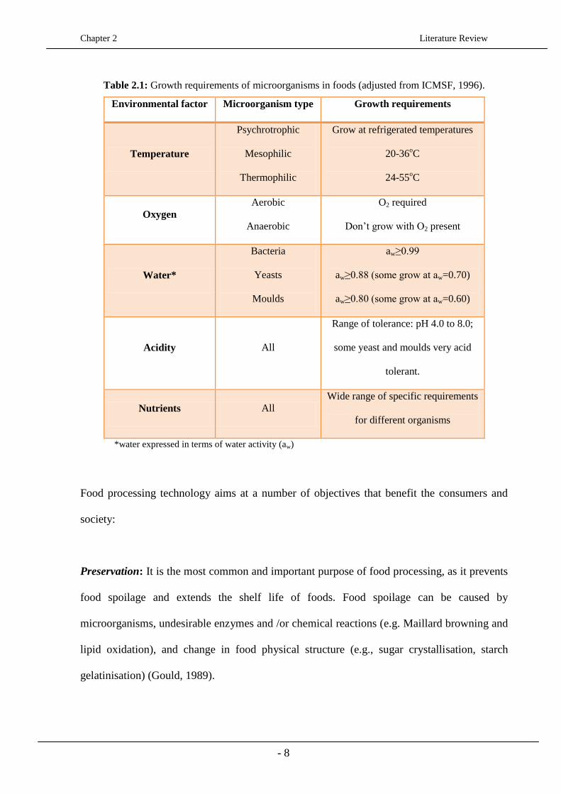
Table 2.1: Growth requirements of microorganisms in foods (adjusted from ICMSF, 1996). .............. 8
Table 2.2: Principal hurdles used for food preservation (Leistner, 1995; Lee, 2004). ......................... 18
Table 2.3: Pasteurisation processes for different foods (Adapted from Anon, 2007a; Campden BRI
technical manuals, 2006b). .................................................................................................................... 21
Table 2.4: z-values for heat-sensitive food components (Holdsworth, 1992). ..................................... 26
Table 2.5: Application of intrinsic and extrinsic TTIs ......................................................................... 46
Table 2.6: Applications of the various numerical models in the food industry .................................... 74
Chapter 3 - Pasteurisation of model food packages by the inversion method
Table 3.1: Model parameters of the fluids used. ................................................................................................. 128
Table 3.2: Thermal properties of fluids used. ..................................................................................................... 128
Table 3.3: Dimensionless numbers and velocity used in heat treatment. ........................................................... 130
Table 3.4: Equivalent processes of 5 min at 70oC at a calculated z-value of 10.8
oC. ......................................... 141
Chapter 4 - Modelling of temperature distributions in hot-filled food packages
Table 4.1: RMSE values (oC) obtained from the three cases of mesh resolution. .............................................. 160
Table 4.2: RMSE values (oC) for fluids A and T and Cases I and II. ................................................................. 178
Chapter 5 - TTI validation for hot-fill processes
Table 5.1: Bacillus amyloquefaciens α-amylase (BAA) characteristics (Tucker, 1999). ................... 187
Table 5.2: Application of BAA and BLA (Bacillus licheniformis) in food processing (CCFRA,
Pasteurization heat treatments, 1992). ................................................................................................. 188

List of Tables
- xiii
Table 5.3: Experimental immersion times and temperatures for BAA70 TTI. .................................. 194
Table 5.4: Experimental immersion times and temperatures for BAA85 TTI. .................................. 195
Table 5.5: Experiments conducted on Peltier stage at constant heating/cooling rate. ........................ 199
Table 5.6: Complex cycles produced on Peltier stage for a heating/cooling rate of .......................... 200
Table 5.7: Calculated DT-values for BAA70 and BAA85 solutions. ................................................. 201
Table 5.8: α-amylase TTIs used in pasteurisation treatments of foods .............................................. 203
Table 5.9: Properties of the fluids used at 70oC. ................................................................................ 214
Table 5.10: Possible scenarios for hot-fill processes. ......................................................................... 218
Table 5.11: Process values of thermocouples and BAA70 TTIs. ....................................................... 219
Table 5.12: ANOVA test for the correlation of BAA70 TTIs and thermocouples. ........................... 221
Table 5.13: Process values of thermocouples and BAA85 TTIs. ....................................................... 223
Table 5.14: ANOVA test for the correlation of BAA85 TTIs and thermocouples. ........................... 225
Nomenclature
- xiv
Nomenclature
Ao / Af Initial and final enzyme activity
aw Water activity
CBAA Concentration of BAA or BLA (mol l-1
)
Cp Heat capacity (J kg-1
K-1
)
C1 / C2 concentration of microorganisms at times t1 and t2
c and d Consistency and index constants
R Diameter of the container (m)
DT Decimal Reduction Time (min)
Do Decimal Reduction Time at a reference temperature To (min)
F Sterilisation value (min) and volume force (N m-3
)
Fo Target lethality at the coldest spot (min)
Fs Integrated lethality (min)
G´ / G´´ / G* Storage / loss / complex modulus (Pa)
Gr Grashof number (dimensionless)
g Acceleration of gravity (m s-2
)
hc Heat transfer coefficient (W m-2
K-1
)
H Height of the container (m)
i Complex number (√-1)
k Thermal conductivity (W m K-1
)
k’ Constant reaction rate
L Lethality (min) and length of container (m)
M Percentage of components on wet basis
N o / N f Initial and final number of microorganisms
N1 / N2 Number of spores at time t1 and t2
Nt Number of spores at time t
P Pasteurisation value (min)
p Initial pressure (Pa)
Pr Prandtl number (dimensionless)
q Inward heat flux (W m-2
)
Nomenclature
- xv
rA Reaction rate (mol s-1
)
Ra Rayleigh number (dimensionless)
Re Reynolds number (dimensionless)
t Duration of the heat treatment (min)
T(t) Product temperature (°C)
Tref Reference temperature (°C)
u Instantaneous velocity (m s-1
)
U Typical velocity (m s-1
)
x_wall / x_bot / x_lid Wall / bottom / lid thickness (m)
Xa,c,f,p,w Mass fraction of ash, carbohydrates, fat, protein, water
z z -value (number of degrees Celsius to bring about a ten-fold
change in Decimal reduction time) (°C)
Greek symbols
α Thermal diffusivity (m s-2
)
β Thermal expansion coefficient (K-1
)
Shear rate (s-1
)
minmax / Minimum and maximum shear rate (s-1
)
δ Phase angle (degrees)
δM / δT Momentum and thermal boundary layer thickness (m)
η0 and η∞ Viscosities at shear rate = 0 and = ∞ respectively
μ Dynamic viscosity (Pa s)
ν Kinematic viscosity (m2 s
-1) and velocity (m s
-1)
ρ Density (kg m-3
)
τmin / τmax Minimum and maximum shear stress (Pa)
σ Surface tension (N m-1
)
Nomenclature
- xvi
Abbreviations
2D Two dimensional
3D Three dimensional
12-D 12-log decimal reduction of microorganisms
ANOVA Analysis of Variance
BAA Bacillus amyloliquefaciens
BLA Bacillus licheniformis
CCRFA Campden and Chorleywood Food Research Association
CFD Computational Fluid Dynamics
CFL Courant Friedrichs Lewy condition
CMC Carboxymethyl Cellulose
df Degrees of freedom
DRT Decimal Reduction Time
EO Ethylene Oxide
FD Finite Difference
FE Finite Element
HACCP Hazard Analysis Critical Control Point
HCl Hydrochloric acid
HTST High Temperature Short Time
IR Infrared Radiation
LLP Least Lethality Point
LVR Linear Viscoelastic Region
MRI Magnetic resonance imaging
MS Mean Squared Error
NAS National Academy of Sciences
PEPT Positron Emission Particle Tracking
PPC Post Pasteurisation Contamination
RMSE Root Mean Square Error
SS Sum of Squares
TDT Thermal Death Time
TTI Time Temperature Integrators

Nomenclature
- xvii
Tris Tris hydroxymethyl aminomethane
UHT Ultra High Temperature
UV Ultra Violet
Chapter 1 Introduction
- 1
Chapter 1 - Introduction
Thermal processing has always been key in ensuring the microbiological safety of long-life
food and beverage products, whether that be a full sterilisation, aimed at a 12-Log reduction
of Clostridium botulinum, or a lesser pasteurisation heat treatment targeting less heat-resistant
organisms (e.g. Listeria monocytogenes, Escherichia coli O157, Salmonella) with other
inhibiting steps (pH control, water activity, etc.) (Holdsworth, 1997).
Manufacture of a thermally processed food consisted of two basic steps (Fellows, 2000):
Heat application to the food product to reduce microbial population to a level that is
acceptable; i.e. to achieve a statistically small probability of growth of pathogenic and
spoilage organisms under the intended storage conditions.
Sealing of the food product within a hermetic package to prevent re-infection.
In traditional preservation methods, such as canning, the food is sealed in its package before
heat is applied to it, whereas in aseptic treatments such as, hot-fill, cook-chill and cook-freeze
the food is heated before being dispensed into the pack (Rickman, 2007). The most heat-
resistant pathogen that survives thermal processing of low-acid foods is the spore-forming
organism Clostridium botulinum; a sterilisation process is established based on the 12-log
reduction of the Clostridium botulinum spores (i.e. 1 spore surviving in 1012
packs). However,
there is a growing trend to apply additional hurdles to microbial growth that allow the
processor to use milder heat treatments such as pasteurisation; the treatment is extensively
used in the production of many different types of food, such as fruit products, pickled
vegetables, jams and ready meals (CCFRA, 1992a). Food may be delivered in-pack

Chapter 1 Introduction
- 2
(analogous to canned foods), or in continuous processes (analogous to aseptic filling
operations). The target aimed during pasteurisation processes is usually a 5 or 6-log reduction
of the target organism. However, pasteurised foods are not free from microorganisms and rely
on other preservative mechanisms to ensure their extended stability for the desired length of
time (Montville,2005).
Of primary interest in the current work are foods that are given a mild heat treatment, more
specifically the hot-filled ones. Food products with a shelf-life of up to 10-days are
recommended to receive a pasteurisation treatment at least equivalent to 2 min at 70°C at the
product's thermal centre, i.e. the coldest point (CCFRA, 2006). This assumes that no other
preservation hurdle (e.g. salt, sugar or preservatives) is used, apart from chilled storage.
Examples of food products receiving this type of treatment are soups, sauces, cooked poultry,
ready meals and a wide range of pies and pastries.
With the number of products and their variety increasing, food companies are faced with the
challenge of proving that their products are safely pasteurised. Their ability to validate this
can be challenging if conventional temperature probe systems cannot be used. This might be
due to complexities introduced by products cooked in continuous ovens or fryers (e.g. poultry
joints, bread) or by particulate products cooked in agitated vessels or heat exchangers (e.g.
ready meals, soups, dressings) (Tucker et al., 2000). Thus, alternative validation approaches
are required.
The use of correct guidance and statistical models to validate and optimise processes can
result in several benefits, including significant cost reduction through use of less energy and
shorter process cycle times, which increases productivity and plant efficiency. It may also
lead to the improved retention of various nutrients in food products (Âvila and Silva, 1999).

Chapter 1 Introduction
- 3
1.1 Objectives
The objectives of the current study are:
To investigate the effectiveness of the inversion step in hot-fill processes as a thermal
treatment of the headspace and lid, for reducing post-pasteurisation treatments.
To test the reliability and accuracy of TTIs, when subjected to a variety of time-
temperature profiles, relevant to industrial thermal processes ;
To test the effectiveness of TTIs as a monitoring technique, for validating pasteurisation
processes.
To develop a valid mathematical model that would be able to accurately predict
temperature profiles and flow patterns of complex processes; simulating the inversion step
of the hot-fill treatment is one such a challenge.
1.2 Thesis chapters
This thesis has the following structure:
Chapter 2 reviews:
The food preservation methods used in the food industry, with thermal processing being
more extensively analysed;
The development of the TTI systems and their application up to date;
The development of a kinetic and heat transfer model used for designing, controlling and
optimising thermal processes

Chapter 1 Introduction
- 4
Chapter 3 refers to the experimental work carried out for investigating the effectiveness of the
inversion step as a treatment of the headspace and the lid, in hot-fill treatments. The method
aims at a target process of 5 min at 70oC for food products with a chilled shelf-life up to 10
days.
Chapter 4 illustrates the effectiveness of the finite element mathematical method in predicting
the flow behaviour of a starch solution and tomato soup during the cooling phase of the hot-
filling process. The model is validated by experimental data.
Chapter 5 investigates:
The sensitivity and accuracy of TTIs under isothermal and non-isothermal condition;
Their effectiveness as an alternative monitoring technique in monitoring pasteurisation
treatments, by being compared to temperature probes.
Chapter 6 summarises the conclusions of the current work and refers to future work
recommendations.
Publications: Papers and Posters are given in the CD included with this work at the back of
the thesis
Journal (Peer-Reviewed)
Peter J. Fryer, Mark J.H. Simmons, Phil W. Cox, K. Mehauden, Suwijak Hansriwijit, Flora
Challou, Serafim Bakalis, (2011). Temperature Integrators as tools to validate thermal processes
in food manufacturing. Procedia Food Science. 1, 2011, 1272 - 1277,
doi:10.1016/j.profoo.2011.09.188.
Chapter 1 Introduction
- 5
Conferences
Flora Challou, M. J. Simmons, P. J. Fryer (2014). Surface Pasteurisation of Food
Packages by the Inversion Method and evaluation of Time Temperature Integrators.
Institute of Food Technologists (IFT14), New Orleans, LA, USA, June 2014 (Poster
presentation)
Flora Challou, M. J. Simmons, P. J. Fryer (2015). Surface Pasteurisation of Food
Packages by the Inversion Method. International Congress of Engineering and Food
(ICEF12), Quebec City, Canada, June 2015, (Oral presentation).
Chapter 2 Literature Review
- 6
Chapter 2 - Literature Review
2.1 Introduction
Consumers’ demand for safe and high quality food products is ensured by the application of
different preservation techniques. Whilst the heat treatment of food products has been
extensively studied, no guidelines exist currently for the surface treatment of food packages
(CCFRA, 2012). Hot-fill treatment is based on the assumption that the heat transferred from
the pasteurised food is sufficient to decontaminate the package. That is true for the surfaces
that come in contact with the product, but it is not the case for the headspace and the lid of the
package. It is thus usual that foods are either over-processed before filling, or the product is
given a further heat treatment after filling. Usually, the after filling step is followed by a top-
up pasteurisation which includes either:
o Passing the food packages (jars or bottles) through a pasteurisation tunnel where water is
sprayed at high temperatures (around 95oC), or
o Inverting the package for pasteurising the headspace and the lid; the latter has been
extensively used in the food industry for filling into glass jars, plastic pots and pouches,
cartons and plastic trays.
Quantifying the heat treatment given to food packages during hot-fill operations would
potentially increase line efficiency and reduce waste and energy input (CCFRA, 2011).
In the current chapter, the state of work on heat treatment quantification by a variety of
validation techniques and optimisation methods is detailed.
Chapter 2 Literature Review
- 7
2.2 Food processing technology
Food processing is more than merely a necessity to preserve foods; multiple objectives are
served until the food product reaches the consumer. For instance, freezing technology both
preserves foods and offers convenience, while heating or fermentation of foods like soy
makes them edible and prevents them from mild toxicity caused by hemagglutinens (Floros,
2008). Food processing operations dealing with raw materials or ingredients that carry
pathogens are tightly controlled by regulations associated with detection and inactivation of
food-borne microorganisms in order to ensure that the final product delivered to the
consumers is safely delivered and of high quality. New, innovative technologies have been
developed to ensure not only the safety and quality of food products, but also to produce
foods with unique attributes (e.g. functional foods) (Cardello, 2002).
Most food preservation techniques are designed to create unfavourable conditions for
microbial growth. Some of the most important growth requirements of microorganisms,
associated with food preservation are presented in Table 2.1.
Chapter 2 Literature Review
- 8
Table 2.1: Growth requirements of microorganisms in foods (adjusted from ICMSF, 1996).
Environmental factor Microorganism type Growth requirements
Temperature
Psychrotrophic
Mesophilic
Thermophilic
Grow at refrigerated temperatures
20-36oC
24-55oC
Oxygen
Aerobic
Anaerobic
O2 required
Don’t grow with O2 present
Water*
Bacteria
Yeasts
Moulds
aw≥0.99
aw≥0.88 (some grow at aw=0.70)
aw≥0.80 (some grow at aw=0.60)
Acidity All
Range of tolerance: pH 4.0 to 8.0;
some yeast and moulds very acid
tolerant.
Nutrients All
Wide range of specific requirements
for different organisms
*water expressed in terms of water activity (aw)
Food processing technology aims at a number of objectives that benefit the consumers and
society:
Preservation: It is the most common and important purpose of food processing, as it prevents
food spoilage and extends the shelf life of foods. Food spoilage can be caused by
microorganisms, undesirable enzymes and /or chemical reactions (e.g. Maillard browning and
lipid oxidation), and change in food physical structure (e.g., sugar crystallisation, starch
gelatinisation) (Gould, 1989).

Chapter 2 Literature Review
- 9
Microbial food spoilage is the most important type of spoilage as it can cause quality and
safety deterioration that can range from merely a poor, non–nutritive product to food
poisoning (Miller, 1989).
Safety: The major concern and challenge of food processing operations is to inactivate
pathogenic microorganisms which are related to health hazards. The pathogens of concern
vary significantly in terms of heat resistance; Campylobacter, Salmonella, and Listeria are
heat-labile and can be inactivated by mild heat treatments such as pasteurisation, whilst
Bacillus cereus survives pasteurisation and low temperatures (Hammer, 1999).
Clostridium botulinum is the most heat-resistant bacteria which make it a good indicator for
the validation of thermal processes such as sterilisation and canning (Holdsworth, 1997).
Besides from the foodborne pathogens, other microorganisms such as yeasts, moulds, and
gas-producing bacteria can also cause food spoilage and thus must be inactivated (Sivertsvik
et al., 2004). The behaviour of microorganisms changes according to the environment they
are submitted to. Environmental factors such as the pH, water activity, chemical composition
and the properties of the foods themselves affect the microorganisms’ heat resistance and
behaviour. Thus, the type of microbial flora associated with raw materials or ingredients is
important to be known, before any thermal process is applied. Another important factor to be
taken into consideration is the re-infection of the product, which can cause problems in the
thermal treatment (Lioliou et al., 2004). Safety is also associated with other factors such as
pesticides, natural toxins, antibiotics and environmental contaminants (NAS, 1973).
Managing microbiological risks is not the only task that ensures the safety of a final product:
good agricultural and manufacturing practices that address chemical and physical hazards are
also of great importance (Hall, 1977).

Chapter 2 Literature Review
- 10
Quality: It refers to attributes such as colour, taste, texture, nutrient content (e.g. vitamins)
and aroma. The quality of most attributes starts declining at the moment the foods or
ingredients are harvested or collected (Kader, 2005). Thus, processing operations need to
ensure that the rate of decline of the quality attributes is slowed down and the losses are
minimised. A good example is the blanching of vegetables after they have been harvested; the
nutrients are almost kept at their initial level (Barrett, 2007). The challenge that food
manufacturers have to face is to ensure safety, without compromising quality. Therefore, it is
important to understand the reaction kinetics in relation to microbial inactivation, chemical
damage, enzyme inactivation and physical changes.
Availability and sustainability: The increased demand for access to a variety of food products
all year along requires food processes to be fast and efficient. Controlled atmosphere for
stored fruits and vegetables is an example of retaining freshness and extending shelf-life
(Rickman, 2007b). The goal of sustainability is to maximise the utilisation of the raw
materials required for manufacturing purposes, and the integration of the activities from the
production to the consumption stages (Bongiovanni, 2004). To maximise the conversion of
raw materials into final products, postharvest losses need to be reduced and the utilisation of
by-products need to be increased. Then, efforts need to be made for ensuring that resources
such as energy and water are efficiently used, with minimal environmental impact.
Refrigeration of fresh food products is an example of minimising loss and increasing the
edible life of the product (Mattsson, 2003).
Chapter 2 Literature Review
- 11
Convenience, Health and Wellness: Food processing is also used for preparing ready-to-eat
foods and meals that need a limited amount of effort to be cooked before consumption. For
instance, many frozen or refrigerated products only need to be microwave-heated for only a
few minutes. Snacks are another example of convenience products achieved by food
processing. Besides meeting nutritional requirements, food can also be processed in ways that
provide them with optimised properties, promoting health and wellness. Refining of anti-
nutritional compounds in vegetables, extraction of carotenoids from tomatoes, for improving
bioavailability and nutritional quality, are some of the techniques used to optimise quality of
foods (ILSI, 2004a). Some products are designed and produced to respond to specific
nutritional needs of the consumers, such as gluten free products, sugar free, reduced salt, etc.
Other products are enriched with vitamins, minerals or other nutrients (e.g. addition of
calcium in orange juice, stanols in margarine) for bone and heart health respectively. These
products are called functional foods and are required to also meet the consumers’ expectations
of flavour and texture (Rosetta Newsome, 2007).
With preservation being the most important objective of food processing, the following
technologies are used to control the different spoilage types in food products:
Thermal processing: Thermal processes can range from mild, such as blanching and
pasteurisation, to severe, such as sterilisation and canning (Leistner, 1995). Depending on the
resistance of the attribute targeted, a variety of time-temperature combinations is applied. In
the case of mild processes, vegetative pathogens, yeasts, moulds and/or enzymes are targeted
and need to be inactivated. When the spore-forming and toxic pathogens are targeted, more
severe conditions need to be applied and destroy the microorganisms implicated. The high
temperature exposure of foods ensures safety, but at the same time causes quality alterations.

Chapter 2 Literature Review
- 12
When the quality attributes (e.g. nutritional value, texture, flavour, etc.), are changed in an
undesirable way, the thermal process is referred to as “thermal damage”, but when desirable,
the process is known as “cooking”. The preservation by heat will be further discussed in §
2.2.1.
Low-temperature processing: When compared to heating processes, the activity of the
microorganisms and enzymes, under low temperatures, is not destroyed or inactivated but
depressed, for as long as the applied temperature conditions (chilling or freezing) are kept
constant. Unlike heat preservation, low temperature preservation is reversible, and once
temperature is increased, microorganisms and enzymes will be reactivated. Hence, it is critical
to maintain the required low temperatures throughout the product’s shelf life. Low
temperature preservation can be divided into two processes; chilling, where the food is kept at
a low temperature above its freezing point, and freezing, where the food is kept at a
temperature below its freezing point (Fellows, 2000). Besides from temperature differences,
the processes differ also in terms of phase change that happens during freezing, due to
reduced molecular mobility. The water transition to ice in freezing results in water activity
reduction in the rest of the food that is not ice and consequently microbial and enzymic
depression. The phase transitions during freezing can also lead to undesirable and irreversible
changes, such as texture alteration (Heldman and Hartel, 1997; Boonsupthip, 2007).
Dehydration: The process is one of the oldest and most energy intensive food preservation
techniques used (Von Loesecke, 1943; Saravacos, 1965; King, 1968; Thijssen, 1979). It aims
at slowing the growth of microorganisms and rate of chemical reactions. The method offers
many advantages to food processors, since volume and weight of the product are reduced by

Chapter 2 Literature Review
- 13
water removal, the shelf life is extended, and liquids are converted into powders, such as
instant coffee. Water is usually evaporated, vaporised, or sublimated in the case of freeze-
drying by means of a simultaneous heat, mass, and momentum transfer mechanism (Whitaker,
1977) within the food and between the food and the drying medium. In addition to water
removal, other reactions that modify the original structure of the food material also occur
(Viollaz and Alzamora, 2005); chemical reactions such as Maillard browning of amino
acids/reducing sugars, sugar caramelisation, protein denaturation, and pyrolysis of organic
constituents, as well as loss of volatile compounds and gelatinisation of starches, are some of
them.
Water activity (aw) preservation: Many processes and products have been successfully
designed based upon the aw concept (Alzamora et al., 2003). Unlike water content, aw can
give information about the shelf stability of the food. The free water available in fruit and
vegetables supports microbial growth, chemical reactions and acts as a transporting medium
for compounds, whilst the bound water does not participate in these reactions since it is bound
by water soluble compounds such as salt, sugar, gums, etc. and by the surface effect of the
substrate matrix binding (Barbosa-Canovas et al., 2007). The moisture conditions in which
spoilage microorganisms cannot grow is very important for food preservation; each
microorganism has a critical aw below which it cannot grow. At aw=0.3, food products are
very stable in terms of enzyme activity, non-enzymatic browning, lipid oxidation and
microbial parameters. As aw increases, the probability of the food product deteriorating
increases (Barbosa-Canovas et al., 2007).
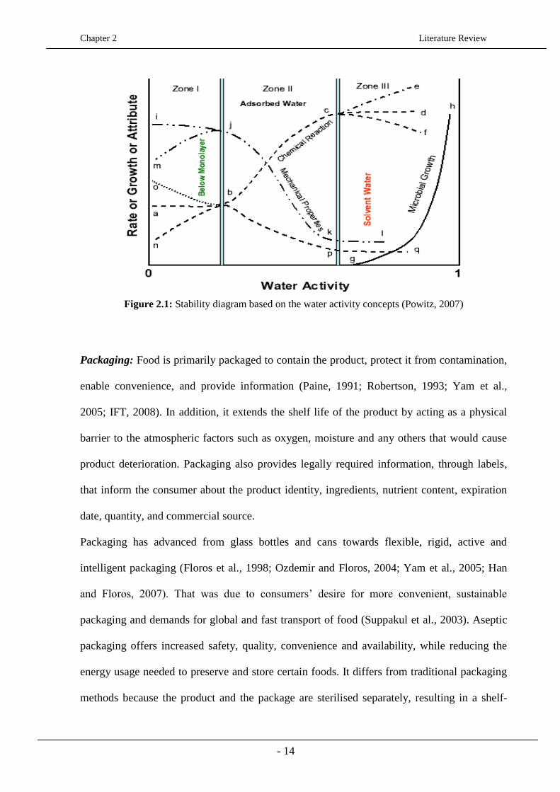
Chapter 2 Literature Review
- 14
Figure 2.1: Stability diagram based on the water activity concepts (Powitz, 2007)
Packaging: Food is primarily packaged to contain the product, protect it from contamination,
enable convenience, and provide information (Paine, 1991; Robertson, 1993; Yam et al.,
2005; IFT, 2008). In addition, it extends the shelf life of the product by acting as a physical
barrier to the atmospheric factors such as oxygen, moisture and any others that would cause
product deterioration. Packaging also provides legally required information, through labels,
that inform the consumer about the product identity, ingredients, nutrient content, expiration
date, quantity, and commercial source.
Packaging has advanced from glass bottles and cans towards flexible, rigid, active and
intelligent packaging (Floros et al., 1998; Ozdemir and Floros, 2004; Yam et al., 2005; Han
and Floros, 2007). That was due to consumers’ desire for more convenient, sustainable
packaging and demands for global and fast transport of food (Suppakul et al., 2003). Aseptic
packaging offers increased safety, quality, convenience and availability, while reducing the
energy usage needed to preserve and store certain foods. It differs from traditional packaging
methods because the product and the package are sterilised separately, resulting in a shelf-
Chapter 2 Literature Review
- 15
stable final product with high quality and extended shelf life; that is mainly due to the milder
heat treatment that the product undergoes compared to the traditional thermal process (Floros,
1993).
Chemical preservation: This type of preservation is based on the addition of chemicals in
foods, known as food preservatives; salting is one of the oldest and most common chemical
preservation techniques. Smoking can also be used as a chemical preservation method due to
the deposition of naturally produced chemicals resulting from thermal breakdown of wood
and salting; the incorporation of smoke flavour and the development of colour are highly
desirable in the developed societies (McGee, Harold, 2004).
Most of the food pathogens cannot grow or survive at low pH conditions; compounds that
lower the pH of the food product or its surrounding environment need to be used. Such
compounds can be acids (e.g. citric acid, vinegar, acetic acid, lactic acid produced by
fermentation), herbs and spices, or non-natural chemicals (e.g. sorbic acid, sulphur dioxide)
(Jay, 1995).
Novel, alternative processes: The new processing technologies include microwave, ionizing
radiation, pulsed electric fields, ultra-high pressure, high-intensity pulsed light and ohmic
heating (Raso, 2003). These are claimed to deliver safe and shelf-stable food products much
faster than canning or other conventional thermal processes, but have not yet been widely
used in the industry. The novel processes, primarily developed to replace the conventional
thermal processes and have the potential to be used in a variety of food products that will
meet consumers’ growing demands for fresh-like and nutritious foods. Each of the emerging
Chapter 2 Literature Review
- 16
technologies has unique characteristics and potential applications in a variety of food
products.
o Microwave Heating: A well-known and widely accepted technology by the consumers
for heating prepared foods and cooking raw ones.
o Ohmic Heating: The process passes electricity through the food via contact with
charged electrodes, resulting in rapid and more uniform heating of the product. Heat is
generated instantly inside the food, and its amount is directly related to the voltage gradient,
and the electrical conductivity (Sastry and Li, 1996). The lack of high wall temperatures, the
short processing time and the maintained quality factors such as colour and nutritional value
are some of the an advantages of ohmic treatments over conventional methods (Wang and
Sastry, 2002; Castro et al., 2004a; Icier and Ilicali, 2005a; Leizerson and Shimoni, 2005a, b;
Vikram et al., 2005). Ohmic treatment is used in a wide range of applications such as
blanching, pasteurisation and sterilisation (Lima and Sastry, 1999), and mostly for heat-
sensitive foods (Ramaswamy et al., 2005), such as fruit and liquid eggs.
o High-Pressure Processing: a cold pasteurisation method according to which food
products are sealed, placed into a containing liquid chamber, and pumps are used to create
high hydrostatic pressures (HHP) of up to 600 MPa for a few seconds to a few minutes. The
technique is a promising preservation method that respects the quality attributes of food, since
the reduction in microbial populations can be accomplished without significant increase in
product temperature. HPP is especially efficient on food products, such as yogurts and fruits
(Brown, 2007) as pressure-tolerant spores do not survive at low pH levels (Adams & Moss,
Chapter 2 Literature Review
- 17
2007). A number of ready-to-eat meats and other refrigerated items have been treated by high
pressure, resulting in high-quality products with increased shelf life (Jay et al., 2005).
o Pulsed Electric Fields (PEF): The method uses high voltage (>20 kV) and short (μs)
electric pulses to liquid or semi-solid food products placed between two electrodes. It aims for
microbial inactivation, whilst causing minimal effect on food quality attributes (Quass, 1997),
making the technology highly advantageous as compared to traditional thermal processing.
Most of the PEF studies are concerned with the microbial inactivation in liquid foods (Qin et
al., 1995). However, recent research has shown that PEF is very effective for inactivation of
microorganisms, increasing the pressing efficiency and enhancing the juice extraction from
food plants, and for intensification of the food dehydration and drying (Barsotti and Cheftel,
1998, 1999; Estiaghi and Knorr, 1999; Vorobiev et aI., 2000, 2004; Bajgai and Hashinaga,
2001; Bazhal et aI., 2001; Taiwo et aI., 2002).
Hurdle technology: It is based on the principle that the combined effect of different
preservation techniques is more efficient than using each technique separately (Leistner,
2002). For instance, the process of dried sausages includes steps that need to ensure low pH,
low water activity, low temperatures, salting, smoking, and the addition of herbs or spices.
The required, preserved final product is achieved by the combination of all the steps, as each
one individually would not be sufficient.

Chapter 2 Literature Review
- 18
Table 2.2: Principal hurdles used for food preservation (Leistner, 1995; Lee, 2004).
Parameter Symbol Application
High temperature F Heating
Low temperature T Chilling, freezing
Reduced water activity aw Drying, curing, conserving
Increased acidity pH Acid addition or formation
Reduced redox potential Eh Removal of oxygen or addition of ascorbate
Bio-preservatives
Competitive flora such as microbial fermentation
Other preservatives
Sorbates, sulfites, nitrites
2.2.1 Thermal processing of food products
The application of high temperatures on food products, their surrounding environment and
package, is the basis of heat preservation, which is the most common type of preservation
method. It is the principle preservation method used in the canning industry. Thermal
processes can be mild, as in the case of blanching and pasteurisation or more severe as in
canning operations, all relying on the application of heat. Depending on the intensity of the
thermal process food safety and quality are affected accordingly. The reasons why foods are
heated are numerous, with preservation being the primary one, as it is associated with the
microbiological safety of a product, which can be at risk if certain heat-resistant food
pathogens are not destroyed or inactivated (CODEX, 1997).
The effectiveness of a thermal process is dependent on the formulation and composition of the
food product, the heat resistance of the microorganisms present in each of the products, the
heating rate of the specific product and the container’s characteristics. The product’s physical
thermal properties, especially its rheology (if a liquid), have a significant effect on the heat

Chapter 2 Literature Review
- 19
transfer mode and the heat penetration speed (Lewis, 2002). In a pure solid and liquid food,
heat will be transferred by conduction and convection, respectively, but for most viscous
fluids or solid-liquid mixtures the heat transfer mechanisms will lie between the above two
extremes. According to HACCP procedures, it is important to find the coldest spot, i.e. the
point in the pack or vessel that heats slowest.
Thermal transfer to this point is the slowest and thus controls the process. That can be an easy
task when it comes to solid products, where the cold spot is located in the centre of the
container, but not as easy when complex food products such as viscous fluids or particulate
mixtures are involved; for locating their slowest heating point, the determination of heat
penetration data is of great importance. Another reason for heat to be applied in foods is
associated with quality issues. Chemical reactions like protein denaturation and starch
gelatinisation are promoted, and the quality attributes of the final product are affected either
advantageously or not. For instance, the gelation of evaporated milk is prevented by heat
application, and the texture of yoghurt is improved, while in other products foods where a
natural and fresh appearance is required such as in drinkable milk or fruit juices the sensory
and nutritional quality is damaged by heat. Enzyme activity may also result in quality
changes; some enzymes need to be inactivated for avoiding changes like fruit browning by
polyphenol oxidases and minimising quality changes such as flavour, caused by lipases,
whilst other enzyme action can improve the taste and structure of products like bread,
biscuits, wine and beer (Campbell et al., 1999).
Safety and quality issues can conflict in cases where severe heat treatments are applied;
microbial inactivation is achieved, but at the same time the quality of the product deteriorates.
Most biochemical reactions involved in quality degradation are catalysed by heat-sensitive
enzymes (Meade et al., 2005). Hence, the quality deterioration can be prevented and the food
Chapter 2 Literature Review
- 20
quality can be retained. Similarly, a food product is microbiologically stable, when the heat
applied is sufficiently high and it is hermetically sealed. Therefore, to extend the shelf-life of
a food product, the denaturation of enzymes, destruction of bacterial spores, and the
inactivation of vegetative pathogens, need to be achieved. To achieve all three objectives
would result in a stable product with a much extended shelf-life. Generally, the thermal
processes aiming at each of the above objectives, besides cooking, are blanching,
pasteurisation and sterilisation, with the latter two being tightly controlled and regulated by
government and state agencies, due to their impact on health and wellness (Singh et al., 2004).
Blanching
Blanching is a mild, pre-heating step that is applied to food products at temperatures <100oC
for a couple of minutes and it is usually followed by other heat treatments, such as freezing
and drying (Van Buggenhout 2005). Due to being mild, the process has limited effect on
nutrients. Blanching may simply be a cooking process wherein foods, normally vegetables
and some fruits are immersed in boiling water or are steamed for a very short time (seconds to
a couple of minutes) and are then immediately cooled down into cold/ice, for the cooking
treatment to be halted, which can lead to quality deterioration of the products. The cooking of
asparagus and protein-based salads are characteristic examples of blanching. They are boiled
for 30 seconds and then chilled rapidly. Blanching is also used to inactivate anti-nutritional
properties (e.g. trypsin inhibitor found in soybeans), and reduce oxidation by removing air in
the food tissues (Selman., 1987).

Chapter 2 Literature Review
- 21
Pasteurisation
Pasteurisation is also a relatively mild heating regime, in which food is heated to < 100ºC, and
it aims to inactivate heat labile microorganisms, such as vegetative bacteria, yeasts, moulds,
and/or enzymes that may cause food spoilage. It is applied to a wide, diverse range of foods
such as dairy products, fruit, vegetables, drinks, meat, fish, sauces, etc. in order to extend their
shelf-life from a few days up to several months, depending on their acidity. The heat
treatment is in most cases combined with rapid cooling and refrigeration, in order to avoid
post-pasteurisation contamination (PPC) from occurring. Some examples of food products
and the reasons they are pasteurised, are presented in Table 2.3.
Table 2.3: Pasteurisation processes for different foods (Adapted from Anon, 2007a; Campden BRI
technical manuals, 2006b).
Food
product Purpose Factors
Target
organism
Processing
conditions
Acidified
vegetables
Ambient shelf
stable pH must be < 4.0
Butyric
anaerobes
15 min at 100oC
(retort)
Equivalent process:
5 min at 85oC
Beer Ambient shelf
stable
CO2 acts as
inhibitor Yeasts 20 min at 60
oC
Brown
sauce
Ambient shelf
stable
pH=3.6±0.3
acetic acid, salt,
sugar, spices
Yeasts, moulds,
lactic acid
bacteria
30 s at 90oC (plate
heat exchanger)
Canned
plums
Ambient shelf
stable
pH=3.5
sugar 30oBrix
Enzyme
inactivation,
yeasts
125 min at 101oC
(retort)
Equivalent process: 5
min at 85oC
Canned
tomato
sauce
Ambient shelf
stable
pH=4.2
citric acid, salt,
sugar
Butyric
anaerobes
70 min at 105oC
(continuous
steriliser)

Chapter 2 Literature Review
- 22
Food
product Purpose Factors
Target
organism
Processing
conditions
Carrots
and onions
in wine
sauce
Ambient shelf
stable pH must be < 4.0
Enzyme
inactivation
10 min at 110oC
(retort)
Equivalent process: 5
min at 85oC
Milk
Pathogen
destruction and
extended chilled
shelf-life at
T≤3oC
Chill storage
Pathogens
(Mycobacterium
tuberculosis)
15 s at 72oC (heat
exchanger)
Fish pate
Short shelf life-
chilled stability
at T≤3oC
aw=0.97 Listeria
4 h at 82oC (oven)
Equivalent process:
12 min at 70oC
Meat
Chilled stability
at T≤3oC
(6 weeks shelf
life)
Salt 2.5% Psychrotrophic
C.botulinum
7.75 h at 78oC (oven)
Equivalent process:
10 min at 90oC
Soft drinks Ambient shelf
stable pH=3.2-3.5 Yeasts
4-10 s at 90-95oC
(heat exchanger)
Tomato
ketchup
Unopened
ambient shelf
life
pH=3.8-3.9
acidity 1.5%
sugar 26%
salt 2.9%
Z.bailii
2.3 min at 82oC (min.
in bottle)
Equivalent process: 3
min at 82oC
Pasteurisation can be delivered 'in-pack' or to products that are thermally processed before
being filled. In-pack pasteurisation is a very conventional concept, as the food product is
sealed in a container and then thermal process is applied to both the food product and the
container. The thermal process may be batch, with the retort being used for the heating,
holding and cooling phases of the treatment, or continuous, where the food products roll on
conveyors into a tunnel with the three sections of heating, holding, and cooling (Fellows,
1997). In a hot-fill process, the food is pasteurised before being filled into the package,

Chapter 2 Literature Review
- 23
assuming that the temperature given to the food will sufficiently pasteurise the package.
However, no guidance exists on this subject (CCFRA, 2007) and the uncertainty has led the
hot-filled products to often be processed to higher temperatures than necessary before filling,
or the product to be given a further heat treatment after filling and sealing the package (Figure
2.2). It is often the case that the food product temperature drops dramatically as it comes into
contact with the food pack and, consequently, provides little thermal decontamination on the
inside pack surface. Experimental results obtained from industrial trials showed that there was
a significant temperature decrease in certain containers after the hot-fill treatment (CCFRA,
2014); a temperature reduction of up to 20˚C was observed on glass jar packages, 5-10˚C for
plastic surfaces and up to 3˚C for pouch surfaces, as compared to the temperature recorded at
the bulk of the food product. This suggests that hot-filling alone is not realistic for achieving
even a minimum of 70°C for 2 minutes process, if the packages is not pre-heated or/and post-
pasteurised.
Figure 2.2: Typical post-filling pasteurisation tunnel

Chapter 2 Literature Review
- 24
In hot-filling processes, products are thoroughly cooked before being filled into the package.
Thus, any spoilage occurring in the final products, would probably be due to either
insufficient heating of the internal surfaces of the package, or because of post-process
contamination caused by failure of the package (Bown, 2003).
Both in-pack and hot-fill methods are time-consuming and expensive, and often require
significant additional processing capability. The quantification of hot-fill operations would
potentially be advantageous in saving water and energy, reduce waste and have great
environmental impact.
Research concerning the application of hot-fill treatment in products like fruits, fruit purees,
tomato sauces and pastes, has been covered in literature. A standard procedure for the hot-fill
treatment of fruits with a pH < 4.0, was recommended by the National Canners Association
(Brown, 1984) and includes the following conditions: filling temperature >85°C, can sealing,
water processing for 2 minutes at 88°C, steam can also be used, and cooling. The above
conditions appeared to be ineffective, however, when applied in Indian canneries, due to the
long holding time (10-30 min) between sealing and processing (Silva, 1997). Nanjundaswamy
et al., (1973) evaluated the impact of the hot-fill process in canned mango products, and
concluded that yeast and peroxidase inactivation, as well as the reduction of the overall
process time, are significantly affected by the filling temperature. Cans of a 570 mL capacity,
were hot-filled at temperatures from 76 to 80°C, sealed, inverted for 2-3 minutes and cooled
down. The conditions used proved sufficient for the product to be pasteurised. The validation
of the process was based on the analysis of the final enzymic and microbiological activity.
Nath & Ranganna, (1983a) studied the impact of the hot-fill treatment on guava pulp, and
managed to determine heat transfer characteristics and process requirements.
Chapter 2 Literature Review
- 25
Sterilisation
Sterilisation is the heat treatment primarily used to inactivate microorganisms that cause food-
borne disease such as botulism, and other microorganisms related to food spoilage, such as
yeasts and moulds. Sterilisation can be delivered in two ways (Nelson, 2010):
o The food is sealed in a container and then it is thermally processed, together with the
package, referred to as canning or in-container processing.
o The food is sterilised, it is filled into pre-sterilised containers, within a sterile
environment and it is finally sealed. The method is referred to as aseptic processing. Whatever
the process, the safety and quality of the food need to be ensured. With Clostridium botulinum
being the critical target microorganism in sterilisation processes, low-acid food products with
a pH>4.5 would be the ones of interest. For a 12D reduction of C. botulinum, that would
ensure the required safety, the low-acid foods need to be processed for 3 min at 121oC, also
referred as a 3Fo process. The process value of the sterilised products is determined by
measuring the time-temperature history of the product at the slowest heating point, using a z-
value of 10oC, for C. botulinum. The ideal sterilisation process would involve the heat to be
instantaneously transferred to the food, so that the same temperature is reached by all food
parts, at the same time. In that case sterilisation reactions would predominate over the quality
ones (Fryer, 1997).
Ultra High Temperature (UHT) and High Temperature Short Time (HTST) processes are
considered to follow the above ideal concepts. In both processes food is rapidly heated at
about 130-140oC, is held for a few seconds at high temperatures, and then cooled down in the
same rate, in order to avoid product degradation. Both processes result in products with
substantially improved quality attributes compared to conventional heat treatments (Simpson
et al., 2000). More specifically, in the HTST process the food product is sterilised before it is

Chapter 2 Literature Review
- 26
filled into the package, which is also pre-sterilised using either steam or hydrogen peroxide.
The heat rates of HTST process are significantly higher than in canning, making the process
ideal for continuous operations.
The rate at which microorganisms are destroyed is increased with temperature. The same
thing happens with the rate at which a quality factor changes. However, the microbial
destruction rate is from four to seven times more temperature sensitive than the quality
degradation rate (Martinez et al., 1999; Holdsworth, 2004). Therefore, for every 10oC increase
in processing temperature, the cooking effect will be doubled, whereas the microbial death
rate will increase by a factor of ten (Table 2.4).
Table 2.4: z-values for heat-sensitive food components (Holdsworth, 1992).
Component z-value (oC)
Bacterial spores
7-12
Microbial cells
4-8
Enzymes
3-50
Vitamins
25-30
Proteins
15-37
Sensory factors
Overall
Texture-softening
Colour
25-47
25-47
24-50

Chapter 2 Literature Review
- 27
Thus, processing at high temperatures, and shortened processing time, the product delivered
would potentially be safe with a reduced quality loss. The question is how fast can the product
be heated and cooled. The UHT process has been used mostly for dairy products, especially
milk, when the conventional sterilisation processes cause sensory problems. UHT heat
processing results in ambient stable and better quality food products, as compared to
conventional sterilisation process. A comparison between conventional and aseptic processes
used in food industries, is illustrated in Figure 2.3.
Figure 2.3: Comparison of A. conventional and B. aseptic processing for the production of shelf
stable foods (Nelson, 2010).

Chapter 2 Literature Review
- 28
2.2.2 Surface decontamination of food packages
Most of the food contamination studies carried out in factories and labs refer to the
microorganisms present in the food. Hence, little information on package contamination, and
guidelines on the controls that need to be implemented for ensuring the required food safety
and quality, is available. The first step in understanding the degree of decontamination needed
to be achieved on the food package, is knowledge of the type and load of the microorganisms,
or enzymes present. Then, the extent of the heat treatment applied to the surface of the
package needs to be determined (CCFRA, 2012).
Aseptic packages utilise plastics, foil containers or paperboard for packing the sterilized
product. In hot-fill treatments, glass jars, laminated cardboard and plastic tubs are of
particular interest. Experiments conducted on concentrated tomato paste, hot-filled in glass
jars, showed that spoilage microorganisms such as Bacillus coagulans were not inactivated
after the application of the hot-fill treatment (Sandoval et al., 1994). Hersom and Hulland,
(1964) supported the above findings by spotting remaining Clostridium spores after hot-
filling. Vegetative pathogens, yeasts and moulds were observed by Tucker et al., (2004), on
the packaging used for dairy products, before they were hot-filled. The highest contamination
level appeared to be found on polystyrene surfaces, as compared to materials such as glass.
That is assumed to be because of the higher electrostatic charge observed on polystyrene, and
in plastic packages in general, making them a significant source of contamination.
The most common packaging heat treatments used include thermal processing (including
saturated and superheated steam), radiation, chemical methods and a combination of the
above (Ansari and Datta, 2003). Some of the methods used for sterilising aseptic packages are
summarised in the following paragraphs:
Chapter 2 Literature Review
- 29
Thermal process methods
As mentioned above, heat processing is still the most commonly used method for food
preservation and package decontamination. When heat is used, the nature of the material of
package needs to be taken into account. The low thermal conductivity of plastics and cartons
makes it more difficult to sterilise them as compared to metal packages.
Thermal processes do not cause environmental hazards, since they don’t deposit any
undesirable residues on the surface being treated.
Saturated steam and hot air (moist heat): It is mainly used for the sterilisation of
thermostable plastic cups and metal surfaces, such as homogenisers and fillers in the hold
tube. The moulded cups and foil lids are subjected to saturated steam at 165oC and 6 bar after
deep drawing. At the same time, the external cup surface is cooled by applying air to limit the
effect of the short time heat application on the material, by reducing the pressure, as the
materials cannot otherwise withstand the high temperatures for long (Larousse and Brown,
1997).
Superheated steam and hot air (dry heat): The heat delivered is not as effective as the
one obtained from moist heat at the same temperature for sterilisation, therefore higher
temperatures are required (Larousse and Brown, 1997).
The hot-air method is preferred over the saturated heat, when paper-based packaging is
involved, due to condensation and for food products with a pH of <4.6. The method can
ensure safety without any effect on packaging material quality (Toledo, 1986). Hot air
sterilisation has been commercially used for juice and beverages.

Chapter 2 Literature Review
- 30
o Heating by extrusion: It is a form, fill, seal packaging system that relies on the
temperatures reached by thermoplastic resin, during the co-extrusion process. The high
extrusion temperatures result in a sterile product contact surface. During the process, a multi-
layer package material is fed into the machine and is delaminated under sterile conditions. A
layer of material is then removed, and the product contact surface is exposed; the container
material is then thermoformed into cups (Bauser, 2006). The method has only been used for
acidic products with pH less than 4.6, due to concerns about its efficacy (Reuter, 1988).
Chemical methods
A variety of chemicals, either in a liquid or gas form are used as an alternative method for
surface decontamination of packages. The most commonly used ones are the following:
o Hydrogen Peroxide: It is the most widely used chemical disinfectant for packaging
materials, and it is efficient either at ambient temperatures and high concentrations, or at
increased ambient temperatures and lower concentrations. That is due to the slow reaction rate
of the chemical on the surface of the package, at ambient temperature. Swartling and
Lindgren (1968) note that spores of Bacillus subtilis were reduced by a 4-log, when the food
package was immersed for 15 seconds in a bath consisted of 20% of hydrogen peroxide, at
80oC. Rutherford et al., (2000) reported that the mechanisms of inactivation are different
between spores and vegetative cells. Hydrogen peroxide can be commercially applied to
packages by dipping (a bath consisted of 30-33% of hydrogen peroxide, where the package is
immersed), spraying (dispersed droplets of hydrogen peroxide are sprayed on the package
surface), and rinsing (substitutes the other two, when not feasible). Recent studies have been
Chapter 2 Literature Review
- 31
referring to hydrogen peroxide vapour (HPV), which is beneficial in disinfecting hard to reach
and complex surfaces (Johnston et al., 2005).
o Ethylene Oxide (EO): It is used mainly used as a chemical intermediate in the
manufacture of detergents, solvents, and textiles, but it has also been used in sterilising
packages for aseptically processed foods, dried fruits and spices (ATSDR, 1990). EO has
been successfully used for spice sterilisation with alkylation as a mechanism of action. Usage
of EO as a food sanitation method accelerated dramatically in the 1960s, when EO fumigation
was reported to significantly reduce spoilage organisms in spices and spice blends
(Radomyski, 1994). It is temperature, humidity and concentration dependent and is generally
carried out at temperatures of 30 °C to 60 °C with relative humidity above 30%, for sterilising
objects sensitive to temperatures greater than 60°C. The EO has been shown to be effective
when diffused freely throughout the product being treated, which means that the package used
needs to be breathable (Council of Agricultural Science and Technology, 1995).
Radiation methods
When thermal and chemical methods are not feasible, radiation methods are used as an
alternative approach which is becoming increasingly popular; Figure 2.4 illustrates the
mechanism of radiation, when applied to a surface. The packaging materials commonly used
in radiation are: PVC, polyethylene (PET), polypropylene, polyester, nylon, etc. (Ansari and
Datta, 2003). Radiation methods are classified as follows:
o Ultraviolet (UV) Ray: Both vegetative pathogens and heat-resistant spore-forming
bacteria are UV sensitive and are effectively destroyed at the range of 200-315 nm
Chapter 2 Literature Review
- 32
(Bachmann, 1975). UV light has been used in the food industry for disinfecting surfaces of
equipment in bakeries, cheese and meat plants, food packages such as bottles, boxes, foils,
caps, cartons and films and for decontamination of conveyor surfaces (C.A.C., 1994). UV
light has been effectively used to disinfect smooth surfaces, but its application in food
processing industry is still limited. Reasons for that can be the restricted range of
commercially available equipment for disinfecting solids and the fact that the kinetic data for
microbial inactivation are mostly obtained from in suspension in aqueous media or air
(F.D.A., 1997). A few studies have been reported on the use of UV irradiation for the
inactivation of Salmonella typhimurium on poultry carcasses (Wallner-Pendelton et al., 1994),
Escherichia coli and Salmonella on pork skin and muscle (Wong et al.1998); and Listeria
monocytogenes on chicken meat (Kim et al., 2002). The above studies showed that UV light
has the potential to decontaminate food surfaces from bacterial contamination and therefore
could possibly be used as post lethality treatment to control L. monocytogenes and other
pathogens of concern. A commercially available food surface decontamination system, called
the UV tumbling process was developed by C&S Equipment Company The system has been
recommended for the treatment of fresh fruits and vegetables, meats, frozen foods (fruits,
vegetables, meats, seafood, bakery products), and cooked, refrigerated products (pasta,
cheese) (Chapman, 2003).
o Infrared Radiation (IR): It is commonly used for decontaminating the interior of lids,
coated with aluminium and its working principle is based on the conversion of the radiation
into sensible heat, when it is in contact with an absorbent surface (Ansari and Datta, 2003).

Chapter 2 Literature Review
- 33
Figure 2.4: Extinction of radiation (Pan et al., 2010)
Application of IR in food processing has gained popularity due to its advantages over
conventional heating. It has been applied in a variety of processes such as drying, baking,
roasting, blanching, pasteurisation, and sterilisation of food products, showing a potential to
produce high-quality foods at low-cost (Sakai and Hanzawa, 1994). When used for
dehydrating foods, IR radiation is very advantageous since the drying time is reduced, the
energy efficiency is increased and there is uniform temperature throughout the product while
drying. Thus, the necessity air flow across the product is reduced and better-quality finished
products are obtained (Dostie et al., 1989; Navari et al., 1992; Mongpreneet et al., 2002).
Because of the its advantageous effect in the drying process, IR has been successfully applied
for drying fruit and vegetable products such as potatoes (Afzal and Abe, 1998), sweet
potatoes (Sawai et al., 2004), onions (Sharma et al.,2005), kiwifruit (Fenton and Kennedy,
1998), and apples (Nowak and Levicki, 2004; Togrul, 2005). Infrared drying has also been
used in food analysis to measure water content in food products (Hagen and Drawert, 1986;
Anonymous, 1995).
Chapter 2 Literature Review
- 34
o Ionising Radiation: It has been mainly used for the sterilisation of medical equipment;
its use in sterilisation of food products is still contentious. In the 1980s, the World Health
Organisation (WHO) and Food Agriculture Organisation (FAO), approved the use of
radiation as a treatment for foodstuffs at a defined dosage of <10 kGy (WHO, 1994; FAO,
1984). FAO reports that approximately 25% of the food production is lost due to bacteria,
insects, and rodents after harvesting. Radiation can inhibit the sprouting, delay ripening, and
help with the disinfestations of insects and parasites when applied at a dose of <1 kGy. When
a medium dose of 1 to 10 kGy is used, the number of spoilage organisms and pathogens is
reduced, whilst at a high dose of >10kGy, sterility can be achieved (Farkas, 1998). It has been
affective towards Campylobacter, Yersinia and Vibrio spp., as well as E. coli (Formanek et
al., 1996).
Concerns still remain though over the effect of irradiation on the organoleptic characteristics
of the foods (Venugopal, 1999). Another important fact is that irradiation does not inactivate
the bacterial toxins, which means that by destroying the bacteria does not guarantee food
safety (Weissmann et al., 2002).
o Light Pulse treatments: It is a food preservation method that combines intense and
short duration pulses of broad-spectrum "white light"; the spectrum includes wavelengths in
the ultraviolet (UV) to the near infrared region of light for pulsed light treatment. The
technology is mainly used for decontaminating the surface of food packages and sterilizing
pharmaceutical products. The surface to be sterilised is exposed to a pulse of light with a
duration range from 1 µs to 0.1 s (Dunn, 1996). In aseptic processing, the packaging material
is usually sterilized chemically, most frequently with hydrogen peroxide, which may leave

Chapter 2 Literature Review
- 35
undesirable residues in the food or package (Barbosa-Cánovas et al., 1997). Light pulses can
be used to reduce the need for chemical disinfectants and extend the shelf life of the product.
Combination methods
As with the hurdle technology used in thermal processing, radiation methods can be combined
with chemical or even thermal methods, in the case of Clostridium spores destruction,
resulting in a greater overall lethality (Marquenie 2003).
Combined treatment, such as in the case of low heat with a low dose of irradiation, can slow
down ripening, reduce losses in fruits and delay the development of ripe skin colour (Gagnon
et al., 1993; Lacroix et al., 1995). It has been supported that irradiation improves the
effectiveness of subsequent processes to further reduce microbial contamination (Farkas,
1999). In the case of dried foods such as spices, where irradiation has been applied the most,
the microbial contamination levels decline with storage time, since the microorganisms
treated with radiation cannot reproduce anymore. This has been reported to be the case, even
when the product was stored at elevated temperatures and high humidity for a few months
(Marquis, 2007). Furthermore, microorganisms that survive irradiation are more heat sensitive
and thus, if kept at constant temperature after heat treatment, they would have an extended
shelf-life. Edible coating has been used in combination with gamma irradiation and has
proved to be effective in reducing microbial loads and increasing the shelf life of a variety of
food products, such as herbs, poultry and beef (Bruhn, 1995; Resurreccion et al., 1995; Farkas
and Andrassy, 1996).
Chapter 2 Literature Review
- 36
2.2.3 Monitoring of thermal processes
The increased demand for a variety of safe food products has made validation of the thermal
processes a challenging task. To establish a safe thermal process, accurate measurements of
the temperature the products are exposed to and the interpolation of the microbial destruction
level need to be taken. Temperature sensors and data loggers provide an economical and
flexible way of taking such temperature measurements.
2.2.3.1 Temperature sensors
A temperature measuring system for validating a thermal process consists of a temperature
sensor and a data logging device; the sensor type and data logger varies depending on the
application. The proper selection of equipment to be used is important, as it would affect the
outcome of any trials performed in terms of accuracy. Department of Health Guidelines,
(2000) recommends that temperature measurements should be taken to an accuracy of ±0.5oC.
Temperature sensors commonly used in thermal processes, are thermocouples and resistance
thermometers; the latter are based on the principle of electrical resistance changes due to
temperature and they are mainly used to monitor stable temperatures (Tucker et al., 1996).
Thermocouples are devices consisted of two insulated, separate wires of dissimilar metals.
The wires are joined together at one end, while the other end is connected to a data logger.
The junction of the two metals produces an electric potential that is proportional to the
temperature difference between the reference, cold junction and the thermocouple junction.
The resulting voltage, measured by a voltmeter, is converted into a temperature reading and
the electronic signal is converted into temperature data from the data logger. The metals used
for the wires, can be figured by the type of thermocouple used (e.g. T, K type).

Chapter 2 Literature Review
- 37
Thermocouples and data loggers are used to record temperature distributions and to determine
the location of the slowest heating point in a retort/tank or product (Shaw, 2000). They are
user friendly, easy to use (setting-up and downloading data is straightforward), provide with
immediate results (data can be exported instantly) accurate with an offset of ≤ 0.2°C and they
can record temperature on multiplechannels displaying the data graphically, when the
appropriate software is used. One such example, which was used in the current work, is Pico
Data Logger.
Thermocouples can also be wireless, which are usually easier to install when compared with
cable probes. They are mainly used for continuous processes, sachet filling, internal
packaging surfaces and rotary type retorts, where the cable thermocouples cannot be used.
They are precise and practical, but the data is downloaded after processing and not Real-
Time. Data ValSuite™ Pro Software and Madge Tech Packages are examples of wireless data
loggers used in industry.
Figure 2.5: Ellab wireless thermocouples and data loggers.
However, the application of temperature probes is not always convenient and the process
validation can be difficult, when complexities are introduced. Complex processes include
products that are continuously cooked in an oven, such as burgers and chicken nuggets, or
Chapter 2 Literature Review
- 38
particulate foods processed in either continuous heat exchangers or agitated batch vessels
such as sauces, soups, ready meals and preserves (Tucker et al., 2005). When the use of
temperature sensors is not feasible, the thermal process is validated by other monitoring
techniques, some of which are listed below:
2.2.3.2 Microbiological methods
They are used when the inactivation kinetics of the microorganisms is similar to that of the
target organism; the microbial spores are embedded into calcium alginate beads, which mimic
the physical-thermal behaviour of the food particles and pass the process with them (Brown et
al., 1984). The remaining organisms are enumerated and the process values can be calculated.
A similar procedure has been used when ohmic heating was applied for monitoring the
kinetics of Lactobacillus acidophilus during a fermentation process, by measuring the current
passing through the fermenter (Cho, 1996). The use of Ohmic heating as a monitoring
technique has been conducted with liquid crystal and MRI (Sastry and Li, 1998; Ruan et al.,
2004). Liquid crystal is a chemical compound which changes its colour as a function of
temperature. It can visualise surface temperature changes either by observing the pattern of
colour change, or by calibrating it with a thermocouple at a known temperature range.
MRI is another non-invasive technique that maps temperature distribution, by recording real
time dynamic changes throughout the process.
The inoculated pack method is another commonly used approach where a solution of spores is
distributed throughout the product; the spores are in direct contact with the food product in
each pack. The inoculated packs are incubated after the heat treatment and the survivors are
recovered. The presence or absence of growth is observed by the gas production and changes
in turbidity (NACMCF, 2010).
Chapter 2 Literature Review
- 39
Impedance microbiology, a rapid technique that enables qualitative and quantitative tracing of
food-pathogens by measuring electrical conductivity changes, is another microbiological
monitoring method that has been mainly used in food products such as milk and its sub-
products (Silley, 1996; Wawerla, 1999).
Other monitoring approaches used for confirming the presence or not of microorganisms in
food products are dry plate culturing, biochemical profiling, immunological methods, and
bioluminescence applications (Gracias, 2004). Molecular methods, such as those referring to
sequent gene coding have gained become popularity recently in studying bacterial
communities in environmental samples (Giovannoni et al., 1990, Ward et al., 1990, Muyzer et
al., 1993, Ludwig and Schleifer, 1994, Amann et al., 1995 and Head et al., 1998).
Fourier Transform Infrared Spectroscopy (FT-IR) has been used successfully for identifying
several foodborne pathogens, such as Yersinia, Staphylococus, Salmonella, Listeria,
Enterobacter (Gupta et al., 2005; Mossoba et al., 2005). The method is based on the
molecular composition of the food sample tested and it is consisted of the infrared source, the
sample and the detector (Thomson et al., 2003).
2.2.3.3 Retort simulators
Retort simulators are mostly used for continuous canning systems (e.g. reel cooker-cooler)
and are based on replications of heat transfer conditions of a thermal process, carried out in a
lab or a pilot plant (CCFRA, 1977; Bee and Park, 1978). These simulators are nowadays
substituted by temperature loggers that are self-contained and can actually travel with the
cans, such as Ellab sensors and data loggers.

Chapter 2 Literature Review
- 40
2.2.3.4 Thermochromic inks or dyes
Thermochromic inks or dyes are compounds that are sensitive to temperature, and change
colour when exposed to heat. They are used in applications such as clothing,
flat thermometers, baby bottles and kettles (Ramaiah, 1997). When used inside a container,
they can indicate the cold spot locations and can estimate lethality. According to trials carried
out in glass jars filled with water, thermochromic inks proved to be slow, inaccurate, and
incapable of providing information about high temperatures However, the method has been
extensively used in food industry, to distinguish cooked from uncooked batch products, to
avoid cross contamination, and to check temperature abuse during product distribution and
storage (Burfoot, 2014). Thermochromic dyes have also been used as microwave temperature
indicators on food packaging (Seeboth, 2014).
Figure 2.6: Thermochromatic ink paper and Leuco Dye (www.slideshare.net).
2.2.3.5 Thermal imaging
Thermal imaging is a technique that is based upon the principle that the amount of radiation
emitted by an object, which is increased with temperature, is converted into visible images for
feature extraction and analysis (Berry, 2000). It is mainly used as a quality assurance tool for

Chapter 2 Literature Review
- 41
controlling the quality and safety of cooked meat products, predicting fruit yield, detecting
bruises in fruits and vegetables, and foreign bodies in food material (http://www.proviso
systems.co.uk/index.php). The thermal imaging camera can monitor the temperature of food
products, such as chicken tenders in continuous conveyor ovens; it can identify hot/cold spot
in microwave heating, for measuring external surface packages and can record the outside
wall temperature in hot-fill processes (Vadivambal, 2011).
Infra-red imaging is another example of thermography. It has been mainly used as a method
for direct measurement of the surface temperature and it can provide a visual indication of
variations in temperature. The method is a non-invasive, non-contact, and non-destructive
nature and can be used in thermal validation where conventional probes cannot be applied,
requiring knowledge and experimental emissivity data on the packaging surface in order to
provide an accurate reading (CCFRA, 2011).
Figure 2.7: Thermal imaging camera and outcome image (plus.maths.org).
2.2.3.6 Process models
They are developed for predicting the time-temperature history of primarily small food
particles throughout the thermal process (Heppell, 1985; McKenna & Tucker, 1991). For
Chapter 2 Literature Review
- 42
larger food particles (>2-3 mm), the microbiological method described above, is mostly used
(Fryer et al., 1997).
2.2.3.7 Enzymatic Time-Temperature Integrators (TTIs)
The method was first reported by Hendrickx et al., (1995) and it is based on the denaturation
of bacterial amylases that show similar inactivation rates and temperature sensitivity with the
microbial breakdown. The method has received considerable attention over the last 20 years
(De Cordt et al., 1992; Maesmans et al., 1994; Van Loey et al., 1996). The choice of
monitoring technique depends on the nature of the target food, the type of heat process and
the costs.
TTIs are used as an alternative means of process validation in complex processes where the
conventional thermocouples cannot be used. A TTI is a small, thermally labile measuring
device that is time and temperature dependent, is easy to use, and mimics the behaviour of
either a safety or quality target attribute, as they undergo the same heat treatment (Taoukis
and Labuza, 1989a, b).
An ideal TTI system, applicable to foods products of interest, needs to fulfil certain
requirements. Such a system should:
o Undergo irreversible changes and be time-temperature dependent;
o Have same or similar kinetics with the target attribute;
o Be sensitive to various temperature conditions;
o Be reproducible;
o Easy to use, without interfering with the target food and;
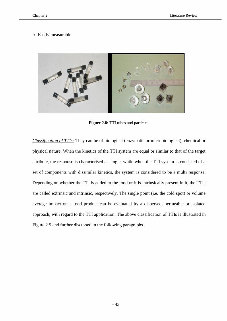
Chapter 2 Literature Review
- 43
o Easily measurable.
Figure 2.8: TTI tubes and particles.
Classification of TTIs: They can be of biological (enzymatic or microbiological), chemical or
physical nature. When the kinetics of the TTI system are equal or similar to that of the target
attribute, the response is characterised as single, while when the TTI system is consisted of a
set of components with dissimilar kinetics, the system is considered to be a multi response.
Depending on whether the TTI is added to the food or it is intrinsically present in it, the TTIs
are called extrinsic and intrinsic, respectively. The single point (i.e. the cold spot) or volume
average impact on a food product can be evaluated by a dispersed, permeable or isolated
approach, with regard to the TTI application. The above classification of TTIs is illustrated in
Figure 2.9 and further discussed in the following paragraphs.

Chapter 2 Literature Review
- 44
Figure 2.9: Classification of TTIs (Hendrickx et al., 1993).
Working principle of TTIs: The nature of the TTI system affects the time needed for post-
processing to obtain the process value at the end of the thermal treatment. Biological TTIs are
the most studied systems yet the post-processing is highly-time consuming, as the population
of the viable cells needs to be counted. However, the fact that they are heat sensitive over the
same temperature range as their target gives them a major advantage. Processes based on
enzymic TTIs are more advantageous since their denaturation enthalpy and activity can be
more easily and accurately measured and they are small enough to be used in a variety of
containers and processes. Microbiological systems need to be calibrated before being used to
any thermal treatment evaluation, as the microorganisms can exhibit inherent variability
(Pflug and Odlaug, 1987). Enzymatic TTI systems also need to be thoroughly calibrated due
to batch differences and storage conditions.
TTI systems of chemical nature are flexible and exhibit analytical precision, but they still
have not been applied to thermal processes.
Chapter 2 Literature Review
- 45
Response types of TTIs: TTIs have a single or multicomponent response, depending on
whether or not they have similar kinetics as their target attribute, respectively. In the case of
single response, a direct correlation between the TTI system and the target organism can be
obtained, whereas in the multicomponent case, knowledge of target’s time-temperature profile
is needed (Taoukis, 1999). Studies have been carried out for dealing with the multicomponent
response by statistically correlating the TTI behaviour with the safety or quality attributes for
given time-temperature profiles. The equations used correspond to specific conditions with
different kinetics, meaning that if another time-temperature set is needed, extrapolation will
be required which can lead to uncertainty and errors. Stoforos and Taoukis, (1998) suggested
that components with z-value higher and lower than that of the target organism should be
included when multicomponent TTIs are used. Despite its limitations, the complex system of
the multiple TTI components can be useful in targeting multiple targets with various z-values,
showing potential for further investigation.
Origin: With regard to their origin, the TTIs can be intrinsic or extrinsic. The former, is
dispersed in the food product and can be used for either to evaluate a single point in the
product, which is usually the cold spot, or the average volume, while the latter is added to the
food. Intrinsic TTIs are convenient, as there is no need for a monitoring device, but the fact
that they are mixed with the environment they are subjected to, can cause difficulties in
determining the kinetics of the TTI and the product, separately. That is the reason why the
extrinsic TTIs are encapsulated in a variety of materials that isolates them from the actual
food product and the surrounding environment. When TTIs are encapsulated, it is important
that the properties (thermal or mechanical) of the carrier material are determined. This is
particularly important in the case of aseptically processed liquid or particulate foods. In the
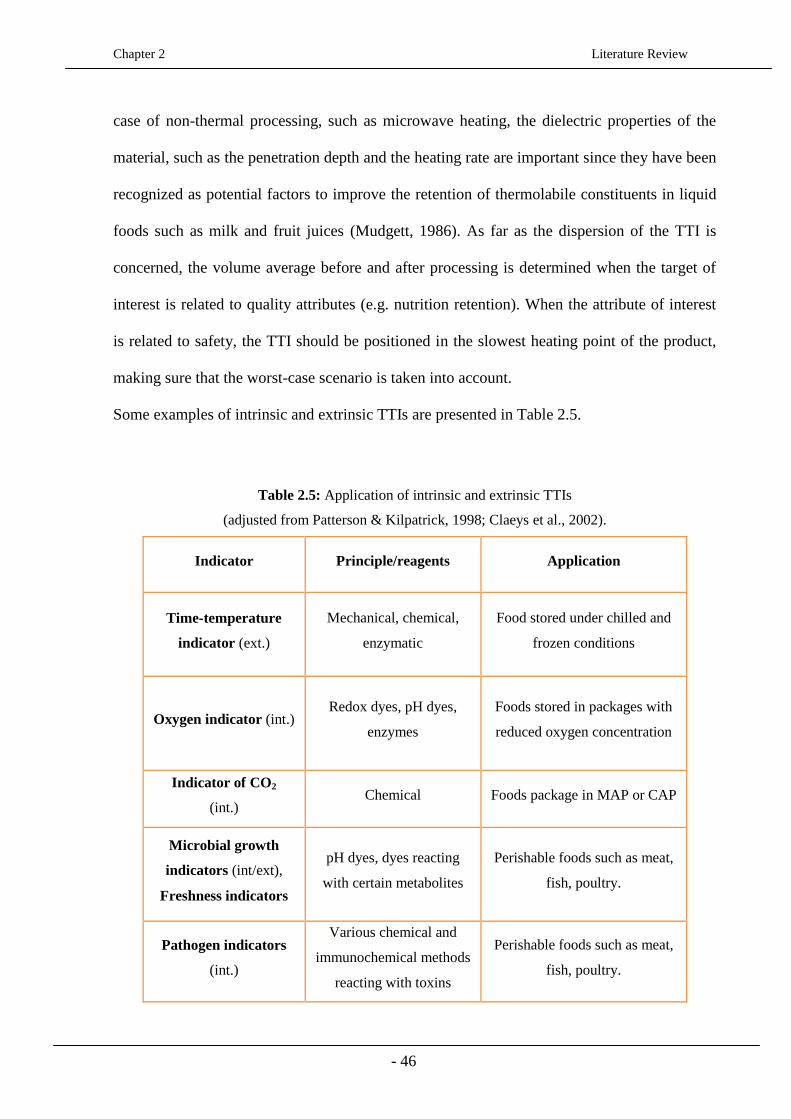
Chapter 2 Literature Review
- 46
case of non-thermal processing, such as microwave heating, the dielectric properties of the
material, such as the penetration depth and the heating rate are important since they have been
recognized as potential factors to improve the retention of thermolabile constituents in liquid
foods such as milk and fruit juices (Mudgett, 1986). As far as the dispersion of the TTI is
concerned, the volume average before and after processing is determined when the target of
interest is related to quality attributes (e.g. nutrition retention). When the attribute of interest
is related to safety, the TTI should be positioned in the slowest heating point of the product,
making sure that the worst-case scenario is taken into account.
Some examples of intrinsic and extrinsic TTIs are presented in Table 2.5.
Table 2.5: Application of intrinsic and extrinsic TTIs
(adjusted from Patterson & Kilpatrick, 1998; Claeys et al., 2002).
Indicator Principle/reagents Application
Time-temperature
indicator (ext.)
Mechanical, chemical,
enzymatic
Food stored under chilled and
frozen conditions
Oxygen indicator (int.) Redox dyes, pH dyes,
enzymes
Foods stored in packages with
reduced oxygen concentration
Indicator of CO2
(int.) Chemical Foods package in MAP or CAP
Microbial growth
indicators (int/ext),
Freshness indicators
pH dyes, dyes reacting
with certain metabolites
Perishable foods such as meat,
fish, poultry.
Pathogen indicators
(int.)
Various chemical and
immunochemical methods
reacting with toxins
Perishable foods such as meat,
fish, poultry.

Chapter 2 Literature Review
- 47
Application of TTIs: As already mentioned, TTIs have been used to monitor microorganisms
or enzymes with equal z-value (defined in § 2.2.1) or activation energy, when the time-
temperature profile of the food being heated is not known. Depending on the process targeted,
the range of z-values for the inactivation of vegetative pathogens, yeasts and mould lies in
between 5 and 12oC, which refers to pasteurisation processes, while for quality attributes,
such as vitamins and colour, it lies between 25 and 45oC (Lund, 1977). The canning process
applied in low-acid food products is based on the inactivation of Clostridium botulinum, with
a z-value of 10oC.
Most studies regarding TTI development are focused on enzymic and chemical TTIs, which
have been evaluated for their reliability and accuracy for a variety of thermal treatments, such
as pasteurisation and sterilisation, and semi-industrial processes in pilot plants. TTI systems
based on enzymes, originating from bacteria, such as α-amylases, are advantageous over other
biological TTI systems. They are convenient, as they are supplied in a powder form, they
undergo irreversible changes and they show first order reaction rate when exposed to high
temperatures, similar to the microbial destruction rate. Several types of enzymic TTIs have
been used to evaluate mild thermal processes; when it comes to more severe processes like
sterilisation, there is a limited number of enzymes resistant to temperatures >100oC. One such
enzyme that can potentially be used in sterilisation processes was isolated from a
hyperthermophilic microorganism, Pyrococcus furiosus. The amylase extracted is
thermostable and can survive throughout processes such as canning, batch vessels and ohmic
heating.
Potential TTI systems used in mild processes are reported in the literature. Extrinsic Bacillus
amyloliquefaciens α-amylase (BAA) based TTIs were used by Van Loey et al., (1996a) to
monitor pasteurisation processes with particulate foods and by Tucker et al., (2000) for the
Chapter 2 Literature Review
- 48
pasteurisation of fruit products in tubular heat exchangers and ohmic heating. Reyes de
Corcuera et al., (2005) studied the effectiveness of an exogenous, amperometric glucose
oxidase based TTI. The enzyme was entrapped in a thin film and positioned on the interior
wall of a capsule. The TTI system was investigated, under isothermal conditions for
temperatures 70 to 79.7oC, showing first order kinetics. Vaidya et al., (2003) investigated the
potential and effectiveness of a fluorescence emission based TTI system for the inactivation
of vegetative pathogens like Salmonella. The TTI were tested for temperatures ≥ 62.8oC and
showed good correlation between experimental and theoretical data. Another potential TTI
system used for the evaluation of pasteurisation processes was reported by Guiavarc’h et al.,
(2003); Pectinmethylesterases (PMEs), extracted from cucumber and tomatoes, were
subjected at a temperature range of 55–77oC with sugars or polyols being present. Cucumber
PMEs showed biphasic behaviour, while the tomato PMEs showed first order kinetics. Fruits
and vegetables can be a good source of enzymes, but the steps that need to be taken for
preparation and analysis can be time-consuming and excessive.
Enzymic TTIs have also been used for monitoring sterilisation processes. Bacillus
licheniformis α-amylase (BLA) based TTIs was used by Tucker et al. (2000) to evaluate
sterilisation processes and to investigate process value differences between freely moving and
fixed particles inside cans. Bacillus subtilis α-amylase based TTIs were used for evaluating
the end-over-end speed and viscosity influence in sterilised particulate foods (Van Loey et al.,
1997b). Spore distribution and leakage of Bacillus stearothermophilus spores was evaluated
using TTIs in an alginate-starch mushroom puree (Ocio et al., 1997), while Knap and
Durance, (1998) used the same spores to evaluate thermally processed particulate foods in an
agitating steam-air retort. Pilot plant studies have been carried out for both extrinsic and
intrinsic TTI systems, with Rodrigo et al. (1998) investigating the accuracy and performance
Chapter 2 Literature Review
- 49
of TTIs in a water immersion static retort and Hsu et al., (2000) using triose phosphate
isomerase for evaluating roast beef processing, respectively. Another application of the TTIs
was based on the formation of 2,3-dihydro-3,5dihydroxy-6-methyl-4(H)-pyran-4-one, for
prediction of the cooking effect in an ohmic heater (Eliot-GodeÂreaux et al., 2003).
Other types of TTIs that have been commercially used, include the CheckPoint® TTI
(VITSAB International AB, Malmo, Sweden) and the (eO) ®
TTI (CRYOLOG SA, France)
which are based on pH changes, caused by enzymatic hydrolysis and microbial growth,
respectively, expressed in colour changes. Other applications refer to TTIs used as active,
smart labels for monitoring time-temperature responses on food packages (e.g. on meals
served on flights). 3M Monitor Mark (3M Nederland B.V., Netherlands) is a diffusion-based
indicator label that monitors temperature exposure of temperature-sensitive products, such as
frozen or refrigerated foods during transportation and storage; the indicator monitors
temperature exposure, not product quality and it signals when the product quality should be
checked due to temperature exposure. Fresh-Check® (TEMPTIME Corporation, USA) is
another time temperature indicator, a self-adhesive device that is specifically formulated to
match the shelf life of the food products to which it is affixed. Its active centre circle darkens
irreversibly, faster at higher temperatures and slower at lower temperatures, indicating when
to USE or NOT USE the food product within the product date codes. As the active centre is
exposed to temperature over time it gradually changes colour to show the freshness of the
food product.
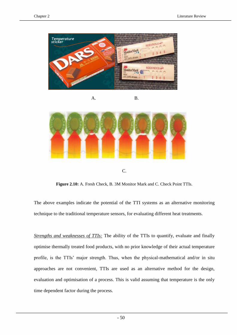
Chapter 2 Literature Review
- 50
A. B.
C.
Figure 2.10: A. Fresh Check, B. 3M Monitor Mark and C. Check Point TTIs.
The above examples indicate the potential of the TTI systems as an alternative monitoring
technique to the traditional temperature sensors, for evaluating different heat treatments.
Strengths and weaknesses of TTIs: The ability of the TTIs to quantify, evaluate and finally
optimise thermally treated food products, with no prior knowledge of their actual temperature
profile, is the TTIs’ major strength. Thus, when the physical-mathematical and/or in situ
approaches are not convenient, TTIs are used as an alternative method for the design,
evaluation and optimisation of a process. This is valid assuming that temperature is the only
time dependent factor during the process.

Chapter 2 Literature Review
- 51
The working principle of all types of TTIs is based on the calculation of the process value at
the beginning and the end of the thermal process, as their status changes (e.g. enzymic
activity). Thus, the online monitoring of the thermal process by the TTIs is not feasible, that
being their major weakness. The TTIs lack predictive power for processing conditions
different from the ones under which the experiments are run. Thus, the development of
mathematical models would overcome that problem and predict process times and
temperatures based on empirical formulae or theoretical heat transfer models. Based on
experiments from current work, modelling the heat process would potentially show by how
much the TTIs underestimate the process and what would the ideal process conditions for
following the thermocouples’ trend.
As described above, TTIs are classified according to their working principle, origin, type of
response, positioning and application mode, meaning that their strengths and weaknesses will
be relative and subject to the type of the TTIs used for different processes. The fact that the
TTIs are typically located on the product’s surface is another limitation of their use. The
temperature difference between the product and surface can be significantly different,
depending on product, package and process characteristics. Furthermore, different target
microorganisms and quality attributes would require different TTIs, making their application
even more challenging.
Recent work on TTIs: studies undertaken in recent years show the extended applicability of
TTIs. Claeys et al., (2002) used intrinsic TTIs (heat markers) to assess a high pressure
process. The results were not favourable for the use of TTIs at high pressure, but promising
for the further research. A TTI system consisted of an enzyme trapped in poly o-
phenylenediamine film, coated on the interior wall of a capsule (made of stainless steel) was

Chapter 2 Literature Review
- 52
studied by Reyes-De-Corcuera et al., (2005). The TTI system was subjected under
pasteurisation treatments and was analysed with an amperometer at the end of the treatment.
First order kinetics was followed with a z- value of 6˚C to 7˚C. The authors concluded that the
specific type of TTIs have the potential to validate pasteurisation processes, for targeting
E.Coli and Listeria monocytogenes. A number of studies and work has been done for
developing TTI systems that can assess sterilisation treatments; TTIs consisting α-amylase
from Bacillus subtilis and Bacillus licheniformis, have been studied the most (Tucker et al.,
2005b). Guiavarc'h et al., (2004a) showed that the Bacillus licheniformis based TTI with a z-
value of 9.4°C was able to monitor a sterilisation process at 121.1°C for up to 30 min, under
non isothermal conditions. The authors evaluated Bacillus subtilis and Bacillus licheniformis
TTI systems in an industrial application, where ravioli was processed in a continuous rotary
processing plant. TTIs were used together with thermocouples and were compared in terms
of process values. Bacillus licheniformis and Bacillus subtilis α – amylases showed z- values
of 13.9 and 16.4°C, respectively and were therefore (z-value> 10°C) used together as multi
component TTIs. The authors reported that the impact of the thermal process was
overestimated, causing food safety issues and that the use of the specific TTIs is complicated
in terms of preparation and analysis. TTIs made from Pyrococcus furiosus α-amylase, was
reported to be a better alternative for sterilisation processes (Tucker et al., 2005; Tucker et al.,
2007).
Mehauden et al., (2007) investigated the efficiency of an industrially scaled agitated vessel
under pasteurisation conditions, using Bacillus licheniformis a-amylase TTIs and
thermocouples for viscous model foods. The results showed that the process values obtained
by the TTIs were higher than the values of the thermocouples and therefore the TTIs
shouldn’t be used alone for assessing a thermal process, for safety reasons.

Chapter 2 Literature Review
- 53
Future trends: When the temperature history of the thermal process can be recorded and
controlled on-line, the physical-mathematical approach is preferred instead of the TTIs.
Neither of the approaches though, can derive direct measurement and be used as a predictive
tool. Thus, the development of predictive methods is essential. Ball, (1923); Ball and Olson,
(1957), developed such methods based on empirical/theoretical models constructed for heat
transfer predictions. Either temperature sensors are used, in the case of physical mathematical
approach, or an enzyme for TTI systems, calibration is a very important task for obtaining
accurate results. When predictive models are used accurate properties of the food product
processed, its surrounding environment and the packaging need to be determined.
By the use of predictive modeling the batches of food products that undergo process
deviation, would be able to be controlled and the process establishment would be more
straightforward (Tucker et al., 2003). Stoforos et al., (1997), refer to the TTI systems as an
essential complementary step in improving the physical-mathematical approach. Hence, a
future, improved plan of processing and design would associate the TTIs with temperature
sensors, each being included in a separate risk assessment procedure. The use of TTIs in
evaluating safety and/or quality attributes during heat processes or new technologies means
that they can also monitor critical control points, necessary in HACCP and be useful
companies’ demands on microbiological safety.
The reliability and accuracy of TTI systems, already investigated by a number of researchers,
will potentially lead to their application to the pharmaceutical and chemical industries, where
similar problems and risks to the food industry can be encountered. The development of the
various types of TTIs in combination or not with temperature sensors will provide a better
understanding of the new, non-thermal technologies that have been developed in the recent
years, ensuring safe, high quality foods and will help the food manufacturers to control and

Chapter 2 Literature Review
- 54
optimise their processes. Fryer and Robbins, (2005), report that the trajectories of the TTIs
need to be known in order to be able to use them for assessing heat treatments; that can be
achieved by the use of PEPT and PIV flow visualisation techniques.
In the current project, the hot-fill process is validated by a α-amylase based TTI system,
which is further discussed in Chapter 5.
2.3 Optimisation of thermal processes
The design and evaluation of thermal processes can be described by two methods; the General
and the Formula Method. The former originates from Bigelow et al., (1920) and is considered
to be very accurate, as it is based on experimental time-temperature data, but it lacks
predictive power. Formula methods have been used extensively since 1923 (Ball, 1923) and
combine kinetic and heat transfer models for describing the time dependence of temperature
within the product. Thus, for the optimisation of thermal processes, the heat transfer models
need to be combined with the kinetic ones (Figure 2.11).
The problems usually identified in optimising thermal processes, include the selection of the
design variables to be controlled, the constraints or assumptions made, the mathematical
equation used to describe what needs to be optimised and consequently the selection of the
proper mathematical model, and finally the choice of the optimisation technique. The
accuracy of the parameters chosen to be modelled is of great importance for optimising a
thermal process. Heat and mass transport phenomena, as well as the reaction kinetics of the
organisms targeted have to be considered.
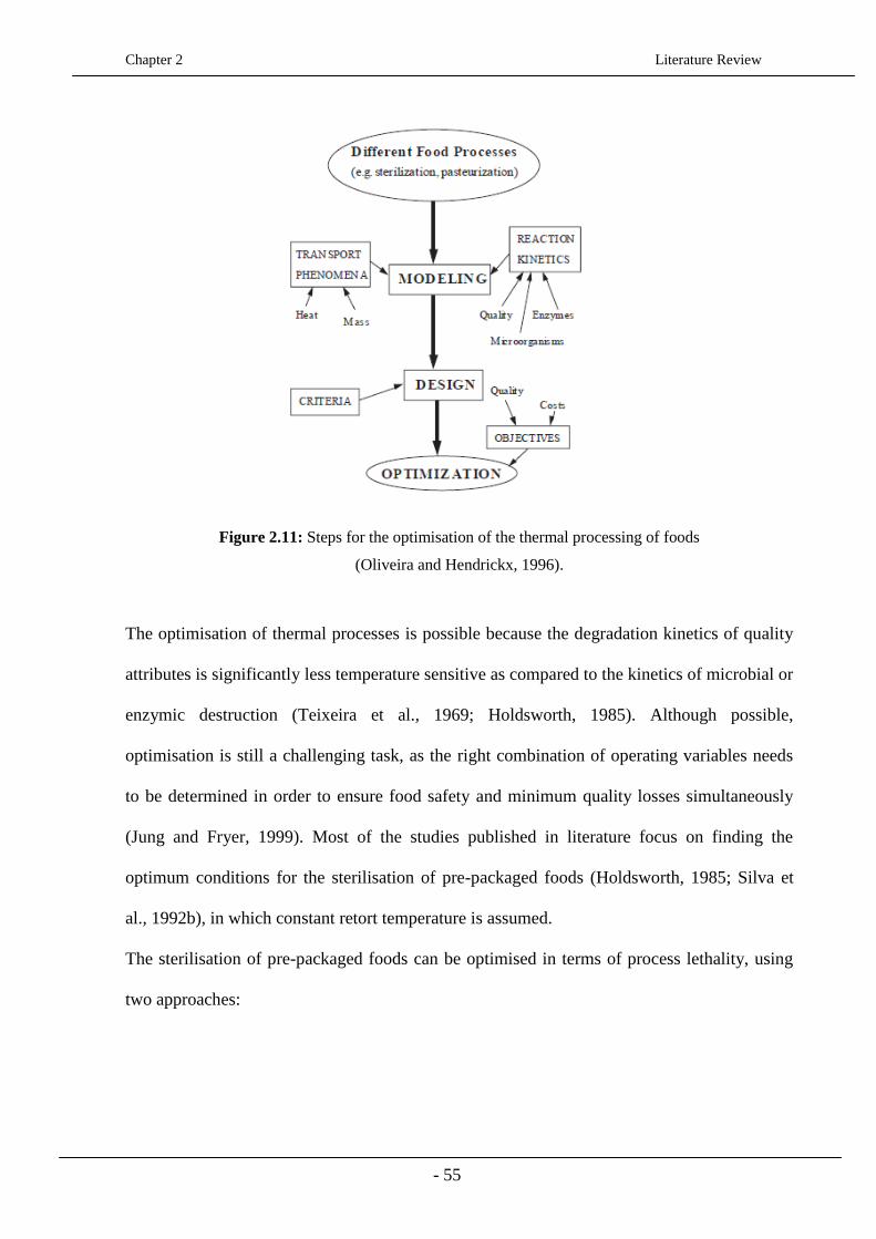
Chapter 2 Literature Review
- 55
Figure 2.11: Steps for the optimisation of the thermal processing of foods
(Oliveira and Hendrickx, 1996).
The optimisation of thermal processes is possible because the degradation kinetics of quality
attributes is significantly less temperature sensitive as compared to the kinetics of microbial or
enzymic destruction (Teixeira et al., 1969; Holdsworth, 1985). Although possible,
optimisation is still a challenging task, as the right combination of operating variables needs
to be determined in order to ensure food safety and minimum quality losses simultaneously
(Jung and Fryer, 1999). Most of the studies published in literature focus on finding the
optimum conditions for the sterilisation of pre-packaged foods (Holdsworth, 1985; Silva et
al., 1992b), in which constant retort temperature is assumed.
The sterilisation of pre-packaged foods can be optimised in terms of process lethality, using
two approaches:

Chapter 2 Literature Review
- 56
o The target lethality (Fo) at the coldest spot or least-lethality point (LLP), defined as
follows:
dtF
t
z
ToT
o
0
10 (2.1)
Where: T = temperature at any given time, To = reference temperature at 121.1oC and z =
10oC, based on the destruction of Clostridium botulinum on low-acid foods.
o The integrated lethality (Fs) that refers to the average volume of microbial survival
(Stumbo, 1973):
dV
VDF
V
FD
osoo
0
/110
1log (2.2)
Where: V = volume in m3, Do = D-value at To
The same equations can be used to describe quality attributes which are defined by the ‘cook
value’ (C-value) instead of the F-value for microbial inactivation, using the appropriate z-
value (Silva et al., 1994a). In the case of the target lethality approach, sensory parameters are
of interest, while the integrated lethality approach is more related to nutritional attributes
(Ohlsson, 1980a).
The target lethality determined at the slowest heating point (or LLP) of a cylindrical
container, is considered to be at its geometrical centre; however, this approach may not be
correct when including the cooling phase in the lethality calculation (Flambert and Deltour,
1972). According to Tucker and Clark, (1990) the cooling phase contributes significantly to
Chapter 2 Literature Review
- 57
the final sterility of products in rectangular containers. When the cooling phase is included in
the lethality calculations, the LLP is observed along the radius or vertical axis, depending on
the ratio of half-height to radius and the integrated lethality (Fs) approach needs to be used; if
measurements of single point are taken on the surface or the centre of the package, the process
will result in under-processing or over-processing, respectively.
Teixeira et al., (1969b) reported that the position of LLP depends on the geometry of the
container and the process conditions. Silva and Korczak (1994) also investigated the
localisation of the LLP for a product heated through conduction, in a finite cylindrical
container. They found that the kinetic parameters of the target organism, the processing
temperature, and the target lethality, have no impact on the LLP, while the dimensions of the
container and the product’s heating rate (surface resistance to heat transfer was taken into
account) influence it greatly. Flambert and Deltour, (1972) conducted similar experiments and
concluded that the LLP is only affected by the container’s dimensions, as surface resistance
was assumed negligible.
Silva et al., (1994) and Banga et al., (1993) validated the optimal quality conditions of pre-
packaged foods, experimentally; the degradation kinetics and the heat transfer mode into the
food were quantified and a quality indicator used. Finally, the best combination of processing
variables was chosen and compared to predicted values. The above study is based on the
validation of model foods and consequently the parameters taken into consideration are
heating by pure conduction, and regular geometries. Information on optimisation of realistic
conditions such as irregular geometries, particulate foods or conventional heated foods, is
limited. As far as mild heat treatments such as pasteurisation or hot-fill treatments are
concerned, there is very limited information on the optimisation of processing conditions.
Silva et al., (1997) developed a mathematical model, using a finite difference method, to
Chapter 2 Literature Review
- 58
describe the hot-fill treatment of fruit purees. Sandoval et al., (1994) predicted the time-
temperature profile of hot-filled tomato paste that was air-cooled, using analytical solutions.
Glass jars of 0.2, 0.5 and 4 L were hot-filled at 94, 92 and 90°C, respectively, and evaluated
for achieving inactivation of Bacillus coagulans. The same pasteurisation value of a process
can be achieved by several combinations of filling temperature, package size, heating medium
properties, etc., but only one pair of conditions can result in optimum quality retention of the
fruit preserved. Efforts to generate minimal quality losses of thermally processed foods have
been made for a long time, and several studies have been carried out on the development of
quality optimisation models (Silva et al., 1994; Fryer et al., 2008). The fact that the
degradation kinetics of quality attributes, such as nutrients, texture, colour, or flavour, are less
heat-sensitive than the kinetics related to the destruction of microorganisms or inactivation of
enzymes (Teixeira et al., 1969; Lund, 1977; Holdsworth, 1985), makes the optimisation
possible. Few studies about quality optimisation of foods have been reported in literature. Van
Loey et al., (1993) studied the impact of sterilisation on white beans in brine, while Banga et
al., (1993) used canned tuna. Kiranoudis and Markatos (2000) used a multi‐objective design
and a static mathematical model to optimise food dryers. The authors aimed to minimize an
economic measure and the colour deviation of the final product, simultaneously. Olmos et al.,
(2002) considered the constraint approach as a compromise between the process time and the
quality of the final product. The approach aims at maximising the final product quality
repeatedly subject to a total drying time constraint, which is varies in each optimisation.
Chapter 2 Literature Review
- 59
2.3.1 Kinetic models
The kinetic models can predict the time-temperature dependence of safety or quality
attributes, assuming that accurate reaction kinetics of microbial destruction, enzymic
inactivation or quality degradation, depending on the organism targeted, is obtained.
Theory of Microbial Deactivation by Heating
The reactions involved in any thermal process are affected by the contribution of the heating,
holding and cooling period to the process. The overall effect (lethality) is determined by
evaluating the three different periods individually, as the contribution of each one is
significantly different, depending on the process. For instance, when rapid heating and
cooling are required, the most important period is the holding period, which will affect the
final lethality the most. The temperature during the holding period is constant, which makes it
relatively easy to determine the reaction rates of microbial destruction; it is the most
convenient period to deal with. The destruction rates have to be observed as a function of
temperature. Determining the temperatures at which the various organisms are inactivated, is
of great importance in thermal processes. Different microorganisms exhibit different
temperature sensitivity, with vegetative pathogens, yeasts and moulds being the most
susceptible ones and the endospores being the most resistant ones (e.g. Bacillus
stearothermophilus, B. subtilis, or B. cereus; and B. stearothermophilus and Cl.
Thermosaccharolyticum present in milk and fruits, respectively); viruses lie in between
(Johnson et al., 1982; Maggi et al., 1997; Gaze and Brown, 1998). Enzymes, either
intracellular or extracellular, also have different temperature resistance and need to be
inactivated while the nutritional components are retained (Holdsworth, 1992).

Chapter 2 Literature Review
- 60
The surrounding medium of the microorganisms, particularly the pH and aw, and the type and
concentration of components the food product is consisted of (e.g. fats, carbohydrates), have
substantial impact on the growth of microorganisms. The pH and aw-value of the medium is
mostly associated with the growth of vegetative microorganisms (Brown & Booth, 1991) and
has a tremendous impact on microbial death. For example, the vegetative bacteria present in
products like butter, are much more resistance than in aqueous environments, such as juices
(Herson & Hulland, 1980). The rate of microbial death or quality degradation as a time and
temperature function is required in order to evaluate thermal processes. The destruction of
microorganisms is assumed to be a first-order reaction, which means that at constant
temperature, the rate of the target organism is proportional to its concentration at the
particular time. According to the first-order kinetics theory, at a defined time, the number of
microorganisms will reduce to the one-tenth of the population at the start of that time interval,
regardless of the actual population. In essence, at a constant lethal temperature and after each
time interval the number of microorganisms will be reduced by 90% of the original number.
Figure 2.12 shows the remaining number of the living cells after each time interval.
Figure 2.12: Microbial death curve at constant lethal temperature (Lewis, 2000).
Chapter 2 Literature Review
- 61
The amount of time, in minutes, required for heating a microorganism at a constant lethal
temperature, to cause a ten-fold reduction in the number initial living cells, is referred to as
The Decimal Reduction Time (DRT). The lethal constant temperature at which the food is
subjected to, is the temperature at which microorganisms begin to die. In other words, DRT is
the time needed for the spores of a particular food to be reduced by 90%, at a specific
temperature. Thus, after a 1D reduction, only 10% of the original spores will survive. It has
been accepted that the decrease in the number of microorganisms is nearly logarithmic, as a
function of time (Anderson, 1996). The remaining number of organisms can never be zero;
there is a finite chance of survival. That chance needs to be reduced to an acceptable level,
depending on the food product and the target process, ensuring that the product delivered to
the consumer will be free of spoilage microorganisms. The units of the food product that are
to be produced and the initial population of microorganisms within it need to be taken into
consideration in order to establish the acceptable level of survival.
In low acid foods, pH>4.5, where the target organism is the heat-resistant spore-forming
Clostridium botulinum, the commercially acceptable level of survival is 1 in 1012
, which
means that in an initial spore population of 1012
, only 1 spore will survive the thermal process.
The Cl. botulinum survival rate of 1012
, which is generally known as the 12D concept, has
been alternatively defined in the United Kingdom, as the chance of survival of 1 spore of Cl.
botulinum in 1012
containers rather than 1012
initial spores. In any case, the 12D concept is
also referred to as a Fo3 process, and was proposed by Stumbo (1965). A Fo3 process means
that at a constant reference temperature of 121.1oC, 3 minutes are needed for Cl. botulinum to
be inactivated. The 12-log reduction of the Cl. Botulinum spores does not necessarily ensure
commercial sterility of the product, as other non-pathogenic bacteria, that are more heat-
Chapter 2 Literature Review
- 62
resistant, higher D-value, may be still active; in that case, a more severe heat treatment is
required, which involves either higher processing temperatures or an additional heating step.
Microorganisms that show higher thermal resistance than Cl. botulinum are the thermophilic
spores, which can grow at ambient temperatures. Their acceptable level of survival lies
between 105 and 10
7 (5D to 7D reduction), assuming that this still results in a 12D reduction
for Cl botulinum (Madigan, 2006).
The microbial death by heat can be mathematically expressed by the following equation, in
terms of concentration of microorganisms (C):
Ckdt
dC (2.3)
Where: t is the given time, and k is the constant reaction rate
At the different times, t1 and t2, at the same temperature the respective concentration of
organisms C1 and C2 is given by integrating Equation 2.3:
12
2
1ln ttkC
C (2.4)
By substituting the concentration C of microorganisms with the actual number N present
within a container, can be more useful. Thus, Equation 2.4 can be written as follows:
12
2
1ln ttkN
N (2.5)
Or
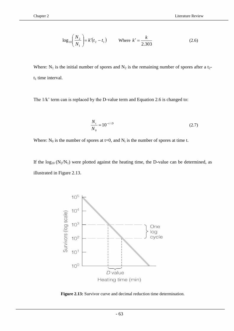
Chapter 2 Literature Review
- 63
12
1
2
10log ttkN
N
Where
303.2
kk (2.6)
Where: N1 is the initial number of spores and N2 is the remaining number of spores after a t2-
t1 time interval.
The 1/k’ term can is replaced by the D-value term and Equation 2.6 is changed to:
Dtt
N
N /
0
10 (2.7)
Where: N0 is the number of spores at t=0, and Nt is the number of spores at time t.
If the log10 (N2/N1) were plotted against the heating time, the D-value can be determined, as
illustrated in Figure 2.13.
Figure 2.13: Survivor curve and decimal reduction time determination.

Chapter 2 Literature Review
- 64
When the temperature of the process is increased, the rate at which microorganisms or
enzymes are inactivated increases as well and according to Equation 2.5 the decimal reduction
time will decrease. The effect of temperature on decimal reduction time has been described by
the z-value model and the Arrhenius equation model. The latter has been mostly used to
describe the temperature effect on chemical reactions, and data extrapolation is usually
required (Jonsson, 1977; Pflug, 1996; Fujikawa, 1998).
In the current project, the temperature effect was described by the z-value model, according to
which, when temperature is raised by z degrees C, the decimal reduction time is changed by a
factor of 10. Thus, the z-value is the temperature required for achieving a 1-log reduction in
the D-value and it is related to the resistance of the microorganism to different temperatures.
Bigelow, (1920) showed that there is a linear relationship between the temperature and the
logarithm of the D-value; when plotted, the reciprocal of the slope, gives the z-value.
The logarithm of D-values against temperature is illustrated in Figure 2.14 and the curve
obtained, is called a thermal death time (TDT) curve; important for calculations required for
thermal destruction of microorganisms. The linear slope of the TDT curve shows the
temperature sensitivity of the target microorganism. The time–temperature combinations
obtained from the points along the TDT line, give equal lethal effect for a given
microorganism. Consequently, the z-model, using the D- and z-value constants, can
characterise adequately the temperature resistance of safety and quality attributes.
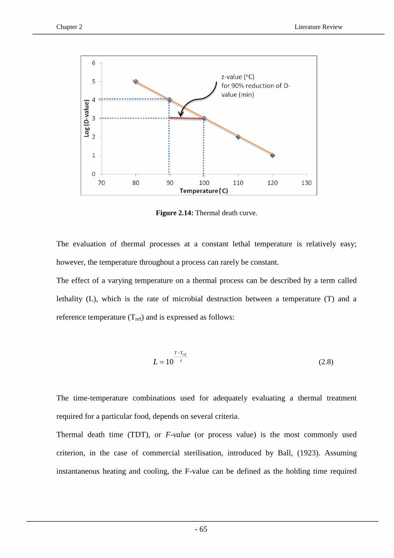
Chapter 2 Literature Review
- 65
Figure 2.14: Thermal death curve.
The evaluation of thermal processes at a constant lethal temperature is relatively easy;
however, the temperature throughout a process can rarely be constant.
The effect of a varying temperature on a thermal process can be described by a term called
lethality (L), which is the rate of microbial destruction between a temperature (T) and a
reference temperature (Tref) and is expressed as follows:
z
TT ref
L
10 (2.8)
The time-temperature combinations used for adequately evaluating a thermal treatment
required for a particular food, depends on several criteria.
Thermal death time (TDT), or F-value (or process value) is the most commonly used
criterion, in the case of commercial sterilisation, introduced by Ball, (1923). Assuming
instantaneous heating and cooling, the F-value can be defined as the holding time required

Chapter 2 Literature Review
- 66
achieving thermal destruction of microorganisms, at a constant reference temperature and is
described by the following equation:
dtdtLF
t
z
TTt ref
00
10 (2.9)
The process value (F and P-value for sterilization and pasteurization, respectively) can be
determined either by being based on the time-temperature history knowledge, or on
measurements of the initial (No) and final (Nf) loads of the organism present. The process
value is expressed in the following equation:
dtN
NDPorF
t
z
TT
f
T
reft
0
0 10log (2.10)
Where: T (t) is the product temperature at the slowest heating point (°C), Tref is the reference
temperature (°C), t is the process time (min) and z is the value of the temperature required for
a 1D reduction and should be the one of the target organism.
When the target organism refers to enzymes, Equation 2.8 is changed to:
dtA
ADPorF
t
z
TT
f
T
reft
0
0 10log (2.11)
Where: Ao and Af, are the initial and final enzyme activity, respectively.
Chapter 2 Literature Review
- 67
Besides from the criteria used to characterise the thermal destruction of microorganisms, there
are other that are based on biochemical degradation or cooking of a food product. Whatever
the target and the criteria used, the reference temperature used should be close to the process
temperature, for avoiding data errors (e.g. extrapolation at higher temperatures).
The thermal process criterion should be referred to the organisms most likely to survive the
process. For instance, when Cl. botulinum is the organism of interest, the Fo (at a Tref of
121.1oC and z-value of 10
oC) value is the appropriate one, but in the case of other surviving
organisms the process value F should be based on their z-value.
2.3.2 Mathematical Models
As mentioned in the previous sections, thermal processing is widely used in the food industry
for ensuring safety and delivering quality final products. Foods are complex matrices with
varying rheological and thermo-physical properties. They are time and process dependent and
therefore it is difficult to make accurate prediction of the process they are involved in (Fryer
et al., 2005). Thermal processing of many solid foods is based upon heat and moisture transfer
between the solid body and the heating medium. A number of heat transfer mathematical
models, based on quantification of heat and mass transfer phenomena have been developed
for predicting temperature variation as a function of operating variables, at any location and
time (Balsa-Canto et al., 2002a). Most heat transfer models are developed for describing the
sterilisation treatment. The requirements imposed to sterilisation processes, which depend on
the objectives that need to be satisfied, can be determined analytically or numerically. Both
approaches have been used in a number of studies dealing with conduction and convective
heated foods, for predicting the time-temperature, velocity, pressure profiles, and fluid flow

Chapter 2 Literature Review
- 68
behaviour throughout the process. Models referring to conduction heated foods, such as tuna,
thick syrups and purees are based on the assumption that the product is heated by pure
conduction, it is homogeneous, there is negligible surface resistance to heat transfer, the
heating medium temperature is constant and the geometry of the contained is considered to be
cylindrical (Perrota, 2011). Complexities during conduction heated foods occur due to the
polymorphic nature of food components (Fryer, 2005).
Most commercially processed food products are heated by a combination of conduction and
convection; the widely used heat process of canning is one such example. Heat within the can
is transferred by a combination of conduction and natural convection. In the case of sterilised
liquid foods, both conduction and natural convection have significant effect in heat transfer.
Datta et al., (1988); Varma and Kannan, (2006) studied natural convection in canned liquid
foods and used numerical solutions to predict transient temperature and velocity profiles.
They reached the conclusion that the slowest heating point is observed at approximately the
one tenth of the can’s bottom. Kumar and Bhattacharya, (1990) studied the sterilisation of
viscous, canned liquid foods heated from the side walls, keeping the bottom and top surfaces
insulated. Keeping the thermal properties of the liquid food constant and assuming
temperature dependent viscosity, the authors found that the slowest heating point moved
towards the can’s bottom due to natural convection occurrence.
Processing liquid foods is complex due to fluid motion and consequently their simulation is
also complicated; equations of continuity, energy and momentum need to be solved
simultaneously and more complex boundary conditions need to be considered (Ghani et al.,
1999). Owing to the complexity of describing the sterilisation of liquid foods mathematically,
equations that include dimensionless parameters, such as Ra, Nu, Re, and Pr number, have
been developed (Sablani, 2006).

Chapter 2 Literature Review
- 69
Regardless of the heat transfer mechanism occurring during thermal processing of foods,
either analytical and/or numerical methods can be used.
2.3.2.1 Analytical methods
They are exact solutions of differential equations that are important for the design and
optimisation of a process that includes solid food products with simple geometries, such as
infinite slab, cylinder, or sphere (Ramaswamy et al., 1984). Laplace transform and separation
of variables are included in the solutions, with the latter being used in heat conduction
problems with homogeneous boundary and initial conditions (Özisik, 1993). The validation of
numerical solutions with uniform boundary conditions and constant thermal properties is a
typical application of analytical solutions (Cai et al., 2003).
2.3.2.2 Numerical methods
They are used when analytical solutions are not available; they have the advantage of being
flexible, dealing with irregular geometries, complex boundary conditions and temperature
dependent thermal properties, but they are not exact solutions. Numerical methods are useful
for estimating the thermal behaviour of foods under complex but realistic conditions such as
variation in initial temperature, non-linear and non-isotropic thermal properties, irregular-
shaped bodies and time dependent boundary conditions (Puri & Anantheswaran, 1993).
Numerical modelling technology is a powerful and efficient tool for simulating thermal
processes in the food industry (Ahmad & Okos, 2001).
For developing a mathematical model, the problem to be solved needs to be described, to be
formulated mathematically and discretised choosing the appropriate numerical solution. The
solution is finally visualised and the problem is ideally approximated (Figure 2.15).

Chapter 2 Literature Review
- 70
Figure 2.15: Solving a mathematical model (Martin Burger, 2010).
Finite difference, finite element and finite volume methods have widely been used for
numerically solving models associated with food processing (Fryer et al., 1995; Erdogdu et
al., 1998a; Sun et al., 2000a).
Each method is summarised in the following paragraphs.
Finite Difference method (FD)
The FD method is commonly used for simple geometries such as slab, cylinder and sphere; it
can be applied to two or three-dimensional problems and involves simple boundary conditions
with constant thermal diffusivity. The method has been widely used to solve heat and mass
transfer models of thermal processes such as cooking and frying (Erdogdu et al., 1998a, Pan
et al., 2000), drying (Thorvaldsson & Janestad, 1999), and cooling (Chuntranuluck et
al.,1998a, b, c). FD method has been used to model the heating process of liquid-solid
Chapter 2 Literature Review
- 71
systems in processes such as blanching, sous-vide and sterilisation (Farkas et al., 1996b;
Wang & Chen, 1999; Davey & Pham, 1997) The heat transferred through a solid food product
is described by Fourier’s equation of heat conduction, whilst the interaction between the
liquid and the solid is considered in the boundary conditions. Fasina & Fleming, (2001)
described the heat transfer through a cucumber, during the blanching process using an axi-
symmetric, two dimensional FD heat conduction model, assuming a cylinder shape. Ghazala
et al., (1995) used FD method to predict the time-temperature history of sous-vide processed
fish and meat products of rectangular shape. The convective heat transfer coefficient of the
surface is very large and therefore, the authors assumed that its effect on the temperature
profiles of the food was negligible. Thus, the heat transfer coefficient was arbitrarily set at a
high value during the simulation of a three-dimensional FD heat conduction model. Solid
particle foods sterilised in a container with a brine solution is another example of liquid-solid
heat process modelled with the FD method. Akterian (1995, 1997) used a one-dimensional
model to determine the temperature distribution of canned mushrooms in brine.
The FD method has proved not to be satisfactory for temperature predictions on foods with
irregular shapes due to geometric simplification (Coulter et al., 1995; Russell, & James, 1996;
Ansari et al., 1999).
Finite Element method (FE)
The FE method has been reported to perform better for irregular geometries and complex
boundary conditions than the FD method (Van Der Sluis et al., 1994; Carroll et al., 1996).
The FE method concerns the discretisation of a domain into a number of small elements; the
developed element equations are then assembled for the whole domain, and solved (Zhao et
al., 1998; Wang & Sun, 2003). The discretisation of the differential equations is based on the
Chapter 2 Literature Review
- 72
interpolation of polynomials in order to describe the variation of a field variable within an
element (Rao, 1989). The FE method has been successfully used to solve heat and mass
transfer models for cooking (Evans & Warboys, 1997; Wang et al., 1999), drying (Ahmad et
al., 2001; Jia et al., 2000a, 2001) and cooling (Van Der Sluis & Rouwen, 1994; Carroll et al.,
1996; Wang & Sun, 2002a, b).
FE method has been used to simulate microwave heating of a solid food of cylindrical and
rectangular shape (Lin et al., 1995). The authors expressed the microwave power density
absorbed at any location within the food product, as a function of the dielectric properties and
food geometry; the surface heat losses by convection and evaporation were in the boundary
conditions. Zhou et al., (1995), reported that in the case of high amount of moisture loss, a
coupled heat and mass transfer model needs to be used, implicating at the same time Fick’s
law for the moisture transfer through the solid.
FE approach was also used for modelling the process of microwave drying for heat-sensitive
foods, such as biscuits (Lian et al., 1997; Ahmad et al., 2001). The prediction of temperature
and moisture distribution of regular shaped chicken patties, in an air-convection heating oven
was shown to be better predicted by the FE for a coupled heat and mass transfer model, as
compared to heat transfer model used alone (Chen et al., 1999). A coupled heat and mass
transfer FE model with inner heat generation was also used for the modelling of cooked meat
joints in commercial vacuum cooling (Wang & Sun, 2002a, 2003). FE scheme has also been
used for modelling convection heated foods. Thermal processes such as sterilisation of canned
liquid and spray drying of liquid or powder foods, like in the case of starch dispersion have
been predicted using coupled fluid flow and heat transfer models (Yang & Rao, 1998;
Straatsma et al., 1999; Verboven et al., 2000a, b). Tewkesbury et al., (2000) used a FE model
to predict the cooling of chocolate; the conduction occurring during the cooling phase of
Chapter 2 Literature Review
- 73
chocolate and the change in specific heat capacity of the product, were modelled as a function
of temperature and cooling rate.
A commercial finite element program (FIDAP) has been used by a few authors for simulating
processes with complex liquid food systems. The program was used by Kumar and
Bhattacharya (1991a) for calculating the lethality of a shear thinning, temperature dependent
viscosity fluid along the centreline, whilst Jung and Fryer (1999) used it for estimating the
lethality and quality of both a Newtonian and shear thinning fluid in terms of bulk averages.
Later, Liao et al., (2000) used the same program to determine the lethality at the slowest
heating point of a processed starch suspension.
Despite its advantages, the FE method is complex and computationally expensive, as
compared to the FD method.
Finite Volume/Computational Fluid Dynamics (CFD)
CFD is a simulation tool for solving fluid flow and heat transfer problems. The energy
conservation, continuity and momentum equation are solved simultaneously to predict
velocity, temperature, pressure profiles, and other fluid flow parameters in a system (Sun,
2002). CFD has been mainly applied to automotive and nuclear industries but has been
recently used into the food industry. Applications of CFD in the food industry include air flow
analyses in ovens and chillers (Foster et al., 2002), fluid flow of particle foods in processing
systems (Mirade & Daudin, 2000), convection flow patterns in containers during sterilisation
processes (Ghani et al., 1999a, b), and modelling of vacuum cooling processes (Sun & Hu,
2003).
The heat treatment of solid foods in industrial convection ovens, such as hot-air electrical
forced convection ovens, can be modelled as a coupled fluid flow and heat transfer problem;
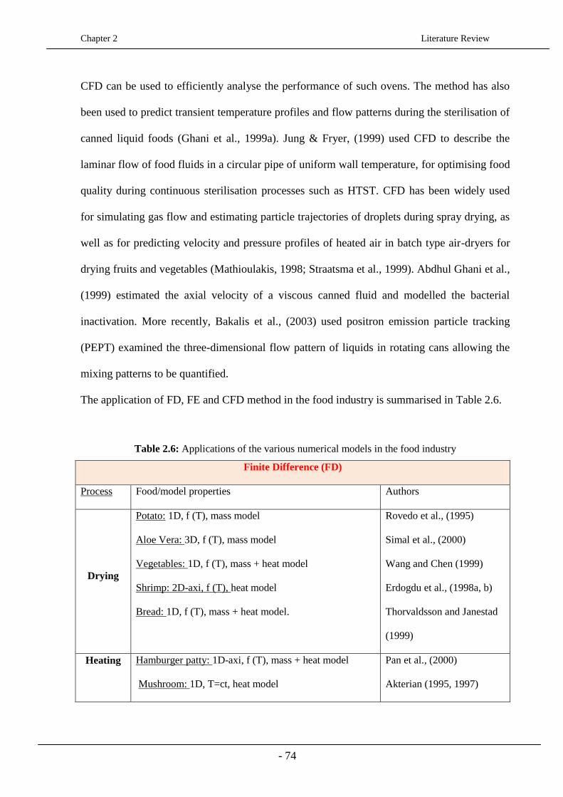
Chapter 2 Literature Review
- 74
CFD can be used to efficiently analyse the performance of such ovens. The method has also
been used to predict transient temperature profiles and flow patterns during the sterilisation of
canned liquid foods (Ghani et al., 1999a). Jung & Fryer, (1999) used CFD to describe the
laminar flow of food fluids in a circular pipe of uniform wall temperature, for optimising food
quality during continuous sterilisation processes such as HTST. CFD has been widely used
for simulating gas flow and estimating particle trajectories of droplets during spray drying, as
well as for predicting velocity and pressure profiles of heated air in batch type air-dryers for
drying fruits and vegetables (Mathioulakis, 1998; Straatsma et al., 1999). Abdhul Ghani et al.,
(1999) estimated the axial velocity of a viscous canned fluid and modelled the bacterial
inactivation. More recently, Bakalis et al., (2003) used positron emission particle tracking
(PEPT) examined the three-dimensional flow pattern of liquids in rotating cans allowing the
mixing patterns to be quantified.
The application of FD, FE and CFD method in the food industry is summarised in Table 2.6.
Table 2.6: Applications of the various numerical models in the food industry
Finite Difference (FD)
Process Food/model properties Authors
Drying
Potato: 1D, f (T), mass model
Aloe Vera: 3D, f (T), mass model
Vegetables: 1D, f (T), mass + heat model
Shrimp: 2D-axi, f (T), heat model
Bread: 1D, f (T), mass + heat model.
Rovedo et al., (1995)
Simal et al., (2000)
Wang and Chen (1999)
Erdogdu et al., (1998a, b)
Thorvaldsson and Janestad
(1999)
Heating
Hamburger patty: 1D-axi, f (T), mass + heat model
Mushroom: 1D, T=ct, heat model
Pan et al., (2000)
Akterian (1995, 1997)

Chapter 2 Literature Review
- 75
Heating
Cucumber: 2D-axi, f (T), heat model
Carcases: 1D, f (T), heat model
Sauce: 1D, T=ct, heat model
Fasina and Flemiung (2001)
Coulter et al., (1995);
Davey and Pham (1997)
Evans et al., (1996)
Cooling
Frozen foods: 3D, f (T), heat model
Potato: 1D-axi, T=ct, heat model
De Elvira et al., (1996)
Chavez et al., (1996)
Finite Element (FE)
Drying
Grain: 2D-axi, f (T), mass + heat model
Biscuits: 2D-axi, f (T), mass + heat model
Chicken: 2D-axi, f (T), heat model
Starch: 2D, f (T), mass + heat model
Jia et al., (2000a,b,c,d, 2001))
Ahmad et al., (2001)
Chen et al., (1999)
Wu and Irudayaray (1996);
Yang and Rao (1998).
Heating
Solid foods: 1D-axi, f (T), mass + heat model
Broccoli: 1D-axi, f (T), heat model
Carcases: 2D, f (T), heat model
Apple and Pear: 1D, f (T), heat model
Lin et al., (1995);
Vilayannur et al., (1998a,b);
Varga et al., (2000)
Martens et al., (1996)
Mallikarjunan and Mittal
(1994, 1995)
Carroll et al., (1996)
Cooling
Various: 2D, heat model
Cooked meats: 2D-3D, f (T), mass + heat model
Bakery products: 3D, f (T), mass + heat model
Chocolate: 2D-axi, f (T), heat model
Comini et al., (1995)
Wang and Sun
(2002a,b,c,d,e)
Van Der Sluis and Rouwen
(1994, 1999).
Tewkesbury et al., (2000)

Chapter 2 Literature Review
- 76
Computational Fluid Dynamics (CFD)
Drying
Particle food: f (T), mass + heat model
Fruits & Vegetables: f (T), mass model
Various
Straatsma et al., (1999)
Mathioulakis et al., (1998)
Verboven et al., (2000a,b)
Heating
Canned liquid food: heat model
Vegetables: f (T), mass model
Various: f (T), mass+heat model
Ghani et al., (1999a,b, 2001)
Tassou and Xiang (1998)
Jung and Fryer (1999)
Cooling Various: 3D, f (T), mass+heat model
Particulated foods: 2D-3D, mass+heat model
Cooked meats: mass model
Cortella et al., (2001)
Xu and Burfoot (1999a,b)
Hu and Sun (2000, 2001a,b,
2002)
Continuous progress has been made in recent years for improving the accuracy of the
developed mathematical models, but more research still needs to be carried out on:
More accurate estimations of surface heat and mass transfer coefficients (De Elvira et al.,
1996; Nicolai et al., 2000);
Food properties and their interactions;
Sensitivity analysis for judging assumptions such as temperature and thermal properties of
foods (Nicolai et al., 1999; Oliveira, 2000; Verboven et al., 2001).
2.4 Conclusions
In recent years, the increased variety of food products and the consumers’ awareness of food
safety and quality have led food manufacturers to be faced with the challenge of producing
safe and high quality food products. A number of food preservation techniques, such as
Chapter 2 Literature Review
- 77
thermal and low temperature processing, dehydration, irradiation or a combination of them is
applied in order to satisfy the consumers’ demands. The common working principle of all
processes is the inactivation of microbial growth whilst ideally minimising the physical
damage and the possibility for undesirable chemical reactions (Dewanto, 2002).
Thermal processing is the most widely used and well established preservation method in food
industry. The application of heat serves a number of objectives, with safety being the primary
one; quality is another important reason for heating food products. The degree, at which both
safety and quality are affected during heating, is subject to the intensity of the process applied,
with sterilisation being the most severe one.
For ensuring safety of the final product, inactivation of the spoilage organisms on the food
product alone is not sufficient; package decontamination is equally important (Tucker et al.,
2002). The decontamination method applied on the container is dependent on the food target;
it can be thermal (application of steam), chemical (e.g. hydrogen peroxide, ethylene oxide),
radiation (e.g. UV, IR) or a combination of them.
In order to establish a safe thermal process, accurate validation needs to be performed.
Temperature probes and loggers, and microbiological methods are the most widely applied
monitoring techniques. The continuously increasing variety of food products has led to the
development of novel, more sophisticated validation techniques. Retort simulators, thermal
imaging technology and time temperature integrators are such examples.
The ultimate goal of food processing is achieving safety and the highest quality possible at the
same time for the final product. For optimising thermal processes the reaction kinetics of the
safety and/or quality attributes need to be known in combination with information on the mass
and heat transport phenomena occurring during the process applied.
Chapter 2 Literature Review
- 78
The kinetic models are used to predict the time-temperature dependence of safety or quality
attributes and are expressed in terms of lethality; the mathematical models used, intend to
predict the dependence of operating variables as a function of temperature distribution by
quantifying heat and mass transfer behaviour during the process (Balsa-Canto et al., 2002a).
The progress made during the last decades in optimising thermal processes has been
exponential, since the models used have predictive power and can be combined with
analytical methods. However, more research needs to be carried out in obtaining deeper
understanding of food properties, more accurate estimates of heat and mass transfer
coefficients, more sensitive and practical validation techniques and further studying of novel
processes.
The current work covers the inversion step as a thermal treatment of the headspace and lid for
hot-filled products. The effectiveness of the step in terms of heat transfer enhancement during
the cooling phase of the process was simulated and combined with analytical solutions.
Kinetic models were used and compared with the simulated models, for validating the
process.
References
Adams M. R., Moss M.O., (2007). Food Microbiology. New Age International.
Agency for Toxic Substances and Disease Registry (ATSDR), (1990). Toxicological Profile
for Ethylene Oxide. U.S. Public Health Service, U.S. Department of Health and Human
Services, Atlanta, GA.
Ahmad S.S., Morgan M.T., Okos M.R., (2001). Effects of microwave on the drying, checking
and mechanical strength of baked biscuits. Journal of Food Engineering, 50, 63–75.
Chapter 2 Literature Review
- 79
Akterian S.G., (1995). Numerical simulation of unsteady heat transfer in canned mushrooms
in brine during sterilisation processes. Journal of Food Engineering, 25, 45–53.
Akterian S. G., (1997). Control strategy using functions of sensitivity for thermal processing
of sausages. Journal of Food Engineering, 31, 449–455.
Alzamora S.M., Tapia M.S., Welti-Chanes J., (2003). The control of water activity. Food
Preservation Techniques, Woodhead Publishing, Cambridge, 126-153.
Amann, R.I., Ludwig, W., Schleifer, K.-H., (1995). Phylogenetic identification and in situ
detection of individual microbial cells without cultivation. Microbiol. Rev., 59, 143 – 169.
Anderson W.A., McClure P.J., Baird Parker A.C., Cole, M.B., (1996). The application of a
log-logistic model to describe the thermal inactivation of Cl. botulinum 213B at temperatures
below 121.1oC. Journal of Applied Bacteriology, 80, 283-290.
Anonymous, (1995). Determination of moisture content in Finnish honey using an
infrareddryer. Food Market Technology, 9(1), 40–41.
Anonymous, (2007a). Almonds grown in California; outgoing quality control requirements.
Federal Register. Agricultural Marketing Service, USDA, 72 (61), 15021–15036.
Ansari F.A, (1999). Finite difference solution of heat and mass transfer problems related to
precooling of food. Energy Conversion & Management, 40, 795–802.
Ansari M.I.A., Datta A.K., (2003). An overview of sterilisation methods for packaging
materials used in aseptic packaging systems. Trans IChemE, 81, 57-65.
Ávila I.M.L.B., Silva C.L.M., (1995). Optimum sterilisation conditions for foods inside packs
with two divisions. Poster presented at: 9th World Congress of Food Science and Technology,
Budapeste (Hungary).
Bachmann R., (1975). Sterilisation by intense ultraviolet radiation. The Brown Boveri Rev. 62,
206-209.
Bajgai T. R., Hashinaga E., (2001). High electric field drying of Japanese radish. Drying
Technol. 19, 2291-2302.
Ball C.O. (1923). Thermal Process Time for Canned Food, Bulletin of the National Research
Council, Washington, DC. Vol. 7, Part 1, Number 37.
Ball C.O. and Olsen, F.C.W. (1957). Sterilization in Food Technology. McGraw-Hill Book
Co., New York.
Balsa-Canto E., Banga, J.R, Alonso A.A., (2002). A novel, efficient and reliable method for
thermal process design and optimization. Part II: Applications Journal of Food Engineering
52 (3), 235-247.

Chapter 2 Literature Review
- 80
Bakalis S., Cox P.W., Wang-Nolan W., Parker D.J., Fryer P.J. (2003). Use of Positron
Emission Particle Tracking (PEPT) technique for velocity measurements in model food fluids,
Journal of Food Science, 68, 2684–2692.
Banga J.R., Balsa-Canto E., Moles C.G., Alonso A.A., (2003). Improving food processing
using modern optimization methods. Trends in Food Science & Technology, 14(4), 131–144.
Barbosa-Canovas G.V., Qin, B.L., Pothakamury, U.R., Swanson B.G., (1996). Non-thermal
pasteurization of liquid foods using high-intensity pulsed electric fields Crit. Rev. Food
Science and Nutrition, 36, 603–627
Barrett D.M, (2006). Maximizing the nutritional value of fruits and vegetables. Review of
literature on nutritional value of produce compares fresh, frozen, and canned products and
indicates areas for further research.
http://www.fruitandvegetable.ucdavis.edu/files/197179.pdf
Barsotti L., Merle P. P., Cheftel J., (1999). Food processing by pulsed electric fields: Physical
aspects. Food Review International, 15(2), 163-180.
Bauser M., Sauer G., Siegert K., (2006). Extrusion, ASM International, p. 270.
Bazhal M.I., (2001). Etude du mecanisme d'electropermeabilisation des tissus vegetux.
Application ii l'extraction du jus des pommes, These de Doctorat, Universite de Technologie
de Compiegne, France.
Bee G.R., Park D.K., (1978). Heat-penetration measurement for thermal-process design. Food
Technology, 32(6): 56-58.
Berry B.W., (2000). Use of infrared thermography to assess temperature variability in beef
patties cooked from the frozen and thawed states. Foodservice Research International, 12(4),
255–262.
Bigelow W.D., Bohart G.S., Richardson A.C., Ball C.O., (1920). Heat penetration in
processing canned foods. Bull. Nr 16-L Res. Washington, D.C.: Lab. Natl. Canners Assn.
Bongiovanni R., Lowenberg-Deboer J., (2004). Precision agriculture and sustainability.
Precision Agriculture, 4(4), 359–387.
Boonsupthip W., Heldman D.R., (2007). Prediction of frozen food properties during freezing
using product composition. Journal of Food Science, 72 (5), 254-263.
Bown G., (2003). Developments in conventional heat treatment. Food preservation
Techniques, Woodhead Publishing, Cambridge, 154-178.
Brown A.C., (2007). Understanding Food: Principles and Preparation (3 ed.). Cengage
Learning

Chapter 2 Literature Review
- 81
Brown K.L., Ayres, C.A., Gaze, J.E., Newman, M.E., (1984). Thermal destruction of bacterial
spores immobilised in food/alginate particles. Food Microbiology, 1, 187-198.
Brown M.H., Booth, I.R., (1991). Acidulants and low pH. In Food Preservatives, pp. 2243.
Edited by N. J. Russell & G. W. Gould. Glasgow & London: Blackie.
Bruhn C.M., (1995). Strategies for communicating the facts on food irradiation to consumers.
J. Food Protect., 58, 213–216.
Burfoot D., Mulvey E., Foy E., Turner R., Bayliss D., McFarland S., Jewell K. (2014). Food
surface decontamination to improve food safety and extend shelf life. Campden BRI R&D
report no. 358.
Codex Alimentarius Commission (CAC), (1994). Codex General Standard for Irradiated
Foods and of untreated and radiation-damaged Listeria as affected by Recommended
International Codex of Practice for the Opera- environmental factors. Acta Microbiology and
Immunology Hung. 42, Radiation Facilities used for the Treatment of Food. 19–28. CAC/Vol.
XV.-Ed.1. FAO, Rome.
Cai R., Zhang N., (2003). Explicit analytical solutions of 2-D laminar natural convection.
International Journal of Heat Mass Transfer, 26, 931–934.
Campbell P., Braam J., (1999). In vitro activities of four xyloglucan endotransglycosylases
from Arabidopsis. Plant Journal, 18, 371–382.
Carroll N., Mohtar R., Segerlind L.J., (1996). Predicting the cooling time for irregular shaped
food products. Journal of Food Process Engineering, 19, 385–401.
Council of Agricultural Science and Technology (CAST), (1995). Food Borne Illnesses:
Risks and Consequences. Report No. 122.
Castro I., Macedo B., Teixeira J. A., Vicente A. A. (2004). The effect of electric field on
important food-processing enzymes: Comparison of inactivation kinetics under conventional
and ohmic heating. Journal of Food Science, 69, 696–701.
Campden & Chorleywood Food Research Association (CCFRA), (1977). Guidelines to the
establishment of scheduled heat processes for low-acid foods, CCFRA Technical Manual
No.3.
Campden & Chorleywood Food Research Association (CCFRA), (2006b). Pasteurisation: A
food industry practical guide (second edition). Guideline No.51.
Campden & Chorleywood Food Research Association (CCFRA), (2007). Guidelines for the
processing of aseptic packaging Guideline 53.
Campden & Chorleywood Food Research Association (CCFRA), (2011). Energy efficiency
by thermal imaging. Brewing analysis leaflet Gary Freeman.
Chapter 2 Literature Review
- 82
Campden & Chorleywood Food Research Association (CCFRA), (2012). Surface
decontamination: A review. Confidential internal publication
Campden & Chorleywood Food Research Association (CCFRA), (2014). Microbiological
safety and quality of chilled pasteurised food products: A review. G Betts.
Cho H.Y., Yousef A.E., Sastry S.K., (1996). Growth kinetics of Lactobacillus acidophilus
under ohmic heating. Journal of Biotechnology and Bioengineering, 5, 49(3), 334-340.
Chuntranuluck S., Wells C.M., Cleland A.C., (1998a). Prediction of chilling times of foods in
situations where evaporative cooling is significant: Method development. Journal of Food
Engineering, 37, 111–125.
CODEX, (1997). Hazard Analysis and Critical Control Point (HACCP) System and
Guidelines for Its Application Annex to CAC/RCP 1-1969, Rev. 3.
Chapman S., (2003). New machines use tumbling process to decontaminate food. Food
Chem. News, 10:20.
Chen H.Q., Marks B.P., Murphy R.Y., (1999). Modelling coupled heat and mass transfer for
convection cooking of chicken patties. Journal of Food Engineering, 42, 139–146.
Cho H.Y., Yousef A.E., Sastry S.K., (1996). Growth kinetics of Lactobacillus acidophilus
under ohmic heating. Journal of Biotechnology and Bioengineering, 5, 49(3), 334-340.
Claeys W.L., Van Loey A.M., Hendrickx, M.E., (2002). Intrinsic time temperature integrators
for heat treatment of milk. Trends Food Science Technology, 13, 293-311.
Coulter S., Pham Q.T., McNeil I., McPhail, N.G., (1995). Geometry, cooling rates and weight
losses during pig chilling. International Journal of Refrigeration, 18, 456–464.
Datta A.K., Teixeira A.A., (1988). Numerically predicted transient temperature and velocity
profiles during natural convection heating of canned liquid foods. Journal of Food Science, 53
(1), 191-195.
Davey L.M., Pham Q.T., (1997). Predicting the dynamic product heat load and weight loss
during beef chilling using a multi-region finite difference approach. International Journal of
Refrigeration, 20, 470–482.
De Cordt S., Hendrickx M., Maesmans G., Tobback P., (1992). Immobilised -amylase from
Bacillus licheniformis: a potential enzymic time-temperature integrator for thermal
processing. International Journal of Food Science and Technology, 27, 661-673.
De Elvira C., Sanz, P.D., Carrasco, J.A., (1996). Characterising the detachment of thermal
and geometric centres in a parallelepipedic frozen food subjected to a fluctuation in storage
temperature. Journal of Food Engineering, 29, 257–268.

Chapter 2 Literature Review
- 83
Dostie M., Seguin J.N., Maure D, Tonthat Q.A., Chatingy R., (1989). Preliminary
measurements on the drying of thick porous materials by combinations of intermittent
infrared and continuous convection heating. New York, Hemisphere Press.
Dewanto V., Wu X., Kafui K. Adom, Liu R. H., (2002). Thermal Processing Enhances the
Nutritional Value of Tomatoes by Increasing Total Antioxidant Activity. Journal of
Agriculture and Food Chemistry, 50, 3010−3014
Dunn J., (2015). Pulsed Light and Pulsed Electric Field for Foods and Eggs, Oxford Journals.
Science & Mathematics Poultry Science, 75(9), 1133-1136.
Eliot-Godereaux S., Goullieux A., Queneudec T’kint M., (2003). Elaboration and kinetic
modelling of the formation of a biochemical marker to quantify HTST processing. Food
Research International, 36, 131-139.
Erdogdu F., Balaban M. O., Chau, K. V., (1998a). Modelling of heat conduction in elliptical
cross section: I. Development and testing of the model. Journal of Food Engineering, 38,
223–239.
Estiaghi M.N., Knorr D., (1999). Method for treating sugar beet. International Patent Nr WO
99/6434.
Evans J., Russell S., James S., (1996). Chilling of recipe dish meals to meet cook-chill
guidelines. International Journal of Refrigeration, 19, 79–86.
Evans R., Warboys M., (1997). Coupled heat and moisture during microwave vacuum drying.
Journal of Microwave Power and Electromagnetic Energy, 32, 34–44.
FAO., (1984a). Food aid in figures. FAO, Rome, p.118.
Farkas J., Andrassy E ., Meszaros L., Reichart O., (1996). Effect of radiation damage on the
apparent lag phase of Listeria monocytogenes. 16th International Symposium of the ICFMH,
p. 158.
Farkas B.E., Singh R.P., Rumsey T.R., (1996b). Modelling heat and mass transfer in
immersion frying. II, model solution and verification. Journal of Food Engineering, 29, 227–
248.
Farkas J., (1998). Irradiation as a method for decontaminating food. International Journal of
Food Microbiology, 44, 189–204.
Farkas J., (1999). Radiation processing: an efficient means to enhance the bacteriological
safety of foods. New Food, 2, 31-33.
Fasina O.O. Fleming H.P., (2001). Heat transfer characteristics of cucumbers during
blanching. Journal of Food Engineering, 47, 203–210.
Chapter 2 Literature Review
- 84
Food and Drug Administration (F.D.A), (1997). Irradiation in the production, processing and
treatment in vacuum packaged ground pork. Fed. 59, 1164–1166, Registry 62, 64102–64121.
Fellows P.J., (2000). Food Processing Technology: Principles and Practice, second ed., CRC
Press, New York.
Fenton G.A., Kennedy M.J., (1998). Rapid dry weight determination of kiwifruit pomace and
apple pomace using an infrared drying technique. New Zealand Journal of Crop and
Horticulture Science, 26, 35–38.
Flambert E., Deltour J., (1972). Localization of the critical area in thermally-processed
conduction heated canned food. Lebensm-Wiss U. Technology, 5(1), 7.
Floros J.D., Ozdemir M., Nelson P.E., (1998). Trends in aseptic packaging and bulk storage.
Food Cosmetics and Drug Packaging, 21, 236–239.
Floros J.D., (1993). Aseptic packaging technology: Principles of aseptic processing and
packaging (2nd ed.). Washington, DC: Food Processors Institute, p 115–48.
Floros J., (2008). Food science: feeding the world. Food Technol, 62(5), 11.
Formanek Z., Kerry J.P., Galven K., Buckey D.J., Farkas J., (1996). Effect of dietary vitamin
E supplementation and post slaughter addition of rosemary extract on oxidative stability of
irradiated minced beef. 42nd ICOMST, Lillehammer, Norway, p. 90–91.
Foster A.M., Barrett R., James S.J., Swain M.J., (2002). Measurement and prediction of air
movement through doorways in refrigerated rooms. International Journal of Refrigeration,
25, 1102–1109.
Fryer P.J., (1995). Electrical resistance heating of foods: New Methods of Food Preservation.
Blackie Academic & Professional, London.
Fryer P.J., (1997). Thermal treatment of foods. In P.J. Fryer, D.L. Pyle, and C.D. Rielly
(Eds.). Chemical engineering for the food industry, 331-382. London, Blackie A & P.
Fryer, P. J., Robbins P.T., (2005). Heat transfer in food processing: ensuring product quality
and safety. Applied Thermal Engineering, 25(16), 2499–2510.
Fryer P.J., Simmons M.J.H., Mehauden K., Bakalis S., (2008). Validation of thermal
processing using time temperature indicators as process probes. Journal of Food Engineering,
9 (1), 33-42.
Fujikawa H., Itoh T., (1998). Thermal inactivation analysis of mesophiles using the Arrhenius
and z-value models. Journal of Food Protection, 7, 785-923, 910-912(3).
Gagnon M., Abdellaoui S., Lacroix M., Jobin M., Boubekri C., (1995). Effect of gamma
irradiation combined with hot water treatment on the physico-chemical, nutritional and

Chapter 2 Literature Review
- 85
organoleptic qualities of clementines., International Journal of Food Science and Technology,
15, 217-235.
García M.J., Acinas S.G., Antón A.I., Rodríguez V.F., (1999). Use of the 16S–23S ribosomal
genes spacer region in studies of prokaryotic diversity. Journal of Microbiological Methods,
36, 55–64.
Ghani A.G.A., Farid, M.M., Chen, X.D., Richards P., (1999). Numerical simulation of natural
convection heating of canned food by computational fluiddynamics. Journal of Food
Engineering, 41, 55–64.
Ghazala S., Ramaswamy H.S., Smith J.P., Simpson M.V., (1995). Thermal process simulation
of sous-vide processing of fish and meat foods. Food Research International, 28, 117–122.
Gaze J.E., Brown K.L., (1998). The heat resistance of spores of Clostridium botulinum 213B
over the temperature range 120 8C to 140 8C. International Journal of Food Science and
Technology, 23, 373 – 378.
Giovannoni S.J., Britschgi T.B., Moyer C.L., Field K.G., (1990). Genetic diversity in
Saragasso Sea Bacterioplankton. Nature, 345, 60-62.
Gould G.W., (1989). Heat Induced Injury and Inactivation in Mechanisms of Action of Food
Preservation Procedures: Safe at the plate. Nutrition Today, 12(6), 6–9, 28–31.
Gracias K.S., McKillip J.L., (2004). A review of conventional detection and enumeration
methods for pathogenic bacteria in food. Canadian Journal of Microbiology, 50(11), 883-890.
Guiavarc‟h Y., (2003). Development and use of enzymic time-temperature integrators for the
assessment of thermal processes in terms of food safety. PhD Thesis No.570, Katholike
Universiteit Leuven, Belgium.
Guiavarc'h Y., Van Loey A., Zuber F., Hendrickx M., (2004a). Development characterization
and use of a high-performance enzymatic time-temperature integrator for the control of
sterilization process' impacts. Biotechnology and Bioengineering, 88, 15-25.
Gupta M.J., Irudayaraj J.M., Debroy C., Schmilovitch Z., Mizrach A., (2005). Differentiation
of food pathogens using FTIR and artificial neural networks. Trans. ASAE., 48, 1889-1892.
Hagen W, Drawert F., (1986). Determination of water content by infrared. Monatsschrift
Brauwissenschaft, 40(6), 240–246.
Hall M.J., Ratledge C., (1977). Applied and Environmental Microbiology, 34, 230.
Hammer K.A., Carson C.F., Riley T.V., (1999). Journal of Applied Microbiology, 86, 985–
990.
Han J.H., Floros J.D., (2007). Active packaging: a non-thermal process: Advances in thermal
and non-thermal food preservation. Ames: Blackwell Publishing, p 167–83.
Chapter 2 Literature Review
- 86
Head I.M., Saunders J.R., Pickup R.W., (1998). Microbial evolution, diversity, and ecology: a
decade of ribosomal analysis of uncultivated microorganisms. Microbiology and Ecology, 35,
1 – 21.
Heldman D.R., Hartel R.W., (1997). Principles of food processing. New York: Chapman &
Hall, p.288.
Hendrickx M., Maesmans G., De Cordt S., Noronha J., Tobback P., (1993). The evaluation of
the integrated time-temperature effect in thermal processing of foods. Critical Reviews in
Food Science and Nutrition.
Hendrickx M., Maesmans G., De Cordt S., Noronha J., Van Loey A., Tobback P., (1995).
Evaluation of the integrated time-temperature effect in thermal processing of foods. Critical
Reviews in Food Science & Nutrition, 35 (3), 231-262.
Heppell N.J., (1985). Measurement of the liquid-solid heat transfer coefficient during
continuous sterilisation of liquids containing particles. Symposium, Aseptic Processing and
Packaging of Foods, Tylosand, Sweden, p.108.
Herson A.C., Hulland, E.D., (1964). Canned Foods, an Introduction to their Microbiology
(Baumgartner), 5th ed. Chem. Pub. Co. Inc., New York.
Herson A.C., Hulland E. D., (1980). Canned Foods. Thermal Processing and Microbiology.
Holdsworth S.D., (1985). Optimisation of thermal processing review, Journal of Food
Engineering, 4, 89-116.
Holdsworth S.D., (1992). Aseptic processing and packaging of food products. Elsevier
Science Publishers Ltd.
Holdsworth S.D., (1997). Thermal processing of packaged foods. Blackie Academic &
Professional, London.
Hsu Y.C., Sair A.I., Booren A.M., Smith, D.M., (2000). Triose phosphate isomerise as an
endogenous time temperature integrator to verify adequacy of roast beef processing, Journal
of Food Science, 65(2), 236-240.
Icier F., Ilicali C., (2005a). The effects of concentration on electrical conductivity of orange
juice concentrates during ohmic heating. European Food Research and Technology, 220,
406–414.10.
International Commission on Microbiological Specification for Foods (ICMSF), (1996).
Microorganisms in foods: Characteristics of microbial pathogens. 5, p. 513.
IFT Food Technology, (2007). 61, 40–44
Chapter 2 Literature Review
- 87
International Life Sciences Institute, (ILSI), (2004b). Nutritional and safety assessments of
foods and feeds nutritionally improved through biotechnology: an executive summary.
Journal of Food Science, 69:CRH62–8.
James M. Jay, (1995). Food Preservation with Chemicals Modern Food Microbiology. Food
Science Texts Series, p. 273-303.
Jia C.C., Sun D.W., Cao C.W., (2000a). Mathematical simulation of temperature and moisture
fields within a grain kernel during drying. Drying Technology, 18, 1305–1325.
Jia C.C., Sun D.W., Cao C.W., (2001). Computer simulation of temperature changes in a
wheat storage bin. Journal of Stored Products Research, 37, 165–177.
Jorge C. Oliveira, Hendrickx M.E., (1996). Process Optimisation and Minimal Processing of
Foods. COPERNICUS PROGRAMME Concerted action, CIPA-CT94-0195.
Johnston M. D., Lawson S., Otter, J. A., (2005). Evaluation of hydrogen peroxide vapour as a
method for the decontamination of surfaces contaminated with Clostridium botulinum spores.
Journal of Microbiological Methods, 60 (3), 403-411.
Johnson A.D., Barka A., Mertz J.E., (1982). Nucleotide sequence analysis of the
recombination joints in 16 naturally-arising deletion mutants of SV40. Virology, 464–469.
Jonsson U., Snygg B.G., Harnulv, B.G., Zacrisson T., (1977). Testing two models for the
temperature dependence of the heat inactivation rate of Bacillus stearothermophilus spores.
Journal of Food Science, 42, 1251-1252.
Jung A., Fryer, P.J., (1999). Optimising the quality of safe food: computational modelling of a
continuous sterilisation process. Chemical Engineering Science, 54, 717–730.
Kader A.A., (2005). Increasing food availability by reducing postharvest losses of fresh
produce. 5th International Postharvest Symposium Acta Hortic., 682, ISHS 2005.
Kim T., Silva J., Chen T., (2002). Effects of UV irradiation on selected pathogens in peptone
water and on stainless steel and chicken meat. Journal of Food Protection, 65 (7): 1142-1145.
King C.J., (1968). Rates of sorption and desorption in porous, dried foodstuffs. Food
Technology, 22, 165–171, 509.
Kiranoudis C., Markatos N., (2000). Pareto design of conveyor-belt dryers. Journal of Food
Engineering, 46, 145–155.
Knap R.P., Durance T.D., (1998). Thermal processing of suspended food particles in cans
with end-over-end agitation. Food Research International, 31(9), 635-643.

Chapter 2 Literature Review
- 88
Kumar A. Bhattacharya, M. Blaylock J., (1990). Numerical simulation of natural convection
heating of canned thick viscous food products. Journal of Food Science, 55, 1403–1411,
1420.
Kumar A., Bhattacharya M., (1991a). Numerical analysis of aseptic processing of a non-
Newtonian liquid food in a tubular heat exchanger. Chemical Engineering Community, 103,
27–51.
Lacroix M., Ouattara B., (2000). Combined industrial processes with irradiation to assure
inequity and preservation of food products: a review. Food Research International, 33(9),
719–724.
Larousse J., Brown B.E., (1997). Food Canning Technology, 235-264, 297-332, 383-424,
489-530, New York: Wiley-VCH
Lee S., (2004). Microbial Safety of Pickled Fruits and Vegetables and Hurdle Technology.
Internet Journal of Food Safety, 4, 21–32.
Leistner L., (1995). Principles and applications of hurdle technology: New Methods of Food
Preservation. Springer, 1-21.
Leizerson S., Shimoni E., (2005). Effect of ultrahigh-temperature continuous ohmic heating
treatment on fresh orange juice. Journal of Agricultural and Food Chemistry, 53, 3519–3524.
Lewis M.J., Heppell, N.J., (2002). Continuous Thermal Processing of Foods: Pasteurization
and UHT Sterilization. Journal of the Science of Food and Agriculture, 82(4).
Lian G., Harris C.S., Evans R., Warboys M., (1997). Coupled heat and moisture transfer
during microwave vacuum drying. Journal of Microwave Power and Electromagnetic
Energy, 32, 34–44.
Liao H.J, Rao M.A., Datta A.K., (2000). Role of thermo-rheological behaviour in simulation
of continuous sterilization of starch dispersion. Trans. IChemE., 78, C, 48–56.
Lioliou E.E., Pantazaki A.A., Kyriakidis D.A., (2004). Thermus thermophilus genome
analysis: benefits and implications. Microbial Cell Factories, 3:5.
Lin Y.E., Anantheswaran R.C., Puri V.M., (1995). Finite element analysis of microwave
heating of solid foods. Journal of Food Engineering, 25, 85–112.
Ludwig W., Schleifer K.H., (1994). Bacterial phylogeny based on 16S and 23S rRNA
sequence analysis. FEMS Microbiological Rev. 15, 155 – 173.
Lund D.B., (1975). Heat processing: Physical Principles of Food Preservation. Marcel
Dekker, New York.
Chapter 2 Literature Review
- 89
Mathioulakis E., Karathanos V.T., Belessiotis V.G., (1998). Simulation of air movement in a
dryer by computational fluid dynamics: application for the drying of fruits. Journal of Food
Engineering, 36, 183–200.
McKenna A.B., Tucker G.S., (1991). Computer modelling for the control of particle
sterilization under dynamic flow conditions. Food Control, 2, 224-233.
Madigan M.T., Martino J.M., (2006). Brock Biology of Microorganisms (11th ed.). Pearson,
p. 136.
Maesmans G., Hendrickx M., De Cordt S., Van Loey A., Noronha J., Tobback P. (1994).
Evaluation of process value distribution with time temperature integrators. Food Research
International, 27, 413-423.
Maggi P., Carbonara S., Fico C., Santantonio T., Romanelli C., Sforza E., Pastore G., (1997).
Epidemiological, clinical and therapeutic evaluation of the Italian cholera epidemic in Europe.
Journal of Epidemiology, 13, 95–97.
Marquenie D., (2003). Combinations of pulsed white light and UV-C or mild heat treatment
to inactivate conidia of Botrytis cinerea and Monilia fructigena. International Journal of Food
Microbiology, 85 (1-2), 185-196.
Marquis R. E., Baldec, J., (2007). Sporicidal interactions of ultraviolet irradiation and
hydrogen peroxide related to aseptic technology. Chemical Engineering and Processing, 46
(6), 547-553.
Mattsson B., Sonesson U., (2003). Environmentally-friendly food processing. United
Kingdom: Woodhead Publishing Limited, p. 337.
Miller J.J., (1989). Sporulation in Saccharomyces cerevisiae. Academic Press, New York, 3,
p. 489-541.
McGee Harold, (2004). Wood Smoke and Charred Wood. On Food and Cooking .Scribner,
p. 448–450.
Meade S.J., Reid E.A., Gerrard J.A., (2005). The impact of processing on the nutritional
quality of food proteins. Journal AOAC International, 88, 904–922.
Mehauden K., Cox P.W., Bakalis S., Simmons M.J.H., Tucker G.S., Fryer P.J., (2007). A
novel method to evaluate the applicability of time-temperature integrators to different
temperature profiles. Innovative Food Science & Emerging Technologies, 8, 507-514.
Mirade P.S., Daudin J.D., (2000). Numerical study of the airflow patterns in a sausage dryer.
Drying Technology, 18, 81–97.
Mongpreneet S., Abe T., Tsurusaki T., (2002). Accelerated drying of welsh onion by far
infrared radiation under vacuum conditions. Journal of Food Engineering, 55, 147–156.
Chapter 2 Literature Review
- 90
Monroe J.J., Loessner M.J., Allen G.D., (2005). Modern Food Microbiology, Springer.
Montville T.J., Matthews K.R., (2005). Food microbiology an introduction. American Society
for Microbiology Press, p. 30.
Mossoba M.M., Al-Khaldi S.F., Kirkwood J., Fry F.S., Sedman J., Ismail A.A, (2005).
Printing microarrays of bacteria for identification by infrared micro spectroscopy. Vibrational
Spectroscopy, 38, 229-235.
Mudgett R.E., (1986). Electrical properties of foods: Engineering properties of foods. p. 329–
390. New York, NY: Marcel Dekker, Inc.
Muyzer G., (1999). DGGE/TGGE a method for identifying genes from natural ecosystems.
Current Opinions in Microbiology. 2, 317 – 322.
NACMCF, (2010). Reports and Recommendations Study of Microbiological Criteria as
Indicators of Process Control or Insanitary Conditions.
Nanjundaswamy A.M., Saroja S., Ranganna S., (1973). Determination of thermal process for
canned mango products. Indian Food Packer 27(6), 5.
Nath N., Ranganna S., (1983b). Determination of a thermal process schedule for guava
Psidium guajava Linn. Food Technology, 18, 301-316.
NAS, (1973). Toxicants occurring naturally in foods. Committee on Food Protection.
Washington, DC: National Academy of Sciences, p. 624.
Navari P., Andrieu J., Gevaudan A., (1992). Studies on infrared and convective drying of no
hygroscopic solids. Drying 92, Amsterdam: Elsevier Science. p. 685–94.
Nelson P.E. (1993). Principles of Aseptic Processing and Packaging (3rd ed.). p. 101-133.
Newsome R., Fisher W., (2007). Feeding the World Today and Tomorrow: The Importance of
Food Science and Technology. An IFT Scientific Review by John D. Floros.
Nicolai B.M., De Baerdemaeker J., (1999). A variance propagation algorithm for the
computation of heat conduction under stochastic conditions. International Journal of Heat
and Mass Transfer, 42, 1513–1520.
Nicolai B.M., Scheerlinck N., Verboven P., De Baerdemaeker J., (2000). Stochastic
perturbation analysis of thermal food processes with random field parameters. Transactions of
the ASAE, 43, 131–138.
Nowak D., Levicki P.P., (2004). Infrared drying of apple slices. Innovative Food Science
Emerging Technologies, 5, 353–360.
Chapter 2 Literature Review
- 91
Ocio M.J., Salvador Fernandez P, Rodrigo M., Periago P., Martinez A., (1997). A time
temperature integrator for particulated foods: thermal process evaluation. Food Research and
Technology, 205(4), 325-328.
Ohlsson, (1980a). Optimal sterilisation temperatures for flat containers, Journal of Food
Science, 45, 848-853.
Olmos A., Trelea I.C., Courtois F., Bonazzi C., Trystram G., (2002). Dynamic optimal control
of batch rice drying process. Drying Technology, 20(7), 1319–1345.
Ozdemir M., Floros J.D., (2004). Active food packaging technologies. CRC Critical Review
in Food Science and Nutrition, 44(3),185–193.
Özisik M.N., (1993). Heat Conduction (2nd edn.). Wiley, New York.
Paine F.A., (1991). The packaging user’s handbook. New York: AVI, Van Nostrand
Reinhold, p.158.
Pan Z., Singh R.P., Rumsey T. R., (2000). Predictive modelling of contact-heating process
for cooking a hamburger patty. Journal of Food Engineering, 46, 9-19.
Patterson & Kilpatrick, (1998). The combined effect of high hydrostatic pressure and mild
heat on inactivation of pathogens in milk and poultry. Journal of Food Protection, 61, 432–
436.
Perrota N., Trelea I.C., Baudrita C., Trystram G., Bourginec P., (2011). Modelling and
analysis of complex food systems: State of the art and new trends. Trends in Food Science &
Technology, 22, 304-314.
Pflug I. J., (1987). Calculating Ft-values for heat preservation of shelf-stable, low-acid canned
foods using the straight-line semi logarithmic model. Journal of Food Proteins, 50 (7), 608–
615.
Pflug G.Ch., (1996). Optimization of Stochastic Models: The Interface between simulation
and optimization. Kluwer.
Powitz R.W., (2007). Water Activity: a New Food Safety Tool. Food Safety magazine.
Puri V.M., Anantheswaran R.C., (1993). The finite-element method in food processing: a
review. Journal of Food Engineering, 19, 247–274.
Quass, D. W. (1997). Pulsed electric field processing in the food industry: A status report on
pulsed electric field. Palo Alto, CA. Electric Power Research Institute, CR- 109742. p.23- 35.
Radomyski T., Murano E.A., Olson, D.G., Murano, P.S., (1994). Elimination of pathogens of
significance in food by low-dose irradiation: A review. Journal of Food Proteins,, 57, 73-86.
Chapter 2 Literature Review
- 92
Rahman M.S., (2009). Fat oxidation in freeze dried grouper during storage at different
temperatures and moisture content. Food Chemistry, p.1257–1264.
Ramaiah Muthyala, (1997). Chemistry and Applications of Leuco DyesTopics in Applied
Chemistry, Springer.
Ramaswamy H.S., Tung M.A., (1984). A Review on predicting freezing times of foods.
Journal of Food Process Engineering, 7(3):169–203.
Rao S.S., (1989). The finite element method in engineering (2nd edition). New York, USA:
Pergamon Press.
Ramaswamy R., Balasubramaniam V.M., Sastry S.K., (2005). Ohmic heating of foods: fact
sheet for food processors. Extension Fact Sheet, The Ohio State University.
Raso J., Barbosa-Cánovas G.V., (2003). Nonthermal preservation of foods using combined
processing techniques. Critical Review of Food Science and Nutrition., 43(3), 265-285.
Resurreccion A.V.A., Galvez, F.C.F., Fletcher S.M., Misra S.K., Thayer D.W., Boyd, G.,
(1995). Consumer attitudes toward irradiated food: results of a new study. Journal of Food
Protection, 58, 193–196.
Reute H., (1988). Aseptic Packaging of Food (Technomic, Lancaster, P.A.)
Reyes de Corcuera J.I., Cavalieri R.P., Powers J.R., Tang J., Kang D.H., (2005). Enzyme-
electropolymer-based amperometric biosensors: an innovative platform for time-temperature
integrators. Journal of Agricultural and Food Chemistry, 53, 8866-8873.
Rickman J.C., Bruhn C.M., Barrett D.M., ( 2007). Nutritional comparison of fresh, frozen,
and canned fruits and vegetables II. Journal of the Science of Food and Agriculture, 87(7),
1185–1196.
Ruan R., Ye X., Chen P., (2004). Improving the thermal processing of foods: Developments
in ohmic heating. Woodhead Publishing Ltd, Cambridge UK.
Rutherford G. C., Reidmiller J. S., Marquis R. E., (2000). Method to sanitize bacterial spores
to subsequent killing by dry heat or ultraviolet irradiation. Journal of Microbiological
Methods, 42 (3), 281-290.
Rickman J.C., Bruhn C.M., Barrett D.M., (2007b). Review: nutritional comparison of fresh,
frozen, and canned fruits and vegetables II. Vitamin A and carotenoids, vitamin E, minerals
and fiber. Journal of Science in Food Agriculture., 87, 1185–1196.
Robertson G.L., (1993). Food packaging: principles and practice. New York: Marcel Dekker,
p.686.
Chapter 2 Literature Review
- 93
Rodrigo F., Martinez A., (1998). Evaluation of a new time temperature integrator in pilot
plant conditions. Food Research and Technology, 206(3), 184-188.
Sakai N., Hanzawa T., (1994). Applications and advances in far-infrared heating in Japan.
Trends in Food Science and Technology, 5, 357–362.
Sandoval A.J., Barreiro J.A., Mendoza S., (1994). Prediction of hot-fill-air-cool sterilization
processes for tomato paste in glass jars. Journal of Food Engineering, 23, 33–50.
Sastry S. K., Li Q., (1996). Modeling the ohmic heating of foods. Food Technology, 50(5),
246–248.
Sastry S.K., Salengke S., (1998). Ohmic heating of solid-liquid mixtures: a comparison of
mathematical models under worst-case heating conditions. Journal of Food Process
Engineering, 21, 441-458.
Sawai J., Nakai T., Hashimoto A., Shimizu M., (2004). A comparison of the hydrolysis of
sweet potato starch with b-amylase and infrared radiation allows prediction of reducing sugar
production. International Journal of Food Science and Technology, 39, 967–974.
Seeboth A., Lötzsch D., (2014). Thermochromic and Thermotropic Materials. Pan Stanford
Publishing
Selman J.D., (1987). The blanching process: Developments in Food Processing. Elsevier
Applied Science, London, 4, 205-249.
Sharma G.P., Verma R.C., Pathare P.B., (2005). Thin-layer infrared radiation drying of onion
slices. Journal of Food Engineering, 67:361–6.
Shyam S.S., Datta A.K., Rahman M.S., (2006). Handbook of Food and Bioprocess
Modelling Techniques (Food Science and Technology).
Silley P., Forsythe S., (1996). Impedance microbiology-a rapid change for microbiologists.
Journal of Applied Bacteriology, 80, 233-243.
Silva C., Hendrickx M., Oliveira F., Toback, P., (1992b). Optimal sterilisation temperatures
for conduction heating foods considering finite surface heat transfer coefficients. Journal of
Food Science, 57(3), 743-748.
Silva C.L.M., Oliveira F.A.R., Hendrickx M., (1993). Modelling optimum processing
conditions for the sterilization of prepackaged foods. Food Control, 4, 67–78.
Silva C., Oliveira F., Hendrickx M., (1994a). Optimum sterilisation: A comparative study
between average and surface quality. Journal of Food Process Engineering, 17, 155-176.
Silva C.K., Korczak, (1994). Critical evaluation of restrictions used to optimise sterilisation
processing conditions. 4th Bath Food process Engineering Conference.
Chapter 2 Literature Review
- 94
Silva F.V.M, Silva C.L.M., (1997). Quality Optimization of Hot Filled Pasteurized Fruit
Purees: Container Characteristics and Filling Temperatures. Journal of Food Engineering,
32(4), 351-364.
Simpson R., Almonacid S., Solari P., (2000). Bigelow’s general method revised. IFT Annual
Meeting and Food Expo.
Singh R.P., Cadwallader K. R., (2004). Ways of measuring shelf-life and spoilage. Woodhead
Publishing, Cambridge, p. 165-183.
Sivertsvik M., Jeksrud W., Wagane Aa., Rosnes J.T., (2004a). Solubility and absorbtion rate
of carbon dioxide into non-respiring foods. Journal of Food Engineering, 61, 449-458.
Stoforos N.G., Taoukis P.S., (1998). Theoretical procedure for using multiple response time-
temperature integrators for the design and evaluation of thermal processes. Food Control,
9(5), 279-287(9).
Straatsma J., Houwelingen G. V., Steenbergen A. E. & De Jong P., (1999). Spray drying of
food products: simulation model. Journal of Food Engineering, 42, 67–72.
Stumbo C.R., (1965). Thermobacteriology in food processing. Academic Press, 111 Fifth
Avenue, New York.
Sun D.W., (2002). CFD Applications in the Agri-Food Industry. Computers and Electronics
in Agriculture, 34(1–3), 1–236.
Suppakul P., Miltz J., Sonneveld K., Biger S.W., (2003). Active packaging technologies with
an emphasis on antimicrobial packaging and its applications. Journal of Food Science, 68(2),
408–420.
Swartlinga P., Lindgrena B., (1968). The sterilizing effect against Bacillus subtilis spores of
hydrogen peroxide at different temperatures and concentrations, Journal of Dairy Research,
35(3), 423-428.
Taoukis P.S., Labuza T.P., (1989a). Applicability of Time Temperature Indicators as shelf life
monitors of food products. Journal of Food Science, 54, 783–788.
Taoukis P.S., Labuza T.P., (1989b). Reliability of Time Temperature Indicators as food
quality monitors under non isothermal conditions. Journal of Food Science, 54, 789–792.
Taoukis P.S., Koutsoumanis K., Nychas G.J.E., (1999). Use of time-temperature integrators
and predictive modelling for shelf life control of chilled fish under dynamic storage
conditions. Int. Journal of Food Microbiology, 53, 21-31.
Tewkesbury H., Stapley A.G.F., Fryer P.J., (2000). Modelling temperature distributions in
cooling chocolate moulds. Chemical Engineering Science, 55, 3123–3132.

Chapter 2 Literature Review
- 95
Texeira A.A., Dixon J.R., Zahradnik J.W., Zinsmeister G.E., (1969). Computer simulation of
variable retort control and container geometry as a possible means of improving thiamine
retention in thermally processed foods. Journal of Food Science, 40, 465-659.
Thijssen H.A.C., (1979). Optimization of process conditions during drying with regard to
quality factors. Lebensm-Wiss u-Technol., 12, 308–317.
Thorvaldsson K., Janestad H., (1999). A model for simultaneous heat, water and vapour
diffusion. Journal of Food Engineering, 40, 167–172.
Thompson S.E., Foster N.S., Johnson T.J., Valentine N.B., Amonette J.E., (2003).
Identification of bacterial spores using statistical analysis of Fourier transform infrared
photoacoustic spectroscopy data. Applied Spectroscopy, 57, 893-899.
Toledo R.T., (1986). Post processing changes in aseptically packed beverages. Journal of
Agriculture and Food Chemistry, 34(3), 405–408.
Togrul H., (2005). Simple modelling of infrared drying of fresh apple slices. Journal of Food
Engineering, 71, 311–323.
Tucker G.S., Clark. P., (1990). Modelling the cooling phase of heat sterilization processes,
using heat transfer coefficients. International Journal of Food Science and Technology, 25,
668–681.
Tucker G.S., Noronha J.F., Heydon C.J., (1996). Experimental validation of mathematical
procedures for the valuation of thermal processes and process deviations during the
sterilization of canned foods. Transactions of the Institution of Chemical Engineers, Food &
Bioproducts Processing, 74, Part C, 140-148.
Tucker G.S., (2000). Estimation of pasteurisation values using an enzymic time-temperature
integrator. Food Australia, 52 (4), 131-136.
Tucker G.S., Wolf D., (2003). Time-temperature integrators for food process analysis,
modelling and control. R&D Report No.177, Campden & Chorleywood Food Research
Association.
Tucker G., Cronje M., Lloyd E., (2005). Evaluation of a time-temperature integrator for mild
pasteurisation processes. R&D Report No.215, Campden & Chorleywood Food Research
Association.
Tucker G.S., (2004). Using the process to add value to heat-treated products. Journal of Food
Science, 69 (3), 102-104.
Tucker G.S., Brown H.M., Fryer P.J., Cox P.W., Poole F.L., Lee H.S., Adams M.W.W.,
(2007). A sterilisation time-temperature integrator based on amylase from the
hyperthermophilic organism pyrococcus furiosus. Innovative Food Science and Emerging
Technologies, 8, 63-72.
Chapter 2 Literature Review
- 96
Tuorila H., Cardello A.V., (2002). Consumer responses to an off flavour in juice in the
presence of specific health claims. Food Quality Pref .,13, 561–569.
Vadivambal R., Jayas D.S., (2011). Applications of Thermal Imaging in Agriculture and Food
Industry: A Review. Food and Bioprocess Technology, 4(2), 186-199.
Van Buggenhout S., Messagie I., Van Loey A., Hendrickx M., (2005). Influence of low-
temperature blanching combined with high-pressure shift freezing on the texture of frozen
carrots. Journal of Food Science, 70 (4), S304-S308.
Vaidya S., Orta-Ramirez A., Smith D.M., Ofoli R.Y., (2003). Effect of heat on phycoerythrin
fluorescence: influence of thermal exposure on the fluorescence emission of R-phycoerythrin.
Biotechnology and Bioengineering, 83, 465-473.
Van Der Sluis S. M., Rouwen W., (1994). TNO develops a model for refrigeration technology
calculations. Voedingsmiddelen technologie, 26, 63–64.
Van Loey A.M., Hendrickx M. E., De Cordt S., Haentjens T.H., Tobback P. P., (1996).
Quantitative evaluation of thermal processes using time-temperature integrators. Trends in
Food Science & Technology, 7, 16-26.
Van Loey A.M., Haentjens T.H., Hendrickx M. E., Tobback, P. P., (1997b). The development
of an enzymic time temperature integrator to assess the thermal efficacy of sterilization of
low-acid canned foods. Food Biotechnology, 11 (2), 147-168.
Varma M.N., Kannan A., (2006). CFD studies on natural convective heating of canned food
in conical and cylindrical containers. Journal of Food Engineering, 77, 1024–1036.
Verboven P., Scheerlinck N., De Baerdemaeker J., Nicolai B.M., (2000a). Computational
fluid dynamics modelling and validation of the isothermal airflow in a forced convection
oven. Journal of Food Engineering, 43, 41–53.
Verboven, P., Scheerlinck, N., De Baerdemaeker, J., Nicolai, B.M., (2001). Sensitivity of the
food center temperature with respect to the air velocity and the turbulence kinetic energy.
Journal of Food Engineering, 48, 53–60.
Venugopal V., Doke S.N., Thomas P., (1999). Radiation processing to improve the quality of
fishery products. Critical Reviews in Food Science and Nutrition, 39, 391-440.
Vikram V.B., Ramesh M.N., Prapulla S.G., (2005). Thermal degradation kinetics of nutrients
in orange juice heated by electromagnetic and conventional methods. Journal of Food
Engineering, 69, 31–40.
Viollaz P.E., Alzamora S.M., (2005). Encyclopedia of food engineering: Food dehydration. p.
461–77.
Von Loesecke, (1943). Drying and dehydration of foods. New York: Reinhold Pub Co Inc.
p.302.

Chapter 2 Literature Review
- 97
Vorobiev E., Jemai A.B., Bouzrara H., Lebovka N.I., Bazhal M.I., (2004). Pulsed electric
field assisted extraction of juice from food plants. In: Novel Food Processing Technologies
Marcel Dekker, NewYork, p. 105-130.
Wallner-Pendleton E. A., Sumner S.S., Froning G.W., Stetson L.E., (1994). The use of
ultraviolet radiation to reduce Salmonella and psychrotrophic bacterial contamination on
poultry carcasses. Poultry Science, 73:1327–1333.
Wang Z. H., Chen G. H., (1999). Heat and mass transfer during low intensity convection
drying. Chemical Engineering Science, 54, 3899–3908.
Wang L. J., Sun, D.W., (2002a). Modelling three conventional cooling processes of cooked
meat by finite element method. International Journal of Refrigeration, 25, 100–110.
Wang C.W., Cook K.A., Sastry A. M., (2003). Conduction in Multiphase Particulate/Fibrous
Networks: Simulations and Experiments on Li-ion Anodes. Journal of The Electrochemical
Society, 150(3), 385-397.
Wang L. J., Sun D. W., (2003). Numerical analysis of the three dimensional mass and heat
transfer with inner moisture evaporation in porous cooked meat joints during vacuum cooling
process. Transactions of the ASAE, 46, 107–115.
Ward D.M., Weller R., Bateson M.M., (1990). 16S rRNA sequences reveal numerous
uncultured microorganisms in a natural community. Nature 345, 63 – 65.
Wawerla M, Stolle A, Schalch B, Eisgruber H., (1999). Impedance microbiology:
applications in food hygiene. Journal of Food Proteins, 62(12), 1488-96.
Weissmann C., Enari M., Klohn P.C., Rossi D., Flechsig E., (2002). Transmission of prion.
Journal of Infectious Diseases, 186 (Suppl.2), 157-165.
Whitaker S., (1977). Simultaneous heat, mass and momentum transfer in porous media: a
theory of drying. 13,198, New York: Academic Press.
World Health Organization (WHO), (1994). Safety and Nutritional Adequacy of Irradiated
Food. meat and poultry. Journal of Food Safety, 15, 181–192.
Wong C.F., Parisi A.V., (1999).Assessment of ultraviolet radiation exposures in
photobiological experiments. Internet Photochemistry and Photobiology Conference.
Yam K.L., Takhistov P.T., Miltz J., (2005). Intelligent packaging: concepts and applications.
Journal of Food Science, 70(1):R1–R10.
Yang W. H., Rao, M. A., (1998). Transient natural convection heat transfer to starch
dispersion in a cylindrical container: numerical solution and experiment. Journal of Food
Engineering, 36, 395– 415.

Chapter 2 Literature Review
- 98
Zhao Y., Kolbe E., Craven C., (1998). Computer simulation on onboard chilling and freezing
of albacore tuna. Journal of Food Science, 63, 751–755.
Zhou L., Puri V.M., Anantheswaran R.C., Yeh. G., (1995). Finite element modeling of heat
and mass transfer in food materials during microwave heating: Model development and
validation. Journal of Food Engineering, 25(4), 509–529.
Chapter 3 Pasteurisation of model food packages by the inversion method
- 99
Chapter 3 Pasteurisation of model food packages by the inversion
method
Abstract
In most food industries, the surface decontamination of food packages is achieved by the
application of thermal processing. This research is concerned with the investigation of
surface pasteurisation treatments in food packages, primarily for hot-filled food products.
Hot-filling is a thermal treatment based on the assumption that the heat transferred from the
pasteurised food is sufficient to decontaminate the package. That is true for the surfaces that
come in contact with the product, but it is not the case for the headspace and the lid of the
package. Thus, a post-pasteurisation step usually in the form of a shower of hot water or
steam is used. Inverting the filled jars is another way to give heat treatment to the lid and
headspace of the pack, a method extensively used in the food industry for filling into glass
jars, pouches, cartons and plastic trays.
The current research aims at assessing the effectiveness of inverting the pack as a thermal
treatment of the headspace and the lid for model food packaging in the form of glass jars.
The target process to be achieved was 5 min at 70oC, for chilled foods with a shelf life < 10
days, and the model fluids used to evaluate the inversion process were tomato soup, and
starch solutions of 3, 4, and 5% (w/w). The fluids used, were chosen based on their different
viscosity, since that would potentially affect the heat transfer mechanism occurring during the
cooling phase of the hot-fill process; the three model starch solutions, were compared with a
real food product, the cream of tomato soup, with a viscosity that lies in between.

Chapter 3 Pasteurisation of model food packages by the inversion method
- 100
Rheological experiments were conducted in order to determine the flow properties of the
model fluids used and dimensionless numbers were calculated giving an indication of the
heat transfer mechanisms occurring during the cooling phase of the heat treatment.
Based on current industrial practice, the jars were hot-filled at a temperature of 80oC, inverted
for 30 sec, sealed and then cooled down to room temperature.
The inversion time-filling temperature combination appeared to be very effective to achieve
the goals set, the inverted jars showed significantly higher process values for the headspace
and the lid, achieving the target process; the filling temperature was the most significant
parameter. Based on these results, more t-T combinations were suggested for process values
≥5 min. Grashof numbers suggest that in some cases natural convection would have an
effect.
A mathematical model was developed, using the dimensionless numbers calculated for
confirming the existence of natural convection.
3.1 Introduction
The increased demand for less processed food products that retain their quality and
nutritional characteristics is tensioned against requirements for food safety, which has led to
stricter safety and quality regulations (Boero, 2011; Wilke et al., 2013).
To guarantee the safety of their products, food manufacturers use different food preservation
techniques. The most commonly process is thermal treatment, where high temperatures are
applied to the food in order to minimise the quantity of microorganisms and spores present
(Fryer, Pyle, & Rielly, 1997). Depending upon the requirements, thermal treatment can be
used for pasteurisation or sterilisation, and these are the most commonly used methods to
ensure surface decontamination of food packaging.
Chapter 3 Pasteurisation of model food packages by the inversion method
- 101
Pasteurisation can be delivered 'in-pack' or to products that are heat processed before being
filled. When the food packages are hot-filled, the food itself is sufficiently pasteurised but the
internal surfaces of the packaging are not. The hot-fill method is used extensively in the food
industry for filling into glass jars, plastic pots and pouches, cartons and plastic trays.
In order to ensure safety of the packaging surfaces and prevent contamination and spoilage,
some form of ‘top‐up’ pasteurisation e.g. a raining water tunnel at high temperature (usually
95oC), is often applied (Campden & Chorleywood Food Research Association, 1998).
Quantifying the heat treatment given to food packages during hot-fill operations would
potentially improve food quality, increase line efficiency, reduce waste, energy input and the
environmental burdens of food manufacturing.
In this work, the heat treatment is quantified based on the target lethality approach (Fo), at the
slowest heating point within the food, as described in Chapter 2, §2.3. According to the Fo
theory, the effect of a varying temperature on the applied thermal process can be described by
a term called lethality (L), which refers to the thermal destruction of microorganisms
achieved between a temperature (T) at any given time during the process and a reference
temperature (Tref), expressed as follows:
z
TT ref
L
10 (3.1)
Where: Tref = reference temperature of 121.1oC and z = 10
oC, based on the destruction of
Clostridium botulinum in low-acid foods.
The total time–temperature combination received by a food product in order to achieve the
desired thermal destruction of microorganisms, in the case of commercial sterilisation, is
referred to as process value or F-value (Ball, 1923). The process value (F for sterilisation and
Chapter 3 Pasteurisation of model food packages by the inversion method
- 102
P for pasteurisation) is used as a basis for comparing heat sterilisation treatments and it can
be calculated in two ways. The first is based on measurements of the initial and final loads of
the heat-labile substance (Ninitial and Nfinal, respectively) while the second is based on the
complete knowledge of the time-temperature history, T(t). This is expressed in the following
equation:
F or P= dtN
ND
t
z
TT
f
oT
ref
0
10log (3.2)
Where: T(t) is the product temperature at the coldest point (°C), Tref is the reference
temperature for the DT value (°C), t is the process time (min) and z is the number of degrees
Celsius needed to bring about a ten-fold change in decimal reduction time.
In the current work, the process values were calculated based on the knowledge of time-
temperature history obtained by temperature sensors located at six different locations inside
the package.
This chapter is divided into the following parts:
Description of the equipment and methodology of the hot-fill experiments conducted;
Rheological analysis: the four pre-gelatinised model foods used were subjected to a
variety of rheological tests in order to be characterised;
Development of a mathematical model in combination with dimensional analysis for
generating buoyancy flow.
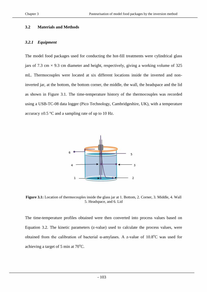
Chapter 3 Pasteurisation of model food packages by the inversion method
- 103
3.2 Materials and Methods
3.2.1 Equipment
The model food packages used for conducting the hot-fill treatments were cylindrical glass
jars of 7.3 cm × 9.3 cm diameter and height, respectively, giving a working volume of 325
mL. Thermocouples were located at six different locations inside the inverted and non-
inverted jar, at the bottom, the bottom corner, the middle, the wall, the headspace and the lid
as shown in Figure 3.1. The time-temperature history of the thermocouples was recorded
using a USB-TC-08 data logger (Pico Technology, Cambridgeshire, UK), with a temperature
accuracy ±0.5 °C and a sampling rate of up to 10 Hz.
Figure 3.1: Location of thermocouples inside the glass jar at 1. Bottom, 2. Corner, 3. Middle, 4. Wall
5. Headspace, and 6. Lid
The time-temperature profiles obtained were then converted into process values based on
Equation 3.2. The kinetic parameters (z-value) used to calculate the process values, were
obtained from the calibration of bacterial α-amylases. A z-value of 10.8oC was used for
achieving a target of 5 min at 70oC.
Chapter 3 Pasteurisation of model food packages by the inversion method
- 104
The fluids used in the hot-fill treatments were aqueous solutions of maize starch (Colflo 67,
Ingredion, Manchester, UK) of 3, 4 and 5% (w/w), and cream of tomato soup (Heinz Foods,
Wigan, UK), and their pasteurisation was conducted in a well-stirred water bath (Grant, UK).
For convenience, the model fluids will be referred to as A, B, C and T for the 3, 4, 5% of
starch solution, and tomato soup, respectively.
The samples were pre-gelatinised at the reference temperature of 80oC in the well-stirred for
approximately 80 min (the time needed for the model foods to reach the reference
temperature in the water bath) and were cooled down to ambient temperature. Samples of 2
mL of the pre-gelatinised fluids were then taken for rheological characterisation using a TA
AR1000 cone and plate rheometer (TA Instruments, Newcastle, Delaware, USA) equipped
with 0.06 m diameter 2o steel cone and plate geometry.
3.2.2 Inversion method
Duran® glass beakers of 1000 mL (Fisher Scientific UK Ltd) were filled with 700 mL of
each of the model foods and were immersed in the water bath, until the required filling
temperatures of 80oC was reached. A compact overhead stirrer (Fisher Scientific UK Ltd)
was used to continuously stir the liquid foods while being heated, to ensure thermal
uniformity. Once the desired fluid temperature was reached, two glass jars with their lids
screwed in were fully immersed into the water bath for approximately 5s, at the same
temperature as the fluid. Each of the two already heated glass jars was hot-filled with 290 mL
of the model food and sealed; the headspace of the container was kept lower than 10%,
volumetrically. After the two jars were sealed, one of them was inverted for 30 s, whilst the
other was at the upright position. After the 30 s, the inverted jar was brought back to the
upright position and was kept together with the non-inverted jar at ambient temperature for
approximately 10 min, as illustrated in Figure 3.2. At the end of the process, the lids of both
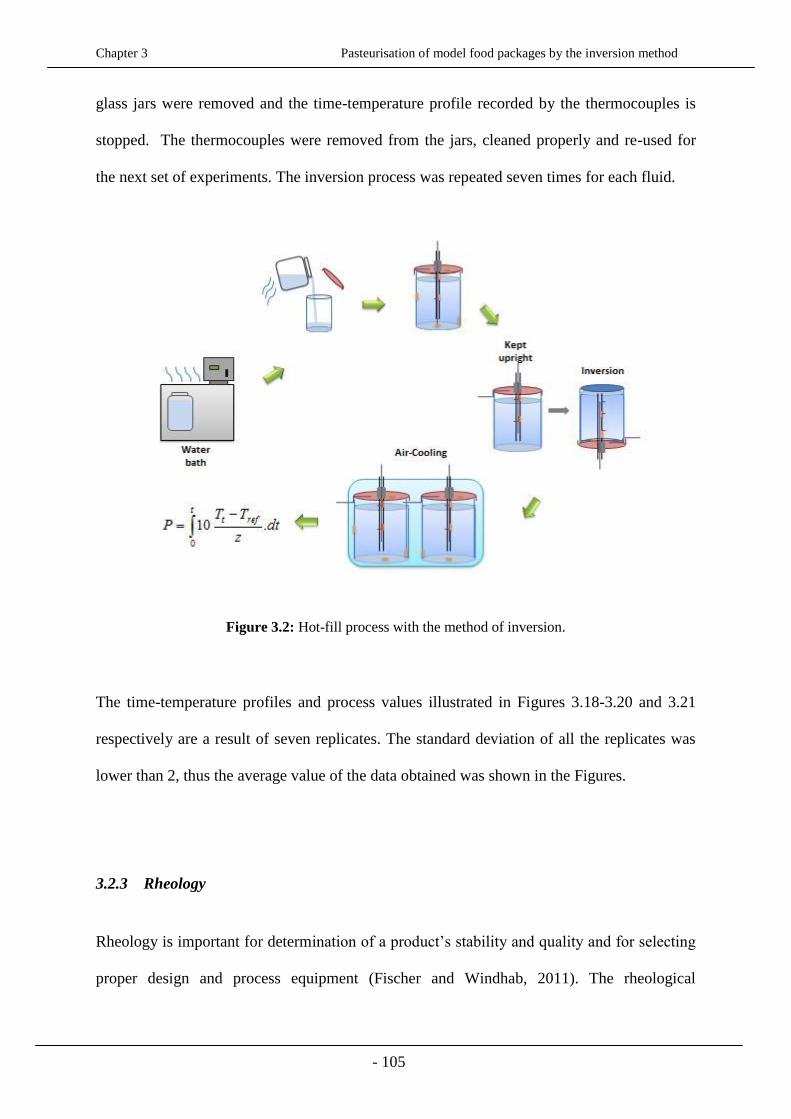
Chapter 3 Pasteurisation of model food packages by the inversion method
- 105
glass jars were removed and the time-temperature profile recorded by the thermocouples is
stopped. The thermocouples were removed from the jars, cleaned properly and re-used for
the next set of experiments. The inversion process was repeated seven times for each fluid.
Figure 3.2: Hot-fill process with the method of inversion.
The time-temperature profiles and process values illustrated in Figures 3.18-3.20 and 3.21
respectively are a result of seven replicates. The standard deviation of all the replicates was
lower than 2, thus the average value of the data obtained was shown in the Figures.
3.2.3 Rheology
Rheology is important for determination of a product’s stability and quality and for selecting
proper design and process equipment (Fischer and Windhab, 2011). The rheological

Chapter 3 Pasteurisation of model food packages by the inversion method
- 106
characteristics of food products can be determined by several methods, such as flow and
oscillatory measurements, which are performed to determine the flow behaviour and to
provide information about the viscoelastic properties of the materials tested, respectively.
The time-temperature profiles and process values illustrated in Figures 3.7-3.13 are a result of
five replicates. The standard deviation of all the replicates was lower than 2, thus the average
value of the data obtained was shown in the Figures.
3.2.3.1 Oscillatory measurements
Oscillation tests are used for determining the strength and stability of a material. They give a
clear indication of the behaviour of the sample, whether viscous or elastically dominated,
over a given frequency range. The nature of the tests is non-destructive, enabling
measurements to be made without incurring structural damage to the sample. Thus, the
dynamic rheological parameters are related to the sample's molecular structure. These tests
also provide a very sensitive means of studying the molecular motions that give rise to the
phenomenon like glass transition temperature (Winter H.H., 1997).
By subjecting a specimen to an oscillatory stress (σ) and determining the response, both the
elastic and viscous characteristics can be obtained. In the case of the cone-plate geometry, the
cone is forced into oscillatory shear with angular frequency ω and the sample is placed
between the plate and the cone, as illustrated in Figure 3.3.
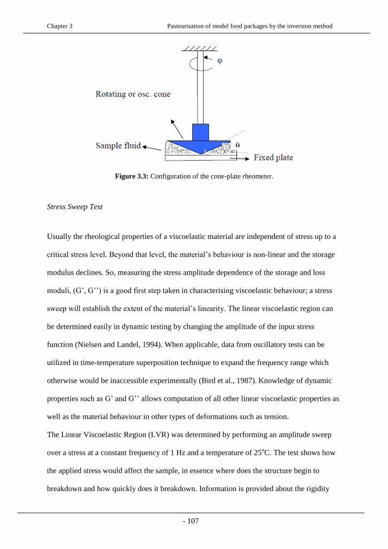
Chapter 3 Pasteurisation of model food packages by the inversion method
- 107
Figure 3.3: Configuration of the cone-plate rheometer.
Stress Sweep Test
Usually the rheological properties of a viscoelastic material are independent of stress up to a
critical stress level. Beyond that level, the material’s behaviour is non-linear and the storage
modulus declines. So, measuring the stress amplitude dependence of the storage and loss
moduli, (G’, G’’) is a good first step taken in characterising viscoelastic behaviour; a stress
sweep will establish the extent of the material’s linearity. The linear viscoelastic region can
be determined easily in dynamic testing by changing the amplitude of the input stress
function (Nielsen and Landel, 1994). When applicable, data from oscillatory tests can be
utilized in time-temperature superposition technique to expand the frequency range which
otherwise would be inaccessible experimentally (Bird et al., 1987). Knowledge of dynamic
properties such as G’ and G’’ allows computation of all other linear viscoelastic properties as
well as the material behaviour in other types of deformations such as tension.
The Linear Viscoelastic Region (LVR) was determined by performing an amplitude sweep
over a stress at a constant frequency of 1 Hz and a temperature of 25oC. The test shows how
the applied stress would affect the sample, in essence where does the structure begin to
breakdown and how quickly does it breakdown. Information is provided about the rigidity

Chapter 3 Pasteurisation of model food packages by the inversion method
- 108
and strength of products, such as delicately-structured fruit juices and thickened drinks
(Menard, 2008).
The behaviour of the fluids is expressed in terms of complex shear stress, and phase angle
against the oscillation stress applied (Figures 3.9 and 3.10). The complex modulus results
from the varying strain in the product and is the ratio of shear stress to shear strain (Figure
3.2), expressed as follows:
'''*minmax
minmax GiGG
(3.3)
Where: G´, G´´ and i are the dynamic storage modulus, the dynamic loss modulus and the
complex number 1 respectively. τmin / τmax (Pa) and γmin / γmax (s-1
) are the minimum and
maximum shear stress and shear rate, respectively.
Figure 3.4: Complex shear modulus
G* is the material’s overall resistance to shear deformation, and it is a good indicator of the
material’s flexibility or stiffness.
δ is the phase difference between the stress and strain, and if close to zero degrees means that
the material is highly elastic, whilst approaching the 90 degrees it is highly viscous and

Chapter 3 Pasteurisation of model food packages by the inversion method
- 109
demonstrates the greatest capability to dissipate energy. At 45 degrees, the material is
perfectly viscoelastic.
Figure 3.5: Viscoelasticity (Hesp, S. A. M.; Soleimani, 2009).
The LVR can be defined as the level where the complex modulus, drops to 90% of its
original value (Dealy et al., 2006). The viscoelastic behaviour of the fluids is characterised by
a critical oscillation value below which G´> G´´, indicating highly structured solutions and
above which G´ progressively declines until G´´ eventually exceeds it and the materials
behave in a fluid-like manner.
The length of the LVR is a measure of stability; all further oscillation analysis was being
performed within the LVR.
Frequency Sweep Test
After the fluid’s linear viscoelastic region has been defines by the stress sweep test, its
structure can be further characterised using a frequency sweep at a stress below the critical
stress σ. This provides more information about how time affects the sample and the effect of
colloidal forces and the interactions among particles. Materials usually become stronger (G’
γ (s-1)
τ (Pa)

Chapter 3 Pasteurisation of model food packages by the inversion method
- 110
increases) as the rate increases or the measurement time decreases. Cross over points for G’
and G’’ are commonly used as an indication of the sample’s relaxation time G’=G’’.
The materials’ response over a range of oscillation frequencies from 0.1-100 Hz, was
monitored at a constant temperature of 25oC and oscillation stress of 1 Pa, chosen from the
LVR region (determined from the stress sweep test). The frequency was plotted against the
complex modulus and phase angle δ, as shown in Figures 3.11 and 3.12, respectively.
Temperature Sweep Test
The temperature dependence of the steady and dynamic shear parameters was observed by
the conduction of a temperature sweep test. The samples were submitted to a shear rate of
10s-1
and the stress was maintained at 1 Pa for a frequency of 1 Hz. (Figure 3.13).
3.2.3.2 Flow measurements
Steady State Flow Test
The final test to be performed was that of steady state flow, for estimating the apparent
viscosities of the different solutions. The fixtures used were 50 mm diameter, 0.0399 rad
cone and plate, with the cone truncated at 0.048 mm from its vertex; the tests were run by
taking ten points per decade. Measurements at each shear rate were made in both the
clockwise and counter clockwise directions, with the shear applied for 20 s and then
measurements of the torque and normal force averaged over the next 30 s. Before loading
each sample, the cone and plate fixtures were installed and set to a nominal gap of 1 mm; the
gap was then zeroed using the Autozero capability of the AR1000 rheometer. The
temperature control chamber was then opened, and the upper fixture was raised

Chapter 3 Pasteurisation of model food packages by the inversion method
- 111
approximately 60 mm. A sample was then transferred to the lower plate fixture using a 3 mL
syringe. The upper cone fixture was lowered to a position of 0.040 mm and then the cone was
repositioned to the specified gap of 0.048 mm; this procedure was used in an effort to
compensate for the expansion of the sample and the fixtures when changing from room
temperature to the test temperature of 25 °C. The total time for a single test was
approximately 70 min, including the 10 min delay to ensure thermal steady state before
measurements were begun.
Approximately 2 mL of each sample was placed on the plate and a pre-shear phase was used
in order to ensure reproducible results; by pre-shearing the normal forced induced when the
geometry is closing reduces and the results become more reproducible. The samples are fully
hydrated and the previous history is destroyed enabling the measurement of the viscosity at a
defined point. Heymann et al., (2002), found that differences between storage (G´) and loss
moduli (G´´) were distinct when samples were pre-sheared; both moduli appeared to show
higher values after oscillatory pre-shear. For gel-like fluids, pre-shear is applied in order to
restore potential microstructural disruption in the tested fluid (Srinivasa et al., 1995). The
authors showed that G´ increases with increasing the pre-shear strain.
During the conditioning step, the samples were set at equilibration for 2 min and were pre-
sheared for 1 min at a shear stress of 100 s-1
. After the completion of the conditioning step,
the pre-gelatinised samples were subjected to a constant temperature of 25oC and a frequency
of 1 Hz, for a shear rate range of 0.01-1000 s-1
.
The data were best fitted by the Carreau rheological model (Figure 3.6), which describes a
wide range of fluids; it is mostly used to fit viscosity data for middle to high range of shear
rates. The model pieces together functions for Newtonian and shear-thinning (η<1) non-
Newtonian laws and it is expressed as follows:
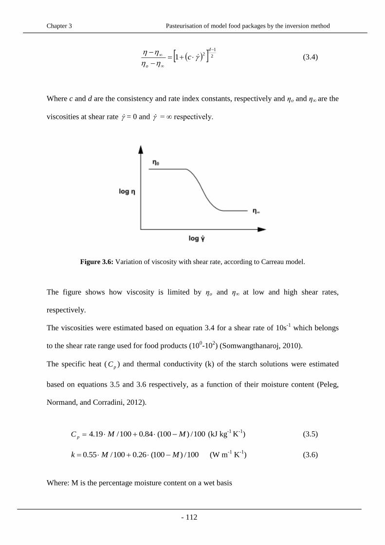
Chapter 3 Pasteurisation of model food packages by the inversion method
- 112
2
12
1
d
o
c
(3.4)
Where c and d are the consistency and rate index constants, respectively and ηο and η∞ are the
viscosities at shear rate = 0 and = ∞ respectively.
Figure 3.6: Variation of viscosity with shear rate, according to Carreau model.
The figure shows how viscosity is limited by ηο and η∞ at low and high shear rates,
respectively.
The viscosities were estimated based on equation 3.4 for a shear rate of 10s-1
which belongs
to the shear rate range used for food products (100-10
2) (Somwangthanaroj, 2010).
The specific heat (pC ) and thermal conductivity (k) of the starch solutions were estimated
based on equations 3.5 and 3.6 respectively, as a function of their moisture content (Peleg,
Normand, and Corradini, 2012).
pC 100/)100(84.0100/19.4 MM (kJ kg-1
K-1
) (3.5)
100/)100(26.0100/55.0 MMk (W m-1
K-1
) (3.6)
Where: M is the percentage moisture content on a wet basis
Chapter 3 Pasteurisation of model food packages by the inversion method
- 113
The specific heat of the cream of tomato soup was estimated based on equation 3.7 (Choi and
Okos, 1983), taking into account the composition of the solid components contained in the
soup.
afpwp XXcXXXC 908.0547.1928.1711.1180.4 (kJ kg-1
K-1
) (3.7)
Where: X is the mass fraction of each component and w, p, f, c and a, correspond
respectively to water, protein, fat, carbohydrates, and ash.
When data are not available, the thermal conductivity of biological materials such as the
cream of tomato soup can be estimated based on the water content. According to Anderson
(1950), the thermal conductivity can be estimates as follows;
)1( wsww XkXkk = 0.056 + 0.57 Xw (3.8)
Where: kw is the thermal conductivity of water and ks is that of the solid portion.
Finally, the densities of all fluids were measured/weighed on an Analytical Balance
(Sartorius ENTRIS224-1S, Massachusetts). The viscosities and thermal properties of the
fluids tested are presented in Table 3.2.
During the experiments, a solvent trap was used to minimise solvent loss.
All oscillatory and flow tests were repeated at least five times and the average was taken for
analysis.

Chapter 3 Pasteurisation of model food packages by the inversion method
- 114
3.2.4 Mathematical modelling
The steady state of free convection in a rectangular cavity filled with the model fluids used in
the experiments was studied by developing a mathematical model. COMSOL Multiphysics
4.3b (COMSOL Ltd, Cambridge, UK) was used to set up a convection model; the model
calculates the steady state velocity and temperature field with a predefined non-isothermal
flow interface which couples the heat transfer and fluid dynamics, provided in the Heat
Transfer Module.
The geometry and boundary conditions are shown in Figure 3.7. The cavity is consisted of
impermeable walls, i.e. with a zero flow boundary condition. To generate the buoyancy flow,
the left and right edges of the cavity were set at 20 and 30oC, respectively; the temperature
difference produces the density variation that drives the buoyant flow. The choice of the two
temperatures was random, since the parameter of interest was the temperature difference,
rather than the temperatures themselves. The goal of the developed model was to indicate
whether there is natural convection occurring in fluids of a specific viscosity or not. The
specific model was not aiming at mimicking the experimental conditions. Based on the
results obtained from the simulations, a new model was developed including the module of
natural convection, when the actual experiment was predicted.
The upper and lower boundaries are insulated i.e. zero heat flux boundary condition.
No-slip fluid boundary conditions were applied resulting in zero velocity at the wall, with
pressure remaining unidentified; the model contains information only about the pressure
gradient and it estimates the pressure field up to a constant (Incropera, 2006). Thus, in order
to define that constant and achieve convergence, the initial pressure field is set to be
consistent with the volume force. The initial pressure field must be also consistent with the
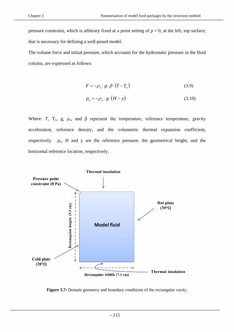
Chapter 3 Pasteurisation of model food packages by the inversion method
- 115
pressure constraint, which is arbitrary fixed at a point setting of p = 0, at the left, top surface;
that is necessary for defining a well-posed model.
The volume force and initial pressure, which accounts for the hydrostatic pressure in the fluid
column, are expressed as follows:
oo TTgF (3.9)
yHgp oo (3.10)
Where: T, To, g, ρo, and β represent the temperature, reference temperature, gravity
acceleration, reference density, and the volumetric thermal expansion coefficient,
respectively. po, H and y are the reference pressure, the geometrical height, and the
horizontal reference location, respectively.
Figure 3.7: Domain geometry and boundary conditions of the rectangular cavity.
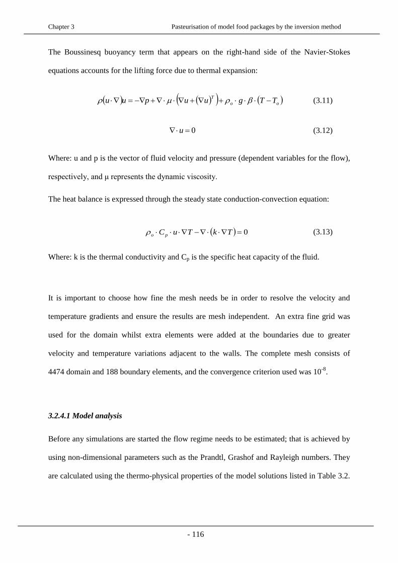
Chapter 3 Pasteurisation of model food packages by the inversion method
- 116
The Boussinesq buoyancy term that appears on the right-hand side of the Navier-Stokes
equations accounts for the lifting force due to thermal expansion:
oo
TTTguupuu (3.11)
0 u (3.12)
Where: u and p is the vector of fluid velocity and pressure (dependent variables for the flow),
respectively, and μ represents the dynamic viscosity.
The heat balance is expressed through the steady state conduction-convection equation:
0 TkTuC po (3.13)
Where: k is the thermal conductivity and Cp is the specific heat capacity of the fluid.
It is important to choose how fine the mesh needs be in order to resolve the velocity and
temperature gradients and ensure the results are mesh independent. An extra fine grid was
used for the domain whilst extra elements were added at the boundaries due to greater
velocity and temperature variations adjacent to the walls. The complete mesh consists of
4474 domain and 188 boundary elements, and the convergence criterion used was 10-8
.
3.2.4.1 Model analysis
Before any simulations are started the flow regime needs to be estimated; that is achieved by
using non-dimensional parameters such as the Prandtl, Grashof and Rayleigh numbers. They
are calculated using the thermo-physical properties of the model solutions listed in Table 3.2.

Chapter 3 Pasteurisation of model food packages by the inversion method
- 117
The thermo-physical properties are given at 25oC which is in the range of the temperatures
used in the model.
In fluid mechanics working with non-dimensional numbers is a common and convenient way
to reduce the number of dependent and independent parameters. The non-dimensional
numbers used in the current work are the following:
The Prandtl number, Pr, is defined as the ratio of fluid viscosity to thermal diffusivity and it
is expressed by:
k
c p
Pr (3.14)
Where: pC
k
(3.15)
α = thermal diffusivity (m2 s
-1), Cp = specific heat (J kg
-1 K
-1), ν = kinematic viscosity (m
2 s
-
1)=μ/ρ (dynamic viscosity/density).μ= dynamic viscosity (Pa s), and k = thermal conductivity
of the fluid (W m-1
K-1
).
The Reynolds number, Re, is defined as the ratio of inertial forces to viscous forces and it is
used to predict the flow regime of the fluids; it is expressed by the following expression:
LU Re (3.16)
Where: U is the typical velocity (m s-1) and L the typical length (m)
When a viscous fluid flows along a fixed impermeable wall, the velocity at any point on the
wall will be zero due to the no-slip condition. The extent to which the boundary layer at the
wall develops along the length of the wall depends upon the value Re, and hence on the
viscosity.
Chapter 3 Pasteurisation of model food packages by the inversion method
- 118
Figure 3.8: No-slip condition and boundary layer development.
Where: u and ν are the velocities (m s-1
) at the wall along x and y, respectively.
The viscosity of the model fluids used in the current work is high and the flow is in the
laminar/transitional regimes. Hence the boundary layers are important; the fluid velocity
within the boundary layers changes rapidly from zero to its main-stream value possibly
implying a steep gradient of shear stress (Burr, 2010). The majority of the resistance to heat
transfer takes place within the boundary layer, whilst the pressure distribution throughout it
remains constant.
The velocity boundary layer thickness can be defined as the distance from the wall at which
the viscous flow velocity is 99% of the free stream velocity and can be obtained in terms of
the Reynolds number, using the following equation:
Re
LM (3.17)
The thermal boundary layer, δT, which similarly to the velocity boundary layer is the distance
from the wall, at which the temperature is 99% of the temperature found at the region where
the fluid stabilises, can be defined by the Prandtl number.
For Pr>>1, the ratio of the two thicknesses is governed by the following equation:
Chapter 3 Pasteurisation of model food packages by the inversion method
- 119
PrT
(3.18)
The Grashof number, Gr, is defined as the ratio of buoyancy to viscous forces and it is
described as follows:
2
32 )(
LTTgGr s
(3.19)
Where: g = acceleration due to Earth's gravity (m s-2
), β = volumetric thermal expansion
coefficient (K-1
), Ts = surface temperature (K), T∞ = bulk temperature (K), L = the distance
between the highest (bulk) and lowest temperature (headspace) along the cylinder (m).
The volumetric thermal expansion coefficient was estimated based on the Boussinesq
approximation, as expressed by Adrian, (1993):
T
1 (3.20)
Where: (kg m-3
) and TTT (oC) between the bulk of the fluid and the
headspace.
The Grashof number can also be expressed as the velocity ratio:
2
2
0
/ L
UGr
(3.21)
Where Uo = typical velocity due to buoyancy forces, defined by:
Chapter 3 Pasteurisation of model food packages by the inversion method
- 120
LTgU 0 (3.22)
The critical Grashof number value that indicates the transition between laminar (larger
buoyancy forces) and turbulent (larger viscous forces) flow is 109.
The Rayleigh number, Ra, is another indicator of free convection, and is defined as:
LLL GrLTg
Ra Pr32
(3.23)
Like the Grashof number, a critical Rayleigh value indicates the transition between laminar
and turbulent flow, which is about 109.
The viscous forces limit the buoyancy effects and may result in an overestimated typical
velocity, obtained by Uo. Thus, another approach, where the thermal diffusivity and viscosity
of the fluids are included should be more accurate in estimating the typical velocity. U1 is
used instead and is defined as follows:
RaL
U
1 or Pr
1oU
U (3.24)
The Grashof and Rayleigh numbers need first to be calculated in order to characterise the
flow regime. If they are significantly below the critical order of 109, the regime is laminar and
in that case Equation 3.21 or Equation 3.24 provide estimates of the typical velocity U that
can be used to validate the model after performing the simulation.
Chapter 3 Pasteurisation of model food packages by the inversion method
- 121
3.3 Results and Discussion
3.3.1 Rheology
The model fluids’ (A, B, C, and T) response to increasing stress was monitored by the stress
sweep test, see Figure 3.9; the samples were subjected to small amplitude oscillatory shear.
Initially the applied stress is low and the material structure is preserved, but as the test
progresses, the increased stresses cause disruption, which is demonstrated by a decrease in
elasticity, with a phase angle (δ) rise (Figure 3.10), and a decrease in rigidity, which is
expressed by the complex modulus (G*).
The LVR of the solutions was defined for a constant frequency of 1 Hz and a temperature of
25oC, and it lies in the range of 0.01-1 Pa, 0.01-1.5 Pa, 0.01-2 Pa, and 0.01-6 Pa for solutions
A, B, C and T, respectively. The longer the LVR, the more stable the system is, expecting the
solution of 5% starch (C) to show higher resistance in amplitudes of stress, strain, frequency
or temperature when those are applied.
The value of oscillation stress chosen for subsequent testing was 1 Pa, which is below the
critical oscillation stress for all fluids (1, 1.5, 2 and 6 Pa for A, B, T and C, respectively) and
consequently lies within their LVR region.
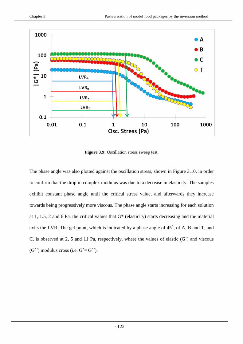
Chapter 3 Pasteurisation of model food packages by the inversion method
- 122
Figure 3.9: Oscillation stress sweep test.
The phase angle was also plotted against the oscillation stress, shown in Figure 3.10, in order
to confirm that the drop in complex modulus was due to a decrease in elasticity. The samples
exhibit constant phase angle until the critical stress value, and afterwards they increase
towards being progressively more viscous. The phase angle starts increasing for each solution
at 1, 1.5, 2 and 6 Pa, the critical values that G* (elasticity) starts decreasing and the material
exits the LVR. The gel point, which is indicated by a phase angle of 45o, of A, B and T, and
C, is observed at 2, 5 and 11 Pa, respectively, where the values of elastic (G´) and viscous
(G´´) modulus cross (i.e. G´= G´´).
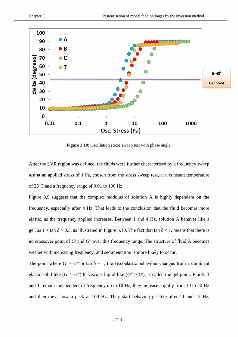
Chapter 3 Pasteurisation of model food packages by the inversion method
- 123
Figure 3.10: Oscillation stress sweep test with phase angle.
After the LVR region was defined, the fluids were further characterised by a frequency sweep
test at an applied stress of 1 Pa, chosen from the stress sweep test, at a constant temperature
of 25oC and a frequency range of 0.01 to 100 Hz.
Figure 3.9 suggests that the complex modulus of solution A is highly dependent on the
frequency, especially after 4 Hz. That leads to the conclusion that the fluid becomes more
elastic, as the frequency applied increases. Between 1 and 4 Hz, solution A behaves like a
gel, as 1 > tan δ > 0.5, as illustrated in Figure 3.10. The fact that tan δ < 1, means that there is
no crossover point of G′ and G″ over this frequency range. The structure of fluid A becomes
weaker with increasing frequency, and sedimentation is more likely to occur.
The point where G′ = G″ or tan δ = 1, the viscoelastic behaviour changes from a dominant
elastic solid-like (G′ > G″) to viscous liquid-like (G″ > G′), is called the gel point. Fluids B
and T remain independent of frequency up to 10 Hz, they increase slightly from 10 to 40 Hz
and then they show a peak at 100 Hz. They start behaving gel-like after 11 and 12 Hz,
δ=45o
Gel point

Chapter 3 Pasteurisation of model food packages by the inversion method
- 124
respectively (1 > tan δ > 0.5), and there is no cross point of the elastic and viscous modulus at
any point throughout the test (tan δ < 1).
When 1 > tan δ > 0.5, the material tested behaves gel like (Augusto, 2012).
Solution C is the most stable, as expected from the stress sweep test (the longest LVR). G* is
independent of frequency throughout the test, and tan δ range is the lowest of all fluids (tan δ
< 0.5); it is the most elastic fluid. Fluids B, T, and C have strongly associated particles, and
sedimentation is unlikely to occur. The storage modulus (G´) is higher than the loss modulus
(G″), for all fluids, along the whole frequency range studied, which indicates that the fluids
have dominant elastic properties rather than the viscous ones. Thus, the product can be
classified as weak gels (Rao, 2005). This kind of behaviour is mostly observed in suspensions
with network-like structure, such as fruit products, tomato products and fruit purees (Massa et
al., 2010). The frequency chosen to be used for subsequent tests was 1 Hz, a value at which
all the fluids are frequency independent and more stable.
Figure 3.11: Frequency sweep test at 25oC and oscillation stress 1 Pa.

Chapter 3 Pasteurisation of model food packages by the inversion method
- 125
Figure 3.12: Frequency sweep test at 25oC and oscillation stress 1 Pa with phase angle.
For the temperature sweep test, the model foods were prepared at room temperature and were
heated up on the Peltier plate of the rheometer for 40 min at a temperature range between 25
and 85oC, at a rate of 5
oC min
-1. The stress and frequency were maintained at 1 Pa and 1 Hz,
respectively. The temperature was plotted against the complex modulus, Figure 3.13, and the
tangent phase angle, Figure 3.14. As the temperature increases, the complex modulus (G*)
remains constant until the fluids start gelatinising and reach the maximum viscosity and
volume at approximately 85oC.
Starch granules, when heated in excess water (i.e., water-starch ratios > 1.5:1) lose their
molecular order in an irreversible way (gelatinisation), resulting in an increased granule
hydration, swelling and possibly the leaching of soluble components, such as amylose. The
hydrated molecules progressively vibrate, inducing hydrogen bonds disruption, which
eventually leads to the plasticisation of the starch molecules within granules. If the starch
concentration present is sufficiently high (typically 2–7%), the granules swell and start to
tan (δ)=0.5
Gel point
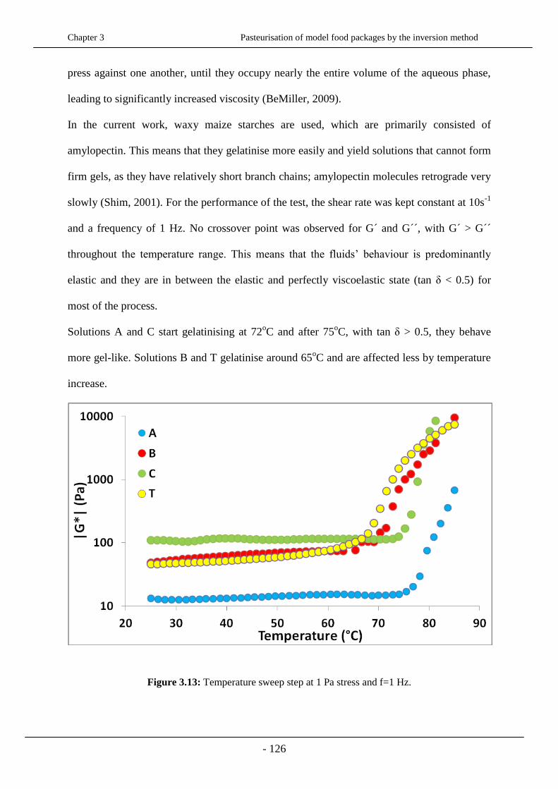
Chapter 3 Pasteurisation of model food packages by the inversion method
- 126
press against one another, until they occupy nearly the entire volume of the aqueous phase,
leading to significantly increased viscosity (BeMiller, 2009).
In the current work, waxy maize starches are used, which are primarily consisted of
amylopectin. This means that they gelatinise more easily and yield solutions that cannot form
firm gels, as they have relatively short branch chains; amylopectin molecules retrograde very
slowly (Shim, 2001). For the performance of the test, the shear rate was kept constant at 10s-1
and a frequency of 1 Hz. No crossover point was observed for G´ and G´´, with G´ > G´´
throughout the temperature range. This means that the fluids’ behaviour is predominantly
elastic and they are in between the elastic and perfectly viscoelastic state (tan δ < 0.5) for
most of the process.
Solutions A and C start gelatinising at 72oC and after 75
oC, with tan δ > 0.5, they behave
more gel-like. Solutions B and T gelatinise around 65oC and are affected less by temperature
increase.
Figure 3.13: Temperature sweep step at 1 Pa stress and f=1 Hz.
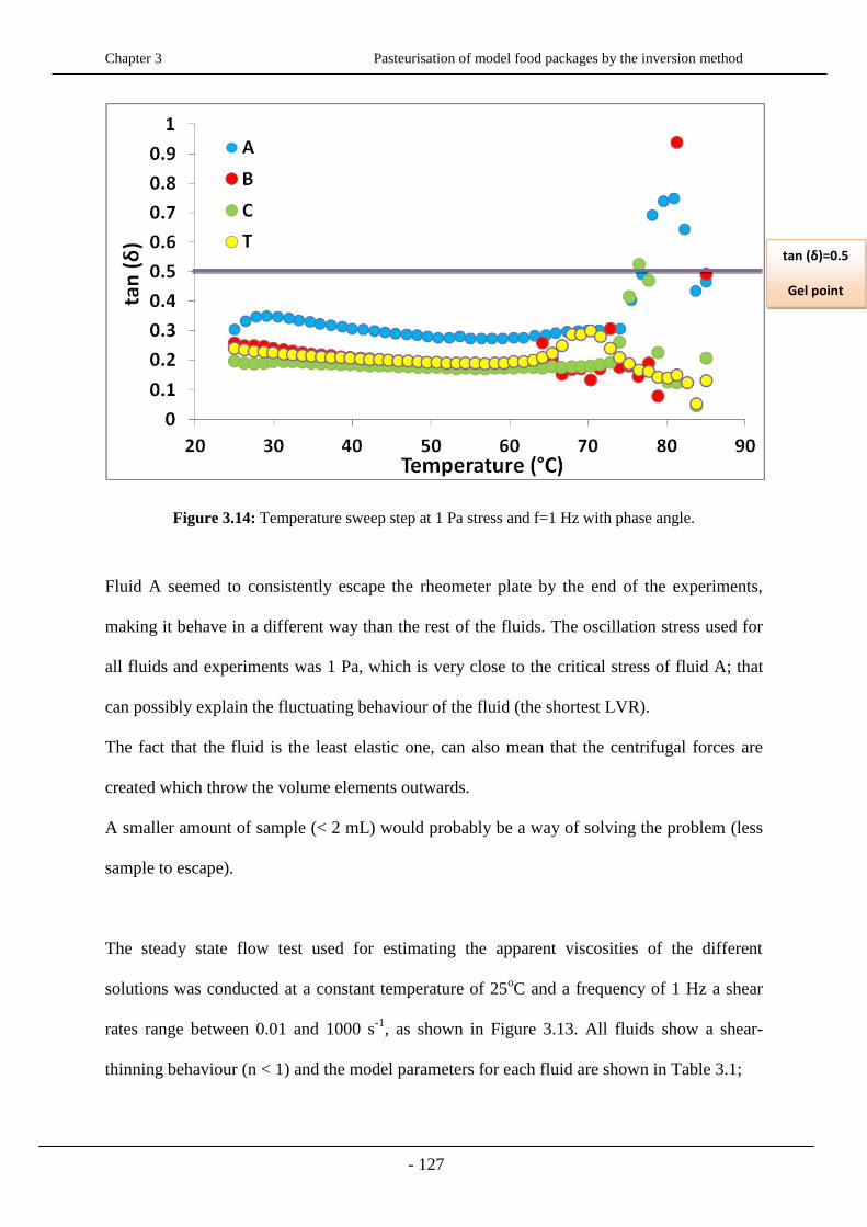
Chapter 3 Pasteurisation of model food packages by the inversion method
- 127
Figure 3.14: Temperature sweep step at 1 Pa stress and f=1 Hz with phase angle.
Fluid A seemed to consistently escape the rheometer plate by the end of the experiments,
making it behave in a different way than the rest of the fluids. The oscillation stress used for
all fluids and experiments was 1 Pa, which is very close to the critical stress of fluid A; that
can possibly explain the fluctuating behaviour of the fluid (the shortest LVR).
The fact that the fluid is the least elastic one, can also mean that the centrifugal forces are
created which throw the volume elements outwards.
A smaller amount of sample (< 2 mL) would probably be a way of solving the problem (less
sample to escape).
The steady state flow test used for estimating the apparent viscosities of the different
solutions was conducted at a constant temperature of 25oC and a frequency of 1 Hz a shear
rates range between 0.01 and 1000 s-1
, as shown in Figure 3.13. All fluids show a shear-
thinning behaviour (n < 1) and the model parameters for each fluid are shown in Table 3.1;
tan (δ)=0.5
Gel point
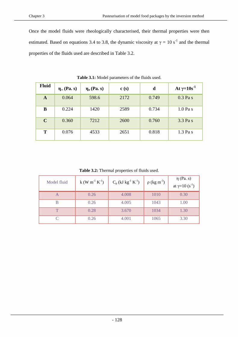
Chapter 3 Pasteurisation of model food packages by the inversion method
- 128
Once the model fluids were rheologically characterised, their thermal properties were then
estimated. Based on equations 3.4 to 3.8, the dynamic viscosity at γ = 10 s-1
and the thermal
properties of the fluids used are described in Table 3.2.
Table 3.1: Model parameters of the fluids used.
Fluid η∞ (Pa. s) ηο (Pa. s) c (s) d At γ=10s
-1
A 0.064 598.6 2172 0.749 0.3 Pa s
B 0.224 1420 2589 0.734 1.0 Pa s
C 0.360 7212 2600 0.760 3.3 Pa s
T 0.076 4533 2651 0.818 1.3 Pa s
Table 3.2: Thermal properties of fluids used.
Model fluid k (W m-1
K-1
) Cp (kJ kg-1
K-1
) ρ (kg m-3
) η (Pa. s)
at γ=10 (s-1
)
A 0.26 4.008 1010 0.30
B 0.26 4.005 1043 1.00
T 0.28 3.670 1034 1.30
C 0.26 4.001 1065 3.30
Chapter 3 Pasteurisation of model food packages by the inversion method
- 129
Figure 3.15: Steady state flow at γ = 10 s-1
and T = 25oC
3.3.2 Numerical simulations
As indicated in §3.2, the flow regime of the fluids in a rectangular cavity consisted of a cold
and hot wall and insulated bottom and top surface, was examined by calculating the
dimensionless Grashof, Rayleigh, Prandtl and Reynolds numbers. From the results obtained
the Ra number for all four model fluids belongs to the range 104
< RaL <109 and thus laminar
regime is expected; according to LeFevre, (1956), the above range indicates the occurrence of
laminar natural convection. Heat transfer is conduction dominated until a critical Ra number
is reached; according to Heslot et al. (1987) and Henkes (1990), that critical Ra number
equals to 1708. By increasing the temperature difference, the Ra number is increased and the
flow pattern changes.
Experiments conducted from the above authors in cylindrical geometries and square cavities
heated from the vertical walls and insulated from the horizontal ones, support that for 6×10³
<

Chapter 3 Pasteurisation of model food packages by the inversion method
- 130
Ra <1.5×10⁵ laminar convection occurs, whilst from 1.5×10
5 to 2.5×10
5, the flow becomes
chaotic; turbulence appears at a Ra ≥ 106.
According to the values estimated in the current work and based on the above findings,
steady laminar convection is expected by fluids T and C, the most viscous ones, whilst a
more chaotic behaviour is expected by fluid B and especially by fluid A. The typical velocity
(U1) was estimated to be in the range of 0.3 to 1 mm s-1
, with the lowest and highest value
corresponding to fluids C and A, respectively; the least viscous solution, fluid A, appears to
reach a velocity up to three times higher than the rest of the fluids, making the occurrence of
convection more possible and/or evident as compared to the rest of the fluids.
The dimensionless parameters and typical velocities for each model fluid are presented in
Table 3.3.
Table 3.3: Dimensionless numbers and velocity used in heat treatment.
Fluid Gr Pr Ra Re U1 (mm s-1
)
A 200 3.7×10³ 7.0x10
5 0.2 1
B 20 1.3x10⁴ 2.0x10
5 0.04 0.5
T 10 1.6x10⁴ 1.5x10
5 0.03 0.4
C 2 4.0x10⁴ 7.0x10
4 0.01 0.3
The simulated data were presented in terms of velocity magnitude and temperature isotherms
for a temperature difference of 10oC between the cold and hot vertical wall, for all the model
fluids as illustrated in Figures 3.16 and 3.17, respectively.
The highest velocity values for all fluids appear to be located at the lateral boundaries where
the highest variations of temperature occur, indicating that the natural convection occurs from
the boundaries. The maximum velocity values for fluid A, B, T and C is 1.3, 0.4, 0.4 and 0.1

Chapter 3 Pasteurisation of model food packages by the inversion method
- 131
mm s-1
, respectively; the velocities are of similar order of magnitude to the estimated typical
velocities U1 of the order 1, 0.5, 0.4 and 0.3 mm s-1
shown in Table 3.3.
A) B)
T) C)
Figure 3.16: Velocity magnitude (mm/s) of A, B, T and C fluids at ΔT = 10oC.
Figure 3.17 shows the temperature field (surface) and velocity field (arrows) of the 2D
model. The fluid flow seems to follow the boundaries, with the highest variations observed at
the boundaries, especially at lateral walls, which are responsible for the free convection; the
temperature and velocity variations are smoother at the core of the fluid, with the most
viscous one (fluid C) showing a more distinct separation of the cold and hot zone; that is due
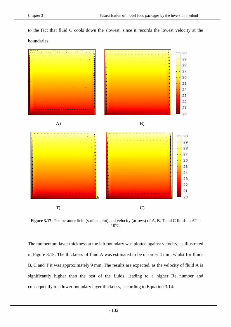
Chapter 3 Pasteurisation of model food packages by the inversion method
- 132
to the fact that fluid C cools down the slowest, since it records the lowest velocity at the
boundaries.
A) B)
6
T) C)
Figure 3.17: Temperature field (surface plot) and velocity (arrows) of A, B, T and C fluids at ΔT =
10oC.
The momentum layer thickness at the left boundary was plotted against velocity, as illustrated
in Figure 3.18. The thickness of fluid A was estimated to be of order 4 mm, whilst for fluids
B, C and T it was approximately 9 mm. The results are expected, as the velocity of fluid A is
significantly higher than the rest of the fluids, leading to a higher Re number and
consequently to a lower boundary layer thickness, according to Equation 3.14.
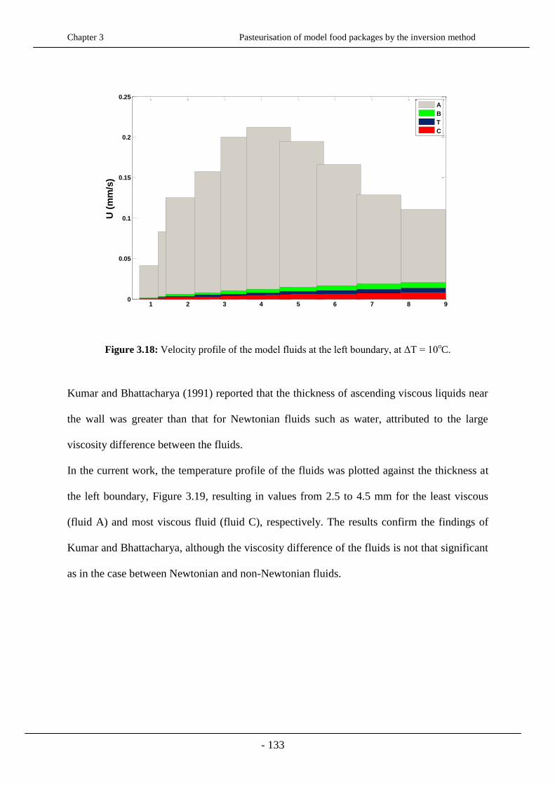
Chapter 3 Pasteurisation of model food packages by the inversion method
- 133
1 2 3 4 5 6 7 8 9
x 10-3
0
0.05
0.1
0.15
0.2
0.25
Arc length
U (
mm
/s)
A
B
T
C
Figure 3.18: Velocity profile of the model fluids at the left boundary, at ΔT = 10oC.
Kumar and Bhattacharya (1991) reported that the thickness of ascending viscous liquids near
the wall was greater than that for Newtonian fluids such as water, attributed to the large
viscosity difference between the fluids.
In the current work, the temperature profile of the fluids was plotted against the thickness at
the left boundary, Figure 3.19, resulting in values from 2.5 to 4.5 mm for the least viscous
(fluid A) and most viscous fluid (fluid C), respectively. The results confirm the findings of
Kumar and Bhattacharya, although the viscosity difference of the fluids is not that significant
as in the case between Newtonian and non-Newtonian fluids.
Distance from wall
(mm)
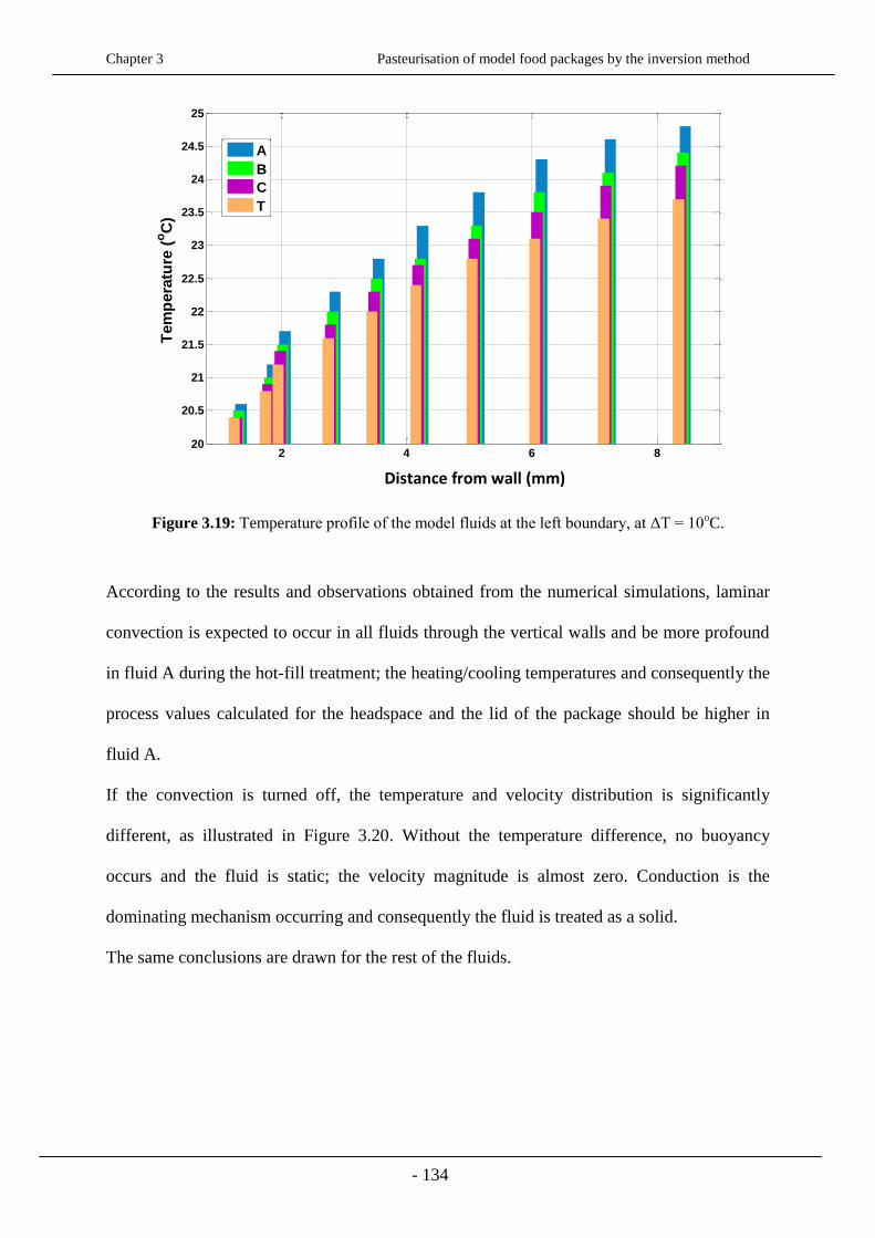
Chapter 3 Pasteurisation of model food packages by the inversion method
- 134
2 4 6 8
x 10-3
20
20.5
21
21.5
22
22.5
23
23.5
24
24.5
25
Arc length
Tem
pera
ture
(oC
)
A
B
C
T
Figure 3.19: Temperature profile of the model fluids at the left boundary, at ΔT = 10oC.
According to the results and observations obtained from the numerical simulations, laminar
convection is expected to occur in all fluids through the vertical walls and be more profound
in fluid A during the hot-fill treatment; the heating/cooling temperatures and consequently the
process values calculated for the headspace and the lid of the package should be higher in
fluid A.
If the convection is turned off, the temperature and velocity distribution is significantly
different, as illustrated in Figure 3.20. Without the temperature difference, no buoyancy
occurs and the fluid is static; the velocity magnitude is almost zero. Conduction is the
dominating mechanism occurring and consequently the fluid is treated as a solid.
The same conclusions are drawn for the rest of the fluids.
Distance from wall (mm)

Chapter 3 Pasteurisation of model food packages by the inversion method
- 135
Figure 3.20: Temperature field and velocity magnitude (mm/s) of fluid A, with ΔT = 0oC, between
the two walls (Figure 3.5).
3.3.3 Effectiveness of the inversion method
The recorded time-temperature history of the model fluids at the six different locations inside
the inverted and non-inverted jars, are illustrated in Figures 3.21-3.23.
The temperature at the bottom and corner of the non-inverted jars is recorded to be the lowest
for fluid A and the highest for fluid C, which is expected since the least viscous fluid cools
down faster. That is confirmed by the estimated higher velocity and consequently higher heat
transfer within fluid A, shown in Table 3.3. As far as the inverted jars are concerned, an
average temperature drop of 1, 2, 2 and 3oC is recorded for fluids A, B, T and C, respectively
since the two locations are exposed to air for 30 seconds; the highest drop, 3oC is observed
for fluid C which exhibits the lowest heating rate.
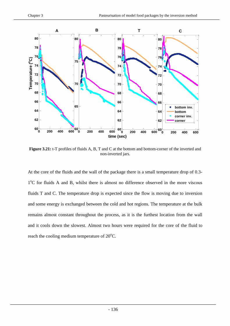
Chapter 3 Pasteurisation of model food packages by the inversion method
- 136
0 200 400 60060
62
64
66
68
70
72
74
76
78
80
Tem
pera
ture
(oC
)A
0 200 400 60060
65
70
75
80
time (sec)
B
0 200 400 60060
62
64
66
68
70
72
74
76
78
80
C
0 200 400 60060
62
64
66
68
70
72
74
76
78
80
T
bottom inv.
bottom
corner inv.
corner
Figure 3.21: t-T profiles of fluids A, B, T and C at the bottom and bottom-corner of the inverted and
non-inverted jars.
At the core of the fluids and the wall of the package there is a small temperature drop of 0.3-
1oC for fluids A and B, whilst there is almost no difference observed in the more viscous
fluids T and C. The temperature drop is expected since the flow is moving due to inversion
and some energy is exchanged between the cold and hot regions. The temperature at the bulk
remains almost constant throughout the process, as it is the furthest location from the wall
and it cools down the slowest. Almost two hours were required for the core of the fluid to
reach the cooling medium temperature of 20oC.
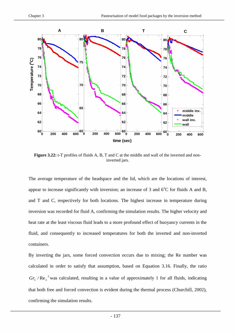
Chapter 3 Pasteurisation of model food packages by the inversion method
- 137
0 200 400 60060
62
64
66
68
70
72
74
76
78
80
time (sec)
Tem
pera
ture
(oC
)A
0 200 400 60060
62
64
66
68
70
72
74
76
78
80
C
0 200 400 60060
62
64
66
68
70
72
74
76
78
80
T
0 200 400 60060
65
70
75
80
B
middle inv.
middle
wall inv.
wall
Figure 3.22: t-T profiles of fluids A, B, T and C at the middle and wall of the inverted and non-
inverted jars.
The average temperature of the headspace and the lid, which are the locations of interest,
appear to increase significantly with inversion; an increase of 3 and 6oC for fluids A and B,
and T and C, respectively for both locations. The highest increase in temperature during
inversion was recorded for fluid A, confirming the simulation results. The higher velocity and
heat rate at the least viscous fluid leads to a more profound effect of buoyancy currents in the
fluid, and consequently to increased temperatures for both the inverted and non-inverted
containers.
By inverting the jars, some forced convection occurs due to mixing; the Re number was
calculated in order to satisfy that assumption, based on Equation 3.16. Finally, the ratio
2Re/ LLGr was calculated, resulting in a value of approximately 1 for all fluids, indicating
that both free and forced convection is evident during the thermal process (Churchill, 2002),
confirming the simulation results.
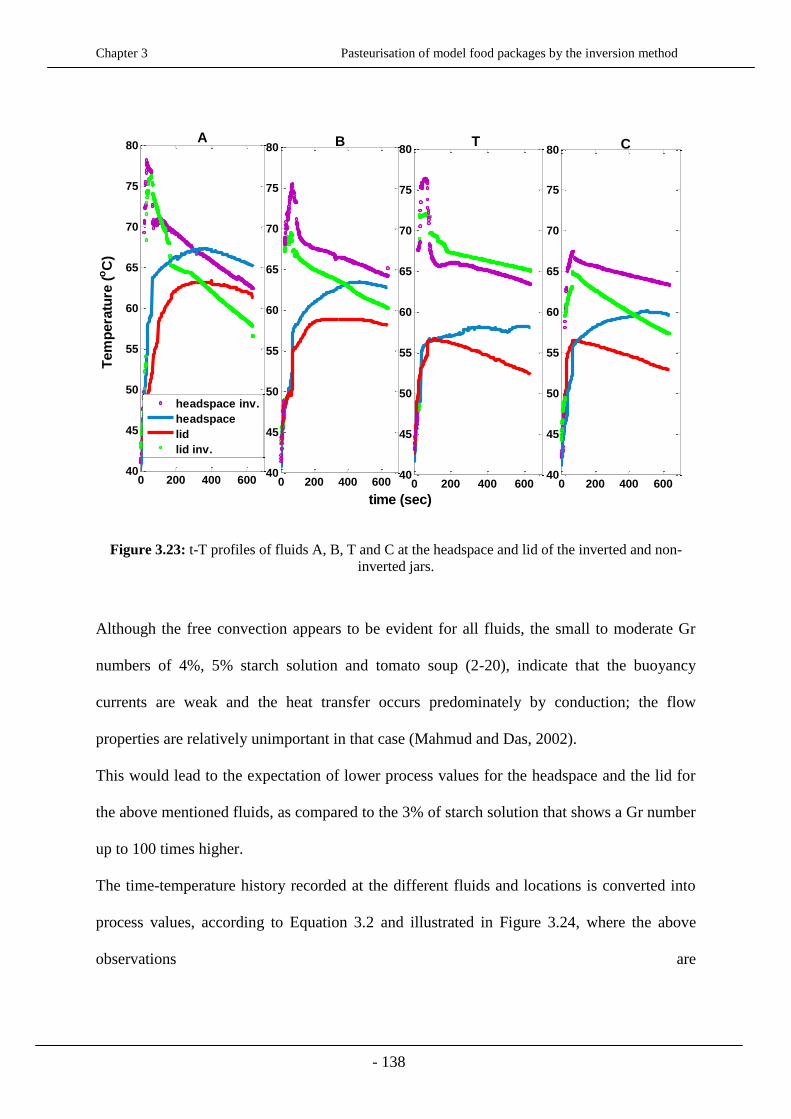
Chapter 3 Pasteurisation of model food packages by the inversion method
- 138
0 200 400 60040
45
50
55
60
65
70
75
80
time (sec)
Tem
pera
ture
(oC
)
A
0 200 400 60040
45
50
55
60
65
70
75
80 B
0 200 400 60040
45
50
55
60
65
70
75
80T
0 200 400 60040
45
50
55
60
65
70
75
80 C
headspace inv.
headspace
lid
lid inv.
Figure 3.23: t-T profiles of fluids A, B, T and C at the headspace and lid of the inverted and non-
inverted jars.
Although the free convection appears to be evident for all fluids, the small to moderate Gr
numbers of 4%, 5% starch solution and tomato soup (2-20), indicate that the buoyancy
currents are weak and the heat transfer occurs predominately by conduction; the flow
properties are relatively unimportant in that case (Mahmud and Das, 2002).
This would lead to the expectation of lower process values for the headspace and the lid for
the above mentioned fluids, as compared to the 3% of starch solution that shows a Gr number
up to 100 times higher.
The time-temperature history recorded at the different fluids and locations is converted into
process values, according to Equation 3.2 and illustrated in Figure 3.24, where the above
observations are

Chapter 3 Pasteurisation of model food packages by the inversion method
- 139
refle
Figure 3.24: Calculated process values for fluids A, B, T and C at a Tref of 70oC and a z-value of
10.8oC.
According to Figure 3.24, the target process is achieved by all locations for fluids A and T,
but not achieved for fluid B at the lid and fluid C at neither the headspace nor the lid.
The model fluids follow the same trend with the time-temperature profiles, with the process
values increasing with viscosity at the bottom, corner, middle and wall, but decreasing at the
headspace and the lid. An important point to be made from the above Figure is that the
bottom and corner of the jars do not get significantly colder with inversion; it appears that the
length of inversion time is sufficient to heat up the headspace and the lid but not long enough
to significantly cool down the bottom and the corner.
The target process line drawn shows by how much the chosen inversion time and filling
temperature combination, exceeds or misses the target set. Based on the above figure,
Target: 5 min

Chapter 3 Pasteurisation of model food packages by the inversion method
- 140
equivalent inversion time- filling temperature combinations were suggested for achieving a
process 5 min for the headspace and the lid illustrated in Figures 3.25 and 3.26, respectively.
6-9 30 60 12078
80
82
84
86
88
Inversion time (sec)
Fil
lin
g T
em
pe
ratu
re (
oC
)
A B T C
Figure 3.25: t-T combinations for achieving the target process at the headspace
6-9 30 60 12078
80
82
84
86
88
90
92
Inversion time (sec)
Fil
lin
g T
em
pe
ratu
re (
oC
)
A B T C
Figure 3.26: t-T combinations for achieving the target process at the lid.
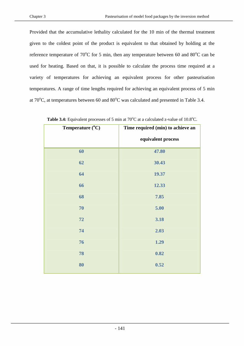
Chapter 3 Pasteurisation of model food packages by the inversion method
- 141
Provided that the accumulative lethality calculated for the 10 min of the thermal treatment
given to the coldest point of the product is equivalent to that obtained by holding at the
reference temperature of 70oC for 5 min, then any temperature between 60 and 80
oC can be
used for heating. Based on that, it is possible to calculate the process time required at a
variety of temperatures for achieving an equivalent process for other pasteurisation
temperatures. A range of time lengths required for achieving an equivalent process of 5 min
at 70oC, at temperatures between 60 and 80
oC was calculated and presented in Table 3.4.
Table 3.4: Equivalent processes of 5 min at 70oC at a calculated z-value of 10.8
oC.
Temperature (oC) Time required (min) to achieve an
equivalent process
60
62
64
66
68
70
72
74
76
78
80
47.80
30.43
19.37
12.33
7.85
5.00
3.18
2.03
1.29
0.82
0.52
Chapter 3 Pasteurisation of model food packages by the inversion method
- 142
3.4 Conclusions
The effectiveness of the inversion method as a treatment for the headspace and the lid, for
hot-filled model foods, tomato soup, and starch solutions of 3, 4, and 5% (w/w), was
investigated targeting a process of 5 min at 70oC.
The jars were hot-filled at a temperature of 80oC, sealed, inverted for 30 sec, brought back to
the upright position and cooled at room temperature for approximately 10 min. The inversion
time and filing temperature combination chosen appeared to be sufficient for achieving the
goal set, for fluids A and B at all locations, whilst it was not sufficient for the headspace and
the headspace and nor the lid of fluids T and C, respectively. The inverted jars showed
significantly higher process values for the headspace and the lid with the filling temperature
being the most important parameter. Based on the time temperature profiles used during the
thermal treatment, more inversion time and filling temperature combinations were suggested
for achieving process values ≥5 min for all fluids, at all locations.
The rheological study conducted, revealed that the most stable model fluid, in terms of stress,
strain, frequency and temperature resistance was fluid C (most viscous), whilst the most
dependent one was fluid A (least viscous). Fluid A is highly dependent on a frequency ≥ 4
Hz, after which it becomes more elastic; at the frequency range between 1 and 4 Hz, it
behaves like a gel, with 1 > tan δ > 0.5. Fluids B and T and C are independent of frequency,
with the latter being the most elastic one (tan δ < 0.5). The storage modulus (G´) is greater
than the loss modulus (G″) for all fluids, along the whole frequency and temperature range
studied, indicating that the fluids have dominant elastic properties rather than viscous ones.
All fluids show a shear-thinning behaviour (n < 1) and are best described by the Carreau
model.
Chapter 3 Pasteurisation of model food packages by the inversion method
- 143
A mathematical model based on finite element method was developed using dimensionless
numbers, for generating natural convection. A rectangular cavity filled with the model fluids,
consisted of a cold and hot vertical wall with the bottom and top surface being insulated, was
examined. From the Ra numbers obtained, the model fluids appear to belong to the range
104
< Ra <109, indicating the occurrence of laminar flow. That was confirmed by the high
velocity values that appeared to be located at the lateral boundaries, where the highest
variations of temperature occur; the natural convection occurs from the boundaries. The
maximum velocity of fluids A, B, T and C was calculated to be 0.4, 0.2, 0.1 and 0.06 mm s-1
,
respectively. The values are in good agreement with the values estimated from the
dimensionless numbers, validating the model developed. The mathematical model confirms
the observations made from the inversion method analysis; the higher velocity calculated for
fluid A explains its faster cooling rate and consequently higher temperatures and process
values at the headspace and the lid during the hot-fill treatment, as compared to the rest of the
fluids.
References
Adams J.B., (1996). Determination of D80 for α-amylase inactivation. Internal Project
Report, Ref: 12598/, Campden & Chorleywood Food Research Association.
Anderson S.A., (1950). Automatic Refrigeretion. MacLaren &Son Ltd., Norberg, Denmark.
Ball C.O., Olsen, F.C.W., (1957). Sterilization in Food Technology.
Bee G.R., Park D.K., (1978). Heat penetration measurement for thermal process design.
McGraw-Hill Book Co., New York.
BeMiller J., (2009). Pasting, paste, and gel properties of starch–hydrocolloid combinations.
Carbohydrate Polymers, 86(2):386–423.
Chapter 3 Pasteurisation of model food packages by the inversion method
- 144
Bird R.B., Armstrong R.C., Hassager O., and Curtiss C.E. (1987). Dynamics of Polymeric
Liquids (2nd ed.). Wiley, New York vol. 1
Boero R. (2011). Food quality as a public good: cooperation dynamics and economic
development in a rural community. Mind & Society, 10, 203–215.
Burr K.P., Nemoto R.H., (2010). Modelling and simulation of severe slugging in air water
pipeline–riser systems. International journal of multiphase flow.
Choi I., Okos M.R., (1983). The thermal properties of liquid foods. Paper No 83-6516,
Winter Meeting, Chicago, AL.
Churchill S.W., (2002). Heat Exchanger Design Handbook: Combined Free and Forced
Convection Around Immersed Bodies. Section 2.5.9, Begell House, New York.
Dealy J.M., Larson R.G., (2006). Structure and rheology of molten polymers. Hanser
Publishers, Munich.
Ferry J.D., (1980). Viscoelastic Properties of Polymers, 3rd ed., Wiley, New York.
Fischer P., Windhab, E. J. (2011). Rheology of food materials.Current Opinion in Colloid &
Interface Science, 16, 36-40.
Fryer P.J., Pyle D.L., Rielly C.D., (1997). Chemical Engineering for the Food Industry
Handbook. Section 9.1.
Henkes, (1990). Natural convection boundary layers. Ph.D thesis, Delft University of
Technology, Delft, Netherlands.
Heslot F., Castaing B., Libchaber A., (1987). Transition to turbulence in helium gas. Phys.
Rev.A, 36, 5870–5873.
Hesp, S.A.M., Soleimani, A., (2009). Asphalt Pavement Cracking: Analysis of Extraordinary
Life Cycle Variability in Eastern and North eastern Ontario, International Journal of
Pavement Engineering, 10(3), 209-227.
Heymann L., Sigrid P., Aksel N., (2002). On the solid-liquid transition of concentrated
suspensions in transient shears flow. Rheologica Acta, 41(4), 307-315.
Incropera F.P., DeWitt D.P., Bergman T.L, Lavine A.S., (2006). Fundamentals of Heat and
Mass Transfer, John Wiley & Sons, Sixth edition.
Kumar A., Bhattacharya M., (1991). Transient temperature and velocity profiles in a canned
non-Newtonian liquid food during sterilization in a still-cook retort. International Journal of
Heat and Mass Transfer, 34, 1083–1096.
LeFevre E. J. (1956). Laminar Free Convection from a Vertical Plane Surface. Proc. Ninth
Int. Congr. Appl. Mech., Brussels, 4, 168.
Menard K.P., (2008). Dynamic Mechanical Analysis: A Practical Introduction (2nd
ed.).

Chapter 3 Pasteurisation of model food packages by the inversion method
- 145
Mahmud S., Das P.K, Hyder N., (2002). Laminar natural convection around an isothermal
square cylinder at different orientations., International communications in heat and mass
transfer, 29 (7), 993-1003.
Peleg M., Normand M.D., Corradini M.G., (2012). The Arrhenius Equation
Revisited.Critical Reviews in Foods Science and Nutrition, 52(9), 830–851.
Shim J., Mulvaney S.J., (2001). Effect of heating temperature, pH, concentration and
starch/whey protein ratio on the viscoelastic properties of corn starch/whey protein mixed
gels. Journal of the Science of Food and Agriculture, 81(8):706–717.
Somwangthanaroj A., (2010). Rheology and polymer characterisation.
http://pioneer.netserv.chula.ac.th/~sanongn1/course.html
Srinivasa R.R., Saad A.K., (1995). Shear‐induced microstructural changes in flocculated
suspensions of fumed silica. Journal of Rheology, 39, 1311.
Wilke T., Raab V., Breuer O., Hamer M., Peterson B., (2013). Lebensmittelsicherheit und
die Entwicklung von Public-Private-Partnership-Strukturen. Die Zeitschrift für Außen- und
Sicherheitspolitik, 6, 23– 33.
Chapter 4 Modelling of temperature distributions in hot-filled food packages
- 146
Chapter 4 - Modelling of temperature distributions in hot-filled
food packages
Abstract
The pasteurisation of food packages by the method of hot filling is a well-established and
widely used thermal processing technique in food industry, commonly combined with a post
pasteurisation step in order to ensure safety. That step can either be the application of raining
shower or steam, before the containers reach the cooling section or by inverting the jars; in
the current work inversion was used as a step for headspace and lid pasteurisation. The filling
temperature and inversion time used in the current work for achieving a target process of 5
min at 70oC were 80
oC and 30s, respectively.
Transient flow patterns and temperature profiles within a model liquid food, 3% starch
solution (w/w) and a real food product, cream of tomato soup the liquids, for both the
inverted and non-inverted package, during the cooling phase of the heat treatment were
predicted and modelled by a finite element method. The fluids were assumed to reach the
filling temperature of 80oC instantaneously and after being filled into the glass jars, cooling
takes place by conduction. The model assumes a finite cylindrical geometry and constant
properties (thermal conductivity k, specific heat Cp, thermal expansion coefficient b, and
density); the Boussinesq approximation was applied and viscosity was used as a function of
temperature. The temperature isotherms and velocity field plots indicated the occurrence of a
Chapter 4 Modelling of temperature distributions in hot-filled food packages
- 147
weak laminar, natural convection for both model fluids, with higher velocities observed when
the jars were inverted. The mathematical model developed was validated by the experimental
data and the calculation of the Root Mean Sum Error (RMSE).
4.1 Introduction
The objective of thermal processing is to ensure the safety of the final food products whilst
maintaining their quality (Teixeira, 1992). The simultaneous achievement of product sterility
and minimum quality losses has been a challenge for the food industry (Abdul Ghani et al.,
2002). The temperature profiles recorded during the process and within the food are of great
importance for accomplishing the above objective. The development of mathematical models
has been proved to be useful in determining the temperature distribution within the food
product as well as calculating the inactivation kinetics of microbial and quality factors (Avila
and Silva, 1999).
The transient temperature and velocity profiles in natural convection-heated liquid foods
were first predicted numerically by Datta and Teixeira (1988). Later, simulations were used
by Kumar and Bhattacharya (1991) to predict the temperature distribution within viscous
liquid foods in a vertical can, and Abdul Ghani et al. (1999) used computational fluid
dynamics to describe natural convection-heated canned foods. The computational time was
significantly reduced by the use of axi-symmetric approach along the vertical direction (y-
axis), which was adopted by all the above authors (Erdogdu et al., 2010, Erdogdu and Tutar
2011, Kiziltas et al., 2010; and Moraga et al., (2011)). Sandoval, Barreiro & Mendoza (1994)
developed a model for describing the pasteurisation by hot-filling of a tomato paste that was
air-cooled and predicted the heat transfer mechanisms and lethalities occurring during the
cooling phase. Joseph et al.,(1996) also described the hot-fill treatment in fruit purees, using

Chapter 4 Modelling of temperature distributions in hot-filled food packages
- 148
both air and water as cooling media and carried out a number of simulations in order to
investigate the effect of filling temperature, type of cooling medium and pasteurisation value
on the quality of the product. The complex behaviour of the fluids in such thermal processes
makes the prediction of temperature profiles and heat transfer a rather challenging task.
Another challenge during thermal processing of liquid foods is the presence of headspace,
which is required for the vacuum forming during processing (Cox and Fryer, 2002); air may
not be eliminated during sealing (Ramaswamy et al.,1996) and the headspace might act as an
insulator, retarding the heat transfer mechanisms (Ghani et al., 1999; Mohamed, 2007).
Controversial findings related to the effect of headspace on the heat transfer rates have been
reported in literature. Weintraub et al., (1989); Ramaswamy et al., (1996), reached the
conclusion that the heating rates are decreased in the presence of headspace, whilst Kumar et
al., (1990); Joseph et al., (1996) and Erdogdu and Tutar (2011) pointed out that the rate is
enhanced in canned liquid foods due to the effect of condensing steam. On the other hand,
Erdogdu et al., (2010), stated that the headspace effect (< 5% in volume) was not significant
on the simulation results and was neglected. In a coupled liquid–gas system the velocity
fields between air and fluid, in the case of canning are influenced and the heat transfer rate is
consequently altered due to the effect of natural convection occurring during thermal
processing (Bukhari et al., 2007). Not much attention has been given in literature to
numerically solve such systems, and simulations are carried out taking into account only the
liquid phase (Ghani et al., 2006; Kannan et al., 2008; Erdogdu et al., 2010).
Chapter 4 Modelling of temperature distributions in hot-filled food packages
- 149
The objectives of the current work were:
To develop a mathematical model that mimics the behaviour of the 3% starch solution and
tomato soup during the cooling phase of a hot-fill treatment, by predicting the transient
temperature, velocity and flow patterns.
To validate the model developed, by comparing the predicted data with experimental
results.
4.2 Materials and methods
For achieving the given objectives, the current study consists of experimental and
computational elements. As described in Chapter 3 § 3.2.1, glass jars of a total 325 mL
working volume, including a 10% headspace (in volume) were hot-filled with 3% (w/w) of
starch solution, and cream of tomato soup; the jars were then air-cooled for approximately 10
min. The cooling phase of the hot-filled model fluids was numerically studied and analysed
using a Heat Transfer Module, coupled by the non-isothermal incompressible fluid flow
physics interface, available in the COMSOL Multiphysics 4.3b (COMSOL Ltd, Cambridge,
UK) software package.
The thermo-physical properties of the model fluids, thermal conductivity k, thermal
expansion coefficient β and specific heat Cp were assumed to be constant during the
simulations. The density was assumed to be constant in the governing equations except in the
buoyancy term, where the Boussinesq approximation is used, as expressed in Eq. 3.11,
Chapter 3 § 3.2.4 for describing its variation with temperature. The viscosity was modelled as
a as temperature dependant variable; the Carreau viscosity model was used in the non-
isothermal flow model, using the properties of Table 3.1 and described by Equation 3.3,
Chapter 3 § 3.2.3.1.

Chapter 4 Modelling of temperature distributions in hot-filled food packages
- 150
4.2.1 Model equations and computational procedure
The model considers free convection in a glass jar of hot fluid at room temperature. The non-
isothermal laminar flow interface, coupled with the Heat Transfer interface, was used for
computing the temperature distribution and the flow pattern. Based on the non-dimensional
analysis conducted and analysed in Chapter 3 § 3.2.4.1 the flow regime of the model fluids
was determined to be laminar and the heat transfer mechanism dominating was conduction.
The computations were performed for a glass jar of 0.073 m diameter (R), 0.095 m height
(H), 0.003 (x_wall), and 0.0015 (x_bot) m thickness for the glass wall and bottom,
respectively. The lid dimensions were also incorporated in the simulations, of the same
radius, 0.003 m height, and 0.001 m thickness; ≈5% of the total volume was assumed to be
occupied by the headspace. The package was assumed to be homogeneously cooled, allowing
consideration of a 2D-axi symmetric geometry (Figure 4.1).
Figure 4.1: Geometry definition for model simulation.
Initially, the glass jar and the fluid are both set at 80°C, and the surrounding air and lid at
20°C, the room temperature. In the case of the inverted glass jars a parametric sweep step
function available in COMSOL Multiphysics, was added into the model in order to simulate

Chapter 4 Modelling of temperature distributions in hot-filled food packages
- 151
the temperature distribution at inclination angles from 0 to π rad for the first inversion, which
lasted approximately 1s. The jar remained at the inverted position (π rad) for 30 s and then a
second parametric sweep step was used to describe the fluid behaviour from π to 2 π rad.
After the jar being brought back to the upright position (2 π rad), the simulation continues for
600 s at that angle. The “if condition” was used for approximating the inversion step with
the parametric sweep step; at zero time, the geometry was kept at zero rad, at time between
1 and 30 seconds, the geometry was simulated at π rad, and finally at time between 31 and
600 seconds it was simulated at 2π rad. By incorporating the time sweet test and the if
condition, the inversion step can be accurately approximated, by allowing the headspace to
appear to the top of the jar, every time the geometry is inclined.
The inclination angle is exactly the same as the angle of the gravity vector from its initial
vertical position and the fluid movement is driven by the fact that the gravitational vector
direction is varying periodically. The global mass and momentum balances for non-
isothermal flow are coupled to an energy balance, where heat transport occurs through
convection and conduction.
The fluid and headspace air were simulated as a single phase fluid including flow and heat
continuation at the interface of the two different materials, instead of two-phase. That is
because the materials have significantly different densities, making the convergence almost
impossible.
The temperature at the outer surfaces (glass bottom and side, and lid) was simulated as a
function of temperature, due to cooling taking place. During the cooling phase, the difference
between the surface temperature of the glass jar, lid and the surrounding medium, Ts- T∞, is
reduced, because Ts is reduced. Thus, the surface temperature is a time varying parameter and
interpolation is used, in order to accurately represent the actual experimental conditions. The
external natural convection heat transfer coefficient (hc), which is proportionally dependent
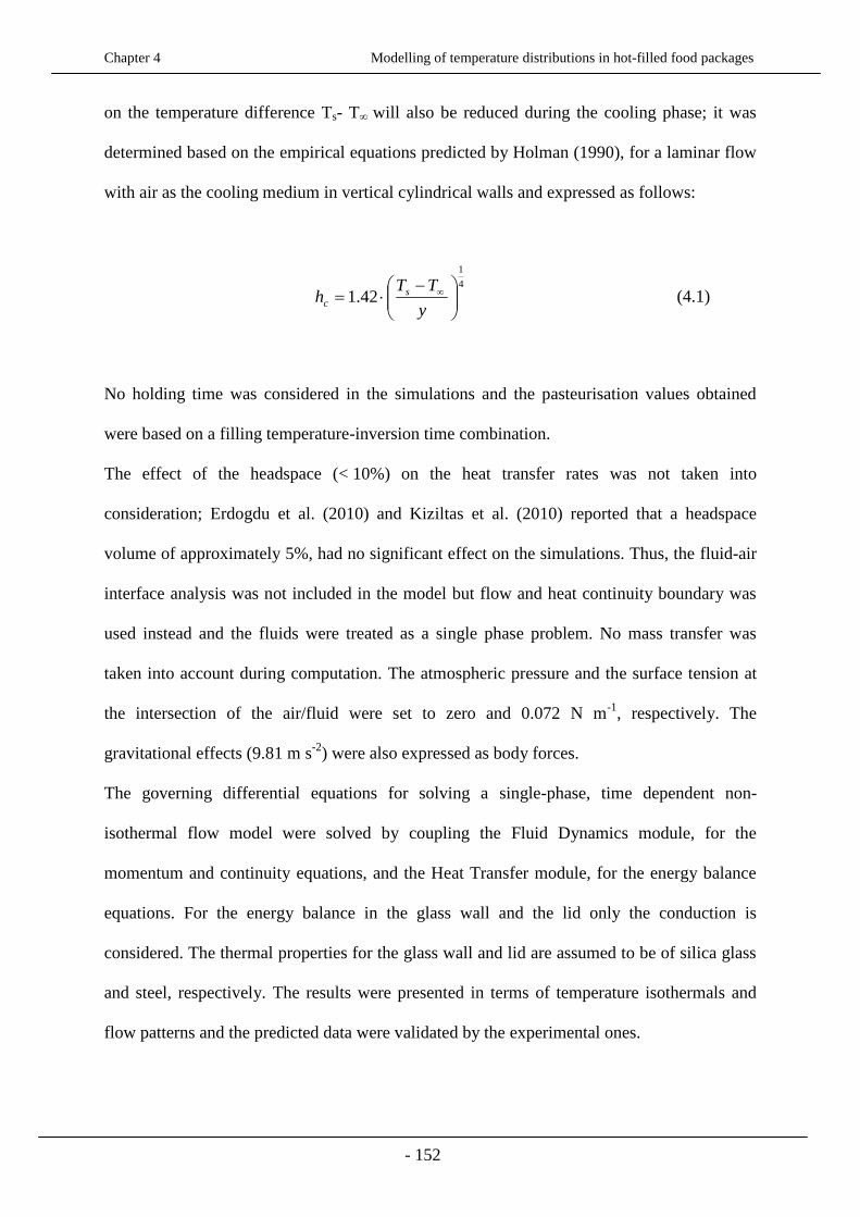
Chapter 4 Modelling of temperature distributions in hot-filled food packages
- 152
on the temperature difference Ts- T∞ will also be reduced during the cooling phase; it was
determined based on the empirical equations predicted by Holman (1990), for a laminar flow
with air as the cooling medium in vertical cylindrical walls and expressed as follows:
4
1
42.1
y
TTh s
c (4.1)
No holding time was considered in the simulations and the pasteurisation values obtained
were based on a filling temperature-inversion time combination.
The effect of the headspace (< 10%) on the heat transfer rates was not taken into
consideration; Erdogdu et al. (2010) and Kiziltas et al. (2010) reported that a headspace
volume of approximately 5%, had no significant effect on the simulations. Thus, the fluid-air
interface analysis was not included in the model but flow and heat continuity boundary was
used instead and the fluids were treated as a single phase problem. No mass transfer was
taken into account during computation. The atmospheric pressure and the surface tension at
the intersection of the air/fluid were set to zero and 0.072 N m-1
, respectively. The
gravitational effects (9.81 m s-2
) were also expressed as body forces.
The governing differential equations for solving a single-phase, time dependent non-
isothermal flow model were solved by coupling the Fluid Dynamics module, for the
momentum and continuity equations, and the Heat Transfer module, for the energy balance
equations. For the energy balance in the glass wall and the lid only the conduction is
considered. The thermal properties for the glass wall and lid are assumed to be of silica glass
and steel, respectively. The results were presented in terms of temperature isothermals and
flow patterns and the predicted data were validated by the experimental ones.
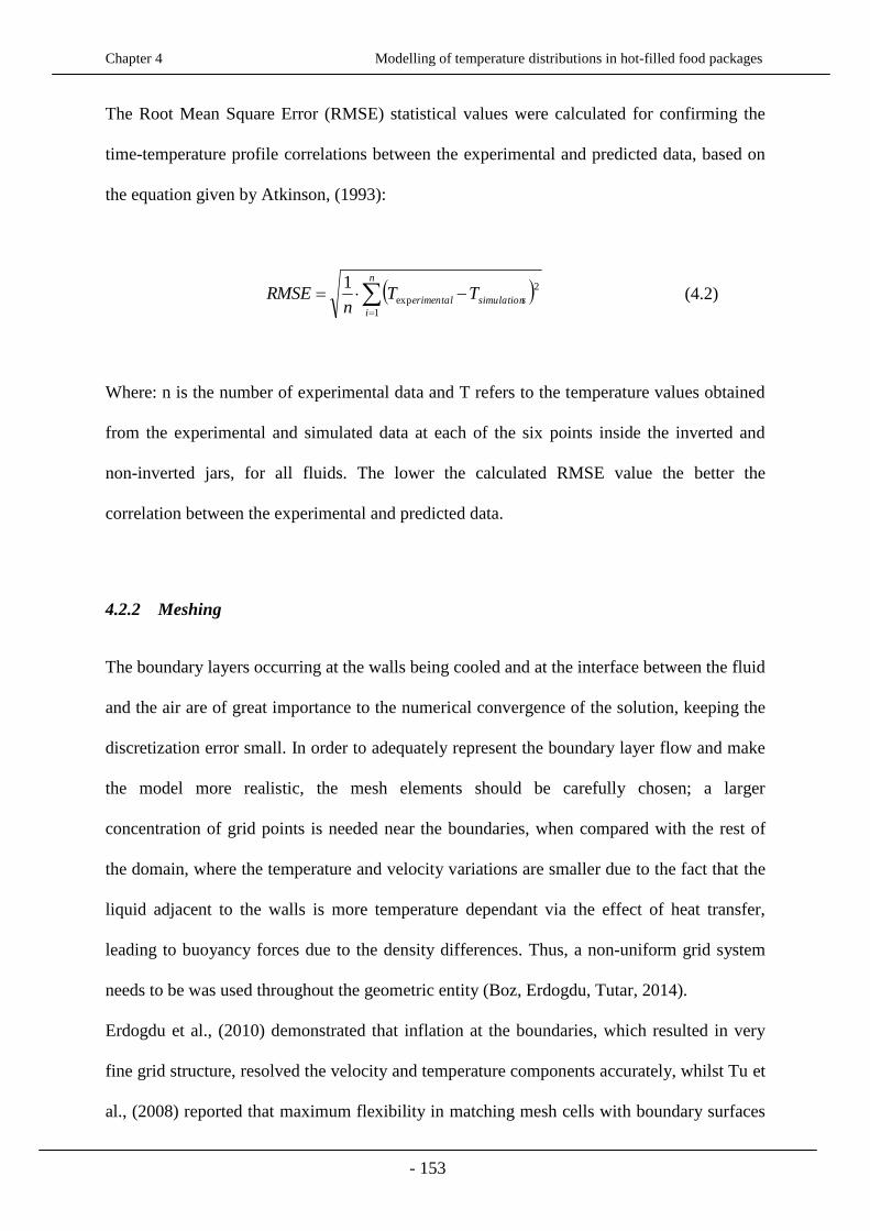
Chapter 4 Modelling of temperature distributions in hot-filled food packages
- 153
The Root Mean Square Error (RMSE) statistical values were calculated for confirming the
time-temperature profile correlations between the experimental and predicted data, based on
the equation given by Atkinson, (1993):
n
i
ssimulationerimental TTn
RMSE1
2
exp
1 (4.2)
Where: n is the number of experimental data and T refers to the temperature values obtained
from the experimental and simulated data at each of the six points inside the inverted and
non-inverted jars, for all fluids. The lower the calculated RMSE value the better the
correlation between the experimental and predicted data.
4.2.2 Meshing
The boundary layers occurring at the walls being cooled and at the interface between the fluid
and the air are of great importance to the numerical convergence of the solution, keeping the
discretization error small. In order to adequately represent the boundary layer flow and make
the model more realistic, the mesh elements should be carefully chosen; a larger
concentration of grid points is needed near the boundaries, when compared with the rest of
the domain, where the temperature and velocity variations are smaller due to the fact that the
liquid adjacent to the walls is more temperature dependant via the effect of heat transfer,
leading to buoyancy forces due to the density differences. Thus, a non-uniform grid system
needs to be was used throughout the geometric entity (Boz, Erdogdu, Tutar, 2014).
Erdogdu et al., (2010) demonstrated that inflation at the boundaries, which resulted in very
fine grid structure, resolved the velocity and temperature components accurately, whilst Tu et
al., (2008) reported that maximum flexibility in matching mesh cells with boundary surfaces
Chapter 4 Modelling of temperature distributions in hot-filled food packages
- 154
was achieved by the combination of different elements, such as triangular and quadrilateral
(hybrid grids); the quadrilateral or hexahedral elements were used to enhance the grid quality
at the boundary layers near the solid walls, while triangular or tetrahedral elements were used
for the rest of the flow domain for accurate solutions and faster convergence. Mesh
independency cannot always be achieved though, due to the restrictions in computational
power and time. For ensuring accuracy of the simulated results and mesh independency, 3
different mesh sizes, fine, finer and extra fine, were investigated and validated by the
experimental data at the wall, headspace and middle of the glass jar. The choice of the points
was made due to the difference in their mesh resolution; higher grid points are applied at the
boundaries, as compared to the less dense grid at the domain (Figure 4.2). The RMSE values
were calculated for demonstrating the differences between the mesh cases and the
experimental data. The value of the time step size used was 1 s.
4.2.3 Assumptions made for simplification
The following assumptions need to be made for defining the numerical problem and
simplifying it:
1. An axi-symmetric vertical geometry was selected in order to reduce the problem from
three-dimensional to two-dimensional; the computational time needed was significantly
reduced.
2. The thermal properties of the model fluids (specific heat (Cp), thermal conductivity (k),
and thermal expansion coefficient (β) are kept constant; temperature dependence of
density (ρ) is only used in the Boussinesq term.
3. The no-slip condition was applied at the inside walls of the jar, between the glass, lid
and the fluid.

Chapter 4 Modelling of temperature distributions in hot-filled food packages
- 155
4. The pressure within the fluid domain is unknown, making it difficult to achieve
convergence. Thus, the pressure was arbitrarily fixed at a point.
5. Heat generation due to viscous dissipation was considered to be negligible, due to the
low velocities of the highly viscous fluids used (Mills, 1995).
6. Boussinesq approximation is valid; the density difference has a linear relationship with
temperature.
7. The thermal boundary conditions are applied to the outer boundaries of the package, as
the thermal resistance of the glass and lid wall are taken into account.
8. The convective boundary condition, driven by the temperature difference between the
glass, lid and the surrounding atmosphere was applied in the simulations, at the top,
bottom, and side surfaces; no other thermal boundary condition was required for
describing the flow.
9. Laminar flow mode was assumed to hold through the whole cooling process.
4.2.4 Governing Equations
The study models the fluid motion with the incompressible Navier-Stokes equations since the
mass density remains more or less constant during motion and so the state equation can be
written as follows:
oxt , (4.3)
For ρο > 0 the mass conservation equation is expressed as:
0 (4.4)

Chapter 4 Modelling of temperature distributions in hot-filled food packages
- 156
The required governing equations of continuity, momentum and energy, in cylindrical
coordinates (Bird, Stewart & Lightfoot, 1960) are described as follows:
Continuity equation
01
v
zvr
rrfrf (4.5)
Energy equation
2
2
2
2
2
11
z
TT
rr
Tr
rrc
k
z
Tv
T
rr
Tv
t
T
fpf
f
zr
(4.6)
Momentum equation in vertical direction
gz
v
r
vr
rrz
P
z
vv
r
vv
t
vf
zzzz
zr
zf
2
21
(4.7)
Momentum equation in radial direction
2
21
z
vvr
rrrr
P
z
vv
r
vv
t
v rr
rz
rr
rf (4.8)
Where: T is temperature (oC), t is the cooling time (s), P is the pressure (Pa), g is the
gravitational acceleration (m s-2
), μ is the dynamic viscosity (Pa s), v is the velocity
component (m -s
1) and kf, cpf, and ρf are the thermal conductivity (Wm
-1 K
-1), the specific
heat (J kg-1
K-1
) and the density (kg m-3
) of the fluid, respectively. r, and z refer to the radial
and vertical axial direction, respectively.
The angular direction was not included in the momentum equation, since axi-symmetry was
assumed, reducing the computational time significantly. The ρf g term is assumed to be the
external force driving the natural convection process. The model treated the density as a
constant value in all solved equations except for the buoyancy term in the momentum

Chapter 4 Modelling of temperature distributions in hot-filled food packages
- 157
equation. Thus, the variation in density was neglected everywhere except in the buoyancy
term. The momentum equations were linearised and solved for a pressure set to zero. Energy
and flow equations were coupled to determine the heat transfer between water–air fluid side
and wall surface. The 1st-order numerical discretization scheme for the convection terms of
each governing equation and a 1st-order accurate implicit time integration scheme for time
discretization were used.
4.2.1.1 Boundary and Initial conditions
The initial and boundary conditions were obtained from the experimental results.
Initially, the fluid is at rest (u=0) and shows a uniform initial temperature:
T(r, z, t) = To =80oC (filling temperature);
u=0, v=0 at 0 ≤ r ≤ R, 0 ≤ z ≤ H+ x_lid
The boundary conditions used, were the following:
At the glass boundary, r=R:
T = Tgw, u=0, v=0, for 0 ≤ z ≤ H
At the glass bottom, z = 0:
T = Tgw, u=0, v=0, for 0 ≤ r ≤ R
At the top of the jar, where the boundary condition is applied at the lid, z = H + x_lid:
0
z
T, for 0 ≤ r ≤ R
At the symmetry:
0
r
T, for 0 ≤ z ≤ H+ x_lid

Chapter 4 Modelling of temperature distributions in hot-filled food packages
- 158
At the top and outer surfaces, the convective heat flux boundary condition was used, driven
by the temperature difference between the glass/lid and the surrounding atmosphere:
q=-h (T- Text) (4.9)
Where: q is the inward heat flux and h is the heat transfer coefficient of the surrounding air.
4.3 Results and Discussion
4.3.1 Meshing
According to Figures 4.2 and 4.3 for fluid A and T, respectively, a noticeable difference
between the three mesh resolutions and the experimental data was observed. It appears that
when finer and extra fine resolution was applied to the domain, the fluid structures near the
boundaries (walls and interface) increased the discretization of the flow equations and
apparently led to cumulative computational errors. The fine mesh size appeared to be the
most compatible with the experimental results. Another reason for the difference in mesh
resolutions could be the choice of the time step (1s) for the given convergence criterion
(Cornelissen et al., 2007). A more refined mesh should result in more accurate results, due to
the minimised discretization errors as compared to coarse or normal mesh resolutions.
Druzeta et al., (2009), reported that excessive mesh refinement could lead to deterioration of
the results because of faster accumulation of computational errors on higher mesh resolutions
caused by the Courant–Friedrichs–Lewy (CFL) condition. Breuer et al., (2000) explained this
contradiction using a filtering approach, which requires additional resources for time-
dependent laminar flows that bring resource limitations into the solution. If no filtering is
applied, as in the case of the current work, it is possible that modelling and discretization
errors will cancel each other leading to differences between mesh resolutions.

Chapter 4 Modelling of temperature distributions in hot-filled food packages
- 159
0 200 400 60074
75
76
77
78
79
80T
em
pera
ture
(oC
)
0 200 400 60071
72
73
74
75
76
77
78
79
80
time (s)
0 200 400 60040
45
50
55
60
65
70
75
80T
exp
fine mesh
finer mesh
extra fine mesh
i. ii. iii.
Figure 4.2: Comparison of predicted and experimental data obtained with fine, finer, extra fine mesh
resolution for fluid A at the: i. middle, ii. wall and iii. headspace.
0 200 400 60073
74
75
76
77
78
79
80
Tem
pera
ture
(oC
)
0 200 400 60066
68
70
72
74
76
78
80
time (s)
0 200 400 60040
45
50
55
60
65
70
75
80
Texp
fine mesh
finer mesh
extra fine mesh
I. II. III.
Figure 4.3: Comparison of predicted data obtained with fine, finer, extra fine mesh resolution and
experimental data for fluid T at the: I. middle, II. wall and III. headspace.

Chapter 4 Modelling of temperature distributions in hot-filled food packages
- 160
The differences observed between the mesh sizes applied, were confirmed by the calculation
of the RMSE values (Table 4.1). The more profound differences were shown to be between
the fine and extra fine resolution for the wall (up to 9 times higher) and the headspace (up to
15 times higher) of fluid A and T, respectively. That seems to confirm the above argument,
that the fluid structures near the boundaries lead to increased discretization and computational
errors. The difference at the middle is also noticeable for both fluids when the mesh is further
refined.
Table 4.1: RMSE values (oC) obtained from the three cases of mesh resolution.
Based on the above, fine grid was used for the domains of the fluid and air, with corner
refinement and triangular elements, whilst a layered quadrilateral mesh with finer grid was
used for the non-slip boundaries at the wall and bottom, which are subjected to sudden
changes over time, and at the interface of the coupled liquid-air system.
7031 nodal points were used with a finer grid in the domains and a finer grid near the wall
and the interface of fluid-air. The convergence criterion and the time step used was 10-8
and
1 second, respectively.
Fluids Location
within the jar
Fine Finer Extra fine
3% starch middle
wall headspace
0.17
0.16
1.24
1.03
1.28
3.42
1.17
1.41
4.26
Tomato soup middle
wall headspace
0.17
0.43
0.51
1.04
1.25
6.03
1.12
1.41
7.80
Chapter 4 Modelling of temperature distributions in hot-filled food packages
- 161
4.3.2 Heat treatment
Temperature isotherms and velocity fields were plotted to describe the temperature
distribution and the flow behaviour of 3% starch (A) and tomato soup (T) during the cooling
phase of the hot-fill treatment. The model fluids were examined for the two cases of non-
inverted (Case I) and inverted glass jars (Case II).
Case I: Fluid A
Figure 4.4 illustrates the temperature evolution of fluid (A), Case I at different cooling
periods of 1, 100 and 600 s; these times were arbitrarily chosen from the experimental results.
Initially, the fluid and the glass jar are at the same temperature, since the jars were preheated
before being hot-filled, and the headspace and the lid were set at an initial temperature of
20oC; the initial and boundary conditions were again chosen based on the experimental
results. During the hot-filling, the fluid starts cooling through the walls and moves
downwards, as the density near the walls increases. The core of the fluid, which is the slowest
cooling point in the jar (the furthest from the walls) remains at high temperature and moves
upwards heating up the headspace and the lid (Figure 4.4 a). The process time (10 min) is not
sufficient to enable the hot regions of the fluid to cool down significantly; approximately 1.5
hours of processing time was needed for the bulk of the fluids to reach the medium (air)
temperature (20oC). The hot fluid moving upwards is deflected by the lid and starts moving in
radial direction, downwards as it gets heavier. The headspace is heated instantaneously (in
the first 5 seconds, Figure 4.4 a) whilst the lid starts being heated at approximately 100
seconds (Figure 4.4 b). At the end of the process the dominating effect of conduction is
clearly demonstrated (Figure 4.4 c), with convection occurring only through the latter
boundaries. That is due to the relatively high viscosity of the fluid and the short process time,
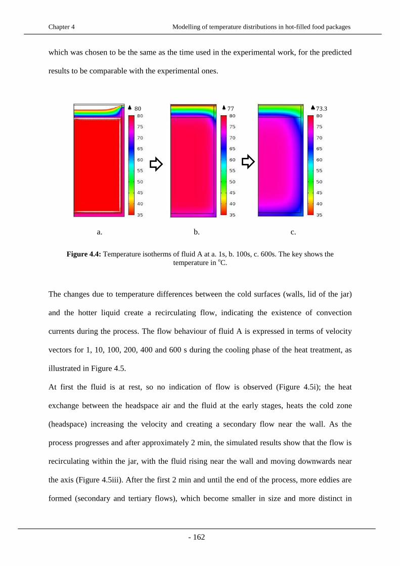
Chapter 4 Modelling of temperature distributions in hot-filled food packages
- 162
which was chosen to be the same as the time used in the experimental work, for the predicted
results to be comparable with the experimental ones.
a. b. c.
Figure 4.4: Temperature isotherms of fluid A at a. 1s, b. 100s, c. 600s. The key shows the
temperature in oC.
The changes due to temperature differences between the cold surfaces (walls, lid of the jar)
and the hotter liquid create a recirculating flow, indicating the existence of convection
currents during the process. The flow behaviour of fluid A is expressed in terms of velocity
vectors for 1, 10, 100, 200, 400 and 600 s during the cooling phase of the heat treatment, as
illustrated in Figure 4.5.
At first the fluid is at rest, so no indication of flow is observed (Figure 4.5i); the heat
exchange between the headspace air and the fluid at the early stages, heats the cold zone
(headspace) increasing the velocity and creating a secondary flow near the wall. As the
process progresses and after approximately 2 min, the simulated results show that the flow is
recirculating within the jar, with the fluid rising near the wall and moving downwards near
the axis (Figure 4.5iii). After the first 2 min and until the end of the process, more eddies are
formed (secondary and tertiary flows), which become smaller in size and more distinct in
80 77 73.3
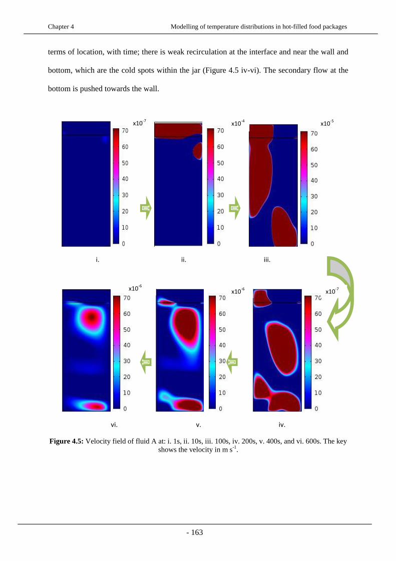
Chapter 4 Modelling of temperature distributions in hot-filled food packages
- 163
terms of location, with time; there is weak recirculation at the interface and near the wall and
bottom, which are the cold spots within the jar (Figure 4.5 iv-vi). The secondary flow at the
bottom is pushed towards the wall.
i. ii. iii.
vi. v. iv.
Figure 4.5: Velocity field of fluid A at: i. 1s, ii. 10s, iii. 100s, iv. 200s, v. 400s, and vi. 600s. The key
shows the velocity in m s-1
.
x10-7
x10-5
x10-6
x10-6
x10-7
x10-4

Chapter 4 Modelling of temperature distributions in hot-filled food packages
- 164
Case I: Fluid T
The observations made from the temperature isotherms of fluid T (Figure 4.6) were similar to
the ones from fluid A; the headspace is being heated instantaneously (Figure 4.6a) whilst it
takes approximately 180 s for the lid to be heated. The highest temperatures reached at the
bulk of the fluid, are higher than those observed for fluid A, which is expected, since the
tomato soup cools down slower.
A. B. C.
Figure 4.6: Temperature isotherms of fluid T at a. 1s, b. 100s, c. 600s. The key shows the temperature
in oC.
The velocity field plotted for describing the flow of tomato soup (Figure 4.7) indicates that
the fluid seems to be at rest for the first 70-80 seconds with the temperature being uniform at
this stage and then gradually, as the cooling progresses convection currents become evident at
the boundaries. That is illustrated by the movement of the cold zone close to the interface,
towards the bottom of the container. The cold spot continues to move until it eventually
remains at a region that is about 20% from the bottom of the jar.
Studies carried out by Datta and Texeira, (1987) on the sterilisation of cans consisting of a
viscous fluid such as CMC (carboxy-methyl cellulose), showed that a secondary flow is
80 79 74.8
Chapter 4 Modelling of temperature distributions in hot-filled food packages
- 165
formed at the bottom of the can, near the centre line, whilst later on, Kumar and Bhattachary,
(1991) simulated the same fluid but no secondary zones were indicated. From the simulation
obtained in the current work, the formation of eddies was evident in both fluids, with tomato
soup having similar viscosity with CMC (≈1 Pa s at a reference temperature of 80oC, based
on Equation 3.3, Chapter 3 § 3.2.) and the starch solution with a value of ≈ 0.3Pa s,
confirming the findings of the Datta and Texeira. However, the results in this work refer to
the cooling effect on the fluid behaviour instead of heating. Thus, more research needs to be
conducted for testing the similarities of the heating and cooling effect on the formation of
secondary zones. Kumar and Bhattacharya (1991) reported that the thickness of ascending
viscous liquids (CMC) near the wall (the distance between the location of the stagnant region
and the wall) in the case of cans’ sterilisation was greater (12 mm) than that for water
(6 mm), attributed to the large viscosity difference between the two fluids.
According to calculations made upon actual container dimensions, the thickness of the starch
solutions and the tomato soup was 3 and 4 mm, respectively. The difference in thickness is
not significant, since the viscosity difference is not sufficiently large and it can explain the
small differences observed in flow behaviour between the two fluids.
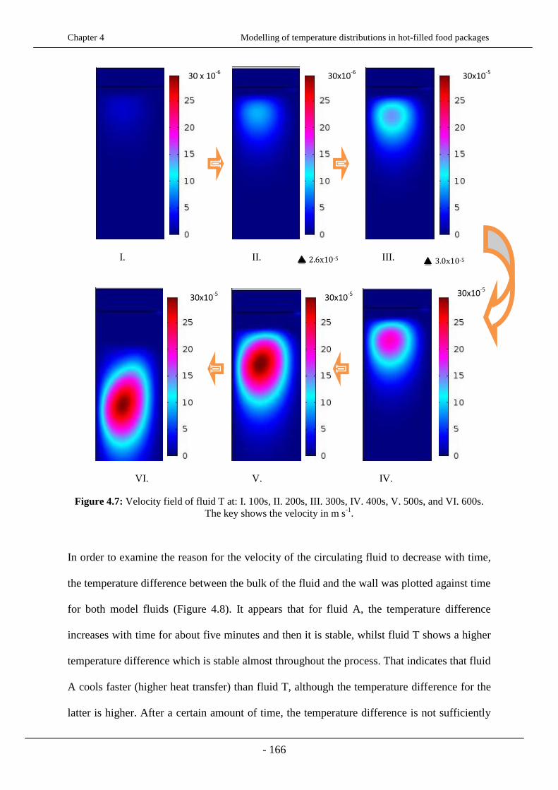
Chapter 4 Modelling of temperature distributions in hot-filled food packages
- 166
I. II. III.
VI. V. IV.
Figure 4.7: Velocity field of fluid T at: I. 100s, II. 200s, III. 300s, IV. 400s, V. 500s, and VI. 600s.
The key shows the velocity in m s-1
.
In order to examine the reason for the velocity of the circulating fluid to decrease with time,
the temperature difference between the bulk of the fluid and the wall was plotted against time
for both model fluids (Figure 4.8). It appears that for fluid A, the temperature difference
increases with time for about five minutes and then it is stable, whilst fluid T shows a higher
temperature difference which is stable almost throughout the process. That indicates that fluid
A cools faster (higher heat transfer) than fluid T, although the temperature difference for the
latter is higher. After a certain amount of time, the temperature difference is not sufficiently
3.0x10⁻⁵ 2.6x10⁻⁵
30 x 10-6
30x10-6
30x10-5
30x10-5
30x10-5 30x10
-5
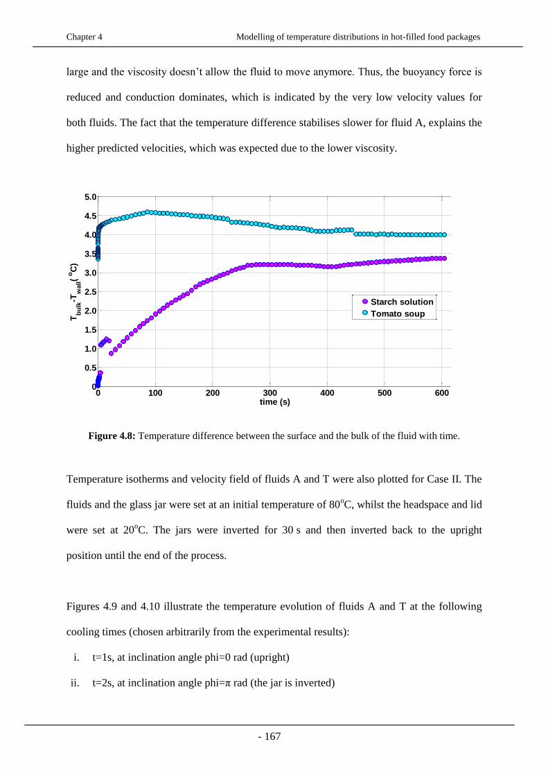
Chapter 4 Modelling of temperature distributions in hot-filled food packages
- 167
large and the viscosity doesn’t allow the fluid to move anymore. Thus, the buoyancy force is
reduced and conduction dominates, which is indicated by the very low velocity values for
both fluids. The fact that the temperature difference stabilises slower for fluid A, explains the
higher predicted velocities, which was expected due to the lower viscosity.
0 100 200 300 400 500 6000
0.5
1.0
1.5
2.0
2.5
3.0
3.5
4.0
4.5
5.0
time (s)
Tb
ulk
-Tw
all(
oC
)
Starch solution
Tomato soup
Figure 4.8: Temperature difference between the surface and the bulk of the fluid with time.
Temperature isotherms and velocity field of fluids A and T were also plotted for Case II. The
fluids and the glass jar were set at an initial temperature of 80oC, whilst the headspace and lid
were set at 20oC. The jars were inverted for 30 s and then inverted back to the upright
position until the end of the process.
Figures 4.9 and 4.10 illustrate the temperature evolution of fluids A and T at the following
cooling times (chosen arbitrarily from the experimental results):
i. t=1s, at inclination angle phi=0 rad (upright)
ii. t=2s, at inclination angle phi=π rad (the jar is inverted)
Chapter 4 Modelling of temperature distributions in hot-filled food packages
- 168
iii. t=32s, at inclination angle phi=π rad (at the end of inversion)
iv. t=33s, at inclination angle phi=2π rad (after the 2nd
inversion), and
v. t=600s, at inclination angle phi=2π rad, at the end of the process
Case II: Fluid A
Initially, the jar is cooling down from the walls creating a flow downwards, while the bulk of
the fluid flows upwards heating up the headspace. Once the jar is inverted, the headspace and
the lid show a temperature increase of approximately 20oC, whilst close to the interface of
fluid-air and at the centreline (Figure 4.9b) the fluid flow is disrupted and a decrease in
temperature is observed. The forced convection caused by inverting the jars, created
recirculating zones within the fluid and especialy near the boundaries. The disruption
observed at the interface and near the wall could in reality be because of an existing bubble or
the coldzone movement from the headspace towards the bottom of the jar.
At the end of the first inversion, after 30 s at an inclination angle of π rad (Figure 4.9c), the
headspace and lid become hotter, whilst the temperature of the bottom starts decreasing.
When the jar is inverted again at the upright position, it seems that the cold zone moved from
the headspace, towards the bottom and then appears close to the interface and right wall. That
could theoretically support the existence of bubbles during the process, but cannot be
described numerically with the single-phase flow module used in the current work; air and
fluid would have to be treated as a two phase-model system. By the end of the process, the
flow reaches stability and whist the bulk of the fluid is conduction-dominated, the interface
and walls are convection dominated.

Chapter 4 Modelling of temperature distributions in hot-filled food packages
- 169
a. b. c.
e. d.
Figure 4.9: Temperature isotherms of fluid A at a. 1s, b. 2s, c. 32s, d. 33s and e. 600s.
The observations made from the temperature isotherms are reflected in the velocity field
plots. Initially, the headspace air mixes with the fluid and moves towards the bottom of the
container, creating at the end of the first inversion secondary and tertiary flows near the axis
and at the bottom wall of the jar. By inverting the jar upright, the fluid flows over the whole
surface of the jar relatively fast, and then once it mixes with the headspace air again, it is
separated into two main flows, covering the colder zones of the headspace and the bottom
wall and a third one close to the interface and right side wall (Figure 4.10 C-D). After
approximately two minutes, there are two distinct flows; the cold zones of both the headspace
80 79. 4 79.0
73.2 78.3
Lid
Lid
Lid

Chapter 4 Modelling of temperature distributions in hot-filled food packages
- 170
and the bottom are pushed towards the wall, with their size being decreased (velocity
significantly reduced).
A. B. C. D.
H. G. F. E.
Figure 4.10: Velocity field of fluid A at: A. 1s, B. 30s, C. 31s, D. 100s, E. 300s, F. 400s, G. 500s,
H. 600s.
Lid
Lid
35x10-4
35x10-4
35x10-3
35x10-4
35x10-5
35x10-5
35x10-5
35x10-5

Chapter 4 Modelling of temperature distributions in hot-filled food packages
- 171
Case II: Fluid T
In the isotherms concerning the tomato soup, the observations are similar to the ones
concerning the starch solution, except from the slightly higher temperatures recorded due to
the slower cooling of the fluid. Convection occurs through the walls and the interface, whilst
the bulk of the fluid is mostly conduction dominated. By inverting the jars, the temperature of
the headspace and the lid is increased, whilst it is decreased at the bottom and the interface,
since the fluid is mixed with the headspace air (Figure 4.11ii). The interface is also disrupted
in the case of fluid T, indicating the heat exchange between hot and cold zones, but it is less
profound than in fluid A which would be expected from the lower viscosity and consequently
the lower velocities occuring. At the end of the first inversion (Figure 4.11iii), the headspace
and lid reach their highest temperature, whilst the bottom reaches its lowest. The flow
becomes more stable after approximately six minutes, no more disruptions at the interface
and the walls, with the bulk of the fluid being dominated by conduction and the latter
boundaries being responsible for the laminar convection.
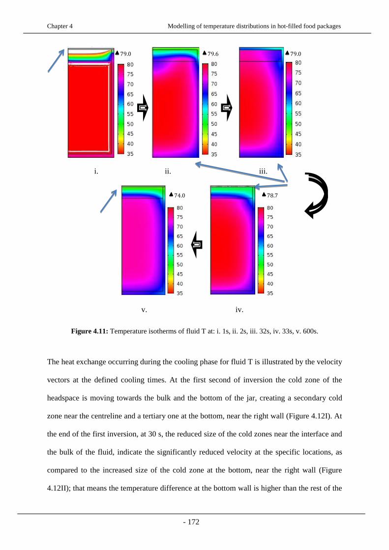
Chapter 4 Modelling of temperature distributions in hot-filled food packages
- 172
i. ii. iii.
v. iv.
Figure 4.11: Temperature isotherms of fluid T at: i. 1s, ii. 2s, iii. 32s, iv. 33s, v. 600s.
The heat exchange occurring during the cooling phase for fluid T is illustrated by the velocity
vectors at the defined cooling times. At the first second of inversion the cold zone of the
headspace is moving towards the bulk and the bottom of the jar, creating a secondary cold
zone near the centreline and a tertiary one at the bottom, near the right wall (Figure 4.12I). At
the end of the first inversion, at 30 s, the reduced size of the cold zones near the interface and
the bulk of the fluid, indicate the significantly reduced velocity at the specific locations, as
compared to the increased size of the cold zone at the bottom, near the right wall (Figure
4.12II); that means the temperature difference at the bottom wall is higher than the rest of the
79.0 79.6 79.0
74.0 78.7
Lid
Lid
Lid

Chapter 4 Modelling of temperature distributions in hot-filled food packages
- 173
fluid at the specific time. When the container is inverted again to the upright position, there is
an increased velocity throughout the fluid, shown by the bulk movement over most of the jar
surface (Figure 4.12III). At approximately the first three minutes after the jar is inverted
upright, a low velocity secondary flow is formed at the headspace, near the lid, whilst big part
of the rest of the flow is moving downwards, until it reaches the bottom wall. The rest of the
time until the end of the process, the velocity of the cold zone at the bottom wall is gradually
reduced, until the fluid finally stops circulating at that point whilst at the meantime, a
secondary flow is formed again at the headspace, increasing with time. The results reflect the
observation from the temperature isotherms, since the velocity plots show that the cold spots
are located near the interface and the walls.

Chapter 4 Modelling of temperature distributions in hot-filled food packages
- 174
I. II. III. IV. V.
IX. VIII. VII. VI.
Figure 4.12: Velocity field of fluid T at I.1s, II. 30s, III. 31s, IV. 50s, V. 100s, VI. 200s, VII. 400s,
VIII. 600s.
4.3.3 Model validation
The predicted time-temperature data were validated by being compared with the experimental
data for both cases and fluids. The RMSE values were calculated for confirming the time-
temperature profile correlations between the experimental and predicted data, presented in
Table 4.2, based on equation 4.2.
Lid
Lid
100x10-8
100x10-7 100x10
-7 100x10
-6
25x10-4 25x10
-4 100x10
-5
100x10-5
100x10-6
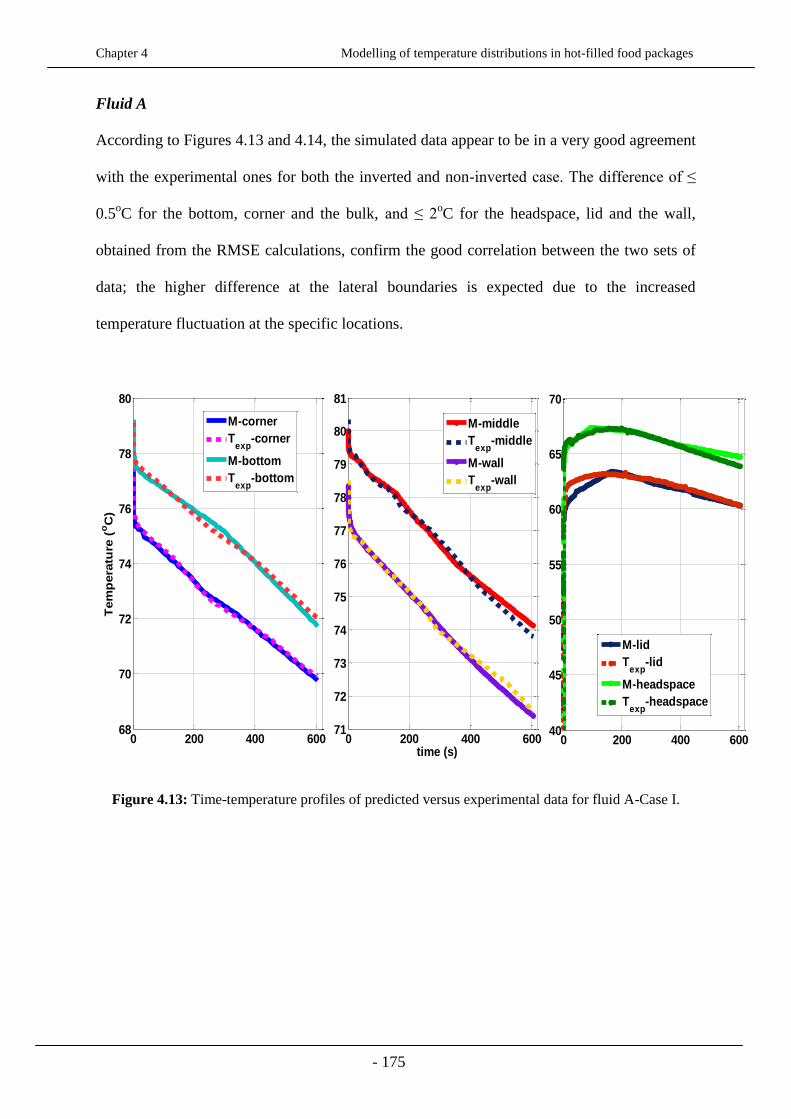
Chapter 4 Modelling of temperature distributions in hot-filled food packages
- 175
Fluid A
According to Figures 4.13 and 4.14, the simulated data appear to be in a very good agreement
with the experimental ones for both the inverted and non-inverted case. The difference of ≤
0.5oC for the bottom, corner and the bulk, and ≤ 2
oC for the headspace, lid and the wall,
obtained from the RMSE calculations, confirm the good correlation between the two sets of
data; the higher difference at the lateral boundaries is expected due to the increased
temperature fluctuation at the specific locations.
0 200 400 60068
70
72
74
76
78
80
time (s)
Tem
pera
ture
(oC
)
0 200 400 60071
72
73
74
75
76
77
78
79
80
81
0 200 400 60040
45
50
55
60
65
70
M-corner
Texp
-corner
M-bottom
Texp
-bottom
M-middle
Texp
-middle
M-wall
Texp
-wall
M-lid
Texp
-lid
M-headspace
Texp
-headspace
Figure 4.13: Time-temperature profiles of predicted versus experimental data for fluid A-Case I.
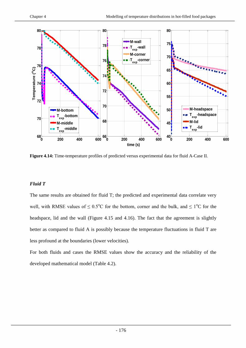
Chapter 4 Modelling of temperature distributions in hot-filled food packages
- 176
0 200 400 60068
70
72
74
76
78
80T
em
pera
ture
(oC
)
0 200 400 60066
68
70
72
74
76
78
80
time (s)
0 200 400 60040
45
50
55
60
65
70
75
80
M-bottom
Texp
-bottom
M-middle
Texp
-middle
M-wall
Texp
-wall
M-corner
Texp
-corner
M-headspace
Texp
-headspace
M-lid
Texp
-lid
Figure 4.14: Time-temperature profiles of predicted versus experimental data for fluid A-Case II.
Fluid T
The same results are obtained for fluid T; the predicted and experimental data correlate very
well, with RMSE values of ≤ 0.5oC for the bottom, corner and the bulk, and ≤ 1
oC for the
headspace, lid and the wall (Figure 4.15 and 4.16). The fact that the agreement is slightly
better as compared to fluid A is possibly because the temperature fluctuations in fluid T are
less profound at the boundaries (lower velocities).
For both fluids and cases the RMSE values show the accuracy and the reliability of the
developed mathematical model (Table 4.2).
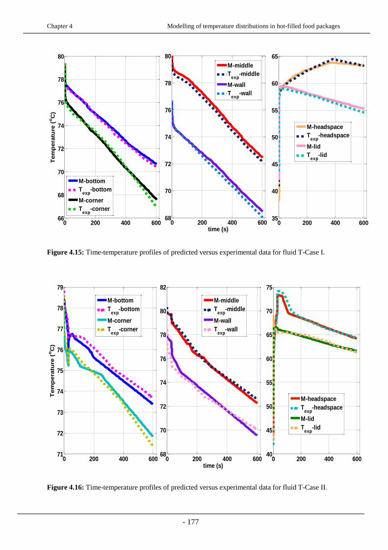
Chapter 4 Modelling of temperature distributions in hot-filled food packages
- 177
0 200 400 60066
68
70
72
74
76
78
80T
em
pera
ture
(oC
)
0 200 400 60068
70
72
74
76
78
80
time (s)
0 200 400 60035
40
45
50
55
60
65
M-bottom
Texp
-bottom
M-corner
Texp
-corner
M-headspace
Texp
-headspace
M-lid
Texp
-lid
M-middle
Texp
-middle
M-wall
Texp
-wall
Figure 4.15: Time-temperature profiles of predicted versus experimental data for fluid T-Case I.
0 200 400 60071
72
73
74
75
76
77
78
79
Tem
pera
ture
(oC
)
0 200 400 60068
70
72
74
76
78
80
82
time (s)
0 200 400 60040
45
50
55
60
65
70
75
M-headspace
Texp
-headspace
M-lid
Texp
-lid
M-bottom
Texp
-bottom
M-corner
Texp
-corner
M-middle
Texp
-middle
M-wall
Texp
-wall
Figure 4.16: Time-temperature profiles of predicted versus experimental data for fluid T-Case II.
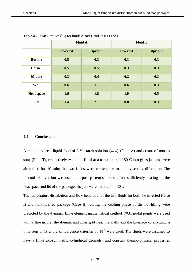
Chapter 4 Modelling of temperature distributions in hot-filled food packages
- 178
Table 4.2: RMSE values (oC) for fluids A and T and Cases I and II.
Fluid A Fluid T
Inverted Upright Inverted Upright
Bottom 0.5 0.3 0.3 0.3
Corner 0.5 0.5 0.3 0.3
Middle 0.3 0.4 0.2 0.3
Wall 0.6 1.1 0.6 0.3
Headspace 1.6 1.8 1.0 0.5
lid 1.4 2.1 0.8 0.3
4.4 Conclusions
A model and real liquid food of 3 % starch solution (w/w) (Fluid A) and cream of tomato
soup (Fluid T), respectively, were hot-filled at a temperature of 80oC into glass jars and were
air-cooled for 10 min; the two fluids were chosen due to their viscosity difference. The
method of inversion was used as a post-pasteurisation step for sufficiently heating up the
headspace and lid of the package; the jars were inverted for 30 s.
The temperature distribution and flow behaviour of the two fluids for both the inverted (Case
I) and non-inverted package (Case II), during the cooling phase of the hot-filling were
predicted by the dynamic finite element mathematical method. 7031 nodal points were used
with a fine grid at the domain and finer grid near the walls and the interface of air-fluid; a
time step of 1s and a convergence criterion of 10-8
were used. The fluids were assumed to
have a finite axi-symmetric cylindrical geometry and constant thermo-physical properties
Chapter 4 Modelling of temperature distributions in hot-filled food packages
- 179
(thermal conductivity k, specific heat Cp, thermal expansion coefficient b, and density); the
density was assumed to be constant in the governing equations except in the buoyancy term,
where the Boussinesq approximation is used, for describing its variation with temperature.
The viscosity was modelled as a as temperature dependant variable.
The inversion step was numerically solved by the use of a parametric sweep step which
simulated the temperature distribution at inclination angles (angle of the gravity vector from
its initial vertical position) from 0 to π rad for the first inversion (upright to inverted
position), and from π to 2π rad (inverted to upright position again) for the second inversion.
The temperature isotherms plotted for illustrating the temperature evolution during the
cooling phase of the treatment show that the fluid is rapidly cooled down near the walls
creating a downward flow, whilst the core remains at high temperatures and moves upwards,
heating up the headspace and the lid; that created recirculation zones which were reflected in
the velocity plots. In both fluids and cases, the cold zones are located near the walls and the
interface between the fluid and air. The convection currents push the cold zones of the fluid
to move from the headspace towards the bottom of the jar and near the wall, creating
secondary and tertiary flows. The forced convection caused by the inversion of the package,
created higher recirculation within the fluid; the disrupted interface of the fluids indicated the
existence of either a bubble, created during inversion or the movement of cold spots within
the fluid. The velocity plots showed faster heat transfer in fluid A, with the velocities being
up to ten times higher than those in fluid T. The comparison of the predicted temperature
profiles with the experimental ones showed good agreement for both cases and fluids. The
correlation of the two data sets was confirmed by the low RMSE values obtained.
The validation of the mathematical model developed, makes the future design, control and
optimisation of thermal processes promising.
Chapter 4 Modelling of temperature distributions in hot-filled food packages
- 180
References
Atkinson K., (1993). Elementary Numerical Analysis (2nd
ed.). John Wiley & Sons, Inc.,
New York, NY, USA (Chapter 8).
Avila I.M.L.B., Silva, C.L.M. (1999). Modelling kinetics of thermal degradation of colour of
peach puree. Journal of Food Engineering, 39, 161–166.
Boz Z., Erdogdu F., Tutar M., (2014). Effects of mesh refinement, time step size and
numerical scheme on the computational modeling of temperature evolution during natural-
convection heating. Journal of Food Engineering, 123, 8–16.
Breuer M., (2000). A challenging test case for the large eddy simulation: high Reynolds
number circular cylinder flow. International Journal of Heat and Fluid Flow, 21, 648–654.
Bukhari S.J.K., Siddiqui M.H.K., (2007). Characteristics of air and water velocity fields
during natural convection. Heat Mass Transfer, 43, 5, 415-425.
Cornelissen J.T., Taghipour F., Escudie R., Ellisa N., Grace J.R., (2007). CFD modelling of a
liquid–solid fluidized bed. Chemical Engineering Science, 62, 6334–6348.
Cox P.W. and Fryer P.J., (2002). Modelling thermal processes: heating. Food process
modelling, 340–364.
Datta A.K., Teixeira A.A., (1987). Numerical modelling of natural convection heating in
canned liquid foods. Transactions of American Society of Agricultural Engineers, St. Joseph,
MI: American Society of Agricultural Engineers.
Datta A.K., Teixeira, A.A., (1988). Numerically predicted transient temperature and velocity
profiles during natural convection heating of canned liquid foods. Journal of Food Science,
53 (1), 191-195.
Druzeta S., Sopta L., Macesic S., Crnjaric-Zic N., (2009). Investigation of the importance of
spatial resolution for two-dimensional shallow-water model accuracy. Journal of Hydraulic
Engineering 11, 917–925.
Erdogdu F., Uyar R., Palazoglu T.K., (2010). Experimental comparison of natural convection
and conduction heat transfer. Journal of Food Process Engineering, 33, 85–100.
Erdogdu F., Tutar M., (2011). Velocity and temperature field characteristics of water and air
during natural convection heating in cans. Journal of Food Science, 76, 119–129.
Ghani A.A.G., Farid M.M., Chen X.D., Richards P., (1999). Numerical simulation of natural
convection heating of canned food by computational fluid dynamics. Journal of Food
Engineering, 41, 55–64.

Chapter 4 Modelling of temperature distributions in hot-filled food packages
- 181
Ghani A.A.G., Farid M.M., Chen X.D., Richards P., (1999). An investigation of deactivation
of bacteria in a canned liquid food during sterilization using computational fluid dynamics
(CFD). Journal of Food Engineering, 42, 207-214.
Ghani A.A.G., Farid M.M., Chen X.D., (2002). Numerical simulation of transient
temperature and velocity profiles in a horizontal can during sterilization using computational
fluid dynamics. Journal of Food Engineering, 51, 77–83.
Ghani A.G., Farid M.M., (2006). Using the computational fluid dynamics to analyse the
thermal sterilization of solid–liquid food mixture in cans. Innovative Food Science Emerging
Technologies, 7, 55–61.
Holman J. P., (1992). Heat transfer, UK: McGraw-Hill.
Joseph S.J., Speers R.A., Pillay V., (1996). Effect of head space variation and heat treatment
on the thermal and rheological properties of non-agitated, conduction-heated materials.
Lebensm Wiss u. Technologie, 29, 556–560.
Kannan A., Sandaka P.Ch.G., (2008). Heat transfer analysis of canned food in a still retort.
Journal of Food Engineering, 88, 213–228.
Kiziltas S., Erdogdu F., Palazoglu T.K., (2010). Simulation of heat transfer for solid–liquid
food mixtures in cans 3 and model validation under pasteurization conditions. Journal of
Food Engineering, 97, 449–456.
Kumar A., Bhattacharya M., Blaylock J., (1990). Numerical simulation of natural convection
heating of canned thick viscous liquid food products. Journal of Food Science, 55, 1403–
1411, 1420.
Kumar A., Bhattacharya M., (1991). Transient temperature and velocity profiles in a canned
non-Newtonian liquid food during sterilization in a still-cook retort. International Journal of
Heat and Mass Transfer, 34, 1083–1096.
Mills A.F., (1995). Basic heat and mass transfer, USA: Irwin.
Moraga N., Torres A., Guarda A., Galotto M.J., (2011). Non-Newtonian canned liquid food,
unsteady fluid mechanics and heat transfer prediction for pasteurization and sterilization.
Journal of Food Process Engineering, 34, 2000–2025.
Mohamed I.O., (2007). Determination of an effective heat transfer coefficients for can
headspace during thermal sterilization process. Journal of Food Engineering, 79, 1166–1171. Ramaswamy S., Grabowski S., (1996). Influence of entrapped air on the heating behaviour of
a model food packaged in semi-rigid plastic containers during thermal processing. Food
Science Technology, 29, 82–93.
Sandoval, Barreiro, Mendoza, (1994). Prediction of hot-fill-air-cool sterilization processes for
tomato paste in glass jars. Journal of Food Engineering 23, 33–50.

Chapter 4 Modelling of temperature distributions in hot-filled food packages
- 182
Teixeira A.A., (1992). Food Engineering Handbook: Thermal process calculations. Marcel
Dekker, Inc, New York, NY, 563-619.
Tu J., Yeoh G.H., Liu C., (2008). Computational Fluid Dynamics: A Practical Approach.
Elsevier Applied Science Publishers, New York, NY, USA, p. 36.
Tutar M., Erdogdu F., (2012). Numerical simulation for heat transfer and velocity field
characteristics of two-phase flow systems in axially rotating horizontal cans. Journal of Food
Engineering, 111, 366–385.
Weintraub S.E., Ramaswamy H.S., Tung M.A., (1989). Heating rates in flexible packages
containing entrapped air during overpressure processing. Journal of Food Science, 54, 1417–
1421.
Chapter 5 TTI validation for hot-fill processes
- 183
Chapter 5 - TTI validation for hot-fill processes
Abstract
Traditionally, thermal processes are quantified by using temperature sensors (thermocouples).
However, in processes where complexities such as particulate foods or continuously cooked
products are introduced, the application of thermocouples is not convenient and the process
validation can be challenging.
The use of time temperature integrators (TTIs) as an alternative means to process evaluation
of either temperature or microbial systems has recently received considerable attention (Van
Loey, & Hendrickx, 2002). In the current chapter, TTIs were tested for their reliability and
accuracy under isothermal and non-isothermal conditions, and were then used for the
validation of the hot-fill process, for a target process of 2 min at 70oC (Target I) and 5 min at
85oC (Target II). The TTI systems used in the following experiments are based on α-amylase
from Bacillus amyloliquefaciens (BAA) prepared as two different solutions for evaluating the
two target processes at the reference temperatures of 70 and 85oC, referred to as BAA70 and
BAA85, respectively. When tested under isothermal conditions, the TTIs resulted in a D70-
value of 4.1 min and a z-value of 10.8oC for BAA70 and a D85-value of 8.7 and a z-value of
10.3oC for BAA85; the heat duration was calculated to be 7 and 16 min for BAA70 and
BAA85, respectively.
A Peltier stage was used for investigating the response of the two TTI systems under non-
isothermal conditions. The TTIs appeared to be reliable in picking up small temperature

Chapter 5 TTI validation for hot-fill processes
- 184
differences, but they cannot reach the temperature that the Peltier stage is set to deliver.
Finally, their response was investigated under hot-fill treatments and was compared to that of
the thermocouples, subjected to the same thermal treatments. The heating mediums used for
the thermal process were water, 3% starch solution and tomato soup; the process values were
obtained at five locations inside the glass jar, the bottom, corner, wall, headspace and the lid.
The target process was achieved by the bottom, bottom-corner and wall for BAA70 TTI and
all three fluids, but he filling temperature was not sufficient to pasteurise the headspace and
the lid. Both TTI systems record lower temperatures than thermocouples under any of the
conditions they were submitted in the current work.
A statistical analysis was performed for illustrating how significantly different the two
monitoring techniques are; results obtained from ANOVA showed that the two methods are
not significantly different at a 5% confidence level and that given the potential for
discrepancy, the TTI systems could be safely used for evaluating pasteurisation processes.
5.1 Introduction
Food thermal processing is still one of the most widely used food preservation methods
aiming to deliver safe food to the consumer, by inactivating the pathogenic micro-organisms
within it, and to extend the foods’ shelf life (Bellara et al., 1999).
As the variety of food products, processes and container types is increasing, food
manufacturers are faced with the challenge of proving that their products are microbially safe.
Consumers’ awareness of healthy food and the tighter regulations in terms of additives
maximise the challenge of food producers, since the product delivered to the consumer needs
to be safe and of high quality at the same time; this is an optimisation problem. Thus, the
validation of thermal processes has become of ever-increasing importance. The use of
Chapter 5 TTI validation for hot-fill processes
- 185
conventional temperature probes is the most common method of validating thermal
processes, since they are accurate over a defined temperature range and are sensitive to
temperature change. However, they are not always convenient to be used due to complexities
introduced by products cooked in continuous ovens, such as poultry joints, burgers and bread,
and products with discrete pieces cooked in agitated vessels or heat exchangers such as ready
meals, soups, cook-in-sauces, and dressings (Tucker, 2003). Because of the above mentioned
complexities, other monitoring techniques need to be adopted for evaluating the impact of a
heat treatment on safety and quality of a food product.
Alternative options available are the following:
o Microbiological methods: they are divided into the count reduction method, which
refers to the inoculation of the entire food with organisms of known heat resistance, and the
method of spores encapsulated in an alginate bead. The bead mimics the food pieces in their
thermal and physical behaviour so that its heating rate is similar to the food (Brown et al.,
1984). The method relies on the measurement of the log reductions obtained by enumerating
the surviving organisms or spores, which are converted into process values.
o The in situ method: the approach relies on the direct evaluation of a quality attribute
such as colour and vitamin content, before and after the thermal treatment. Detection limits,
sample size requirements, in the case of inactivation of microorganisms and their spores, and
recontamination are examples of the method having a restricted application (Mulley et al.,
1975).
o The physical-mathematical approach: it is frequently used as an alternative to the in
situ method. The technique is based on the combination of a priori determined kinetic
parameters for thermal inactivation of a safety or quality factor, with the time-temperature
Chapter 5 TTI validation for hot-fill processes
- 186
history obtained from a developed mathematical model. The temperature profile can be
obtained either from direct physical measurement (Bigelow et al., 1920) or analytical heat
transfer models (e.g. Teixeira et al., 1969).
The process design, evaluation and optimisation of the approach have been abundantly
demonstrated. However, the limited information on convective heat transfer coefficients, the
lack of accurate thermo-physical data, and the complexities caused during physical
experimental work in processes such as in-pack thermal treatment of solid/liquid mixtures in
rotary retorts or aseptic processing installations, have led to restricted use of the approach.
o Time Temperature Integrators (TTIs): small measuring devices that are time-
temperature dependent. They can be enzyme based, usually amylase or peroxidase when it
comes to pasteurisation treatments and goes through an irreversible change when heated that
mimics the change of a target attribute when exposed to the same conditions. If the reaction
kinetics of the temperature-induced denaturation matches those of the microbial kinetics, the
enzyme can be used as a biochemical marker of a process.
Microbial destruction typically follows first order kinetics. The microbial counting data
obtained can then be used to determine the D- and z-value key kinetic parameters that will
further characterise microbial lethality. The D-value is the required heating time to reduce
microbial population by 90% and the z-value is the temperature change required to result in a
10-fold change in D-value. In a similar way, the D- and z-value concept can be used to
characterise loss of nutrients. Differences between the D- and z-values of microorganisms
and quality attributes can be exploited to optimise thermal processes by using model based
approaches (Banga et al.,(1991); Moles et al., (2003).
A lot of different types of enzymatic TTIs have been developed recently, including α-
amylase, Burkholderia cepacialipase, polyphenol oxidase, and glucoamylase based TTIs
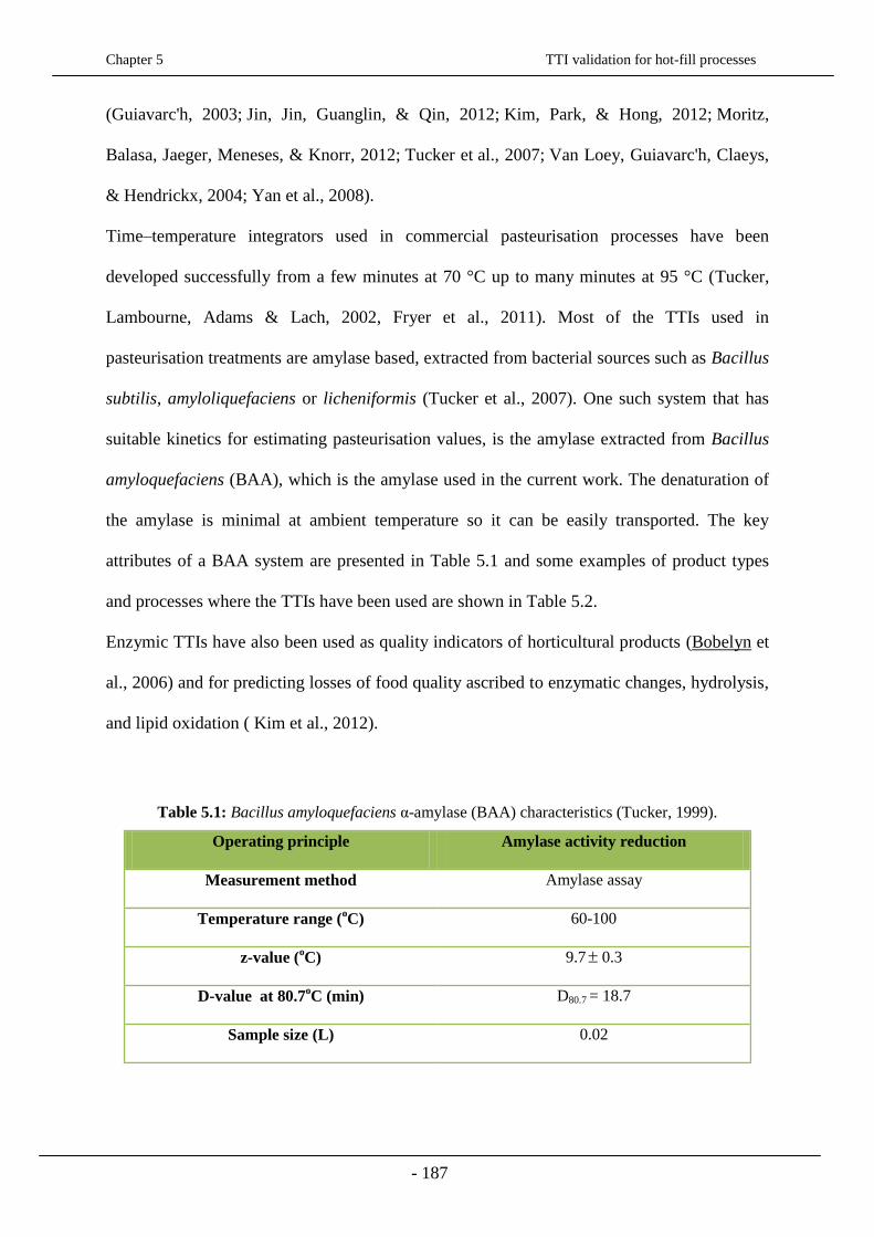
Chapter 5 TTI validation for hot-fill processes
- 187
(Guiavarc'h, 2003; Jin, Jin, Guanglin, & Qin, 2012; Kim, Park, & Hong, 2012; Moritz,
Balasa, Jaeger, Meneses, & Knorr, 2012; Tucker et al., 2007; Van Loey, Guiavarc'h, Claeys,
& Hendrickx, 2004; Yan et al., 2008).
Time–temperature integrators used in commercial pasteurisation processes have been
developed successfully from a few minutes at 70 °C up to many minutes at 95 °C (Tucker,
Lambourne, Adams & Lach, 2002, Fryer et al., 2011). Most of the TTIs used in
pasteurisation treatments are amylase based, extracted from bacterial sources such as Bacillus
subtilis, amyloliquefaciens or licheniformis (Tucker et al., 2007). One such system that has
suitable kinetics for estimating pasteurisation values, is the amylase extracted from Bacillus
amyloquefaciens (BAA), which is the amylase used in the current work. The denaturation of
the amylase is minimal at ambient temperature so it can be easily transported. The key
attributes of a BAA system are presented in Table 5.1 and some examples of product types
and processes where the TTIs have been used are shown in Table 5.2.
Enzymic TTIs have also been used as quality indicators of horticultural products (Bobelyn et
al., 2006) and for predicting losses of food quality ascribed to enzymatic changes, hydrolysis,
and lipid oxidation ( Kim et al., 2012).
Table 5.1: Bacillus amyloquefaciens α-amylase (BAA) characteristics (Tucker, 1999).
Operating principle Amylase activity reduction
Measurement method Amylase assay
Temperature range (oC) 60-100
z-value (oC) 9.7 0.3
D-value at 80.7oC (min) D80.7 = 18.7
Sample size (L) 0.02
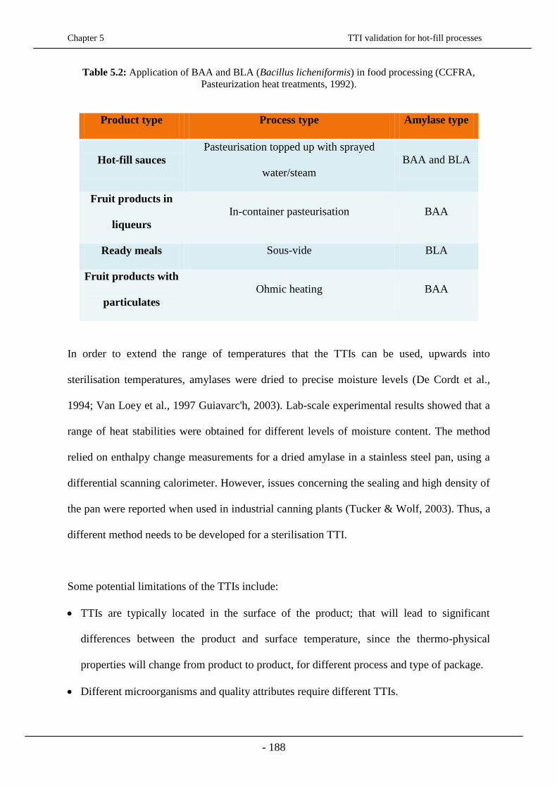
Chapter 5 TTI validation for hot-fill processes
- 188
Table 5.2: Application of BAA and BLA (Bacillus licheniformis) in food processing (CCFRA,
Pasteurization heat treatments, 1992).
In order to extend the range of temperatures that the TTIs can be used, upwards into
sterilisation temperatures, amylases were dried to precise moisture levels (De Cordt et al.,
1994; Van Loey et al., 1997 Guiavarc'h, 2003). Lab-scale experimental results showed that a
range of heat stabilities were obtained for different levels of moisture content. The method
relied on enthalpy change measurements for a dried amylase in a stainless steel pan, using a
differential scanning calorimeter. However, issues concerning the sealing and high density of
the pan were reported when used in industrial canning plants (Tucker & Wolf, 2003). Thus, a
different method needs to be developed for a sterilisation TTI.
Some potential limitations of the TTIs include:
TTIs are typically located in the surface of the product; that will lead to significant
differences between the product and surface temperature, since the thermo-physical
properties will change from product to product, for different process and type of package.
Different microorganisms and quality attributes require different TTIs.
Product type Process type Amylase type
Hot-fill sauces
Pasteurisation topped up with sprayed
water/steam
BAA and BLA
Fruit products in
liqueurs
In-container pasteurisation BAA
Ready meals Sous-vide BLA
Fruit products with
particulates
Ohmic heating BAA
Chapter 5 TTI validation for hot-fill processes
- 189
Extensive experimentation is required for every time the product or the package is altered.
In the current chapter TTIs are tested under the following conditions:
Isothermal: water bath experiments
Calculation of D- and z- value kinetic parameters;
Calculation of process values;
Estimation of TTIs’ heat duration.
Non-isothermal: Peltier Stage experiments
Reliability of TTIs under a variety of time-temperature profiles;
Hot-fill treatment: validation of thermal treatment by comparing TTIs with thermocouples,
submitted under the same conditions.
5.2 Materials and Methods
5.2.1 Preparation of TTIs
TTI solutions are based on commercial α-amylases (powder A6380 Type II A, and liquid
A7595, supplied by Sigma, UK) isolated from Bacillus amyloliquefaciens (BAA). The
amylases denature when heated in buffer solutions and the residual activity, measured using
the Randox colorimetric technique, provides a measure of the thermal process applied to the
food. TTI solutions were formulated by dissolving powder amylase for BAA70, and liquid
amylase for BAA85, in the appropriate buffer systems. Amylase activity was then measured
by using an amylase assay reagent (Randox).
Chapter 5 TTI validation for hot-fill processes
- 190
Preparation of Tris Buffer for BAA85 (0.05 Tris Buffer, pH 8.6 at 25oC)
3.0285 g of Trizma base (Sigma T-6066) (tris hydroxymethyl aminomethane) were weighed
in a 50 mL beaker and dissolved in 500 mL distilled water. The temperature was adjusted to
25oC, using a water bath and the pH was adjusted to 8.5-8.6 using 1 M HCl (Sigma H-7020),
added with a Pasteur pipette (Adams, 1996; Van Loey et al., 1997a). The buffer solution was
kept in the fridge for maximum of one month from its preparation.
Preparation of 10mM acetate buffer for BAA70 (pH 5.0 containing 1mM calcium chloride
(CaCl2.2H2O))
1.36 g of sodium acetate trihydrate were weighed in a 50mL beaker and 40mL of distilled
water were added (100 mM solution). Then 0.036 g of calcium chloride (CaCl2.2H2O) was
weighed into a 50 mL beaker and 25 mL of 100 mM sodium acetate solution were added. The
pH was adjusted to 5.0 using glacial acetic acid.
Bacillus amyloliquefaciens α-amylase at 85°C (BAA85) solution
BAA85 TTI was used for high acid food products in a pH range of 3.7 to 4.2, targeting a process
of 5 minutes at 85°C (CCFRA, 1992a). The solution was prepared by dissolving 50 mg of α-
amylase powder from Bacillus amyloliquefaciens (BAA) in 5 mL of 0.05 M Tris Buffer,
giving a final enzyme concentration of 10 mg/mL.
Bacillus amyloliquefaciens α-amylase at 70°C (BAA70) solution
BAA70 was used for the measurement of mild pasteurisation treatments, targeting a process of
the order of a few minutes at 70°C at the core of the food. The food products that receive these
mild treatments are intended for distribution under refrigerated conditions for up to ten days
storage time, or are naturally high in acid, and are stored under ambient conditions for many
Chapter 5 TTI validation for hot-fill processes
- 191
months. The solution was prepared by dissolving 25 mg of liquid α-amylase in 50 mL of 10
mM Sodium Acetate Buffer at 25oC, giving a final enzyme concentration of 0.5 mg/mL.
Both BAA85 and BAA70 solutions were encapsulated into Altesil (Altec, Cornwall, UK)
high strength silicone tubing with a 2 mm internal bore and 0.5 mm wall thickness cut into
lengths of 15 mm. The two ends of the tube were dipped into silicone elastomer (Sylgard 170,
Dow Corning, USA), heated in a conventional oven at 70oC for the silicone to dry, and then
they were immersed in the buffer solution and stored in the freezer at -18oC.
5.2.1.1 Randox Amylase Calorimetric Method
The Randox amylase test method (Randox Laboratories Ltd) was used to measure the
enzyme activity of both the BAA70 and BAA85 solutions. The method uses
ethylideneblocked p-nitrophenyl-maltoheptaoside as substrate (Substrate 2 from the kit),
which is cleaved by BAA70 and BAA85 into fragments that are further hydrolysed by the
indicator enzyme α-glucosidase, releasing p-nitrophenol and glucose. p-nitrophenol creates a
yellow coloured solution, which can be detected using a spectrophotometer and the rate of
which can be expressed as an activity. The terminal glucose of the substrate is chemically
blocked preventing cleavage by the indicator enzymes (Monza, 2009).
Enzyme Assay procedure
Randox provide a kit containing an amylase substrate and a buffer solution. These kits are
supplied in quantities for 5 assays or 20 assays. Preparation was carried out according to the
manufacturer’s instructions, as follows:
The kit reagents were allowed to equilibrate at room temperature before opening. 20 mL of
Buffer 1 (calcium chloride and sodium chloride) were added to Substrate 2, from the kit. The
amylase solutions of BAA85 and BAA70 were extracted from the TTI silicone tubes using a
Chapter 5 TTI validation for hot-fill processes
- 192
syringe. 10 μL of BAA85 solution were diluted with 290 μL of 50 mM Tris Buffer (30-fold
dilution), while 15 μL of BAA70 were diluted with 15 μL of 10 mM Acetate Buffer (2-fold
dilution). 20 μL of each diluted solution was added to a cuvette containing 1 mL of the
enzyme essay reagent from Randox (Crumlin, UK). The cuvette was then immediately placed
into the chamber of the spectrophotometer (CECIL, Cambridge, UK) and the absorbance, at a
wavelength of 405 nm and 30°C, was measured. The readings from the spectrophotometer
were taken over a 5 minute period.
5.2.1.2 Determination of BAA70 and BAA85 activity
According to the above, the reaction rate of both solutions can be determined by plotting the
absorbance readings of BAA70 and BAA85 against time.
Highly active solutions, such as the control samples, reached a constant gradient soon after
starting the assay, whereas samples with low enzyme activity required more time. The
amylase activities were calculated based on the gradient with the fastest reaction rate of
absorbance with time. Figure 5.1 illustrates the reaction rate curve for a control (unheated)
amylase, sample of BAA70, prepared according to § 5.2.1, in which the initial rate rA is
0.014s-1
, based on equation 5.1:
BAAfA Ckr (5.1)
Where: rA is the reaction rate, kf is the first order rate constant and CBAA is the active BAA
concentration.
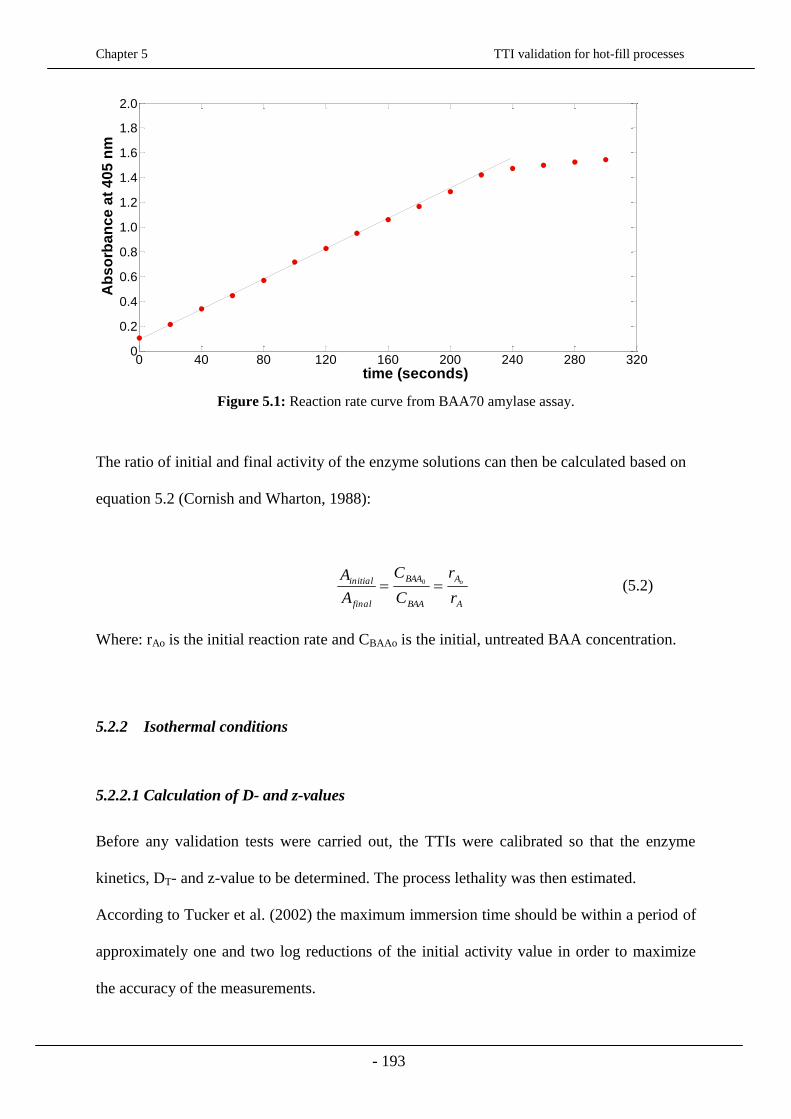
Chapter 5 TTI validation for hot-fill processes
- 193
0 40 80 120 160 200 240 280 3200
0.2
0.4
0.6
0.8
1.0
1.2
1.4
1.6
1.8
2.0
time (seconds)
Ab
so
rba
nc
e a
t 4
05
nm
Figure 5.1: Reaction rate curve from BAA70 amylase assay.
The ratio of initial and final activity of the enzyme solutions can then be calculated based on
equation 5.2 (Cornish and Wharton, 1988):
A
A
BAA
BAA
final
initial
r
r
C
C
A
Ao 0 (5.2)
Where: rAo is the initial reaction rate and CBAAo is the initial, untreated BAA concentration.
5.2.2 Isothermal conditions
5.2.2.1 Calculation of D- and z-values
Before any validation tests were carried out, the TTIs were calibrated so that the enzyme
kinetics, DT- and z-value to be determined. The process lethality was then estimated.
According to Tucker et al. (2002) the maximum immersion time should be within a period of
approximately one and two log reductions of the initial activity value in order to maximize
the accuracy of the measurements.
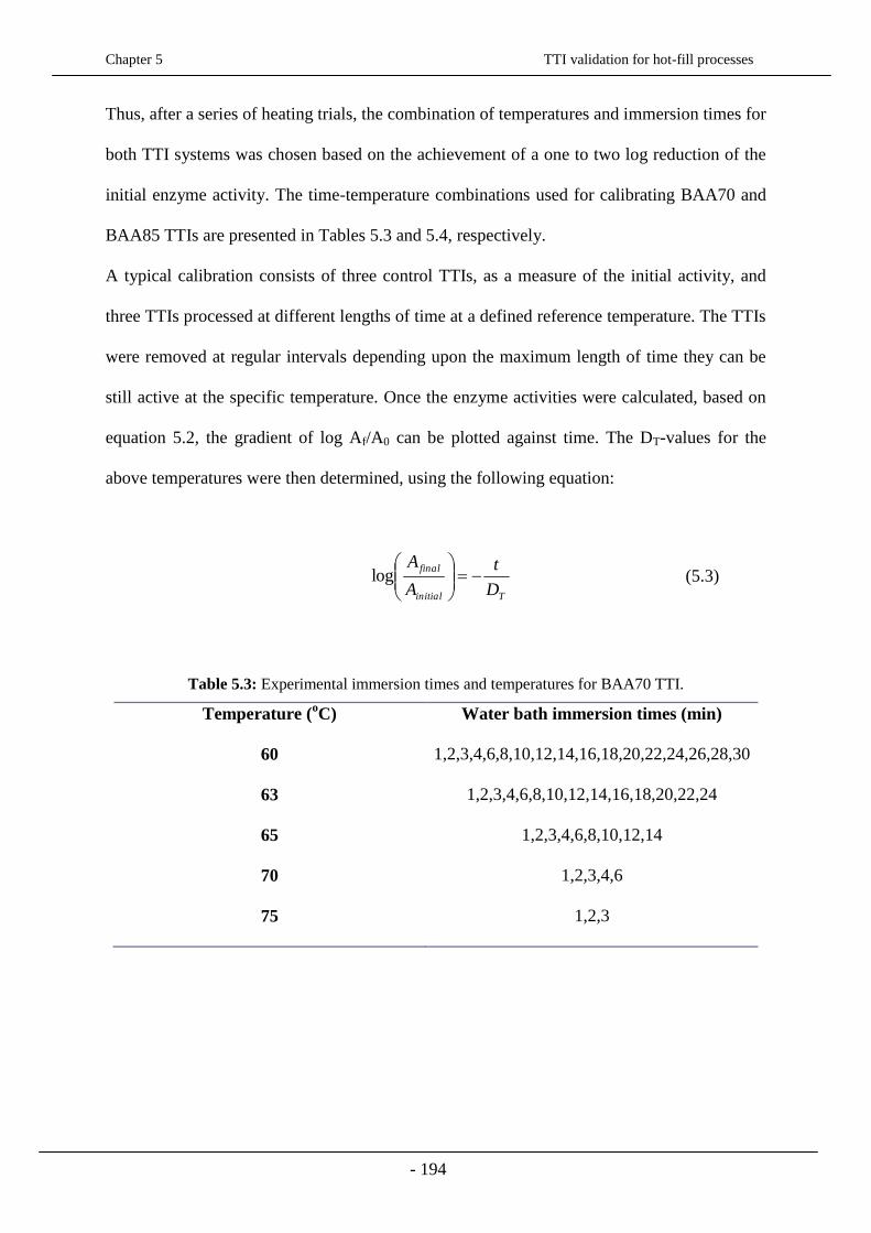
Chapter 5 TTI validation for hot-fill processes
- 194
Thus, after a series of heating trials, the combination of temperatures and immersion times for
both TTI systems was chosen based on the achievement of a one to two log reduction of the
initial enzyme activity. The time-temperature combinations used for calibrating BAA70 and
BAA85 TTIs are presented in Tables 5.3 and 5.4, respectively.
A typical calibration consists of three control TTIs, as a measure of the initial activity, and
three TTIs processed at different lengths of time at a defined reference temperature. The TTIs
were removed at regular intervals depending upon the maximum length of time they can be
still active at the specific temperature. Once the enzyme activities were calculated, based on
equation 5.2, the gradient of log Af/A0 can be plotted against time. The DT-values for the
above temperatures were then determined, using the following equation:
Tinitial
final
D
t
A
A
log (5.3)
Table 5.3: Experimental immersion times and temperatures for BAA70 TTI.
Temperature (oC) Water bath immersion times (min)
60 1,2,3,4,6,8,10,12,14,16,18,20,22,24,26,28,30
63
65
1,2,3,4,6,8,10,12,14,16,18,20,22,24
1,2,3,4,6,8,10,12,14
70 1,2,3,4,6
75 1,2,3
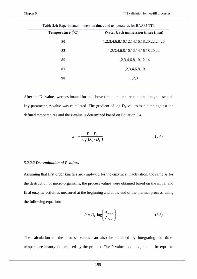
Chapter 5 TTI validation for hot-fill processes
- 195
Table 5.4: Experimental immersion times and temperatures for BAA85 TTI.
Temperature (oC) Water bath immersion times (min)
80 1,2,3,4,6,8,10,12,14,16,18,20,22,24,26
83
85
1,2,3,4,6,8,10,12,14,16,18,20,22
1,2,3,4,6,8,10,12,14
87 1,2,3,4,6,8,10
90 1,2,3
After the DT-values were estimated for the above time-temperature combinations, the second
key parameter, z-value was calculated. The gradient of log DT-values is plotted against the
defined temperatures and the z-value is determined based on Equation 5.4:
12
/log
21
TT DD
TTz
(5.4)
5.2.2.2 Determination of P-values
Assuming that first order kinetics are employed for the enzymes’ inactivation, the same as for
the destruction of micro-organisms, the process values were obtained based on the initial and
final enzyme activities measured at the beginning and at the end of the thermal process, using
the following equation:
final
initialT
A
ADP log.
(5.5)
The calculation of the process values can also be obtained by integrating the time-
temperature history experienced by the product. The P-values obtained, should be equal to
Chapter 5 TTI validation for hot-fill processes
- 196
the ones calculated from the TTIs, provided that the assumption of first order kinetics holds
for the enzymes over the whole temperature range they have experienced. The combination
of the two monitoring techniques used to validate the thermal process is expressed as follows:
final
initialT
t
z
TreftT
A
ADdtP log.10 .
0
)(
(5.6)
Tref equals the value of 85oC and 70
oC, for BAA70 and BAA85, respectively, with the
appropriate, estimated z-values.
5.2.3 Non-isothermal conditions: Peltier stage
The TTIs were tested under non-isothermal conditions for their sensitivity to be evaluated at
various time-temperature profiles. A Peltier stage (Linkam, Tadworth, UK), was used to
provide the time temperature profiles by control of the applied voltage to its thermoelectric
module – the Peltier and its operational principle are illustrated in Figure 5.2.
The thermoelectric module was connected to a water circulating pump (ECP 220-240V/50
Hz, Linkam, Tadworth, UK) that keeps the device from overheating and being damaged, and
a computer, where the time-temperature profiles were set and controlled. The software used
was Linksys 32 (Linkam, Tadworth, UK).

Chapter 5 TTI validation for hot-fill processes
- 197
Figure 5.2: Experimental configuration of Peltier stage (top), Linkam Peltier module used and its
principle of operation (bottom) (http://www.huimao.com/).
The reliability of the Peltier system was checked by attaching a thermocouple on the
thermoelectric module using adhesive tape. The time-temperature history recorded from the
thermocouple data logger was compared to that obtained from the internal temperature
measurement from the Peltier stage.
In order to test the sensitivity of the TTIs on temperature changes, three TTIs and one more
with a calibrated thermocouple (type K) inside, were attached to the thermoelectric module,
Peltier stage
Data Logger

Chapter 5 TTI validation for hot-fill processes
- 198
using a heat sink compound (RS, Corby, UK, thermal conductivity = 0.9 (W m-1
K-1
) that
ensured good thermal contact between them and the Peltier plate. The enzyme activities
obtained from the TTIs were compared to the time-temperature history recorded from the
thermocouple inside the fourth TTI, in terms of process values, using equation 5.6. The above
non-isothermal conditions were repeated five times.
The experiments conducted on the Peltier stage, were separated into two different sets:
5.2.3.1 Simple cycles
The heating and cooling rate of the process is kept constant, and the holding time is of great
importance, as it is the factor that affects the lethality of the process the most. Such a process
is usually batch, where a retort is used for the heating, holding and cooling phases of the
treatment. The calculation of lethality in these types of processes is easier as compared to
variable time-temperature conditions. The evaluation of thermal processes at a constant lethal
temperature is relatively easy; but the temperature throughout a process is rarely constant.
The TTIs were heated up at two different reference temperatures, 70 and 85oC, at a constant
heating/cooling rate of 30°C min-1
. The holding time at which the TTIs and the
thermocouples were kept, for the above two Tref, varied from 2 to 10 min. The TTIs were
then cooled down to 20°C, at the same rate of 30°C min-1
. The holding time, the number of
repetitions for each Tref and the number of TTIs and thermocouples used on the plate are
shown in Table 5.5.

Chapter 5 TTI validation for hot-fill processes
- 199
Table 5.5: Experiments conducted on Peltier stage at constant heating/cooling rate.
Holding time
(min) at Tref=70oC
(BAA70)
Holding time
(min) at Tref=85oC
(BAA85)
Repetitions
Number of
TTIs
Number of
thermocouples
1 2 5 15 10
2 4 5 15 10
3 6 5 15 10
4 8 7 21 14
6 10 7 21 14
8 12 7 21 14
5.2.3.2 Complex cycles
The second set of experiments refers to complex time-temperature profiles which are more
relevant to industrial continuous processes, such as hot-fill treatments; the product is
continuously processed usually into tunnels with the sections of heating, holding, and
cooling. The TTIs were heated up at two different rates, 15 and 30°C min-1
, until the
reference temperature of 70 or 85°C was reached, with no holding time, and were
immediately cooled down to 20°C, at the same rates. The repetitions and number of TTIs and
thermocouples used are summarised in Table 5.6.

Chapter 5 TTI validation for hot-fill processes
- 200
Table 5.6: Complex cycles produced on Peltier stage for a heating/cooling rate of
15 and 30°C min-1
.
Holding time
(min)
Tref (oC)
Repetition of t-
T profiles
Repetitions
Number of
TTIs
Number of
thermocouples
0 70/85 x1 5 15 10
0 70/85 x2 5 15 10
0 70/85 x3 5 15 10
0 70/85 x4 5 15 10
For both simple and complex cycle, the standard deviation between the repetitions resulted in
a value lower than 3. Thus, the average values were taken as representative for illustrating the
data obtained in Figures 5.6-5.9.
5.3 Results and Discussion
5.3.1 Isothermal conditions: kinetic parameters and heat treatment duration
The log of initial (Ao) /final (A) amylase activity was plotted against a defined heating time
for both BAA70 and BAA85 as illustrated in Figure 5.3. The values of D70°C and D85°C were
then calculated based on equation 5.3 and are presented in Table 5.7.

Chapter 5 TTI validation for hot-fill processes
- 201
Figure 5.3: The BAA70 and BAA85 DT-value calculation curves.
Table 5.7: Calculated DT-values for BAA70 and BAA85 solutions.
Test temperature (°C) DT-value (min) Test temperature (°C) DT-value (min)
BAA70 BAA85
60 40.8 80 25.0
63 18.3 83 16.6
65 7.3 85 8.7
70 4.1 87 6.6
75 1.6 90 2.7
The log of the above determined DT-values was then plotted against temperature, Figure 5.4,
for both solutions and the z-values were calculated based on equation 5.5.

Chapter 5 TTI validation for hot-fill processes
- 202
Figure 5.4: The BAA70 and BAA85 z-value curve.
A D70°C-value of 4.1±0.4 min was obtained for BAA70 at Tref=70oC, which is significantly
low in comparison to the value of 8.4 min reported in literature (Lambourne and Tucker,
2001). That is probably due to the different amylase batches being used and/or the storage
conditions of the TTIs. The z-value of BAA70 was calculated to be 10.8±0.5oC, which is
within the range of the values used for the evaluation of safety of the pasteurisation processes
for several microorganisms with z-values from 5 to 12oC (Van Loey et al., 1997).
The D85°C-value for BAA85 was calculated to be 8.7±0.3 min, higher than the value of 6.8
min found by Lambourne and Tucker, (2001). That is possibly owing to the different α-
amylase used in the current project. The liquid form of amylase used, shows optimal activity
at the range between 70oC and 90
oC, in comparison to the powder amylase used in
experimental work reported from literature (Hendrickx et al., 1992), where the amylase
shows an optimum at 65oC. The higher DT-value obtained from the liquid amylase, indicates
that the specific amylase is more heat resistant than the powder one, and would possibly be
more accurate in monitoring higher temperatures in pasteurisation treatments. The z-value of

Chapter 5 TTI validation for hot-fill processes
- 203
BAA85 was 10.3±0.3°C, consistent with the values used for monitoring pasteurization
processes. The kinetic parameters obtained from the experimental work are shown as
compared to the values reported in literature, in Table 5.8.
In order for the TTIs to accurately represent the effect of a thermal treatment on
microorganisms of interest, it is important that their kinetics resemble that of the target
organism, which would result in similar lethality. Thus, TTIs could accurately mimic the
destruction rate of microorganisms and be used safely in validating thermal processes.
Table 5.8: α-amylase TTIs used in pasteurisation treatments of foods
(CCFRA guidelines, 2006b).
In the current work, the denaturation of Bacillus amyloliquefaciens α-amylase was used as
the TTI system that can be used in pasteurisation treatments (60–105°C). The kinetics
obtained under non-isothermal conditions was proved to be reliable for its use in measuring
integrated process values (Van Loey and Arthawan, 1997a).
The z-values of both BAA70 and BAA85 enzymes appear to be higher than those of the
targeted processes, which is in agreement with what is found in literature about enzymes
Product pH Target
microorganisms Target process
DT-value
(min)
z-value
(oC)
DT-value
(min)
z-value
(oC)
Literature Experimental
Cook-chill
<3.5
Acid-philic yeasts and
moulds, and
lactobacilli
2 min at 70oC
BAA70 8-10 8-9 4.1±0.4 10.8±0.5
High acid
3.5-4.0
Acid tolerant yeasts
and moulds, spore-
forming bacteria
5 min at 85oC
BAA85 8-10 9-9.5 8.7±0.3 10.3±0.3
Sous-vide
4.0-4.2 spore-forming bacteria
10 min at 90oC
BLA90 15-25 9-9.5 -
Acid
4.2-4.5 spore-forming bacteria
5 or 10 min at
93.3oC
BLA93
8-12 9-9.5 -

Chapter 5 TTI validation for hot-fill processes
- 204
implicated in mild thermal processes concerning acid and high-acid food products
(Hendrickx et al., 1996). Hence, if the process values of the enzymes are used to predict the
actual values of the thermal treatment, the filling temperature needs to be larger than the
reference temperature, so that the target process value to be achieved. As far as the heat
duration of the TTIs is concerned, the chosen immersion times resulted in one to two log
reductions of activity for both enzymatic solutions, maximizing the accuracy of the
measurements (Tucker et al., 2002). Consequently, TTIs should be able to endure heat
treatments for maximum 2DT-values. According to the kinetics obtained, the BAA70 and
BAA85 solutions should be accurately used for heat duration of maximum 8.2 min and 17.4
min, respectively.
The calculation of the process values was based on equation 5.3. The obtained values were
plotted against the defined immersion times, in order to estimate the heat duration of the two
TTI systems. Figure 5.5 illustrates the correlation of the TTIs with the processing time using
the ideal Y=X curve; R2 was calculated to be 0.993 and 0.995 for BAA70 and BAA85
respectively. According to Figure 5.5, the maximum heat duration of BAA70 is 7 min, and
that of BAA85 is 16 min, which are slightly lower than the ones expected to be achieved,
according to the 2DT-value theory. The fact that the BAA70 has a shorter shelf life than
BAA85 is possibly owing to the significant difference in their DT-values, D70-value is half of
D85, indicating that BAA70 is less temperature resistant than BAA85.
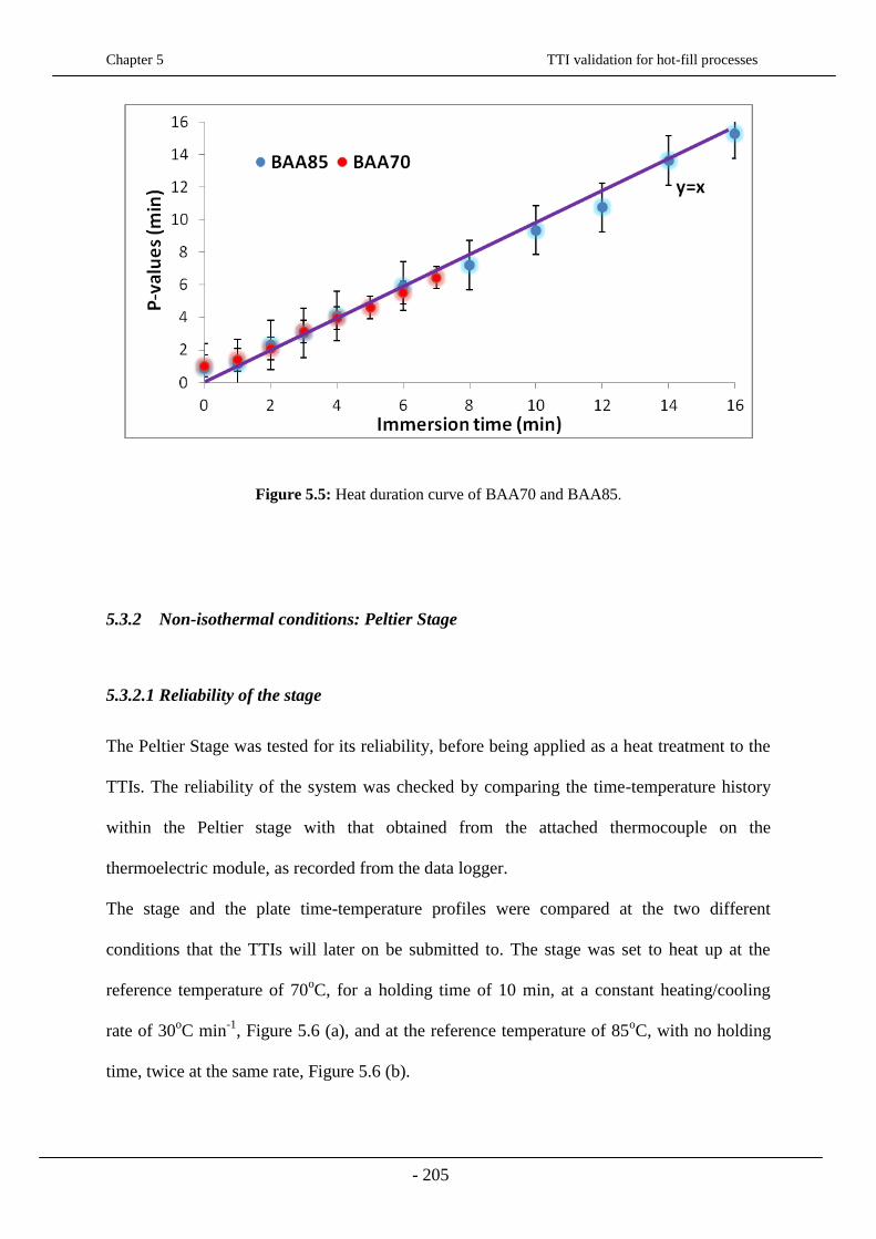
Chapter 5 TTI validation for hot-fill processes
- 205
Figure 5.5: Heat duration curve of BAA70 and BAA85.
5.3.2 Non-isothermal conditions: Peltier Stage
5.3.2.1 Reliability of the stage
The Peltier Stage was tested for its reliability, before being applied as a heat treatment to the
TTIs. The reliability of the system was checked by comparing the time-temperature history
within the Peltier stage with that obtained from the attached thermocouple on the
thermoelectric module, as recorded from the data logger.
The stage and the plate time-temperature profiles were compared at the two different
conditions that the TTIs will later on be submitted to. The stage was set to heat up at the
reference temperature of 70oC, for a holding time of 10 min, at a constant heating/cooling
rate of 30oC min
-1, Figure 5.6 (a), and at the reference temperature of 85
oC, with no holding
time, twice at the same rate, Figure 5.6 (b).

Chapter 5 TTI validation for hot-fill processes
- 206
0 200 400 600 80025
35
45
55
65
75
Time (sec)
Tem
pera
ture
(oC
) BAA70 at Tref=70oC
0 100 200 300 400 50025
35
45
55
65
75
85
90
Time (sec)T
em
pera
ture
(oC
)
BAA85 at
Tref=85oC
stage plate
stage plate
a. b.
Figure 5.6: Time-temperature profiles of the Peltier stage and the thermoelectric module for a.
BAA70 and b. BAA85.
It appears that the temperatures recorded on the plate, are very consistent with the ones
obtained from the stage, in both conditions, making the method reliable for testing the TTIs’
sensitivity under tightly controlled time-temperature conditions. The slight difference of 0.5-
1oC is possibly due to measurement sampling rate; the stage temperature is recorded every
0.30 seconds, whilst the one of the thermocouple is recorded every second. Another reason
can be the thermocouples moving during the treatment.
After the accuracy of the Peltier stage was confirmed, three TTIs plus one with a
thermocouple inside were attached to the thermoelectric module. The thermocouple was
inserted in the TTI in order to test whether the process values obtained from the amylase
reduction are consistent with the values obtained from the time-temperature profile that the
thermocouple records inside the TTI. That way, the TTIs can be comparable with the time
temperature recorded on the thermoelectric module, since the TTIs cannot record the changes
in a continuous process; they would have to be removed and measured in every step of the
Chapter 5 TTI validation for hot-fill processes
- 207
heat treatment applied. The Peltier stage was set to heat up at the reference temperatures of
70oC for a range of holding times from 2 to 10 min for BAA70, and at a reference
temperature of 85oC, with no holding time, repeated twice in a consequent cycle. The time-
temperature profiles were recorded until both TTI systems reached the temperature of 70oC,
at a rate of 30oC min
-1; the experiments were repeated 5 times for both TTI solutions. The
time-temperature profile obtained from the thermocouples and the enzyme activities
measured at the beginning and the end of the process were compared in terms of process
values, based on Equation 5.6; the process values shown in Figure 5.7 are the average values
obtained from the 5 replications, for all the time-temperature histories applied on the module.
The linear fit curve indicated a very good agreement between the two process-value sets; the
observation was confirmed by the calculated standard deviation values of 0.024 and 0.014
min for BAA70 and BAA85, respectively.
The results indicate that recording the time-temperature profile of the amylase by the inserted
thermocouple, instead of measuring its activity, is reliable. Thus, the heating/cooling profiles
applied by the stage, will make the comparison of TTIs and thermocouples placed on the
module more convenient.

Chapter 5 TTI validation for hot-fill processes
- 208
Figure 5.7: Correlation between the temperatures recorded from the thermocouple inside the TTIs,
and the enzyme activity of the TTIs.
5.3.2.2 Simple cycles
The Peltier stage was set to heat up the module until the reference temperatures of 70, 85 and
90oC were reached. The holding time was set from 2 to 12 min, for all three reference
temperatures and the cooling cycle was set to reach 20°C; the heating/cooling rate was kept
constant at 30°C min-1
. The different reference temperatures and holding times were chosen
in order to test the sensitivity of the TTIs under a variety of conditions.
Three BAA70 and BAA85 TTIs were attached to the thermoelectric module, with inserted
thermocouples; an extra thermocouple also used, which was in direct contact with the
module; the time-temperature profiles of the two monitoring techniques were recorded by the
Peltier stage and were compared.
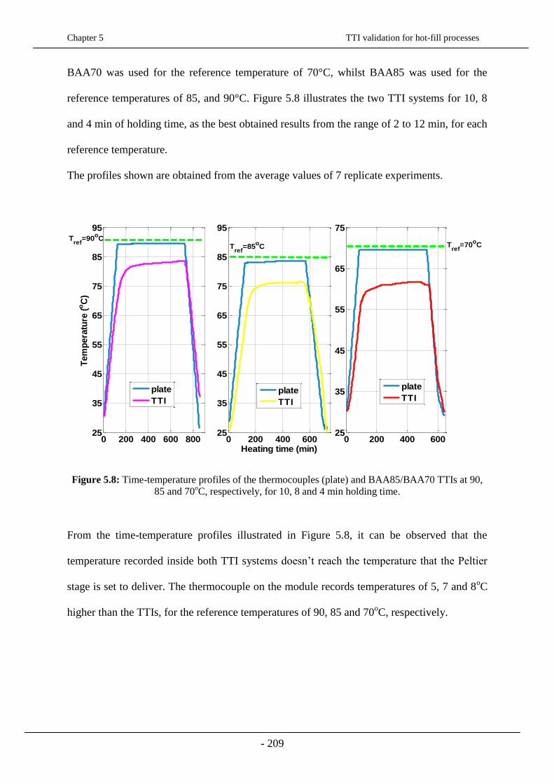
Chapter 5 TTI validation for hot-fill processes
- 209
BAA70 was used for the reference temperature of 70°C, whilst BAA85 was used for the
reference temperatures of 85, and 90°C. Figure 5.8 illustrates the two TTI systems for 10, 8
and 4 min of holding time, as the best obtained results from the range of 2 to 12 min, for each
reference temperature.
The profiles shown are obtained from the average values of 7 replicate experiments.
0 200 400 600 80025
35
45
55
65
75
85
95
Tem
pera
ture
(oC
)
0 200 400 60025
35
45
55
65
75
85
95
Heating time (min)
0 200 400 60025
35
45
55
65
75
plate
TTI
plate
TTIplate
TTI
Tref
=70oCT
ref=85
oC
Tref
=90oC
Figure 5.8: Time-temperature profiles of the thermocouples (plate) and BAA85/BAA70 TTIs at 90,
85 and 70oC, respectively, for 10, 8 and 4 min holding time.
From the time-temperature profiles illustrated in Figure 5.8, it can be observed that the
temperature recorded inside both TTI systems doesn’t reach the temperature that the Peltier
stage is set to deliver. The thermocouple on the module records temperatures of 5, 7 and 8oC
higher than the TTIs, for the reference temperatures of 90, 85 and 70oC, respectively.

Chapter 5 TTI validation for hot-fill processes
- 210
Reasons for that can be:
The thickness of the silicone tube used, which can give rise to larger heating lags;
The faster heat received by the thermocouples (prone to conduction), due to their higher
thermal conductivity and small size;
Experimental error: non-proper application of the heat sink compound on the TTIs, the
thermocouples moving during the process.
5.3.2.3 Complex cycles
The second set of experiments refers to complex time-temperature profiles that are more
relevant to industrial, continuous thermal processes. The TTIs were heated up at a rate of
30°C min-1
, until the reference temperature of 70, 85 and 90°C was reached. No holding time
was set and the solutions were immediately cooled down to 30°C, at the same rate. The cycle
was repeated for 1 to 4 times for both enzymes. The repetitions and number of TTIs and
thermocouples used are summarised in Table 5.5. The cycles chosen to be illustrated as the
best obtained result for BAA70 TTI, at a reference temperature of 70°C, were four
consequent heating/cooling cycles, three for 85°C and 2 for 90°C, referring to BAA85 TTI.
Similarly to the simple cycles, three BAA70 and BAA85 TTIs were attached to the
thermoelectric module, with inserted thermocouples and an extra thermocouple in direct
contact with the module. The time-temperature profiles of the two monitoring techniques
were recorded by the Peltier stage and were compared under a variety of complex conditions
for testing the sensitivity of the TTIs.

Chapter 5 TTI validation for hot-fill processes
- 211
0 200 40025
35
45
55
65
75
85
95
Tem
pera
ture
(oC
)
0 200 400 600 80025
35
45
55
65
75
85
95
Heating time (min)
0 200 400 60025
35
45
55
65
75
plate TTIplate TTIplate TTI
Tref
=85oC
Tref
=90oC
Tref
=70oC
Figure 5.9: Complex time-temperature profiles of the thermocouples (plate), BAA85 and BAA70
TTIs at 90 oC (2 heating/cooling cycles), 85
oC (3 heating/cooling cycles), and 70
oC, (4
heating/cooling cycles), respectively.
The temperature recorded at the core of the TTIs indicates that the enzymic solutions are able
to pick up small temperature changes throughout the process, but are not sensitive enough to
reach the temperature that the thermocouples record on the module. Similarly as with the
simple cycles, the higher the reference temperature, the lower the temperature difference
between the TTI systems and the thermocouples is; a difference of 5, 7 and 8oC, is observed
for the reference temperatures of 90, 85 and 70oC, respectively.
The above observations are reflected in Figure 5.9, where the process values of the
thermocouples attached on the thermoelectric module are plotted against those obtained from
the TTIs under both the simple and complex heating/cooling conditions defined earlier. The
time-temperature history illustrated in Figures 5.8 and 5.9 is integrated and converted into
process values based on the left part of Equation 5.6.
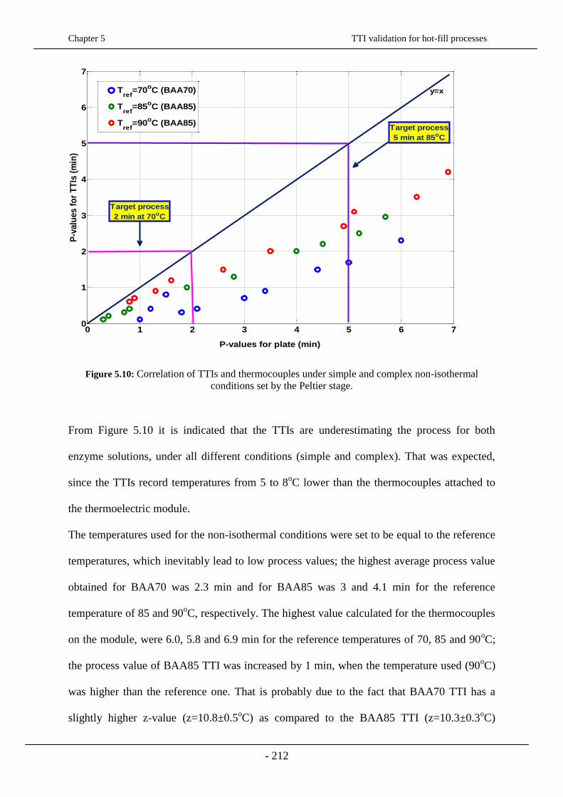
Chapter 5 TTI validation for hot-fill processes
- 212
0 1 2 3 4 5 6 70
1
2
3
4
5
6
7
P-values for plate (min)
P-v
alu
es f
or
TT
Is (
min
)
Tref
=70oC (BAA70)
Tref
=85oC (BAA85)
Tref
=90oC (BAA85)
y=x
Target process
2 min at 70oC
Target process
5 min at 85oC
Figure 5.10: Correlation of TTIs and thermocouples under simple and complex non-isothermal
conditions set by the Peltier stage.
From Figure 5.10 it is indicated that the TTIs are underestimating the process for both
enzyme solutions, under all different conditions (simple and complex). That was expected,
since the TTIs record temperatures from 5 to 8oC lower than the thermocouples attached to
the thermoelectric module.
The temperatures used for the non-isothermal conditions were set to be equal to the reference
temperatures, which inevitably lead to low process values; the highest average process value
obtained for BAA70 was 2.3 min and for BAA85 was 3 and 4.1 min for the reference
temperature of 85 and 90oC, respectively. The highest value calculated for the thermocouples
on the module, were 6.0, 5.8 and 6.9 min for the reference temperatures of 70, 85 and 90oC;
the process value of BAA85 TTI was increased by 1 min, when the temperature used (90oC)
was higher than the reference one. That is probably due to the fact that BAA70 TTI has a
slightly higher z-value (z=10.8±0.5oC) as compared to the BAA85 TTI (z=10.3±0.3
oC)
Chapter 5 TTI validation for hot-fill processes
- 213
leading to a higher process value and consequently smaller temperature difference with the
thermocouples on the plate.
The BAA85 TTIs do not reach the target process for neither of the reference temperatures,
whilst the BAA70 TTIs reached the target of 2 min under the simple cycle conditions applied
for a holding time ≥4 min. Thus, the TTI systems are not appropriate for assessing hot-fill
treatments, under the specific time-temperature conditions. In order to avoid the need for top-
up pasteurisation they need to be tested under conditions where the temperatures used, will be
higher than the reference ones. In the following section, the TTIs are submitted to conditions
more industrially realistic.
5.3.3 Hot-filling by the method of inversion
In the third set of experiments conducted, the TTIs are being tested under the non-isothermal
conditions of the hot-fill treatment, described in Chapter 2.
Based on the above derived conclusions, from the sensitivity tests conducted, it appeared that
the TTI systems cannot reach the temperature applied to them by the thermoelectric module
and they record lower temperatures than the thermocouples attached on the same plate, when
the temperatures applied are equal or close to the reference temperatures. Thus, in order to
overcome that problem, in the hot-fill treatments in which the TTI solutions were subjected,
the filling temperatures were higher than the reference ones, for the TTIs to be possibly more
comparable with the thermocouples, subjected under the same conditions.
The TTIs and the thermocouples were positioned in places of interest, where the cold spots
are likely to be, on the inside of a glass jar, as illustrated in Figure 5.11. Positions 1, 2, 3, 4
and 5 refer to the bottom, bottom-corner, wall, headspace and the lid, respectively.

Chapter 5 TTI validation for hot-fill processes
- 214
Figure 5.11: Location of TTIs and thermocouples in a glass jar.
The hot-fill treatment experiments were conducted for three different fluids: water, 3% of
starch solution (w/w) and cream of tomato soup. The choice was made based on the different
thermal properties of the fluids in order to test the response of the TTIs under a variety of
fluid conditions. The thermal properties of the fluids were calculated based on Equations 3.4-
3.8, Chapter 3, §3.2.3.1, and are presented in Table 5.9.
Table 5.9: Properties of the fluids used at 70oC.
k (W m-1
K-1
) Cp (kJ kg-1
K-1
) ρ (kg m-3
) η (Pa s)
at γ=10 s-1
water 0.590 4.181 998.2 0.001
3% starch 0.313 4.011 1026 0.30
Tomato soup 0.315 3.673 1050 1.30
1
3
2
5
4

Chapter 5 TTI validation for hot-fill processes
- 215
The fluids were chosen to be pasteurised at 75 and 90oC for BAA70 and BAA85,
respectively. The reasons for the specific filling temperatures were:
The need for higher temperatures than the reference ones, for minimising the tendency of
the TTIs to underestimate the process, as explained above, and
The heat duration of the TTI systems (BAA70 at 70oC = 7 min and BAA85 at 85
oC = 16
min); the enzyme activity recorded within 5oC, for both enzymes didn’t affect
significantly the process values obtained. For a process time of 10 min, at the above
chosen temperatures, the TTIs could endure the heat treatment and be more comparable to
the thermocouples.
After being pasteurised, the fluids were filled into a glass jar, which was sealed and air-
cooled for approximately 10 min.
The jars were preheated before being hot-filled, at the same temperature the fluids were
pasteurised, in order to minimise any heat losses that can occur between the times the fluid is
hot-filled and the jar is sealed, and to avoid a possible thermal shock of the package.
The obtained enzyme activity of the TTIs and the time-temperature history of the
thermocouples were converted into process values, based on Equation 5.6, and were then
compared for both target processes of 2 min at 70oC and 5 min at 85
oC.
Figures 5.12 and 5.13 compare the process values of the thermocouples and TTIs at a filling
temperature of 75oC and 90
oC for BAA70 and BAA85, respectively at all the locations of
interest.
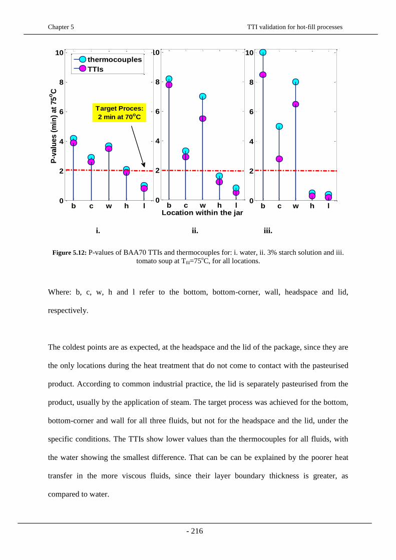
Chapter 5 TTI validation for hot-fill processes
- 216
b c w h l0
2
4
6
8
10
Location within the jar
b c w h l0
2
4
6
8
10
b c w h l0
2
4
6
8
10P
-valu
es (
min
) at
75
oC
thermocouples
TTIs
Target Proces:
2 min at 70oC
i. ii. iii.
Figure 5.12: P-values of BAA70 TTIs and thermocouples for: i. water, ii. 3% starch solution and iii.
tomato soup at Tfil=75oC, for all locations.
Where: b, c, w, h and l refer to the bottom, bottom-corner, wall, headspace and lid,
respectively.
The coldest points are as expected, at the headspace and the lid of the package, since they are
the only locations during the heat treatment that do not come to contact with the pasteurised
product. According to common industrial practice, the lid is separately pasteurised from the
product, usually by the application of steam. The target process was achieved for the bottom,
bottom-corner and wall for all three fluids, but not for the headspace and the lid, under the
specific conditions. The TTIs show lower values than the thermocouples for all fluids, with
the water showing the smallest difference. That can be can be explained by the poorer heat
transfer in the more viscous fluids, since their layer boundary thickness is greater, as
compared to water.
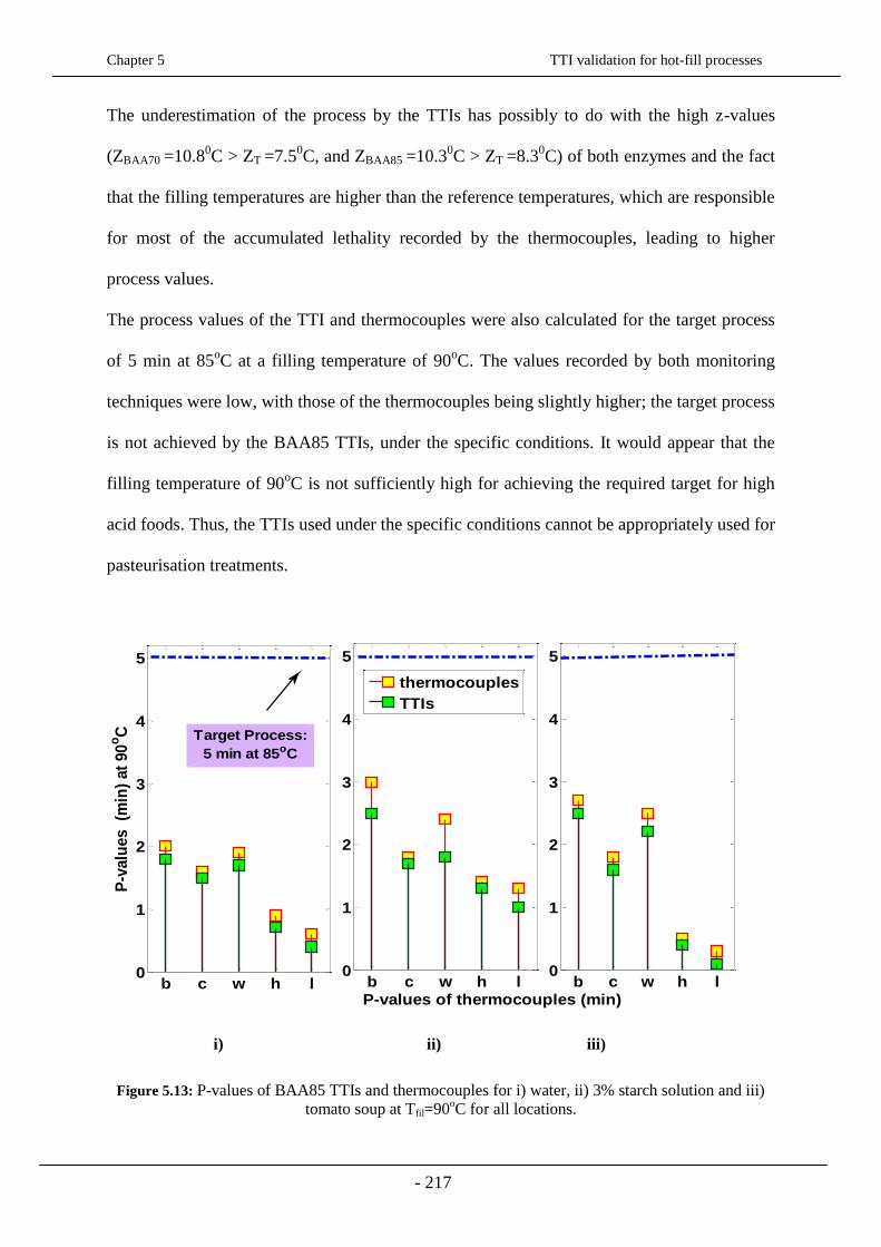
Chapter 5 TTI validation for hot-fill processes
- 217
The underestimation of the process by the TTIs has possibly to do with the high z-values
(ZBAA70 =10.80C > ZT =7.5
0C, and ZBAA85 =10.3
0C > ZT =8.3
0C) of both enzymes and the fact
that the filling temperatures are higher than the reference temperatures, which are responsible
for most of the accumulated lethality recorded by the thermocouples, leading to higher
process values.
The process values of the TTI and thermocouples were also calculated for the target process
of 5 min at 85oC at a filling temperature of 90
oC. The values recorded by both monitoring
techniques were low, with those of the thermocouples being slightly higher; the target process
is not achieved by the BAA85 TTIs, under the specific conditions. It would appear that the
filling temperature of 90oC is not sufficiently high for achieving the required target for high
acid foods. Thus, the TTIs used under the specific conditions cannot be appropriately used for
pasteurisation treatments.
b c w h l0
1
2
3
4
5
b c w h l0
1
2
3
4
5
thermocouples
TTIs
b c w h l0
1
2
3
4
5
P-values of thermocouples (min)
P-v
alu
es
(min
) at
90
oC
Target Process:
5 min at 85oC
i) ii) iii)
Figure 5.13: P-values of BAA85 TTIs and thermocouples for i) water, ii) 3% starch solution and iii)
tomato soup at Tfil=90oC for all locations.

Chapter 5 TTI validation for hot-fill processes
- 218
In both target processes the filling temperature is higher than the reference temperature and
the z-values are higher than the ones of the target processes leading to underestimation of the
process, which confirms the results reported in literature (Van Loey et al., 1996), as presented
in Table 5.10.
Table 5.10: Possible scenarios for hot-fill processes.
Tfil > Tref Tfil < Tref
ZTTI > ZT Underestimation Overestimation
ZTTI < ZT Overestimation Underestimation
Where: Tfil = filling temperature, Tref = reference temperature, ZTTI = z-value of the enzyme,
ZT = z-value of the target process.
According to Table 5.10, The TTIs would overestimate the process at temperatures lower
than the reference temperatures, as the lethality at temperatures lower than 60 and 750C, for
BAA70 and BAA85, respectively, is negligible. Thus, the thermocouples would record much
lower temperatures than the TTIs, which would overestimate that way the process, for the
given z-values. This scenario would be the worse in terms of safety.
The measurement limit of the spectrophotometer was three log reductions in amylase activity
with a reading to 3 decimal points. An average initial amylase activity for the BAA85 TTI
and BAA70 was 1.000 and 0.9 units/minute, which for 3 log reductions would result in 0.001
units/minute activity for both TTI solutions. The highest process-values calculated from the
amylase activities were ≤ 0.002 min-1
, which was the limit of the measuring accuracy of the
spectrophotometer; thus, it was not possible to measure an amylase activity in excess of two
log reductions with the present amylase assay method. That is another reason why the
thermocouples will always be measuring higher process values than the thermocouples, for
the current available equipment and assay.
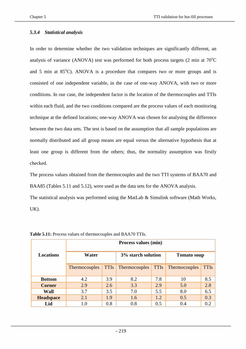
Chapter 5 TTI validation for hot-fill processes
- 219
5.3.4 Statistical analysis
In order to determine whether the two validation techniques are significantly different, an
analysis of variance (ANOVA) test was performed for both process targets (2 min at 70oC
and 5 min at 85oC). ANOVA is a procedure that compares two or more groups and is
consisted of one independent variable, in the case of one-way ANOVA, with two or more
conditions. In our case, the independent factor is the location of the thermocouples and TTIs
within each fluid, and the two conditions compared are the process values of each monitoring
technique at the defined locations; one-way ANOVA was chosen for analysing the difference
between the two data sets. The test is based on the assumption that all sample populations are
normally distributed and all group means are equal versus the alternative hypothesis that at
least one group is different from the others; thus, the normality assumption was firstly
checked.
The process values obtained from the thermocouples and the two TTI systems of BAA70 and
BAA85 (Tables 5.11 and 5.12), were used as the data sets for the ANOVA analysis.
The statistical analysis was performed using the MatLab & Simulink software (Math Works,
UK).
Table 5.11: Process values of thermocouples and BAA70 TTIs.
Locations
Process values (min)
Water 3% starch solution Tomato soup
Thermocouples TTIs Thermocouples TTIs Thermocouples TTIs
Bottom 4.2 3.9 8.2 7.8 10 8.5
Corner 2.9 2.6 3.3 2.9 5.0 2.8
Wall 3.7 3.5 7.0 5.5 8.0 6.5
Headspace 2.1 1.9 1.6 1.2 0.5 0.3
Lid 1.0 0.8 0.8 0.5 0.4 0.2

Chapter 5 TTI validation for hot-fill processes
- 220
1 1.5 2 2.5 3 3.5 40.05
0.10
0.25
0.50
0.75
0.90
0.95
Process values (min)
Pro
bab
ilit
yNormal Probability Plot
1 2 3 4 5 6 7 8
0.05
0.10
0.25
0.50
0.75
0.90
0.95
Process values (min)
Pro
bab
ilit
y
Normal Probability Plot
a. b.
0 1 2 3 4 5 6 7 8 9 100.05
0.10
0.25
0.50
0.75
0.90
0.95
Process values (min)
Prob
abili
ty
Normal Probability Plot
c.
Figure 5.14: Normal probability plots for a. Water, b. 3% starch solution and c. tomato soup. The left
and right hand lines refer to the BAA70 TTIs and thermocouples, respectively.
The scatter graphs give approximately straight lines through the first and third quartiles of the
data, indicating approximate normal distributions. In the case of 3% starch and tomato soup,
a slight departure from normality is observed in the lower tail. The shift in the mean from
thermocouples to TTIs is not strongly evident; Wilcoxon rank sum hypothesis test was used to
quantify that shift of distributions. The null hypothesis assumes that the two independent
samples come from continuous distributions with equal medians, whilst the alternative would
mean that they are not. If the null hypothesis is satisfied, the test will confirm that the shift
between the two samples is not significant.

Chapter 5 TTI validation for hot-fill processes
- 221
For all three fluids the logical output of h = 0, and the quite high p-values of approximately
0.6, indicate a failure to reject the null hypothesis at the default significance level of 1%.
Thus, the normality assumption was satisfied and the ANOVA test was next performed.
Table 5.12: ANOVA test for the correlation of BAA70 TTIs and thermocouples.
Source SS df MS F Prob>F
Water
Columns 0.144 1 0.144 0.09 0.7711
Error 12.72 8 1.59
Total 12.864 9
3% starch
Columns 0.9 1 0.9 0.09 0.7719
Error 80.076 8 10.0095
Total 80.976 9
Tomato soup
Columns 3.136 1 3.136 0.19 0.6728
Error 130.66 8 16.3325
Total 130.796 9
The ANOVA table shows the between-groups variation (Columns) and within-groups
variation (Error). SS is the sum of squares, and df is the degrees of freedom. MS is the mean
squared error, which is SS/df for each source of variation. The F-statistic is the ratio of the
mean squared errors, and the p-value is the probability that the test statistic can take a value
greater than or equal to the value of the test statistic.
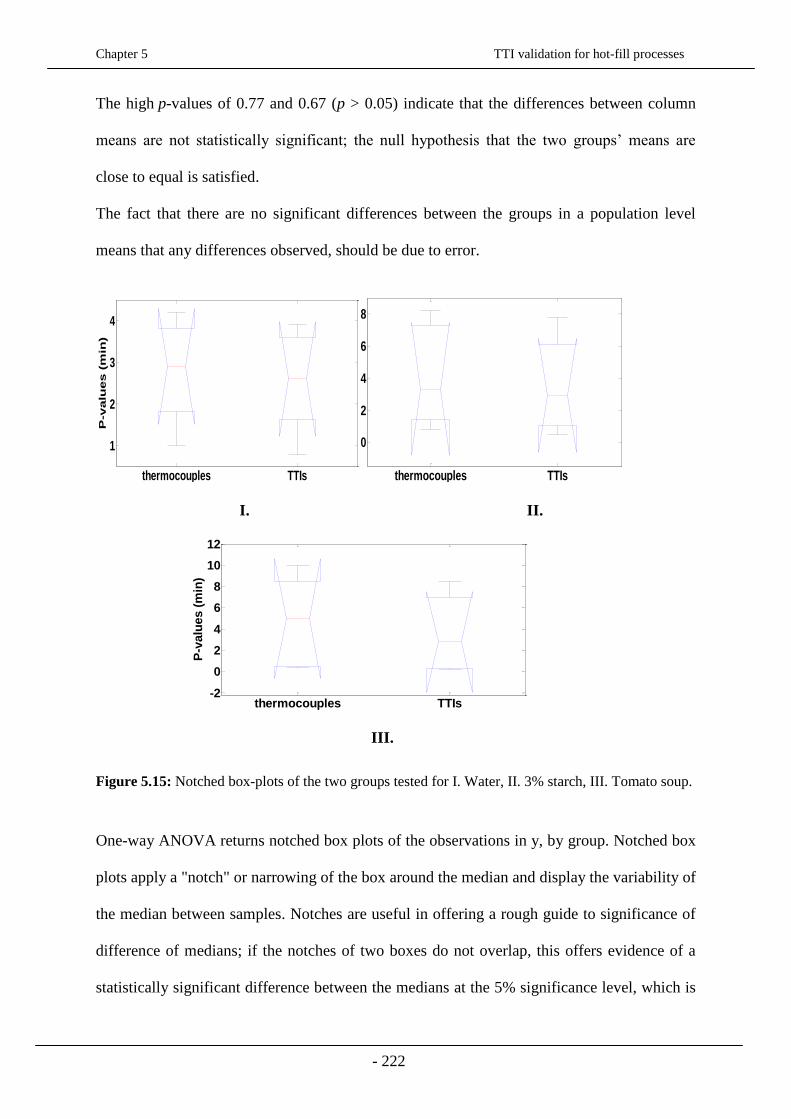
Chapter 5 TTI validation for hot-fill processes
- 222
The high p-values of 0.77 and 0.67 (p > 0.05) indicate that the differences between column
means are not statistically significant; the null hypothesis that the two groups’ means are
close to equal is satisfied.
The fact that there are no significant differences between the groups in a population level
means that any differences observed, should be due to error.
thermocouples TTIs
1
2
3
4
P-v
alu
es (
min
)
thermocouples TTIs
0
2
4
6
8
P-v
alu
es (
min
)
I. II.
thermocouples TTIs-2
0
2
4
6
8
10
12
P-v
alu
es (
min
)
III.
Figure 5.15: Notched box-plots of the two groups tested for I. Water, II. 3% starch, III. Tomato soup.
One-way ANOVA returns notched box plots of the observations in y, by group. Notched box
plots apply a "notch" or narrowing of the box around the median and display the variability of
the median between samples. Notches are useful in offering a rough guide to significance of
difference of medians; if the notches of two boxes do not overlap, this offers evidence of a
statistically significant difference between the medians at the 5% significance level, which is

Chapter 5 TTI validation for hot-fill processes
- 223
based on a normal distribution assumption. The width of the notches is proportional to the
interquartile range of the sample and inversely proportional to the square root of the size of
the sample. The "flipped" appearance in the notched box plots means that the 1st quartile has
a lower value than the confidence of the mean and vice versa for the 3rd quartile.
Figure 5.15 shows that the notches overlap, for all three fluids, indicating that there is no
significant statistical difference between the two mediums of each fluid at the 5%
significance level. This is confirmed by the low F-values and the high p-values, shown in the
ANOVA table. Thermocouples exhibit more heterogeneous values than TTIs, since the boxes
and the whiskers of thermocouples cover a larger range of the y-axis and its notches are
larger, which represents a larger dispersion of the data values for thermocouples (Gries
2009a: 204f).
The same procedure was followed for the second target, were thermocouples and BAA85
TTIs are the groups analysed. The normality of the data sets was firstly checked and was
followed by the Wilcoxon rank sum hypothesis test.
Table 5.13: Process values of thermocouples and BAA85 TTIs.
Locations
Process values (min)
Water 3% starch solution Tomato soup
Thermocouples TTIs Thermocouples TTIs Thermocouples TTIs
Bottom 2.0 1.8 3.0 2.5 2.7 2.5
Corner 1.6 1.5 1.8 1.7 1.8 1.6
Wall 1.9 1.7 2.4 1.8 2.5 2.2
Headspace 0.9 0.7 1.4 1.3 0.5 0.
Lid 0.6 0.4 1.3 1.0 0.3 0.1
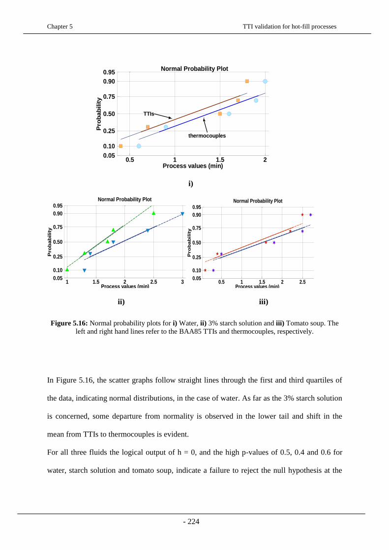
Chapter 5 TTI validation for hot-fill processes
- 224
0.5 1 1.5 20.05
0.10
0.25
0.50
0.75
0.90
0.95
Process values (min)
Pro
bab
ilit
y
Normal Probability Plot
thermocouples
TTIs
i)
1 1.5 2 2.5 30.05
0.10
0.25
0.50
0.75
0.90
0.95
Process values (min)
Pro
bab
ilit
y
Normal Probability Plot
0.5 1 1.5 2 2.50.05
0.10
0.25
0.50
0.75
0.90
0.95
Process values (min)
Pro
bab
ilit
y
Normal Probability Plot
ii) iii)
Figure 5.16: Normal probability plots for i) Water, ii) 3% starch solution and iii) Tomato soup. The
left and right hand lines refer to the BAA85 TTIs and thermocouples, respectively.
In Figure 5.16, the scatter graphs follow straight lines through the first and third quartiles of
the data, indicating normal distributions, in the case of water. As far as the 3% starch solution
is concerned, some departure from normality is observed in the lower tail and shift in the
mean from TTIs to thermocouples is evident.
For all three fluids the logical output of h = 0, and the high p-values of 0.5, 0.4 and 0.6 for
water, starch solution and tomato soup, indicate a failure to reject the null hypothesis at the

Chapter 5 TTI validation for hot-fill processes
- 225
default significance level of 1%. Thus, the normality assumption was satisfied and the
ANOVA test was next performed (Table 5.14).
Table 5.14: ANOVA test for the correlation of BAA85 TTIs and thermocouples.
Source SS df MS F Prob>F
Water
Columns 0.144 1 0.144 0.09 0.7711
Error 12.72 8 1.59
Total 12.864 9
3% starch
Columns 0.9 1 0.9 0.09 0.7719
Error 80.076 8 10.0095
Total 80.976 9
Tomato soup
Columns 3.136 1 3.136 0.19 0.6728
Error 130.66 8 16.3325
Total 130.796 9
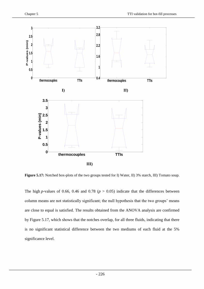
Chapter 5 TTI validation for hot-fill processes
- 226
thermocouples TTIs0
0.5
1
1.5
2
2.5
3P
-valu
es (
min
)
thermocouples TTIs0.4
1
1.6
2.2
2.8
3.2
P-v
alu
es (
min
)
I) II)
thermocouples TTIs0
0.5
1
1.5
2
2.5
3
3.5
P-v
alu
es (
min
)
III)
Figure 5.17: Notched box-plots of the two groups tested for I) Water, II) 3% starch, III) Tomato soup.
The high p-values of 0.66, 0.46 and 0.78 (p > 0.05) indicate that the differences between
column means are not statistically significant; the null hypothesis that the two groups’ means
are close to equal is satisfied. The results obtained from the ANOVA analysis are confirmed
by Figure 5.17, which shows that the notches overlap, for all three fluids, indicating that there
is no significant statistical difference between the two mediums of each fluid at the 5%
significance level.
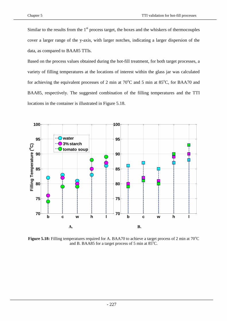
Chapter 5 TTI validation for hot-fill processes
- 227
Similar to the results from the 1st process target, the boxes and the whiskers of thermocouples
cover a larger range of the y-axis, with larger notches, indicating a larger dispersion of the
data, as compared to BAA85 TTIs.
Based on the process values obtained during the hot-fill treatment, for both target processes, a
variety of filling temperatures at the locations of interest within the glass jar was calculated
for achieving the equivalent processes of 2 min at 70oC and 5 min at 85
oC, for BAA70 and
BAA85, respectively. The suggested combination of the filling temperatures and the TTI
locations in the container is illustrated in Figure 5.18.
b c w h l70
75
80
85
90
95
100
Fil
lin
g T
em
pera
ture
(oC
)
b c w h l70
75
80
85
90
95
100
water
3% starch
tomato soup
A. B.
Figure 5.18: Filling temperatures required for A. BAA70 to achieve a target process of 2 min at 70oC
and B. BAA85 for a target process of 5 min at 85oC.

Chapter 5 TTI validation for hot-fill processes
- 228
5.4 Conclusions
Time Temperature Integrators (TTIs) were tested as an alternative validation method to
temperature sensors, for measuring pasteurisation treatments. The method uses an
encapsulated Bacillus amyloliquefaciens α-amylase (BAA) TTI, and it was applied to assess
hot-fill treatments targeting the two processes of 2 min at 70oC and 5 min at 85
oC for cook-
chilled and high acid food products, respectively. The TTIs were tested under isothermal and
tightly controlled non-isothermal conditions for the kinetic parameters to be obtained and for
testing their sensitivity to a variety of temperature profiles, respectively.
In the first set of experiments, the calibration of the two TTI systems resulted in a D70-value
of 4.1 min and a z-value of 10.8oC for BAA70 and a D85-value of 8.7 and a z-value of 10.3
oC
for BAA85. The z-values of both enzymes are consistent with the values required for
pasteurization processes, but higher than the values of the target processes, (7.5oC, and 8.3
oC,
respectively), which lead to underestimation of the thermal process. For overcoming this
problem, the TTIs were submitted to temperatures higher than the reference ones, at 75 and
90oC, for predicting real process time and for being consistent with the heat duration time
estimated from the isothermal experiments; the maximum heat duration was calculated to be
7 and 16 min for BAA70 and BAA85, respectively.
In the second set of experiments, TTIs were tested under non-isothermal conditions using the
Peltier stage, which generated various time-temperature profiles under constant
heating/cooling rate for a variety of holding times (simple cycles) and subsequent
heating/cooling with no holding time (complex cycles). The TTIs appeared to pick up small
temperature differences, but they do not reach the temperature that the Peltier stage is set to
deliver; both BAA70 and BAA85 TTIs recorded temperatures 5 to 8oC lower than the
thermocouples. That is possibly due to the silicone tube thickness, which acts like a barrier in
transferring the applied heat, the higher conduction received by the thermocouples and the
Chapter 5 TTI validation for hot-fill processes
- 229
limitations coming from the assay method and the spectrophotometer. Another possible
problem with the design of the specific TTIs is that the majority of their volume is positioned
above the surface of the package, which means that only a small area of the TTIs will be in
contact with the surface. Thus, in the case that there is a large temperature difference between
the surface of the package and the bulk of the fluid, the TTIs would be exposed to a
temperature slightly higher than that of the package, resulting to higher process values.
After the sensitivity tests were performed, the response of the TTIs was investigated under
the hot-fill treatment conditions, and was compared to that of the temperature sensors under
the same conditions and locations. The two monitoring techniques were compared for a
filling temperature of 75 and 90oC, for BAA70 and BAA85, respectively, with water, 3% of
starch solution and tomato soup being the heating mediums. The process values were
calculated at five different positions inside the glass jar, as shown in Figure 2.11, with the
headspace and the lid being the coldest points. The target process was achieved by the
bottom, bottom-corner and wall for BAA70 TTI and all three fluids. The filling temperature
was not sufficient to pasteurise the headspace and the lid. The time-temperature combination
of 10 min at 90oC, did not achieve the target process of 5 min at 85
oC, with the TTIs showing
lower process values than the thermocouples. Both TTI systems record lower temperatures
than thermocouples under any of the conditions they were submitted in the current work. In
order to investigate whether the two validation methods are significantly different, a
statistical analysis of variance was performed. Results from the ANOVA tables and the box-
plots, showed that the two methods are statistically not significantly different at a 5%
confidence level. That means that the agreement between the two methods can be considered
to be good, given the potential for discrepancy; the TTI systems could be safely used for
evaluating pasteurisation processes.

Chapter 5 TTI validation for hot-fill processes
- 230
References
Banga J.R., Perez-Martín R.I., Gallardo J.M., Casares J.J., (1991). Optimisation of thermal
processing of conduction-heated canned foods: study of several objective functions. Journal
of Food Engineering, 14, 25.
Bellara S.R., Fryer P.J., McFarlane C.M., Thomas C.R., Hocking P.M., Mackey B.M.,
(1999). Vizualization and modelling of the thermal inactivation of bacteria in a model food.
Applied Environmental Microbiology, 65, 3095-3099.
Brown K.L., Ayres C. A., Gaze J. E., and Newman, (1984). Thermal destruction of bacterial
spores immobilised in food/alginate particles. Food Microbiology, 1:187-198.
Bobelyn Els, Hertog Maarten, Nicolaï Bart M., (2006). Applicability of an enzymatic time
temperature integrator as a quality indicator for mushrooms in the distribution chain.
Postharvest Biology and Technology, 42(1):104–114.
Campden & Chorleywood Food Research Association (CCFRA), (1992a). Food
Pasteurisation Treatments. Technical Manual No.27.
Campden & Chorleywood Food Research Association (CCFRA), (2006b). Pasteurisation: A
food industry practical guide (second edition). Guideline No.51.
De Cordt S., Hendrickx M., Maesmans G., and Tobback P. (1992). Immobilised -amylase
from Bacillus licheniformis: a potential enzymic time-temperature integrator for thermal
processing. International Journal of Food Science and Technology, 27, 661-673.
De Cordt S., Avila I., Hendrickx M. & Tobback P., (1994). DSC and protein-based time
temperature integrators: Case study of -amylase stabilised by polyols and/or sugar.
Biotechnology & Bioengineering, 44, 859-865.
Fryer P. J., Simmons M.J.H., Cox P.W., Mehauden K., Hansriwijit Suwijak, Challou Flora,
Bakalis Serafim, (2011). Temperature Integrators as tools to validate thermal processes in
food manufacturing. Procedia Food Science, 1:1272–1277, 11th International Congress on
Engineering and Food (ICEF11).
Gries S. T., (2009a). Quantitative corpus linguistics with R. A practical introduction. London:
Routledge.
Guiavarc‟h Y., (2003). Development and use of enzymic time-temperature integrators for the
assessment of thermal processes in terms of food safety. PhD Thesis No.570, Katholike
Universiteit Leuven, Belgium.
Chapter 5 TTI validation for hot-fill processes
- 231
Hendrickx M., Saraiva J., Lyssens J., Oliveira J. & Tobback P., (1992). The influence of
water activity on thermal stability of horseradish peroxidase. International Journal of Food
Science & Technology, 27, 33-40.
Hendrickx M., De Cordt S., Van Loey., (1995). Evaluation of the integrated time‐temperature
effect in thermal processing of foods. Critical Reviews in Food Science and Nutrition, 35(3).
Jin Q., Jin W., Guanglin Z., Qin F., (2012). A time–temperature indicator based on
glucoamylase. China Patent 201110394281.X.
Kim W., Park E., Hong K., (2012). Development of a time–temperature integrator system
using Burkholderia cepacia lipase. Food Science and Biotechnology, 21:497–502.
Maesmans G., Hendrickx M., De Cordt S., Van Loey A., Noronha J., Tobback P., (1994).
Evaluation of process value distribution with time temperature integrators. Food Research
International, 27, 413-423.
Moles C.G., Alonso A. A., (2003). Improving food processing using modern optimization
methods. Trends in Food Science & Technology 14 (4), 131-144.
Moritz M., Balasa A., Jaeger H., Meneses N., Knorr D., (2012). Investigating the potential of
polyphenol oxidase as a temperature–time-indicator for pulsed electric field treatment. Food
Control, 26:1–5.
Mulley E.A., Stumbo C.R. and Hunting W.M., (1975). Thiamine: A chemical index of the
sterilization efficacy of thermal processing. Journal of Food Science, 40: 993.
Tucker G.A., and Holdsworth S.D., (1996). Optimization of Quality factors for Foods
Thermally Processed in Rectangular Containers. Technical Memorandum 627, CCFRA,
Chipping Campden, UK.
Tucker G.S., (1999). A novel validation method: Application of time-temperature integrators
to food pasteurization treatments. Transactions of the IChemE, Food and Bioproducts
Processing, 77, Part C, 223-231. Campden and Chorleywood Food Research Association,
Chipping Campden, UK.
Tucker G.S., Lambourne T., Adams J.B., and Lach A., (2002). Application of biochemical
time-temperature integrators to estimate pasteurisation values in continuous food processes.
Innovative Food Science & Emerging Technologies, 8 (1), 63-72.
Tucker G.S. and Wolf D., (2003). Time-temperature integrators for food process analysis,
modelling and control. R&D Report No.177. Campden & Chorleywood Food Research
Association.
Tucker S., Brown H.M., Fryer P.J., Cox P.W, Poole F.L., Lee H.S., (2007). Sterilisation
time–temperature integrator based on amylase from the hyperthermophilic
organism Pyrococcus furiosus. Innovative Food Science & Emerging Technologies, 8:63–72.
Chapter 5 TTI validation for hot-fill processes
- 232
Van Loey A., Hendrickx M., De Cordt M.E., Haentjens T.H and Tobback P.P., (1996).
Quantitative evaluation of thermal processes using time-temperature integrators. Trends in
Food Science and Technology, 7, 16-26.
Van Loey A., Arthawan A., Hendrickx M., Haentjens T.H. and Tobback P.P., (1997a). The
development and use of an a-amylase based time-temperature integrator to evaluate in-pack
pasteurization processes, Lebensmittel-Wissenschaft und-Technologie, 30: 94 –100.
Van Loey A., Guiavarc'h Y., Claeys W., Hendrickx M., (2004). Improving the thermal
processing of foods: The use of time–temperature integrators (TTIs) to validate thermal
processes. P. Richardson (Ed.), Woodhead Publishing Ltd., Cambridge, UK p. 365–379.
Yan S., Huawei C., Limin Z., Fazheng R., Luda Z., Hengtao Z., (2008). Development and
characterization of a new amylase type time–temperature indicator. Food Control, 19:315–
319.

Chapter 6 Conclusions and Future Work
- 233
Chapter 6 - Conclusions and Future Work
6.1 Conclusions
In this thesis, the inversion method was investigated for its effectiveness as a thermal
treatment of the headspace and the lid, for hot-filled model foods. Starch solutions and cream
of tomato soup were used for evaluating a heat treatment targeting a process of 5 min at 70oC.
The model fluids were hot-filled in pre-heated glass jars at a temperature of 80oC, were
inverted for 30 s, brought back to the upright position and cooled at room temperature for 10
min. The chosen set of inversion time and filing temperature appeared to be sufficient for
achieving the goal set, for the least viscous fluids, 3% and 4% starch solution, whilst it was
not for the tomato soup and the 5% starch solution (the most viscous fluid). The inverted jars
showed significantly higher process values for the headspace and the lid with the filling
temperature being the most important parameter.
The behaviour of the model fluids was investigated by carrying out a series of rheological
experiments and developing a dynamic mathematical model. Results showed a shear-thinning
behaviour for all model fluids, with dominating elastic properties, and the finite element
method used, based on dimensionless numbers and the viscosities calculated from the steady
state rheological test, indicated that the fluids could generate natural convection from the
lateral boundaries. The temperature distribution and flow behaviour of tomato soup and 3%
starch solution for the inverted and non-inverted packages, was further analysed and
predicted mathematically using the finite element method; the predicted data were compared
with the experimental ones, for validating the model. A two-dimensional, axi-symmetrical

Chapter 6 Conclusions and Future Work
- 234
geometry was used for computational simplification and fluids were assumed to have
constant thermo-physical properties, but temperature dependant viscosity. 7031 nodal points
were used with a finer grid near the walls and the interface of air-fluid with a convergence
criterion set to 10-8
. For both fluids and cases investigated, the temperature isotherms and
velocity vectors plotted, showed that cold zones are located near the walls and the interface
between the fluid and air. The convection currents push the cold zones of the fluid to move
from the headspace towards the bottom of the jar and near the wall, creating secondary and
tertiary flows. The forced convection caused by the inversion of the package, created higher
recirculation within the fluid; the disrupted interface of the fluids indicated the existence of
either a bubble created during inversion or the movement of cold spots within the fluid. The
velocity values of fluid A (7.8 x 10⁻³
) were up to ten times higher than those in fluid T(6.3 x
10-4
), explaining the faster heating of the headspace and the lid and the lower temperatures
observed. The comparison of the predicted temperature profiles with the experimental ones
showed good agreement for both cases and fluids. The correlation of the two data sets was
confirmed by the low RMSE values obtained, validating the model developed.
The heat treatment of hot-filling was also evaluated by Bacillus amyloliquefaciens α-amylase
(BAA) based Time Temperature Integrators (TTIs), which are used as an alternative
validation method to temperature sensors. The method was applied to target the two
processes of 2 min at 700C and 5 min at 85
0C for cook-chilled and high acid food products,
respectively. The TTIs were tested under isothermal conditions, resulting in a D70-value of
4.1 min and a z-value of 10.80C for BAA70 and a D85-value of 8.7 and a z-value of 10.3
0C
for BAA85; the heat duration of BAA70 and BAA85 was 7 and 16 min, respectively. The
TTIs appeared to pick up small temperature differences, when tested under tightly controlled,
non-isothermal conditions but, they consistently record temperatures lower than the
thermocouples. The ANOVA statistical analysis conducted showed that the two monitoring

Chapter 6 Conclusions and Future work
techniques are statistically not significantly different at a 5% confidence level, indicating that
the correlation between the thermocouples and the TTIs can be considered to be good, given
the potential for discrepancy. Thus, the TTI systems could be safely used for evaluating
pasteurisation processes.
6.2 Future work
The inversion of glass packages as a thermal treatment of the headspace and the lid has been
shown to be promising for targeting yeasts and moulds in acid foods. Further studies on a
variety of inversion time and filling temperature combinations could help reduce the time of
post-pasteurisation treatments used currently in the food industry. Different package
materials and sizes could also be investigated in evaluating the effectiveness of the inversion
step. Preliminary experiments on hot-fill treatments with Polyethylene terephthalate (PET)
and carton packages showed a noticeable difference in the effectiveness of the method,
expressed in terms of process values. That is due to the significantly different thermal
properties of the package material making them worth investigating. The two materials and
the different package sizes were not expanded in this work due to time limitation.
The use of temperature sensors for validating the degree of thermal process achieved will
probably remain the most used method, since on-line process control is feasible, as compared
to the TTIs. Both the temperature sensors and the TTIs lack predictive power for processing
conditions different from the ones under which the experiments are run. Thus, advanced
mathematical models have been developed in the last decades to overcome that problem and
predict process times and temperatures based on empirical formulae or theoretical heat
transfer models. Most of the food companies rely on the General method for setting up time-
temperature plans, but the method does not allow process deviations to be assessed. By the
Chapter 6 Conclusions and Future Work
- 236
use of predictive modeling the batches of food products that undergo process deviation,
would be able to be controlled and the process establishment would be more straightforward
(Tucker et al., 2003). Based on experiments from current work, modelling the heat process
would potentially show by how much the temperature difference between the two monitoring
techniques can underestimate the process and what would the ideal filling temperature be for
the best correlation.
TTIs would be very advantageous if combined with temperature sensors; being used in
monitoring critical control points is fundamental. In traditional canning process, lethal rates
are evaluated at time steps of one minute, due to current capabilities of data loggers, but with
modern processes they can be estimated at time steps of one second. The application of TTIs
to various thermal processes, such as pasteurisation and sterilisation is active, especially for
food products that are heated and cooled in large vessels or heat exchangers where wire-
based systems cannot be used.