surface exposure cosmogenic nuclide dating - · pdf fileexposure dating that cosmogenic...

Cosmogenic nuclide dating 1

Title: Surface exposure cosmogenic nuclide dating

Author: Kerry J. Cupit

Location:

Simon Fraser University

8888 University Drive

Burnaby, B.C.

Canada V5A 1S6

Contact email: [email protected]

Contact address:

10543 170A Street

Surrey, B.C.

Canada V4N 5H8

Running title: Cosmogenic nuclide dating

Keywords: cosmogenic, geochronology, dating techniques, radioisotopes, isotopes, cosmic rays

Date submitted: April 1, 2008


Abstract

Title: Surface exposure cosmogenic nuclide dating

Author: Kerry J. Cupit, Department of Earth Sciences, Simon Fraser University

Using radiometric dating techniques to solve problems in quaternary geology was not

possible until twenty years ago with the advent of commonplace accelerator mass spectrometers.

Building upon theories developed in the 1950s, enough research has been made into surface

exposure dating that cosmogenic nuclide dating has proven itself as an effective tool for

measuring absolute ages that every quaternary geologist should keep in their analytical arsenal.

Emanating from the centre of the Milky Way galaxy is a steady stream of randomly

oriented cosmic rays, ionized particles traveling at relativistic speeds. These rays interact with

the Earth’s geomagnetic field, atmosphere and lithosphere, whereby they attenuate according to

the density of the matter they are passing through. By measuring the daughter products produced

by collisions of cosmic rays with terrestrial matter (cosmogenic nuclides), it is possible to obtain

absolute ages of surface exposures. Cosmogenic nuclide dating has found applications in

measuring erosion rates and dating landforms like landslides, recent lava flows, moraines, fluvial

and alluvial landforms and faults. It is also finding use in the field of archaeology. Cosmogenic

nuclide dating requires careful correction for variability in space and time of the geomagnetic

field, solar plasma flux, galactic cosmic ray flux, atmospheric density.


(A) Introduction

(B) Theory (i) Origin of cosmic rays (ii) Cosmic ray interactions (iii) Nuclide production rates (iv) Attenuations (v) Complexities (C) Nuclides (i) Helium-3 (ii) Neon-21 (iii) Argon-38 (iv) Beryllium-10 (v) Aluminium-26 (vi) Chlorine-36 (vii) Carbon-14 (D) Applications (i) Erosion rates (ii) Landslides (iii) Lava flows (iv) Glaciers (v) Fluvial and alluvial landforms (vi) Faults (vii) Archaeology (E) Conclusion

(F) References

(G) Tables

(H) Figures


(A) Introduction

Many dating techniques are available to quaternary geoscientists, but each have inherent

and varied complications that can limit their utility. As technology develops, so too will

analytical techniques allowing for more precise dates to be obtained over a broader range of

time. The process of cosmogenic nuclide dating embodies this well, with advances in

technology in the last twenty years opening up a new realm of quaternary dating for exposed

surfaces as young as ten years and as old as thirty million years (Schaefer and Lifton 2007).

Introduced as a way to date geological and archeological Quaternary materials,

cosmogenic nuclide dating incorporates a lot of past work in experimental physics, analytical

chemistry, geochemistry, geomorphology and geophysics (Gosse 2007). Theorized by Libby in

the 1950s (Gosse 2007), it has found use in dating landforms like terminal moraines, fluvial

incisions, alluvial terraces and fans, landslide deposits and lava flows (Desilets 2005). However,

surface exposure cosmogenic nuclide dating isn't without its problems. If necessary corrections

aren't meticulously accounted for, dates resulting from this technique may be imprecise

(Schaefer and Lifton 2007). This paper explores the theory behind cosmogenic nuclide

production, their accumulation rates in surficial geologic materials, known and future

applications for this technique, and the numerous complexities involved in ensuring dates

returned are reliable.

(B) Theory

The theory governing the applicability of measuring cosmogenic nuclides to quaternary

dating is rooted in research undertaken by researchers like Lal and Peters (1967), Raymond

Davis and Oliver Schaffer (Gosse and Phillips 2001). However, it was impossible at the time


these theories were proposed to measure nuclide concentration ratios down to the 10-15 required

for this technique (Gosse and Phillips 2001), due to a lack of suitably sensitive equipment. With

the further development of accelerator mass spectrometry in the 1980s, cosmogenic nuclide

dating began to flourish. Previously, techniques such as thermoluminescence were used in lieu

of additional options now presented through the modern analysis of cosmogenic nuclides (Lal

2007).

(i) Origin of cosmic rays

Throughout the universe, four primary types of radiations can be found: electromagnetic

radiation, cosmic radiation, neutrinos and gravitational radiation (Lal 2007). Of these, cosmic

radiation plays an important role in the production of cosmogenic nuclides in surficial materials

on Earth, and forms the basis of cosmogenic nuclide dating. Essentially, cosmic radiation (often

referred to as "cosmic rays") consists of normal matter that has been accelerated to near-light

speed by the shock waves produced from supernovae within the Milky Way galaxy (Lal 2007;

Gosse and Phillips 2001). This matter is ionized, having been stripped of electrons (Lal 2007).

Since hydrogen is the most abundant element in the universe, it is reasonable to expect that many

cosmic rays follow this proportion, with lesser amounts of helium, carbon, nitrogen and oxygen

making up the residual, and indeed this is what many cosmic ray experiments have found (Lal

2007). Flares on the surfaces of other Milky Way stars are also a source of cosmic rays, but

aren't as significant a contributor as supernovae. With approximately three supernovae in the

galaxy occurring per century (Lal 2007), there is a constant source of this material interacting

with the Earth throughout geologic time.


(ii) Cosmic ray interactions

The interaction of cosmic rays with normal matter is a function of the density of the

material they happen to be passing through (Gosse 2007). As cosmic rays approach the Earth at

relativistic speeds (Lal 2007) from the near vacuum of space into the denser levels of Earth's

atmosphere, the chance that the ray will impact another atom is increased with atmospheric

depth. In fact, when the phase of matter is solid as is the case with the Earth's crust, the furthest

penetration of cosmic rays can be measured over a few centimetres to a few metres before they

are stopped completely (Gosse 2007; Schaefer and Lifton 2007).

When a cosmic ray interacts with a terrestrial atom, many subatomic and atomic particles

are ejected from the impact site through a process known as spallation (Gosse 2007; Schaefer

and Lifton 2007; American Geological Institute 2008; Lal 2007). While the initial reaction

between a cosmic ray and an atom is referred to as primary radiation, the particles produced in

this first stage can lead to secondary radiation, whereby a shower of secondary particles can react

with other nearby terrestrial nuclei (Gosse 2007; Schaefer and Lifton 2007; Lal 2007). Both

forms result in the formation of nuclides that are identifiable as having a cosmogenic origin,

mainly through their isotopic rarity relative to average isotopic ratios in the Earth's crust.

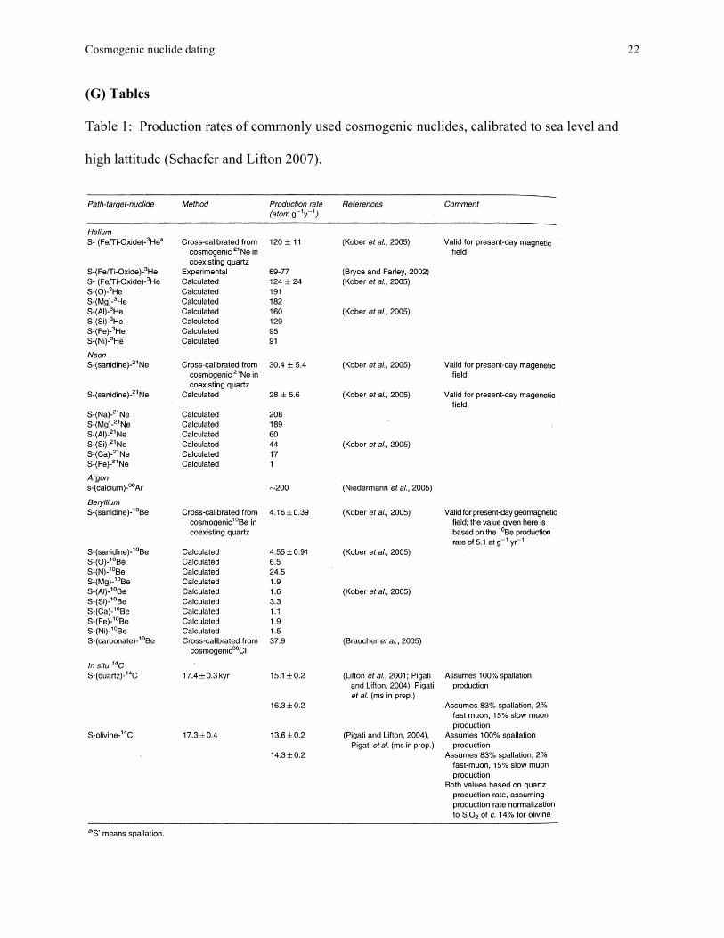
(iii) Nuclide production rates

In order to use the concentrations of cosmogenic nuclides within a rock to date an

exposure, typical rates of nuclide production need to be known to relate them to a chronological

date (Schaefer and Lifton 2007). Production rates can be estimated in one of three different

ways. First, by independently dating a surface exposure through other techniques such as

thermoluminescence or radiocarbon dating, it is possible to calibrate the results produced by two


distinct procedures and therefore infer a nuclide production rate (Schaefer and Lifton 2007).

However, the effect of erosion removing the top layers of a surface exposure over time can result

in underestimates of production rates, since the topmost layers, those containing the greatest

abundance of cosmogenic nuclides, are no longer present (Ivy-Ochs and Kober 2007). To that

end, cosmogenic nuclide production rates can also be estimated by locating an almost erosion-

free surface and analyzing the cosmogenic nuclides retained (Schaefer and Lifton 2007). Due to

the radioactive decay of cosmogenic nuclides, a surface exposure will reach saturation

equilibrium after about 5 half-lives of the nuclide being analyzed (Schaefer and Lifton 2007).

Therefore, if erosion can be assumed to be negligible, then a production rate of a particular

cosmogenic nuclide can be estimated by relating a total concentration at a surface exposure to

the amount of time passed equal to five half-lives.

The third and most complicated estimation of cosmogenic nuclide production rates is

through the careful theoretical modeling of cosmic ray pathways and interactions (Schaefer and

Lifton 2007). However, the majority of nuclide production rate studies use independently dated

surfaces to relate their results (Schaefer and Lifton 2007). Many of these estimations on

cosmogenic nuclide production rates are summarized in Table 1.

(iv) Attenuations

Cosmic rays will attenuate as they interact with matter (Lal 2007), resulting in fewer

remaining rays present at greater depths within the atmosphere and lithosphere (Gosse 2007; Ivy-

Ochs and Kober 2007; Granger 2007). In the atmosphere, the total number of cosmic ray

interactions has been estimated from observations of nuclear emulsions and cloud chambers at

different altitudes and latitudes (Lal 2007). From these experiments, researchers have concluded


that cosmogenic nuclide production rates at sea level and at the top of the atmosphere can vary

by a factor of 0.0015 - 0.0100 (Lal 2007).

Less than 1% of the atmosphere lies above a height of 32 km above the Earth's surface

(Gosse and Phillips 2001). However, the strength of the geomagnetic field at a height of 1600

km is only half of what it is at the Earth's surface (Gosse and Phillips 2001). Given that cosmic

rays are ionized (Lal 2007) and thus have a charge, most incoming cosmic rays will therefore

experience deflection forces long before they interact significantly with the atmosphere. The

geomagnetic field measurably attenuates cosmic rays (Lal 2007), however Desilets (2005) found

that the magnitude of this effect is dependent upon the geomagnetic coordinates at a particular

site and the field strength associated with such, due to the asymmetry of the global geomagnetic

field.

Primary and secondary cosmic radiation reaching the surface of the Earth will attenuate

very quickly relative to lithospheric depth, with most rays attenuated within the first metre

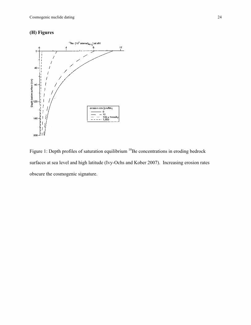
(Granger 2007). Depending on the cosmogenic nuclide being analyzed, some nuclides like 10Be

are regularly detected at depths greater than 5 metres (Gosse 2007). Figure 1 shows a depth

profile of 10Be formation at an exposed surface. Gosse (2007) found that attenuation depends

upon the bulk density of the rock, sediment or soil that is exposed. It would stand to reason that

this same principle can be applied to atmospheric attenuation, or attenuation attributable to

snow/ice cover, where different densities can result in cosmogenic nuclides found at deeper or

shallower depths in a particular medium.

Additionally, solar plasma can interfere with cosmic rays (Desilets 2005; Schaefer and

Lifton 2007; Lal 2007) even before an incoming ray interacts significantly with Earth's

geomagnetic or atmospheric systems. There is also the added effect of radioactive decay of


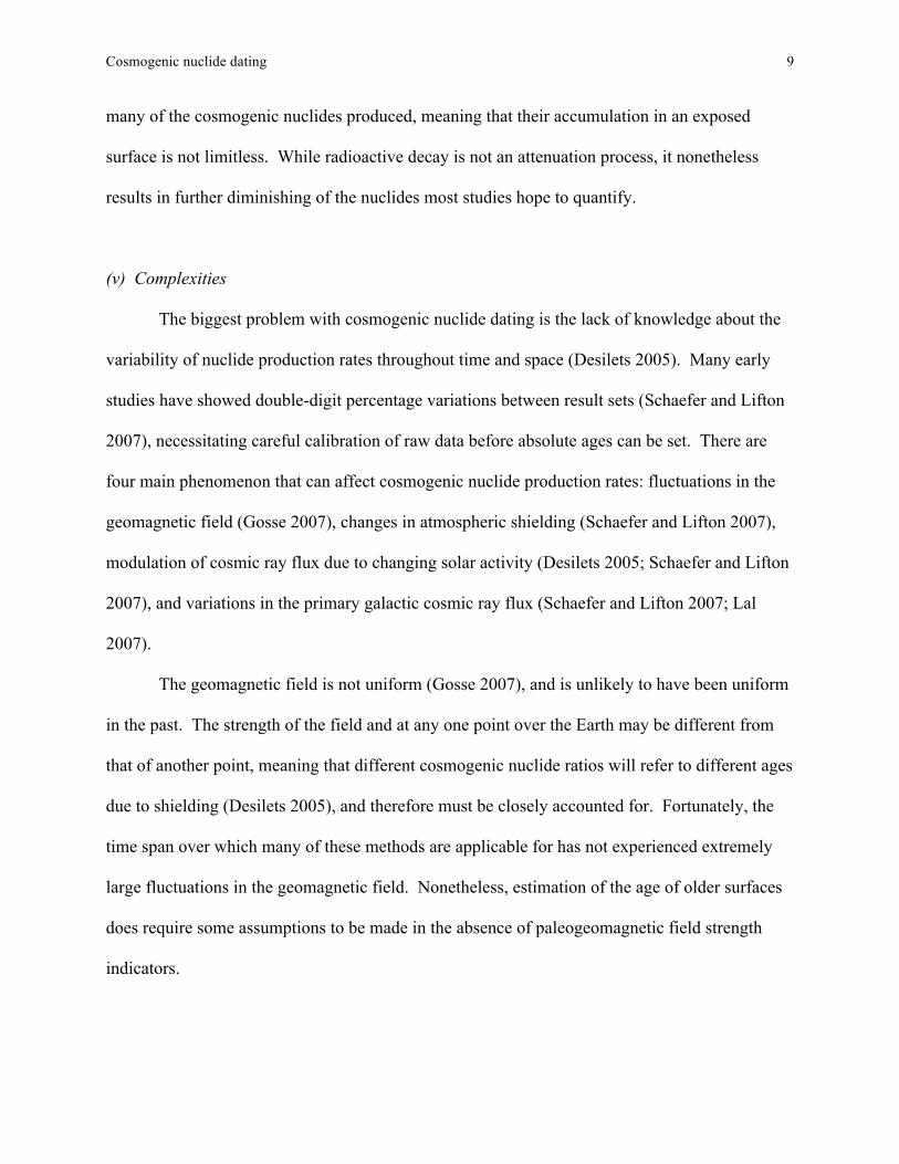
many of the cosmogenic nuclides produced, meaning that their accumulation in an exposed

surface is not limitless. While radioactive decay is not an attenuation process, it nonetheless

results in further diminishing of the nuclides most studies hope to quantify.

(v) Complexities

The biggest problem with cosmogenic nuclide dating is the lack of knowledge about the

variability of nuclide production rates throughout time and space (Desilets 2005). Many early

studies have showed double-digit percentage variations between result sets (Schaefer and Lifton

2007), necessitating careful calibration of raw data before absolute ages can be set. There are

four main phenomenon that can affect cosmogenic nuclide production rates: fluctuations in the

geomagnetic field (Gosse 2007), changes in atmospheric shielding (Schaefer and Lifton 2007),

modulation of cosmic ray flux due to changing solar activity (Desilets 2005; Schaefer and Lifton

2007), and variations in the primary galactic cosmic ray flux (Schaefer and Lifton 2007; Lal

2007).

The geomagnetic field is not uniform (Gosse 2007), and is unlikely to have been uniform

in the past. The strength of the field and at any one point over the Earth may be different from

that of another point, meaning that different cosmogenic nuclide ratios will refer to different ages

due to shielding (Desilets 2005), and therefore must be closely accounted for. Fortunately, the

time span over which many of these methods are applicable for has not experienced extremely

large fluctuations in the geomagnetic field. Nonetheless, estimation of the age of older surfaces

does require some assumptions to be made in the absence of paleogeomagnetic field strength

indicators.


Air pressure variations can result in density differences that reduce or increase the

amount of attenuation of cosmic rays by the atmosphere (Schaefer and Lifton 2007). In

Antarctica for example, Schaefer and Lifton (2007) found evidence for a 30% increase in nuclide

production rates due to a 25 hPa lower air pressure difference between Antarctica and other

continents. Furthermore, other researchers have suggested that during periods of extensive

glaciation, atmospheric pressures are depressed as evidenced from atypical 39Ar/40Ar ratios in

lavas formed 70 thousand to 110 thousand years ago (Stone 2000). Assumptions are regularly

made about fluctuations in atmospheric pressure, and Stone (2000) has published global

correction factors suggested for use in all cosmogenic nuclide studies.

Solar wind particles can attenuate cosmic rays, and the output of solar wind into the solar

system is governed by the Sun's 11-year solar cycle. These cycles must be accounted for, in

regards to calculating typical nuclide production rates at a specific point in time (Schaefer and

Lifton 2007).

Cosmic ray intensity will vary over time (Schaefer and Lifton 2007; Lal 2007). Short

term dating techniques spanning 101 - 106 years need not consider this (Schaefer and Lifton

2007). However, over longer time periods data may need to be corrected for this effect. If a

supernova occurs nearby our solar system, significant increases in cosmic ray intensity will result

(Lal 2007), possibly greatly affecting the cosmogenic nuclide signature in surface exposures

from that time.

(C) Nuclides

A number of nuclides are produced from cosmic radiation (Gosse 2007; Schaefer and

Lifton 2007; Lal 2007), each with a different half-life and each requiring different analytical


techniques to identify them (Gosse 2007; Schaefer and Lifton 2007; Ivy-Ochs and Kober 2007).

The ideal technique to use in any one situation will depend on which minerals and lithologies are

involved (Gosse 2007). Additional factors to consider are the analytical limits of the mass

spectrometer, sufficient exposure time at a site, nuclide production rate and depth at a site, the

number of samples needed, the abundance of non-cosmogenic species of the same isotope,

diffusion constraints, and the complexity of a sample's exposure, burial and re-exposure history

(Gosse 2007). All techniques require high precision atomic-grade noble gas spectrometers or

accelerator mass spectrometers (Gosse 2007). Typical nuclides used in cosmogenic nuclide

dating include 3He, 21Ne, 38Ar, 10Be, 26Al, 36Cl and 14C.

(i) Helium-3

Helium-3 has a well-calibrated production rate and a wide applicable dating range from

103 - 107 years (Schaefer and Lifton 2007). It is retained in minerals such as pyroxenes, olivine

and garnet (Gosse 2007; Schaefer and Lifton 2007), although getting pure mineral samples for

analysis can be difficult. Some researchers have applied 3He dating to quartz, however most

have found that 3He diffuses too quickly from quartz to make it useful (Gosse 2007; Schaefer

and Lifton 2007). One particular challenge is separating out cosmogenic helium from mantle

helium (Schaefer and Lifton 2007).

(ii) Neon-21

Neon-21 is analyzed from quartz, olivine, pyroxene and recently sanidine (Schaefer and

Lifton 2007). It is less well calibrated than other noble gases used in nuclide studies, like

helium-3, however it has the largest useful range of all the nuclides. It is useful for obtaining


absolute ages in the range of 104 years to 3 x 107 years (Schaefer and Lifton 2007). However,

neon-21 dating isn't as commonplace due to the difficulties in preparing samples for analysis

(Schaefer and Lifton 2007). Analysis of other nuclides may be more cost effective.

(iii) Argon-38

The youngest and most experimental of all the cosmogenic dating techniques is argon-38

(Gosse 2007). It is produced mainly from spallation of potassium and calcium atoms (Schaefer

and Lifton 2007), and therefore can be found in minerals rich in those elements. However, due

to the difficulty of determining the origin of some argon isotopes, namely those produced by

neutron capture by chlorine-36, it is recommended that minerals to be analyzed be devoid of

chlorine and potassium altogether (Schaefer and Lifton 2007).

(iv) Beryllium-10

Beryllium-10 is the workhorse of modern cosmogenic nuclide dating, due to its well-

constrained production rate and its large applicable age range (Schaefer and Lifton 2007). It is

not uncommon to use beryllium-10 to date materials spanning 101 to 106 years, with some

applications extending ages up to 3 to 4 million years (Schaefer and Lifton 2007). Cosmogenic

beryllium-10 can be found in quartz, calcite and sanidine (Schaefer and Lifton 2007), yet it has a

six-fold higher production rate in calcite than in quartz (Braucher et al. 2005).

(v) Aluminium-26

With a half-life of 0.7 million years (Gosse 2007), aluminum-26 is used for dating

exposures with absolute ages between 103 and 106 years old (Schaefer and Lifton 2007). Its


analytical uncertainty is poorer than that of beryllium-10, but it is easily extracted from the same

quartz samples used in beryllium-10 analyses (Schaefer and Lifton 2007), resulting in both 26Al

and 10Be often being employed in studies. Its cosmogenic production rate is nearly as well

known as that for beryllium-10 (Schaefer and Lifton 2007).

(vi) Chlorine-36

While other cosmogenic nuclides require careful selection and analysis of individual

mineral grains, chlorine-36 can be calibrated using whole rock samples (Gosse 2007), therefore

any lithology can be used for cosmogenic 36Cl analysis. Apart from obvious cost savings in

sample preparation, a significant benefit of this technique is that aphyric lavas can also be dated

(Ivy-Ochs and Kober 2007), which is extremely difficult or altogether impossible to do using

other cosmogenic nuclides. Despite this convenience, the most representative way to determine

ages from chlorine-36 is to use mineral separates whenever possible (Schaefer and Lifton 2007).

(vii) Carbon-14

Carbon-14 has a half-life of 5.7 thousand years (Gosse 2007), the shortest of all the

cosmogenic nuclides. It is therefore useful in calculating absolute ages for more recent

landforms than other isotopes with a longer half-life, with the possible of exception of beryllium-

10. While carbon-14 can be relatively difficult to prepare, involving acid etching and stepwise

combustion (Schaefer and Lifton 2007), it is easy to calibrate. After five half lives, the

production and decay of cosmogenic carbon-14 on an exposure is in equilibrium, allow for easy

measurement of a maximum baseline concentration (Schaefer and Lifton 2007; Ivy-Ochs and

Kober 2007). This is the same technique used to constrain nuclide production rates of other


cosmogenic nuclides, however the shorter half-life of carbon-14 means that surfaces need only

be exposed for a minimum of 25 thousand years, making it useful for erosion studies and

preliminary cosmogenic nuclide dating studies.

Carbon-14 has usually been employed in rocks of felsic or intermediate composition.

However, some researchers have found success in employing it to analyze mafic minerals,

particularly olivine (Schaefer and Lifton 2007). Dates obtained are sensitive to the ratio of

magnesium to iron in olivine, and empirically derived corrections are made to relate these ratios

into absolute ages.

For landforms from the last few hundred thousand years, it is reasonable to obtain ages

based on single nuclide studies. For older landforms, two or more nuclides are needed in order

to constrain erosion rates, determine any complicated exposure histories, or to find any step

changes in erosion rates (Ivy-Ochs and Kober 2007). Using more than one nuclide in any study

will improve its precision, as will the use of non-cosmogenic dating techniques at the same

sample site.

(D) Applications

In order for a landform to be precisely dated using surface exposure cosmogenic nuclide

dating techniques, an exposure ideally has to be emplaced rapidly with no movement occurring

after the event causing the initial exposure (Ivy-Ochs and Kober 2007). While it is possible to

determine pre-exposure effects, whereby a surface has been exposed, reoriented and allowed to

re-accumulate cosmogenic nuclides, it is a complication that limits the applicability of this

technique to problems in quaternary geology. To date, cosmogenic nuclide dating has proven

useful in determining erosion rates and in dating landforms such as landslides, lava flows,


moraines, alluvial landforms and faults (Gosse 2007; Gosse and Phillips 2001; Ivy-Ochs and

Kober 2007; Granger 2007). It has also found increasing use in archeology (Ivy-Ochs and Kober

2007).

(i) Erosion rates

As a rock weathers, the outmost layers are lost thus removing material with the highest

concentration of cosmogenic nuclides (Ivy-Ochs and Kober 2007). However, if an exposure can

be assumed to have almost no appreciable erosion, then it can be used as a baseline for maximum

cosmogenic nuclide production at a particular site. From this data, nearby landscape erosion

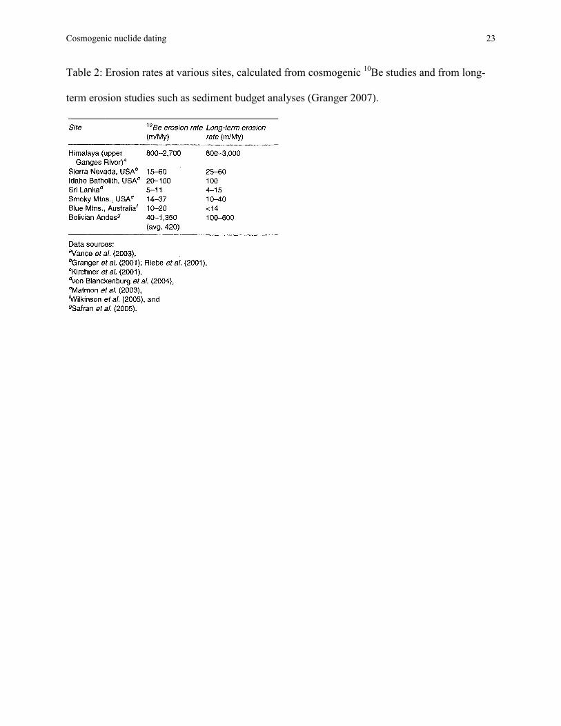
studies can be calibrated, as can soil development rates (Gosse and Phillips 2001). Table 2

summarizes erosion rates calculated from cosmogenic beryllium-10 and their agreement with

more traditional methods like sediment budget calculations and thermochronometry (Granger

2007).

(ii) Landslides

A common application of cosmogenic nuclide dating is in determining the age of

landslide deposits. Assuming that previously buried material was at great enough depth to not

appreciably accumulate cosmogenic nuclides and that there was minimal shifting after the debris

had initially settled, precise dates can be obtained if local nuclide production rates are known

(Ivy-Ochs and Kober 2007). There is some variability in the reliability of samples taken at

different zones throughout a landslide landform, therefore it is ideal if multiple zones are

sampled (Ivy-Ochs and Kober 2007) and ages are averaged.


(iii) Lava flows

Igneous rock of any type can be dated via traditional radiometric techniques like

39Ar/40Ar dating. However, due to the much longer half-lives of isotopes used in these studies,

there is a lower limit to the ages they are able to produce (Ivy-Ochs and Kober 2007). Most

cosmogenic nuclides have much shorter half-lives, and have proven useful in the dating of lava

flows less than 45 thousand years old. Previously the best age indicators of these flows rested

with the radiocarbon dating of charcoal layers, or by making stratigraphic inferences (Ivy-Ochs

and Kober 2007).

Hundreds of lava flows have been dated using cosmogenic nuclides (Gosse 2007).

However, samples must still be taken from the surface of the flow (Ivy-Ochs and Kober 2007).

This is in contrast to traditional radiometric dating techniques for igneous rock.

(iv) Glaciers

Before cosmogenic nuclide dating was fully developed, radiocarbon or stratigraphic

dating sufficed for estimating ages of glacial landforms (Ivy-Ochs and Kober 2007). With

cosmogenic nuclide dating, moraines can be dated to obtain an absolute age of the maximum

extent of a glacier, bringing much greater precision to previous quaternary geology problems.

However, sample selection on a moraine must be done carefully, since moraines are susceptible

to instability and degradation over time (Ivy-Ochs and Kober 2007). It is possible to date a

glacially modified bedrock surface, however the ages returned will likely be imprecise due to

likely shielding by till emplaced shortly after the glacier retreated over the surface (Ivy-Ochs and

Kober 2007).


(v) Fluvial and alluvial landforms

On composite landforms like alluvial fans, boulders dated from across the fan may

indicate a progression of deposition over time (Ivy-Ochs and Kober 2007). By knowing detailed

aggradation rates, researchers can glean insight inter sediment supply variations, base level

changes and slope changes (Ivy-Ochs and Kober 2007).

(vi) Faults

Another application of cosmogenic nuclide dating is in dating fault movements. If a fault

scarp become exposed, or increasingly exposed after a rupture, a series of samples can be taken

along the scarp (Ivy-Ochs and Kober 2007). This will in turn provide a detailed rupture history

of the fault, limited only by erosion and nuclide production rates.

(vii) Archaeology

Cosmogenic nuclide dating is increasing finding use in archaeology as well. Based on

beryllium-10 concentrations, Verri et al. (2005) determined that chert tools found in a cave were

between 200 - 400 thousand years old, and that the tools were quarried from surface pits or

mines more than several metres in depth (Ivy-Ochs and Kober 2007). It is a valuable tool for

archaeologists, and other specific applications may yet be developed.

(E) Conclusion

For the many quaternary geology problems that cosmogenic nuclide dating may be able

to shed light on, there are likely just as many more unexplored applications owing directly to

how young this technique is and the novelty of dating exposed surfaces. Some landforms were

previously very difficult to date if they were younger than 45 thousand years. With cosmogenic


nuclide dating, a lower obtainable minimum age than other mainstream techniques means that

much of the quaternary period can benefit from these techniques. Careful consideration as to

what corrections to make and when are key to obtaining precise dates however, and continued

work on calibration studies should assist past, present and future studies as more refined

calibration curves are obtained. One particular study is currently underway to standardize global

cosmogenic nuclide production rates, the Cosmic-Ray Produced Nuclide Systematics on Earth

Project (CRONUS-Earth). It is expected to be completed in 2010 and should help improve the

precision and convenience of cosmogenic nuclide dating considerably.


(F) References

American Geological Institute. 2008. Definition of “spallation”. [online]. Available from

http://glossary.agiweb.org/dbtw-wpd/exec/dbtwpub.dll?ac=qbe_query&bu=

http://glossary.agiweb.org/dbtw-wpd/glossary/search.htm&tn=glossary_web&qy=

ID%20ct%2040170&mr=10&np=255&rf=results [cited 16 March 2008].

Braucher, R., Benedetti, L., Bourles, D., Brown, E.T., and Chardon, D. 2005. Use on in-situ

produced Be-10 in carbonate rich environments: A first attempt. Geochimica et Cosmochimica

Acta 69(6): 1473-1478.

Desilets, D.M. 2005. Cosmogenic nuclides as a surface exposure dating tool: improved

altitude/latitude scaling factors for production rates. Ph.D. dissertation, Department of Hydrology

and Water Resources, The University of Arizona, Tuscon, Arizona.

Gosse, J.C. 2007. Cosmogenic nuclide dating; overview. In Encyclopedia of Quaternary science.

Edited by S.A. Elias. Elsevier, Amsterdam, Netherlands. pp. 409-411.

Gosse, J.C., and Phillips, F.M. 2001. Terrestrial in situ cosmogenic nuclides: theory and

application. Quaternary Science Reviews, 20: 1475-1560.

Granger, D.E. 2007. Cosmogenic nuclide dating; landscape evolution. In Encyclopedia of

Quaternary science. Edited by S.A. Elias. Elsevier, Amsterdam, Netherlands. pp. 445-452.


Ivy-Ochs, S., and Kober, F. 2007. Cosmogenic nuclide dating; exposure geochronology. In

Encyclopedia of Quaternary science. Edited by S.A. Elias. Elsevier, Amsterdam, Netherlands.

pp. 436-445.

Lal, D. 1958. Investigation of nuclear interactions produced by cosmic rays. Ph.D. thesis,

University of Mumbai, Mumbai.

Lal, D. 1991. Cosmic ray labeling of erosion surfaces: in situ nuclide production rates and

erosion models. Earth and Planetary Science Letters, 104: 424-439.

Lal, D. 2007. Cosmogenic nuclide dating; cosmic ray interactions in minerals. In Encyclopedia

of Quaternary science. Edited by S.A. Elias. Elsevier, Amsterdam, Netherlands. pp. 419-436.

Lal, D., and Peters, B. 1967. Cosmic ray produced radioactivity on the earth. In Handbuch der

Physik. Edited by K. Sitte. Springer, Berlin. pp. 551-612.

Schaefer, J.M., and Lifton, N. 2007. Cosmogenic nuclide dating; methods. In Encyclopedia of

Quaternary science. Edited by S.A. Elias. Elsevier, Amsterdam, Netherlands. pp. 412-419.

Stone, J. 2000. Air pressure and cosmogenic isotope production. Journal of Geophysical

Research, 105(B10): 23753-23759.


Verri, G., Barkai, R., Gopher, A., et al. 2005. Flint procurement strategies in the Late Lower

Paleolithic recorded by in situ produced cosmogenic Be-10 in Tabun and Qesem Caves (Israel).

Journal of Archaeological Science, 32: 207-213.


(G) Tables

Table 1: Production rates of commonly used cosmogenic nuclides, calibrated to sea level and

high lattitude (Schaefer and Lifton 2007).


Table 2: Erosion rates at various sites, calculated from cosmogenic 10Be studies and from long-

term erosion studies such as sediment budget analyses (Granger 2007).


(H) Figures

Figure 1: Depth profiles of saturation equilibrium 10Be concentrations in eroding bedrock

surfaces at sea level and high latitude (Ivy-Ochs and Kober 2007). Increasing erosion rates

obscure the cosmogenic signature.

surface exposure cosmogenic nuclide dating - · pdf fileexposure dating that cosmogenic...

Documents