Surface Estimation, Variable Selection, and the

Nonparametric Oracle Property

Curtis B. Storlie, Howard D. Bondell, Brian J. Reich, and Hao Helen Zhang

Date: March 26, 2009

Abstract

Variable selection for multivariate nonparametric regression is an impor-tant, yet challenging, problem due, in part, to the infinite dimensionality of thefunction space. An ideal selection procedure should be automatic, stable, easyto use, and have desirable asymptotic properties. In particular, we define aselection procedure to be nonparametric oracle (np-oracle) if it consistently se-lects the correct subset of predictors and at the same time estimates the smoothsurface at the optimal nonparametric rate, as the sample size goes to infinity.In this paper, we propose a model selection procedure for nonparametric mod-els, and explore the conditions under which that the new method enjoys theaforementioned properties. Developed in the framework of smoothing splineANOVA, our estimator is obtained via solving a regularization problem witha novel adaptive penalty on the sum of functional component norms. Theo-retical properties of the new estimator are established. Additionally, numeroussimulated and real examples further demonstrate that the new approach sub-stantially outperforms other existing methods in the finite sample setting.

Keywords: Adaptive LASSO, Nonparametric Regression, Regularization Method,Variable Selection, Smoothing Spline ANOVA.

Running title: Adaptive COSSO.

Corresponding Author: Curtis Storlie, storlie@stat.unm.edu

1 Introduction

In this paper, we consider the multiple predictor nonparametric regression model

yi = f(xi) + εi , i = 1, ..., n, where f is the unknown regression function, xi =

(x1,i, ..., xp,i) is a p-dimensional vector of predictors, and the εi’s are independent noise

terms with mean 0 and variances σ2i . Many approaches to this problem have been

proposed, such as kernel regression (Nadaraya 1964 and others) and locally weighted

1

polynomial regression (LOESS), (Cleveland 1979). See Schimek (2000) for a detailed

list of references. When there are multiple predictors, these procedures suffer from the

well known curse of dimensionality. Additive models (GAM’s) (Hastie & Tibshirani

1990) avoid some of the problems with high dimensionality and have been shown to

be quite useful in cases when the true surface is nearly additive. A generalization of

additive modeling is the Smoothing Spline ANOVA (SS-ANOVA) approach (Wahba

1990, Stone, Buja & Hastie 1994, Wahba, Wang, Gu, Klein & Klein 1995, Lin 2000,

and Gu 2002). In SS-ANOVA, the function f is decomposed into several orthogonal

functional components.

We are interested in the variable selection problem in the context of multiple pre-

dictor nonparametric regression. For example, it might be thought that the function

f only depends on a subset of the p predictors. Traditionally this problem has been

solved in a stepwise or best subset type model selection approach. The MARS proce-

dure (Friedman 1991) and variations thereof (Stone, Hansen, Kooperberg & Truong

1997) build an estimate of f by adding and deleting individual basis functions in

a stepwise manner so that the omission of entire variables occurs as a side effect.

However, stepwise variable selection is known to be unstable due to its inherent dis-

creteness (Breiman 1995). COmponent Selection Shrinkage Operator (COSSO; Lin

& Zhang 2006) performs variable selection via continuous shrinkage in SS-ANOVA

models by penalizing the sum of norms of the functional components. Since each of

the components are continuously shrunk towards zero, the resulting estimate is more

stable than in subset or stepwise regression.

What are the desired properties of a variable selection procedure? For the para-

metric linear model Fan & Li (2001) discuss the oracle property. A method is said

to possess the oracle property if it selects the correct subset of predictors with prob-

ability tending to one and estimates the non-zero parameters as efficiently as could

be possible if we knew which variables were uninformative ahead of time. Parametric

2

models with the oracle property include Fan & Li (2001) and Zou (2006). In the con-

text of nonparametric regression, we extend the notion of the oracle property. We say

a nonparametric regression estimator has the nonparametric (np)-oracle property if it

selects the correct subset of predictors with probability tending to one and estimates

the regression surface f at the optimal nonparametric rate.

None of the aforementioned nonparametric regression methods have been demon-

strated to possess the np-oracle property. In particular, COSSO has a tendency to

over-smooth the nonzero functional components in order to set the unimportant func-

tional components to zero. In this paper we propose the adaptive COSSO (ACOSSO)

to alleviate this major stumbling block. The intuition behind the ACOSSO to penal-

ize each component differently so that more flexibility is given to estimate functional

components with more trend and/or curvature, while penalizing unimportant com-

ponents more heavily. Hence it is easier to shrink uninformative components to zero

without much degradation to the overall model fit. This is motivated by the adaptive

LASSO procedure for linear models of Zou (2006). We explore a special case under

which the ACOSSO possesses the np-oracle property. This is the first result of this

type for a nonparametric regression estimator. The practical benefit of possessing

this property is demonstrated on several real and simulated data examples where the

ACOSSO substantially outperforms other existing methods.

In Section 2 we review the necessary literature on smoothing spline ANOVA. The

ACOSSO is introduced in Section 3 and its asymptotic properties are presented in

Section 4. In Section 5 we discuss the computational details of the estimate. Its

superior performance to the COSSO and MARS is demonstrated on simulated data

in Section 6 and real data in Section 7. Section 8 concludes. Proofs are given in an

appendix.

3

2 Smoothing Splines and the COSSO

In this section we review only the necessary concepts of SS-ANOVA needed for de-

velopment. For a more detailed overview of Smoothing Splines and SS-ANOVA see

Wahba (1990), Wahba et al. (1995), Schimek (2000), Gu (2002), and Berlinet &

Thomas-Agnan (2004).

In the smoothing spline literature it is typically assumed that f ∈ F where F

is a reproducing kernel Hilbert space (RKHS). Denote the reproducing kernel (r.k.),

inner product, and norm of F as KF , 〈·, ·〉F , and ‖ · ‖F respectively. Often F is

chosen to contain only functions with a certain degree of smoothness. For example,

functions of one variable are often assumed to belong to the second order Sobolev

space, S2 = {g : g, g′ are absolutely continuous and g′′ ∈ L2[0, 1]}.

Smoothing spline models are usually assumed without loss of generality to be over

x ∈ X = [0, 1]p. In what is known as smoothing spline (SS)-ANOVA, the space F

is constructed by first taking a tensor product of p one dimensional RKHS’s. For

example, let Hj be a RKHS on [0, 1] such that Hj = {1}⊕Hj where {1} is the RKHS

consisting of only the constant functions and Hj is the RKHS consisting of functions

fj ∈ Hj such that < fj, 1 >Hj= 0. The space F can be taken to be the tensor product

of the Hj, j = 1, . . . , p which can be written as

F =

p⊗j=1

Hj = {1} ⊕

{p⊕

j=1

Hj

}⊕

{⊕j<k

(Hj ⊗ Hk)

}⊕ · · · . (1)

The right side of the above equation has decomposed F into the constant space,

the main effect spaces, the two-way interaction spaces, etc. which gives rise to the

name SS-ANOVA. Typically (1) is truncated so that F includes only lower order

interactions for better estimation and ease of interpretation. Regardless of the order

of the interactions involved, we see that the space F can be written in general as

F = {1} ⊕

{q⊕

j=1

Fj

}(2)

4

where {1},F1 . . .Fq is an orthogonal decomposition of the space and each of the

Fj is itself a RKHS. In this presentation we will focus on two special cases, the

additive model f(x) = b +∑p

j=1 fj(xj) and the two-way interaction model f(x) =

b +∑p

j=1 fj(xj) +∑p

j<k fjk(xj, xk), where b ∈ {1}, fj ∈ Hj and fjk ∈ Hj ⊗ Hk.

A traditional smoothing spline type estimate, f , is given by the function f ∈ F

that minimizes1

n

n∑i=1

(yi − f(xi))2 + λ0

q∑j=1

1

θj

‖P jf‖2F , (3)

where P jf is the orthogonal projection of f onto Fj, j = 1, . . . , q which form an

orthogonal partition of the space as in (2). We will use the convention 0/0 = 0 so

that when θj = 0 the minimizer satisfies ‖P jf‖F = 0.

The COSSO (Lin & Zhang 2006) penalizes on the sum of the norms instead of

the squared norms as in (3) and hence achieves sparse solutions (e.g. some of the

functional components are estimated to be exactly zero). Specifically, the COSSO

estimate, f , is given by the function f ∈ F that minimizes

1

n

n∑i=1

(yi − f(xi))2 + λ

q∑j=1

‖P jf‖F . (4)

In Lin & Zhang (2006), F was formed using S2 with squared norm

‖f‖2 =

(∫ 1

0

f(x)dx

)2

+

(∫ 1

0

f ′(x)dx

)2

+

∫ 1

0

(f ′′(x))2dx (5)

for each of the Hj of (1). The reproducing kernel can be found in Wahba (1990).

3 An Adaptive Proposal

Although the COSSO is a significant improvement over classical stepwise procedures,

it tends to oversmooth functional components. This seemingly prevents COSSO from

achieving a nonparametric version of the oracle property (defined in Section 4). To

alleviate this problem, we propose an adaptive approach. The proposed adaptive

5

COSSO uses individually weighted norms to smooth each of the components. Specif-

ically we select as our estimate the function f ∈ F that minimizes

1

n

n∑i=1

(yi − f(xi))2 + λ

q∑j=1

wj‖P jf‖F . (6)

where the 0 < wj ≤ ∞ are weights that can depend on an initial estimate of f which

we denote f . For example we could initially estimate f via the traditional smoothing

spline of (3) with all θj = 1 and λ0 chosen by the generalized cross validation (GCV )

criterion (Craven & Wahba 1979). Note that there is only one tuning parameter, λ,

in (6). The wj’s are not tuning parameters like the θj’s in (3), rather they are weights

to be estimated from the data in a manner described below.

3.1 Choosing the Adaptive Weights, wj

Given an initial estimate f , we wish to construct wj’s so that the prominent functional

components enjoy the benefit of a smaller penalty relative to less important functional

components. In contrast to the linear model, there is no single coefficient, or set of

coefficients, to measure importance of a variable. One possible scheme would be to

make use of the L2 norm of P j f given by ‖P j f‖L2 = (∫X (P j f(x))2dx)1/2. For a

reasonable initial estimator, this quantity will be a consistent estimate of ‖P jf‖2L2

which is often used to quantify the importance of functional components. This would

suggest using

wj = ‖P j f‖−γL2

. (7)

In Section 4, the use of these weights results in favorable theoretical properties.

There are other reasonable possibilities one could consider for the wj’s. In fact at

first glance, as an extension of the adaptive LASSO for linear models, it may seem

more natural to make use of an estimate of the RKHS norm used in the COSSO

penalty and set wj = ‖P j f‖−γF . However, the use of these weights is not recom-

mended because they do not provide an estimator with sound theoretical properties.

6

Consider for example building an additive model using RKHS’s with norm given by

(5). Then this wj is essentially requiring estimation of the functionals∫ 1

0(f ′′j (xj))

2dxj

which is known to be a harder problem (requiring more smoothness assumptions) than

estimating∫ 1

0f 2

j (x)dx (Efromovich & Samarov 2000). In fact, using wj = ‖P j f‖−γF

instead of (7) would at the very least require stronger smoothness assumptions about

the underlying function f in Section 4 to achieve asymptotically correct variable selec-

tion. Because of this and the results of preliminary empirical studies we recommend

the use of the weights in (7) instead.

4 Asymptotic Properties

In this section we demonstrate the desirable asymptotic properties of the ACOSSO. In

particular, we show that the ACOSSO possesses a nonparametric analog of the oracle

property. This result is the first of its type for nonparametric surface estimation.

Throughout this section we assume the true regression model is yi = f0(xi) +

εi, i = 1, . . . , n . The regression function f0 ∈ F is additive in the predictors so

that F = {1} ⊕ F1 ⊕ · · · ⊕ Fp where each Fj is a space of functions corresponding

to xj. We assume that εi are independent with Eεi = 0 and are uniformly sub-

Gaussian. Following van de Geer (2000), we define a sequence of random variables to

be uniformly sub-Gaussian if there exists some K > 0 and C > 0 such that

supn

maxi=1,...,n

E[exp(ε2i /K)] ≤ C. (8)

Let S2 denote the RKHS of second order Sobolev space endowed with the norm

in (5) with S2 = {1} ⊕ S2. Also, define the squared norm of a function at the design

points as ‖f‖2n = 1/n

∑ni=1 f 2(xi). Let U be the set of indexes for all uninformative

functional components in the model f0 = b +∑p

j=1 P jf0, j = 1, . . . , p. That is

U = {j : P jf0 ≡ 0}.

7

Theorem 1 below states the convergence rate of ACOSSO when used to estimate

an additive model. Corollary 1 following Theorem 1 states that the weights given by

(7) lead to an estimator with optimal convergence rate of n−2/5. We sometimes write

wj and λ as wj,n and λn respectively to explicitly denote the dependence on n. We

also use the notation Xn ∼ Yn to mean Xn/Yn = Op(1) and Yn/Xn = Op(1) for some

sequences Xn and Yn. The proofs of Theorem 1 and the other results in this section

are deferred to the appendix.

Theorem 1. (Convergence Rate) Assume that f0 ∈ F = {1}⊕S21⊕· · ·⊕S2

p where

S2j is the space S2 corresponding to the jth input variable, xj. Also assume that εi

are independent and satisfy (8). Consider the ACOSSO estimate, f , defined in (6).

Suppose that w−1j,n = Op(1) for j = 1, . . . , p and further that wj,n = Op(1) for j ∈ U c.

Also assume that λ−1n = Op(n

4/5). If

(i) P jf0 6= 0 for some j, then ‖f−f0‖n = Op(λ1/2w

1/2∗,n ) where w∗,n = min{w1,n, . . . , wp,n}.

(ii) P jf0 = 0 for all j, then ‖f − f0‖n = Op(max{n−1/2, n−2/3λ−1/3w−1/3∗,n }).

Corollary 1. (Optimal Convergence of ACOSSO) Assume that f0 ∈ F =

{1}⊕S21⊕· · ·⊕S2

p and that εi are independent and satisfy (8). Consider the ACOSSO

estimate, f , with weights, wj,n = ‖P j f‖−γL2

, for f given by the traditional smoothing

spline (3) with θ = 1p and λ0,n ∼ n−4/5. If γ > 3/4 and λn ∼ n−4/5, then ‖f−f0‖n =

Op(n−2/5) if P jf0 6= 0 for some j and ‖f − f0‖n = Op(n

−1/2) otherwise.

We now turn to discuss the attractive properties of the ACOSSO in terms of model

selection. In Theorem 2 and Corollary 2 we will consider functions in the second order

Sobolev space of periodic functions denoted S2per where S2

per = {1} ⊕ S2per. We also

assume that the observations come from a tensor product design. That is, the design

points are {x1,i1 , x2,i2 , . . . , xp,ip}m p

ij=1 j=1where xj,k = k/m, k = 1, . . . ,m, j = 1, . . . , p.

8

Therefore the total sample size is n = mp. These assumptions were also used by Lin

& Zhang (2006) to examine the model selection properties of the COSSO.

Theorem 2. (Selection Consistency) Assume a tensor product design and f0 ∈

F = {1} ⊕ S2per,1 ⊕ · · · ⊕ S2

per,p where S2per,j is the space S2

per corresponding to the jth

input variable, xj. Also assume that εi are independent and satisfy (8). The ACOSSO

estimate f will be such that P j f ≡ 0 for all j ∈ U with probability tending to one if

and only if nw2j,nλ

2n

p→ ∞ as n →∞ for all j ∈ U .

We will say a nonparametric regression estimator, f , has the nonparametric (np)-

oracle property if ‖f − f0‖n → 0 at the optimal rate while also setting P j f ≡ 0

for all j ∈ U with probability tending to one. This means that the error associated

with surface estimation has the same order as that for any other optimal estimator.

One could also define a strong np-oracle property which would require asymptotically

correct variable selection and the error being asymptotically the same as an oracle

estimator (an estimator where the correct variables were known in advance). That

is, to possess the strong np-oracle property, the proposed estimator must match the

constant as well as the rate of an oracle estimator. The strong np-oracle definition

is slightly ambiguous however, as one must specify what estimator should be used

as the oracle estimator for comparison (e.g. smoothing spline with one λ, smoothing

spline with differing λj’s, etc.). The weaker version of the np-oracle property, which

was stated first, avoids this dilemma. The corollary below states that the ACOSSO

with weights given by (7) has the np-oracle property.

Corollary 2. (Nonparametric Oracle Property) Assume a tensor product de-

sign and f0 ∈ F where F = {1}⊕ S2per,1⊕ · · ·⊕ S2

per,p and that εi are independent and

satisfy (8). Define weights, wj,n = ‖P j f‖−γL2

, for f given by the traditional smoothing

spline with λ0 ∼ n−4/5, and γ > 3/4. If also λn ∼ n−4/5, then the ACOSSO estimator

has the np-oracle property.

9

Remark 1: The derivation of the variable selection properties of adaptive COSSO

requires detailed investigation on the eigen-properties of the reproducing kernel, which

is generally intractable. However, Theorem 2 and the Corollary 2 assume that f

belongs to the class of periodic functions while x is a tensor product design. This

makes the derivation more tangible, since the eigenfunctions and eigenvalues of the

associated reproducing kernel have a particularly simple form. Results for this specific

design are often instructive for general cases, as suggested in Wahba (1990). We

conjecture that the selection consistency of the adaptive COSSO also holds more

generally, and this is also supported by numerical results in Section 6. The derivation

of variable selection properties in the general case is a technically difficult problem

which is worthy of future investigation. Neither the tensor product design nor the

periodic functions assumptions are required for establishing the MSE consistency of

the adaptive COSSO estimator in Theorem 1 and Corollary 1.

Remark 2: The COSSO (which is the ACOSSO with wj,n = 1 for all j and n)

does not appear to enjoy the np-oracle property. Notice that by Theorem 2, λn

must go to zero slower than n−1/2 in order to achieve asymptotically correct variable

selection. However, even if λn is as small as λn = n−1/2, Theorem 1 implies that the

convergence rate is Op(n−1/4) which is not optimal. These results are not surprising

given that the linear model can be obtained as a special case of ACOSSO by using

F = {f : f = β0 +∑p

j=1 βj(xj−1/2)}. For this F the COSSO reduces to the LASSO

which is known to be unable to achieve the oracle property (Knight & Fu 2000, Zou

2006). In contrast, the ACOSSO reduces to the adaptive LASSO (Zou 2006) which

is well known to achieve the oracle property.

Remark 3: The distribution of the error terms εi in Theorems 1 and 2 need only be

independent with sub-Gaussian tails (8). The common assumption that εiiid∼ N (0, σ2)

satisfies (8). But, the distributions need not be Gaussian and further need not even

be the same for each of the εi. In particular, this allows for heteroskedastic errors.

10

Remark 4: Theorems 1 and 2 are assuming an additive model, in which case

functional component selection is equivalent to variable selection. In higher order

interaction models, the main effect for xj and all of the interaction functional com-

ponents involving xj must be set to zero in order to eliminate xj from the model and

achieve true variable selection. Thus, in some other areas of the paper, when interac-

tions are involved, we use the term variable selection to refer to functional component

selection.

5 Computation

Since the ACOSSO in (6) may be viewed as the COSSO in (4) with an “adaptive”

RKHS, the computation proceeds in a similar manner as that for the COSSO. We

first present an equivalent formulation of the ACOSSO, then describe how to minimize

this equivalent formulation for a fixed value of the tuning parameter. Discussion of

tuning parameter selection is delayed until Section 5.3.

5.1 Equivalent Formulation

Consider the problem of finding θ = (θ1, . . . , θq)′ and f ∈ F to minimize

1

n

n∑i=1

[yi − f(xi)]2 + λ0

q∑j=1

θ−1j w2−ϑ

j ‖P jf‖2F + λ1

q∑j=1

wϑj θj, subject to θj ≥ 0 ∀j, (9)

where 0 ≤ ϑ ≤ 2, λ0 > 0 is a fixed constant, and λ1 > 0 is a smoothing parameter.

The following Lemma says that the above optimization problem is equivalent to (6).

This has important implications for computation since (9) is easier to solve.

Lemma 1. Set λ1 = λ2/(4λ0). (i) If f minimizes (6), set θj = λ1/20 λ

−1/21 w1−ϑ

j ‖P j f‖F ,

j = 1, . . . , q, then the pair (θ, f) minimizes (9). (ii) On the other hand, if a pair (θ, f)

minimizes (9), then f minimizes (6).

11

5.2 Computational Algorithm

The equivalent form in (9) gives a class of equivalent problems for ϑ ∈ [0, 2]. For

simplicity we will consider the case ϑ = 0 since the ACOSSO can be then viewed

as having the same equivalent form as the COSSO with an adaptive RKHS. For a

given value of θ = (θ1, . . . , θq)′, the minimizer of (9) is the smoothing spline of (3)

with θj replaced by w−2j θj. Hence it is known (Wahba 1990 for example) that the

solution has the form f(x) = b +∑n

i=1 ciKw,θ(x, xi) where c ∈ <n, b ∈ < and

Kw,θ =∑q

j=1(θj/w2j )KFj

, with Fj corresponding to the decomposition in (2).

Let Kj be the n × n matrix {KFj(xi, xj)}n

i,j=1 and let 1n be the column vector

consisting of n ones. Then write the vector f = (f(x1), . . . , f(xn))′ as f = b1n +

(∑q

j=1(θj/w2j )Kj)c, y = (y1, . . . , yn)′ and define ‖v‖2

n = 1/n∑n

i=1 v2i for a vector v

of length n and y = (y1, . . . , yn)′. Now, for fixed θ, minimizing (9) is equivalent to

minb,c

1

n

∥∥∥∥∥y − b1n −q∑

j=1

θjw−2j Kjc

∥∥∥∥∥2

n

+ λ0

q∑j=1

θjw−2j c′Kjc

(10)

which is just the traditional smoothing spline problem in Wahba (1990). On the other

hand if b and c were fixed, the θ that minimizes (9) is the same as the solution to

minθ

{‖z −Gθ‖2

n + nλ1

q∑j=1

θj

}, subject to θj ≥ 0 ∀j, (11)

where gj = w−2j Kjc, G is the n × p matrix with the jth column being gj and

z = y − b1n − (n/2)λ0c. Notice that (11) is equivalent to

minθ‖z −Gθ‖2

n subject to θj ≥ 0 ∀j and

q∑j=1

θj ≤ M, (12)

for some M > 0. The formulation in (12) is a quadratic programming problem

with linear constraints for which there exists many algorithms to find the solution

(see Goldfarb & Idnani 1982 for example). A reasonable scheme is then to iterate

between (10) and (12). In each iteration (9) is decreased. We have observed that

12

after the second iteration the change between iterations is small and decreases slowly.

5.3 Selecting the Tuning Parameter

In (9) there is really only one tuning parameter, λ1 or equivalently M of (12). Chang-

ing the value of λ0 will only scale shift the value of M being used so λ0 can be fixed

at any positive value. Therefore, we choose to initially fix θ = 1q and find λ0 to

minimize the GCV score of the smoothing spline problem in (10). This has the effect

of placing the θj’s on a scale so that M roughly translates into the number of non-zero

components. Hence, it seems reasonable to tune M on [0, 2q] for example.

We will use 5-fold cross validation (5CV ) in the examples of the subsequent sec-

tions to tune M . However, we also found that the BIC criterion (Schwarz 1978) was

quite useful for selecting M . We approximate the effective degrees of freedom, ν, by

ν = tr(S) where S is the weight matrix corresponding to the smoothing spline fit

with θ = θ. This type of approximation gives an under-estimate of the actual df ,

but has been demonstrated to be useful (Tibshirani 1996). We have found that the

ACOSSO with 5CV tends to over select non-zero components just as Zou, Hastie

& Tibshirani (2007) found that AIC-type criteria over select non-zero coefficients in

the LASSO. They recommend using BIC with the LASSO when the goal is variable

selection as do we for the ACOSSO.

6 Simulated Data Results

In this section we study the empirical performance of the ACOSSO estimate and

compare it to several other existing methods. We display the results of four different

versions of the ACOSSO. All versions use weights wj given by (7) with γ = 2 since we

found that γ = 2 produced the best overall results among γ ∈ {1.0, 1.5, 2.0, 2.5, 3.0}.

The initial estimate, f , is either the traditional smoothing spline or the COSSO with

13

λ selected by GCV . We also use either 5CV or BIC to tune M . Hence the four

versions of ACOSSO are ACOSSO-5CV-T, ACOSSO-5CV-C, ACOSSO-BIC-T, and

ACOSSO-BIC-C where (-T) and (-C) stand for using the traditional smoothing spline

and COSSO respectively for the initial estimate.

We include the methods COSSO, MARS, stepwise GAM, Random Forest (Breiman

2001), and the Gradient Boosting Method (GBM) (Friedman 2001). The tuning pa-

rameter for COSSO is chosen via 5CV . To fit MARS models we have used the

’polymars’ procedure in the R-package ’polspline’. Stepwise GAM, Random Forest,

and GBM fits were obtained using the R-packages ’gam’, ’randomForest’, and ’gbm’

respectively. All input parameters for these methods such as gcv for MARS, n.trees

for GBM, etc. were appropriately set to give the best results on these examples.

Note that Random Forest and GBM are both black box prediction machines.

That is they produce function estimates that are difficult to interpret and they are

not intended for variable selection. They are however well known for making accurate

predictions. Thus, they are included here to demonstrate the utility of the ACOSSO

even in situations where prediction is the only goal.

We also include the results of the traditional smoothing spline of (3) when fit with

only the informative variables. That is, we set θj = 0 if P jf = 0 and θj = 1 otherwise,

then choose λ0 by GCV. This will be referred to as the ORACLE estimator. Notice

that the ORACLE estimator is only available in simulations where we know ahead

of time which variables are informative. Though the ORACLE cannot be used in

practice, it is useful to display its results here because it gives us a baseline for the

best estimation risk we could hope to achieve with the other methods.

Performance is measured in terms of estimation risk and model selection. Specifi-

cally, the variables defined in Table 1 will be used to compare the different methods.

We first present a very simple example to highlight the benefit of using the ACOSSO.

We then repeat the same examples used in the COSSO paper to offer a direct compar-

14

R is a monte carlo estimate of the estimation risk, R(f) = E{f(X) −f(X)}2. Specifically, let the integrated squared error for a fixed estimatef be given by ISE = EX{f(X)−f(X)}2. The ISE is calculated for eachrealization via a monte carlo integration with 1000 points. The quantityR is then the average of the ISE values over the N = 100 realizations.

α is a monte carlo estimate of the type I error rate averaged over all of theuninformative functional components. Specifically, let αj be the propor-tion of realizations that P j f 6= 0, j = 1, . . . , q. Then α = 1/|U |

∑j∈U αj

where U = {j : P jf ≡ 0} and |U | is the number of elements in U .1 − β is a monte carlo estimate of the variable selection power averaged over

all of the informative functional components. Specifically, let βj bethe proportion of realizations that P j f = 0, j = 1, . . . , q. Then β =1/|U c|

∑j∈Uc βj where U c is the complement of U .

model size is the number of functional components included in the model avergedover the N = 100 realizations.

Table 1: Definitions of the variables R, α, 1− β, and model size used to summarizethe results of the simulations.

ison on examples where the COSSO is known to perform well. The only difference is

that we have increased the noise level to make these problems a bit more challenging.

Example 1. The following four functions on [0, 1] are used as building blocks of

regression functions in the following simulations:

g1(t) = t; g2(t) = (2t− 1)2; g3(t) =sin(2πt)

2− sin(2πt);

g4(t) = 0.1 sin(2πt)+ 0.2 cos(2πt)+ 0.3 sin2(2πt)+ 0.4 cos3(2πt)+ 0.5 sin3(2πt). (13)

We consider the same two distributional families for the input vector X as in Lin &

Zhang (2006).

Compound Symmetry: For an input X = (X1, . . . , Xp), let Xj = (Wj+tU)/(1+t), j =

1, . . . , p, where W1, . . . ,Wp and U are iid from Unif(0, 1). Thus, Corr(Xj, Xk) =

t2/(1 + t2) for j 6= k. The uniform distribution design corresponds to the case t = 0.

(trimmed) AR(1): Let W1, . . . ,Wd be iid N (0, 1), and let X1 = W1, Xj = ρXj−1 +

(1− ρ2)1/2Wj , j = 2, . . . , p. Then trim Xj in [−2.5, 2.5] and scale to [0, 1].

15

In this example, we let X ∈ <10. We observe n = 100 observations from the

model y = f(X) + ε where the underlying regression function is additive,

f(x) = 5g1(x1) + 3g2(x2) + 4g3(x3) + 6g4(x4)

and εiid∼ N (0, 3.03). Therefore X5, . . . , X10 are uninformative. We first consider the

case where X is uniform in [0, 1]10 in which case the signal to noise ratio (SNR) is

3:1 (here we have adopted the variance definition for signal to noise ratio, SNR =

[Var(f(X))]/σ2). For comparison, the variances of the functional components are

Var{5g1(X1)} = 2.08, Var{3g2(X2)} = 0.80, Var{4g3(X3)} = 3.30 and Var{6g4(X4)} =

9.45.

For the purposes of estimation in the methods ACOSSO, COSSO, MARS, and

GBM, we restrict f to be a strictly additive function. The Random Forest function

however does not have an option for this. Hence there are 10 functional components

that are considered for inclusion in the ACOSSO model. Figure 1 gives plots of y

versus the the first four variables x1, . . . , x4 along with the true P jf component curves

for a realization from Example 1. The true component curves, j = 1, . . . , 4, along

with the estimates given by ACOSSO-5CV-T and COSSO are then shown in Figure 2

without the data for added clarity. Notice that the ACOSSO captures more of the

features of the P 3f component and particularly the P 4f component since the reduced

penalty on these components allows it more curvature. In addition, since the weights

more easily allow for curvature on components that need it, M does not need to be

large (relatively) to allow a good fit to components like P 3f and P 4f . This has the

effect that that components with less curvature, like the straight line P 1f , can also

estimated more accurately by ACOSSO than by COSSO, as seen in Figure 2.

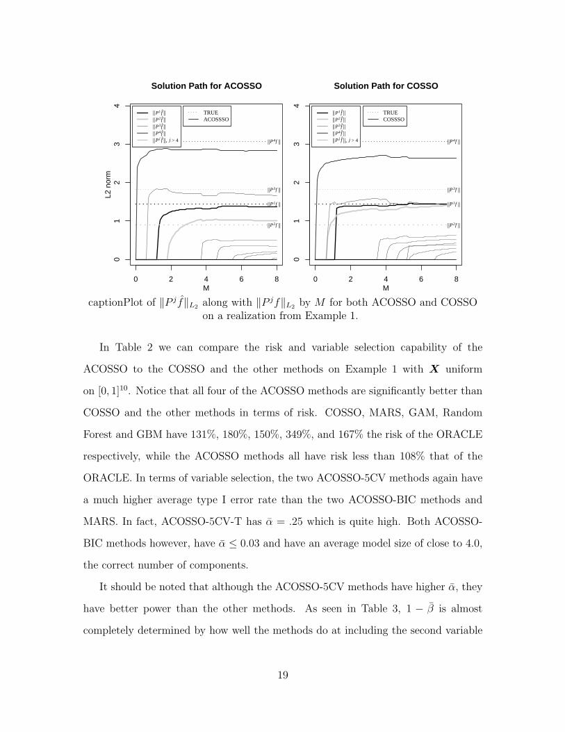
Figure 6 shows how the magnitudes of the estimated components change with the

tuning parameter M for both the COSSO and ACOSSO for the above realization. The

magnitudes of the estimated components are measured by their L2 norm ‖P j f‖L2 .

16

●

●

●

●

●

●●

●

●

●●

●

●

●

●

●

●

●

●

●

●

●

● ●

●

●

●

●

●

●

●

●

●

●

●

●

●

●

●

●

●

●●

●●

●

●

●

●

●

●

●

●●

●●

●

●

●

●

●

●

●

●

●

● ●

●

●

●

●●

●

●

●

●

●

●●

●●

●

●

●

●

●

●●

●

●

●

●

●

●

●

●

●●

●

●

0.0 0.2 0.4 0.6 0.8 1.0

−10

−5

05

10

y

X 1

●

●

●

●

●

●●

●

●

●●

●

●

●

●

●

●

●

●

●

●

●

● ●

●

●

●

●

●

●

●

●

●

●

●

●

●

●

●

●

●

● ●

● ●

●

●

●

●

●

●

●

●●

● ●

●

●

●

●

●

●

●

●

●

●●

●

●

●

●●

●

●

●

●

●

●●

●●

●

●

●

●

●

●●

●

●

●

●

●

●

●

●

●●

●

●

0.0 0.2 0.4 0.6 0.8 1.0

−10

−5

05

10

y

X 2

●

●

●

●

●

●●

●

●

●●

●

●

●

●

●

●

●

●

●

●

●

● ●

●

●

●

●

●

●

●

●

●

●

●

●

●

●

●

●

●

●●

●●

●

●

●

●

●

●

●

●●

●●

●

●

●

●

●

●

●

●

●

● ●

●

●

●

●●

●

●

●

●

●

●●

●●

●

●

●

●

●

●●

●

●

●

●

●

●

●

●

●●

●

●

0.0 0.2 0.4 0.6 0.8 1.0

−10

−5

05

10

y

X 3

●

●

●

●

●

●●

●

●

●●

●

●

●

●

●

●

●

●

●

●

●

●●

●

●

●

●

●

●

●

●

●

●

●

●

●

●

●

●

●

●●

●●

●

●

●

●

●

●

●

●●

●●

●

●

●

●

●

●

●

●

●

●●

●

●

●

●●

●

●

●

●

●

●●

●●

●

●

●

●

●

●●

●

●

●

●

●

●

●

●

● ●

●

●

0.0 0.2 0.4 0.6 0.8 1.0

−10

−5

05

10

y

X 4

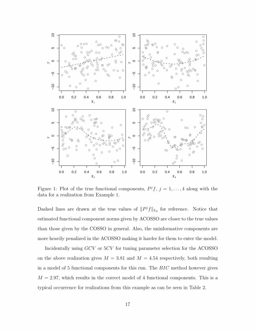
Figure 1: Plot of the true functional components, P jf , j = 1, . . . , 4 along with thedata for a realization from Example 1.

Dashed lines are drawn at the true values of ‖P jf‖L2 for reference. Notice that

estimated functional component norms given by ACOSSO are closer to the true values

than those given by the COSSO in general. Also, the uninformative components are

more heavily penalized in the ACOSSO making it harder for them to enter the model.

Incidentally using GCV or 5CV for tuning parameter selection for the ACOSSO

on the above realization gives M = 3.81 and M = 4.54 respectively, both resulting

in a model of 5 functional components for this run. The BIC method however gives

M = 2.97, which results in the correct model of 4 functional components. This is a

typical occurrence for realizations from this example as can be seen in Table 2.

17

0.0 0.2 0.4 0.6 0.8 1.0

−2

−1

01

23

TRUEACOSSOCOSSO

X 1

P

f 1

0.0 0.2 0.4 0.6 0.8 1.0

−1

01

23

X 2

P

f 2

0.0 0.2 0.4 0.6 0.8 1.0

−2

−1

01

23

X 3

P

f 3

0.0 0.2 0.4 0.6 0.8 1.0

−4

−2

02

4

X 4

P

f 4

Figure 2: Plot of P jf , j = 1, . . . , 4 along with their estimates given by ACOSSO,COSSO, and MARS for a realization from Example 1.

R α 1− β model sizeACOSSO-5CV-T 1.204 (0.042) 0.252 (0.034) 0.972 (0.008) 5.4 (0.21)ACOSSO-5CV-C 1.186 (0.048) 0.117 (0.017) 0.978 (0.007) 4.6 (0.11)ACOSSO-BIC-T 1.257 (0.048) 0.032 (0.008) 0.912 (0.012) 3.8 (0.08)ACOSSO-BIC-C 1.246 (0.064) 0.018 (0.006) 0.908 (0.014) 3.7 (0.07)

COSSO 1.523 (0.058) 0.095 (0.023) 0.935 (0.012) 4.3 (0.15)MARS 2.057 (0.064) 0.050 (0.010) 0.848 (0.013) 3.7 (0.08)GAM 1.743 (0.053) 0.197 (0.019) 0.805 (0.011) 4.4 (0.13)

Random Forest 4.050 (0.062) NA NA 10.0 (0.00)GBM 1.935 (0.039) NA NA 10.0 (0.00)

ORACLE 1.160 (0.034) 0.000 (0.000) 1.000 (0.000) 4.0 (0.00)

Table 2: Results of 100 Realizations from Example 1 in the Uniform Case. Thestandard error for each of the summary statistics is given in parantheses.

18

0 2 4 6 8

01

23

4

|| ||P f1

|| ||P f2

|| ||P f3

|| ||P f4

TRUEACOSSSO

|| |||| |||| |||| |||| ||,

P f1

P f2

P f3

P f4

P fj j > 4

Solution Path for ACOSSO

M

L2 n

orm

0 2 4 6 8

01

23

4

|| ||P f1

|| ||P f2

|| ||P f3

|| ||P f4

TRUECOSSSO

|| |||| |||| |||| |||| ||,

P f1

P f2

P f3

P f4

P fj j > 4

Solution Path for COSSO

M

captionPlot of ‖P j f‖L2 along with ‖P jf‖L2 by M for both ACOSSO and COSSOon a realization from Example 1.

In Table 2 we can compare the risk and variable selection capability of the

ACOSSO to the COSSO and the other methods on Example 1 with X uniform

on [0, 1]10. Notice that all four of the ACOSSO methods are significantly better than

COSSO and the other methods in terms of risk. COSSO, MARS, GAM, Random

Forest and GBM have 131%, 180%, 150%, 349%, and 167% the risk of the ORACLE

respectively, while the ACOSSO methods all have risk less than 108% that of the

ORACLE. In terms of variable selection, the two ACOSSO-5CV methods again have

a much higher average type I error rate than the two ACOSSO-BIC methods and

MARS. In fact, ACOSSO-5CV-T has α = .25 which is quite high. Both ACOSSO-

BIC methods however, have α ≤ 0.03 and have an average model size of close to 4.0,

the correct number of components.

It should be noted that although the ACOSSO-5CV methods have higher α, they

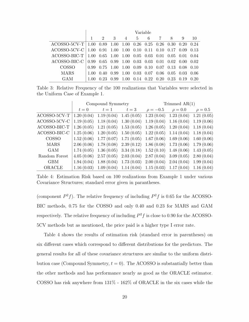
have better power than the other methods. As seen in Table 3, 1 − β is almost

completely determined by how well the methods do at including the second variable

19

Variable1 2 3 4 5 6 7 8 9 10

ACOSSO-5CV-T 1.00 0.89 1.00 1.00 0.26 0.25 0.26 0.30 0.20 0.24ACOSSO-5CV-C 1.00 0.91 1.00 1.00 0.10 0.11 0.10 0.17 0.09 0.13ACOSSO-BIC-T 1.00 0.65 1.00 1.00 0.05 0.03 0.01 0.05 0.01 0.04ACOSSO-BIC-C 0.99 0.65 0.99 1.00 0.03 0.03 0.01 0.02 0.00 0.02

COSSO 0.99 0.75 1.00 1.00 0.09 0.10 0.07 0.13 0.08 0.10MARS 1.00 0.40 0.99 1.00 0.03 0.07 0.06 0.05 0.03 0.06GAM 1.00 0.23 0.99 1.00 0.14 0.22 0.20 0.23 0.19 0.20

Table 3: Relative Frequency of the 100 realizations that Variables were selected inthe Uniform Case of Example 1.

Compound Symmetry Trimmed AR(1)t = 0 t = 1 t = 3 ρ = −0.5 ρ = 0.0 ρ = 0.5

ACOSSO-5CV-T 1.20 (0.04) 1.19 (0.04) 1.45 (0.05) 1.23 (0.04) 1.23 (0.04) 1.21 (0.05)ACOSSO-5CV-C 1.19 (0.05) 1.18 (0.04) 1.30 (0.04) 1.19 (0.04) 1.16 (0.04) 1.19 (0.06)ACOSSO-BIC-T 1.26 (0.05) 1.21 (0.05) 1.53 (0.05) 1.26 (0.05) 1.20 (0.04) 1.18 (0.04)ACOSSO-BIC-C 1.25 (0.06) 1.20 (0.05) 1.50 (0.05) 1.22 (0.05) 1.14 (0.04) 1.18 (0.04)

COSSO 1.52 (0.06) 1.77 (0.07) 1.71 (0.05) 1.67 (0.06) 1.69 (0.06) 1.60 (0.06)MARS 2.06 (0.06) 1.78 (0.08) 2.39 (0.12) 1.86 (0.08) 1.73 (0.06) 1.79 (0.06)GAM 1.74 (0.05) 1.36 (0.05) 3.34 (0.18) 1.52 (0.10) 1.48 (0.06) 1.43 (0.05)

Random Forest 4.05 (0.06) 2.57 (0.05) 2.03 (0.04) 2.87 (0.04) 3.09 (0.05) 2.80 (0.04)GBM 1.94 (0.04) 1.88 (0.04) 1.73 (0.03) 2.00 (0.04) 2.04 (0.04) 1.99 (0.04)

ORACLE 1.16 (0.03) 1.09 (0.04) 1.14 (0.04) 1.15 (0.03) 1.17 (0.04) 1.16 (0.04)

Table 4: Estimation Risk based on 100 realizations from Example 1 under variousCovariance Structures; standard error given in parantheses.

(component P 2f). The relative frequency of including P 2f is 0.65 for the ACOSSO-

BIC methods, 0.75 for the COSSO and only 0.40 and 0.23 for MARS and GAM

respectively. The relative frequency of including P 2f is close to 0.90 for the ACOSSO-

5CV methods but as mentioned, the price paid is a higher type I error rate.

Table 4 shows the results of estimation risk (standard error in parentheses) on

six different cases which correspond to different distributions for the predictors. The

general results for all of these covariance structures are similar to the uniform distri-

bution case (Compound Symmetry, t = 0). The ACOSSO is substantially better than

the other methods and has performance nearly as good as the ORACLE estimator.

COSSO has risk anywhere from 131% - 162% of ORACLE in the six cases while the

20

Compound Symmetry Trimmed AR(1)t = 0 t = 1 t = 3 ρ = −0.5 ρ = 0.0 ρ = 0.5

ACOSSO-5CV-T 0.41 (0.01) 0.41 (0.01) 0.52 (0.01) 0.40 (0.01) 0.40 (0.01) 0.40 (0.01)ACOSSO-5CV-C 0.42 (0.01) 0.40 (0.01) 0.43 (0.01) 0.40 (0.01) 0.40 (0.01) 0.40 (0.01)ACOSSO-BIC-T 0.42 (0.01) 0.41 (0.01) 0.60 (0.02) 0.42 (0.01) 0.39 (0.01) 0.42 (0.01)ACOSSO-BIC-C 0.42 (0.01) 0.42 (0.01) 0.47 (0.01) 0.45 (0.02) 0.39 (0.01) 0.43 (0.01)

COSSO 0.48 (0.01) 0.60 (0.01) 0.54 (0.01) 0.60 (0.02) 0.57 (0.01) 0.57 (0.01)MARS 0.97 (0.02) 0.66 (0.01) 1.05 (0.02) 0.64 (0.01) 0.62 (0.01) 0.64 (0.01)GAM 0.49 (0.01) 0.52 (0.01) 0.50 (0.01) 0.52 (0.01) 0.52 (0.01) 0.52 (0.01)

Random Forest 1.86 (0.01) 1.50 (0.01) 0.76 (0.00) 1.26 (0.01) 1.19 (0.01) 1.25 (0.01)GBM 0.73 (0.01) 0.52 (0.01) 0.47 (0.00) 0.58 (0.01) 0.58 (0.01) 0.57 (0.01)

ORACLE 0.30 (0.00) 0.28 (0.00) 0.27 (0.00) 0.29 (0.00) 0.29 (0.01) 0.29 (0.01)

Table 5: Estimation Risk based on 100 realizations from Example 2 under variousCovariance Structures; standard error given in parantheses.

ACOSSO methods are between 97% - 134% of ORACLE. Stepwise GAM performs

well in many cases, but really struggles in the highest correlation case (Compound

Symmetry, t = 3). In fact as correlation among variables increases (from t = 0 to

t = 3), stepwise GAM, COSSO, and even ACOSSO seem to have a bit more difficulty.

Random Forest on the other hand seems to improve as correlation increases, but not

enough to be competitive with ACOSSO in this example.

Example 2. This is a large p example with X ∈ <60. We observe n = 500 obser-

vations from y = f(X) + ε. The regression function is additive in the predictors,

f(x) = g1(x1) + g2(x2) + g3(x3) + g4(x4) + 1.5g1(x5) + 1.5g2(x6) + 1.5g3(x7)

+1.5g4(x8) + 2g1(x9) + 2g2(x10) + 2g3(x11) + 2g4(x12),

where g1, . . . , g2 are given in (13). The noise variance is set to σ2 = 2.40 yielding a

SNR of 3:1 in the uniform case. Notice that X13, . . . , X60 are uninformative.

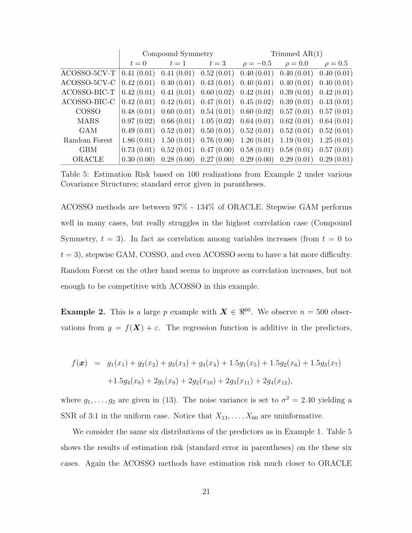
We consider the same six distributions of the predictors as in Example 1. Table 5

shows the results of estimation risk (standard error in parentheses) on the these six

cases. Again the ACOSSO methods have estimation risk much closer to ORACLE

21

n = 100 n = 250 n = 500ACOSSO-5CV-T 0.139 (0.017) 0.055 (0.001) 0.034 (0.001)ACOSSO-5CV-C 0.120 (0.011) 0.055 (0.001) 0.036 (0.001)ACOSSO-BIC-T 0.200 (0.027) 0.054 (0.001) 0.034 (0.001)ACOSSO-BIC-C 0.138 (0.016) 0.050 (0.001) 0.034 (0.001)

COSSO 0.290 (0.016) 0.093 (0.002) 0.057 (0.001)MARS 0.245 (0.021) 0.149 (0.009) 0.110 (0.008)GAM 0.149 (0.005) 0.137 (0.001) 0.136 (0.001)

Random Forest 0.297 (0.006) 0.190 (0.002) 0.148 (0.001)GBM 0.126 (0.003) 0.084 (0.001) 0.065 (0.001)

ORACLE 0.071 (0.003) 0.042 (0.001) 0.029 (0.000)

Table 6: Estimation Risk based on 100 realizations from Example 3 with n = 100,250, and 500; standard error given in parantheses.

than the other methods. COSSO and GAM have very similar performance in this

example and generally have the best risk among the methods other than ACOSSO.

One notable exception is the extremely high correlation case (Compound Symmetry,

t = 3, where Corr(Xj, Xk) = .9 for j 6= k). Here the ACOSSO-BIC-T and ACOSSO-

5CV-T seem to struggle a bit as they have risk near or above the risk of COSSO and

GAM. GBM actually has the best risk in this particular case. However, the ACOSSO

variants are substantially better overall than any of the other methods.

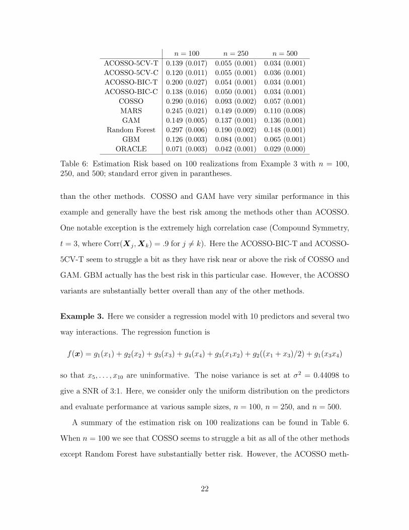
Example 3. Here we consider a regression model with 10 predictors and several two

way interactions. The regression function is

f(x) = g1(x1) + g2(x2) + g3(x3) + g4(x4) + g3(x1x2) + g2((x1 + x3)/2) + g1(x3x4)

so that x5, . . . , x10 are uninformative. The noise variance is set at σ2 = 0.44098 to

give a SNR of 3:1. Here, we consider only the uniform distribution on the predictors

and evaluate performance at various sample sizes, n = 100, n = 250, and n = 500.

A summary of the estimation risk on 100 realizations can be found in Table 6.

When n = 100 we see that COSSO seems to struggle a bit as all of the other methods

except Random Forest have substantially better risk. However, the ACOSSO meth-

22

n=100 n=250 n=500ACOSSO-BIC-T 3.84 25.10 89.02

COSSO 7.52 43.43 140.10MARS 9.15 11.23 13.64GAM 5.69 7.93 11.34

Random Forest 0.34 6.38 15.25GBM 4.15 9.14 17.01

Table 7: Average CPU time (in seconds) for each method to compute a model fit(including tuning parameter selection) for the various sample size simulations of Ex-ample 3.

ods have risk comparable or better than the other methods and less than half that of

COSSO. The estimation risk for all methods improves as the sample size increases.

However, stepwise GAM does not improve from n = 250 to n = 500 probably be-

cause of it’s inability to model the interactions in this example. Also notice that the

ACOSSO methods maintain close to 50% the risk of COSSO for all sample sizes. In

fact, for n = 500 the ACOSSO methods have risk nearly the same as that of the

ORACLE and roughly half that of the next best methods (COSSO and GBM).

Computation Time. Table 7 gives the computation times (in seconds) for the

various methods on the three sample size cases in Example 3. The times given are the

average over the 100 realizations and include the time required for tuning parameter

selection.

For larger sample sizes, ACOSSO and COSSO take significantly longer than the

other methods. COSSO takes longer that ACOSSO because of the 5CV tuning pa-

rameter selection used for COSSO as opposed to BIC tuning parameter selection used

in ACOSSO. If 5CV were used for ACOSSO, the computing time would be similar

to COSSO. It is important to point out that the other methods (besides ACOSSO

or COSSO) are computed via more polished R-packages that take advantage of the

speed of compiled languages such as C or Fortran. The computing time of ACOSSO

(and COSSO) could also be decreased substantially by introducing more efficient

23

approximations and by taking advantage of a compiled language.

7 Application to Real Data

In this section we apply the ACOSSO to three real datasets. We only report the

results of the two ACOSSO-BIC methods since they performed much better over-

all than the ACOSSO-5CV methods in our simulations. The first two data sets

are the popular Ozone data and the Tecator data which were also used by Lin &

Zhang (2006). Both data sets are available from the datasets archive of StatLib at

http://lib.stat.cmu.edu/datasets/. The Ozone data was also used in Breiman

& Friedman (1995), Buja, Hastie & Tibshirani (1989), and Breiman (1995). This data

set contains the daily maximum one-hour-average ozone reading and 8 meteorological

variables recorded in the Los Angeles basin for 330 days of 1976.

The Tecator data was recorded on a Tecator Infratec Food and Feed Analyzer.

Each sample contains finely chopped pure meat with different moisture, fat and pro-

tein contents. The input vector consists of a 100 channel spectrum of absorbances.

The absorbance is − log10 of the transmittance measured by the spectrometer. We

fit an additive model to predict fat content using the first 23 principal components

of the inputs as predictors. This is opposed to using a two way interaction model

on the first 13 principal components as in the COSSO paper. Our reasoning is that

additive functions of the principal component scores are already allowing for inter-

actions among the original inputs. In any case this approach seemed to produce the

best prediction of the fat content for all of the methods. The total sample size is 215.

The third data set comes from a computer model for two phase fluid flow (Vaughn,

Bean, Helton, Lord, MacKinnon & Schreiber 2000). Uncertainty/sensitivity analy-

sis of this model was carried out as part of the 1996 compliance certification ap-

plication for the Waste Isolation Pilot Plant (WIPP) (Helton & Marietta, editors

24

Ozone Tecator WIPPACOSSO-BIC-T 15.07 (0.07) 0.66 (0.02) 1.04 (0.00)ACOSSO-BIC-C 14.81 (0.08) 0.67 (0.01) 1.05 (0.01)

COSSO 15.99 (0.06) 0.41 (0.01) 1.30 (0.01)MARS 14.24 (0.12) 1.91 (0.24) 1.12 (0.01)GAM 15.91 (0.12) 1.48 (0.09) 1.83 (0.01)

Random Forest 18.11 (0.07) 4.38 (0.06) 1.29 (0.01)GBM 10.69 (0.00) 1.21 (0.00) 0.97 (0.00)

Table 8: Estimated Prediction Risk for Real Data Examples; standard error given inparantheses. Risk for BRNREPTC10K for the WIPP data is in units of 100m6

2000). There were 31 uncertain variables that were inputs into the two-phase fluid

flow analysis; see Storlie & Helton (2008) for a full description. Here we consider

only a specific scenario which was part of the overall analysis. The variable BRN-

REPTC10K is used as the response. This variable corresponds to cumulative brine

flow in m3 into the waste repository at 10,000 years assuming there was a drilling

intrusion at 1000 years. The sample size is n = 300. This data set is available at

http://www.stat.unm.edu/~storlie/acosso/.

We apply each of the methods on these three data sets and estimate the prediction

risk, E[Y −f(X)]2, by ten-fold cross validation. We select the tuning parameter using

only data within the training set (i.e. a new value of the tuning parameter is selected

for each of the 10 training sets without using any data from the test sets). The

estimate obtained is then evaluated on the test set. We repeat this ten-fold cross

validation 50 times and average. The resulting prediction risk estimates along with

standard errors are displayed in Table 8. The two way interaction model is presented

for all of the methods (except GAM) on the Ozone and WIPP examples since it had

better prediction accuracy than the additive model. As mentioned, an additive model

was used for all methods on the Tecator example.

For the Ozone data set, the ACOSSO is comparable to MARS but better than

COSSO, GAM and Random Forest. GBM seems to be the best method for predic-

tion accuracy on this data set though. For the Tecator data, both the COSSO and

25

ACOSSO are much better than all of the other methods. However, COSSO is better

than ACOSSO here which shows that the adaptive weights aren’t always an advan-

tage. The reason that COSSO performs better in this case is likely due to the fact

that all of the important functional components seem to have norms with similar mag-

nitudes. Also, the average number of components selected into the model is around

20 out of the 23 components so this is not a very sparse model either. Hence using

all weights equal to 1 (the COSSO) should work quite well here. In cases like this,

using adaptive weights in the ACOSSO can detract from the COSSO fit by adding

more noise to the estimation process. In contrast, the WIPP data set has only about

8 informative input variables of the 31 inputs with varying amounts of smoothness

for the functional components. Hence the ACOSSO significantly outperforms the

COSSO and is comparable to GBM for prediction accuracy.

8 Conclusions & Further Work

In this article, we have developed the ACOSSO, a new regularization method for

simultaneous model fitting and variable selection in the context of nonparametric

regression. The relationship between the ACOSSO and the COSSO is analogous

to that between the adaptive LASSO and the LASSO. We have explored a special

case under which the ACOSSO has a nonparametric version of the oracle property,

which the COSSO does not appear to possess. This is the first result of this type

for a nonparametric regression estimator. In addition we have demonstrated that

the ACOSSO outperforms COSSO, MARS, and stepwise GAMs for variable selection

and prediction on all simulated examples and all but one of the real data examples.

The ACOSSO also has very competitive performance for prediction when compared

with other well known prediction methods Random Forest and GBM. R code to fit

ACOSSO models is available at http://www.stat.unm.edu/∼storlie/acosso/.

26

It remains to show that ACOSSO has the np-oracle property under more general

conditions such as random designs. It may also be possible to yet improve the perfor-

mance of the ACOSSO by using a different weighting scheme. The Tecator example

in Section 7, suggests that using a weight power, γ = 2 is not always ideal. Perhaps

it would be better to cross validate on a few different choices of γ so that it could

be chosen smaller in cases (such as the Tecator example) where the weights are not

as helpful. In addition, there are certainly a number of other ways to use the initial

estimate, f , in the creation of the penalty term. These are topics for further research.

A Proofs

A.1 Equivalent Form

Proof of Lemma 1. Denote the functional in (6) by A(f) and the functional in (9) by

B(θ, f). Since a + b ≥ 2√

ab for a, b ≥ 0, with equality if and only if a = b, we have

for each j = 1, . . . , q

λ0θ−1j w2−ϑ

j ‖P jf‖2F + λ1w

ϑj θj ≥ 2λ

1/20 λ

1/21 wj‖P jf‖F = λwj‖P jf‖F ,

for any θj ≥ 0 and any f ∈ F . Hence B(θ, f) ≥ A(f) with equality only when

θj = λ1/20 λ

−1/21 w1−ϑ

j ‖P j f‖F and the result follows.

A.2 Convergence Rate

The proof of Theorem 1 uses Lemma 2 below which is a generalization of Theorem

10.2 of van de Geer (2000). Consider the regression model yi = g0(xi)+εi, i = 1, . . . , n

where g0 is known to lie in a class of functions G, xi’s are given covariates in [0, 1]p, and

εi’s are independent and sub-Gaussian as in (8). Let In : G → [0,∞) be a pseudonorm

on G. Define gn = arg ming∈G 1/n∑n

i=1(yi − g(xi))2 + τ 2

nIn(g). Let H∞(δ,G) be the

27

δ-entropy of the function class G under the supremum norm ‖g‖∞ = supx |g(x)| (see

van de Geer 2000 page 17).

Lemma 2. Suppose there exists I∗ such that I∗(g) ≤ In(g) for all g ∈ G, n ≥ 1. Also

assume that there exists constants A > 0 and 0 < α < 2 such that

H∞

(δ,

{g − g0

I∗(g) + I∗(g0): g ∈ G, I∗(g) + I∗(g0) > 0

})≤ Aδ−α (A1)

for all δ > 0 and n ≥ 1. Then if I∗(g0) > 0 and τ−1n = Op

(n1/(2+α)

)I

(2−α)/(4+2α)n (g0),

we have ‖gn − g0‖ = Op(τn)I1/2n (g0). Moreover, if In(g0) = 0 for all n ≥ 1 then

‖gn − g0‖ = Op(n−1/(2−α))τ

−2α/(2−α)n .

Proof. This follows the same logic as the proof of Theorem 10.2 of van de Geer (2000),

so we have intentionally made the following argument somewhat terse. Notice that

‖gn − g0‖2n + τ 2

nIn(gn) ≤ 2(ε, gn − g0)n + τ 2nIn(g0). (A2)

Also, condition (A1) along with Lemma 8.4 in van de Geer (2000) guarantees that

supg∈G

|(ε, gn − g0)n|‖gn − g0‖1−α/2

n (I∗(g) + I∗(g0))α/2= Op(n

−1/2). (A3)

Case (i) Suppose that I∗(gn) > I∗(g0). Then by (A2) and (A3) we have

‖gn − g0‖2n + τ 2

nIn(gn) ≤ Op(n−1/2)‖gn − g0‖1−α/2

n Iα/2∗ (gn) + τ 2

nIn(g0)

≤ Op(n−1/2)‖gn − g0‖1−α/2

n Iα/2n (gn) + τ 2

nIn(g0).

The rest of the argument is identical to that on page 170 of van de Geer (2000).

Case (ii) Suppose that I∗(gn) ≤ I∗(g0) and I∗(g0) > 0. By (A2) and (A3) we have

‖gn − g0‖2n ≤ Op(n

−1/2)‖gn − g0‖1−α/2n Iα/2

∗ (g0) + τ 2nIn(g0)

≤ Op(n−1/2)‖gn − g0‖1−α/2

n Iα/2n (g0) + τ 2

nIn(g0).

The remainder of this case is identical to that on page 170 of van de Geer (2000).

Proof of Theorem 1. The conditions of Lemma 2 do not hold directly for the F and

In(f) =∑p

j=1 wj,n‖P jf‖F of Theorem 1. The following orthogonality argument used

28

in van de Geer (2000) and Lin & Zhang (2006) works to remedy this problem though.

For any f ∈ F we can write f(x) = b + g(x) = b + f1(x1) + · · · + fp(xp), such that∑ni=1 fj(xj,i) = 0, j = 1, . . . , p. Similarly write f(x) = b+g(x) and f0(x) = b0+g0(x).

Then∑n

i=1(g(xi)− g0(xi)) = 0, and we can write (6) as

(b0 − b)2 +2

n(b0 − b)

n∑i=1

εi +1

n

n∑i=1

(g0(xi)− g(xi))2 + λn

p∑j=1

wj,n‖P jg‖F .

Therefore b must minimize (b0 − b)2 + 2/n(b0 − b)∑n

i=1 εi so that b = b0 + 1/n∑

i εi.

Hence (b− b0)2 = Op(n

−1). On the other hand, g must minimize

1

n

n∑i=1

(g0(xi)− g(xi))2 + λn

p∑j=1

wj,n‖P jg‖F (A4)

over all g ∈ G where

G = {g ∈ F : g(x) = f1(x1) + · · ·+ fp(xp),n∑

i=1

fj(xj,i) = 0, j = 1, . . . , p}. (A5)

Now rewrite (A4) as

1

n

n∑i=1

(g0(xi)− g(xi))2 + λn

p∑j=1

wj,n‖P jg‖F , (A6)

where λn = λnw∗,n, w∗,n = min{w1,n, . . . , wp,n}, and wj,n = wj,n/w∗,n.

The problem is now reduced to showing that the conditions of Lemma 2 hold for

τ 2n = λn and In(g) =

∑pj=1 wj,n‖P jg‖F . However, notice that min{w1,n, . . . , wp,n} = 1

for all n. This implies that In(g) ≥ I∗(g) =∑p

j=1 ‖P jg‖F for all g ∈ G and n ≥ 1.

Also notice that the entropy bound in (A1) holds whenever

H∞(δ, {g ∈ G : I∗(g) ≤ 1}) ≤ Aδ−α, (A7)

since I∗(g − g0) ≤ I∗(g) + I∗(g0) so that the set in brackets in (A7) contains that in

(A1). And (A7) holds by Lemma 4 in the COSSO paper with α = 1/2. We complete

the proof by treating the cases U c not empty and U c empty separately.

Case (i) Suppose that P jf 6= 0 for some j. Then I∗(g0) > 0. Also, w−1∗,n = Op(1) and

29

wj,n = Op(1) for j ∈ U c by assumption. This implies that wj,n = Op(1), for j ∈ U c so

that In(g0) = Op(1). Also λ−1n = Op(1)λ−1

n = Op(n4/5). The result now follows from

Lemma 2.

Case (ii) Suppose now that P jf = 0 for all j. Then In(g0) = 0 for all n and the result

follows from Lemma 2.

Proof of Corollary 1. For the traditional smoothing spline with λ0 ∼ n−4/5 it is known

(Lin 2000) that ‖P j f − P jf0‖L2 = Op(n−2/5). This implies |‖P j f‖L2 − ‖P jf0‖L2| ≤

Op(n−2/5). Hence w−1

j,n = Op(1) for j = 1, . . . , p and wj,n = Op(1) for j ∈ U c, which

also implies w∗,n = Op(1). The conditions of Theorem 1 are now satisfied and we

have ‖f − fn‖ = Op(n−2/5) if P jf 6= 0 for some j. On the other hand, also notice

that w−1j,n = Op(n

−2γ/5) for j ∈ U . Hence w−1∗,n = Op(n

−2γ/5) whenever P jf = 0 for all

j so that n−2/3λ−1/3n w

−1/3∗,n = Op(n

−1/2) for γ > 3/4 and the result follows.

A.3 Oracle Property

Proof of Theorem 2. Define Σ = {K(x1,i, x1,j)}mi,j=1, the m×m marginal Gram ma-

trix corresponding to the reproducing kernel for S2per. Also let Kj stand for the

n × n Gram matrix corresponding to the reproducing kernel for S2per on variable xj,

j = 1, . . . , p. Let 1m be a vector of m ones. Assuming the observations are permuted

appropriately, we can write

K1 = Σ⊗ (1m1′m)⊗ · · · ⊗ (1m1′m)

K2 = (1m1′m)⊗Σ⊗ · · · ⊗ (1m1′m)

...

Kp = (1m1′m)⊗ · · · ⊗ (1m1′m)⊗Σ,

where ⊗ here stands for the Kronecker product between two matrices.

30

Straightforward calculation shows that Σ1m = 1/(720m3)1m. So write the eigen-

vectors of Σ as {υ1 = 1m, υ2, . . . ,υm} and let Υ be the m × m matrix with these

eigenvectors as its columns. The corresponding eigenvalues are {mφ1, mφ2, . . . ,mφm},

where φ1 = 1/(720m4) and φ2 ≥ φ3 ≥ · · · ≥ φm. It is known (Uteras 1983) that

φi ∼ i−4 for i ≥ 2. Notice {υ1, υ2, . . . ,υm} are also the eigenvectors of (1m1′m) with

eigenvalues {m, 0, . . . , 0}. Write O = Υ⊗Υ⊗ · · · ⊗Υ and let ξi be the ith column

of O, i = 1, . . . , n. It is easy to verify that {ξ1, . . . , ξn} form an eigensystem for each

of K1, . . . ,Kp.

Let {ζ1,j, . . . , ζn,j} be the collection of vectors {ξ1, . . . , ξn} sorted so that those

corresponding to nonzero eigenvalues for Kj are listed first. Specifically, let

ζi,1 = υi ⊗ 1m ⊗ · · · ⊗ 1m,

ζi,2 = 1m ⊗ υi ⊗ · · · ⊗ 1m,

... (A8)

ζi,p = 1m ⊗ 1m ⊗ · · · ⊗ υi,

for i = 1, . . . ,m. Notice that each ζi,j, i = 1, . . . ,m, j = 1, . . . , p corresponds to

a distinct ξk, for some k ∈ {1, . . . , n}. So let the first m elements of the collection

{ζ1,j, . . . , ζm,j, ζm+1,j, . . . , ζn,j} be given by (A8) and the remaining n −m be given

by the remaining ξi in any order. The corresponding eigenvalues are then

ηi,j =

{nφi for i = 1, . . . ,m

0 for i = m + 1, . . . , n.

It is clear that {ξ1, . . . , ξn} is also an orthonormal basis in <n with respect to the

inner product〈u, v〉n = 1/n

∑i

uivi. (A9)

Let f = (f(x1), . . . , f(xn))′. Denote a = (1/n)O′f and z = (1/n)O′y. That is,

zi = 〈y, ξi〉n, ai = 〈f , ξi〉n, δi = 〈ε, ξi〉n and we have that zi = ai + δi. With some

abuse of notation, also let

31

zi,j =⟨y, ζi,j

⟩n, ai,j =

⟨f , ζi,j

⟩n, δi,j =

⟨ε, ζi,j

⟩n.

Now, using ϑ = 2 in (9), the ACOSSO estimate is the minimizer of

1

n(y −Kθc− b1n)′(y −Kθc− b1n) + c′Kθc + λ1

p∑j=1

w2jθj, (A10)

where Kθ =∑p

j=1 θjKj. Let s = O′c and Dj = (1/n2)O′KjO is a diagonal matrix

with diagonal elements φi. Then (A10) is equivalent to

(z −Dθs− (b, 0, ..., 0)′)′(z −Dθs− (b, 0, ..., 0)′) + s′Dθs + λ1

p∑j=1

w2jθj, (A11)

where Dθ =∑p

j=1 θjDj. Straightforward calculation shows that this minimization

problem is equivalent to

`(s, θ) =m∑

i=1

p∑j=1

(zij − φiθjsij)2 +

m∑i=1

p∑j=1

φiθjs2ij + λ1

p∑j=1

w2jθj, (A12)

where sij = ζ ′ijc, i = 1, . . . ,m, j = 1, . . . , p are distinct elements of s.

Now, we first condition on θ and minimize over s. Given θ, `(s, θ) is a convex

function of s and is minimized at s(θ) = {sij(θj)}m pi=1 j=1, where sij(θj) = zij(1−φiθj).

Inserting s(θ) into (A12) gives

`(s(θ), θ) =m∑

i=1

p∑j=1

z2ij

(1 + φiθj)2+

m∑i=1

p∑j=1

φiθjz2ij

(1 + φiθj)2+ λ1

p∑j=1

w2jθj

=m∑

i=1

p∑j=1

z2ij

1 + φiθj

+ λ1

p∑j=1

w2jθj. (A13)

Notice that `(s(θ), θ) is continuous in θj,

∂2`(s(θ), θ)

∂θ2j

= 2m∑

i=1

z2ijφ

2i

(1 + φiθj)3> 0 for each j (A14)

and ∂2`(s(θ), θ)/∂θj∂θk = 0 for j 6= k. Therefore `(s, θ) is convex and has a unique

minimum, θ.

Clearly, P j f ≡ 0 if and only if θj = 0. So it suffices to consider θj. As such, since

we must have that θj ≥ 0, the minimizer, θj = 0 if and only if

32

∂

∂θj

` (s(θ), θ)

∣∣∣∣θj=0

≥ 0,

which is equivalent to

T = n

m∑i=1

φiz2ij ≤ nw2

j,nλ1,n. (A15)

If we assume that P jf = 0, then we have zij = δij. In the following, we will obtain

bounds for E(T ) and Var(T ) to demonstrate that T is bounded in probability when

P jf = 0. To this end, we first obtain bounds for E(δ2ij) and Var(δ2

ij). Recall that

δij = (1/n)ζ ′ijε and that the individual elements of ε are independent with E(ε) = 0.

For notational convenience, let ξ = ζij which is some column of the O matrix. Also,

recall that the vector ξ is orthonormal with respect to the inner product in (A9).

Now,

E(δ2ij) =

1

n2E[(ξ′ε)2]

=1

n2E

(n∑

a=1

n∑b=1

ξaξbεaεb

)

=1

n2

n∑a=1

ξ2aE(ε2

a)

≤ 1

n2

n∑a=1

ξ2aM1

=M1

n(A16)

where M1 = maxa E(ε2a) which is bounded because of the sub-Gaussian condition (8).

The variance of δ2ij is

Var(δ2ij) = Var

(n∑

a=1

n∑b=1

ξaξbεaεb

)

=n∑

a=1

n∑b=1

n∑c=1

n∑d=1

ξaξbξcξdCov(εaεb , εcεd). (A17)

But εa’s are independent, so Cov(εaεb , εcεd) 6= 0 only in the three mutually exclusive

cases (i) a = b = c = d, (ii) a = c and b = d with a 6= b, or (iii) a = d and b = c with

33

a 6= b. Thus, (A17) becomes,

Var(δ2ij) =

1

n4

[n∑

a=1

ξ4aCov(ε2

a , ε2a) + 2

n∑a=1

n∑b6=a

ξ2aξ

2b Cov(εaεb , εaεb)

]

≤ 2

n4

n∑a=1

n∑b=1

ξ2aξ

2b Var(εaεb)

≤ 2M2

n4

(n∑

a=1

ξ2a

)2

=2M2

n2(A18)

where M2 = maxa,b{Var(εaεb)} which is bounded because of the sub-Gaussian con-

dition in (8). Notice that the derivations of the bounds in (A16) and (A18) do not

depend on i or j (i.e. they do not depend on which column of O that ξ comes from).

Thus, the bounds in (A16) and (A18) are uniform for all i.

Using (A16) we can write E(T ) as

E(T ) = nm∑

i=1

φiE[δ2ij] ≤ M1

m∑i=1

φi ∼ M1. (A19)

Further, we can use (A18) to write Var(T ) as

Var(T ) = n2Var

(m∑

i=1

φiδij

)

= n2

m∑k=1

m∑l=1

φkφlCov(δ2k,j, δ

2l,j)

≤ 2M2

m∑k=1

m∑l=1

φkφl

= 2M2

(m∑

k=1

φk

)2

∼ 2M2. (A20)

Finally, as n increases, (A19) and (A20) guarantee that the left-hand side of

34

(A15) is bounded in probability when P jf = 0. Assuming that nw2j,nλ

2n

p→ ∞ or

equivalently that nw2j,nλ1,n

p→ ∞ by Lemma 1, the right-hand side of (A15) increases

to ∞ in probability. Therefore, if P jf = 0 then θj = 0 with probability tending to

one. If on the other hand nw2j,nλ

2n = Op(1), then the probability that T > nw2

j,nλ1,n

converges to a positive constant. Hence the probability that θj > 0 converges to a

positive constant.

Proof of Corollary 2. It is straightforward to to show that Theorem 1 still holds with

S2per in place of S2. Also recall from the proof of Corollary 1 that these weights

satisfy the conditions of Theorem 1. Also, since w−1j,n = Op(n

−2γ/5) for j ∈ U we have

nw2j,nλ

2n

p→ ∞ for j ∈ U whenever γ > 3/4. The conditions of Theorem 2 are now

satisfied. Lastly, in light of Theorem 1, we also know that if P jf 6= 0, the probability

that P j f 6= 0 also tends to one as the sample size increases due to the consistency.

Corollary 2 follows.

References

Berlinet, A. & Thomas-Agnan, C. (2004), Reproducing Kernel Hilbert Spaces in Prob-ability and Statistics, Norwell, MA: Kluwer Academic Publishers.

Breiman, L. (1995), ‘Better subset selection using the nonnegative garrote’, Techno-metrics 37, 373–384.

Breiman, L. (2001), ‘Random forests’, Machine Learning 45, 5–32.

Breiman, L. & Friedman, J. (1995), ‘Estimating optimal transformations for multi-ple regression and correlation’, Journal of the American Statistical Association80, 580–598.

Buja, A., Hastie, T. & Tibshirani, R. (1989), ‘Linear smoothers and additive models(with discussion)’, Annals of Statistics 17, 453–555.

Cleveland, W. (1979), ‘Robust locally weighted fitting and smoothing scatterplots’,Journal of the American Statistical Association 74, 829–836.

Craven, P. & Wahba, G. (1979), ‘Smoothing noisy data with spline functions: es-timating the correct degree of smoothing by the method of generalized cross-validation’, Numerical Mathematics 31, 377–403.

35

Efromovich, S. & Samarov, A. (2000), ‘Adaptive estimation of the integral of squaredregression derivatives’, Scandinavian Journal of Statistics 27, 335–351.

Fan, J. & Li, R. (2001), ‘Variable selection via nonconcave penalized likelihood andits oracle properties’, Journal of the American Statistical Association 96, 1348–1360.

Friedman, J. (1991), ‘Multivariate adaptive regression splines (with discussion)’, An-nals of Statistics 19, 1–141.

Friedman, J. (2001), ‘Greedy function approximation: A gradient boosting machine’,Annals of Statistics 29, 1189–1232.

Goldfarb, D. & Idnani, A. (1982), Dual and Primal-Dual Methods for SolvingStrictly Convex Quadratic Programs. In Numerical Analysis J.P. Hennart (ed.),Springer-Verlag, Berlin.

Gu, C. (2002), Smoothing Spline ANOVA Models, Springer-Verlag, New York, NY.

Hastie, T. & Tibshirani, R. (1990), Generalized Additive Models, Chapman &Hall/CRC.

Helton, J. & Marietta, editors, M. (2000), ‘Special issue: The 1996 performance as-sessment for the Waste Isolation Pilot Plant’, Reliability Engineering and SystemSafety 69(1-3), 1–451.

Knight, K. & Fu, W. (2000), ‘Asymptotics for lasso-type estimators’, Annals of Statis-tics 28, 1356–1378.

Lin, Y. (2000), ‘Tensor product space anova models’, Annals of Statistics 28, 734–755.

Lin, Y. & Zhang, H. (2006), ‘Component selection and smoothing in smoothing splineanalysis of variance models’, Annals of Statistics 34, 2272–2297.

Nadaraya, E. (1964), ‘On estimating regression’, Theory of Probability and its Appli-cations 9, 141–142.

Schimek, M., ed. (2000), Smoothing and Regression: Approaches, Computation, andApplication, John Wiley & Sons, Inc., New York, NY.

Schwarz, G. (1978), ‘Estimating the dimension of a model’, Annals of Statistics6, 461–464.

Stone, C., Buja, A. & Hastie, T. (1994), ‘The use of polynomial splines andtheir tensor-products in multivariate function estimation’, Annals of Statistics22, 118–184.

36

Stone, C., Hansen, M., Kooperberg, C. & Truong, Y. (1997), ‘1994 wald memoriallectures - polynomial splines and their tensor products in extended linear mod-eling’, Annals of Statistics 25, 1371–1425.

Storlie, C. & Helton, J. (2008), ‘Multiple predictor smoothing methods for sensitivityanalysis: Example results’, Reliability Engineering and System Safety 93, 55–77.

Tibshirani, R. (1996), ‘Regression shrinkage and selection via the lasso’, Journal ofthe Royal Statistical Society: Series B 58, 267–288.

Uteras, F. (1983), ‘Natural spline functions: Their associated eigenvalue problem’,Numerische Mathematik 42, 107–117.

van de Geer, S. (2000), Empirical Processes in M-Estimation, Cambridge UniversityPress.

Vaughn, P., Bean, J., Helton, J., Lord, M., MacKinnon, R. & Schreiber, J. (2000),‘Representation of two-phase flow in the vicinity of the repository in the 1996performance assessment for the Waste Isolation Pilot Plant’, Reliability Engi-neering and System Safety 69(1-3), 205–226.

Wahba, G. (1990), Spline Models for Observational Data, CBMS-NSF Regional Con-ference Series in Applied Mathematics.

Wahba, G., Wang, Y., Gu, C., Klein, R. & Klein, B. (1995), ‘Smoothing spline anovafor exponential families, with application to the WESDR’, Annals of Statistics23, 1865–1895.

Zou, H. (2006), ‘The adaptive lasso and its oracle properties’, Journal of the AmericanStatistical Association 101(476), 1418–1429.

Zou, H., Hastie, T. & Tibshirani, R. (2007), ‘On the ”degrees of freedom” of thelasso’, Annals of Statistics 35(5), 2173–2192.

37