Suppplementary Information: “Mechanical oscillation and cooling actuated

by the optical gradient force”

Qiang Lin, Jessie Rosenberg, Xiaoshun Jiang, Kerry Vahala, Oskar Painter∗

Thomas J. Watson, Sr., Laboratory of Applied Physics,

California Institute of Technology, Pasadena, CA 91125

(Dated: May 4, 2009)

Abstract

We present in this supporting material to our manuscript entitled, “Mechanical oscillation and cooling

actuated by optical gradient forces,” the detailed analysis related to estimates of the optical gradient force

and effective motion mass, modeling of the optical cavity transmission and its power spectrum, simulations

of optomechanical oscillation, and the effective cooling of the micro-mechanical system.

∗Electronic address: opainter@caltech.edu; URL: http://copilot.caltech.edu

1

I. OPTICAL GRADIENT FORCE IN A DOUBLE-DISK NOMS

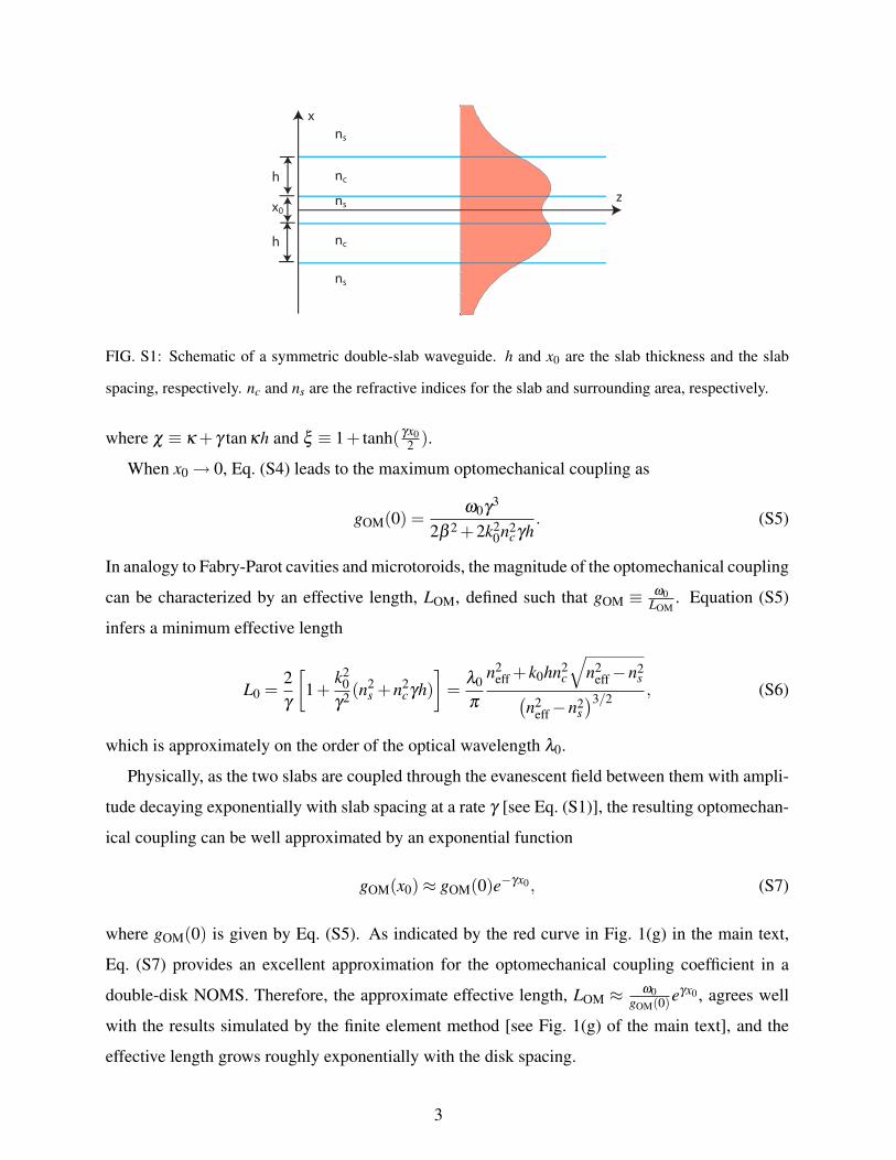
As the mode confinement in a double-disk NOMS is primarily provided by the transverse

boundaries formed by the two disks, the double-disk structure can be well approximated by a

symmetric double-slab waveguide shown in Fig. S1. For the bonding mode polarized along the ey

direction, the tangential component of the electric field is given by:

Ey =

Ae−γx, x > h+ x0/2

Bcosκx+C sinκx, x0/2 < x < h+ x0/2

Dcoshγx, −x0/2 < x < x0/2

Bcosκx−C sinκx, −x0/2 > x >−h− x0/2

Aeγx, x <−h− x0/2

(S1)

where κ is the transverse component of the propagation constant inside the slabs and γ is the field

decay constant in the surrounding area. They are given by the following expressions:

κ2 = k2

0n2c−β

2, γ2 = β

2− k20n2

s , (S2)

where k0 = ω0/c is the propagation constant in vacuum and β = k0neff is the longitudinal com-

ponent of the propagation constant of the bonding mode. neff is the effective refractive index for

the guided mode. Accordingly, the tangential component of the magnetic field can be obtained

through Hz = −iµω0

∂Ey∂x . The continuity of Ey and Hz across the boundaries requires κ and γ to

satisfy the following equation:

κγ [1+ tanh(γx0/2)] =[κ

2− γ2 tanh(γx0/2)

]tanκh, (S3)

which reduces to tanκh = γ/κ when x0→ 0, as expected.

The circular geometry of the double disk forms the whispering-gallery mode, in which the

resonance condition requires the longitudinal component of the propagation constant, β , to be

fixed as 2πRβ = 2mπ , where R is the mode radius and m is an integer. Thus, any variation on

the disk spacing x0 transfers to a variation on the resonance frequency ω0 through Eqs. (S2) and

(S3), indicating that ω0 becomes a function of x0. By using these two equations, we find that the

optomechanical coupling coefficient, gOM = dω0dx0

, is given by the general form

gOM(x0) =cχγ2

k0sech2 ( γx0

2

)4(n2

c−n2s ) tanκh+n2

s x0χsech2 ( γx02

)+2ξ

[(n2

cγhcsc2 κh+2n2s ) tanκh+ n2

s κ

γ− n2

cγ

κ

] ,(S4)

2

h

h

x0z

x

nc

ns

ns

ns

nc

FIG. S1: Schematic of a symmetric double-slab waveguide. h and x0 are the slab thickness and the slab

spacing, respectively. nc and ns are the refractive indices for the slab and surrounding area, respectively.

where χ ≡ κ + γ tanκh and ξ ≡ 1+ tanh( γx02 ).

When x0→ 0, Eq. (S4) leads to the maximum optomechanical coupling as

gOM(0) =ω0γ3

2β 2 +2k20n2

cγh. (S5)

In analogy to Fabry-Parot cavities and microtoroids, the magnitude of the optomechanical coupling

can be characterized by an effective length, LOM, defined such that gOM ≡ ω0LOM

. Equation (S5)

infers a minimum effective length

L0 =2γ

[1+

k20

γ2 (n2s +n2

cγh)]

=λ0

π

n2eff + k0hn2

c

√n2

eff−n2s(

n2eff−n2

s)3/2 , (S6)

which is approximately on the order of the optical wavelength λ0.

Physically, as the two slabs are coupled through the evanescent field between them with ampli-

tude decaying exponentially with slab spacing at a rate γ [see Eq. (S1)], the resulting optomechan-

ical coupling can be well approximated by an exponential function

gOM(x0)≈ gOM(0)e−γx0, (S7)

where gOM(0) is given by Eq. (S5). As indicated by the red curve in Fig. 1(g) in the main text,

Eq. (S7) provides an excellent approximation for the optomechanical coupling coefficient in a

double-disk NOMS. Therefore, the approximate effective length, LOM ≈ ω0gOM(0)eγx0 , agrees well

with the results simulated by the finite element method [see Fig. 1(g) of the main text], and the

effective length grows roughly exponentially with the disk spacing.

3

II. EFFECTIVE MOTIONAL MASS FOR THE FLAPPING MODE

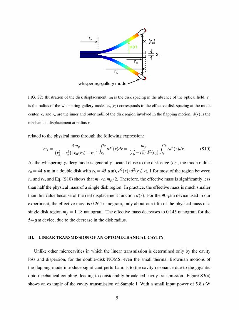
With a clamped inner edge and a free outer edge, the mechanical displacement of a double

disk exhibiting a flapping mode is generally a function of radius (Fig. S2). What matters the op-

tomechanical effect, however, is the disk spacing at the place where the whispering-gallery mode

is located, as that determines the magnitude of the splitting between the bonding and antibond-

ing cavity modes. As the mechanical displacement actuated by the gradient force is generally

small compared with the original disk spacing x0, we can assume it is uniform in the region of

the whispering-gallery mode and define the effective disk spacing xm(r0) at the mode center,

where r0 is the radius of the whispering-gallery mode. The effective mechanical displacement

is then given by xeff = xm(r0)− x0, corresponding to an effective mechanical potential energy of

Ep = mxΩ2mx2

eff/2, where mx is the corresponding effective motional mass and Ωm is the resonance

frequency of the flapping mode. Note that xeff is twice as the real displacement at the mode center

for a single disk, xeff = 2d(r0). Ep reaches its maximum value when the double disk is at rest at its

maximum displacement, at which point all of the mechanical energy is stored in the strain energy

Us. Therefore, Ep = Us and the effective motional mass is given by

mx =2Us

Ω2m[xm(r0)− x0]2

=Us

2Ω2md2(r0)

, (S8)

where both Us and d(r0) can be obtained from the mechanical simulations by the finite element

method.

The relationship between the effective mass and the physical mass of the double-disk NOMS

can be found by examining the mechanical potential energy. With a mechanical displacement d(r)

for each single disk [Fig. S2], we can find the total mechanical potential energy by integrating over

the disk regions involved in the flapping motion:

Ep =∫ rb

ra

Ω2md2(r)ζ 2πrhdr, (S9)

where ζ is the material density, h is the thickness for a single disk, ra and rb are the inner and

outer radii of the disk region involved in the flapping motion (see Fig. S2). Note that Ep is the

total potential energy for the two disks, which is simply two times that of single one because of

the symmetry between the two disks. As the physical mass of a single disk region involving in the

flapping motion is given by mp = πζ h(r2b− r2

a), using Eq. (S9), we find that the effective mass is

4

x0

xm(r0)

r0

whispering-gallery mode

d(r)

ra

rb

FIG. S2: Illustration of the disk displacement. x0 is the disk spacing in the absence of the optical field. r0

is the radius of the whispering-gallery mode. xm(r0) corresponds to the effective disk spacing at the mode

center. ra and rb are the inner and outer radii of the disk region involved in the flapping motion. d(r) is the

mechanical displacement at radius r.

related to the physical mass through the following expression:

mx =4mp(

r2b− r2

a)[xm(r0)− x0]

2

∫ rb

ra

rd2(r)dr =mp(

r2b− r2

a)

d2(r0)

∫ rb

ra

rd2(r)dr. (S10)

As the whispering-gallery mode is generally located close to the disk edge (i.e., the mode radius

r0 = 44 µm in a double disk with rb = 45 µm), d2(r)/d2(r0) 1 for most of the region between

ra and rb, and Eq. (S10) shows that mx mp/2. Therefore, the effective mass is significantly less

than half the physical mass of a single disk region. In practice, the effective mass is much smaller

than this value because of the real displacement function d(r). For the 90-µm device used in our

experiment, the effective mass is 0.264 nanogram, only about one fifth of the physical mass of a

single disk region mp = 1.18 nanogram. The effective mass decreases to 0.145 nanogram for the

54-µm device, due to the decrease in the disk radius.

III. LINEAR TRANSMISSION OF AN OPTOMECHANICAL CAVITY

Unlike other microcavities in which the linear transmission is determined only by the cavity

loss and dispersion, for the double-disk NOMS, even the small thermal Brownian motions of

the flapping mode introduce significant perturbations to the cavity resonance due to the gigantic

opto-mechanical coupling, leading to considerably broadened cavity transmission. Figure S3(a)

shows an example of the cavity transmission of Sample I. With a small input power of 5.8 µW

5

1516 1520 1524 1528 15320

0.2

0.4

0.6

0.8

1

Wavelength (nm)

No

rma

lize

d T

ran

smis

sio

n

(b)

0.94

0.96

0.98

1

−30 −20 −10 0 10 20 30[λ−1518.57nm] (pm)

Qi = 1.75 106

−10 −5 0 5 10

0.4

0.6

0.8

1

Wavelength Detuning (pm)

No

rma

lize

d T

ran

smis

sio

n

(a)

FIG. S3: (a) The cavity transmission of Sample I in a nitrogen environment, when the laser is scanned across

the cavity resonance at 1518.57 nm with an input power of 5.8 µW. The blue curve is the instantaneous

signal collected by the high-speed detector and the red curve is the average signal collected by the slow

reference detector 2. The slight asymmetry in the transmission spectrum is due to the static component

of mechanical actuation when the laser is scanned from blue to red. The dashed line indicates the laser

frequency detuning used to record the power spectral density shown in the top panel of Fig. 3(b) in the main

text. (b) Linear scan of the averaged cavity transmission of Sample I at an input power of 2.9 µW. The

inset shows a detailed scan for the bonding mode at 1518.57nm, with the experimental data in blue and the

theoretical fitting in red.

well below the oscillation threshold, the cavity transmission exhibits intense fluctuations when the

laser frequency is scanned across the cavity resonance. As a result, the averaged spectrum of the

cavity transmission (red curve) is significantly broader than the real cavity resonance. A correct

description of the cavity transmission requires an appropriate inclusion of the optomechanical

effect, which is developed in the following.

When the optical power is well below the oscillation threshold and the flapping mode of the

double disk is dominantly driven by thermal fluctuations, the mechanical motion can be described

by the following equation:d2xdt2 +Γm

dxdt

+Ω2mx =

FT (t)mx

, (S11)

where Ωm, Γm, and mx are the resonance frequency, damping constant, and effective mass of the

flapping mode, respectively. FT is the Langevin force driving the mechanical Brownian motion, a

Markovin process with the following correlation function:

〈FT (t)FT (t + τ)〉= 2mxΓmkBT δ (τ), (S12)

6

where T is the temperature and kB is Boltzmann’s constant. It can be shown easily from Eqs. (S11)

and (S12) that the Brownian motion of the flapping mode is also a Markovin process with a spectral

correlation given by 〈x(Ω1)x∗(Ω2)〉= 2πSx(Ω1)δ (Ω1−Ω2), where x(Ω) is the Fourier transform

of the mechanical displacement x(t) defined as x(Ω) =∫+∞

−∞x(t)eiΩtdt, and Sx(Ω) is the spectral

intensity for the thermal mechanical displacement with the following form:

Sx(Ω) =2ΓmkBT/mx

(Ω2m−Ω2)2 +(ΩΓm)2 . (S13)

The time correlation of the mechanical displacement is thus given by

〈x(t)x(t + τ)〉= 12π

∫ +∞

−∞

Sx(Ω)e−iΩτdτ ≡ 〈x2〉ρ(τ)≈ 〈x2〉e−Γm|τ|/2 cosΩmτ, (S14)

where 〈x2〉= kBT/(mxΩ2m) is the variance of the thermal mechanical displacement and ρ(τ) is the

normalized autocorrelation function for the mechanical displacement.

To be general, we consider a doublet resonance in which two optical fields, one forward and the

other backward propagating, circulate inside the microcavity and couple via Rayleigh scattering

from the surface roughness. The optical fields inside the cavity satisfy the following equations:

da f

dt= (i∆0−κ/2− igOMx)a f + iηab + i

√κeAin, (S15)

dab

dt= (i∆0−κ/2− igOMx)ab + iηa f , (S16)

where a f and ab are the forward and backward whispering-gallery modes (WGMs), normalized

such that U j = |a j|2 ( j = f ,b) represents the mode energy. Ain is the input optical wave, normal-

ized such that Pin = |Ain|2 represents the input power. κ is the photon decay rate for the loaded

cavity, and κe is the photon escape rate associated with the external coupling. ∆0 = ω −ω0 is

the frequency detuning from the input wave to the cavity resonance and η is the mode coupling

coefficient. In the case of a continuous-wave input, Eqs. (S15) and (S16) provide a formal solution

of the forward WGM:

a f (t) = i√

κeAin

∫ +∞

0cos(ητ) f (τ)e−igOM

∫τ

0 x(t−τ ′)dτ ′dτ, (S17)

where f (τ) ≡ e(i∆0−κ/2)τ represents the cavity response. Using Eq. (S14), we find that the statis-

tically averaged intracavity field is given as:

〈a f (t)〉= i√

κeAin

∫ +∞

0cos(ητ) f (τ)e−

ε

2 h(τ)dτ, (S18)

7

where ε ≡ g2OM〈x2〉 and h(τ) is defined as

h(τ)≡∫∫

τ

0ρ(τ1− τ2)dτ1dτ2. (S19)

Similarly, we can find the averaged energy for the forward WGM as:

〈U f (t)〉 = κePin

∫∫ +∞

0f (τ1) f ∗(τ2)cos(ητ1)cos(ητ2)e−

ε

2 h(|τ1−τ2|)dτ1dτ2

=κePin

2κ

κ− iηκ−2iη

∫ +∞

0e−

ε

2 h(τ) [ fc(τ)+ f ∗s (τ)]dτ + c.c., (S20)

where f j(τ) ≡ e(i∆ j−κ/2)τ ( j = c,s), with ∆c = ∆0 + η and ∆s = ∆0−η . c.c. denotes complex

conjugate.

As the transmitted power from the double disk is given by

PT (t) = Pin +κeU f (t)+ i√

κe[A∗ina f (t)−Aina∗f (t)

], (S21)

the averaged cavity transmission, 〈T 〉 ≡ 〈PT 〉/Pin, thus takes the form

〈T 〉= 1− κeκi

2κ

[1− iηκe

κi(κ−2iη)

]∫ +∞

0e−

ε

2 h(τ) [ fc(τ)+ f ∗s (τ)]dτ + c.c.

. (S22)

In the case of a singlet resonance, η = 0 and Eq. (S22) reduces to the simple form expression

〈T 〉= 1− κeκi

κ

∫ +∞

0e−

ε

2 h(τ) [ f (τ)+ f ∗(τ)]dτ. (S23)

In the absence of opto-mechanical coupling, gOM = 0 and Eq. (S23) reduces to the conventional

form of

T = 1− κeκi

∆20 +(κ/2)2 , (S24)

as expected.

Using the theory developed above and fitting the experimental averaged cavity transmission

spectrum, we obtain the optical Q factor of the resonance, as shown in Fig. S3(b) for Sample I.

The same approach is used to describe the cavity transmission of Sample II, given in Fig. 3(a) of

the main text.

IV. POWER SPECTRAL DENSITY OF THE CAVITY TRANSMISSION

Here we provide the derivations of the power spectral density of the cavity transmission in the

presence of mechanical Brownian motion. We present two theories, one for the linear-perturbation

regime when the optomechanical effect is small, the other a non-perturbation theory accurate for

arbitrarily strong optomechanical effect.

8

A. The linear-perturbation theory

If the induced optomechanical perturbations are small, Eq. (S17) can be approximated as

a f (t)≈ i√

κeAin

∫ +∞

0cos(ητ) f (τ)

[1− igOM

∫τ

0x(t− τ

′)dτ′]

dτ. (S25)

In this case, the transmitted optical field can be written as AT (t) = Ain + i√

κea f (t)≈ A0 +δA(t),

where A0 is the transmitted field in the absence of the optomechanical effect and δA is the induced

perturbation. They take the following forms:

A0 = Ain

[1−κe

∫ +∞

0cos(ητ) f (τ)dτ

]≡ AinA0, (S26)

δA(t) = igOMκeAin

∫ +∞

0dτ cos(ητ) f (τ)

∫τ

0x(t− τ

′)dτ′. (S27)

The transmitted power then becomes P(t) = |AT (t)|2 ≈ |A0|2 +A∗0δA(t)+A0δA∗(t). It is easy to

show that 〈δA(t)〉 = 0 and 〈PT (t)〉 = |A0|2. As a result, the power fluctuations, δP(t) ≡ PT (t)−

〈PT (t)〉, become

δP(t)≈ gOMPin

∫ +∞

0dτu(τ)

∫τ

0x(t− τ

′)dτ′, (S28)

where u(τ) ≡ iκe cos(ητ)[A∗0 f (τ)− A0 f ∗(τ)]. By using Eq. (S14), we find the autocorrelation

function for the power fluctuation to be

〈δP(t)δP(t + t0)〉 ≈ εP2in

∫∫ +∞

0dτ1dτ2u(τ1)u(τ2)ψ(t0,τ1,τ2), (S29)

where ψ(t0,τ1,τ2) is defined as

ψ(t0,τ1,τ2)≡∫

τ1

0dτ′1

∫τ2

0dτ′2ρ(t0 + τ

′1− τ

′2). (S30)

Taking the Fourier transform of Eq. (S29), we obtain the power spectral density SP(Ω) of the

cavity transmission to be

SP(Ω)≈ g2OMP2

inH(Ω)Sx(Ω), (S31)

where Sx(Ω) is the spectral intensity of the mechanical displacement given in Eq. (S13) and H(Ω)

is the cavity transfer function given by

H(Ω) =∣∣∣∣ 1Ω

∫ +∞

0u(τ)(eiΩτ −1)dτ

∣∣∣∣2 . (S32)

In the case of a singlet resonance, the cavity transfer function takes the form:

H(Ω) =κ2

e[∆2

0 +(κ/2)2]2 4∆2

0(κ2i +Ω2)

[(∆0 +Ω)2 +(κ/2)2] [(∆0−Ω)2 +(κ/2)2]. (S33)

9

In most cases, the photon decay rate inside the cavity is much larger than the mechanical damp-

ing rate, κ Γm. For a specific mechanical mode at the frequency Ωm, the cavity transfer function

can be well approximated by H(Ω) ≈ H(Ωm). In particular, in the sideband-unresolved regime,

the cavity transfer function is given by a simple form of

H =4κ2

e κ2i ∆2

0[∆2

0 +(κ/2)2]4 . (S34)

Therefore, Eq. (S31) shows clearly that, if the optomechanical effect is small, the power spectral

density of the cavity transmission is directly proportional to the spectral intensity of the mechanical

displacement.

B. The non-perturbation theory

The situation becomes quite complicated when the optomechanical effects are large. From

Eq. (S21), the autocorrelation function for the power fluctuation of the cavity transmission,

δP(t)≡ PT (t)−〈PT 〉, is given by

〈δP(t1)δP(t2)〉 = κ2e 〈U f 1U f 2〉−κe〈

(A∗ina f 1−Aina∗f 1

)(A∗ina f 2−Aina∗f 2

)〉

+ iκ3/2e[〈U f 1

(A∗ina f 2−Aina∗f 2

)〉+ 〈U f 2

(A∗ina f 1−Aina∗f 1

)〉]

−[κe〈U f 〉+ i

√κe(A∗in〈a f 〉−Ain〈a∗f 〉

)]2, (S35)

where U f j = U f (t j) and a f j = a f (t j) ( j = 1,2). Equation (S35) shows that the autocorrelation

function involves various correlations between the intracavity energy and field, all of which can

be found using Eqs. (S14) and (S17). For example, we can find the following correlation for the

intracavity field:

〈(A∗ina f 1−Aina∗f 1

)(A∗ina f 2−Aina∗f 2

)〉

=−κeP2in

∫∫ +∞

0dτ1dτ2C1C2e−

ε

2 (h1+h2)[

f1 f2e−εψ + f1 f ∗2 eεψ + c.c.], (S36)

where, in the integrand, C j = cos(ητ j), h j = h(τ j), f j = f (τ j) (with j = 1,2), and ψ = ψ(t2−

t1,τ1,τ2). h(τ) and ψ(t2− t1,τ1,τ2) are given by Eqs. (S19) and (S30), respectively.

Equations (S19) and (S30) show that h(τ) and ψ(t2− t1,τ1,τ2) vary with time on time scales

of 1/Ωm and 1/Γm. However, in the sideband-unresolved regime, κ Γm and κ Ωm. As the

cavity response function f (τ) decays exponentially with time at a rate of κ/2, the integrand in

10

Eq. (S36) becomes negligible when τ1 2/κ or τ2 2/κ . Therefore, ψ(t2− t1,τ1,τ2) can be

well approximated as

ψ(t2− t1,τ1,τ2) =1

2π〈x2〉

∫ +∞

−∞

Sx(Ω)Ω2 e−iΩ(t2−t1)

(e−iΩτ1−1

)(eiΩτ2−1

)dΩ

≈ τ1τ2

2π〈x2〉

∫ +∞

−∞

Sx(Ω)e−iΩ(t2−t1)dΩ = τ1τ2ρ(t2− t1). (S37)

Similarly, h(τ)≈ τ2, since h(τ) = ψ(0,τ,τ). Therefore, Eq. (S36) becomes

〈(A∗ina f 1−Aina∗f 1

)(A∗ina f 2−Aina∗f 2

)〉 ≈ −κeP2

inΦ(∆t,C1C2), (S38)

where ∆t = t2− t1 and Φ(∆t,C1C2) is defined as

Φ(∆t,C1C2)≡∫∫ +∞

0dτ1dτ2C1C2e−

ε

2(τ21 +τ2

2)[

f1 f2e−ετ1τ2ρ + f1 f ∗2 eετ1τ2ρ + c.c.], (S39)

with ρ = ρ(∆t). Following a similar approach, we can find the other correlation terms in Eq. (S35).

Using these terms in Eq. (S35), we find that the autocorrelation function of the power fluctuations

is given by

〈δP(t1)δP(t2)〉 ≈ κ2e P2

inΦ(∆t,σ1σ2)−[κe〈U f 〉+ i

√κe(A∗in〈a f 〉−Ain〈a∗f 〉

)]2, (S40)

where σ j = σ(τ j) ( j = 1,2) and σ(τ) is defined as

σ(τ)≡[

1− κe(κ2 +2η2)κ(κ2 +4η2)

]cos(ητ)+

ηκe

κ2 +4η2 sin(ητ). (S41)

Moreover, Eq. (S18) and (S20) show that, in the sideband-unresolved regime, 〈a f 〉 and 〈U f 〉

are well approximated by

〈a f (t)〉 ≈ i√

κeAin

∫ +∞

0cos(ητ) f (τ)e−

ε

2 τ2dτ, (S42)

〈U f (t)〉 ≈ κePin

∫∫ +∞

0f (τ1) f ∗(τ2)cos(ητ1)cos(ητ2)e−

ε

2 (τ1−τ2)2dτ1dτ2. (S43)

Therefore, we obtain the final term in Eq. (S40) as

κe〈U f 〉+ i√

κe(A∗in〈a f 〉−Ain〈a∗f 〉

)≈−κePin

∫ +∞

0σ(τ) [ f (τ)+ f ∗(τ)]e−

ε

2 τ2dτ. (S44)

Using this term in Eq. (S40), we obtain the final form for the autocorrelation of the power fluctua-

tions:

〈δP(t1)δP(t2)〉 ≈ κ2e P2

in [Φ(∆t,σ1σ2)−Φ(∞,σ1σ2)] . (S45)

11

It can be further simplified if we notice that the exponential function e±ετ1τ2ρ(∆t) in Eq. (S39) can

be expanded in a Taylor series as

e±ετ1τ2ρ(∆t) =+∞

∑n=0

(±ετ1τ2)n

n!ρ

n(∆t). (S46)

Substituting this expression into Eq. (S39) and using it in Eq. (S45), we obtain the autocorrelation

function for the power fluctuation in the following form

〈δP(t)δP(t + t0)〉 ≈ κ2e P2

in

+∞

∑n=1

εnρn(t0)n!

|G∗n +(−1)nGn|2, (S47)

where Gn is defined as

Gn ≡∫ +∞

0τ

nσ(τ) f (τ)e−

ε

2 τ2dτ. (S48)

In the case of a singlet resonance, η = 0 and σ(τ) simplifies considerably to σ = κi/κ . The

autocorrelation function for the power fluctuation is still described by Eq. (S47).

In general, the power spectral density of the cavity transmission is given by the Fourier trans-

form of Eq. (S47):

Sp(Ω) = κ2e P2

in

+∞

∑n=1

εnSn(Ω)n!

|G∗n +(−1)nGn|2, (S49)

where Sn(Ω) is defined as

Sn(Ω) =∫ +∞

−∞

ρn(τ)eiΩτdτ. (S50)

Eq. (S13) shows that the spectral intensity of the mechanical displacement can be approximated

by a Lorentzian function, resulting in an approximated ρ(τ) given as ρ(τ) ≈ e−Γm|τ|/2 cosΩmτ

[see Eq. (S14)]. As a result, Eq. (S50) becomes

Sn(Ω)≈ 12n

n

∑k=0

n!k!(n− k)!

nΓm

(nΓm/2)2 +[(2k−n)Ωm +Ω]2. (S51)

Combining Eq. (S49) and (S51), we can see that, if the optomechanical coupling is significant, the

thermal mechanical motion creates spectral components around the harmonics of the mechanical

frequency with broader linewidths. As shown clearly in Fig. 3(b) of the main text, the second

harmonic is clearly visible. In particular, if the fundamental mechanical linewidth is broad, various

frequency components on the power spectrum would smear out, producing a broadband spectral

background, as shown in the top panel of Fig. 3(b) in the main text for Sample I. This phenomenon

is similar to the random-field-induced spectral broadening in nuclear magnetic resonance [1] and

atomic resonance fluorescence [2].

12

The theory developed in this section can be extended easily for the case with multiple mechan-

ical frequencies. In this case, power spectrum only only exhibits harmonics of each mechanical

frequency, but also their frequency sums and differences. As shown in the bottom panel of Fig. 3(b)

of the main text, the frequency components near 0 MHz is the differential frequencies and those

near 18-20 MHz are the second harmonics and sum frequencies.

V. NUMERICAL SIMULATION OF OPTOMECHANICAL OSCILLATIONS

The optomechanical oscillations are simulated through the following coupled equations gov-

erning the intracavity optical field and mechanical motions, respectively:

dadt

= (i∆0−κ

2− igOMx)a+ i

√κeAin, (S52)

d2xdt2 +Γm

dxdt

+Ω2mx =

FT (t)mx

+Fo(t)mx

, (S53)

where we have counted in both the thermal Langevin force FT and the optical gradient force

Fo =−gOM|a|2ω0

for actuating mechanical motions.

VI. MAPPING THE THRESHOLD DETUNING

Figure S4 shows an example of the cavity transmission of Sample I. The mechanical flapping

mode starts to oscillate when the input laser frequency is scanned across a certain detuning. Within

this detuning value, the same magnitude of optomechanical oscillation is excited over a broad

range of laser blue detuning. The intense transmission oscillations cover the entire coupling depth,

leaving an abrupt kink on the transmission spectrum. The coupling depth at the kink point, ∆Tth,

corresponds to the threshold coupling at the given power level, from which we can obtain the

threshold frequency detuning ∆th.

VII. FLAPPING MODES WITH VARIOUS AZIMUTHAL MODE NUMBERS

Because of the extremely short round-trip time of the cavity mode, the optical wave is sensitive

only to the variations of averaged disk spacing around the whole disk. As a result, the optome-

chanical coupling for the fundamental flapping mode, which has flapping amplitude uniformly

distributed around the disk perimeter, is maximum, but is nearly zero for flapping mode with

13

−30 −20 −10 0 10

Wavelength Detuning (pm)

No

rma

lize

d T

ran

smis

sio

n

1.0

0.8

0.6

0.4

0.2

0

FIG. S4: Scan of the cavity transmission of Sample I at an input power of 0.76 mW, with the instantaneous

and averaged signals shown in blue and red, respectively. The dashed line indicated the laser frequency

detuning used to record the time-dependent cavity transmission given in Fig. 3(d) in the main text.

high-order azimuthal mode numbers. However, due to the asymmetry in practical devices, the

net variations of averaged disk spacing induced by the high-order flapping modes (with azimuthal

mode number ≥ 1) is not zero, and their thermal motion is visible in the transmission power spec-

trum. In general, their optomechanical coupling is weak and does not provide efficient dynamic

back action.

VIII. COOLING OF THERMAL MECHANICAL MOTION

A. Spectral intensity of optically damped thermal mechanical motion

In general, the optomechanical effect is governed by Eqs. (S52) and (S53). However, the op-

tomechanical effect during mechanical cooling is well described by linear perturbation theory

since the thermal mechanical motions are significantly suppressed. The intracavity field can thus

be approximated as a(t) ≈ a0(t)+ δa(t), where a0 is the cavity field in the absence of optome-

chanical coupling and δa is the perturbation induced by the thermal mechanical motions. From

Eq. (S52), they are found to satisfy the following equations:

da0

dt= (i∆0−κ/2)a0 + i

√κeAin, (S54)

dδadt

= (i∆0−κ/2)δa− igOMxa0. (S55)

14

In the case of a continuous-wave input, Eq. (S54) gives a steady-state value given as:

a0 =i√

κeAin

κ/2− i∆0, (S56)

and Eq. (S55) provides the spectral response for the perturbed field amplitude,

δ a(Ω) =igOMa0x(Ω)

i(∆0 +Ω)−κ/2, (S57)

where δ a(Ω) is the Fourier transform of δa(t) defined as δ a(Ω) =∫+∞

−∞δa(t)eiΩtdt. Similarly,

x(Ω) is the Fourier transform of x(t).

The optical gradient force, Fo =−gOM|a|2ω0

, is given by

Fo(t) =−gOM

ω0

[|a0|2 +a∗0δa(t)+a0δa∗(t)

]. (S58)

The first term is a static term which only affects the equilibrium position of the mechanical motion,

and can be removed simply by shifting the zero-point of the mechanical displacement to the new

equilibrium position. Therefore, we neglect this term in the following discussion. The second and

third terms provide the dynamic optomechanical coupling. From Eq. (S57), the gradient force is

given by the following equation in the frequency domain:

Fo(Ω) =−2g2

OM|a0|2∆0x(Ω)ω0

∆20−Ω2 +(κ/2)2 + iκΩ

[(∆0 +Ω)2 +(κ/2)2] [(∆0−Ω)2 +(κ/2)2]. (S59)

As expected, the gradient force is linearly proportional to the thermal mechanical displacement.

Equation (S53) can be solved easily in the frequency domain, which becomes

(Ω2m−Ω

2− iΓmΩ)x =FT

mx+

Fo

mx. (S60)

Equation (S60) together with (S59) provides the simple form for the thermal mechanical displace-

ment,

x(Ω) =FT

mx

1(Ω′m)2−Ω2− iΓ′mΩ

, (S61)

where Ω′m and Γ′m are defined as

(Ω′m)2 ≡ Ω2m +

2g2OM|a0|2∆0

mxω0

∆20−Ω2 +(κ/2)2

[(∆0 +Ω)2 +(κ/2)2] [(∆0−Ω)2 +(κ/2)2]

≈ Ω2m +

2g2OM|a0|2∆0

mxω0

∆20−Ω2

m +(κ/2)2

[(∆0 +Ωm)2 +(κ/2)2] [(∆0−Ωm)2 +(κ/2)2], (S62)

Γ′m ≡ Γm−

2g2OM|a0|2κ∆0

mxω0

1[(∆0 +Ω)2 +(κ/2)2] [(∆0−Ω)2 +(κ/2)2]

≈ Γm−2g2

OM|a0|2κ∆0

mxω0

1[(∆0 +Ωm)2 +(κ/2)2] [(∆0−Ωm)2 +(κ/2)2]

. (S63)

15

Equations (S61)-(S63) show clearly that the primary effect of the optical gradient force on the

mechanical motion is primarily to change its mechanical frequency (the so-called optical spring

effect) and energy decay rate to the new values given by Eqs. (S62) and (S63). The efficiency of

optomechanical control is determined by the figure of merit g2OM/mx. On the red detuned side, the

optical wave damps the thermal mechanical motion and thus increases the energy decay rate. At

the same time, the mechanical frequency is modified, decreasing with increased cavity energy in

the sideband-unresolved regime.

Using Eqs. (S12) and (S61), we find that the spectral intensity of the thermal displacement is

given by a form similar to Eq. (S13):

Sx(Ω) =2ΓmkBT/mx

[(Ω′m)2−Ω2]2 +(ΩΓ′m)2 , (S64)

which has a maximum value Sx(Ω′m) = 2ΓmkBTmx(Ω′mΓ′m)2 . The variance of the thermal mechanical dis-

placement is equal to the area under the spectrum,

〈(δx)2〉= 12π

∫ +∞

−∞

Sx(Ω)dΩ =kBT Γm

mx(Ω′m)2Γ′m. (S65)

Cooling the mechanical motion reduces the spectral magnitude and the variance of thermal dis-

placement.

B. Effective temperature of the cooled mechanical mode

For a mechanical mode in thermal equilibrium, the effective temperature can be inferred from

the thermal mechanical energy using the equipartition theorem:

kBTeff = mx(Ω′m)2〈(δx)2〉. (S66)

The area under the displacement spectrum thus provides an accurate measure of the effective

temperature. In practice, fluctuations on the laser frequency detuning may cause the mechanical

frequency and damping rate to fluctuate over a certain small range [Eq. (S62) and (S63)], with

a probability density function of p(Ω′m). As a result, the experimentally recorded displacement

spectrum is given by the averaged spectrum

Sx(Ω) =∫

Sx(Ω)p(Ω′m)dΩ′m, (S67)

16

where Sx(Ω) is given by Eq. (S64) and we have assumed∫

p(Ω′m)dΩ′m = 1. The experimentally

measured spectral area is thus

12π

∫ +∞

−∞

Sx(Ω)dΩ =∫〈(δx)2〉p(Ω′m)dΩ

′m ≡ 〈(δx)2〉. (S68)

Therefore, the integrated spectral area obtained from the experimental spectrum is the averaged

variance of thermal mechanical displacement, from which, according to the equipartition theorem,

we obtain the effective average temperature

kBT eff = mx(Ω′m)2〈(δx)2〉, (S69)

where Ω′m ≡

∫Ω′m p(Ω′m)dΩ′m is the center frequency of the measured displacement spectrum

Sx(Ω). Compared with the room temperature, the effective temperature is thus given by

T eff

T0=

(Ω′m)2〈(δx)2〉Ω

2m〈(δx)2〉0

, (S70)

where 〈(δx)2〉0 is the displacement variance at room temperature, given by the spectral area at T0.

[1] R. Kubo, “A stochastic theory of line shape,” in Advances in Chemical Physics vol. 15, K. E. Shuler

Ed. (John Wiley & Sons, New York, 1969).

[2] H. J. Kimble and L. Mandel, “Resonance fluorescence with excitation of finite bandwidth,” Phys. Rev.

A 15, 689 (1977).

17