Geophysical Research Letters

Supporting Information for

Interannual to decadal changes in the Western Boundary Circulation in the Atlantic at 11°S

Rebecca Hummels1, Peter Brandt1, Marcus Dengler1, Jürgen Fischer1, Moacyr Araujo2, Doris Veleda2 and Jonathan V. Durgadoo1

1GEOMAR Helmholtz Centre for Ocean Research Kiel, Kiel, Germany

2DOCEAN Department of Oceanography UFPE, Recife, Brazil

Contents of this file

Figures S1 to S6

Introduction

The supporting information provides a more detailed explanation of the numerical simulation analyzed within the study together with an illustration of the sensitivity of the transport calculations towards the choice of the longitude chosen as the border for the calculations (Fig. S1). The comparison of the long-term variability at 5°S and 11°S from the INALT01 model with geostrophic transport time series is shown in Fig. S2. Furthermore, velocity time series of two current meters at 1900m depth within the DWBC (Fig. S3) are shown to display the large intraseasonal variability within this layer. In terms of water mass properties the supporting information includes a detailed salinity trend analysis for different density classes at the western boundary for the period 2000 to 2014 (Fig. S4) and an estimate of trend uncertainties (Fig. S5). Additionally, a global map of oxygen concentrations on neutral density surface γn=27.4 kgm-3 is provided to facilitate interpretation of oxygen changes at intermediate depth at 11°S (Fig. S6).

1

Fig. S1: a) Monthly transport time series for the INALT01 simulation for transports calculated in boxes (red) and until the fixed longitudes at 34°W (black) and 33°W (green). The black triangles at the top of the figure indicate selected times, when box averaged transport and transports until 34°W largely deviate from each other. b-d) snapshots of the meridional velocity field from INALT01 marked by the black triangles in a).

Simulations of the ocean/sea-ice INALT01 configuration are analyzed for this study. INALT01, based on the NEMO (version 3.1.1, Madec [2008]) code, was forced using the CORE2b dataset [Large and Yeager, 2009]. The configuration consists of a 1/2° degree global model within which a 1/10° model is nested between 50°S-8°N and 70°W-70°E. This strategy effectively refines the horizontal resolution over large parts of the South Atlantic and part of the western Indian Ocean. For a complete description of INALT01, the reader is referred to Durgadoo et al. [2013].The hindcast experiment (interannually varying surface forcing fields) simulates the period 1948 – 2007, whereas for this study the time period between 1956-2007 is analyzed. In order to account for spurious trend resulting from numerical drift, a linear trend was fitted to NBUC transports from a corresponding climatological experiment (forced with a repeated seasonal cycle), which was subsequently subtracted from the transports of the hindcast experiment. NBUC transport calculations closely follow the approach used for the observations. Either total flow (including northward

2

and southward flow) within a predefined box above 1200m (matching the neutral density surface of γn =27.7) is calculated (box transports) or total flow above 1200m west of the considered fixed longitude (transports until a fixed longitude).

Comparison of the monthly box transports with transports until fixed longitudes shows largest differences in INALT01 for transports until 34°W. This longitude was in a first attempt chosen as it agrees with the longitudinal extent of the mooring array. The correlation of the box transport time series with the time series until 34°W is 0.79 (significant at the 95% confidence level using the t-test). When the fixed longitude is chosen to be 33°W, the correlation for INALT01 increases to 0.89. This can be understood when velocity snapshots from INALT01 are considered during periods, when the discrepancy between the transport calculation within the box and until 34°W is largest (Fig. S1b-d). During these periods eddy structures are visible in the NBUC depth range and between 35°W and 33°W, which have been reported also in former studies [Boebel et al., 1999]. Hence, by choosing the fixed longitude at 34°W the variability of NBUC transports is artificially increased by only considering the onshore branch of these eddies. Hence, it is important for transport calculations to either exclude the eddies (box averages) or include them as a whole (33°W). Similar results are found at 5°S, where therefore transport calculations should to be performed until 32°W.

3

Fig. S2 Annual transport anomaly time series for the INALT01 simulation at 5°S (green) and 11°S (magenta) and the geostrophic transport time series of Zhang et al. [2011] (blue) together with their 15-year low-pass filtered time series (dashed lines).

Comparison of the long-term transport variability (dashed curves) shows that the amplitude of the variability is stronger at 5°S than at 11°S in the INALT01 simulation and agrees well with the long-term variability of Zhang et al. [2011], who considered data between 12°S and 4.5°S.

Fig. S3: Time series of velocity vectors at 1900m depth at the mooring sites of K3 (top) and K4 (bottom). Upward vector represents alongshore flow slanted towards 36°T. Dashed grey lines depict the timing of the ship cruises.

The high variability on intraseasonal time scales within the DWBC was previously associated with the existence of deep eddies [Dengler et al., 2004]: the laminar flow of the DWBC breaks up into deep eddies at around 8°S (one eddy is rather fully captured in the section of S170 in May 2003; Fig. 1a). They proposed based on model simulations that if the DWBC north of 8°S would weaken, the flow at 11°S should become laminar instead of being accomplished by deep eddies. Analysis of the new mooring dataset shows that the characteristics of the flow in the NADW layer have not changed significantly between the two observational periods: Comparison of the velocity time series at 1900m depth at K3 and K4 shows that the rotation of the velocity vectors and changes from dominantly southward flow to shorter periods of northward flow are similar in both observational periods (Fig. S3). This shows that deep eddies are still present. Dengler et al. [2004] and Schott et al. [2005] reported spectral peaks due to these eddies with periods of 60-

4

70 days for the velocity time series at depths between 1000 and 3000m between 2000 and 2004; e.g. the time series at 1900m depth at K3 (Fig. S3) shows a spectral peak at a period of 67 days (not shown). During the new observational period between July 2013 and May 2014 the spectral peak at K3 and at 1900m depth is at about 100 days (not shown), which would point towards larger and less frequent eddies. Note though that the time series from July 2013 to May 2014 is rather short for reliable spectral estimates and therefore a longer record is required to corroborate this finding. However, the velocity time series shows that the low DWBC transports during the ship cruises in 2013 and 2014 are due to the absence of deep eddies (Fig. 1e, S3) rather than to a weakened DWBC transport.

5

Figure S4. : Monthly salinity anomalies (black dots) on neutral density surfaces estimated from the available historical hydrographic data of the cruises analyzed in this study, the World Ocean Data Base, Argo and Brazilian data in a box between 40°W and 30°W and 12°S and 8°S. In a) neutral density surfaces occupy the central water range (γn=24.5-26.8 kgm-3) and in b) neutral density surfaces within the AAIW (γn=27.1-27.7 kgm-3) as well as within the NADW (γn=27.89-28.08 kgm-3) are shown. For construction of the anomalies a monthly mean climatology constructed from the available data on the individual density surfaces was subtracted; in case of the two lowest density surfaces (in which depth only data from the seven cruises analyzed here was available), the mean salinity on the density surface was subtracted. The solid (dashed) black line represents the trend (error of the trend) fitted to the monthly anomalies. For the calculation of the trend the monthly values are weighted by the square root of the number of profiles within the individual month; circles around the dots mark data from the seven ship sections.

6

Figure S5. Decadal a) salinity and b) oxygen trends calculated on isopycnals (as shown for salinity in Fig. S4) as a function of depth/neutral density. Note that for oxygen only data from the seven cruises were analyzed, while for salinity the trends are fitted to the combined data set as explained for Fig. S4. For the calculation of the error of the trends 1000 realizations of the monthly time series were constructed by taking the monthly mean salinity (oxygen) values and randomly adding anomalies. The standard deviation of the added anomalies equals the standard deviation that was calculated for the individual observations after subtracting a first guess of the trend. The error of the trend was calculated as the standard deviation of the 1000 obtained trends.

7

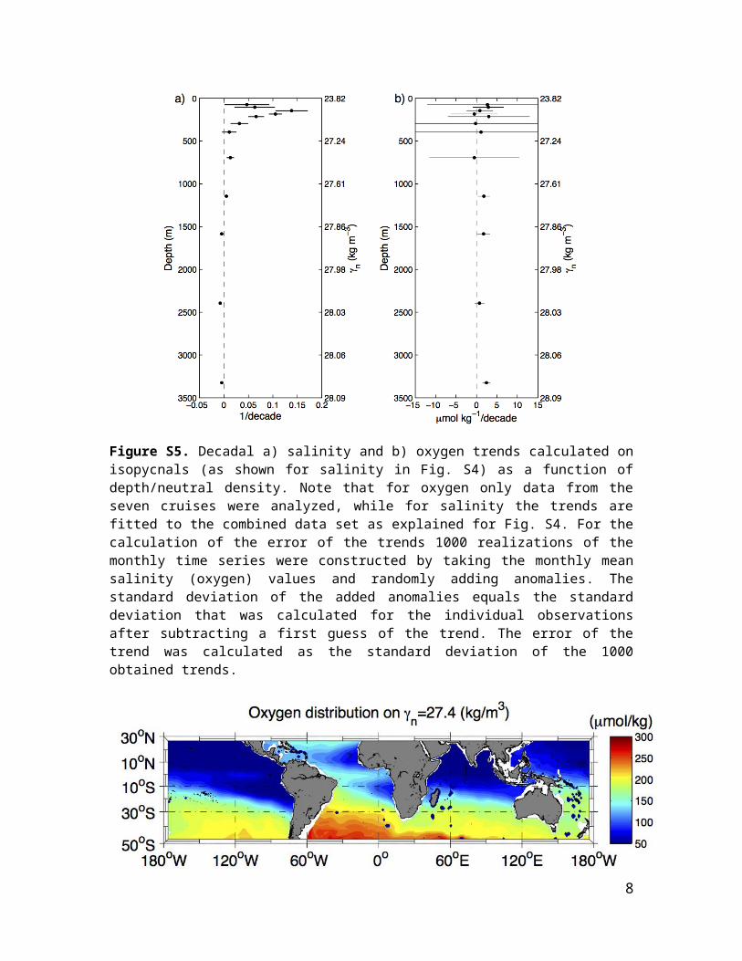
Figure S6. Mean oxygen distribution between latitudes 50°S and 30°N on neutral density surface γn=27.4 kgm-3 from the World Ocean Atlas 2013 showing higher oxygen levels in the South Atlantic compared to the South Indian Ocean.

References

Boebel, O., C. Schmid, and W. Zenk (1999), Kinematic elements of Antarctic Intermediate Water in the western South Atlantic, Deep Sea Research Part II: Topical Studies in Oceanography, 46(1–2), 355-392.

Dengler, M., F. A. Schott, C. Eden, P. Brandt, J. Fischer, and R. J. Zantopp (2004), Break-up of the Atlantic deep western boundary current into eddies at 8 degrees S, Nature, 432(7020), 1018-1020.

Durgadoo, J. V., B. R. Loveday, C. J. C. Reason, P. Penven, and A. Biastoch (2013), Agulhas Leakage Predominantly Responds to the Southern Hemisphere Westerlies, Journal of Physical Oceanography, 43(10), 2113-2131.

Large, W. G., and S. G. Yeager (2009), The global climatology of an interannually varying air–sea flux data set, Climate Dynamics, 33(2-3), 341-364.

Madec, G. (2008), NEMO ocean engine. Note du Pole de Modelisation d l'Institut Pierre-Simon Laplace 27, 215pp.

Schott, F. A., M. Dengler, R. Zantopp, L. Stramma, J. Fischer, and P. Brandt (2005), The shallow and deep western boundary circulation of the South Atlantic at 5 degrees-11 degrees S, Journal of Physical Oceanography, 35(11), 2031-2053.

Zhang, D., R. Msadek, M. J. McPhaden, and T. Delworth (2011), Multidecadal variability of the North Brazil Current and its connection to the Atlantic meridional overturning circulation, Journal of Geophysical Research: Oceans, 116(C4), C04012.

8