S1

Supporting Information for: The Effect of a Receding Saline

Lake (The Salton Sea) on Airborne Particulate Matter

Composition

Alexander L. Frie

1, Justin H. Dingle

2, Samantha C. Ying

1,2, and Roya Bahreini

1,2*

1Department of Environmental Sciences, University of California, Riverside, CA, 92521

2Environmental Toxicology Graduate Program, University of California, Riverside, CA 92521

*Correspondence to: Roya Bahreini (Roya.Bahreini@ucr.edu)

University of California, Riverside

900 University Ave.

Riverside, CA 92521

Tel: 951-827-4506

Fax: 951-827-4652

16 pages of Supporting Information

I. Page S2-S4, Supporting Text

II. Page S5-S8, Supporting Tables (Table S1-S4)

III. Page S9-S16, Supporting Figures (Figures S1-S9)

S2

I. Supporting Text

Description of Trace Metal Digest Procedure

To determine total metal and metalloid concentrations, samples were placed in a Teflon vial, and 2.5 ml of

concentrated HNO3 and 0.5 ml of concentrated HF were added. All acids were sourced from Fisher Chemical and

were trace metal grade or better. The closed vial was heated to 130-150 °C in an HEPA-filtered micro cleanroom,

under negative pressure for 15 hours. While maintaining clean conditions, the vial was then uncapped and heated to

130 °C until ~0.5 ml of liquid remained. To assure total digestion of trace metals, 0.6 ml of concentrated HNO3 and

1.8 ml of concentrated HCl were added to the vial for a second digestion. The closed vial was again heated on a hot

plate to 130-150 °C for 15 hours. The vial was then uncapped and heated at 130 °C until ~0.5 ml of liquid remained.

Finally, the solution was diluted with 2 ml of 5% HNO3. The exact solution volume was determined by weighing the

vial. The solution was transferred into an acid-cleaned 4 ml HDPE bottle and stored refrigerated until analysis.

An external geological standard (USGS G-2) was co-digested. For G-2, the relative method precision for all

metals was better than 15%, while recovery of certified species, Na, Al, K, Ca, Mn, Fe was >79%. Co and Ba were

the only certified species to display variation from the expected value by more than 21%. Lower than perfect mass

recovery and some mass lost is expected as digests are known to have incomplete mass closure.1 All aerosol data

were blank corrected using elemental concentrations from the digested field blanks.

PM10 mass concentrations of each element are calculated by summing the elemental concentration of all

digests (0.056 – 10 µm) for a specific aerosol sampling period. Filter digests resulting in values that were below the

method detection limit (BDL) for specific elements were included unadjusted in PM10 mass concentrations, as

replacement of a BDL value with “0” may skew the results. For a small subset of filter digests (6 of 129) where

contamination occurred during preparation, the median value of each element within the same size range was used

to replace the missing values when calculating PM10 mass concentrations.

Description of ED-XRF quantification

During ED-XRF analysis, United States Geologic Survey (USGS) standard reference material G-2 was also

analyzed as an external standard. G-2 measurements were precise: all metals having an RSD of less than 7%.

Variation from the expected value for certified species Na, Al, K, Ca, Fe was less than 30%. The only certified

species to display error greater than 30% were Ti and Mn.

Positive Matrix Factorization Case Description

Three separate PMF models were run using concentrations of each element within PM10, PM10-1, and PM1.

Missing data values (6 out of 129 digests), removed due to contamination during digestion, were replaced with the

S3

median value of the elemental mass concentration in that stage and given an uncertainty of 4 times this value. Below

detection limit data were included to avoid introducing biases.2 Internal PMF parameters, such as Qrobust, Qtrue, and

Qexpected were considered to assess performance of PMF. In general, Q is a measure of the fitness of the model; Qrobust

is calculated using only samples that fit the model well, while all samples are used in calculating Qtrue. Qexpected is

equal to the number of samples multiplied by the number of strong species. The normalized contribution of each

factor was constrained to above -0.2, and Qrobust was used per the settings of EPA PMF 5.0. Only results from the

PM10 model data are reported here, as the PM10, PM10-1 and PM1 results were observed to be qualitatively similar.

Ca, Na, As, Al Fe, Mn, V, Ba, Co, Se, Ti, K were classified as strong and Ni, Cd, Cr as weak species. Weak species

were identified by a S/N ratio of less than 2; S/N ratios were calculated by PMF 5.0. Fpeak was set to 0 and no

species were constrained to preset values. After running the model with 2-7 factors, a 4 factor solution was selected

because of a low Qtrue/Qexpected (5.8) (Fig. S9), small residuals for most species and samples, absence of rotational

ambiguity, and reasonable factor compositions. Within this solution, only Cd, Se, and Ba did not produce normally

distributed residuals. Furthermore, only weak species displayed R2 between distributions of observed vs. predicted

values of < 0.6, and most strong species displayed R2

values > 0.9, demonstrating the ability of this solution set to

reproduce the sample data well. The uncertainty was estimated using the displacement method (Paatero et al., 2014).

Bootstrapping was not used because of the small size of the sample set. High uncertainties were observed in the

contribution of certain species to each factor, but each factor contained at least one well-constrained species,

highlighting the dominant chemical characteristic of that factor. These high uncertainties stem, in part, from the high

and variable values of field blanks that are carried through the model. Rotational swaps, indicating uncertainty in the

identified components and their contributions, were not observed during displacement, and the largest change in Q

was -0.01%, evidencing the good fit of the solution set.

Temperature Description

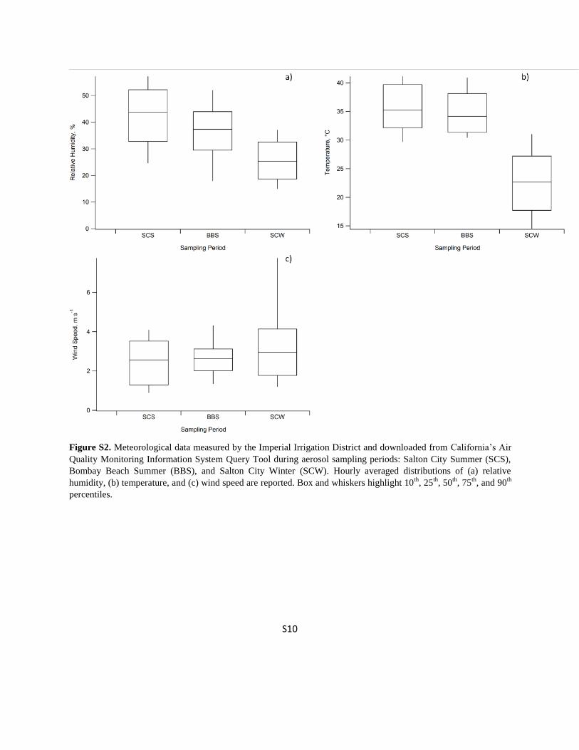
Ambient temperature (Fig. S2b) also displayed expected diurnal and seasonal variation, with the highest

temperatures observed during summer afternoons and lowest temperatures observed during winter mornings.

Average temperatures for BBS, SCS, and SCW at 06:00 LT (a proxy for the daily minimum temperature) were 31.8

°C, 31.6 °C, and 15.9 °C, respectively. Average temperatures for BBS, SCS, and SCW at 15:00 LT (a proxy for the

daily maximum temperature) were 41.5 °C, 41.3 °C, and 29.7 °C, respectively.

Wind Direction Analysis

For SCS and BBS daytime wind values were well confined: during the day at SCS, greater than 60%

occurrence of easterly winds (wind direction between 67.5° and 112.5°) was observed, while at BBS, wind direction

S4

was predominantly southeasterly/southerly (wind direction between 112.5° and 202.5°). SCS and BBS night periods

were more variable, with no octant having a probability greater than 35%. Despite this, BBS night wind directions

varied primarily between southwesterly and southeasterly, with very low probabilities of northerly winds. SCW

winds displayed the opposite diurnal variability trend, with night values having a dominant (90% probability)

westerly wind direction (between 202.5° and 292.5°). No wind direction octant displayed greater than 25%

probability during the day SCW periods.

References

1. Bettinelli, M., Beone, G. M., Spezia, S., and Baffi, C. Determination of heavy metals in soils and sediments

by microwave-assisted digestion and inductively coupled plasma optical emission spectrometry

analysis. Anal. Chim. Acta 2000, 424, 289–296; DOI 10.1016/S0003-2670(00)01123-5

2. Brown, S. G., Eberly, S., Paatero, P., and Norris, G. A. Methods for estimating uncertainty in PMF

solutions: examples with ambient air and water quality data and guidance on reporting PMF results. Sci.

Total Environ. 2015, 518–519, 626–635; DOI 10.1016/j.scitotenv.2015.01.022

S5

II. Supporting Tables

Element Average Desert, ppm Average Playa, ppm P Value, Playa vs Desert

Na 7.3e3 ± 3.3e3 7.2e4 ± 4.3e4 0.01

AL 4e4 ± 1.6e4 2.5e4 ± 8.2e3 0.04

K 1.4e4 ± 4.5e3 1.0e4 ± 2.5e3 0.04

Ca 2.9e4 ± 1.7e4 4.7e4 ± 1.4e4 0.02

Ti 3e4 ± 950 1.3e3 ± 460 0.00

V 55 ± 21 31 ± 14 0.02

Cr 31 ±13 18 ± 8 0.03

Mn 420 ± 180 210 ± 80 0.01

Fe 1.7e4 ± 8.8e3 1.0e4 ± 5.6e3 0.09

Co 6 ± 3 3 ± 2 0.03

Ni 13 ± 7 8 ± 4 0.12

Cu 15 ± 9 16 ± 18 0.15

Zn 49 ± 22 33 ± 15 0.15

As 7 ± 5 5 ± 3 0.27

Se 0.1 ± 0.1 0.5 ± 0.3 0.01

Cd 0.2 ± 0.1 0.2 ± 0.1 0.53

Ba 520 ± 200 250 ± 40 0.00

Pb 14 ± 6 7 ± 2 0.00

Table S1. Average elemental concentrations of playa and desert soils samples as measured via ICP-MS. P values

were calculated from a two tailed, heteroscedastic, student’s T test between the desert and playa samples. P value

less than or equal to 0.05 are highlighted.

S6

Element Average Desert, ppm Average Playa, ppm P Value, Playa vs Desert

Na 1.3e4 ± 5.e3 1.3e5 ± 8.3e4 0.00

Al 7.9e4 ± 1.2e4 5.2e4 ± 2.2e4 0.00

K 1.8e4 ± 2e3 1.2e4 ± 5e3 0.00

Ca 4.5e4 ± 9e3 5.9e4 ± 2.1e4 0.00

Ti 3.4e3 ± 1e3 1.8e3 ± 1e3 0.00

V 60 ± 20 50 ± 20 0.02

Cr 40 ± 10 20 ± 20 0.00

Mn 410 ± 100 250 ± 150 0.00

Fe 2.4e4 ± 6e3 1.5e4 ± 1.0e4 0.00

Co 50%<BDL 50%<BDL

NA

Zn 50 ± 20 40 ± 20 0.00

As 50%<BDL 10 ± 20 0.95

Se 50%<BDL 2 ± 2 0.00

Cd 50%<BDL 50%<BDL

NA

Pb 23 ± 5 15 ± 5 0.00

Table S2. Average elemental concentrations of playa and desert soils samples as measured via ED-XRF. P values

were calculated from a two tailed, heteroscedastic, student’s T test between the desert and playa samples. P value

less than or equal to 0.05 are highlighted.

S7

Element

Median,

PM10, ng m-1

Summer PM10,

ng m-1

Winter PM10,

ng m-1

Cal EPA Reference

Exposure Levels, ng m-1

P Value

Summer vs.Winter

Na 480 850 ± 690 370 ± 160 NA 0.02

Al 620 870 ± 580 1e3 ± 880 NA 0.69

K 280 380 ± 270 410 ± 280 NA 0.78

Ca 670 940 ± 1.0e3 1.4e3 ± 1.8e3 NA 0.43

Ti 44 63 ± 39 57 ± 46 NA 0.75

V 1.8 2.1 ± 1.3 1.9 ± 1.4 NA 0.64

Cr 9 12.4 ± 8.8 11.1 ± 9.8 200 (Cr VI) 0.74

Mn 9.2 13.2 ± 9.3 12.2 ± 8.7 90 0.78

Fe 390 600 ± 430 540 ± 410 NA 0.72

Co 0.3 0.4 ± 0.2 0.4 ± 0.3 NA 0.63

Ni 5.7 8 ± 4.7 8 ± 8.3 14 1.00

As 0.5 0.7 ± 0.7 0.4 ± 0.2 15 0.14

Se 0.9 2.2 ± 2.7 0.3 ± 0.4 20000 0.02

Cd 0.05 0.42 ± 1.01 0.06 ± 0.03 20 0.20

Ba 15 24 ± 19 16 ± 8 NA 0.19

Table S3. Median, seasonal average, and standard deviations of PM10 elemental concentrations, as measured via

ICP-MS. P values were calculated from a two tailed, heteroscedastic, student’s T test between the summer and

winter samples. P value less than or equal to 0.05 are highlighted.

S8

Element Median EF Average

Summer EF

Average Winter

EF

P Value,

Summer vs. Winter

Na 2.2 3 ± 0.79 1.7 ± 1.3 0.011

K 1.1 1.2 ± 0.33 1.3 ± 0.34 0.715

Ca 2.3 2.8 ± 2.7 2.5 ± 2.5 0.56

Ti 1.6 1.9 ± 0.66 1.5 ± 0.39 0.074

V 1.5 2.2 ± 1 1.7 ± 0.92 0.17

Cr 31 40 ± 33 30 ± 14 0.33

Mn 2.1 2.3 ± 0.36 2.1 ± 0.99 0.5

Fe 1.6 1.7 ± 0.39 1.5 ± 0.55 0.33

Co 3 4.2 ± 3.1 2.9 ± 0.92 0.17

Ni 42 48 ± 28 39 ± 20 0.39

As 27 21 ± 12 21 ± 10 0.034

Se 1200 2200 ± 1200 400 ± 460 0.0001

Cd 64 610 ± 1400 61 ± 31 0.15

Ba 2.9 3.7 ± 3.7 2.5 ± 1.2 0.24

Table S4: Median, seasonal average, and standard deviation of PM10 EFs. P values were calculated from a two

tailed, heteroscedastic, student’s T test between the summer and winter samples. P values less than or equal to 0.05

are highlighted.

S9

III. Supporting Figures

Figure S1. Map of soil and aerosol sampling sites. Labels represent the number of ED-XRF and ICP-

MS analyzed soil samples from each site, presented as ED-XRF;ICP-MS.

S10

Figure S2. Meteorological data measured by the Imperial Irrigation District and downloaded from California’s Air

Quality Monitoring Information System Query Tool during aerosol sampling periods: Salton City Summer (SCS),

Bombay Beach Summer (BBS), and Salton City Winter (SCW). Hourly averaged distributions of (a) relative

humidity, (b) temperature, and (c) wind speed are reported. Box and whiskers highlight 10th

, 25th

, 50th

, 75th

, and 90th

percentiles.

S11

Figure S3: Average diurnal relative humidity pattern for Salton City Winter (SCW, Blue), Bombay Beach Summer

(BBS, green), and Salton City Summer (SCS, red).

S12

Figure S4: Wind Roses for Salton City Summer (SCS) sampling period. The probability of wind being sourced

from a given direction is represented by the size of the colored portion and the colors represent wind speed

probabilities in m s-1

.

S13

Figure S5: Wind Roses for Salton City Winter (SCW) sampling period. The probability of wind being sourced from

a given direction is represented by the size of the colored portion and the colors represent wind speed probabilities

in m s-1

.

S14

Figure S6: Wind Roses for Bombay Beach Summer (BBS) sampling period. The probability of wind being sourced

from a given direction is represented by the size of the colored portion and the colors represent wind speed

probabilities in m s-1

.

S15

Figure S7. PM10 mass concentration as measured by the Imperial Irrigation District and downloaded from

California’s Air Quality Monitoring Information System Query Tool during aerosol sampling periods: Salton City

Summer (SCS), Bombay Beach Summer (BBS), and Salton City Winter (SCW). Box and whiskers highlight 10th

,

25th

, 50th

, 75th

, and 90th

percentiles.

Figure S8. Diurnal PM10 mass concentrations during Salton City Summer (SCS), Salton City Winter (SCW), and

Bombay Beach Summer (BBS) sampling as measured by TEOM ( Imperial Irrigation District, data available

through the AQMIS).

S16

Figure S9. Qtrue/Qexpected ratio of positive matrix factorization results with different factor number inputs. A 4 factor

model was selected as being the most accurate to describe the data because the change in Qtrue/Qexpected was

insignificant after addition of another factor.