support vector machines - cedar.buffalo.edusrihari/cse574/chap6/chap6.4-svms.pdf · alternative...

Machine Learning Srihari

Support Vector Machines

[email protected]


SVM Discussion Overview

1.  Importance of SVMs 2.  Overview of Mathematical Techniques

Employed 3.  Margin Geometry 4.  SVM Training Methodology 5.  Overlapping Distributions 6.  Dealing with Multiple Classes 7.  SVM and Computational Learning Theory 8.  Relevance Vector Machines


1. Importance of SVMs •  SVM is a discriminative method that

brings together: 1. computational learning theory 2. previously known methods in linear

discriminant functions 3. optimization theory

•  Widely used for solving problems in classification, regression and novelty detection


Alternative Names for SVM •  Also called Sparse kernel machines

•  Kernel methods predict based on linear combinations of a kernel function evaluated at the training points, e.g., Parzen Window

•  Sparse because not all pairs of training points need be used

•  Also called Maximum margin classifiers


2. Mathematical Techniques Used 1. Linearly separable case considered

since appropriate nonlinear mapping f to a high dimension two categories are always separable by a hyperplane

2. To handle non-linear separability •  Preprocessing data to represent in much higher-

dimensional space than original feature space •  Kernel trick reduces computational overhead

k(y

j,y

k) = y

jt ⋅y

k= φ(x

j)t ⋅φ(x

k)


Three support vectors are shown as solid dots

3. Support Vectors and Margin

•  Support vectors are those nearest patterns at distance b from hyperplane

•  SVM finds hyperplane with maximum distance

(margin distance b)

from nearest training patterns


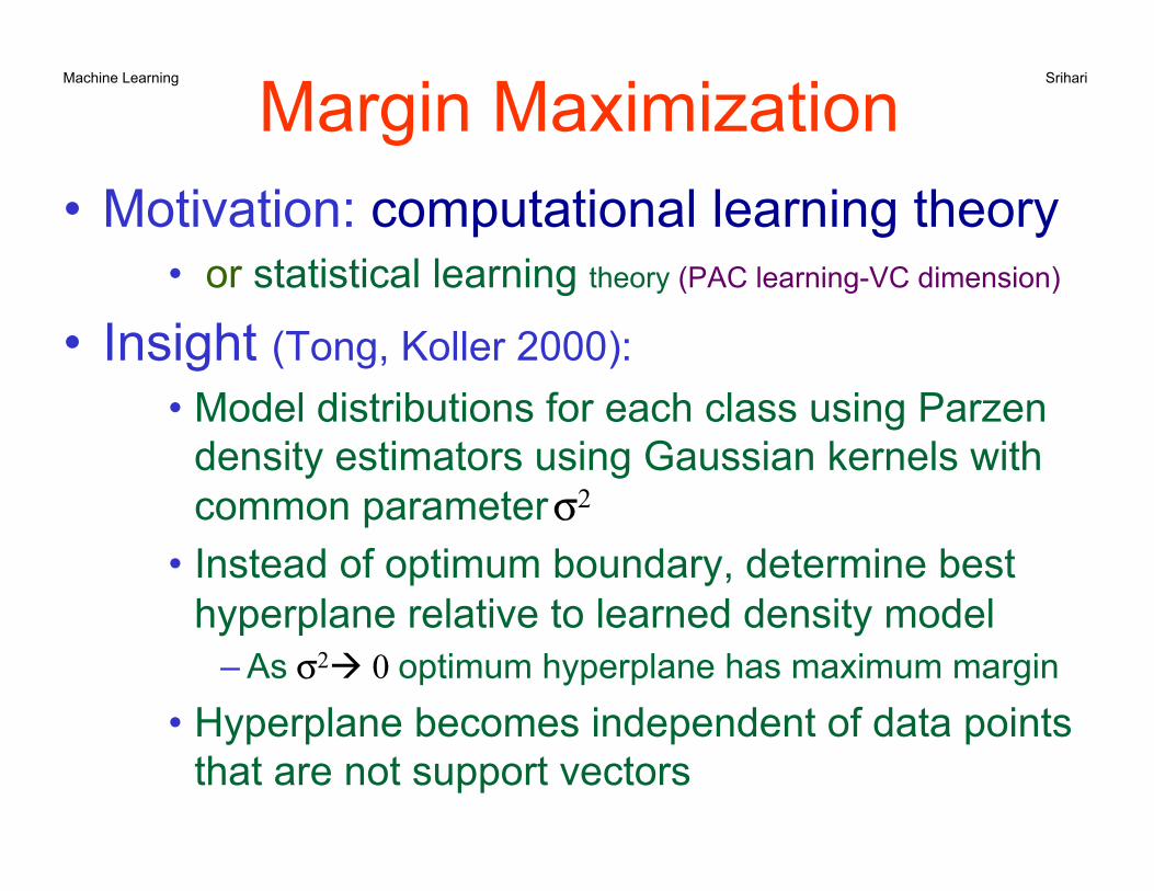
Margin Maximization •  Motivation: computational learning theory

•  or statistical learning theory (PAC learning-VC dimension)

•  Insight (Tong, Koller 2000): • Model distributions for each class using Parzen

density estimators using Gaussian kernels with common parameter σ2

•  Instead of optimum boundary, determine best hyperplane relative to learned density model

– As σ2à 0 optimum hyperplane has maximum margin

• Hyperplane becomes independent of data points that are not support vectors

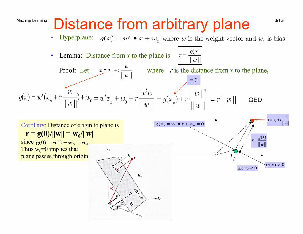
Machine Learning Srihari Distance from arbitrary plane •  Hyperplane:

•  Lemma:: Distance from x to the plane is Proof: Let where is the distance from x to the plane, then

|||| wwrxx p +=

||||)(

wxgr =

px0)( <yg

x = x

p+ r

w||w ||

g(x) = wt(x

p+ r

w||w ||

)+w0

= wtx

p+w

0+ r

wtw||w ||

= g(xp)+ r

||w ||2

||w || = r ||w ||

r r = g(x)

||w ||

0)( 0 =+•= wxwxg t

0)( >xg

Corollary: Distance of origin to plane is r = g(0)/||w|| = w0/||w|| since Thus w0=0 implies that plane passes through origin

000)0( wwwg t =+=

= 0

QED

g(x) = wt • x +w0 where w is the weight vector and w

0 is bias


Choosing a margin •  Augmented space: g(y) = aty by choosing a0= w0

and y0=1, i.e, plane passes through origin

•  For each of the patterns, let zk = +1 depending on whether pattern k is in class ω1 or ω2

•  Thus if g(y)=0 is a separating hyperplane then zk g(yk) > 0, k = 1,.., n

•  Since distance of a point y to hyperplane g(y)=0 is we could require that hyperplane be such that all points are at least distant b from it, i.e.,

zkg(y

k)

|| a ||≥ b

g(y)|| a ||

b

y g(y)= aty


g(y) = 1

SVM Margin geometry

Shortest line connecting Convex hulls, which has length = 2/||a||

Optimal hyperplane is orthogonal to..

y1 y2 g(y) = -1

g(y) = aty = 0 y2

y1


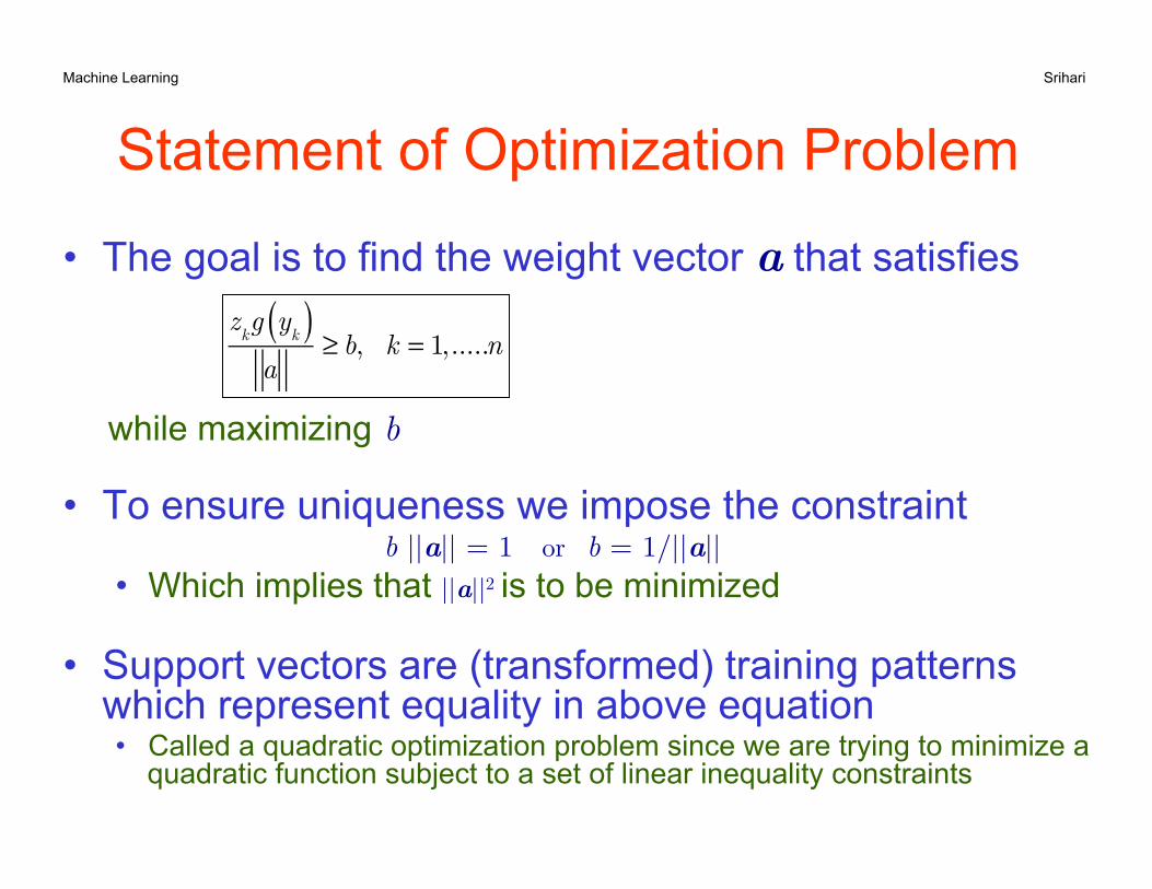
Statement of Optimization Problem

•  The goal is to find the weight vector a that satisfies

while maximizing b

•  To ensure uniqueness we impose the constraint b ||a|| = 1 or b = 1/||a||

•  Which implies that ||a||2 is to be minimized

•  Support vectors are (transformed) training patterns which represent equality in above equation •  Called a quadratic optimization problem since we are trying to minimize a

quadratic function subject to a set of linear inequality constraints

zkg y

k( )a

≥ b, k = 1,.....n


4. SVM Training Methodology

1.  Training is formulated as an optimization problem •  Dual problem is stated to reduce computational

complexity •  Kernel trick is used to reduce computation

2.  Determination of the model parameters corresponds to a convex optimization problem •  Solution is straightforward (local solution is a global

optimum) 3.  Makes use of Lagrange multipliers


Joseph-Louis Lagrange 1736-1813

•  French Mathematician •  Born in Turin, Italy •  Succeeded Euler at Berlin

academy •  Narrowly escaped execution

in French revolution due to Lovoisier who himself was guillotined

•  Made key contributions to calculus and dynamics


•  Can be cast as an unconstrained problem by introducing Lagrange undetermined multipliers with one multiplier for each constraint

•  The Lagrange function is

( ) [ ]∑=

−−=n

kk

tkk yaaaL

1

2 1z21, αα

SVM Training: Optimization Problem

nkyzsubject

optimize

kt

k ,.....1 ,1asconstraint to

||a||21min arg 2

ba,

=≥

α k


•  The Lagrange function is •  We seek to minimize L ( )

• with respect to the weight vector a and • maximize it w.r.t . the undetermined

multipliers •  Last term represents the goal of classifying the points correctly •  Karush-Kuhn-Tucker construction shows that this can be recast

as a maximization problem which is computationally better

( ) [ ]∑=

−−=n

kk

tkk yaaaL

1

2 1z21, αα

Optimization of Lagrange function

0≥α k


•  Problem is reformulated as one of maximizing •  Subject to the constraints given the training data

•  where the kernel function is defined by

( ) ∑∑∑= ==

−=n

kkjjkjk

n

j

n

kk yykL

1 11),(zz

21 αααα

Dual Optimization Problem

n1,.....,k ,0 0z1

=≥=∑=

kk

n

kk αα

)()(),( kt

jktjkj xxyyyyk φφ ⋅=⋅=


•  Implementation: •  Solved using quadratic programming •  Alternatively, since it only needs inner

products of training data •  It can be implemented using kernel functions •  which is a crucial property for generalizing to

non-linear case

•  The solution is given by

Solution of Dual Problem

kkk

k z ya ∑= α


Quadratic term

Summary of SVM Optimization Problems DifferentNotation here!


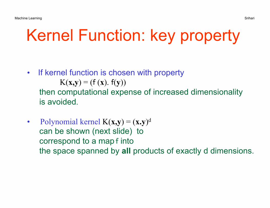
Kernel Function: key property

•  If kernel function is chosen with property K(x,y) = (f (x). f(y))

then computational expense of increased dimensionality is avoided.

•  Polynomial kernel K(x,y) = (x.y)d

can be shown (next slide) to correspond to a map f into the space spanned by all products of exactly d dimensions.


A Polynomial Kernel Function

•  Inner product needs computing six feature values and 3 x 3 = 9 multiplications

•  Kernel function K(x,y) has 2 mults and a squaring

( )

( ) ( )

( )( )( ))y()x()y,x(or

)(,,)y.x()y,x(

is valuesame thecompute ofunction t kernel Polynomial)(,2,,2,)y()x(

isproduct inner Then ,2,)x(

:is mapping space feature Thetor input vec theis ),( xSuppose

22211

2

21212

22211

2221

21

2221

21

2221

21

21

ϕϕ

ϕϕ

ϕ

=+===

+==

=

=

KyxyxyyxxK

yxyxyyyyxxxx

xxxx

xx

t

t

t

)()( yx ϕϕ

same


Another Polynomial (quadratic) kernel function

•  K(x,y) = (x.y + 1)2

•  This one maps d = 2, p = 2 into a six- dimensional space

•  Contains all the powers of x

•  Inner product needs 36 multiplications

•  Kernel function needs 4 multiplications

( ),1xx2,x2,x2,x,x)(

where)()(),(

212122

21=

=

x

yxyxK

ϕ

ϕϕ


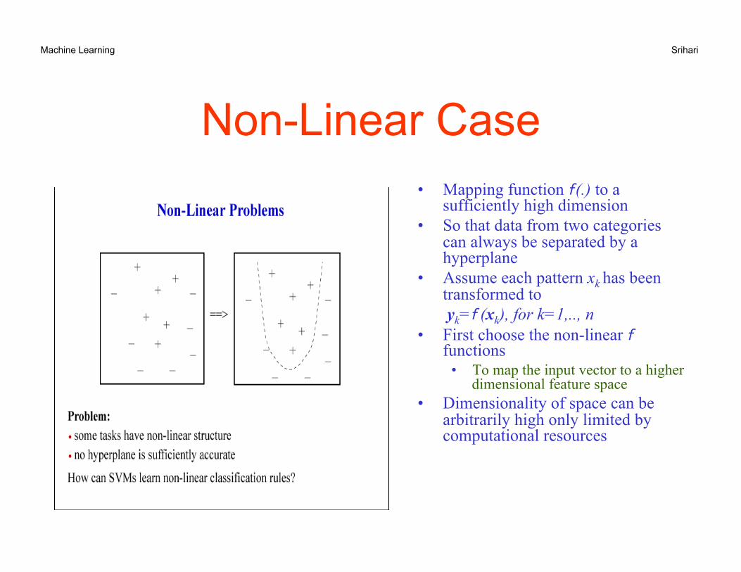
Non-Linear Case •  Mapping function f (.) to a

sufficiently high dimension •  So that data from two categories

can always be separated by a hyperplane

•  Assume each pattern xk has been transformed to yk=f (xk), for k=1,.., n

•  First choose the non-linear f functions

•  To map the input vector to a higher dimensional feature space

•  Dimensionality of space can be arbitrarily high only limited by computational resources


Mapping into Higher Dimensional Feature Space

•  Mapping each input point x by map

Points on 1-d line are mapped onto curve in 3-d.

•  Linear separation in 3-d space is possible. Linear discriminant function in 3-d is in the form

⎟⎟⎟

⎠

⎞

⎜⎜⎜

⎝

⎛=Φ=

2

1)(

xxxy

332211)( yayayaxg ++=


Pattern Transformation using Kernels

•  Problem with high-dimensional mapping •  Very many parameters •  Polynomial of degree p over d variables leads to O(dp) variables in

feature space •  Example: if d = 50 and p =2 we need a feature space of size

2500 •  Solution:

•  Dual Optimization problem needs only inner products

•  Each pattern xk transformed into pattern ykwhere

•  Dimensionality of mapped space can be arbitrarily high

)(xy kkΦ=


Example of SVM results •  Two classes in two

dimensions •  Synthetic Data •  Shows contours of constant

g (x) •  Obtained from SVM with

Gaussian kernel function •  Decision boundary is shown •  Margin boundaries are

shown •  Support vectors are shown •  Shows sparsity of SVM


SVM for the XOR problem •  XOR: binary valued features x1, x2 •  not solved by linear discriminant •  function f maps input x = [x1, x2] into six-

dimensional feature space y = [1, /2x1, /2x2, /2x1x2 , x1

2 , x22]

Hyperbolas Corresponding to x1 x2 = +1

Hyperplanes Corresponding to /2x1 x2 = +1

input space feature sub-space


∑∑∑===

−4

1

4

1

4

1zz

21

jk

tjkjjk

kkk yyααα

SVM for XOR: maximization problem •  We seek to maximize

•  Subject to the constraints

•  From problem symmetry, at the solution

,4 ,3 ,2 ,1 0

04321

=≤

=−+−

kkα

αααα

4231 and, αααα ==


SVM for XOR: maximization problem

•  Can use iterative gradient descent •  Or use analytical techniques for small problem •  The solution is

a* = (1/8,1/8,1/8,1/8) •  Last term of Optimizn Problem implies that all four points are support vectors (unusual and due to symmetric nature of XOR) •  The final discriminant function is g(x1,x2) = x1. x2 •  Decision hyperplane is defined by g(x1,x2) = 0 _ •  Margin is given by b=1/||a|| = \/2

Hyperbolas Corresponding to x1 x2 = +1

Hyperplanes Corresponding to _ \/2x1 x2 = +1


5. Overlapping Class Distributions

•  We assumed training data are linearly separable in the mapped space y • Resulting SVM gives exact separation in

input space x although decision boundary will be nonlinear

•  In practice class-conditionals overlap •  Exact separation leads to poor generalization •  Therefore need to allow SVM to misclassify

some training points


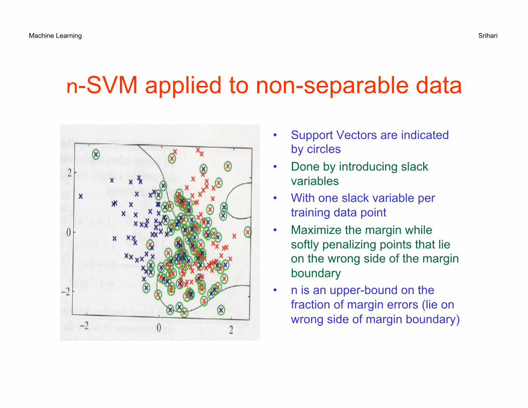
n-SVM applied to non-separable data

•  Support Vectors are indicated by circles

•  Done by introducing slack variables

•  With one slack variable per training data point

•  Maximize the margin while softly penalizing points that lie on the wrong side of the margin boundary

•  n is an upper-bound on the fraction of margin errors (lie on wrong side of margin boundary)


6. Multiclass SVMs (one-versus rest) •  SVM is a two-class classifier •  Several suggested methods for combining

multiple two-class classfiers •  Most used approach: one versus rest

•  Also recommended by Vapnik •  using data from class Ck as the positive examples

and data from the remaining k-1 classes as negative examples

•  Disadvantages •  Input assigned to multiple classes simultaneously •  Training sets are imbalanced (90% are one class and

10% are another)– symmetry of original problem is lost


Multiclass SVMs (one-versus one)

•  Train k(k-1)/2 different 2-class SVMs on all possible pairs of classes

•  Classify test points according to which class has highest number of votes

•  Again leads to ambiguities in classification •  For large k requires significantly more

training time than one-versus rest •  Also more computation time for evaluation

• Can be alleviated by organizing into a directed acyclic graph (DAGSVM)


7. SVM and Computational Learning Theory

•  SVM motivated using COLT • Called PAC learning framework

•  Goal of PAC framework is to understand how large a data sets needs to be in order to give good generalizations •  Key quantity in PAC learning is VC dimension

which provides a measure of complexity of a space of functions

•  Maximizing margin is main conclusion


All dichotomies of 3 points in 2 dimensions are linearly separable


VC Dimension of Hyperplanes in R2

Hyperplanes in Rd è VC Dimension = d+1

VC dimension provides the complexity of a class of decision functions


Fraction of Dichotomies that are linearly separable

Fraction of dichotomies of n points in d dimensions that are linearly separable

⎪⎩

⎪⎨⎧

+>⎟⎟⎠

⎞⎜⎜⎝

⎛ −=

+≤

=∑

1 1

01

12),(

dnd

i

n dnin

dnf

At n = 2(d+1), called the capacityof the hyperplane nearly one half of the dichotomies are still linearly separable

Hyperplane is not over-determineduntil number of samples is severaltimes the dimensionality

Capacity of a hyperplane

Fraction of dichotomies of n points in d dimensions that are linear

0.5 f(n,d

)

n/(d+1)

When no of points is same as dimensionality all dichotomies are linearly separable


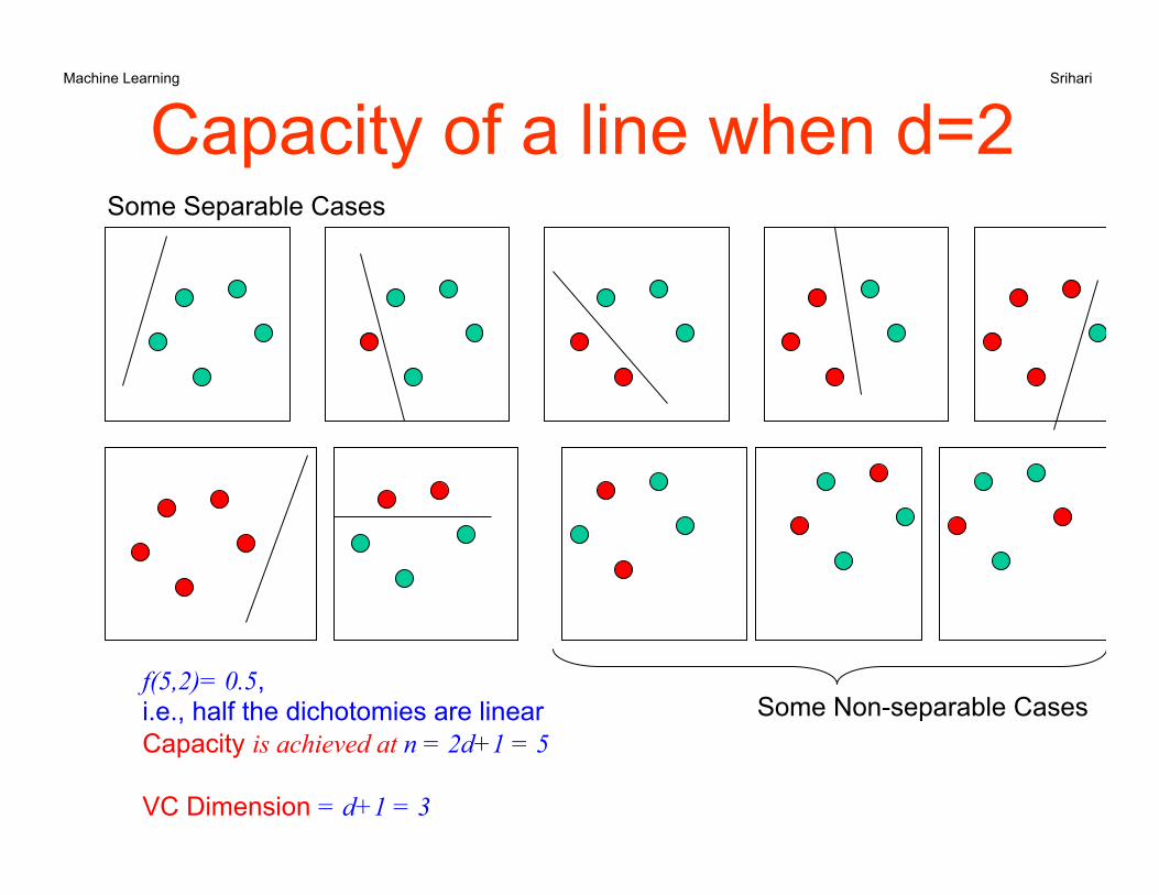
Capacity of a line when d=2

Some Non-separable Cases

Some Separable Cases

f(5,2)= 0.5, i.e., half the dichotomies are linear Capacity is achieved at n = 2d+1 = 5 VC Dimension = d+1 = 3


Possible method of training SVM

•  Based on modification of Perceptron training rule given below

Instead of all misclassified samples, use worst classified samples


Support vector samples •  Support vectors are

•  training samples that define the optimal separating hyperplane

•  They are the most difficult to classify •  Patterns most informative for the

classification task •  Worst classified pattern at any stage

is the one on the wrong side of the decision boundary farthest from the boundary

•  At the end of the training period such a pattern will be one of the support vectors

•  Finding worst case pattern is computationally expensive

•  For each update, need to search through entire training set to find worst classified sample

•  Only used for small problems

•  More commonly used method is different


•  If there are n training patterns •  Expected value of the generalization

error rate is bounded according to

Expected value of error < expected no of support vectors/n

•  Where expectation is over all training sets of size n (drawn from distributions describing the categories)

•  This also means that error rate on the support vectors will be n times the error rate on the total sample

[ ] [ ]n

errorP nn

VectorsSupport of .No)( εε ≤

Generalization Error of SVM

•  Leave one out bound

•  If we have n points in the training set

•  Train SVM on n-1 of them •  Test on single remaining point •  If the point is a support vector

then there will be an error •  If we find a transformation f

•  that well separates the data, then

–  expected number of support vectors is small

–  expected error rate is small


8. Relevance Vector Machines

•  Addresses several limitations of SVMs •  SVM does not provide a posteriori probabilities

•  Relevance Vector Machines provide such output

•  Extension of SVM to multiclasses is problematic •  Complexity parameter C or n that must be found

using a hold-out method •  Linear combinations of kernel functions centered

on training data points that must be positive definite

support vector machines - cedar.buffalo.edusrihari/cse574/chap6/chap6.4-svms.pdf · alternative...

Documents